Explaining and Improving Model Behavior with $k$ Nearest Neighbor Representations

Abstract

Interpretability techniques in NLP have mainly focused on understanding individual predictions using attention visualization or gradient-based saliency maps over tokens. We propose using $k$ nearest neighbor ($k$NN) representations to identify training examples responsible for a model’s predictions and obtain a corpus-level understanding of the model’s behavior. Apart from interpretability, we show that $k$NN representations are effective at uncovering learned spurious associations, identifying mislabeled examples, and improving the fine-tuned model’s performance. We focus on Natural Language Inference (NLI) as a case study and experiment with multiple datasets. Our method deploys backoff to $k$NN for BERT and RoBERTa on examples with low model confidence without any update to the model parameters. Our results indicate that the $k$NN approach makes the finetuned model more robust to adversarial inputs.

Introduction

Deep learning models are notoriously opaque, leading to a tremendous amount of research on the inscrutability of these so-called black-boxes. Prior interpretability techniques for NLP models have focused on explaining individual predictions by using gradient-based saliency maps over the input text (Lei, Barzilay, and Jaakkola 2016; Ribeiro, Singh, and Guestrin 2018; Bastings, Aziz, and Titov 2019) or interpreting attention (Brunner et al. 2020; Pruthi et al. 2020). These methods are limited to understanding model behavior for example-specific predictions.

In this work, we deploy $k$ Nearest Neighbors ($k$NN) over a model’s hidden representations to identify training examples closest to a given evaluation example. By examining the retrieved representations in the context of the evaluation example, we obtain a dataset-level understanding of the model behavior. Taking the NLI problem as an example (Figure 1), we identify the confidence interval where $k$NN performs better than the model itself on a held-out validation set. During inference, based on the model’s confidence score we either go forward with the model’s prediction or backoff to its $k$NN prediction. Our implementation of $k$NN can be used with any underlying neural classification models and it brings three main advantages:

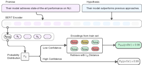
Figure 1: Overview of our proposed approach on using $k$NN as backoff to improve fine-tuned classification models.

• Explaining model behavior. Our $k$NN approach is able to explain a model’s prediction by tracing it back to the training examples responsible for that prediction. Although it sounds similar with influence functions (Koh and Liang 2017), our approach is much simpler because it does not access the model parameters and is approximately $300\times$ faster on small datasets ($<2K$ examples) and the gap increases on bigger datasets.

• Uncovering spurious associations. We observe that our $k$NN model can learn more fine-grained decision boundaries due to its added non-linearity, which can make it more robust to certain kinds of spurious correlations in the training data. We leverage this robustness for studying where models go wrong, and demonstrate how retrieving the nearest neighbors of a model’s misclassified examples can reveal artifacts and spurious correlations. From our analysis, we also observed that $k$NN of misclassified test examples can often retrieve mislabeled examples, which makes this approach applicable to fixing mislabeled ground truth examples in training sets.

• Improving model predictions. Along with providing a lens into understanding model behavior, we propose an approach that interpolates model predictions with $k$NN for classification by identifying a more robust boundary between classes. We are the first to demonstrate this using $k$NN for both interpretability and for improving model performance.

In summary, we propose a $k$NN framework that uses hidden representations of fine-tuned models to explain their underlying behaviors, unveil learned spurious correlations and further improve the model predictions. Through $k$NN we shed light on some of the existing problems in NLI datasets and deep learning models, and suggest some evaluation prescriptions based on our findings. To our knowledge, this is the first work that uses $k$NN in the representation space of deep neural models for both understanding and improving model behavior.

Related work

Our work is related to three main areas of research: approaches for interpretability in NLP, retrieval-based methods, and work on dataset artifacts and spurious associations.

Interpretability methods in NLP.

Our approach of using $k$NN to retrieve nearest training examples as an interpretability technique is model-agnostic. LIME (Ribeiro, Singh, and Guestrin 2016) is another model-agnostic method that interprets models by perturbing inputs and fitting a classifier in the locality of the model’s predictions for those perturbations. It has been extended to identifying artifacts and biases in information retrieval (Singh and Anand 2018). Alvarez-Melis and Jaakkola (2017) probe the causal structure in sequence generation tasks by perturbing the input and studying its effect on the output. The explanation consists of tokens that are causally related in each input-output pair.

Our method is closely related to the work on influence functions (Koh and Liang 2017) which has been recently extended by Han, Wallace, and Tsvetkov (2020) to neural text classifiers. Influence function are accurate for convex only when the model is strictly convex and so the authors approximation to the influence functions on BERT (Devlin et al. 2018). The authors evaluate the effectiveness by comparing them with gradient-based saliency methods for interpretability. Our approach uses FAISS (Johnson, Douze, and Jégou 2019) to create a cache once and so is computationally efficient and scalable to very large datasets that deep learning models rely on.

Interpreting attention as a form of explanation for neural NLP models has been a topic of debate (Jain and Wallace 2019; Serrano and Smith 2019; Wiegreffe and Pinter 2019). Zhong, Shao, and McKeown (2019) train attention to directly attend to human rationales and obtain more faithful explanations. Recent work has manipulated attention in Transformer (Vaswani et al. 2017) models in an attempt to make it more interpretable (Pruthi et al. 2020; Brunner et al. 2020). Gradient-based saliency maps are faithful by construction and hence have been applied in various forms to neural models for interpretability (Lei, Barzilay, and Jaakkola 2016; Ribeiro, Singh, and Guestrin 2018; Chang et al. 2019; Bastings, Aziz, and Titov 2019).

Retrieval-based approaches.

Many language generation methods use retrieval-based techniques at test time. Weston, Dinan, and Miller (2018) improve a dialogue response generation model by retrieving and refining similar instances from the training set. Gu et al. (2018) propose a Neural Machine Translation approach that fuses information from the given source sentence and a set of retrieved training sentence pairs. The neural cache (Grave, Joulin, and Usunier 2017) and related unbounded neural cache (Grave, Cisse, and Joulin 2017) retrieve similar instances from the sequence history to better adapt language models to the context. The recently introduced $k$NN language model ($k$NN-LM) extends on existing pre-trained language models by interpolating the next word distribution with a $k$NN model (Khandelwal et al. 2020). The combination is a meta-learner that can be effectively tuned for memorizing and retrieving rare long-tail patterns. Our work adapts the $k$NN-LM to text classification by using the input example as context, in a similar way to how deep-$k$NN (Papernot and McDaniel 2018) applies $k$NN over neural network representations to the classification of images. We show that our approach outperforms fine-tuned models like BERT and RoBERTa (Liu et al. 2019) and is particularly good as a backoff for a model’s less confident examples.

In addition to kNN-LM style approaches that interpolate the next word distribution, there has also been work leveraging the kNN training examples of a test instance to fine-tune a pretrained model (Zhao et al. 2020), which avoids the need to create new model architecture and train from scratch. For example, (Li, Zhang, and Zong 2018) search for similar sentence pairs from the training corpus for each testing sentence, which are then used to finetune the model.

Dataset artifacts and spurious associations.

Neural models have been very successful on various NLP tasks but a deeper understanding of these models has revealed that these models tend to exploit dataset artifacts. In Natural Language Inference (NLI), the hypothesis-only baseline is known to significantly outperform the majority baseline on both the SNLI (Bowman et al. 2015) and MNLI (Williams, Nangia, and Bowman 2018) datasets (Gururangan et al. 2018; Poliak et al. 2018). Pre-trained models like BERT rely on spurious syntactic heuristics such as lexical overlap for NLI (McCoy, Pavlick, and Linzen 2019). Various forms of data augmentations and evaluations for robustness have been proposed to overcome these limitations.  Kaushik, Hovy, and Lipton (2020) use counterfactual augmentation for SNLI to alleviate the bias from annotation artifacts. Their findings show that training on counterfactuals makes models more robust. We use $k$NN to study the shift in representations before and after the augmentation in terms of spurious signals. Our findings suggest that although counterfactual augmentation does help with reducing the effects of prominent artifacts like lexical overlap, it also inadvertently introduces new artifacts not present in the original dataset.

Method

Figure 1 shows an overview of our proposed approach that leverages $k$NN to improve an underlying classification model. Our implementation of $k$NN relies on caching the model’s output hidden representation of every training sequence. During inference, we query the cache to retrieve the nearest neighbors for a given example and make a prediction based on the weighted distance for each class.

Learning hidden representations

Our approach to $k$NN over hidden representations closely relates to $k$NN-LM implemented by Khandelwal et al. (2020) but has an extra normalization step over hidden states and a different method for interpolating $k$NN and neural networks for classification.

Our implementation assumes that we have a training set of sequences where each sequence $x^{i}$ is paired with a target label $y^{i}$. Our algorithm maps each $x^{i}$ to a hidden representation vector $h^{i}\in\mathbb{R}^{d}$, where $d$ is the hidden state dimension, using function $f_{\theta}$ defined by a neural network with parameters $\theta$:

$$h^{i}=f_{\theta}(x^{i})$$

In this work, these hidden states are obtained from BERT or RoBERTa systems. They are crucial in determining the performance of our method. We found that the [CLS] representation of the last layer of BERT or RoBERTa performs the best. As prescribed in (Reimers and Gurevych 2019), we also experimented with other pooling strategies like mean and max pooling of hidden representations across all time steps but the improvements were smaller compared to the [CLS] representation. We also evaluated using the best layers identified for capturing input semantics in generation for various transformer models (Zhang et al. 2019). However, we found that the last layer worked best and so all our models use the [CLS] representation of the last layer.

Those hidden representations can be collected and cached with one forward pass through the training set. For scaling to larger data sets, FAISS implements data structures for storing the cache that allows for faster $k$NN lookup and reduces memory usage. We then apply dataset-wise batch normalization (Ioffe and Szegedy 2015) to the hidden state vectors with means $\mu\in\mathbb{R}^{d}$ and standard deviations $\sigma\in\mathbb{R}^{d}$ over the hidden states, and obtain normalized hidden states using

$$\tilde{h}^{i}=\frac{h^{i}-\mu}{\sigma+\epsilon},$$

with a small $\epsilon$ for numerical stability. We map each test sequence $x^{\prime}$ to a fixed-size hidden state $\tilde{h}^{\prime}$ with

$$\tilde{h}^{\prime}=\frac{f_{\theta}(x^{\prime})-\mu}{\sigma+\epsilon}.$$

When the training set is large, it is possible to estimate means and variances from a subset of training sequences.

$K$ nearest neighbors over hidden representations

For $k$ nearest neighbors, we first locate the set of indices $K$ for $i$ which leads to the smallest $L_{2}$ distances given by $d^{i}=||\tilde{h}^{\prime}-\tilde{h}^{i}||^{2}$. Next, we compute the weighted $k$NN probability scores $w_{knn}(x^{i},x^{\prime})$ with a softmax over negative distances given by

$$w_{knn}(x^{i},x^{\prime})=\begin{cases}\frac{\exp(-d^{i}/T)}{\sum_{j\in K}\exp(-d^{j}/T)},&\text{if }i\in K\\ 0,&\text{otherwise.}\end{cases}$$

where $T$ is a temperature hyper-parameter that controls the sharpness of the softmax. The probability distribution over labels for the test sequence, $p_{knn}(y|x^{\prime})$ is then given by

$$p_{knn}(y|x^{\prime})=\sum_{j\in K}w_{knn}(x^{j},x^{\prime})\times e_{(y^{j})}$$

where $e_{(y^{j})}$ is a one-hot encoding of $y^{j}$ equal to one at the index of $y^{j}$ and zero at the index of all other labels. $p_{knn}(y|x^{\prime})$ can be used directly as a classifier or interpolated with the base neural network probability distribution $p_{\theta}(y|x^{\prime})$ in various ways.

In this work, we backoff to a $k$NN classifier depending on pre-defined criteria, such as when the model is less-confident in its predictions or if the model is known to perform poorly on certain types of inputs. Given some threshold hyper-parameter $\tau$, our classifier prediction is given by

$$y=\begin{cases}\operatorname*{arg\,max}p_{\theta}(y|x^{\prime}),&\text{if }\max p_{\theta}(y|x^{\prime})>\tau\\ \operatorname*{arg\,max}p_{knn}(y|x^{\prime}),&\text{otherwise}\end{cases}$$

The hyper-parameters $\tau$ and $T$ are determined based on each model and the validation set. We tune the value of $k$ on the validation set of each dataset, and use the same value for all models trained on that dataset.

Experiments

Datasets

We demonstrate the effectiveness of $k$NN on the natural language inference (NLI) task as a case study. The input to the NLI model is a pair of sentences – the premise and the hypothesis, and the task is to predict the relationship between the two sentences. The possible labels are ‘entailment’,‘contradiction’, or ‘neutral’. This problem requires complex semantic reasoning of underlying models (Dagan, Glickman, and Magnini 2005).

Apart from the vanilla version of the task, we also compare to augmented and adversarial versions of the original datasets to gain a deeper understanding of how the model behavior changes.

• SNLI: The Stanford Natural Language Inference (SNLI) (Bowman et al. 2015) dataset is a widely used corpus for the NLI task. Recently,  Kaushik, Hovy, and Lipton (2020) released a counterfactually augmented version of the SNLI. The new corpus consists of a very small sample of the original dataset ($0.3\%$) called the original split. The original split is augmented with counterfactuals by asking crowdworkers to make minimum changes in the original example that would flip the label. This leads to three more splits – the revised premise wherein only the premise is augmented, the revised hypothesis wherein only the hypothesis is augmented or the combined that consists of both premise and hypothesis augmentations along with the original sentence pairs.

We use the original and combined splits (refered to as augmented split) in our experiments that have training data sizes of 1666 and 8330 respectively. For validation and testing on the original split, we use the SNLI validation and test sets from Bowman et al. (2015) with sizes 9842 and 9824, respectively. For the combined split, we validate and test on the combined validation and test sets with sizes 1000 and 2000, respectively.

• ANLI: To overcome the problem of models exploiting spurious statistical patterns in NLI datasets, Nie et al. (2020) released the Adversarial NLI (ANLI) dataset.  ANLI is a large-scale NLI dataset collected via an iterative, adversarial human-and-model-in-the-loop procedure. In each round, a best-performing model from the previous round is present, then human annotators are asked to write “hard” examples the model misclassified. They always choose multi-sentence paragraphs as premises and write single sentences as hypotheses. Then a part of those “hard” examples join the training set so as to learn a stronger model for the next round. The remaining part of “hard” examples act as dev/test set correspondingly. In total, three rounds were accomplished for ANLI construction. We put the data from the three rounds together as an overall dataset, which results in train/validation/test split sizes of $162,865$/$3200$/$3200$ input pairs.

P: A man wearing a white shirt and an orange shirt jumped into the air.

H: A man’s feet are not touching the ground.   GT: [entailment]

P: Two boxers are fighting and the one in the purple short is attempting to block a punch. H: Both boxers wore black pants.   GT: [contradiction]

P: A woman wearing a purple dress and black boots walks through a crowd drinking from a glass bottle. H: The woman is drinking from a plastic bottle.   GT: [contradiction]

P: The woman in purple shorts and a brown vest has a black dog to the right of her and a dog behind her. H: A woman is walking three dogs.   GT: [contradiction]

P: A young lady wearing purple and black is running past an orange cone. H: The young lady is walking calmly.   GT: [contradiction]

P: A man and woman stand in front of a large red modern statue. H: The man and woman are not sitting.   GT: [entailment]

P: Three guys sitting on rocks looking at the scenery. H: The people are not standing.   GT: [entailment]

P: Two boys are playing ball in an alley. H: The boys are not dancing.   GT: [entailment]

P: A girl is blowing at a dandelion. H: The girl isn’t swimming in a pool.   GT: [entailment]

Table 1: The first block shows an example from the original dev set that BERT predicts incorrectly as contradiction when trained on the SNLI original split but predicts correctly as entailment when trained with the counterfactual augmentations. Only showing top $k$ = 4 examples. Bold text indicates uncovered likely spurious association between mention of colors and contradiction.

• HANS: Heuristic Analysis for NLI Systems (HANS) (McCoy, Pavlick, and Linzen 2019) is a controlled evaluation dataset aiming to probe if a model has learned the following three kinds of spurious heuristic signals: lexical overlap, subsequence, and constituent. This dataset intentionally includes examples where relying on these heuristics fail by generating from $10$ predefined templates. This dataset is challenging because state-of-the-art models like BERT (Devlin et al. 2018) perform very poorly on it. There are in total $30,000$ examples – $10,000$ for each heuristic.

We use this dataset only for validating and testing our models that are trained on the ANLI dataset. The HANS dataset has only two classes, ‘entail’ and ‘not-entail’ while ANLI has 3 classes so we collapse the ‘neutral’ and ‘contradiction’ predictions into ‘not-entail’. We randomly split 30K examples into 10K for validation and 20K for testing while maintaining the balance across the different heuristics in both the splits.

System setup

We focus on experimenting with two transformer models – the BERT and RoBERTa. For both models we only use their base versions with 110M and 125M parameters. More details about the hyper-parameters used for each of these models are mentioned in Appendix A.

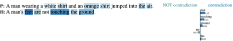
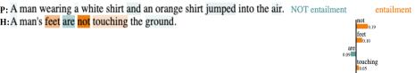
Figure 2: LIME saliency map highlighting the top feature words in the BERT model’s prediction. The top figure shows that the model uses the occurrence of colors as important features, verifying the spurious pattern of associating colors with the contradiction class that is uncovered by kNN in Table 1 (middle block). The bottom figure shows the contrast that after augmentation the model does not use color features and so is able to make the right prediction (entailment).

Results

We use $k$NN as a lens into interpreting and understanding model behavior based on its learned representations. Specifically, we explore the effectiveness of $k$NN on uncovering spurious associations and identifying mislabeled training examples. In the following sections, we describe these application of $k$NN using NLI as a case study.

• Explaining the model behavior using nearest training examples. The most similar training examples retrieved by $k$NN provide context for a given input in the representation space of the model, thereby providing an understanding for why the model made a certain prediction. We run experiments to test at the dataset level if the retrieved training examples are actually the ones that the model relies on to learn its decision boundary. We do this by removing a percentage of the training examples most frequently retrieved by $k$NN  (with $k=16$) on the training set, retrain the model from initialization, and re-evaluate the model. We repeat this procedure and average results over three random seeds. On the original SNLI split, we find that on average BERT’s performance drops by $4.6\%$ when the top $10\%$ of the $1666$ training examples are removed vs. $1.2\%$ when an equal amount of random examples are removed. The performance further drops by another $6\%$ when the percentage is increased to $30\%$ vs. $4\%$ for random. This experiment verifies that a model’s prediction for a specific testing example is highly correlated with its neighboring examples in training set. Tables 2 and  3 show top (based on distance) influential training examples for a dev example.

P: A young man dressed in black dress clothes lies down with his head resting in the lap of an older man in plain clothes.

H: One man is dressed up for a night out while the other is not.

GT: [neutral]

P: There is a performance with a man in a t-shirt and jeans with a woman in all black while an audience watches and laughs.

H: The man and woman are friends.   GT: [neutral]

P:A man in a black shirt plays the guitar surrounded by drinks.

H: The man is skilled at playing.   GT: [neutral]

P: An older guy is playing chess with a young boy.

H: Two generations play an ancient game.   GT: [entailment]

P: A young girl skiing along side an adult.

H: The young girl is the adult’s child.   GT: [neutral]

P: Many people in white smocks look at things under identical looking microscopes. H: Multiple humans are not looking under microscopes.   GT: [entailment]

P: A small girl dancing in a parade wearing bright red and gold clothes. H: The small girl is sitting at home, not celebrating.   GT: [contradiction]

P: A five-piece band, four of the men in red outfits and one of them in a leather jacket and jeans, perform on the sidewalk in front of a shop.

H: The five-piece band of women in red is not performing.   GT: [contradiction]

P: Three young girls chapping and texting on a cellphone. H: Three young girls are sitting together and not communicating.   GT: [contradiction]

Table 2: This table contrasts the results of $k$NN when training BERT on original SNLI vs. with counterfactual augmentations. $k$NN reveals artifacts in the SNLI augmented split that cause the BERT’s prediction on a dev example (first block) to go from neutral when trained on the SNLI original split (second block) to contradiction when trained with counterfactual augmentation (third block). Only showing top $k$ = 4 examples. Bold text indicates likely spurious correlation. Some examples have mislabeled GT but kNN is robust in identifying similar examples.

• Uncovering spurious associations. Spurious associations are caused by a model confounding the statistical co-occurrence of a pattern in the input and a class label with high mutual information between the two. For example, state-of-the-art models are known to associate high lexical overlap between the premise and the hypothesis with the label entailment (McCoy, Pavlick, and Linzen 2019). So models that rely on this association fail spectacularly when the subject and the object are switched. Counterfactual data augmentation alleviates this problem by reducing the co-occurrence of such artifacts and the associated class label.

$k$NN provides a tool for uncovering potential spurious associations. First, we examine the nearest neighbors of misclassified examples for possible spurious patterns. Next, we use feature-importance methods like LIME to verify the pattern by comparing it to the highest-weighted word features. Table 1 shows potential spurious association between mention of colors and contradiction label uncovered by $k$NN when BERT is trained on the original split. As shown, counterfactual augmentation helps in debiasing the model and BERT is then able to classify the same example correctly.

Surprisingly, through $k$NN we also find that counterfactual augmentation inadvertently introduces new artifacts that degrade model performance on certain data slices. Table 2 shows an example where BERT’s prediction goes from neutral to contradiction when trained on augmented data. The nearest neighbors reveal that BERT learns to correlate the occurrence of negation in the hypothesis with contradiction. LIME verifies that the most highly weighted feature is the occurrence of ‘not’ as shown in Figure 3. Quantitatively, we verify that the pattern ‘not’ occurs approximately $37\%$ and $60\%$ of times in the original and augmented training splits of SNLI respectively. The accuracy of BERT on identifying entailment examples that contain negation drops by $10\%$ when trained with augmented data versus without. Figure 3 shows the saliency map of words that were highly-weighted in BERT’s prediction using LIME. As expected, the model trained on augmented data learns to spuriously associate the occurrence of ‘not’ with the contradiction class.

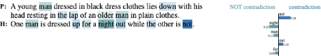
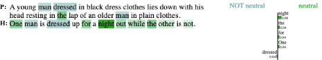
Figure 3: LIME saliency map highlighting the top feature words in the BERT model’s prediction. The top figure shows that the occurrence of ‘not’ causes BERT trained on counterfactual augmentation to misclassify the example as contradiction, verifying the spurious pattern of associating negation with the contradiction class that is uncovered by kNN in Table 2 (bottom block). The bottom figure shows the contrast that before augmentation the model did not not have those spurious associations and so was able to make the right prediction (neutral).

• Identifying mislabeled examples. Datasets used for training deep learning models are huge and may contain noisy labels depending on how the data was collected. Even crowd-sourced datasets can sometimes have mislabeled examples (Frénay and Verleysen 2013). $K$NN can be leveraged for identifying potentially mislabeled examples. We observed that $k$NN would sometimes retrieve mislabeled examples, and that these specific instances tended to occur when $k$NN’s prediction was different from the models prediction.

We experimented with this phenomenon by intentionally mislabeling 10% of examples on the original training split of the SNLI dataset with 1666 examples, and using $k$NN  based method to recover them by comparing with the model’s prediction as follows (based on the notations used in Section Method):

$$\operatorname*{arg\,max}p_{\theta}(y|x^{\prime})\neq\operatorname*{arg\,max}p_{knn}(y|x^{\prime})$$

We collected a set of candidate mislabeled training examples by comparing BERT’s prediction on the dev set to the label of the immediate nearest neighbor ($k$=1) for that example. We found that our approach was extremely effective at identifying the mislabeled examples with both high precision and recall. We obtained precision, recall and F1 of $0.84$, $0.73$, and $0.78$ respectively averaged over three random seeds.

We compared our results to a baseline that classifies training examples with the highest training loss as potentially mislabeled. Figure 4 shows a plot of the baseline with respect to the fraction of training data and the corresponding recall. Because our approach retrieves a set of candidate examples and there is no ranking, we directly plot the performance based on the size of the set. Our results indicate that $k$NN is extremely effective at identifying the mislabeled examples compared to the baseline that requires about 65% of the training data ranked by loss to get to the same performance. We applied our approach to the counterfactually augmented split of SNLI and found that our method effectively uncovers several mislabeled examples as shown in Table 3.

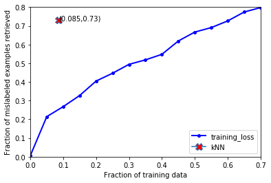
Figure 4: Fraction of correctly retrieved mislabeled examples by our $k$NN approach compared to a baseline that considers examples with highest training loss as mislabeled. Our approach has high recall while retrieving a significantly smaller set of candidate mislabeled examples.

P: A person uses their laptop. H: A person uses his laptop in his car.   GT: [entailment]

P: A man in a white shirt at a stand surrounded by beverages and lots of lemons. H: The man is selling food.   GT: [contradiction]

P: Extreme BMX rider with no gloves and completing a jump. H: A bike rider has biking gloves.   GT: [contradiction]

P: A family is observing a flying show. H: A family looking up into the sky at a flight show outside.   GT: [entailment]

P: A man is riding a motorcycle with a small child sitting in front of him. H: A man rides his motorcyle with his won.   GT: [entailment]

P: A man is riding a blue truck with a small child sitting in front of him. H: A man rides his motorcyle with his won.   GT: [contradiction]

P: A girl jumping into a swimming pool. H: A girl is taking a swim outside.   GT: [entailment]

P: A young woman wearing a black tank top is listening to music on her MP3 player while standing in a crowd. H: A young woman decided to leave home.  GT: [entailment]

Table 3: Random sample of retrieved candidate mislabeled examples from the SNLI augmented split. Not all are mislabeled and some also have mispelled words.

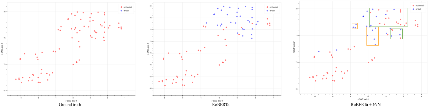
Figure 5: Visualization of RoBERTa’s representation using t-SNE on a small subset of the HANS constituent heuristic portion of the val set. Because $k$NN is highly non-linear, it is able to recover from some of the misclassifications of RoBERTa (highlighted using green box) for the difficult non-entail class. It makes the performance slightly worse on much smaller clusters (highlighted using orange box).

Apart from explaining model behavior and identifying mislabeled examples, we explore mechanisms for leveraging $k$NN to further improve fine-tuned model predictions described in the next section. • $K$NN for improving model performance. $K$NN has the ability to learn a highly non-linear boundary and so we leverage it to improve performance of fine-tuned models on examples which we know the model is not good at classifying. We deploy $k$NN as a backoff for low confidence predictions by learning a threshold on the validation set, below which the model’s predictions are very unreliable. Another criteria could be defining slices of data that satisfy a property on which the model is known to perform poorly. Examples include inputs that contain gendered words or fallible patterns for a model.

	SNLI		ANLI	HANS
	Original	Augmented
	$k$=16	$k$=16	$k$=64	$k$=64
BERT	$75.7$	$70.5$	$47.2$	$52.4$
$k$NN- BERT	$75.8$	$71.0$	$48.5$	$52.4$
RoBERTa	$82.8$	$76.8$	$44.4$	$59.3$
$k$NN-RoBERTa	$82.8$	$77.3$	$47.9$	$59.6$

Table 4: Results on NLI test sets for BERT and RoBERTa compared to $k$NN used along with the underlying model. Numbers indicate accuracy. SNLI and ANLI are 3-way classification tasks while HANS is a 2-way classification task.

Results on NLI.

For all our experiments we used $k$NN as a backoff for examples where the underlying fine-tuned model has low confidence in its prediction. These thresholds are identified on the validation splits for each of the evaluation datasets. We also experimented with different values of $k$ ($<1\%$ of the size of training data) and the temperature T for different training data sizes.

Dataset	BERT	RoBERTa
SNLI original	0.74	0.55
SNLI augmented	0.53	0.40
ANLI	0.95	0.96
HANS	0.84	0.62

Table 5: Threshold $\tau$ used for switching to $k$NN identified on the validation sets.

Table 4 shows the performance of BERT and RoBERTa with and without $k$NN on the overall test set for three NLI datasets. Our method of combining $k$NN with the underlying model obtains beats the standard BERT/RoBERTa with big margins on both augmented SNLI and ANLI. We also observe slight improvements on some of the other datasets.

To get a better insight into how $k$NN improves the fine-tuned models, we visualized RoBERTa’s learned representations over a sample of the HANS validation set. The sample is chosen from the particularly difficult constituent heuristic of HANS that assumes that a premise entails all complete sub-trees in its parse tree (McCoy, Pavlick, and Linzen 2019). Figure 5 illustrates how the predictions change when using just fine-tuned RoBERTa vs. in combination with $k$NN. Our approach does particularly well on the more difficult not-entail class as identified by McCoy, Pavlick, and Linzen (2019). Fine-grained quantitative results shows in Table 6. We used t-SNE (Maaten and Hinton 2008) to project the representations into two dimensions for visualization.

	Lexical overlap	Subsequence	Constituent
BERT	23.3	30.6	18.2
$k$NN- BERT	25.4	30.6	24.6
RoBERTa	78.7	79.6	52.7
$k$NN-RoBERTa	79.4	80.8	54.7

Table 6: Fine-grained performance on HANS test set for the more difficult not-entail class. $k$NN consistently outperforms the underlying model by itself.

Analysis.

Our experiments indicate that $k$NN can improve the performance of state-of-the-art models especially on input types on which the model is known to perform poorly. In this paper, we only considered the model’s low confidence as an indicator for switching to $k$NN. The backoff criteria could be anything that is based on the input examples. Slicing the datasets based on the occurrence of certain patterns in the input text like mention of colors or criterion based on syntactic information such as part-of-speech tags or lexical overlap can give a deeper understanding of model behavior. Fine-grained evaluations on such slices on a validation set would highlight data slices where the model performs poorly. Example types that satisfy these criterion can then be classified by switching to $k$NN for the final prediction.

Based on our application of $k$NN for uncovering spurious associations, it is evident that high performance on data augmentation such as counterfactuals that are not targeted for pre-defined groups or patterns in examples does not indicate robustness on all slices of data (e.g. examples with the ‘not’ pattern). It is difficult to make any claims about robustness without performing fine-grained analysis using data slices. On the other hand, targeted augmentation techniques such as HANS work better for evaluating robustness on the pre-defined syntactic heuristic categories.

Conclusion and future directions

We leveraged $k$NN over hidden representations to study the behavior of NLI models, and find that this approach is useful both for interpretability and improving model performance. We find that the $k$NN for any test example can give useful information about how a model makes its classification decisions. This is especially valuable for studying where models go wrong, and we demonstrate how retrieving the nearest neighbors can reveal artifacts and spurious correlations that cause models to misclassify examples.

From our analysis, we also observed that $k$NN of misclassified test examples are often indicative of mislabeled examples, which gives this approach application to fixing mislabeled examples in training sets. By finding the most common nearest neighbors across the whole test set, we are also able to identify a subset of highly influential training examples and obtain corpus-level interpretability for the model’s performance.

Lastly, we examined the utility of backing off to $k$NN-based classification when the model confidence is low. Analysis of the decision boundaries learned by $k$NN over hidden representations suggest that kNN learns a more fine-grained decision boundary that could help make it more robust to small changes in text that cause the ground truth label, but not the model prediction, to flip. We find that this approach increases the robustness of models to adversarial NLI datasets.

Future work could extend the effectiveness of $k$NN to other applications such as identifying domain mismatch between training and test or finding the least influential examples in a training set. Other directions include extending $k$NN to other classification tasks as well as generation.

References

- Alvarez-Melis and Jaakkola (2017) Alvarez-Melis, D.; and Jaakkola, T. 2017. A causal framework for explaining the predictions of black-box sequence-to-sequence models. In Proceedings of EMNLP, 412–421.
- Bastings, Aziz, and Titov (2019) Bastings, J.; Aziz, W.; and Titov, I. 2019. Interpretable Neural Predictions with Differentiable Binary Variables. In Proceedings of the 57th Annual Meeting of the Association for Computational Linguistics, 2963–2977. Florence, Italy: Association for Computational Linguistics. doi:10.18653/v1/P19-1284. URL https://www.aclweb.org/anthology/P19-1284.
- Bowman et al. (2015) Bowman, S. R.; Angeli, G.; Potts, C.; and Manning, C. D. 2015. A large annotated corpus for learning natural language inference. In Proceedings of EMNLP, 632–642.
- Brunner et al. (2020) Brunner, G.; Liu, Y.; Pascual, D.; Richter, O.; Ciaramita, M.; and Wattenhofer, R. 2020. On Identifiability in Transformers. In International Conference on Learning Representations. URL https://openreview.net/forum?id=BJg1f6EFDB.
- Chang et al. (2019) Chang, S.; Zhang, Y.; Yu, M.; and Jaakkola, T. 2019. A Game Theoretic Approach to Class-wise Selective Rationalization. In Advances in Neural Information Processing Systems, 10055–10065.
- Dagan, Glickman, and Magnini (2005) Dagan, I.; Glickman, O.; and Magnini, B. 2005. The PASCAL recognising textual entailment challenge. In Machine Learning Challenges Workshop, 177–190. Springer.
- Devlin et al. (2018) Devlin, J.; Chang, M.-W.; Lee, K.; and Toutanova, K. 2018. Bert: Pre-training of deep bidirectional transformers for language understanding. arXiv preprint arXiv:1810.04805 .
- Frénay and Verleysen (2013) Frénay, B.; and Verleysen, M. 2013. Classification in the presence of label noise: a survey. IEEE transactions on neural networks and learning systems 25(5): 845–869.
- Grave, Cisse, and Joulin (2017) Grave, E.; Cisse, M. M.; and Joulin, A. 2017. Unbounded cache model for online language modeling with open vocabulary. In Advances in Neural Information Processing Systems, 6042–6052.
- Grave, Joulin, and Usunier (2017) Grave, E.; Joulin, A.; and Usunier, N. 2017. Improving neural language models with a continuous cache. ICLR .
- Gu et al. (2018) Gu, J.; Wang, Y.; Cho, K.; and Li, V. O. 2018. Search engine guided neural machine translation. In Thirty-Second AAAI Conference on Artificial Intelligence.
- Gururangan et al. (2018) Gururangan, S.; Swayamdipta, S.; Levy, O.; Schwartz, R.; Bowman, S. R.; and Smith, N. A. 2018. Annotation artifacts in natural language inference data. arXiv preprint arXiv:1803.02324 .
- Han, Wallace, and Tsvetkov (2020) Han, X.; Wallace, B. C.; and Tsvetkov, Y. 2020. Explaining Black Box Predictions and Unveiling Data Artifacts through Influence Functions. arXiv preprint arXiv:2005.06676 .
- Ioffe and Szegedy (2015) Ioffe, S.; and Szegedy, C. 2015. Batch normalization: Accelerating deep network training by reducing internal covariate shift. arXiv preprint arXiv:1502.03167 .
- Jain and Wallace (2019) Jain, S.; and Wallace, B. C. 2019. Attention is not Explanation. In Proceedings of the NAACL, 3543–3556.
- Johnson, Douze, and Jégou (2019) Johnson, J.; Douze, M.; and Jégou, H. 2019. Billion-scale similarity search with GPUs. IEEE Transactions on Big Data .
- Kaushik, Hovy, and Lipton (2020) Kaushik, D.; Hovy, E.; and Lipton, Z. 2020. Learning The Difference That Makes A Difference With Counterfactually-Augmented Data. In International Conference on Learning Representations. URL https://openreview.net/forum?id=Sklgs0NFvr.
- Khandelwal et al. (2020) Khandelwal, U.; Levy, O.; Jurafsky, D.; Zettlemoyer, L.; and Lewis, M. 2020. Generalization through Memorization: Nearest Neighbor Language Models. ICLR .
- Koh and Liang (2017) Koh, P. W.; and Liang, P. 2017. Understanding black-box predictions via influence functions. In Proceedings of ICML, 1885–1894. JMLR. org.
- Lei, Barzilay, and Jaakkola (2016) Lei, T.; Barzilay, R.; and Jaakkola, T. 2016. Rationalizing Neural Predictions. In Proceedings of EMNLP, 107–117.
- Li, Zhang, and Zong (2018) Li, X.; Zhang, J.; and Zong, C. 2018. One Sentence One Model for Neural Machine Translation. In Proceedings of the Eleventh International Conference on Language Resources and Evaluation (LREC-2018). Miyazaki, Japan: European Languages Resources Association (ELRA). URL https://www.aclweb.org/anthology/L18-1146.
- Liu et al. (2019) Liu, Y.; Ott, M.; Goyal, N.; Du, J.; Joshi, M.; Chen, D.; Levy, O.; Lewis, M.; Zettlemoyer, L.; and Stoyanov, V. 2019. Roberta: A robustly optimized bert pretraining approach. arXiv preprint arXiv:1907.11692 .
- Maaten and Hinton (2008) Maaten, L. v. d.; and Hinton, G. 2008. Visualizing data using t-SNE. Journal of machine learning research 9(Nov): 2579–2605.
- McCoy, Pavlick, and Linzen (2019) McCoy, R. T.; Pavlick, E.; and Linzen, T. 2019. Right for the wrong reasons: Diagnosing syntactic heuristics in natural language inference. arXiv preprint arXiv:1902.01007 .
- Nie et al. (2020) Nie, Y.; Williams, A.; Dinan, E.; Bansal, M.; Weston, J.; and Kiela, D. 2020. Adversarial NLI: A New Benchmark for Natural Language Understanding. In ACL.
- Papernot and McDaniel (2018) Papernot, N.; and McDaniel, P. 2018. Deep k-nearest neighbors: Towards confident, interpretable and robust deep learning. arXiv preprint arXiv:1803.04765 .
- Poliak et al. (2018) Poliak, A.; Naradowsky, J.; Haldar, A.; Rudinger, R.; and Van Durme, B. 2018. Hypothesis only baselines in natural language inference. arXiv preprint arXiv:1805.01042 .
- Pruthi et al. (2020) Pruthi, D.; Gupta, M.; Dhingra, B.; Neubig, G.; and Lipton, Z. C. 2020. Learning to Deceive with Attention-Based Explanations. In Annual Conference of the Association for Computational Linguistics (ACL). URL https://arxiv.org/abs/1909.07913.
- Reimers and Gurevych (2019) Reimers, N.; and Gurevych, I. 2019. Sentence-bert: Sentence embeddings using siamese bert-networks. arXiv preprint arXiv:1908.10084 .
- Ribeiro, Singh, and Guestrin (2016) Ribeiro, M. T.; Singh, S.; and Guestrin, C. 2016. “ Why should i trust you?” Explaining the predictions of any classifier. In Proceedings of the 22nd ACM SIGKDD international conference on knowledge discovery and data mining, 1135–1144.
- Ribeiro, Singh, and Guestrin (2018) Ribeiro, M. T.; Singh, S.; and Guestrin, C. 2018. Anchors: High-precision model-agnostic explanations. In Thirty-Second AAAI Conference on Artificial Intelligence.
- Serrano and Smith (2019) Serrano, S.; and Smith, N. A. 2019. Is Attention Interpretable? In Proceedings of the 57th Annual Meeting of the Association for Computational Linguistics, 2931–2951. Florence, Italy: Association for Computational Linguistics. doi:10.18653/v1/P19-1282. URL https://www.aclweb.org/anthology/P19-1282.
- Singh and Anand (2018) Singh, J.; and Anand, A. 2018. Exs: Explainable search using local model agnostic interpretability. arXiv preprint arXiv:1809.03857 .
- Vaswani et al. (2017) Vaswani, A.; Shazeer, N.; Parmar, N.; Uszkoreit, J.; Jones, L.; Gomez, A. N.; Kaiser, L.; and Polosukhin, I. 2017. Attention is All you Need. In NeurIPS, 5998–6008.
- Weston, Dinan, and Miller (2018) Weston, J.; Dinan, E.; and Miller, A. H. 2018. Retrieve and refine: Improved sequence generation models for dialogue. arXiv preprint arXiv:1808.04776 .
- Wiegreffe and Pinter (2019) Wiegreffe, S.; and Pinter, Y. 2019. Attention is not not Explanation. In Proceedings of the 2019 Conference on Empirical Methods in Natural Language Processing and the 9th International Joint Conference on Natural Language Processing (EMNLP-IJCNLP), 11–20. Hong Kong, China: Association for Computational Linguistics. doi:10.18653/v1/D19-1002. URL https://www.aclweb.org/anthology/D19-1002.
- Williams, Nangia, and Bowman (2018) Williams, A.; Nangia, N.; and Bowman, S. 2018. A Broad-Coverage Challenge Corpus for Sentence Understanding through Inference. In Proceedings of NAACL, 1112–1122.
- Zhang et al. (2019) Zhang, T.; Kishore, V.; Wu, F.; Weinberger, K. Q.; and Artzi, Y. 2019. Bertscore: Evaluating text generation with bert. arXiv preprint arXiv:1904.09675 .
- Zhao et al. (2020) Zhao, M.; Wu, H.; Niu, D.; and Wang, X. 2020. Reinforced Curriculum Learning on Pre-trained Neural Machine Translation Models. arXiv preprint arXiv:2004.05757 .
- Zhong, Shao, and McKeown (2019) Zhong, R.; Shao, S.; and McKeown, K. 2019. Fine-grained Sentiment Analysis with Faithful Attention. arXiv preprint arXiv:1908.06870 .