A Framework to Quantify Approximate Simulation on Graph Data

Abstract

Simulation and its variants (e.g., bisimulation and degree-preserving simulation) are useful in a wide spectrum of applications. However, all simulation variants are coarse “yes-or-no” indicators that simply confirm or refute whether one node simulates another, which limits the scope and power of their utility. Therefore, it is meaningful to develop a fractional $\chi$-simulation measure to quantify the degree to which one node simulates another by the simulation variant $\chi$. To this end, we first present several properties necessary for a fractional $\chi$-simulation measure. Then, we present ${\mathsf{FSim}}_{\chi}$, a general fractional $\chi$-simulation computation framework that can be configured to quantify the extent of all $\chi$-simulations. Comprehensive experiments and real-world case studies show the measure to be effective and the computation framework to be efficient.

1 Introduction

Consider two directed graphs $G_{1}$ and $G_{2}$ with labeled nodes from the sets $V_{1}$ and $V_{2}$, respectively. A simulation [1] relation $R\subseteq V_{1}\times V_{2}$ is a binary relation over $V_{1}$ and $V_{2}$. For each node pair $(u,v)$ in $R$ (namely, $u$ is simulated by $v$), each $u$’s out-neighbor is simulated by one of $v$’s out-neighbors, and the same applies to in-neighbors. An illustration of this concept is shown below.

Example 1.

As shown in Figure 1, node $u$ is simulated by node $v_{2}$, as they have the same label, and each $u$’s out-neighbor can be simulated by the same-label out-neighbor of $v_{2}$ ($u$ has no in-neighbors). Note that the two hexagonal nodes in $\mathcal{P}$ are simulated by the same hexagonal node in $\mathcal{G}_{2}$. Similarly, $u$ is simulated by $v_{3}$ and $v_{4}$. However, $u$ can not be simulated by $v_{1}$, as the pentagonal neighbor of $u$ cannot be simulated by any neighbor of $v_{1}$.

The original definition of simulation put forward by Milner in 1971 [2] only considered out-neighbors. But, in 2011, Ma et al. [1] revised the definition to consider in-neighbors, making it capture more topological information. Additionally, different variants of simulation have emerged over the years, each with its own constraint(s). For example, on the basis that $R$ is a simulation relation, bisimulation [3] further requires that $R^{-1}$ is also a simulation, where $R^{-1}$ denotes the converse relation of $R$ (i.e., $R^{-1}=\{(v,u)|\forall(u,v)\in R\}$); and degree-preserving simulation [4] requires that two neighbors of $u$ cannot be simulated by the same neighbor of $v$.

Applications. Simulation and its variants are important relations among nodes, and have been adopted in a wide range of applications. For example, simulation and degree-preserving simulation are shown to be effective in graph pattern matching [5, 1, 6, 4], and a node in the data graph is considered to be a potential match for a node in the query graph if it simulates the query node. Bisimulation has been applied to compute RDF graph alignment [7] and graph partition [8, 9, 10]. Generally, two nodes will be aligned or be placed in the same partition if they are in a bisimulation relation. Other applications include data retrieval [11], graph compression [12] and index construction [13, 14, 15], etc.

Figure 1: Example graphs. A node’s shape denotes its label.

Motivations. Despite their numerous valuable uses, simulation and its variants are all coarse “yes-or-no” indicators. That is, simulation and its variants can only answer whether node $v$ can fully simulate node $u$; they cannot tell us whether $v$ might be able to partially or even very nearly (i.e., approximately) simulate $u$. This coarseness raises two practical issues. First, there often exist some nodes that nearly simulate $u$ in real-world graphs, which either naturally present in the graphs or are consequences of data errors (a common issue by data noise and mistakes of collecting data). However, simulation and its variants cannot catch these nodes and cause loss of potential results. Second, the coarseness makes it inappropriate to apply simulation and its variants to applications that naturally require fine-grained evaluation, such as node similarity measurement. Example 2 provides a real-life illustration of these issues.

Example 2.

We consider the application of simulation to determine whether or not a poster $A$ is simulated by another poster $B$ in terms of their design elements (e.g., color, layout, font, and structure). For example, when compared with the poster $P_{1}$ in Figure 2(b), the candidate poster $P$ in Figure 2(a) only slightly differs in the font and font style. Hence, it is highly suspected as a case of plagiarism [16]. Nevertheless, due to a minor change of design elements, there is no exact simulation relation between posters $P$ and $P_{1}$, and thus exact simulation can not be used to discover such similarity. As a result, it is more desirable to develop a mechanism to capture the similarity between two posters via the degree of approximate simulation (some fine-grained measurement), instead of simply using the exact simulation.

(a) A poster

(b) A database of existing posters

(c) Query graph

(d) Data graph

Figure 2: Motivating example. Figures (c) and (d) are graphs representing the posters in (a) and (b), respectively. Nodes are marked with their labels. An edge from nodes u to v indicates that the poster u has a design element v.

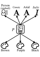
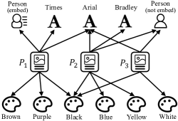
In general, it is of practical need to develop a mechanism to quantify the cases of approximate simulation to remedy the impacts of the “yes-or-no” semantics. Such quantification can not only open up a host of possibilities for using simulation but also make the results of simulation more effective and robust. Although the simulation variants differ in certain properties, they are actually derived from a common foundation, namely the simulation relation [2]. Consequently, instead of developing a quantification technique independently and individually for each variant, it is more desirable to devise a general framework that works for all simulation variants. Aside from the obvious benefits of less redundancy, developing a unified framework requires a systematic study of the properties of the different simulation variants. Not only has this not been done before, doing so may help to inspire new variants.

Our Contributions. We propose the fractional $\chi$-simulation framework that quantifies the extent of simulation and its variants in the range of $[0,1]$. Our main contributions are as follows.

(1) A unified definition of $\chi$-simulation. From a systematic study of the properties of simulation and its variants, we distill the base definition of simulation and its variants into a unified definition called $\chi$-simulation. Further, we discover and name a new simulation variant - bijective simulation. Theoretically, bijective simulation is akin to the well-known Weisfeiler-Lehman isomorphism test [17] (Section 4.3). Practically, its fractional form (contribution 2) is more effective than the existing models regarding node similarity measurement, as detailed in Section 5.4.

(2) A general framework ${\mathsf{FSim}}_{\chi}$ for computing fractional $\chi$-simulation. To quantify the degree to which one node simulates another by a $\chi$-simulation, we propose the concept of fractional $\chi$-simulation and identify a list of properties that a fractional $\chi$-simulation measure should satisfy. Then, we present a general computation framework, namely ${\mathsf{FSim}}_{\chi}$, which can be configured to compute fractional $\chi$-simulation for all $\chi$-simulations with the properties satisfied. ${\mathsf{FSim}}_{\chi}$ is an iterative framework that computes the fractional $\chi$-simulation scores for all pairs of nodes over two graphs. Furthermore, we show the relations of ${\mathsf{FSim}}_{\chi}$ to several well-known concepts, including node similarity measures (i.e., $\mathsf{SimRank}$ [18] and $\mathsf{RoleSim}$ [19]) and an approximate variant of bisimulation (i.e., $k$-bisimulation [20, 21, 22, 10]), in Section 4.3.

(3) Extensive experiments and case studies. We perform empirical studies to exhibit that ${\mathsf{FSim}}_{\chi}$ is robust to parameter tuning and data errors, and is efficient to compute on real-world graphs. We further conduct three case studies to evaluate ${\mathsf{FSim}}_{\chi}$’s potential for subgraph pattern matching, node similarity measurement, and RDF graph alignment. Based on these studies, we reach the following conclusions. First, fractional $\chi$-simulation can remedy the “yes-or-no" semantics of $\chi$-simulation, and it significantly improves the effectiveness of $\chi$-simulation in the related applications, e.g., simulation in subgraph pattern matching. Second, fractional bijective simulation (proposed in this paper) is a highly effective way of measuring node similarity. Finally, the ${\mathsf{FSim}}_{\chi}$ framework provides a flexible way to study the effectiveness of different simulation variants, and thus can be used as a tool to help identify the best variant for a specific application.

2 Simulation and Its Variants

Data Model. Consider a node-labeled directed graph $G=(V,E,\ell)$, where $V(G)$ and $E(G)$ denote the node set and edge set, respectively (or $V$ and $E$ when the context is clear). $\Sigma$ is a set of string labels, and $\ell:V\rightarrow\Sigma$ is a labeling function that maps each node $u$ to a label $\ell(u)\in\Sigma$. $N_{G}^{+}(u)=\{u^{\prime}|(u,u^{\prime})\in E(G)\}$ denotes node $u$’s out-neighbors and, likewise, $N_{G}^{-}(u)=\{u^{\prime}|(u^{\prime},u)\in E(G)\}$ denotes its in-neighbors. Let $d_{G}^{+}(u)=|N_{G}^{+}(u)|$ and $d_{G}^{-}(u)=|N_{G}^{-}(u)|$ be the out- and in-degrees of node $u$, and let $d_{G}$, $D^{+}_{G}$ and $D^{-}_{G}$ denote the average degree, maximum out-degree and maximum in-degree of $G$, respectively. A summary of the notations used throughout this paper appears in Table 1.

Table 1: Table of Notations

Notation	Description
$G=(V,E,\ell)$	a node-labeled directed graph
$V(G)/E(G)$	the node/edge set of graph $G$
$\ell(\cdot)$	a labeling function
$N_{G}^{+}(u)/N_{G}^{-}(u)$	the out-neighbors/in-neighbors of node $u$ in $G$
$d_{G}^{+}(u)/d_{G}^{-}(u)$	the out-degree/in-degree of node $u$ in $G$
$d_{G}$	the average degree of $G$
$D^{+}_{G}/D^{-}_{G}$	the maximum out-degree/in-degree of $G$

Simulation Variants. The first step in developing a unified definition of simulation and its variants is to formally define simulation as the foundation of all its variants.

Definition 1.

(Simulation) Given the graphs $G_{1}=(V_{1},E_{1},\ell_{1})$ and $G_{2}=(V_{2},E_{2},\ell_{2})$, a binary relation $R\subseteq V_{1}\times V_{2}$ is a simulation if, for $\forall(u,v)\in R$, it satisfies that:

1. $\ell_{1}(u)=\ell_{2}(v)$,

2. $\!\forall u^{\prime}\in N_{G_{1}}^{+}(u)$, $\!\exists v^{\prime}\in N_{G_{2}}^{+}(v)\!$ such that (s.t.) $(u^{\prime},v^{\prime})\in R$,

3. $\forall u^{\prime\prime}\in N_{G_{1}}^{-}(u)$, $\exists v^{\prime\prime}\in N_{G_{2}}^{-}(v)$ s.t. $(u^{\prime\prime},v^{\prime\prime})\in R$.

For clarity, $u$ is always a node from $V_{1}$, and $v$ is always a node from $V_{2}$ in this paper.

The variants of simulation are based on Definition 1 but have additional constraints. Definition 2 below provides a summary of several common simulation variants. However, one exceptional variant, strong simulation [1], must be discussed first. Strong simulation is designed for subgraph pattern matching. In brief, strong simulation exists between the query graph $Q$ and data graph $G$ if a subgraph $G[v,\delta_{Q}]$ of $G$ satisfies the following criteria: (1) a simulation relation $R$ exists between $Q$ and $G[v,\delta_{Q}]$; and (2) $R$ contains node $v$ and all nodes in $Q$. Note that the subgraph $G[v,\delta_{Q}]$ is an induced subgraph that includes all nodes whose shortest distances to $v$ in $G$ are not larger than the diameter $\delta_{Q}$ of $Q$. In essence, strong simulation essentially performs simulation (Definition 1) multiple times, and so does not need to be specifically defined or further discussed.

Definition 2, which follows, shows how $\chi$-simulation summarizes the base definition of simulation but also considers its variants. The definition below includes two notable ones in degree-preserving simulation [4] and bisimulation [3].

Definition 2.

($\chi$-simulation) A simulation relation $R$ by Definition 1 is further a $\chi$-simulation relation, which corresponds to

• Simulation ($\chi={\mathsf{s}}$): no extra constraint;

• Degree-preserving simulation ($\chi={\mathsf{dp}}$): if $(u,v)\in R$, (1) there exists an injective function $\lambda_{1}:N_{G_{1}}^{+}(u)\to N_{G_{2}}^{+}(v)$, s.t. $\forall u^{\prime}\in N_{G_{1}}^{+}(u)$, $(u^{\prime},\lambda_{1}(u^{\prime}))\in R$; and (2) there exists an injective function $\lambda_{2}:N_{G_{1}}^{-}(u)\to N_{G_{2}}^{-}(v)$, s.t. $\forall u^{\prime\prime}\in N_{G_{1}}^{-}(u)$, $(u^{\prime\prime},\lambda_{2}(u^{\prime\prime}))\in R$;

• Bisimulation ($\chi$ = $\mathsf{b}$): if $(u,v)\in R$, (1) $\forall v^{\prime}\in N^{+}(v)$, $\exists u^{\prime}\in N^{+}(u)$ s.t. $(u^{\prime},v^{\prime})\in R$; and (2) $\forall v^{\prime\prime}\in N^{-}(v)$, $\exists u^{\prime\prime}\in N^{-}(u)$ s.t. $(u^{\prime\prime},v^{\prime\prime})\in R$.

Node $u$ is $\chi$-simulated by node $v$ (or $v$ $\chi$-simulates $u$), denoted as $u\rightsquigarrow^{\chi}v$, if there is a $\chi$-simulation relation $R$ with $(u,v)\in R$. Specifically, if $u\rightsquigarrow^{\chi}v$ implies $v\rightsquigarrow^{\chi}u$ (i.e., $\chi={\mathsf{b}}$), we may use $u\sim^{\chi}v$ directly.

Example 3.

Recall that in Example 1, $u$ is simulated by nodes $v_{2}$, $v_{3}$ and $v_{4}$ in Figure 1. However, $u$ cannot be ${\mathsf{dp}}$-simulated by $v_{2}$. This is because $u$ has two hexagonal neighbors and $v_{2}$ does not, which contradicts the requirement of “injective function”; Analogously, $u$ cannot be ${\mathsf{b}}$-simulated by $v_{3}$, since $v_{3}$’s square neighbor fails to simulate any neighbor of $u$.

Inspired by the constraints of ${\mathsf{dp}}$- and ${\mathsf{b}}$-simulations, we find that a $\chi$-simulation may have the following properties: (1) injective neighbor mapping (or IN-mapping for short), i.e., $\forall(u,v)\in R$, two different neighbors (either in or out) of $u$ cannot be mapped to the same neighbor of $v$; and (2) converse invariant, i.e., where $R^{-1}=\{(v,u)|\forall(u,v)\in R\}$ is a $\chi$-simulation if $R$ is a $\chi$-simulation. By Definition 2, ${\mathsf{dp}}$-simulation has the property of IN-mapping, while ${\mathsf{b}}$-simulation has converse invariant. The properties of the exiting simulation variants are listed in Figure 3(a).

Remark 1.

Given a $\chi$-simulation with the property of converse invariant, if $u\rightsquigarrow^{\chi}v$, then $v\rightsquigarrow^{\chi}u$ must hold. Therefore, in Definition 2, we have $u\rightsquigarrow^{{\mathsf{b}}}v$ implies $v\rightsquigarrow^{{\mathsf{b}}}u$.

Figure 3: The summarization of all simulation variants.

A New Variant: Bijective Simulation. In compiling Figure 3(a), we realize that no simulation variant had both IN-mapping and converse invariant. This motivated us to define one. Called bijective simulation, our definition follows.

Definition 3.

(Bijective Simulation) A simulation relation $R\subseteq V_{1}\times V_{2}$ is a bijective simulation ($\chi={\mathsf{bj}}$), if $R$ is a degree-preserving simulation and the functions $\lambda_{1}$ and $\lambda_{2}$, as defined in Definition 2, are further to be surjective (i.e., $\lambda_{1}$ and $\lambda_{2}$ are bijective). Bijective simulation is considered in the $\chi$-simulation (Definition 2) by letting $\chi={\mathsf{bj}}$.

Compared to ${\mathsf{dp}}$-simulation, ${\mathsf{bj}}$-simulation requires that the mapping functions of the neighbors to be bijective. In other words, each pair of neighbors in a ${\mathsf{bj}}$-simulation must be mapped one by one. It’s not hard to verify that ${\mathsf{bj}}$-simulation has the properties of both IN-mapping and converse invariance.

Figure 3(b) shows the strictness among the simulation variants, where a “more-strict” edge from a $\chi_{1}$- to a $\chi_{2}$-simulation means that the $\chi_{1}$-simulation must also be a $\chi_{2}$-simulation. Such strictness among the variants can also be inferred from Figure 1. More specifically, given $u\rightsquigarrow^{{\mathsf{bj}}}v_{4}$, it holds that $u\rightsquigarrow^{\chi}v_{4}$, $\forall\chi\in\{{\mathsf{s}},{\mathsf{b}},{\mathsf{dp}}\}$.

Summary. In this paper, we consider all together four simulation variants: simulation ($\chi={\mathsf{s}}$), degree-preserving simulation ($\mathsf{dp}$), bisimulation ($\mathsf{b}$), and bijective simulation ($\mathsf{bj}$). With a systematic study of existing simulation variants, we have discovered bijective simulation as a new variant. We believe that our work will further inspire more variants.

Hereafter, we may omit the $\chi$ in $\chi$-simulation, referring simply to simulation. To avoid ambiguity, we call the simulation relation in Definition 1 as simple simulation.

3 Fractional Simulation

To quantify the degree to which one node simulates the other node, we now set out the properties fractional $\chi$-simu-lation should satisfy and the framework for its computation.

3.1 The Properties of Fractional Simulation

Definition 4.

(Fractional $\chi$-Simulation) Given graphs $G_{1}=(V_{1},E_{1},\ell_{1})$ and $G_{2}=(V_{2},E_{2},\ell_{2})$, and two nodes $u\in V_{1}$ and $v\in V_{2}$, the fractional $\chi$-simulation of $u$ and $v$ quantifies the degree to which $u$ is approximately $\chi$-simulated by $v$, denoted as ${\mathsf{FSim}}_{\chi}(u,v)$. ${\mathsf{FSim}}_{\chi}(u,v)$ should satisfy:

1. Range: $0\leq{\mathsf{FSim}}_{\chi}(u,v)\leq 1$;

2. Simulation definiteness: $u$ is $\chi$-simulated by $v$, i.e., $u{\rightsquigarrow}^{\chi}v$, if and only if ${\mathsf{FSim}}_{\chi}(u,v)=1$;

3. $\chi$-conditional symmetry: if the $\chi$-simulation has the property of converse invariant (i.e., $u\rightsquigarrow^{\chi}v$ implies $v\rightsquigarrow^{\chi}u$), then ${\mathsf{FSim}}_{\chi}(u,v)$ should be symmetric, i.e., ${\mathsf{FSim}}_{\chi}(u,v)={\mathsf{FSim}}_{\chi}(v,u)$.

A computation scheme ${\mathsf{FSim}}_{\chi}$ is well-defined for fractional $\chi$-simulation, if for $\forall(u,v)\in V_{1}\times V_{2}$, ${\mathsf{FSim}}_{\chi}(u,v)$ satisfies all three of the above properties.

Property 1 is a common practice. Property 2 bridges the fractional simulation and the corresponding simulation variant. The sufficient condition reflects the fact that $u$ being $\chi$-simulated by $v$ stands for the maximum degree of their simulation, while the necessary condition (only if) makes fractional simulation imply the case of simulation. Property 3 means the variants with converse invariance (i.e., bisimulation and bijective simulation) can be used as similarity measures.

3.2 Framework to Compute Fractional Simulation

We propose the ${\mathsf{FSim}}_{\chi}$ framework to compute the fractional $\chi$-simulation scores for all pairs of nodes across two graphs. The ${\mathsf{FSim}}_{\chi}$ is a non-trivial framework because it needs to account for the properties of all simulation variants as well as convergence in general. Note that hereafter, we use ${\mathsf{FSim}}_{\chi}$ interchangeably to indicate the framework and a $\chi$-simulation value.

Recall from Definition 2 that a node $u$ is $\chi$-simulated by node $v$ if they have the same label, and their neighbors are $\chi$-simulated accordingly. Thus, we have divided the computation of ${\mathsf{FSim}}_{\chi}(u,v)$ into three parts as follows:

$$\begin{split}{{\mathsf{FSim}}_{\chi}}(u,v)=\underbrace{w^{+}\text{ }{\mathsf{FSim}}_{\chi}(N_{G_{1}}^{+}(u),N_{G_{2}}^{+}(v))}_{\textbf{score by out-neighbors}}+\underbrace{w^{-}\text{ }{\mathsf{FSim}}_{\chi}(N_{G_{1}}^{-}(u),N_{G_{2}}^{-}(v))}_{\textbf{score by in-neighbors}}+\underbrace{(1-{w^{+}}-{w^{-}})\text{ }\mathcal{L}(u,v)}_{\textbf{score by node label}},\end{split}$$ (1)

where $\!{\mathsf{FSim}}_{\chi}(N_{G_{1}}^{+}(u),N_{G_{2}}^{+}(v))\!$ and ${\mathsf{FSim}}_{\chi}(N_{G_{1}}^{-}(u),N_{G_{2}}^{-}(v))$ denote the scores contributed by the out- and in-neighbors of $u$ and $v$ respectively. $w^{+}$ and $w^{-}$ are weighting factors that satisfy $0\leq w^{+}<1$, $0\leq w^{-}<1$ and $0<w^{+}+w^{-}<1$; and $\mathcal{L}(\cdot)$ is a label function that evaluates the similarity of two nodes’ labels. Specifically, if there is no prior knowledge about the labels, $\mathcal{L}(\cdot)$ can be derived by a wide variety of string similarity functions, such as an indicator function, normalized edit distance, Jaro-Winkler similarity, etc. Alternatively, the user could specify/learn the similarities of the label semantics. Since the latter case is beyond the scope of this paper, in the following, we assume no prior knowledge about the labels.

In Equation 1, we need to compute the $\chi$-simulation score between two node sets $S_{1}$ and $S_{2}$ (the respective neighbors of each node pair). To do so, we derive:

$${\mathsf{FSim}}_{\chi}(S_{1},S_{2})=\frac{\sum_{(x,y)\in\mathcal{M}_{\chi}(S_{1},S_{2})}{{\mathsf{FSim}}_{\chi}}(x,y)}{\Omega_{\chi}(S_{1},S_{2})},$$ (2)

where $\Omega_{\chi}$ denotes the normalizing operator that returns a positive integer w.r.t. $S_{1}$ and $S_{2}$. $\mathcal{M}_{\chi}$ denotes the mapping operator, which returns a set of node pairs defined as:

$$\mathcal{M}_{\chi}(S_{1},S_{2};f_{\chi})=\{(x,y)\;|\;x\in X,y=f_{\chi}(x)\in Y\},$$

where $X\subseteq S_{1}\cup S_{2}$ and $Y\subseteq S_{1}\cup S_{2}$. $f_{\chi}:X\to Y$ is a function that is subject to certain constraints regarding the simulation variant $\chi$. These constraints include the domain and codomain of $f_{\chi}$, and the properties that $f_{\chi}$ should satisfy (e.g., that $f_{\chi}$ is an injective function). Note that, for clear presentation, $f_{\chi}$ is always omitted from the mapping operator. How $\mathcal{M}_{\chi}$ and $\Omega_{\chi}$ are configured to deploy different simulation variants for the framework is demonstrated in Section 4.

Table 2: Results of whether $u$ is simulated by $v_{i}$ ($i\in\{1,2,3,4\}$) in Figure 1 regarding each simulation variant ($\checkmark$ for yes, $\times$ for no) and the corresponding fractional scores (in bracket)

Variants	$(u,v_{1})$	$(u,v_{2})$	$(u,v_{3})$	$(u,v_{4})$
${\mathsf{s}}$-simulation	$\times$ (0.85)	$\checkmark$ (1.00)	$\checkmark$ (1.00)	$\checkmark$ (1.00)
${\mathsf{dp}}$-simulation	$\times$ (0.72)	$\times$ (0.85)	$\checkmark$ (1.00)	$\checkmark$ (1.00)
${\mathsf{b}}$-simulation	$\times$ (0.78)	$\checkmark$ (1.00)	$\times$ (0.93)	$\checkmark$ (1.00)
${\mathsf{bj}}$-simulation	$\times$ (0.72)	$\times$ (0.81)	$\times$ (0.94)	$\checkmark$ (1.00)

Example 4.

Table 2 shows the ${\mathsf{FSim}}_{\chi}$ scores for some of the node pairs in Figure 1 based on the definition of fractional $\chi$-simulation (Definition 4) and the ${\mathsf{FSim}}_{\chi}$ framework (Equation 1). We can observe that: (1) a pair $(u,v)$ where $u$ is not but very closely simulated by $v$ has a high ${\mathsf{FSim}}_{\chi}$ score, e.g., ${\mathsf{FSim}}_{\mathsf{bj}}(u,v_{3})$; (2) when $u$ is $\chi$-simulated by $v$, ${\mathsf{FSim}}_{\chi}(u,v)$ reaches a maximum value of 1, e.g., ${\mathsf{FSim}}_{\mathsf{b}}(u,v_{4})$, which conforms with the well-definiteness of ${\mathsf{FSim}}_{\chi}$.

According to Equation 1, the $\!{\mathsf{FSim}}_{\chi}\!$ score between two nodes depends on the ${\mathsf{FSim}}_{\chi}$ scores of their neighbors. This naturally leads to an iterative computation scheme. This iterative process is detailed in the next section along with how to guarantee its convergence.

3.3 Iterative Computation

Consider ${{\mathsf{FSim}}}_{\chi}^{k}(u,v)$, which denotes the $\chi$-simulation score of nodes $u$ and $v$ in the $k$-[th] iteration ($k\geq 1$), the mapping operator $\mathcal{M}_{\chi}^{k}$ and the normalizing operator $\Omega_{\chi}^{k}$ applied in the given iteration.

Initialization. As all simulation variants require an equivalence of node labels (Definition 1 and Definition 2), The ${\mathsf{FSim}}_{\chi}$ score is initially set to ${{\mathsf{FSim}}}_{\chi}^{0}(u,v)=\mathcal{L}(u,v)$ by default unless otherwise specified. When using such initialization, $\mathcal{L}(u,v)=1$ must be further constrained if, and only if, $\ell_{1}(u)=\ell_{2}(v)$, in order to guarantee that ${\mathsf{FSim}}_{\chi}$ is well-defined (Definition 4).

Iterative Update. According to Equation 1 and Equation 2, the simulation score in the $k$-[th] iteration for a node pair $(u,v)$ regarding $\chi$ is updated via the scores of previous iteration as:

$$\begin{split}{{\mathsf{FSim}}}_{\chi}^{k}(u,v)&=\frac{w^{+}\sum_{(x,y)\in\mathcal{M}^{k}_{\chi}(N_{G_{1}}^{+}(u),N_{G_{2}}^{+}(v))}{{\mathsf{FSim}}}_{\chi}^{k-1}(x,y)}{\Omega^{k}_{\chi}(N_{G_{1}}^{+}(u),N_{G_{2}}^{+}(v))}+\frac{w^{-}\sum_{(x,y)\in\mathcal{M}^{k}_{\chi}(N_{G_{1}}^{-}(u),N_{G_{2}}^{-}(v))}{{\mathsf{FSim}}}_{\chi}^{k-1}(x,y)}{\Omega^{k}_{\chi}(N_{G_{1}}^{-}(u),N_{G_{2}}^{-}(v))}\\ &+(1-{w^{+}}-{w^{-}})\mathcal{L}(u,v)\end{split}$$ (3)

Convergence. Below we show what conditions the mapping and normalizing operators should satisfy to guarantee Equation 3 converges. Specifically, the computation is considered to converge if $|{\mathsf{FSim}}_{\chi}^{k+1}(u,v)-{\mathsf{FSim}}_{\chi}^{k}(u,v)|<\epsilon$ for $\forall(u,v)\in V_{1}\times V_{2}$, in which $\epsilon$ is a small positive value. Note that the simulation subscript $\chi$ is omitted in the following theorem as it applies to all simulation variants.

Theorem 1.

The computation in Equation 3 is guaranteed to converge if in every iteration $k$, the following conditions are satisfied for any two node sets $S_{1}$ and $S_{2}$ in the mapping and normalizing operators:

1. $|\mathcal{M}^{k+1}(S_{1},S_{2})|=|\mathcal{M}^{k}(S_{1},S_{2})|$, and $\Omega^{k+1}(S_{1},S_{2})=\Omega^{k}(S_{1},S_{2})$.

2. $|\mathcal{M}^{k}(S_{1},S_{2})|\leq\Omega^{k}(S_{1},S_{2})$.

3. Subject to the function $f$, $\mathcal{M}^{k}(S_{1},S_{2})$ returns node pairs such that

   $$\sum_{(x,y)\in\mathcal{M}^{k}(S_{1},S_{2})}{{\mathsf{FSim}}}^{k-1}(x,y)\text{ is maximized.}$$

Proof.

Let $\delta^{k}(u,v)=|{\mathsf{FSim}}^{k}(u,v)-{\mathsf{FSim}}^{k-1}(u,v)|$ and $\Delta^{k}=\max_{(u,v)}\delta^{k}(u,v)$. To prove this theorem, we must show that $\Delta^{k}$ decreases monotonically, i.e., $\Delta^{k+1}<\Delta^{k}$.

Let $W^{k}(S_{1},S_{2})=\sum_{(x,y)\in\mathcal{M}^{k}(S_{1},S_{2})}{\mathsf{FSim}}^{k-1}(x,y)$. As the size of the mapping operator and the value of normalizing operator between $S_{1}$ and $S_{2}$ do not vary with $k$ (C1), we simply write $|\mathcal{M}(S_{1},S_{2})|$ and $\Omega(S_{1},S_{2})$ by dropping the superscript. Then, we have

$$\begin{split}W^{k+1}(S_{1},S_{2})&\geq\sum_{(x,y)\in\mathcal{M}^{k}(S_{1},S_{2})}{\mathsf{FSim}}^{k}(x,y)\text{ (by C3)}\\ &\geq W^{k}(S_{1},S_{2})-|\mathcal{M}(S_{1},S_{2})|\Delta^{k}\text{ (by C1) }\end{split}$$

Similarly, $W^{k}(S_{1},S_{2})\geq W^{k+1}(S_{1},S_{2})-|\mathcal{M}(S_{1},S_{2})|\Delta^{k}$ can be derived, and we immediately have,

$$|W^{k+1}(S_{1},S_{2})-W^{k}(S_{1},S_{2})|\leq\Omega(N_{1},N_{2})\Delta^{k}\text{ (by C2) }$$ (4)

Then,

$$\begin{split}\delta^{k+1}(u,v)&\leq(w^{+}+w^{-})\Delta^{k}\text{ (by Equation~{}\ref{eq:two_eq_conclusion}) }\\ &<\Delta^{k}\text{ (by $w^{+}+w^{-}<1$) }\end{split}$$ (5)

Thus, $\Delta^{k+1}<\Delta^{k}$, and the computation converges. ∎

Corollary 1.

The computation in Equation 3 converges within $\lceil\log_{(w^{+}+w^{-})}\epsilon\rceil$ iterations.

Proof.

According to Equation 5, we have $\Delta^{k+1}\leq(w^{+}+w^{-})\Delta^{k}$. As $\Delta^{0}$ cannot exceed 1, the theorem holds. ∎

We discuss the needs of the three conditions in Theorem 1. Given node sets $S_{1}$ and $S_{2}$, C1 requires that the value of the normalizing operator $\Omega_{\chi}(S_{1},S_{2})$ and the number of node pairs in $\mathcal{M}_{\chi}(S_{1},S_{2})$ (i.e., $|\mathcal{M}_{\chi}(S_{1},S_{2})|$) remain unchanged throughout the iterations. C2 requires that $|\mathcal{M}_{\chi}(S_{1},S_{2}))|$ should be less than $\Omega_{\chi}(S_{1},S_{2})$ to guarantee the range property in Definition 4. C3 requires that $\mathcal{M}_{\chi}$ should include the pairs of neighbors that maximize the sum of their ${\mathsf{FSim}}_{\chi}$ scores in previous iteration. Intuitively, C3 maximizes the contributions of neighbors and is essential to satisfy simulation definiteness (property 2 in Definition 4). Such a mapping operator is accordingly called a maximum mapping operator, and will be applied by default in the following.

3.4 Computation Algorithm

Algorithm 1 outlines the process for computing ${\mathsf{FSim}}_{\chi}$. The computation begins by initializing a hash map $H_{{\mathsf{c}}}$ to maintain the initial ${\mathsf{FSim}}_{\chi}$ scores of candidate node pairs (Line 1). Note that not all $|V_{1}|\times|V_{2}|$ node pairs need to be maintained, which is explained in Section 4. Then, the scores of the node pairs in $H_{{\mathsf{c}}}$ are updated iteratively until convergence (Lines 1-1). In Line 1, the hash map is returned with the results .

Parallelization. The most time-consuming part of Algorithm 1 is running the iterative update in Lines 1 through 1. This motivated us to consider accelerating the computation with para-llelization by using multiple threads to compute different node pairs simultaneously. In this implementation, the simulation scores of the previous iteration are maintained in $H_{{\mathsf{p}}}$, which means computing the node pairs in Lines 1 and 1 is independent of each other, and can be completed in parallel without any conflicts. We simply round-robin the node pairs in $H_{{\mathsf{c}}}$ to distribute the load to all available threads, which achieves satisfactory scalability in the experiment (Figure 9(a)).

Input : Graphs $G_{1}=(V_{1},E_{1},\ell_{1})$, $G_{2}=(V_{2},E_{2},\ell_{2})$, weighting factors ${w}^{+},{w}^{-}$.

Output : ${\mathsf{FSim}}_{\chi}$ Scores.

1 $H_{{\mathsf{c}}}\leftarrow$ Initializing($G_{1}$, $G_{2}$, ${w}^{+}$, ${w}^{-}$);

2 $H_{{\mathsf{p}}}\leftarrow H_{{\mathsf{c}}}$;

3 while not converged do

4       foreach $(u,v)\in H_{{\mathsf{c}}}$ do

5             $H_{{\mathsf{c}}}[(u,v)]\leftarrow(1-w^{+}-w^{-})\mathcal{L}(u,v)$;

6             foreach $(x,y)\in\mathcal{M}_{\chi}(N_{G_{1}}^{+}(u),N_{G_{2}}^{+}(v))$ do

7                   $H_{{\mathsf{c}}}[(u,v)]\leftarrow H_{{\mathsf{c}}}[(u,v)]+\frac{w^{+}H_{{\mathsf{p}}}[(x,y)]}{\Omega_{\chi}(N_{G_{1}}^{+}(u),N_{G_{2}}^{+}(v))}$;

8                  

9            foreach $(x^{\prime},y^{\prime})\in\mathcal{M}_{\chi}(N_{G_{1}}^{-}(u),N_{G_{2}}^{-}(v))$ do

10                   $H_{{\mathsf{c}}}[(u,v)]\leftarrow H_{{\mathsf{c}}}[(u,v)]+\frac{w^{-}H_{{\mathsf{p}}}[(x^{\prime},y^{\prime})]}{\Omega_{\chi}(N_{G_{1}}^{-}(u),N_{G_{2}}^{-}(v))}$;

11                  

12            

13      $H_{{\mathsf{p}}}\leftarrow H_{{\mathsf{c}}}$;

14      

return $H_{{\mathsf{c}}}$.

Algorithm 1 The algorithm of computing ${\mathsf{FSim}}_{\chi}$

Upper-Bound Updating. According to the range property (Definition 4) and the computation in Equation 3, there exists an upper-bound on the ${\mathsf{FSim}}_{\chi}$ value of each node pair, which is computed via:

$$\begin{split}{{\mathsf{FSim}}}_{\chi}(u,v)&\leq\overline{{\mathsf{FSim}}}_{\chi}(u,v)\\ &=\lambda^{+}(u,v)+\lambda^{-}(u,v)+(1-w^{+}-w^{-})\mathcal{L}(u,v),\end{split}$$ (6)

where $\lambda^{\mathsf{s}}=\frac{w^{\mathsf{s}}|\mathcal{M}_{\chi}(N_{G_{1}}^{\mathsf{s}}(u),N_{G_{2}}^{\mathsf{s}}(v))|}{\Omega^{\mathsf{s}}_{\chi}(N_{G_{1}}^{\mathsf{s}}(u),N_{G_{2}}^{\mathsf{s}}(v))}$, for ${\mathsf{s}}\in\{+,-\}$. Accordingly, if the upper bound of a certain node pair $(u,v)$ is relatively small (smaller than a given threshold $\beta$), it is expected to make a limited contribution to the scores of others. Thus, we can skip computing (and maintaining) ${\mathsf{FSim}}_{\chi}(u,v)$, and use an approximated value $\alpha\overline{{\mathsf{FSim}}}_{\chi}(u,v)$ ($0<\alpha<1$ is a given small constant) instead when needed. The implementation of upper-bound updating based on Algorithm 1 is as follows: (1) in Line 1, $H_{c}$ only maintains the node pairs that are guaranteed to be larger than $\beta$; (2) in Lines 1 and 1, if $(x,y)$ (or $(x^{\prime},y^{\prime})$) is not in $H_{p}$, use $\alpha\overline{{\mathsf{FSim}}}_{\chi}(x,y)$ (or $\alpha\overline{{\mathsf{FSim}}}_{\chi}(x^{\prime},y^{\prime})$) instead.

4 Configure Framework to Quantify Different Simulation Variants

In this section, we show how to configure the mapping and normalizing operators in Equation 2, such that the computation of ${\mathsf{FSim}}_{\chi}$ converges, and ${\mathsf{FSim}}_{\chi}$ remains well-defined (Definition 4) for all simulation variants.

4.1 Configurations of Simple Simulation

Fractional $\mathsf{s}$-simulation. Given two node sets $S_{1}$ and $S_{2}$, $\mathcal{M}_{\mathsf{s}}$ and $\Omega_{\mathsf{s}}$ are the operators for implementing fractional ${\mathsf{s}}$-simulation according to Definition 4 as follows:

$$\mathcal{M}_{{\mathsf{s}}}(S_{1},S_{2})=\{(x,y)|\forall x\in S_{1},y=f_{\mathsf{s}}(x)\in S_{2}\},$$ (7)

where $f_{\mathsf{s}}:S_{1}\to S_{2}$ is a function subject to the label constraint $\mathcal{L}(x,f_{\mathsf{s}}(x))\geq\theta$, and

$$\Omega_{{\mathsf{s}}}(S_{1},S_{2})=|S_{1}|.$$ (8)

Remark 2.

Label-constrained Mapping. Analogous to the initialization of ${\mathsf{FSim}}_{\chi}$ (Section 3.3), a label constraint is added when mapping neighbors. $\theta$ is a constant given by the user to control the strictness of the mapping. When $\theta=0$, the nodes can be mapped arbitrarily. When $\theta=1$, only nodes of the same label can be mapped. It is obvious that a larger $\theta$ leads to faster computation. As a practical guide to setting $\theta$, Section 5.2 includes a sensitivity analysis of $\theta$ and Section 5.3 provides an efficiency analysis. In the following, the label constraint is applied in the mapping operator by default and is thus omitted from the notations for clear presentation.

Convergence. It is obvious that $|M_{\mathsf{s}}(S_{1},S_{2})|\leq|S_{1}|=\Omega_{\mathsf{s}}(S_{1},S_{2})$, which satisfies C1 and C2 in Theorem 1. As mentioned earlier, C3 is applied by default. Therefore, the convergence of ${\mathsf{FSim}}_{\mathsf{s}}$ is guaranteed.

Well-Definiteness. Theorem 2 shows that ${\mathsf{FSim}}_{\mathsf{s}}$ is well-defined for fractional ${\mathsf{s}}$-simulation according to Definition 4.

Theorem 2.

${\mathsf{FSim}}_{{\mathsf{s}}}$ is well-defined for fractional $\mathsf{s}$-simulation.

Proof.

We prove that ${\mathsf{FSim}}_{{\mathsf{s}}}$ satisfies all the properties in Definition 4. P1 is easy to verify. It is unnecessary to verify P3 as $\mathsf{s}$-simulation has no converse invariant. Below we prove P2. For brevity, we only consider out-neighbors in the proof, and the proof with in-neighbors is similar.

We first prove that if ${\mathsf{FSim}}_{{\mathsf{s}}}(u,v)=1$, $u\rightsquigarrow^{{\mathsf{s}}}v$. Based on Equation 1, we have $\ell_{1}(u)=\ell_{2}(v)$, and we add $(u,v)$ into $R$ (initialized as $\emptyset$). $\forall(x,y)\in\mathcal{M}_{{\mathsf{s}}}$, ${\mathsf{FSim}}_{{\mathsf{s}}}(x,y)=1$ and $\ell_{1}(x)=\ell_{2}(y)$. Then, we add these nodes pairs into $R$, i.e. $R=R\bigcup\mathcal{M}_{{\mathsf{s}}}$. New node pairs can be added recursively. The process will terminate as $|R|$ increases and cannot exceed $|V_{1}|\times|V_{2}|$. One can verify that $R$ is a simulation.

We next prove that, for $\forall(u,v)\in R$, ${\mathsf{FSim}}_{{\mathsf{s}}}^{k}(u,v)=1$ for any $k$, where $R$ is a simulation relation. Based on Definition 1, we define the mapping $\mathcal{M}$ between $N_{G_{1}}^{+}(u)$ and $N_{G_{2}}^{+}(v)$ as $\mathcal{M}=\{(u^{\prime},v^{\prime})|\forall u^{\prime}\in{N}_{G_{1}}^{+}(u),(u^{\prime},v^{\prime})\in R\}$. The case of $k=0$ is easy to verify. Assume the theorem holds at $k-1$. For a node pair $(u,v)\in R$, any $(u^{\prime},v^{\prime})\in\mathcal{M}$ defined above satisfies ${\mathsf{FSim}}_{{\mathsf{s}}}^{k-1}(u^{\prime},v^{\prime})=1$. Clearly, $\mathcal{M}$ is a mapping operator defined in Equation 7. Thus, ${\mathsf{FSim}}_{{\mathsf{s}}}^{k}(u,v)=1$. ∎

Computation. The mapping operator $\mathcal{M}_{{\mathsf{s}}}$ (Equation 7) constrains that $\forall(x,y)\in\mathcal{M}_{{\mathsf{s}}}$, $\mathcal{L}(x,y)\geq\theta$. As a result, the nodes pairs with $\mathcal{L}(\cdot)<\theta$ will never contribute to the computation. Thus, only the node pairs with $\mathcal{L}(\cdot)\geq\theta$ need to be maintained(Line 1 in Algorithm 1), which helps to reduce both the time and space complexity.

Cost Analysis. The time cost to compute ${\mathsf{FSim}}_{{\mathsf{s}}}(u,v)$ is dominated by the mapping operator. According to Equation 7, for $\forall x\in S_{1}$, we simply search $y\in S_{2}$ to maximize ${\mathsf{FSim}}^{k-1}_{\chi}(x,y)$, which takes $O(|S_{1}||S_{2}|)$ time. Therefore, the time complexity of computing ${\mathsf{FSim}}_{{\mathsf{s}}}$ is $O(k|H|(D^{+}_{G_{1}}D^{+}_{G_{2}}+D^{-}_{G_{1}}D^{-}_{G_{2}})$ with $|H|\leq|V_{1}|\times|V_{2}|$ and $k$ as the number of iterations. The space cost is $O({|H|})$, as the map of ${\mathsf{FSim}}_{{\mathsf{s}}}$ scores for the previous iteration needs to be stored.

4.2 Configurations for All Simulation Variants

Table 3 summarizes the configurations of each simulation variant. With the given configurations, ${\mathsf{FSim}}_{\chi}$ is well-defined for $\forall\chi\in\{{\mathsf{s}},{\mathsf{dp}},{\mathsf{b}},{\mathsf{bj}}\}$. We only provide the proofs of the well-definiteness for ${\mathsf{FSim}}_{\mathsf{s}}$ (asymmetric, Theorem 2) and ${\mathsf{FSim}}_{\mathsf{bj}}$ (symmetric, Theorem 3). The proofs for the other variants are similar and thus are omitted due to space limitations.

Table 3: Configurations of the fractional $\chi$-simulation framework (${\mathsf{FSim}}_{\chi}$) to quantify the studied simulation variants.

${\mathsf{FSim}}_{\chi}$	$\Omega_{\chi}(S_{1},S_{2})$	$\mathcal{M}_{\chi}(S_{1},S_{2})$	Function Constraints (label constraint implied)
${\mathsf{FSim}}_{{\mathsf{s}}}$	$|S_{1}|$	$\{(x,y)|\forall x\in S_{1},y=f_{\mathsf{s}}(x)\in S_{2}\}$	$f_{\mathsf{s}}(x):S_{1}\to S_{2}$
${\mathsf{FSim}}_{{\mathsf{dp}}}$	$|S_{1}|$	$\{(x,y)|\forall x\in S^{\prime}_{1},y=f_{\mathsf{dp}}(x)\in S_{2}\}$, where $S^{\prime}_{1}\subseteq S_{1}$ with $|S^{\prime}_{1}|=\min(|S_{1}|,|S_{2}|)$	$f_{\mathsf{dp}}:S^{\prime}_{1}\to S_{2}$ is an injective function
${\mathsf{FSim}}_{{\mathsf{b}}}$	$|S_{1}|+|S_{2}|$	$\{(x,y)|\forall x\in S,y=f_{\mathsf{b}}(x)\in S\}$, where $S=S_{1}\cup S_{2}$	$f_{\mathsf{b}}(x)\in\begin{cases}S_{2},\text{ if }x\in S_{1},\\ S_{1},\text{ if }x\in S_{2}\end{cases}$
${\mathsf{FSim}}_{{\mathsf{bj}}}$	$\sqrt{|S_{1}|\times|S_{2}|}$	$\{(x,y)|\forall x\in S_{m},y=f_{\mathsf{bj}}(x)\in S_{M}\}$, in which if $|S_{1}|\leq|S_{2}|$, $S_{m}=S_{1}$ and $S_{M}=S_{2}$; otherwise, $S_{m}=S_{2}$ and $S_{M}=S_{1}$	$f_{\mathsf{bj}}(x):S_{m}\to S_{M}$ is an injective function

Theorem 3.

$\!{\mathsf{FSim}}_{{\mathsf{bj}}}\!$ is well-defined for fractional $\mathsf{bj}$-simulation.

Proof.

Proofs of P1 and P2 are similar to those of ${\mathsf{FSim}}_{{\mathsf{s}}}$ (Theorem 2). Proof of P3, i.e., ${\mathsf{FSim}}_{{\mathsf{bj}}}(u,v)={\mathsf{FSim}}_{{\mathsf{bj}}}(v,u)$, is given by mathematical induction.

As the initialization function is symmetric, we have ${\mathsf{FSim}}_{{\mathsf{bj}}}^{0}(u,v)={\mathsf{FSim}}_{{\mathsf{bj}}}^{0}(v,u)$. Suppose that ${\mathsf{FSim}}_{{\mathsf{bj}}}^{k-1}(u,v)$ is symmetric, the symmetry of ${\mathsf{FSim}}_{{\mathsf{bj}}}^{k}(u,v)$ can be immediately proved as $\Omega_{{\mathsf{bj}}}$ is symmetric as well. As a result, we have ${\mathsf{FSim}}_{{\mathsf{bj}}}(u,v)={\mathsf{FSim}}_{{\mathsf{bj}}}(v,u)$. ∎

Cost Analysis. According to Algorithm 1, the space complexity is $O(|H|)$, where $|H|\leq|V_{1}|\times|V_{2}|$. The time complexity of computing ${\mathsf{FSim}}_{{\mathsf{b}}}$ is the same as ${\mathsf{FSim}}_{{\mathsf{s}}}$. For computing ${\mathsf{FSim}}_{{\mathsf{dp}}}$ and ${\mathsf{FSim}}_{{\mathsf{bj}}}$, the Hungarian algorithm needs to be applied to implement the mapping operators due to the presence of injection. Using a popular greedy approximate of Hungarian [23], $\mathcal{M}_{\mathsf{dp}}(S_{1},S_{2})$ and $\mathcal{M}_{\mathsf{bj}}(S_{1},S_{2})$ can be solved in a time complexity of $O(|S_{1}||S_{2}|\log(|S_{1}||S_{2}|))$. As a whole, the time cost of computing ${\mathsf{FSim}}_{{\mathsf{dp}}}$ and ${\mathsf{FSim}}_{{\mathsf{bj}}}$ is $O(k{|H|}({D^{+}_{G_{1}}}{D^{+}_{G_{2}}}\cdot\log{D^{+}_{G_{1}}}{D^{+}_{G_{2}}}+{D^{-}_{G_{1}}}{D^{-}_{G_{2}}}\cdot\log{D^{-}_{G_{1}}}{D^{-}_{G_{2}}}))$.

4.3 Discussions

${\mathsf{FSim}}_{\chi}$ is closely related to several well-known concepts, including node similarity measures (i.e., $\mathsf{SimRank}$ and $\mathsf{RoleSim}$), $k$-bisimulation (a variant of bisimulation) and graph isomorphism. In this subsection, we discuss their relations to ${\mathsf{FSim}}_{\chi}$.

Relations to Similarity Measures. The ${\mathsf{FSim}}_{\chi}$ framework (Equation 3) can be configured to compute $\mathsf{SimRank}$ [18] and $\mathsf{Rolesim}$ [19]. As both the algorithms are applied to a single unlabeled graph, we let $G_{1}=G_{2}$, and the graph be label-free.

To configure ${\mathsf{FSim}}_{\chi}$ for $\mathsf{SimRank}$, if $u=v$, we set ${\mathsf{FSim}}^{0}_{\chi}(u,v)$ to 1 in the initialization step, and 0 otherwise. In the update step, we set $w^{+}=0$, $\mathcal{M}(S_{1},S_{2})=S_{1}\times S_{2}$, $\Omega(S_{1},S_{2})=|S_{1}||S_{2}|$ and $\mathcal{L}(u,v)=0$ in Equation 3. It is clear that with such configurations, ${\mathsf{FSim}}_{\chi}$ computes $\mathsf{SimRank}$ scores for all node pairs in a manner following [18]. Note that the convergence of ${\mathsf{FSim}}_{\chi}$ is guaranteed, as the mapping and normalizing operators satisfy all conditions in Theorem 1.

$\mathsf{RoleSim}$ [19] computes structural similarity with automorphic confirmation (i.e. the similarity of two isomorphic nodes is 1) on an undirected graph. Thus, we let the out-neighbors of each node maintain its undirected neighbors, and leave the in-neighbors empty. In the initialization step, we set ${\mathsf{FSim}}^{0}_{\chi}(u,v)=\frac{\min(d^{+}(u),d^{+}(v))}{\max(d^{+}(u),d^{+}(v))}$ for all node pairs following [19]. In the update step, we set $w^{-}=0$ and $\mathcal{L}(u,v)=1$ for each node pair, and follow the settings of mapping and normalizing operators of bijective simulation in Equation 3. With such configurations, one can verify according to [19] that ${\mathsf{FSim}}_{\chi}$ is computing axiomatic role similarity.

Relation to $k$-bisimulation. $k$-bisimulation [20, 21, 22, 10] is a type of approximate bisimulation. Given a graph $G(V,E,\ell)$ and an integer $k\geq 0$, node $u$ is simulated by node $v$ via $k$-bisimulation [21] (i.e., $u$ and $v$ are $k$-bisimilar) if, and only if, the following conditions hold: (1) $\ell(u)=\ell(v)$; (2) if $k>0$, for $\forall u^{\prime}\in N_{G}^{+}(u)$, there exists $v^{\prime}\in N_{G}^{+}(v)$ s.t. $u^{\prime}$ and $v^{\prime}$ are [k-1]-bisimilar; and (3) if $k>0$, for $\forall v^{\prime}\in N_{G}^{+}(v)$, there exists $u^{\prime}\in N_{G}^{+}(u)$ s.t. $v^{\prime}$ and $u^{\prime}$ are [k-1]-bisimilar. An iterative framework is proposed by [21] to compute $k$-bisimulation, in which each node $u$ is assigned with a signature ${sig}_{k}(u)$ based on its node label and neighbors’ signatures. Node $u$ is simulated by node $v$ via $k$-bisimulation if and only if ${sig}_{k}(u)={sig}_{k}(v)$ [21]. We show in Theorem 4 that our ${\mathsf{FSim}}_{\chi}$ can be configured to compute $k$-bisimulation. As $k$-bisimulation in [21] uses one single graph and only considers out-neighbors, we set $G_{1}=G_{2}$ and $w^{-}=0$ for ${\mathsf{FSim}}_{\chi}$. Recall that ${\mathsf{FSim}}_{{\mathsf{b}}}^{k}(u,v)$, computed by Equation 3, is the ${\mathsf{b}}$-simulation score of nodes $u$ and $v$ in the $k$-[th] iteration,

Theorem 4.

Given a graph $G$ and an integer $k$, node $u$ is simulated by node $v$ via $k$-bisimulation if and only if ${\mathsf{FSim}}_{{\mathsf{b}}}^{k}(u,v)=1$.

Proof.

The case when $k=0$ is easy to verify. Assume the theorem is true at $k-1$, we show that the theorem also holds at $k$. On the one hand, if $u$ is simulated by $v$ via $k$-bisimulation, i.e., ${sig}_{k}(u)={sig}_{k}(v)$, one can verify that $\!\mathcal{M}=\{(u^{\prime},v^{\prime})|{sig}_{k-1}(u^{\prime})={sig}_{k-1}(v^{\prime})\wedge v^{\prime}\in N_{G}^{+}(v),\forall u^{\prime}\in N_{G}^{+}(u)\}\bigcup\{(v^{\prime\prime},u^{\prime\prime})|{sig}_{k-1}(v^{\prime\prime})={sig}_{k-1}(u^{\prime\prime})\wedge u^{\prime\prime}\in N_{G}^{+}(u),\forall v^{\prime\prime}\in N_{G}^{+}(v)\}\!$ is a matching of ${\mathsf{FSim}}_{{\mathsf{b}}}$. Based on the assumption, we have ${\mathsf{FSim}}_{{\mathsf{b}}}^{k}(u,v)=1$. On the other hand, if ${\mathsf{FSim}}_{{\mathsf{b}}}^{k}(u,v)=1$, for $\forall u^{\prime}\in N_{G}^{+}(u)$, there exists $v^{\prime}\in N_{G}^{+}(v)$ such that ${\mathsf{FSim}}_{{\mathsf{b}}}^{k-1}(u^{\prime},v^{\prime})=1$, which means ${sig}_{k-1}(u^{\prime})={sig}_{k-1}(v^{\prime})$. Similarly, $\forall v^{\prime\prime}\in N_{G}^{+}(v)$, there exists $u^{\prime\prime}\in N_{G}^{+}(u)$ with ${sig}_{k-1}(u^{\prime\prime})={sig}_{k-1}(v^{\prime\prime})$. Thus, the set of signature values in $u$’s neighborhood is the same as that in $v$’s neighborhood. Then, we have ${sig}_{k}(u)={sig}_{k}(v)$. ∎

Relation to isomorphism. The graph isomorphism test asks for whether two graphs are topologically identical, and node $u$ of $G_{1}$ is isomorphic to node $v$ of $G_{2}$ if there exists an isomorphism between $G_{1}$ and $G_{2}$ mapping $u$ to $v$. Graph isomorphism is a challenging problem, and there is no polynomial-time solution yet [24]. The Weisfeiler-Lehman isomorphism test (the WL test) [17] is a widely used solution to test whether two graphs are isomorphic. The WL test can be solved in polynomial time, but it is necessary but not sufficient for isomorphism, that is two graphs that are isomorphic must pass the WL test but not vice versa. Like the WL test, bijective simulation is also necessary but not sufficient for isomorphism. We next show that it is as powerful as the WL test in theory.

The WL test [17] is applied to undirected labeled graphs, and the graph model is accordingly adapted as $\mathsf{RoleSim}$. We assume both graphs are connected, as otherwise each pair of connected components can be independently tested. Given graphs $G_{1}$ and $G_{2}$, the WL test iteratively labels each node $u\in V_{1}$ (resp. $v\in V_{2}$) as $s(u)$ (resp. $s(v)$). The algorithm decides that node $u$ is isomorphic to node $v$ if $s(u)=s(v)$ when the algorithm converges The following theorem reveals the connection between WL test and bijective simulation.

Theorem 5.

Given graphs $G_{1}$ and $G_{2}$, and a node pair $(u,v)\in V_{1}\times V_{2}$, and assume the WL test converges, we have $s(u)=s(v)$ if and only if ${\mathsf{FSim}}_{\mathsf{bj}}(u,v)=1$, namely $u{\sim}^{\mathsf{bj}}v$.

Proof.

Let $s^{k}(u)$ and $s^{k}(v)$ be the label of $u$ and $v$ at the $k$-[th] iteration during WL test. We first prove that for any $k$, if $s^{k}(u)=s^{k}(v)$, ${\mathsf{FSim}}_{{\mathsf{bj}}}^{k}(u,v)=1$. The case of $k=0$ is easy to verify. Suppose the theorem is true at $k-1$. At the $k$-[th] iteration, we have $s^{k}(u)$ = $s^{k-1}(u)\sqcup_{u^{\prime}\in N(u)}{s^{k-1}(u^{\prime})}$ and $s^{k}(v)$ = $s^{k-1}(v)\sqcup_{v^{\prime}\in N(v)}{s^{k-1}(v^{\prime})}$, where $\sqcup$ denotes label concatenation. If $s^{k}(u)=s^{k}(v)$, there exists a bijective function $\!\lambda_{1}:N_{G_{1}}(u)\to N_{G_{2}}(v)\!$ s.t. $s^{k-1}(u^{\prime})=s^{k-1}(\lambda_{1}(u^{\prime}))$. Based on the assumption, we have ${\mathsf{FSim}}_{{\mathsf{bj}}}^{k}(u,v)=1$.

Next, we prove if $u{\sim}^{{\mathsf{bj}}}v$, $s(u)=s(v)$. It is easy to verify the case of $k=0$. Assume that if ${\mathsf{FSim}}_{{\mathsf{bj}}}^{k-1}(u,v)=1$, $\!s^{k-1}(u)=s^{k-1}(v)\!$ holds. At the $k$-[th] iteration, if ${\mathsf{FSim}}_{{\mathsf{bj}}}^{k}(u,v)=1$, there exits a bijective function $\!\lambda_{2}:N_{G_{1}}(u)\to N_{G_{2}}(v)\!$ s.t. for $\forall u^{\prime}\in N_{G_{1}}(u)$, ${\mathsf{FSim}}_{{\mathsf{bj}}}^{k-1}(u^{\prime},\lambda_{2}(u^{\prime}))=1$. Thus, we can derive $s^{k-1}(u^{\prime})=s^{k-1}(\lambda_{2}(u^{\prime}))$ and $s^{k}(u)=s^{k}(v)$. ∎

Remark 3.

Note that there is no clear relation between bijective simulation and graph homomorphism. To be specific, bijective simulation cannot derive homomorphism, and homomorphism cannot derive bijective simulation either.

5 Experimental Evaluation

5.1 Setup

Datasets. We used eight publicly available real-world datasets. Table 4 provides their descriptive statistics, including the number of nodes $|V|$, the number of edges $|E|$, the number of labels $|\Sigma|$, the average degree $d_{G}$, the maximum out-degree $D^{+}_{G}$ and the maximum in-degree $D^{-}_{G}$.

Table 4: Dataset Statistics and Sources

Datasets	$|E|$	$|V|$	$|\Sigma|$	$d_{G}$	$D^{+}_{G}$	$D^{-}_{G}$	Source
Yeast	7,182	2,361	13	3	60	47	[25]
Cora	91,500	23,166	70	4	104	376	[25]
Wiki	119,882	4,592	120	26	294	1,551	[25]
JDK	150,985	6,434	41	23	375	32,507	[25]
NELL	154,213	75,492	269	2	1,011	1,909	[26]
GP	298,564	144,879	8	2	191	18,553	[27]
Amazon	1,788,725	554,790	82	3	5	549	[28]
ACMCit	9,671,895	1,462,947	72K	7	809	938,039	[29]

Experimental Settings. Without loss of generality, we assume that in-neighbors and out-neighbors contribute equally to the ${\mathsf{FSim}}_{\chi}$ computation. Thus, $w^{+}=w^{-}$ in all experiments. Algorithms were terminated when the values changed by less than 0.01 of their previous values. Note that when we applied ${\mathsf{FSim}}_{\chi}$ to one single graph, we actually computed the ${\mathsf{FSim}}_{\chi}$ scores from the graph to itself. ${\mathsf{FSim}}_{\chi}\{\theta=a\}$ and ${\mathsf{FSim}}_{\chi}\{{\mathsf{ub}}\}$ denote the computation of ${\mathsf{FSim}}_{\chi}$ uses the optimizations of label-constrained mapping (setting $\theta=a$) and upper-bound updating (Section 3.4), respectively. The two optimizations can be meanwhile used as ${\mathsf{FSim}}_{\chi}\{{\mathsf{ub}},\theta=a\}$. We use $\theta=0$ by default, which will be omitted for simplicity thereafter.

We implemented ${\mathsf{FSim}}_{\chi}$ in C++. All experiments were conducted on a platform comprising two Intel(R) Xeon(R) CPU E5-2698 v4 @ 2.20GHz (each with 20 cores) and 512GB memory.

5.2 Sensitivity Analysis

Our first test was a sensitivity analysis to examine ${\mathsf{FSim}}_{\chi}$’s robustness to parameter tuning and data errors. Following [19], we calculated Pearson’s correlation coefficients. The larger the coefficient, the more correlated the evaluated subjects. Note that the patterns were similar across datasets. Hence, only the results for NELL are reported.

Sensitivity of Framework Parameters. We performed the sensitivity analysis against three parameter settings: (1) the initialization function $\mathcal{L}(\cdot)$ presented in Section 3.3; (2) the threshold $\theta$ for the label-constrained mapping outlined in Remark 2; and (3) the weighting factors outlined in Section 3.3.

Varying $\mathcal{L}(\cdot)$. In this analysis, we computed and cross-compared the ${\mathsf{FSim}}_{\chi}$ scores using the three different initialization functions: indicator function $\mathcal{L}_{I}(\cdot)$, normalized edit distance $\mathcal{L}_{E}(\cdot)$, and Jaro-Winkler similarity $\mathcal{L}_{J}(\cdot)$. The results are shown in Table 5. The Pearson’s coefficients for all pairs of initialization functions are very high ($>0.92$), which indicates that ${\mathsf{FSim}}_{\chi}$ is not sensitive to initialization functions. Hence, going forward, we used $\mathcal{L}_{J}(\cdot)$ as the initialization function unless specified otherwise.

Table 5: Pearson’s correlation coefficients when comparing initialization functions.

${\mathsf{FSim}}_{\chi}$	${\mathsf{FSim}}_{{\mathsf{s}}}$	${\mathsf{FSim}}_{{\mathsf{dp}}}$	${\mathsf{FSim}}_{{\mathsf{b}}}$	${\mathsf{FSim}}_{{\mathsf{bj}}}$
$\mathcal{L}_{I}$- $\mathcal{L}_{E}$	0.990	0.982	0.979	0.969
$\mathcal{L}_{I}$-$\mathcal{L}_{J}$	0.967	0.950	0.937	0.922
$\mathcal{L}_{J}$- $\mathcal{L}_{E}$	0.985	0.977	0.975	0.962

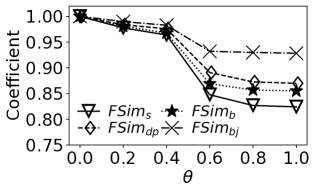
Varying $\theta$. For this analysis, we varied $\theta$ from 0 to 1 in steps of 0.2, and calculated the Pearson’s coefficient against the baseline case of $\theta=0$ (with $w^{+}$ and $w^{-}$ set to 0.4). The results in Figure 4(a) clearly show that the coefficients decrease as $\theta$ increases. This is reasonable as node pairs with $\mathcal{L}(\cdot)<\theta$ will not be considered by the mapping operator. Also, more node pairs are pruned as $\theta$ grows. However, the coefficients are still very high ($>0.8$) for all variants, even when $\theta=1$, which indicates that ${\mathsf{FSim}}_{\chi}$ is not sensitive to $\theta$.

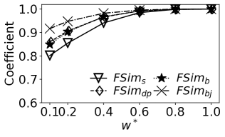
Varying $w^{*}$. To examine the influence of the weighting parameters, we varied $w^{*}$ from 0.1 to 1, where $w^{*}=1-w^{+}-w^{-}$. Recall that $\theta=1$ constrains mapping only the same-label nodes (Remark 2). As $w^{*}$ is label-relevant, we computed the coefficients of ${\mathsf{FSim}}_{\chi}$ (vs. ${\mathsf{FSim}}_{\chi}\{\theta=1\}$) by varying $w^{*}$. The results, reported in Figure 4, show that the coefficients increase as $w^{*}$ increases and at $w^{*}>0.6$, the coefficient is already almost 1. This is expected because a larger $w^{*}$ mitigates the impact of the label-constrained mapping. At a more reasonable setting of $w^{*}=0.2$, the coefficients sit at around 0.85, which indicates that ${\mathsf{FSim}}_{\chi}\{\theta=1\}$ aligns with ${\mathsf{FSim}}_{\chi}$ well. Hence, we set $w^{*}=0.2$ by default in subsequent tests.

(a) varying $\theta$

(b) varying $w^{*}$

Figure 4: Pearson’s correlation coefficients when varying $\theta$ and $w^{*}$

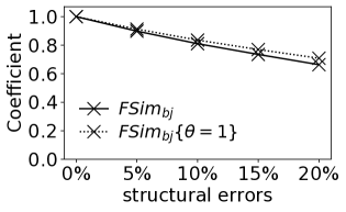
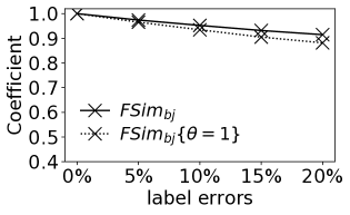
Robustness against Data Errors. Figure 5 plots the robustness of ${\mathsf{FSim}}_{{\mathsf{bj}}}$ against data errors, i.e., structural errors (with edges added/removed) and label errors (with certain labels missing), from one extreme ($\theta=0$) to the other ($\theta=1$) as an example of how all simulation variants performed. It is expected that the coefficients decrease as the error level increases. Yet, the coefficients remained high even at the 20% error level ($>0.7$ for both cases). This shows that ${\mathsf{FSim}}_{\chi}$ is robust to data errors, which conforms with one of the reasons why we initially thought to propose fractional simulation.

(a) varying structural errors

(b) varying label errors

Figure 5: Pearson’s correlation coefficients when varying the ratio of data errors

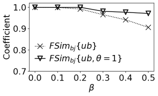
Sensitivity of Upper-bound Updating. To assess the influence of upper-bound updating (Section 3.4), we varied $\alpha$ (the approximate ratio) from 0 to 0.5 and $\beta$ (the threshold) from 0 to 1 in steps of $0.1$. Again, the results for all simulation variants were similar, so only the results for ${\mathsf{FSim}}_{{\mathsf{bj}}}\{{\mathsf{ub}}\}$ (vs. ${\mathsf{FSim}}_{{\mathsf{bj}}}$) and $\!{\mathsf{FSim}}_{\mathsf{bj}}\{{\mathsf{ub}},\theta=1\!\}$ (vs. ${\mathsf{FSim}}_{\mathsf{bj}}\{\theta=1\}$) are shown.

Varying $\beta$. Figure 6(a) shows the coefficients while varying $\beta$ from 0 to 0.5 with $\alpha$ fixed to 0.2. It is clear that the coefficients decrease as $\beta$ increases. This is reasonable as more node pairs are pruned, and the scores become less precise as $\beta$ gets larger. Note that when $\beta\geq 0.3$, the decreasing trend becomes smoother for ${\mathsf{FSim}}_{{\mathsf{bj}}}\{{\mathsf{ub}},\theta=1\}$. Observe that even at $\beta=0.5$, the coefficients are still very high ($>0.9$), which indicates that the validity of upper-bound updating is not sensitive to $\beta$. We thus set $\beta=0.5$ going forward to utilize as much pruning power as possible.

(a) varying $\beta$

(b) varying $\alpha$

Figure 6: Pearson’s correlation coefficients when varying $\alpha$ and $\beta$

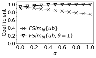
Varying $\alpha$. Figure 6(b) shows the coefficients when varying $\alpha$ from 0.0 to 1.0. We made two observations here. First, the coefficients of ${\mathsf{FSim}}_{\mathsf{bj}}\{{\mathsf{ub}}\}$ initially increase, then decrease as $\alpha$ gets larger. A possible reason is that $\alpha=0$ and $\alpha=1$ are at each extreme of the setting range, but the most appropriate setting lies somewhere in between. Second, the coefficients for ${\mathsf{FSim}}_{\mathsf{bj}}\{{\mathsf{ub}},\theta=1\}$ increase as $\alpha$ increases. Potentially, the true scores of pruned node pairs are larger than $1-w^{+}-w^{-}$, and thus a larger $\alpha$ is preferred. Note that when $\alpha=0$, i.e., when ignoring the pruned node pairs, the coefficients for both ${\mathsf{FSim}}_{\mathsf{bj}}\{{\mathsf{ub}}\}$ and ${\mathsf{FSim}}_{\mathsf{bj}}\{{\mathsf{ub}},\theta=1\}$ were above 0.9; hence, $\alpha=0$ became our default.

5.3 Efficiency

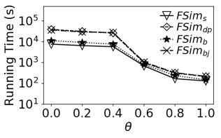
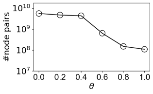
Varying $\theta$. With NELL as a representative of all tests, Figure 7(a) shows the running time of ${\mathsf{FSim}}_{\chi}$ while varying $\theta$ from 0 to 1. The experimental results show that ${\mathsf{FSim}}_{\chi}$ runs faster as $\theta$ increases, which is expected since a larger $\theta$ contributes to less candidate pairs to compute, as shown in Figure 7(b). We then compared the running time of different simulation variants under certain $\theta$ value. It is not surprising that ${\mathsf{FSim}}_{\mathsf{dp}}$ and ${\mathsf{FSim}}_{\mathsf{bj}}$ ran slower than the other two variants, as they contain a costly maximum-matching operation (cost analysis in Section 4). ${\mathsf{FSim}}_{\mathsf{b}}$ ran slower than ${\mathsf{FSim}}_{\mathsf{s}}$ because the mapping operator of ${\mathsf{FSim}}_{\mathsf{b}}$ considers both neighbors of a node pair(Table 3). At $\theta\geq 0.6$, the difference in running time for all variants was already very small. Considering the sensitivity analysis in Figure 4(a) as well as these results, $\theta=1$ seems a reasonable setting that renders both good coefficients and performance.

(a) running time

(b) number of node pairs

Figure 7: Running time of ${\mathsf{FSim}}_{\chi}$, $\chi\in\{{\mathsf{s}},{\mathsf{b}},{\mathsf{dp}},{\mathsf{bj}}\}$, while varying $\theta$

Varying the Datasets. Figure 8 reports the running time of ${\mathsf{FSim}}_{{\mathsf{bj}}}$, the most costly simulation variant, with different optimizations on all datasets. Additionally, experiments that resulted in out-of-memory errors have been omitted. From these tests, we made the observations: (1) the upper-bound updating alone contributed about 5$\times$ the performance gain compared to ${\mathsf{FSim}}_{{\mathsf{bj}}}\{{\mathsf{ub}}\}$ with ${\mathsf{FSim}}_{{\mathsf{bj}}}$. (2) Label-constrained mapping is the most effective optimization, making $\!{\mathsf{FSim}}_{{\mathsf{bj}}}\{\theta=1\}\!$ faster than $\!{\mathsf{FSim}}_{{\mathsf{bj}}}\!$ by up to 3 orders of magnitude. Applying both label-constrained mapping and upper-bound updating, ${\mathsf{FSim}}_{{\mathsf{bj}}}\{{\mathsf{ub}},\theta=1\}$ was the only algorithm that could complete the executions on all datasets in time, including the two largest ones, Amazon and ACMCit.

Figure 8: Running time of ${\mathsf{FSim}}_{{\mathsf{bj}}}$ on all datasets with different optimizations

Parallelization and Scalability. We studied the scalability of ${\mathsf{FSim}}_{\chi}$ with parallelization on two representative datasets, i.e., NELL and ACMCit (with more than 1 million nodes). The results for ${\mathsf{FSim}}_{{\mathsf{bj}}}\{{\mathsf{ub}},\theta=1\}$ follow.

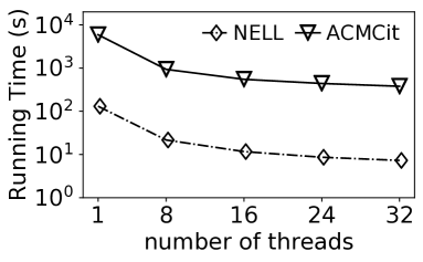
Varying the Number of Threads. Figure 9(a) shows the running time of ${\mathsf{FSim}}_{{\mathsf{bj}}}\{{\mathsf{ub}},\theta=1\}$ by varying the number of threads from 1 to 32. We observe that both curves demonstrate reasonable decreasing trends as the number of threads increases. The benefits from 1 to 8 threads are substantial. After 8, the reward ratio flattens due to the cost of thread scheduling. Specifically, when setting $t=32$, parallelization can speed up the computation by 15 to 17 times of magnitude.

(a) varying the number of threads

(b) varying density

Figure 9: Parallelization and Scalability

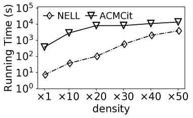
Varying Density. Figure 9(b) reports the running time of ${\mathsf{FSim}}_{{\mathsf{bj}}}\{{\mathsf{ub}},\theta=1\}$ (with 32 threads) while varying the density of the datasets from $\times 10$ to $\times 50$ by randomly adding edges. Unsurprisingly, the running times of both grew longer as the graphs became denser. However, although increased density means greater computational complexity in theory, it also means each node has more neighbors by expectation. Hence, the upper bound in Equation 6 may become smaller, which, in turn, contributes to greater upper-bound pruning power. This may offset some of the increase in computation complexity. Note that ${\mathsf{FSim}}_{\chi}$ finished within reasonable time on the ACMCit with $50\times$ more edges, indicating that it is scalable to the graphs with hundreds of millions of edges.

5.4 Case Studies

In this subsection, we used three case studies to exhibit the potential of ${\mathsf{FSim}}_{\chi}$ in the applications of pattern matching, node similarity measurement and RDF graph alignment. We will demonstrate the following strengths of our framework.

1. Our ${\mathsf{FSim}}_{\chi}$ framework quantifies the degree of simulation, which remedies the coarse “yes-or-no” semantics of simulation, significantly improves the effectiveness, and expand the scope of applying simulation.

2. When multiple simulation variants are suitable for a certain application, the ${\mathsf{FSim}}_{\chi}$ framework provides a flexible way to experiment with all suitable variants, so as to determine the one that performs the best.

Before simply driving into the case studies, the first question to answer is: which simulation variant should be used for a given application? We discuss the answer intuitively. Subgraph pattern matching is essentially asymmetric (matching the pattern graph to the data graph but not the other way around), and thus ${\mathsf{FSim}}_{{\mathsf{s}}}$ and ${\mathsf{FSim}}_{{\mathsf{dp}}}$ are appropriate choices. Node similarity measurement and graph alignment require symmetry, and hence ${\mathsf{FSim}}_{{\mathsf{b}}}$ and ${\mathsf{FSim}}_{{\mathsf{bj}}}$ are applied. The codes of all the baselines were provided by the respective authors. $\mathcal{L}(\cdot)$ was used indicator function since the semantics of node labels in the studied data were clear and without ambiguity.

Pattern Matching. In this case study, we first considered strong simulation (exact simulation by nature, [1]) and ${\mathsf{dp}}$-simulation [4] as two baselines, and compared them with ${\mathsf{FSim}}_{{\mathsf{s}}}$ and ${\mathsf{FSim}}_{{\mathsf{dp}}}$ to illustrate how ${\mathsf{FSim}}_{\chi}$ facilitates pattern matching. Figure 10 shows two example matches on the Amazon graph (see Table 4 for graph statistics). When answering query $Q_{1}$, strong simulation (and ${\mathsf{dp}}$-simulation) returns $G_{1}$, pictured in Figure 10(b), which is also the top-1 result of ${\mathsf{FSim}}_{\mathsf{s}}$ (and ${\mathsf{FSim}}_{{\mathsf{dp}}}$). Clearly, a simulation relation exists between $Q_{1}$ and $G_{1}$, and ${\mathsf{FSim}}_{\chi}$ captures $G_{1}$ with the highest score because of simulation definiteness (Definition 4). $Q_{2}$ adds two extra nodes with new labels to $Q_{1}$ but, with this modification, both strong simulation and ${\mathsf{dp}}$-simulation fail to return a result while ${\mathsf{FSim}}_{\chi}$ returns $G_{2}$ (strength S1), which closely matches $Q_{2}$ by missing only an edge.

(a) $Q_{1}$

(b) $G_{1}$

(c) $Q_{2}$

(d) $G_{2}$

Figure 10: Real-life matches on the Amazon graph. $G_{1}$ and $G_{2}$ are top-1 matches of ${\mathsf{FSim}}_{\chi}$ for answering queries $Q_{1}$ and $Q_{2}$ respectively. Nodes in match $G$ are marked by their item ids, while nodes in query $Q$ are marked by their labels. Nodes with the same shape have the same label.

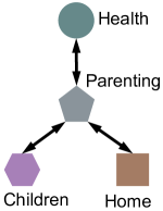
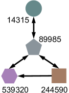
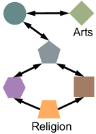
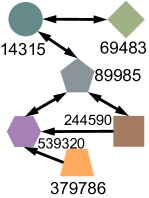
For a more complete study, we also compared the results of ${\mathsf{FSim}}_{\chi}$ with some other approximate pattern matching algorithms. The related algorithms can be summarized in two categories: (1) the edit-distance based algorithms, e.g., $\mathsf{SAPPER}$ [30] and $\mathsf{TSpan}$ [31], which enumerate all matches with mismatched edges up to a given threshold; and (2) the similarity-based algorithms that compute matches based on (sub)graph similarity or node similarity. To name a few, G-Ray [32] computes the “goodness” of a match based on node proximity. $\mathsf{IsoRank}$ [33], $\mathsf{NeMa}$ [34] and $\mathsf{NAGA}$ [35] find matches based on node similarity. $\mathsf{G}$-$\mathsf{Finder}$ [36] and $\mathsf{SAGA}$ [37] design cost functions with multiple components to allow node mismatches and graph structural differences. $\mathsf{SLQ}$ [38] and $S^{4}$ [39] find matches in RDF knowledge graphs by considering the semantics of queries. More specifically, $S^{4}$ uses the semantic graph edit distance to integrate structure similarity and semantic similarity. Note that, in the Amazon graph, an edge from $u$ to $v$ indicates that people are highly likely to buy item $v$ after buying item $u$ [1], and hence there is no complex semantics among edges. As a result, we choose $\mathsf{TSpan}$, $\mathsf{NAGA}$ and $\mathsf{G}$-$\mathsf{Finder}$, the state-of-the-art algorithms in each category, as another three baselines.

We followed the state-of-the-art algorithm $\mathsf{NAGA}$ [35] for match generation and quality evaluation. Briefly, node pairs with high ${\mathsf{FSim}}_{\chi}$ scores are considered to be “seeds”, and matches are generated by expanding the regions around the “seeds” subsequently. The evaluated queries are generated randomly by extracting subgraphs from the data graph and introducing structural noises (randomly insert edges, up to 33%) or label noises (randomly modify node labels, up to 33%). We then evaluated different algorithms across four query scenarios: (1) queries with no noises ($\mathsf{Exact}$); (2) queries with structural noises only ($\mathsf{Noisy}$-$\mathsf{E}$); (3) queries with label noises only ($\mathsf{Noisy}$-$\mathsf{L}$); and (4) queries with both kinds of noises ($\mathsf{Combined}$). Note that the queries are extracted from the graphs, which naturally serve as the “ground truth”. Given a query $Q$ and a returned match $\phi$ (we use top-1 match in this case study), the $F_{1}$ score is calculated by $F_{1}=\frac{2\cdot P\cdot R}{(P+R)}$, where $P=\frac{|\phi_{t}|}{|\phi|}$, $R=\frac{|\phi_{t}|}{|Q|}$, $\phi_{t}$ is a subset of $\phi$ that includes the correctly discovered node matches in $\phi$, and $|X|$ indicates the number of nodes in the match or graph, $\forall X\in\{\phi_{t},\phi,Q\}$.

Table 6: Average F1 scores (%) while answering queries in different scenarios on the Amazon dataset. $\mathsf{TSpan}$-x indicates miss-matching up to $x$ edges in $\mathsf{TSpan}$.

Query Scenario	Baselines					${\mathsf{FSim}}_{\chi}$
	$\mathsf{NAGA}$	$\mathsf{G}$-$\mathsf{Finder}$	$\mathsf{TSpan}$-1	$\mathsf{TSpan}$-3	Strong Simulation	${\mathsf{FSim}}_{{\mathsf{s}}}$	${\mathsf{FSim}}_{{\mathsf{dp}}}$
$\mathsf{Exact}$	30.2	100	100	100	100	100	100
$\mathsf{Noisy}$-$\mathsf{E}$	30.5	49.2	71.0	95.8	50.0	84.0	65.7
$\mathsf{Noisy}$-$\mathsf{L}$	20.6	40.7	-	-	33.3	75.1	73.2
$\mathsf{Combined}$	21.2	40.9	-	-	29.2	76.6	66.7

Table 6 shows the F1 scores of different algorithms. The result is an average from 100 random queries of sizes ranging from 3 to 13. ${\mathsf{dp}}$-simulation was not compared as it is similar to strong simulation. As with the last results, strong simulation performed poorly against noise. In comparison, ${\mathsf{FSim}}_{\chi}$ was more robust and performed much better (strength S1). Additionally, ${\mathsf{FSim}}_{{\mathsf{s}}}$ outperformed $\mathsf{NAGA}$, $\mathsf{G}$-$\mathsf{Finder}$ and $\mathsf{TSpan}$-1 by a big margin on all query scenarios. $\mathsf{TSpan}$-3 performed well in “$\mathsf{Exact}$” and “$\mathsf{Noisy}$-$\mathsf{E}$” with its highest F1 score of 95.8% for “$\mathsf{Noisy}$-$\mathsf{E}$”. This is because $\mathsf{TSpan}$-3 finds all matches with up to 3 mismatched edges, which is not less than the number of noisy edges in most queries. However, $\mathsf{TSpan}$ favors the case with missing edges rather than nodes. Thus, it has no results for “$\mathsf{Noisy}$-$\mathsf{L}$” and “$\mathsf{Combined}$”. In summary, ${\mathsf{FSim}}_{\chi}$ is qualified for approximate pattern matching (strength S1). While both ${\mathsf{s}}$- and ${\mathsf{dp}}$-simulation can be configured for the application, ${\mathsf{FSim}}_{{\mathsf{s}}}$ is more robust to noises and performs better than ${\mathsf{FSim}}_{{\mathsf{dp}}}$ (strength S2).

Node Similarity Measurement. In this case study, we compared ${\mathsf{FSim}}_{\chi}$ to four state-of-the-art similarity measurement algorithms: $\mathsf{PCRW}$ [40], $\mathsf{PathSim}$ [41], $\mathsf{JoinSim}$ [42] and $\mathsf{nSimGram}$ [43]. Following [43, 41], we used the DBIS dataset, which contains 60,694 authors, 72,902 papers and 464 venues. In DBIS, the venues and papers are labeled as “V” and “P", respectively. The authors are labeled by their names.

We first computed the top-5 most similar venues to WWW using all algorithms. The results are shown in Table 7. Note that WWW₁, WWW₂ and WWW₃ all represent the WWW venue but with different node ids in DBIS, and thus they are naturally similar to WWW. Although all algorithms gave reasonable results, ${\mathsf{FSim}}_{\mathsf{bj}}$ was the only one to return WWW₁, WWW₂ and WWW₃ in the top-5 results. In addition, if we applied exact ${\mathsf{b}}$- and ${\mathsf{bj}}$-simulation to the task, other than “WWW” itself (“Yes”), all the other venues had the same score (“No”). This shows that ${\mathsf{FSim}}_{\chi}$ can be applied to the scenarios that require fine-grained evaluation, such as node similarity measurement (strength S1).

Table 7: The top-5 similar venues for “WWW” of different algorithms

Rank	$\mathsf{PCRW}$	$\mathsf{PathSim}$	$\mathsf{JoinSim}$	$\mathsf{nSimGram}$	${\mathsf{FSim}}_{{\mathsf{b}}}$	${\mathsf{FSim}}_{{\mathsf{bj}}}$
1	WWW	WWW	WWW	WWW	WWW	WWW
2	SIGIR	CIKM	WWW1	CIKM	CIKM	WWW1
3	ICDE	SIGKDD	CIKM	SIGIR	ICDE	CIKM
4	VLDB	WISE	WSDM	WWW1	VLDB	WWW2
5	Hypertext	ICDM	WWW2	SIGKDD	SIGIR	WWW3

Following [43, 41], we further computed the top-15 most similar venues to 15 subject venues (same as [43]) of each algorithm. For each subject venue, we labeled each returned venue with a relevance score: 0 for non-relevant, 1 for some-relevant, and 2 for very-relevant, considering both the research area and venue ranking in [44]. For example, the relevance score for ICDE and VLDB is 2 as both are top-tier conferences in the area of database. We then evaluated the ranking quality of the algorithms using nDCG (the larger the score, the better).

Table 8: NDCG results of node similarity algorithms

Baselines				Fractional $\chi$-simulation
$\mathsf{PCRW}$	$\mathsf{PathSim}$	$\mathsf{JoinSim}$	$\mathsf{nSimGram}$	${\mathsf{FSim}}_{{\mathsf{b}}}$	${\mathsf{FSim}}_{{\mathsf{bj}}}$
0.684	0.684	0.689	0.700	0.699	0.733

Table 8 shows the nDCG results. Accordingly, ${\mathsf{FSim}}_{\chi}$ outperforms the state-of-the-art algorithms by a large margin. This indicates that ${\mathsf{FSim}}_{\chi}$ is qualified to measure node similarity on labeled graphs (strength S1). The result that ${\mathsf{FSim}}_{\mathsf{bj}}$ outperforms ${\mathsf{FSim}}_{\mathsf{b}}$ in both the “WWW” case and the general evaluation suggests ${\mathsf{FSim}}_{\mathsf{bj}}$ is a better candidate for similarity measurement (strength S2).

RDF Graph Alignment. We investigate the potential of ${\mathsf{FSim}}_{\chi}\!$ in RDF graph alignment and briefly discuss its performance below. We followed Olap [7] (a bisimulation-based alignment algorithm) to align three different versions of biological graphs from different times, $G_{1}$, $G_{2}$ and $G_{3}$ [27]. $G_{1}$ has 133,195 nodes and 273,512 edges, $G_{2}$ has 138,651 nodes and 285,000 edges, $G_{3}$ includes 144,879 nodes and 298,564 edges, and all of them have 8 node labels and 23 edge labels. Note that the original URI values in these datasets do not change over time. Hence, we can use this information to identify the ground truth alignment. In addition to Olap, we also included another four state-of-the-art algorithms, namely $k$-bisimulation [10], gsaNA [45], $\mathsf{FINAL}$ [46] and $\mathsf{EWS}$ [47]. When aligning graphs with ${\mathsf{FSim}}_{\chi}$, a node $u\in V_{1}$ will be aligned to a node set $A_{u}=\mathop{\mathrm{argmax}}_{v\in V_{2}}{\mathsf{FSim}}_{\chi}(u,v)$, while with $k$-bisimulation, $u$ will be aligned to $A_{u}=\{v|v\in V_{2}\wedge u\text{ and }v\text{ are bisimilar}\}$. The F1 score of ${\mathsf{FSim}}_{\chi}$ and $k$-bisimulation is calculated by $F1=\sum_{u\in V_{1}}\frac{2\cdot P_{u}\cdot R_{u}}{|V_{1}|(P_{u}+R_{u})}$, where $P_{u}$ (resp. $R_{u}$) is $\frac{1}{|A_{u}|}$ (resp. 1) if $A_{u}$ contains the ground truth, and 0 otherwise. We follow the settings in the related papers for the other baselines.

Table 9 reports the F1 scores of each algorithm. Note that we also tested the bisimulation, which resulted in 0% F1 scores in both cases since there is no exact bisimulation relation between two graphs. $k$-bisimulation performs better than bisimulation as it, to some extent, approximates bisimulation. From Table 9, our ${\mathsf{FSim}}_{\chi}$ had the highest F1 scores and thus outperformed all the other baselines. This shows that we can apply ${\mathsf{FSim}}_{\mathsf{b}}$ and ${\mathsf{FSim}}_{\mathsf{bj}}$ with high potential for graph alignment (strength S1). ${\mathsf{FSim}}_{{\mathsf{b}}}$ outperforms ${\mathsf{FSim}}_{{\mathsf{bj}}}$ and thus is a better candidate for graph alignment (strength S2).

Table 9: The F1 scores (%) of each algorithm when aligning two graphs. $x$-bisim indicates setting $k=x$ in $k$-bisimulation.

Graphs	Baselines						${\mathsf{FSim}}_{\chi}$
	$2$-bisim	$4$-bisim	Olap	gsaNA	$\mathsf{FINAL}$	$\mathsf{EWS}$	${\mathsf{FSim}}_{{\mathsf{b}}}$	${\mathsf{FSim}}_{{\mathsf{bj}}}$
$G_{1}$-$G_{2}$	19.9	9.1	37.9	11.8	55.2	70.8	97.6	96.5
$G_{1}$-$G_{3}$	53.0	10.9	37.6	14.9	52.7	65.3	96.9	95.6

Efficiency Evaluation. Given the superior effectiveness of ${\mathsf{FSim}}_{\chi}$ in the above case studies, one may also be interested in its efficiency. Next, we show the running time of ${\mathsf{FSim}}_{\chi}$ (with 32 threads) and the most effective baseline in each case study. We will also report the running time of exact simulation (or its variant) if it is applied and effective in the case study. For pattern matching, ${\mathsf{FSim}}_{\chi}$ on average took 0.25s for each query. In comparison, exact simulation took around 1.2s, and $\mathsf{TSpan}$, the most effective baseline, spent more than 70s. In similarity measurement, $\mathsf{nSimGram}$ took 0.03ms to compute a single node pair, while ${\mathsf{FSim}}_{\chi}$ finished the computation within 6500s for 134060$\times$134060 pairs or roughly 0.0004ms per pair. In graph alignment, $k$-bisimulation ($k=4$) spent 0.4s for the computation, and $\mathsf{EWS}$ spent 1496s. Our ${\mathsf{FSim}}_{\chi}$ ran a bit slower than $\mathsf{EWS}$ and took 3120s, which is tolerable as it is much more effective than the other algorithms. Note that it is not straightforward and potentially unfair to compare with all the baselines as they either focus on per-query computation (e.g., $\mathsf{PathSim}$ and $\mathsf{JoinSim}$) or have been individually implemented in different languages (e.g., Olap in Python and $\mathsf{FINAL}$ in Matlab).

6 Related Work

Simulation and Its Variants. In this paper, we focused on four simulation variants: simple simulation [2, 1], bisimulation [3], degree-preserving simulation [4] and bijective simulation. The original definition of simulation [2] only considered out-neighbors, but Ma et al.’s redefinition in 2011 [1] takes in-neighbors into account and hence is the definition we used. Reverting to the original definition is as easy as setting $w^{-}=0$ in our framework. Additionally, we discussed a variant of approximate bisimulation, namely $k$-bisimulation [20, 21, 22, 10], and investigated its relation to our framework (Section 4.3). There are other variants that have not yet included in the framework, including bounded simulation [5] and weak simulation [3]. These variants consider the $k$-hop neighbors ($k\geq 1$) in addition to the immediate neighbors. As an interesting future work, we will study to incorporate them in our framework. There are also some algorithms that aim to compute simulation (variants) efficiently and effectively, e.g., a hash-based algorithm in [10], external-memory algorithms in [8, 22], a distributed algorithm in [21] and a partition refinement algorithm in [48]. However, all these algorithms compute the “yes-or-no” simulation (or its variant) and cannot provide fractional scores as proposed in this paper.

Node Similarity Measures. We have shown that ${\mathsf{FSim}}_{{\mathsf{bj}}}$ is qualified for node similarity measurement. Thus, we review node similarity measures on labeled graphs. $\mathsf{SimRank}$ [18] and $\mathsf{RoleSim}$ [19] are two representative measures, and their relations to our ${\mathsf{FSim}}_{\chi}$ have been discussed in Section 4.3. As these two measures are less effective in computing node similarity on labeled graphs [43, 41], similarity measures [43, 49, 41, 42] were proposed. $\mathsf{PathSim}$ [41], for instance, uses a ratio of meta-paths connecting two nodes as the measure. $\mathsf{JoinSim}$ [42] is similar to $\mathsf{PathSim}$, but it satisfies the triangle inequality. $\mathsf{nSimGram}$ [43] computes node similarity based on q-grams instead of meta-paths to capture more topology information. Note that these measures cannot substitute our work as their scores are not related to simulation and thus are not suitable to quantify the extent of simulation.

Similarity-based Applications. There are a number of works on pattern matching and graph alignment that are based on node similarity techniques. These works may differ in measuring node similarities. Specifically, $\mathsf{IsoRank}$ [33] computes the similarity between two nodes based on an weighted average of their neighbors’ scores. $\mathsf{NeMa}$ [34] defines a vector that encodes the neighborhood information for each node. The distance between two nodes is then computed from these vectors. $\mathsf{NAGA}$ [35] leverages statistical significance through chi-square measure to compute node similarity. $\mathsf{REGAL}$ [50] measures the similarity of two nodes by taking the information of $k$-hop neighbors into account. $\mathsf{FIRST}$ [51] and $\mathsf{FINAL}$ [46] use a Sylvester equation to compute similarities, which encodes structural consistency and attribute consistency of two networks. For similar reasons, these works are also not suitable to quantify the degree of simulation.

7 Conclusion

In this paper, we formally define fractional $\chi$-simulation to quantify the degree to which one node simulates another by a $\chi$-simulation. We then propose the ${\mathsf{FSim}}_{\chi}$ computation framework to realize the quantification for all $\chi$-simulations. We conduct extensive experiments to demonstrate the effectiveness and efficiency of the fractional $\chi$-simulation framework. Considering end-users are also interested in the top-k similarity search. In the future, we plan to devise efficient techniques to process top-k queries based on the ${\mathsf{FSim}}_{\chi}$.

References

- [1] Shuai Ma, Yang Cao, Wenfei Fan, Jinpeng Huai, and Tianyu Wo. Capturing topology in graph pattern matching. PVLDB, 5(4):310–321, 2011.
- [2] Robin Milner. An algebraic definition of simulation between programs. In IJCAI, pages 481–489, 1971.
- [3] Robin Milner. Communication and concurrency. 1989.
- [4] Chunyao Song, Tingjian Ge, Cindy X. Chen, and Jie Wang. Event pattern matching over graph streams. PVLDB, 8(4):413–424, 2014.
- [5] Wenfei Fan, Jianzhong Li, Shuai Ma, Nan Tang, Yinghui Wu, and Yunpeng Wu. Graph pattern matc-hing: From intractable to polynomial time. PVLDB, 3(1):264–275, 2010.
- [6] Shuai Ma, Yang Cao, Wenfei Fan, Jinpeng Huai, and Tianyu Wo. Strong simulation: Capturing topology in graph pattern matching. TODS, 39(1):4:1–4:46, 2014.
- [7] Peter Buneman and Slawek Staworko. RDF graph alignment with bisimulation. PVLDB, 9(12):1149–1160, 2016.
- [8] Jelle Hellings, George H. L. Fletcher, and Herman J. Haverkort. Efficient external-memory bisimulation on dags. In SIGMOD, pages 553–564, 2012.
- [9] Alexander Schätzle, Antony Neu, Georg Lausen, and Martin Przyjaciel-Zablocki. Large-scale bisimulation of RDF graphs. In SWIM@SIGMOD, 2013.
- [10] Wouter van Heeswijk, George H. L. Fletcher, and Mykola Pechenizkiy. On structure preserving sampling and approximate partitioning of graphs. In ACM Symposium on Applied Computing, pages 875–882, 2016.
- [11] Prakash Ramanan. Covering indexes for XML queries: Bisimulation - simulation = negation. In VLDB, pages 165–176, 2003.
- [12] Wenfei Fan, Jianzhong Li, Xin Wang, and Yinghui Wu. Query preserving graph compression. In SIGMOD, pages 157–168, 2012.
- [13] George H. L. Fletcher, Dirk Van Gucht, Yuqing Wu, Marc Gyssens, Sofia Brenes, and Jan Paredaens. A methodology for coupling fragments of xpath with structural indexes for XML documents. Inf. Syst., 34(7):657–670, 2009.
- [14] Raghav Kaushik, Philip Bohannon, Jeffrey F. Naughton, and Henry F. Korth. Covering indexes for branching path queries. In SIGMOD, pages 133–144, 2002.
- [15] Yuya Sasaki, George Fletcher, and Makoto Onizuka. Structural indexing for conjunctive path queries. CoRR, 2020.
- [16] Solo: https://en.wikipedia.org/wiki/Solo:_A_Star_Wars_Story.
- [17] Nino Shervashidze, Pascal Schweitzer, Erik Jan van Leeuwen, Kurt Mehlhorn, and Karsten M. Borgwardt. Weisfeiler-lehman graph kernels. JMLR, 2011.
- [18] Glen Jeh and Jennifer Widom. Simrank: a measure of structural-context similarity. In SIGKDD, pages 538–543, 2002.
- [19] Ruoming Jin, Victor E. Lee, and Hui Hong. Axiomatic ranking of network role similarity. In SIGKDD, pages 922–930, 2011.
- [20] Luca Aceto, Anna Ingólfsdóttir, and Jirí Srba. The algorithmics of bisimilarity. In Advanced Topics in Bisimulation and Coinduction. 2012.
- [21] Yongming Luo, Yannick de Lange, George H. L. Fletcher, Paul De Bra, Jan Hidders, and Yuqing Wu. Bisimulation reduction of big graphs on mapreduce. In BNCOD, 2013.
- [22] Yongming Luo, George H. L. Fletcher, Jan Hidders, Yuqing Wu, and Paul De Bra. External memory k-bisimulation reduction of big graphs. In CIKM, 2013.
- [23] David Avis. A survey of heuristics for the weighted matching problem. Networks, 13(4):475–493, 1983.
- [24] László Babai. Graph isomorphism in quasipolynomial time. In ACM Symposium on Theory of Computing, pages 684–697, 2016.
- [25] KONECT: http://konect.uni-koblenz.de/.
- [26] NELL: https://github.com/xwhan/DeepPath.
- [27] The guide to pharmacology: https://www.guidetopharmacology.org.
- [28] SNAP: http://snap.stanford.edu/data.
- [29] ArnetMiner: https://www.aminer.org/data.
- [30] Shijie Zhang, Jiong Yang, and Wei Jin. SAPPER: subgraph indexing and approximate matching in large graphs. PVLDB, 3(1):1185–1194, 2010.
- [31] Gaoping Zhu, Xuemin Lin, Ke Zhu, Wenjie Zhang, and Jeffrey Xu Yu. Treespan: efficiently computing similarity all-matching. In SIGMOD, pages 529–540, 2012.
- [32] Hanghang Tong, Christos Faloutsos, Brian Gallagher, and Tina Eliassi-Rad. Fast best-effort pattern matching in large attributed graphs. In SIGKDD, 2007.
- [33] Rohit Singh, Jinbo Xu, and Bonnie Berger. Global alignment of multiple protein interaction networks with application to functional orthology detection. Proc. Natl. Acad. Sci., 105(35):12763–12768, 2008.
- [34] Arijit Khan, Yinghui Wu, Charu C. Aggarwal, and Xifeng Yan. Nema: Fast graph search with label similarity. PVLDB, 6(3):181–192, 2013.
- [35] Sourav Dutta, Pratik Nayek, and Arnab Bhattacharya. Neighbor-aware search for approximate labeled graph matching using the chi-square statistics. In WWW, pages 1281–1290, 2017.
- [36] Lihui Liu, Boxin Du, Jiejun Xu, and Hanghang Tong. G-finder: Approximate attributed subgraph matching. In IEEE Big Data, pages 513–522, 2019.
- [37] Yuanyuan Tian, Richard C. McEachin, Carlos Santos, David J. States, and Jignesh M. Patel. SAGA: a subgraph matching tool for biological graphs. Bioinform., 2007.
- [38] Shengqi Yang, Yinghui Wu, Huan Sun, and Xifeng Yan. Schemaless and structureless graph querying. PVLDB, 7(7):565–576, 2014.
- [39] Weiguo Zheng, Lei Zou, Wei Peng, Xifeng Yan, Shaoxu Song, and Dongyan Zhao. Semantic SPARQL similarity search over RDF knowledge graphs. PVLDB, 2016.
- [40] Ni Lao and William W. Cohen. Relational retrieval using a combination of path-constrained random walks. Machine Learning, 81(1):53–67, 2010.
- [41] Yizhou Sun, Jiawei Han, Xifeng Yan, Philip S. Yu, and Tianyi Wu. Pathsim: Meta path-based top-k similarity search in heterogeneous information networks. PVLDB, 4(11):992–1003, 2011.
- [42] Yun Xiong, Yangyong Zhu, and Philip S. Yu. Top-k similarity join in heterogeneous information networks. TKDE, 27(6):1710–1723, 2015.
- [43] Alessio Conte, Gaspare Ferraro, Roberto Grossi, Andrea Marino, Kunihiko Sadakane, and Takeaki Uno. Node similarity with q-grams for real-world labeled networks. In SIGKDD, pages 1282–1291, 2018.
- [44] Core rankings portal: http://portal.core.edu.au/conf-ranks/.
- [45] Abdurrahman Yasar and Ümit V. Çatalyürek. An iterative global structure-assisted labeled network aligner. In SIGKDD, pages 2614–2623, 2018.
- [46] Si Zhang and Hanghang Tong. FINAL: fast attributed network alignment. In SIGKDD, pages 1345–1354, 2016.
- [47] Ehsan Kazemi, Seyed Hamed Hassani, and Matthias Grossglauser. Growing a graph matching from a handful of seeds. PVLDB, 8(10):1010–1021, 2015.
- [48] Francesco Ranzato. An efficient simulation algorithm on kripke structures. Acta Informatica, 51(2):107–125, 2014.
- [49] Zhipeng Huang, Yudian Zheng, Reynold Cheng, Yizhou Sun, Nikos Mamoulis, and Xiang Li. Meta structure: Computing relevance in large heterogeneous information networks. In SIGKDD, pages 1595–1604, 2016.
- [50] Mark Heimann, Haoming Shen, Tara Safavi, and Danai Koutra. REGAL: representation learning-based graph alignment. In ACM CIKM, pages 117–126, 2018.
- [51] Boxin Du, Si Zhang, Nan Cao, and Hanghang Tong. FIRST: fast interactive attributed subgraph matching. In SIGKDD, pages 1447–1456, 2017.