Accelerated Algorithms for Convex and Non-Convex Optimization on Manifolds

Abstract

We propose a general scheme for solving convex and non-convex optimization problems on manifolds. The central idea is that, by adding a multiple of the squared retraction distance to the objective function in question, we “convexify” the objective function and solve a series of convex sub-problems in the optimization procedure. One of the key challenges for optimization on manifolds is the difficulty of verifying the complexity of the objective function, e.g., whether the objective function is convex or non-convex, and the degree of non-convexity. Our proposed algorithm adapts to the level of complexity in the objective function. We show that when the objective function is convex, the algorithm provably converges to the optimum and leads to accelerated convergence. When the objective function is non-convex, the algorithm will converge to a stationary point. Our proposed method unifies insights from Nesterov’s original idea for accelerating gradient descent algorithms with recent developments in optimization algorithms in Euclidean space. We demonstrate the utility of our algorithms on several manifold optimization tasks such as estimating intrinsic and extrinsic Fréchet means on spheres and low-rank matrix factorization with Grassmann manifolds applied to the Netflix rating data set.

1 Introduction

Optimization is a near ubiquitous tool used in a wide-range of disciplines including the physical sciences, applied mathematics, engineering and the social sciences. Formally, it aims to maximize or minimize some quantitative criteria, namely, the objective function with respect to some parameters of interest. In many broad, complex learning in modern data science, the parameters are naturally defined over to be on a manifold. The emerging field of statistics on manifolds based on Fréchet means (Bhattacharya and Bhattacharya,, 2012; Bhattacharya and Lin,, 2017) can be viewed as one of the notable examples of optimization on general manifolds.

Another example can be found in building scalable recommender systems where extracting a low-rank matrix involves an optimization problem over a Grassmann manifold (Boumal et al.,, 2019). Recent development in geometric deep learning, where the input or output layer constrained to be on a Riemannian manifold (Lohit and Turaga,, 2017; Huang and Gool,, 2017; Huang et al.,, 2017), constitutes another important class of applications. Other applications arise in diverse areas ranging from medical imaging analysis, Procrustes shape matching, dimension reduction, dynamic subspace tracking, and cases involving ranking and orthogonality constraints–among many others. This proliferation of manifold-valued applications demands fundamental development of models, algorithms and theory for solving optimization problems over non-Euclidean spaces.

The current literature on optimization over manifolds mainly focuses on extending existing Euclidean space algorithms, such as Newton’s method (Smith,, 2014; Ring and Wirth,, 2012), conjugate gradient descent (Edelman et al.,, 1998; Nishimori et al.,, 2008), steepest descent (Absil et al.,, 2010), trust-region methods (Absil et al.,, 2007; Boumal and Absil,, 2011) and others. Many of the objective functions in manifold optimization problems are very complex. One of key challenges for solving such problems lies in the difficulty in verifying the convexity and the degree of convexity of the objective function. Current approaches cannot adapt to the complexity of the problem at hand in manifold spaces.

We take a major step to address these issues by proposing a general scheme to solve convex and non-convex optimization problems on manifolds using gradient-based algorithms originally designed for convex functions. The key idea is to “convexify” the objective function by adding a multiple of the squared retraction distance. The proposed algorithm does not require knowledge of whether the objective function is convex but will automatically converges to an optima if the function is strongly convex. When the objective is non-convex, it achieves rapid convergence to a stationary point. The proposed algorithm is a generalization of Nesterov acceleration (Nesterov,, 2004), which improves the convergence rate of gradient descent algorithms. Our algorithm (which we call $\mathcal{A}_{2}$) takes any general existing optimization method (which we call $\mathcal{A}$), originally designed for convex functions, and converts it into a method applicable for non-convex functions.

Similar schemes have been explored for optimization problems in Euclidean space (Paquette et al.,, 2018). Generalizations to arbitrary manifolds, however, require fundamentally novel theoretical development. In the Euclidean case, the gradient steps are taken towards lines, whereas for the manifold we use the retraction curves which crucially affects the result and raises the difficulty in proving convergence. Also for manifolds, it is not trivial to correctly convexify the ’weakly-convex function’, a broad class of non-convex functions on manifolds we consider which account for most of the interesting examples of non-convex functions in machine learning. We propose a novel idea to convexify the objective locally with the help of the retraction. Key features of our algorithm include adaptation to the unknown weak convexity of the objective function and automatic Nesterov acceleration. The proposed algorithm can be used to accelerate a broad class of $\mathcal{A}$ algorithms including gradient descent as well as parallel optimization approaches (see Saparbayeva et al.,, 2018).

Our paper is organized as follows: In Section 2, we introduce related work on accelerated optimization algorithms. Next, we present our proposed acceleration algorithm on manifolds in Section 3 and present theoretical convergence results. In Section 4, we consider a simulation study of estimating Fréchet means and a real data example using the Netflix prize data set in a matrix completion problem.

2 Related work

Liu et al., (2017) propose accelerated first-order methods for geodesically convex optimization on Riemannian manifolds. This is a direct generalization of Nesterov’s original linear extrapolation mechanism to general Riemannian manifolds via a non-linear operator. One drawback of Liu et al., (2017) is that the accelerated step of their algorithm involves exact solving of non-trivial implicit equations.

Zhang and Sra, 2018a later proposed a computationally tractable accelerated gradient algorithm and a novel estimation sequence for convergence analysis. Our approach is fundamentally different from theirs. We regularize an objective function with a squared retraction distance (see Proposition 1), solve a sequence of convex subproblems, adapt to the degree of weak convexity of the objective function, and produce accelerated rates for convex objectives. Even in the convex case, our approach can deal with a much broader class of retraction-based convex functions.

Paquette et al., (2018) proposes a general scheme called “Catalyst acceleration” for solving general optimizations in Euclidean space, which has inspired development of some ideas for our work. Similar ideas have been explored for convex functions in Euclidean space in both theory and practice (Lin et al.,, 2017). However, optimization problems on manifolds are of fundamentally different nature and require development of substantially new tools and theory.

There is an interesting line of work on proposing fast algorithms for stochastic optimization on manifolds (see Zhang et al.,, 2016, 2018; Zhou et al.,, 2019; Bonnabel,, 2013) which employ very different techniques such as minibatching, variance reduction and utilizing the uncertainty of inputs. Methods like Zhang and Sra, 2018b propose optimization methods that are analogous to Nesterov-type algorithms for manifold spaces.

3 Accelerated algorithms for optimization on manifolds

3.1 Weakly convex functions on manifolds with respect to retraction mapping

We first define general retraction-based, weakly convex, convex, and strongly convex functions by generalizing from their geodesic-based counterparts . We then prove an important proposition that can transform a non-convex function into a convex one simply by adding a multiple of the squared retraction-distance to the objective function.

Definition 1.

A retraction on a manifold $\mathcal{M}$ is a smooth mapping from its tangent bundle $\mathcal{R}:T\mathcal{M}\rightarrow\mathcal{M}$ with the following properties:

1. $\mathcal{R}_{\theta}(0_{\theta})=\mathcal{R}(\theta,0_{\theta})=\theta,$ where $0_{\theta}$ denotes the zero vector on the tangent space $T_{\theta}\mathcal{M};$

2. For any point $\theta\in\mathcal{R}$ the differential $d(\mathcal{R}_{\theta})$ of the retraction mapping at the zero vector $0_{\theta}\in T_{\theta}\mathcal{M}$ has to be equal to the identity mapping on $T_{\theta}\mathcal{M},$ that is $d(\mathcal{R}_{\theta}(0_{\theta}))=d\big{(}\mathcal{R}(\theta,0_{\theta})\big{)}={\rm id}_{T_{\theta}\mathcal{M}},$ where ${\rm id}_{T_{\theta}\mathcal{M}}$ denotes the identity mapping on $T_{\theta}\mathcal{M}.$

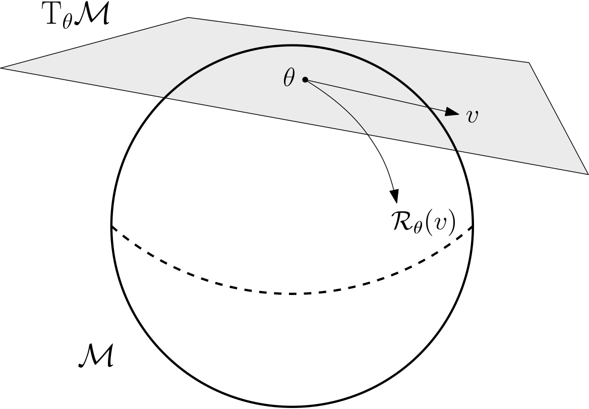
The exponential map on a Riemannian manifold can be viewed as a special case of the retraction map, and the inverse-exponential map is a special case of the inverse-retraction map. A good choice of retraction map can lead to substantial reduction in computation burden compared to the exponential map. We see an example in Section 4.2 on the choice of a retraction map for Grassmannian; Figure 1 provides a visualization of a retraction map.

Figure 1: Illustration of a retraction map on a manifold

We first define the retraction distance function on $\mathcal{M}$

$$d_{\mathcal{R}}(\theta_{0},\theta)=\|\mathcal{R}_{\theta_{0}}^{-1}\theta\|.$$

Since at zero the differential of the retraction map is the identity, there is a small enough neighborhood $D$ of the point $\theta$ where the inverse retraction map $\mathcal{R}_{\theta}^{-1}$ is bi-Lipschitz continuous in $D,$ i.e. $d_{\mathcal{R}}$ satisfies inequalities

$$\frac{1}{K_{1}}d_{\mathcal{R}}(\vartheta_{1},\vartheta_{2})\leq\|\mathcal{R}_{\theta}^{-1}\vartheta_{1}-\mathcal{R}_{\theta}^{-1}\vartheta_{2}\|\leq K_{2}d_{\mathcal{R}}(\vartheta_{1},\vartheta_{2}),$$

where $\vartheta_{1},\vartheta_{2}\in D,$ and $K_{1}\geq 1,$ and $K_{2}\geq 1.$

In addition, we also require the squared retraction distance function to be $2R_{1}$-strongly retraction convex around $\vartheta$–that is, for some $\delta>0$ and constant $0\leq R_{1}\leq 1$ the following inequality holds:

$$d_{\mathcal{R}}^{2}(\theta_{2},\vartheta)\geq d_{\mathcal{R}}^{2}(\theta_{1},\vartheta)+\langle\nabla d_{\mathcal{R}}^{2}(\theta_{1},\vartheta),\mathcal{R}_{\theta_{1}}^{-1}\theta_{2}\rangle+R_{1}d_{\mathcal{R}}^{2}(\theta_{1},\theta_{2}),$$ (1)

where $d_{\mathcal{R}}(\theta_{i},\vartheta)<\delta,$ $i=1,2.$ Due to the fact that at the zero vector $0_{\vartheta}\in T_{\vartheta}\mathcal{M}$ the differential of $\mathcal{R}_{\vartheta}$ is equal to identity mapping, we can see that in a small neighborhood of $\vartheta$, the square retraction distance function behaves like the square normal function which is strongly convex.

Definition 2.

Consider a function $f:\mathcal{M}\rightarrow\bar{\mathbb{R}}$ and a point $\theta$ with $f(\theta)$ finite. The $\mathcal{R}-$subdifferential of $f$ at $\theta$ is the set

$$\begin{split}\partial f(\theta)=\Big{\{}v\in T_{\theta}\mathcal{M}:f(\vartheta)\geq f(\theta)+\langle v,\mathcal{R}^{-1}_{\theta}\vartheta\rangle+o\big{(}d_{\mathcal{R}}(\theta,\vartheta)\big{)}\\ \forall\vartheta\in\mathcal{M}\Big{\}}.\end{split}$$

We now define the notion of convex functions on manifolds with respect to the retraction map.

Definition 3.

A function $f$ is convex with respect to the retraction $\mathcal{R}$ if for any points $\theta_{1},\theta_{2}\in\mathcal{M}$ the inequality holds

$$f(\theta_{2})\geq f(\theta_{1})+\langle v,\mathcal{R}_{\theta_{1}}^{-1}\theta_{2}\rangle,\qquad v\in\partial f(\theta_{1}).$$ (2)

Now we are ready to define one of the most important classes of non-convex functions called weakly-convex functions which constitute many interesting applications of non-convex functions in machine learning.

Definition 4.

A function $f$ is $\rho$-weakly convex with respect to the retraction $\mathcal{R}$ if for any points $\theta_{1},\theta_{2}\in\mathcal{M}$ the inequality holds

$$f(\theta_{2})\geq f(\theta_{1})+\langle v,\mathcal{R}_{\theta_{1}}^{-1}\theta_{2}\rangle-\frac{\rho}{2}d_{\mathcal{R}}^{2}(\theta_{1},\theta_{2}),\qquad v\in\partial f(\theta_{1}).$$ (3)

Given the strong retraction convexity of the squared retraction distance (see (1)), we can regularize the weakly convex function $f$ by adding the term $\frac{\kappa}{2}d_{\mathcal{R}}^{2}(\theta,\vartheta)$ and turn it into a convex function through the following proposition.

Proposition 1.

Let $d_{\mathcal{R}}$ be a retraction distance that is strong-retraction convex or satisfies the inequality (1) in the subset $D\subset\mathcal{M}.$ Then the function $f$ is $R_{1}\kappa$-weakly convex in $D$ if and only if the function

$$h_{\kappa}(\theta,\vartheta)=f(\theta)+\frac{\kappa}{2}d_{\mathcal{R}}^{2}(\theta,\vartheta)$$

is convex in $D.$

Proof.

Let $f$ be $\rho$-weakly convex. Then for any $\theta_{1},\theta_{2}\in D$ and any $\lambda\in[0,1]$

$$f(\theta_{2}) \geq f(\theta_{1})+\langle\partial f(\theta_{1}),\mathcal{R}_{\theta_{1}}^{-1}\theta_{2}\rangle-\frac{R_{1}\kappa}{2}d_{\mathcal{R}}^{2}(\theta_{1},\theta_{2})$$

$$\geq f(\theta_{1})+\langle\partial f(\theta_{1}),\mathcal{R}_{\theta_{1}}^{-1}\theta_{2}\rangle+\frac{\kappa}{2}d_{\mathcal{R}}^{2}(\theta_{1},\vartheta)$$

$$\quad\quad+\langle\nabla\frac{\kappa}{2}d_{\mathcal{R}}^{2}(\theta_{1},\vartheta),\mathcal{R}_{\theta_{1}}^{-1}\theta_{2}\rangle-\frac{\kappa}{2}d_{\mathcal{R}}^{2}(\theta_{2},\vartheta),$$

which implies

$$h_{\kappa}(\theta_{2},\vartheta)\geq h_{\kappa}(\theta_{1},\vartheta)+\langle\partial h_{\kappa}(\theta_{1},\vartheta),\mathcal{R}_{\theta_{1}}^{-1}\theta_{2}\rangle.$$

∎

For functions defined on an Euclidean space we have a definition of a weakly convex function that is equivalent to (3):

$$f\big{(}\mathcal{R}_{\vartheta}(\lambda\mathcal{R}^{-1}_{\vartheta}\theta)\big{)}\leq\lambda f(\theta)+(1-\lambda)f(\vartheta)+\frac{\rho\lambda(1-\lambda)}{2}d_{\mathcal{R}}^{2}(\theta,\vartheta).$$ (4)

Over the manifold, however, there is no such straightforward equivalence. This is due to the distance function $d_{\mathcal{R}}^{2}(\vartheta,\theta)$ which does not satisfy the following equality:

$$d_{\mathcal{R}}^{2}(\mathcal{R}_{\theta_{1}}\lambda\mathcal{R}_{\theta_{1}}^{-1}\theta_{2},\vartheta) =\lambda d_{\mathcal{R}}(\theta_{2},\vartheta)+(1-\lambda)d_{\mathcal{R}}^{2}(\theta_{1},\vartheta)$$

$$\quad\quad-\lambda(1-\lambda)d_{\mathcal{R}}^{2}(\theta_{1},\theta_{2}).$$ (5)

Nevertheless in some neighborhood of $\vartheta,$, for some $\delta>0$, the following inequality holds

$$\begin{split}d_{\mathcal{R}}^{2}(\mathcal{R}_{\theta_{1}}\lambda\mathcal{R}_{\theta_{1}}^{-1}\theta_{2},\vartheta)\leq\lambda d_{\mathcal{R}}^{2}(\theta_{2},\vartheta)+(1-\lambda)d_{\mathcal{R}}^{2}(\theta_{1},\vartheta)\\ -\lambda(1-\lambda)R_{1}d_{\mathcal{R}}^{2}(\theta_{1},\theta_{2}),\end{split}$$ (6)

where $d_{\mathcal{R}}(\theta_{1},\vartheta)<\delta$ and $d_{\mathcal{R}}(\theta_{2},\vartheta)<\delta$.

Therefore the function $f$ is $\rho$-weakly convex with respect to the retraction $\mathcal{R}$ if for any points $\theta,\vartheta\in\mathcal{M}$ such that $\lambda\in[0,1],$ the approximate secant inequality holds

$$f\big{(}\mathcal{R}_{\vartheta}(\lambda\mathcal{R}^{-1}_{\vartheta}\theta)\big{)}\leq\lambda f(\theta)+(1-\lambda)f(\vartheta)+\frac{\rho\lambda(1-\lambda)}{2}d_{\mathcal{R}}^{2}(\theta,\vartheta),$$

where $d_{\mathcal{R}}(\theta,\vartheta)<\delta.$

3.2 The acceleration algorithm on manifolds

In this section, we propose our acceleration algorithms for convex and non-convex functions on manifolds. We first minimize the convex subproblem of an objective function $f$ for some existing approach $\mathcal{A}$ (such as a gradient descent algorithm) where the objective function is written as

$$h_{*}(\vartheta)=\min_{\theta\in\mathcal{M}}\left\{f(\theta)+\frac{\kappa}{2}d_{\mathcal{R}}^{2}(\theta,\vartheta)\right\},$$

with a positive regularization parameter $\kappa$. Proposition 1 ensures the convexity of the subproblem for an appropriate level of regularization.

Therefore, with an existing approach $\mathcal{A}$, we define the proximal operator

$$p(\vartheta)={\rm prox}_{f/\kappa}(\vartheta)=\arg\min_{\theta\in\mathcal{M}}\Big{\{}f(\theta)+\frac{\kappa}{2}d_{\mathcal{R}}^{2}(\theta,\vartheta)\Big{\}},$$

where $\vartheta$ is a prox-center.

To consider optimizing $p(\vartheta)$, we focus on $\mathcal{A}$ having linear convergence rates. Specifically, a minimization algorithm $\mathcal{A},$ generating the sequence of iterates $(\theta_{k})_{k\geq 0},$ has a linear convergence rate if there exists $\tau_{\mathcal{A},f}\in(0,1)$ and a constant $C_{\mathcal{A},f}\in\mathbb{R}$ such that

$$f(x_{k})-f_{*}\leq C_{\mathcal{A},f}(1-\tau_{\mathcal{A},f})^{k},$$

where $f_{*}$ is the minimum value of $f.$

There are multiple optimization algorithms on manifolds with linear convergence rates for strongly-convex functions on manifold. These include gradient descent, conjugate gradient descent, MASAGA (Babanezhad et al.,, 2018), RSVRG (Zhang et al.,, 2016), and many others.

For a proximal center $\vartheta$ and a smoothing parameter $\kappa$, we let

$$h_{\kappa}(\theta,\vartheta)=f(\theta)+\frac{\kappa}{2}d_{\mathcal{R}}^{2}(\theta,\vartheta).$$

At the $k$-th iteration, given a previous iterate $\theta_{k-1}$ and the extrapolation term $\tilde{\vartheta}_{k-1},$ we perform the following steps:

1. Proximal point step.

   $$\bar{\theta}_{k}\approx\arg\min_{\theta\in\mathcal{M}}h_{\kappa}(\theta,\theta_{k-1}).$$

2. Accelerated proximal point step.

   $$\vartheta_{k}=\mathcal{R}_{\theta_{k-1}}\left(\alpha_{k}\mathcal{R}_{\theta_{k-1}}^{-1}\tilde{\vartheta}_{k-1}\right), \qquad\tilde{\theta}_{k}\approx\arg\min_{\theta\in\mathcal{M}}h_{\kappa}(\theta,\vartheta_{k}),$$

   $$\tilde{\vartheta}_{k}=\mathcal{R}_{\theta_{k-1}}\left(\frac{1}{\alpha_{k}}\mathcal{R}_{\theta_{k-1}}^{-1}\tilde{\theta}_{k}\right), \qquad\frac{1-\alpha_{k+1}}{\alpha_{k+1}^{2}}=\frac{1}{\alpha_{k}^{2}}.$$

One needs a stopping criterion, since we cannot use the functional gap as a stopping criterion here as in the convex case. A stationarity stopping criterion is adopted which consists of two conditions:

• Descent condition $h_{\kappa}(\theta,\vartheta)\leq h_{\kappa}(\vartheta,\vartheta);$

• Adaptive stationary condition ${\rm dist}\big{(}0_{\theta},\partial_{\theta}h_{\kappa}(\theta,\vartheta)\big{)}<\kappa d_{\mathcal{R}}(\theta,\vartheta).$

Here, ${\rm dist}(\cdot,\cdot)$ denotes the standard Euclidean distance on the tangent space.

Recall that a quadratic of the retraction distance is added to $f$ to make the subproblem convex. So if the weak-convexity parameter $\rho$ is known, then one should set $\kappa>\rho$ to make the problem convex. In this case, it is proven that the number of inner calls to $\mathcal{A}$ for the subproblems

$$\min_{\vartheta\in\mathcal{M}}h_{\kappa}(\vartheta,\theta)$$ (7)

can be bounded by proper initialization point $\vartheta_{0}:$

• if $f$ is smooth, then set $\vartheta_{0}=\theta;$

• if $f=f_{0}+\psi,$ where $f_{0}$ is $L$-smooth, then set $\vartheta_{0}={\rm prox}_{\eta\psi}\big{(}\mathcal{R}_{\theta}\left(\eta\nabla f_{0}(\theta)\right)\big{)}$ with $\eta\leq\frac{1}{L+\kappa}.$

However, in general one does not have knowledge of $\rho.$ Thus we propose a method that allows algorithm $\mathcal{A}_{1}$ (Algorithm 1) to handle the convexity problem adaptively.

Our idea is to let $\mathcal{A}$ run on the subproblem for $T$ predefined iterations, output the point $\bar{\theta}_{T},$ and check if a sufficient decrease occurs. If the subproblem is convex, then the aforementioned descent and adaptive stationary conditions are guaranteed. If either of the conditions are violated, then the subproblem is deemed non-convex. In this case, we double the value $\kappa$ and repeat the previous steps

The tuning parameter $\kappa$ should be chosen big enough to ensure the convexity of the subproblems and simultaneously small enough to obtain the optimal complexity by not letting the subproblem deviate too far away from the original objective function. Thus we introduce $\kappa_{cvx}$ as an $\mathcal{A}$- dependent smoothing parameter. Notice that the linear convergence rate $\tau_{\mathcal{A},h_{\kappa}}$ of $\mathcal{A}$ is independent of the prox-center and varies with $\kappa$. We define $\kappa_{cvx}$ as

$$\kappa_{cvx}=\arg\max_{\kappa>0}\frac{\tau_{\mathcal{A},h_{\kappa}}}{\sqrt{L+\kappa}}.$$

input the point $\theta\in\mathcal{M},$ the smoothing parameter $\kappa$ and the number of iterations $T$

repeat

      Compute

$$\bar{\theta}_{T}\approx\arg\min_{\vartheta\in\mathcal{M}}h_{\kappa}(\vartheta,\theta)$$

by running $T$ iterations of $\mathcal{A}$, using the initialization strategy described below Equation (7).

       If $h_{\kappa}(\bar{\theta}_{T},\theta)>h_{\kappa}(\theta,\theta)$ or ${\rm dist}(\partial h_{\kappa}(\theta_{T},\theta),0_{\theta_{T}})>\kappa d_{\mathcal{R}}(\theta_{T},\theta)$

       then go to repeat by replacing $\kappa$ with $2\kappa.$

      

until  $h_{\kappa}(\bar{\theta}_{T},\theta)<h_{\kappa}(\theta,\theta)$ and ${\rm dist}(\partial h_{\kappa}(\theta_{T},\theta),0_{\theta_{T}})<\kappa d_{\mathcal{R}}(\theta_{T},\theta)$;

output $(\theta_{T},\kappa)$

Algorithm 1 $\mathcal{A}_{1}$: The Adaptation Algorithm on Manifolds

Finally, for an initial estimate $\theta_{0}\in\mathcal{M},$ smoothing parameters $\kappa_{0},\kappa_{cvx},$ an optimization algorithm $\mathcal{A}$, and a stopping criterion based on a fixed budget $T$ and $S$, we have the following acceleration algorithm, $\mathcal{A}_{2}$, for the manifold (Algorithm 2).

Initialize $\tilde{\vartheta}_{0}=\theta_{0},$ $\alpha=1.$

repeat

      for $k=1,2,...$

1. compute $(\bar{\theta}_{k},\kappa_{k})=\mathcal{A}_{1}(\theta_{k-1},\kappa_{k-1},T)$

2. compute $\vartheta_{k}=\mathcal{R}_{\theta_{k-1}}\left(\alpha_{k}\mathcal{R}^{-1}_{\theta_{k-1}}\tilde{\vartheta}_{k-1}\right)$ and apply $S_{k}\log(k+1)$ iterations of $\mathcal{A}_{1}$ to find

   $$\tilde{\theta}_{k}\approx\arg\min_{\theta\in\mathcal{M}}h_{\kappa_{cvx}}(\theta,\vartheta_{k}),$$

   by using initialization strategy described below (7).

3. Update $\tilde{\vartheta}_{k}$ and $\alpha_{k+1}$:

   $$\tilde{\vartheta}_{k} =\mathcal{R}_{\theta_{k-1}}\left(\frac{1}{\alpha_{k}}\mathcal{R}^{-1}_{\theta_{k-1}}\tilde{\theta}_{k}\right),$$

   $$\alpha_{k+1} =\frac{\sqrt{\alpha_{k}^{4}+4\alpha_{k}^{2}}-\alpha_{k}^{2}}{2}.$$

4. Choose $\theta_{k}$ to be any point satisfying $f(\theta_{k})=\min\{f(\bar{\theta}_{k}),f(\tilde{\theta}_{k})\}.$

until the stopping criterion is    ${\rm dist}(\partial f(\bar{\theta}_{k}),0_{\bar{\theta}})<\varepsilon$;

Algorithm 2 $\mathcal{A}_{2}$: Acceleration Algorithm on Manifolds

Remark 1.

Note that there are two sequences $\left\{\tilde{\theta}_{k}\right\}$ and $\left\{\bar{\theta}_{k}\right\}$ in Algorithm $\mathcal{A}_{2}$. Since the extrapolation step is designed for the convex case, the second sequence $\{\tilde{\theta}_{k}\}$ approximates the optimal point with accelerated rate which means that it approaches the optimal point faster than the first sequence $\left\{\bar{\theta}_{k}\right\}$ above. Intuitively, when the first sequence is chosen it uses the initial algorithm $\mathcal{A}$ and adapts the smoothing parameter to our objective–implying that the Nesterov step failed to accelerate convergence.

In the adaptation method $\mathcal{A}_{1}(\theta_{k-1},\kappa_{k-1},T)$, the resulting $\bar{\theta}_{k}$ and $\kappa_{k}$ have to satisfy the following inequalities

$${\rm dist}\big{(}0_{\bar{\theta}_{k}},\partial h(\bar{\theta}_{k},\theta_{k-1})\big{)} <\kappa_{k}d_{\mathcal{R}}(\bar{\theta}_{k},\theta_{k-1})\quad\text{and}$$ (8)

$$\quad h_{\kappa_{k}}(\bar{\theta}_{k},\theta_{k-1}) \leq h_{\kappa_{k}}(\theta_{k-1},\theta_{k-1}).$$ (9)

The resulting $\tilde{\theta}_{k},$ needs to satisfy the condition that if the function $f$ is convex, then

$${\rm dist}\big{(}0_{\tilde{\theta}_{k}},\partial h_{\kappa_{cvx}}(\tilde{\theta}_{k},\vartheta_{k})\big{)}<\frac{\kappa_{cvx}}{k+1}d_{\mathcal{R}}(\tilde{\theta}_{k},\vartheta_{k}).$$ (10)

We then have the following lemma:

Lemma 1.

Suppose $\theta$ satisfies ${\rm dist}(0_{\theta},\partial h_{\kappa}(\theta,\vartheta))<\varepsilon,$ and $|\nabla d_{\mathcal{R}}^{2}(\theta,\vartheta)|\leq Kd_{\mathcal{R}}(\theta,\vartheta)$, then the inequality holds:

$${\rm dist}(0_{\theta},\partial f(\theta))\leq\varepsilon+\kappa Kd_{\mathcal{R}}(\theta,\vartheta).$$

Proof.

We can find $v\in\partial h_{\kappa}(\theta,\vartheta)$ with $\|v\|\leq\varepsilon.$ Taking into account $\partial h_{\kappa}(\theta,\vartheta)=\partial f(\theta)+\kappa\nabla d_{\mathcal{R}}^{2}(\theta,\vartheta)$ the result follows. ∎

Since we assume retraction distance function $d_{\mathcal{R}}$ is continuous, we can deduce that the vector field $\nabla d_{\mathcal{R}}^{2}(\theta,\vartheta)$ is continuous, so the conditions of Lemma 1 are very mild. Also, as mentioned previously, the square retraction distance function $d_{\mathcal{R}}^{2}(\cdot,\vartheta)$ acts like a square normal function in a small neighborhood of $\vartheta$.

We define the following retraction-based strongly convex function:

Definition 5.

A function $f$ is $\mu$-strongly convex with respect to the retraction $\mathcal{R}$ if for any points $\theta_{1},\theta_{2}\in\mathcal{M}$ and $\mu>0$ the inequality holds

$$f(\theta_{2})\geq f(\theta_{1})+\langle v,\mathcal{R}_{\theta_{1}}^{-1}\theta_{2}\rangle+\frac{\mu}{2}d_{\mathcal{R}}^{2}(\theta_{1},\theta_{2}),\;v\in\partial f(\theta_{1}).$$ (11)

Then we have the following convergence analysis for the acceleration algorithm $\mathcal{A}_{2}$:

Theorem 1.

Fix real-valued constants $\kappa_{0},\kappa_{cvx}>0$ and the point $\theta_{0}\in\mathcal{M}.$ Set $\kappa_{\max}=\max_{k\geq 1}\kappa_{k}.$ Suppose that the number of iterations $T$ is such that $\bar{\theta}_{k}$ satisfies (17), and $|\nabla d_{\mathcal{R}}^{2}(\theta,\vartheta)|\leq Kd_{\mathcal{R}}(\theta,\vartheta).$ Define $f^{*}=\lim_{k\rightarrow\infty}f(\theta_{k}).$ Then for any $N\geq 1,$ the iterated sequence generated by the acceleration algorithm satisfies

$$\min_{j=1,...,N}\Big{\{}{\rm dist}^{2}\big{(}0_{\bar{\theta}_{j}},\partial f(\bar{\theta}_{j})\big{)}\Big{\}}\leq\frac{8\kappa_{\max}K^{2}}{N}\left(f(\theta_{0})-f^{*}\right).$$

If in addition the function $f$ is $\kappa_{cvx}(K_{1}^{4}K_{2}^{4}-R_{1})$-strongly convex and $S_{k}$ is chosen so that $\tilde{\theta}_{k}$ satisfies (20), then

$$f(\theta_{N})-f^{*}\leq\frac{4\kappa_{cvx}K_{1}^{2}K_{2}^{2}}{(N+1)^{2}}d_{\mathcal{R}}^{2}(\theta^{*},\theta_{0}),$$ (12)

where $\theta^{*}$ is any minimizer of the function $f.$

The detailed proof of this theorem can be found in the Appendix.

Remark 2.

If the original method $\mathcal{A}$ has a linear rate of convergence then our method $\mathcal{A}_{2}$ also converges to the local minimum for the strongly convex case. If the knowledge of the strong-convexity is given, then some existing method can achieve optimal linear rate for smooth and convex functions (Zhang and Sra,, 2016), however, it is overall an extremely difficult to verify convexity of a function on a manifold, and our method adapts to that without requiring the knowledge of the convexity. Note that our algorithm also applies to the subgradient descent method, where instead of gradient of the function one takes the subdifferential, for non-smooth functions. In this case, for the strongly-convex objective, the subgradient method converges to the optimum with $O(1/N)$ rate of convergence (see Zhang and Sra, (2016)). Thus our accelerated rate $O(1/N^{2})$ can be considered optimal for strongly-convex functions on the manifold.

4 Simulation study and data analysis

To examine the convergence and acceleration rates of our proposed algorithm, we first apply our method to the estimation of both intrinsic and extrinsic Fréchet means on spheres, in which one has the exact optima for comparison in the case of extrinsic mean. We also apply our algorithm to the Netflix movie-ranking data set as an example of optimization over Grassmannian manifolds in the low-rank matrix completion problem.

4.1 Estimation of intrinsic Fréchet means on manifolds

We first consider the estimation problem of Fréchet means on manifolds (Fréchet,, 1948). In this simple example, we have observations $\{x_{1},\ldots,x_{N}\}$ that lie on a sphere $\mathbb{S}^{d}$ and our goal is to estimate the sample mean:

$$\hat{\theta}=\arg\min_{\theta\in S^{d}}f(\theta),\hskip 10.00002ptf(\theta)=\sum_{i=1}^{n}\rho^{2}(\theta,x_{i}).$$ (13)

If $\rho$ is the embedded distance metric in the Euclidean space, then there exists a closed form solution $\hat{\theta}=\sum_{i=1}^{N}x_{i}/\|\sum_{i=1}^{N}x_{i}\|$, which is the projection of the Euclidean mean $\bar{x}$ onto the sphere (Bhattacharya and Bhattacharya,, 2012). This is called the extrinsic mean. When $\rho$ is taken to be the geodesic or intrinsic distance, $\hat{\theta}$ is called the intrinsic mean. We will consider estimation of both extrinsic and intrinsic means using our method compared to other optimization techniques.

One simple examples of a retraction map for $\mathbb{S}^{d}$ is

$$\mathcal{R}_{\vartheta}v=\frac{\vartheta+v}{|\vartheta+v|},$$

where $|\cdot|$ is the Euclidean norm in $\mathbb{R}^{d+1}.$ Therefore the inverse retraction has the following expression

$$\mathcal{R}_{\vartheta}^{-1}\theta=\frac{1}{\vartheta^{T}\theta}\theta-\vartheta.$$

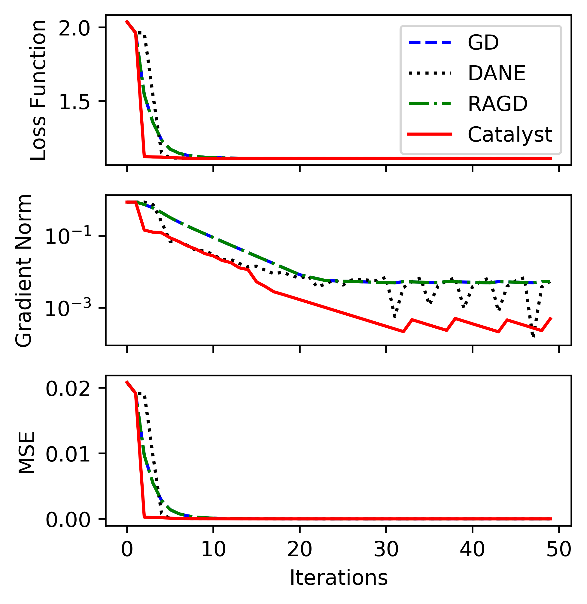
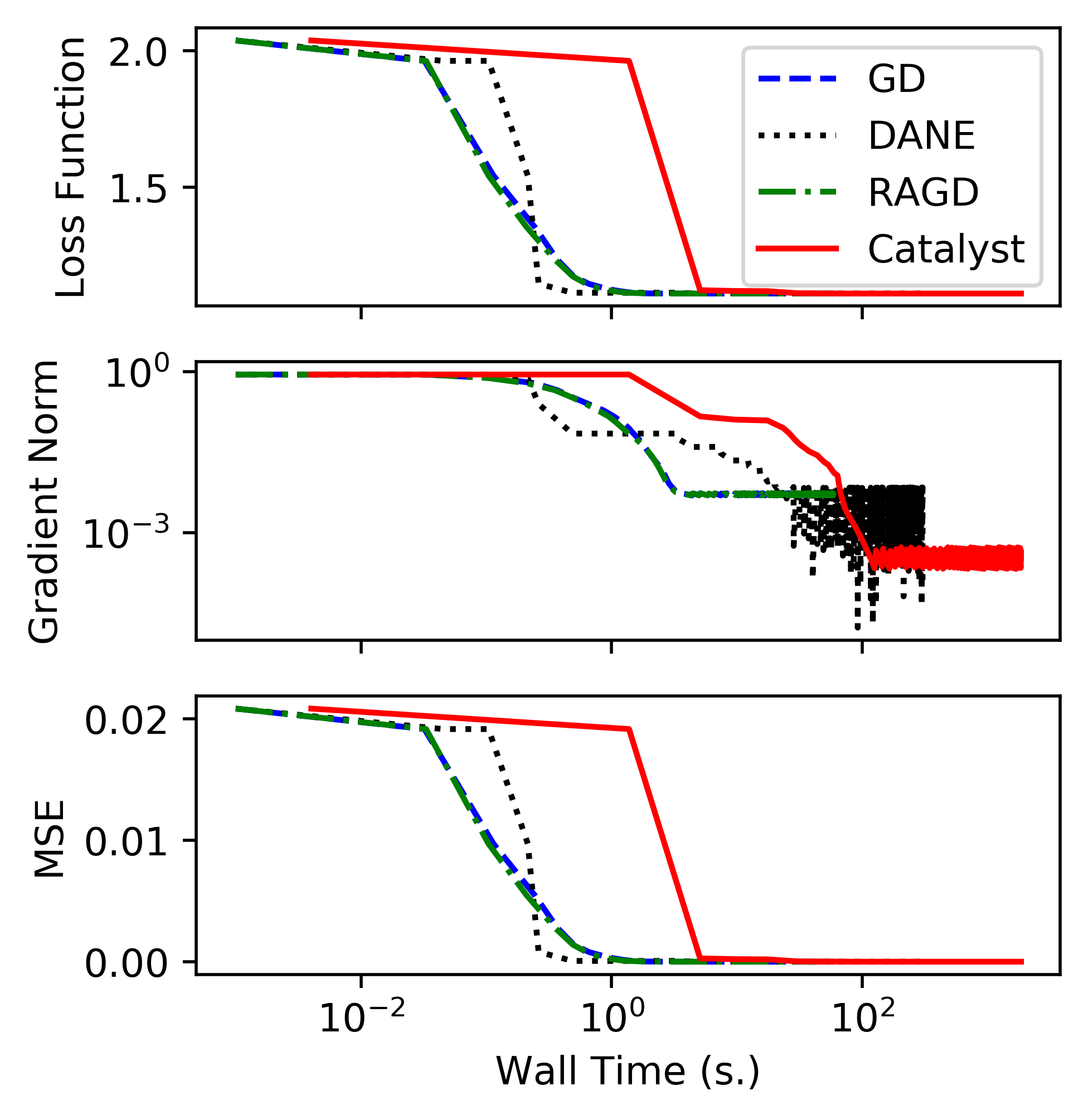
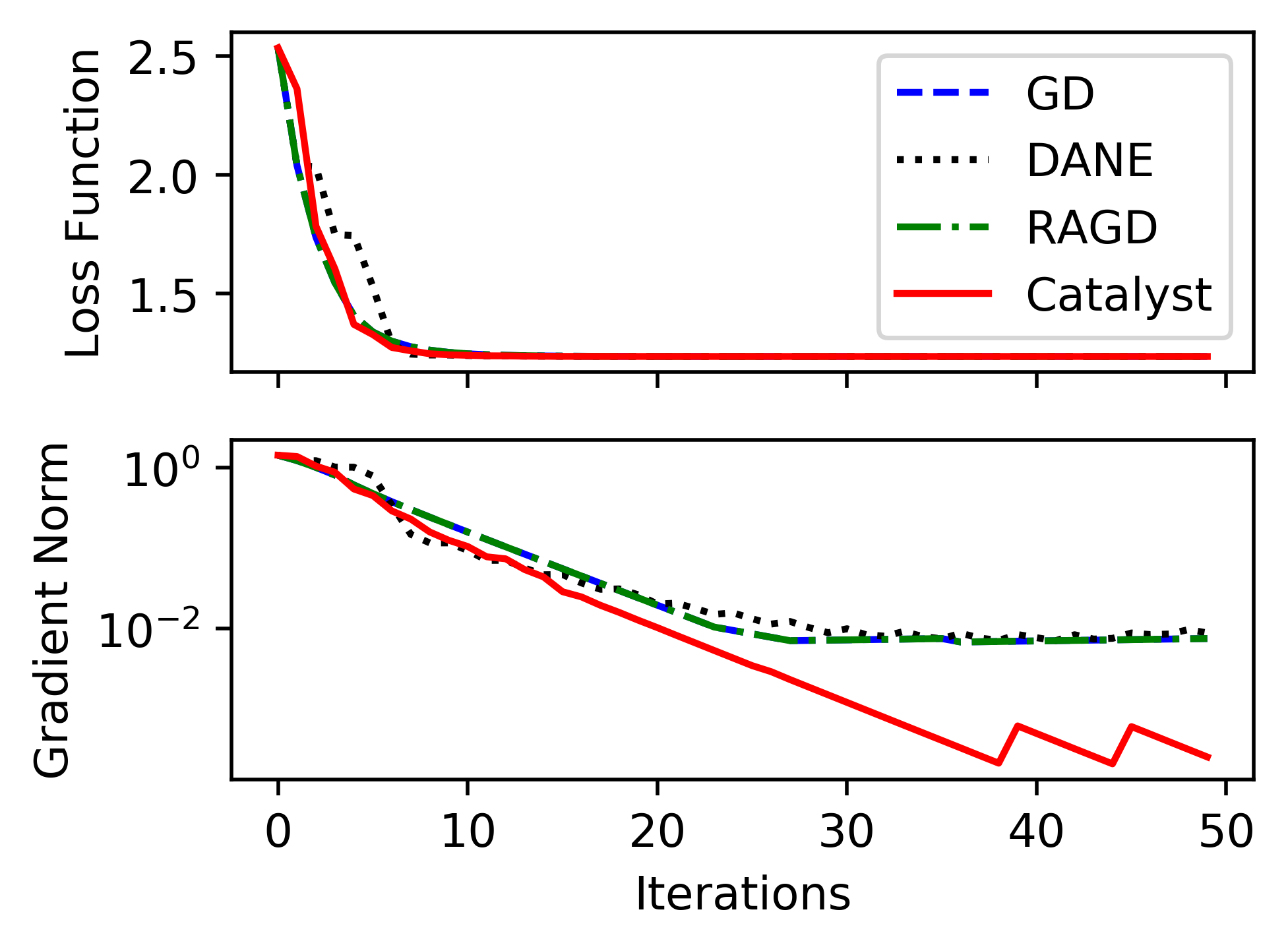
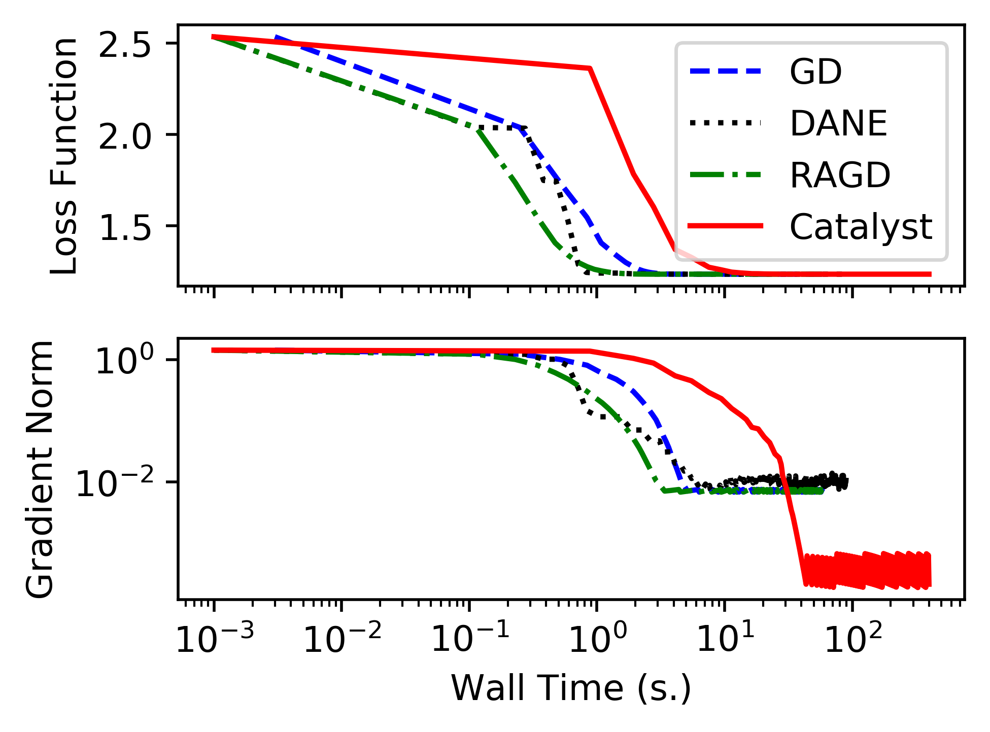
We first compare our accelerated method against gradient descent optimization and a Newton-type optimization scheme, DANE (Shamir et al.,, 2014), and a Nesterov method, RAGD (Zhang and Sra, 2018b, ), adapted for manifolds. For all the experiments in this section, we optimized the step size of the optimizer using an Armijo condition backtracing line seach (Armijo,, 1966) where we reduce the step size by a factor of $.95$ until the difference between the old loss function evaluation and the new one is $10^{-5}\times.95$. For our Catalyst algorithm manifold we set the A2 budget to $S=10$, the A1 number of iterations to $T=5$, and cutoff parameter for A1 is initialized at $.1$. For the DANE results, we set the regularization term to $1$, For RAGD we set the shrinkage parameter to $1$. Our synthetic data set is 10,000 observations generated i.i.d from a $100$ dimensional $\mbox{N}(0,I)$ distribution projected onto $\mathbb{S}^{99}$.

We run each optimization routine for 100 iterations. Figure 2 and Figure 3 shows that our novel accelerated method converges, for an intrinsic mean as well as an extrinsic mean example, to an optima in fewer iterations than the other competing methods, both in terms of the loss function value and the norm of the loss function gradient. Moreover, we can see in the intrinsic mean example, our method is able to obtain a smaller loss function and gradient norm than the competing methods. In the extrinsic mean example, our method obtains a comparable loss function value and MSE between the learned parameter and the closed-form expression of the sample mean with other methods in fewer iterations and obtains a smaller gradient norm than the competing methods.

By explicit calculation we show the objective functions are strongly convex over a neighborhood of any point on the manifold (see the Appendixx for a proof). This is a highly non-trivial task for general objective functions, hence necessitating an adaptive method such as ours. Moreover, in the extrinsic mean example, since we have a closed form expression of the Fréchet mean we also show that our optimization approach converges to the true extrinsic mean in terms of mean squared error faster than the other optimization methods.

Figure 2: Intrinsic mean comparison on spheres

Figure 3: Extrinsic mean comparison on spheres

4.2 Real data analysis: the Netflix example

Next, we consider an application of our algorithm to the Netflix movie rating dataset. This dataset of over a million entries, $X\in\mathbb{R}^{M\times N},$ consists of $M=17770$ movies and $N=480189$ users, in which only a sparse subset of the users and movies have ratings. In order to build a better recommendation systems to users, we can frame the problem of predicting users’ ratings for movies as a low-rank matrix completion problem by learning the rank-$r$ Grassmannian manifold $U\in\mbox{Gr(M, r)}$ which optimizes for the set of observed entries $(i,j)\in\Omega$ the loss function

$$L(U)=\frac{1}{2}\sum_{(i,j)\in\Omega}\left\{(UW)_{ij}-X_{ij}\right\}^{2}+\frac{\lambda^{2}}{2}\sum_{(i,j)\notin\Omega}(UW)_{ij},$$ (14)

where $W$ is an $r$-by-$N$ matrix. Each user $k$ has the loss function $\mathcal{L}(U,k)=\frac{1}{2}\left|c_{k}\circ\left(Uw_{k}(U)-X_{k}\right)\right|^{2}$ , where $\circ$ is the Hadamard product, $(w_{k})^{i}=W_{ik},$ and

$$\begin{split}(c_{k})^{i}=\begin{cases}1,&{\rm if}\ \ \ (i,k)\in\Omega\\ \lambda,&{\rm if}\ \ \ (i,k)\notin\Omega\end{cases},\qquad(X_{k})^{i}=\begin{cases}X_{ik},&{\rm if}\ \ \ (i,k)\in\Omega\\ 0,&{\rm if}\ \ \ (i,k)\notin\Omega,\end{cases}\\ w_{k}(U)=\big{(}U^{T}{\rm diag}(c_{k}\circ c_{k})U\big{)}^{-1}U^{T}\big{(}c_{k}\circ c_{k}\circ X_{k}\big{)}.\end{split}$$

This results in the following gradient

$$\nabla\mathcal{L}(U,k) =\big{(}c_{k}\circ c_{k}\circ(Uw_{k}(U)-X_{k})\big{)}w_{k}(U)^{T}$$

$$={\rm diag}(c_{k}\circ c_{k})(Uw_{k}(U)-X_{k})w_{k}(U)^{T}.$$

For this problem on Grassman manifolds, we have the retraction map:

$$\mathcal{R}_{V}U=U+V$$ (15)

and the inverse retraction map:

$$\mathcal{R}_{V}^{-1}U=V-U(U^{T}U)^{-1}U^{T}V$$ (16)

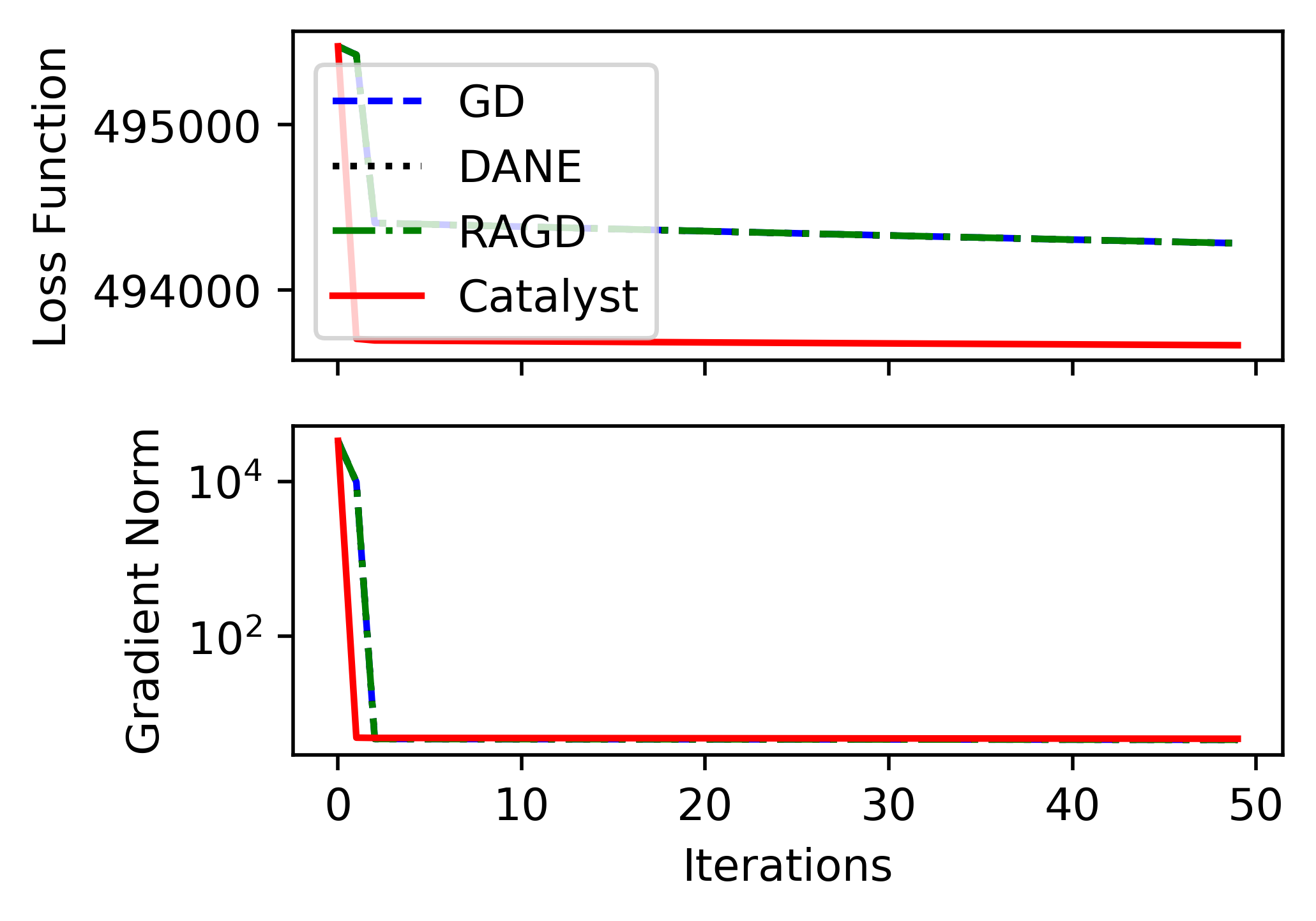
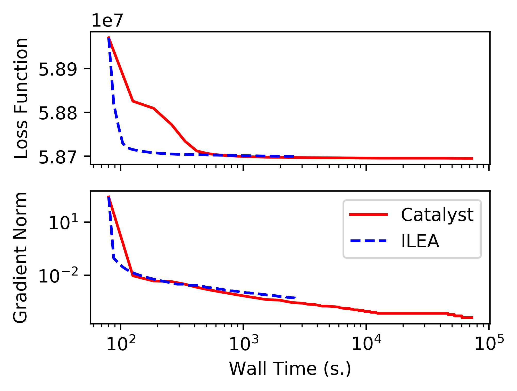
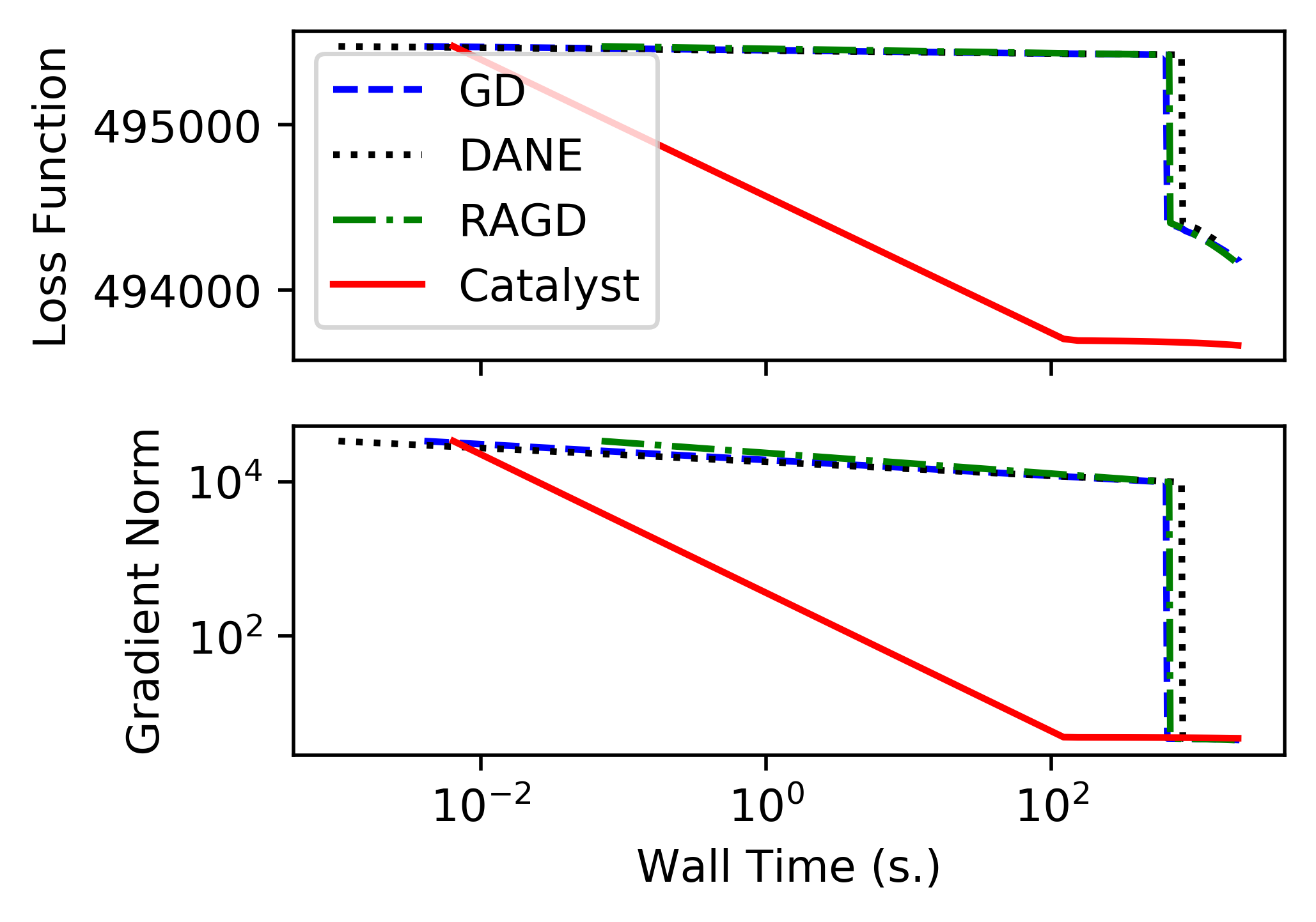
We look at a comparison of our method against a standard gradient descent method on a subset of the data where we only observe a million ratings ($\approx 1.5\%$ of the full data set). In this setting we fix the matrix rank $r=5$ and the regularization parameter $\lambda=.01$. Figure 4 shows that our accelerated method obtains a smaller loss function value, a smaller identical test set MSE, and nearly identical loss gradient norm faster than RAGD, DANE, or a typical gradient descent approach.

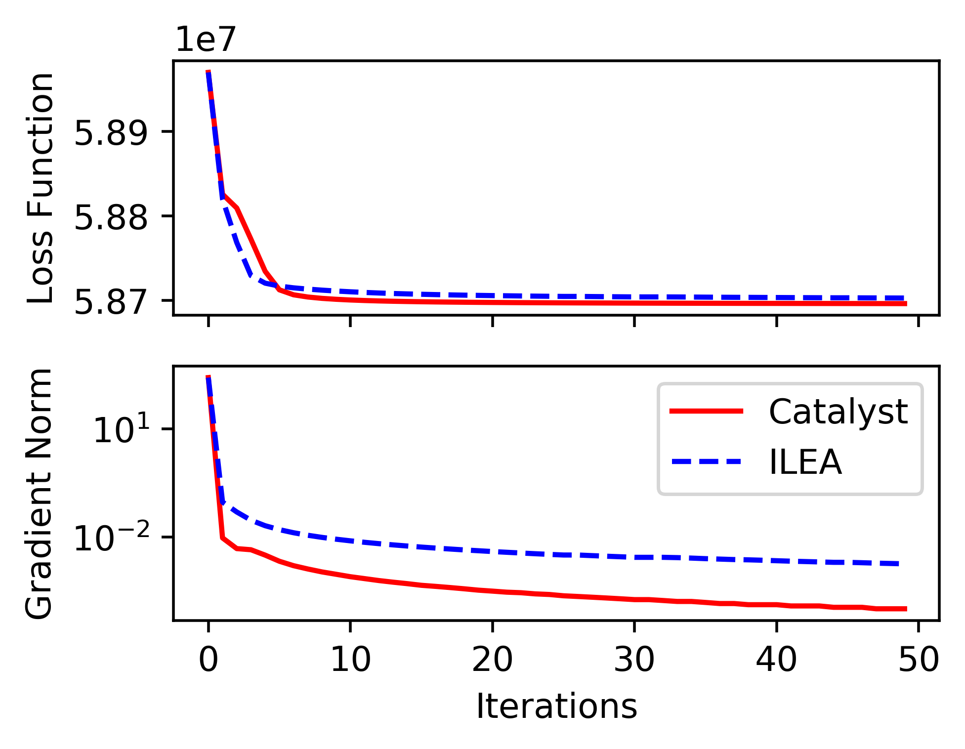
On a large scale, we apply a parallelized version of our accelerated method and a communication-efficient parallel algorithm on manifolds proposed in (Saparbayeva et al.,, 2018, ILEA) on the full Netflix dataset. We randomly distribute the data across 64 processors and run the optimization routine for 200 iterations. In Figure 4, again we can see steady acceleration that our method provides in terms of the loss function value across iterations and the loss of gradient norm though ILEA obtains slightly better test set MSE than our method.

Figure 4: Results for the parallel (right) and reduced (left) Netflix example.

.

5 Conclusion and Discussion

We propose a general scheme for solving non-convex optimization on manifolds which yields theoretical guarantees of convergence to a stationary point when the objective function is non-convex. When the objective function is convex, it leads to accelerated convergence rates for a large class of first order methods, which we show in our numerical examples. One of the interesting future directions we want to pursue is proposing accelerated algorithms on statistical manifolds (manifolds of densities or distributions) by employing information-geometric techniques, and applying the algorithms to accelerate convergence and mixing MCMC algorithms.

6 Appendix

6.1 Proof to Theorem 2

We first introduce a simple lemma.

Lemma 2.

Suppose the sequence $\{\alpha_{k}\}_{k\geq 1}$ is produced by $\mathcal{A}_{2}.$ Then, the following bounds hold for all $k\geq 1$

$$\frac{\sqrt{2}}{k+2}\leq\alpha_{k}\leq\frac{2}{k+1}.$$

Proof of Theorem 2.

The descent condition in

$$\begin{split}{\rm dist}\big{(}0_{\bar{\theta}_{k}},\partial h(\bar{\theta}_{k},\theta_{k-1})\big{)}&<\kappa_{k}d_{\mathcal{R}}(\bar{\theta}_{k},\theta_{k-1})\quad\text{and}\\ \quad h_{\kappa_{k}}(\bar{\theta}_{k},\theta_{k-1})&\leq h_{\kappa_{k}}(\theta_{k-1},\theta_{k-1}),\end{split}$$ (17)

implies $\{f(\theta_{k})\}_{k\geq 0}$ are monotonically decreasing. From this

$$\begin{split}f(\theta_{k-1})&=h_{\kappa}(\theta_{k-1},\theta_{k-1})\\ &\geq h_{\kappa}(\bar{\theta}_{k},\theta_{k-1})\\ &\geq f(\theta_{k})+\frac{\kappa}{2}d_{\mathcal{R}}^{2}(\bar{\theta}_{k},\theta_{k-1}).\end{split}$$ (18)

Using condition (17), we apply Lemma 2 with $\vartheta=\theta_{k-1},\theta=\bar{\theta}_{k}$ and $\varepsilon=\kappa Kd_{\mathcal{R}}(\bar{\theta}_{k},\theta_{k-1});$ hence

$${\rm dist}(0_{\bar{\theta}_{k}},\partial f(\bar{\theta}_{k}))\leq 2\kappa Kd_{\mathcal{R}}(\bar{\theta}_{k},\theta_{k-1}).$$

Combining the above inequality with (18), one has

$$\begin{split}{\rm dist}^{2}(0_{\bar{\theta}_{k}},\partial f(\bar{\theta}_{k}))&\leq 4\kappa^{2}K^{2}d_{\mathcal{R}}^{2}(\bar{\theta}_{k},\theta_{k-1})\\ &\leq 8\kappa_{\max}K^{2}\big{(}f(\theta_{k-1}-f(\theta_{k})\big{)}.\end{split}$$ (19)

Summing $j=1$ to $N,$ we can conclude

$$\min_{j=1,...,N}\Big{\{}{\rm dist}^{2}\big{(}0_{\bar{\theta}_{j}},\partial f(\bar{\theta}_{j})\big{)}\Big{\}} \leq\frac{8\kappa_{\max}K^{2}}{N}\sum^{N}_{j=1}\big{(}f(\theta_{j-1})-f(\theta_{j})\big{)}$$

$$\leq\frac{8\kappa_{\max}K^{2}}{N}\big{(}f(\theta_{0})-f^{*}\big{)}.$$

Fix an $v_{k}\in\partial h_{\kappa}(\tilde{\theta}_{k},\vartheta_{k}).$ Since the function $f$ is $\kappa_{cvx}(K_{1}^{4}K_{2}^{4}-R_{1})$-strongly convex, the function $h_{\kappa_{cvx}}$ is $\kappa_{cvx}K_{1}^{4}K_{2}^{4}$-strongly convex.

$$f(\theta) +\frac{\kappa_{cvx}}{2}d_{\mathcal{R}}^{2}(\theta,\vartheta_{k})$$

$$\geq f(\tilde{\theta}_{k})+\frac{\kappa_{cvx}}{2}d_{\mathcal{R}}^{2}(\tilde{\theta}_{k},\vartheta_{k})$$

$$\quad\quad+\frac{\kappa_{cvx}K_{1}^{4}K_{2}^{4}}{2}d_{\mathcal{R}}^{2}(\tilde{\theta}_{k},\theta)+\langle v_{k},\mathcal{R}_{\tilde{\theta}_{k}}^{-1}\theta\rangle.$$

Then

$$f(\tilde{\theta}_{k}) \leq f(\theta)+\frac{\kappa_{cvx}}{2}\big{(}d_{\mathcal{R}}^{2}(\theta,\vartheta_{k})-K_{1}^{4}K_{2}^{4}d_{\mathcal{R}}^{2}(\tilde{\theta}_{k},\theta)$$

$$\quad\quad-d_{\mathcal{R}}^{2}(\tilde{\theta}_{k},\vartheta_{k})\big{)}-\langle v_{k},\mathcal{R}_{\tilde{\theta}_{k}}^{-1}\theta\rangle.$$

So for any $\theta\in\mathcal{M}$

$$\begin{split}f(\theta_{k})\leq&f(\tilde{\theta}_{k})\\ \leq&f(\theta)+\frac{\kappa_{cvx}}{2}\Big{(}K_{1}^{2}\|\mathcal{R}^{-1}_{\theta_{k-1}}\theta-\mathcal{R}^{-1}_{\theta_{k-1}}\vartheta_{k}\|^{2}-K_{1}^{4}K_{2}^{2}\|\mathcal{R}^{-1}_{\theta_{k-1}}\tilde{\theta}_{k}\\ &-\mathcal{R}^{-1}_{\theta_{k-1}}\theta\|^{2}\Big{)}-\frac{\kappa_{cvx}}{2}d_{\mathcal{R}}^{2}(\tilde{\theta}_{k},\vartheta_{k})-\langle v_{k},\mathcal{R}_{\tilde{\theta}_{k}}^{-1}\theta\rangle.\end{split}$$

We substitute $\theta=\mathcal{R}_{\theta_{k-1}}\alpha_{k}\mathcal{R}^{-1}_{\theta_{k-1}}\theta^{*},$ where $\theta^{*}$ is any minimizer of $f.$ Using convexity of $f$

$$f(x)\leq\alpha_{k}f(\theta^{*})+(1-\alpha_{k})f(\theta_{k}),$$

the stopping criteria ,

$${\rm dist}\big{(}0_{\tilde{\theta}_{k}},\partial h_{\kappa_{cvx}}(\tilde{\theta}_{k},\vartheta_{k})\big{)}<\frac{\kappa_{cvx}}{k+1}d_{\mathcal{R}}(\tilde{\theta}_{k},\vartheta_{k}),$$ (20)

i.e. $\|v_{k}\|<\frac{\kappa_{cvx}}{k+1}d_{\mathcal{R}}(\tilde{\theta}_{k},\vartheta_{k}),$ and $\vartheta_{k}=\mathcal{R}_{\theta_{k-1}}\alpha_{k}\mathcal{R}^{-1}_{\theta_{k-1}}\tilde{\vartheta}_{k-1},$ and $\tilde{\vartheta}_{k}=\mathcal{R}_{\theta_{k-1}}\frac{1}{\alpha_{k}}\mathcal{R}^{-1}_{\theta_{k-1}}\tilde{\theta}_{k},$ one has

$$\begin{split}f(\theta_{k})\leq&\alpha_{k}f(\theta^{*})+(1-\alpha_{k})f(\theta_{k})\\ &+\frac{\kappa_{cvx}\alpha_{k}^{2}}{2}\Big{(}K_{1}^{2}\|\mathcal{R}^{-1}_{\theta_{k-1}}\theta^{*}-\mathcal{R}^{-1}_{\theta_{k-1}}\tilde{\vartheta}_{k-1}\|^{2}\\ &-K_{1}^{4}K_{2}^{2}\|\mathcal{R}^{-1}_{\theta_{k-1}}\tilde{\vartheta}_{k}-\mathcal{R}^{-1}_{\theta_{k-1}}\theta^{*}\|^{2}\Big{)}\\ &-\frac{\kappa_{cvx}}{2}d_{\mathcal{R}}^{2}(\tilde{\theta}_{k},\vartheta_{k})+\frac{\kappa_{cvx}}{k+1}d_{\mathcal{R}}(\tilde{\theta}_{k},\vartheta_{k})\|\mathcal{R}_{\tilde{\theta}_{k}}^{-1}\theta\|\\ \leq&\alpha_{k}f(\theta^{*})+(1-\alpha_{k})f(\theta_{k})\\ &+\frac{\kappa_{cvx}\alpha_{k}^{2}}{2}\Big{(}K_{1}^{2}K_{2}^{2}d_{\mathcal{R}}^{2}(\theta^{*},\tilde{\vartheta}_{k-1})-K_{1}^{2}K_{2}^{2}d_{\mathcal{R}}^{2}(\theta^{*},\tilde{\vartheta}_{k})\Big{)}\\ &-\frac{\kappa_{cvx}}{2}d_{\mathcal{R}}^{2}(\tilde{\theta}_{k},\vartheta_{k})+\frac{\kappa_{cvx}}{k+1}d_{\mathcal{R}}(\tilde{\theta}_{k},\vartheta_{k})d_{\mathcal{R}}(\tilde{\theta}_{k},\theta)\\ \leq&\alpha_{k}f(\theta^{*})+(1-\alpha_{k})f(\theta_{k})\\ &+\frac{\kappa_{cvx}\alpha_{k}^{2}}{2}\Big{(}K_{1}^{2}K_{2}^{2}d_{\mathcal{R}}^{2}(\theta^{*},\tilde{\vartheta}_{k-1})-K_{1}^{2}K_{2}^{2}d_{\mathcal{R}}^{2}(\theta^{*},\tilde{\vartheta}_{k})\Big{)}\\ &-\frac{\kappa_{cvx}}{2}d_{\mathcal{R}}^{2}(\tilde{\theta}_{k},\vartheta_{k})\\ &+\frac{\kappa_{cvx}K_{1}}{k+1}d_{\mathcal{R}}(\tilde{\theta}_{k},\vartheta_{k})\|\mathcal{R}_{\theta_{k-1}}^{-1}\tilde{\theta}_{k}-\mathcal{R}_{\theta_{k-1}}^{-1}\theta\|\\ =&\alpha_{k}f(\theta^{*})+(1-\alpha_{k})f(\theta_{k})\\ &+\frac{\kappa_{cvx}\alpha_{k}^{2}}{2}\Big{(}K_{1}^{2}K_{2}^{2}d_{\mathcal{R}}^{2}(\theta^{*},\tilde{\vartheta}_{k-1})-K_{1}^{2}K_{2}^{2}d_{\mathcal{R}}^{2}(\theta^{*},\tilde{\vartheta}_{k})\Big{)}\\ &-\frac{\kappa_{cvx}}{2}d_{\mathcal{R}}^{2}(\tilde{\theta}_{k},\vartheta_{k})\\ &+\frac{\kappa_{cvx}\alpha_{k}K_{1}}{k+1}d_{\mathcal{R}}(\tilde{\theta}_{k},\vartheta_{k})\|\mathcal{R}_{\theta_{k-1}}^{-1}\tilde{\vartheta}_{k}-\mathcal{R}_{\theta_{k-1}}^{-1}\theta^{*}\|\\ \leq&\alpha_{k}f(\theta^{*})+(1-\alpha_{k})f(\theta_{k})\\ &+\frac{\kappa_{cvx}\alpha_{k}^{2}}{2}\Big{(}K_{1}^{2}K_{2}^{2}d_{\mathcal{R}}^{2}(\theta^{*},\tilde{\vartheta}_{k-1})-K_{1}^{2}K_{2}^{2}d_{\mathcal{R}}^{2}(\theta^{*},\tilde{\vartheta}_{k})\Big{)}\\ &-\frac{\kappa_{cvx}}{2}d_{\mathcal{R}}^{2}(\tilde{\theta}_{k},\vartheta_{k})\\ &+\frac{\kappa_{cvx}\alpha_{k}K_{1}K_{2}}{k+1}d_{\mathcal{R}}(\tilde{\theta}_{k},\vartheta_{k})d_{\mathcal{R}}(\tilde{\vartheta}_{k},\theta^{*}).\end{split}$$

So

$$\begin{split}f(\theta_{k})\leq&\alpha_{k}f(\theta^{*})+(1-\alpha_{k})f(\theta_{k})\\ &+\frac{\kappa_{cvx}\alpha_{k}^{2}}{2}\Big{(}K_{1}^{2}K_{2}^{2}d_{\mathcal{R}}^{2}(\theta^{*},\tilde{\vartheta}_{k-1})-K_{1}^{2}K_{2}^{2}d_{\mathcal{R}}^{2}(\theta^{*},\tilde{\vartheta}_{k})\Big{)}\\ &-\frac{\kappa_{cvx}}{2}d_{\mathcal{R}}^{2}(\tilde{\theta}_{k},\vartheta_{k})\\ &+\frac{\kappa_{cvx}\alpha_{k}K_{1}K_{2}}{k+1}d_{\mathcal{R}}(\tilde{\theta}_{k},\vartheta_{k})d_{\mathcal{R}}(\theta^{*},\tilde{\vartheta}_{k}).\end{split}$$ (21)

Set $\mu_{k}=\frac{1}{k+1}.$ Completing the square yields

$$-\frac{\kappa_{cvx}}{2}d_{\mathcal{R}}^{2}(\tilde{\theta}_{k},\vartheta_{k})+\kappa_{cvx}\alpha_{k}\mu_{k}K_{1}K_{2}d_{\mathcal{R}}(\tilde{\theta}_{k},\vartheta_{k})d_{\mathcal{R}}(\theta^{*},\tilde{\vartheta}_{k})$$

$$\leq\frac{K_{1}^{2}K_{2}^{2}\kappa_{cvx}\alpha_{k}^{2}\mu_{k}^{2}}{2}d_{\mathcal{R}}^{2}(\theta^{*},\tilde{\vartheta}_{k}),$$

and subtracting $f^{*}=f(\theta^{*})$ from both sides, we obtain

$$\begin{split}f(\theta_{k})-f^{*}&\leq(1-\alpha_{k})(f(\theta_{k-1})-f^{*})+\frac{\kappa_{cvx}\alpha_{k}^{2}}{2}\Big{(}K_{1}^{2}K_{2}^{2}d_{\mathcal{R}}^{2}(\theta^{*},\tilde{\vartheta}_{k-1})\\ &\quad-K_{1}^{2}K_{2}^{2}d_{\mathcal{R}}^{2}(\theta^{*},\tilde{\vartheta}_{k})\Big{)}+\frac{K_{1}^{2}K_{2}^{2}\kappa_{cvx}\alpha_{k}^{2}\mu_{k}^{2}}{2}d_{\mathcal{R}}^{2}(\theta^{*},\tilde{\vartheta}_{k})\\ &=(1-\alpha)(f(\theta_{k-1})-f^{*})+\frac{\kappa_{cvx}\alpha_{k}^{2}K_{1}^{2}K_{2}^{2}}{2}d_{\mathcal{R}}^{2}(\theta^{*},\tilde{\vartheta}_{k-1})\\ &\quad-\frac{\kappa_{cvx}\alpha_{k}^{2}K_{1}^{2}K_{2}^{2}}{2}(1-\mu_{k}^{2})d_{\mathcal{R}}^{2}(\theta^{*},\tilde{\vartheta}_{k}).\end{split}$$

So one can obtain

$$\frac{f(\theta_{k})-f^{*}}{\alpha_{k}^{2}}+\frac{\kappa_{cvx}K_{1}^{2}K_{2}^{2}}{2}(1-\mu_{k}^{2})d_{\mathcal{R}}^{2}(\theta^{*},\tilde{\vartheta}_{k})$$

$$\leq\frac{1-\alpha_{k}}{\alpha_{k}^{2}}(f(\theta_{k-1})-f^{*})+\frac{\kappa_{cvx}K_{1}^{2}K_{2}^{2}}{2}d_{\mathcal{R}}^{2}(\theta^{*},\tilde{\vartheta}_{k-1}).$$

Denote $A_{k}=(1-\mu_{k}^{2}).$ Using the equality $\frac{1-\alpha_{k}}{\alpha_{k}^{2}}=\frac{1}{\alpha_{k-1}^{2}}$ we derive the following recursion

$$\begin{split}&\frac{f(\theta_{k})-f^{*}}{\alpha_{k}^{2}}+\frac{\kappa_{cvx}K_{1}^{2}K_{2}^{2}A_{k}}{2}d_{\mathcal{R}}^{2}(\theta^{*},\tilde{\vartheta}_{k})\\ &\leq\frac{1-\alpha_{k}}{\alpha_{k}^{2}}(f(\theta_{k-1})-f^{*})+\frac{\kappa_{cvx}K_{1}^{2}K_{2}^{2}}{2}d_{\mathcal{R}}^{2}(\theta^{*},\tilde{\vartheta}_{k-1})\\ &=\frac{f(\theta_{k-1})-f^{*}}{\alpha_{k-1}^{2}}+\frac{\kappa_{cvx}K_{1}^{2}K_{2}^{2}}{2}d_{\mathcal{R}}^{2}(\theta^{*},\tilde{\vartheta}_{k-1})\\ &\leq\frac{f(\theta_{k-1})-f^{*}}{A_{k-1}\alpha_{k-1}^{2}}+\frac{\kappa_{cvx}K_{1}^{2}K_{2}^{2}}{2}d_{\mathcal{R}}^{2}(\theta^{*},\tilde{\vartheta}_{k-1})\\ &=\frac{1}{A_{k-1}}\Bigg{(}\frac{f(\theta_{k-1})-f^{*}}{\alpha_{k-1}^{2}}+\frac{\kappa_{cvx}K_{1}^{2}K_{2}^{2}A_{k-1}}{2}d_{\mathcal{R}}^{2}(\theta^{*},\tilde{\vartheta}_{k-1})\Bigg{)}.\end{split}$$

The last inequality holds because $0<A_{k}\leq 1.$ Iterating $N$ times, we deduce

$$\frac{f(\theta_{N})-f^{*}}{\alpha_{N}^{2}} \leq\frac{f(\theta_{N})-f^{*}}{\alpha_{N}^{2}}+\frac{\kappa_{cvx}K_{1}^{2}K_{2}^{2}A_{k}}{2}d_{\mathcal{R}}^{2}(\theta^{*},\tilde{\vartheta}_{k})$$

$$\leq\frac{\kappa_{cvx}K_{1}^{2}K_{2}^{2}}{2}d_{\mathcal{R}}^{2}(\theta^{*},\theta_{0})\prod^{N}_{k=2}\frac{1}{A_{k-1}}.$$

Note that

$$\prod^{N}_{k=2}\frac{1}{A_{k-1}}\leq 2;$$

thereby with inequality from Lemma 1 we conclude

$$f(\theta_{N})-f^{*} \leq\frac{\alpha_{N}^{2}\kappa_{cvx}K_{1}^{2}K_{2}^{2}}{2}d_{\mathcal{R}}^{2}(\theta^{*},\theta_{0})\prod^{N}_{k=2}\frac{1}{A_{k-1}}$$

$$\leq\alpha_{N}^{2}\kappa_{cvx}K_{1}^{2}K_{2}^{2}d_{\mathcal{R}}^{2}(\theta^{*},\theta_{0})$$

$$\leq\frac{4\kappa_{cvx}K_{1}^{2}K_{2}^{2}}{(N+1)^{2}}d_{\mathcal{R}}^{2}(\theta^{*},\theta_{0}).$$

Hence

$$f(\theta_{N})-f^{*}\leq\frac{4\kappa_{cvx}K_{1}^{2}K_{2}^{2}}{(N+1)^{2}}d_{\mathcal{R}}^{2}(\theta^{*},\theta_{0}).$$

∎

6.2 Strong convexity of the objective function in estimating the intrinsic Fréchet means on the sphere

We provide a proof that the objective functions in estimating both the intrinsic and extrinsic Fréchet means on the sphere in Section 4 is strongly convex.

Proof.

In order to prove the strong-convexity of the intrinsic mean on the sphere $S^{n}$, we will prove the strong-convexity of the square intrinsic distance function from the point $x_{0}\in S^{n}$

$$d_{g}^{2}(x_{0},x)=\arccos^{2}(x_{0}^{T}x).$$

So for the geodesic from the point $x_{1}\in S^{n}$ to the point $x_{2}\in S^{2}$

$$\begin{split}\gamma(\lambda)&=\exp_{x_{1}}\lambda\log_{x_{1}}x_{2}\\ &=\cos\big{(}\lambda\arccos(x_{1}^{T}x_{2})\big{)}x_{1}\\ &\;\;+\sin\big{(}\lambda\arccos(x_{1}^{T}x_{2})\big{)}\frac{x_{2}-(x_{1}^{T}x_{2})x_{1}}{\sqrt{1-(x_{1}^{T}x_{2})^{2}}},\end{split}$$

we need to show following inequality

$$d_{g}^{2}(x_{0},\gamma(\lambda)) \leq(1-\lambda)d_{g}^{2}(x_{0},x_{1})+\lambda d_{g}^{2}(x_{0},x_{2})$$

$$\;\;-\frac{\lambda(1-\lambda)\mu}{2}d_{g}^{2}(x_{1},x_{2}).$$

For the sake of briefness let’s use the following notations

$$d_{1}=\arccos(x_{0}^{T}x_{1}),\qquad d_{2}=\arccos(x_{0}^{T}x_{2}),$$

$$d_{2}=\arccos(x_{1}^{T}x_{2}).$$

Therefore we have to prove the following inequality

$$\arccos^{2}\bigg{(}\cos(\lambda d_{3})\cos(d_{1})\\ +\sin(\lambda d_{3})\frac{\cos(d_{2})-\cos(d_{3})\cos(d_{1})}{\sin(d_{3})}\bigg{)}\\ \leq\quad(1-\lambda)d_{1}^{2}+\lambda d_{2}^{2}-\frac{\lambda(1-\lambda)\mu}{2}d_{3}^{2}.$$ (22)

Or we should prove the inequality

$$\arccos^{2}(x_{0}^{T}x_{2}) >\arccos^{2}(x_{0}^{T}x_{1})-2(\log_{x_{1}}x_{0})^{T}\log_{x_{1}}x_{2}$$

$$\;\;+\frac{\mu}{2}\arccos^{2}(x_{1}^{T}x_{2})$$

$$d_{2}^{2} >d_{1}^{2}-2\bigg{(}d_{1}\frac{x_{0}-\cos(d_{1})x_{1}}{\sin(d_{1})}\bigg{)}^{T}\bigg{(}d_{3}\frac{x_{2}-\cos(d_{3})x_{1}}{\sin(d_{3})}\bigg{)}+\frac{\mu}{2}d_{3}^{2}$$

$$=d_{1}^{2}-2d_{1}d_{3}\frac{\cos(d_{2})-\cos(d_{3})\cos(d_{1})}{\sin(d_{1})\sin(d_{3})}+\frac{\mu}{2}d_{3}^{2}$$

The last inequality was checked to hold in Wolfram Mathematica for $d_{1},d_{2}\in[0,\pi/4]$ and $d_{3}\in\Big{[}|d_{1}-d_{2}|,d_{1}+d_{2}\Big{]},$ where $\mu=1$.

In order to proof the strong-convexity of Fréchet function in estimating extrinsic mean on the sphere $S^{n}$, we will prove the strong-convexity of the square extrinsic distance function from the point $x_{0}\in S^{n}$

$$d_{e}^{2}(x_{0},x)=2(1-x_{0}^{T}x).$$

So for the geodesic from the point $x_{1}\in S^{n}$ to the point $x_{2}\in S^{2}$

$$\begin{split}\gamma(\lambda)&=\exp_{x_{1}}\lambda\log_{x_{1}}x_{2}\\ &=\cos\big{(}\lambda\arccos(x_{1}^{T}x_{2})\big{)}x_{1}+\sin\big{(}\lambda\arccos(x_{1}^{T}x_{2})\big{)}\frac{x_{2}-(x_{1}^{T}x_{2})x_{1}}{\sqrt{1-(x_{1}^{T}x_{2})^{2}}},\end{split}$$

we need to show that

$$d_{e}^{2}(x_{0},\gamma(\lambda)) \leq(1-\lambda)d_{e}^{2}(x_{0},x_{1})+\lambda d_{e}^{2}(x_{0},x_{2})$$

$$\;\;-\frac{\lambda(1-\lambda)\mu}{2}d_{g}^{2}(x_{1},x_{2}).$$

Therefore we have to prove

$$2\bigg{(}1-\cos(\lambda d_{3})\cos(d_{1})-\sin(\lambda d_{3})\frac{\cos(d_{2})-\cos(d_{3})\cos(d_{1})}{\sin(d_{3})}\bigg{)}\\ \leq\quad 2-2\big{(}(1-\lambda)\cos(d_{1})+\lambda\cos(d_{2})\big{)}-\frac{\lambda(1-\lambda)\mu}{2}d_{3}^{2}.$$ (23)

Or we need to show

$$2(1-x_{0}^{T}x_{2})>\\ 2(1-x_{0}^{T}x_{1})-2\big{(}x_{0}-(x_{0}^{T}x_{1})x_{1}\big{)}^{T}\log_{x_{1}}x_{2}+\frac{\mu}{2}\arccos^{2}(x_{1}^{T}x_{2})$$

Thus

$$2\big{(}1-\cos(d_{2})\big{)}$$

$$\quad\;>2\big{(}1-\cos(d_{1})\big{)}-2\big{(}x_{0}-\cos(d_{1})x_{1}\big{)}^{T}\bigg{(}d_{3}\frac{x_{2}-\cos(d_{3})x_{1}}{\sin(d_{3})}\bigg{)}+\frac{\mu}{2}d_{3}^{2}$$

$$\quad=2\big{(}1-\cos(d_{1})\big{)}-2d_{3}\frac{\cos(d_{2})-\cos(d_{3})\cos(d_{1})}{\sin(d_{3})}+\frac{\mu}{2}d_{3}^{2}$$

The last inequality was verified Wolfram Mathematica for $d_{1},d_{2}\in[0,\pi/4]$ and $d_{3}\in\Big{[}|d_{1}-d_{2}|,d_{1}+d_{2}\Big{]},$ where $\mu=1$

∎

Acknowledgments

Lizhen Lin would like to thank Dong Quan Nguyen for very helpful discussions. Lizhen Lin acknowledges the support from NSF grants IIS 1663870, DMS Career 1654579 and a DARPA grant N66001-17-1-4041. Bayan Saparbayeva was partially supported by DARPA N66001-17-1-4041.

References

• Absil et al., (2007) Absil, P.-A., Baker, C., and Gallivan, K. (2007). Trust-region methods on Riemannian manifolds. Foundations of Computational Mathematics, 7(3):303–330.
• Absil et al., (2010) Absil, P.-A., Mahony, R., and Sepulchre, R. (2010). Optimization on manifolds: methods and applications. In Diehl, M., Glineur, F., Jarlebring, E., and Michiels, W., editors, Recent Advances in Optimization and its Applications in Engineering, pages 125–144, Berlin, Heidelberg. Springer Berlin Heidelberg.
• Armijo, (1966) Armijo, L. (1966). Minimization of functions having Lipschitz continuous first partial derivatives. Pacific Journal of Mathematics, 16(1):1–3.
• Babanezhad et al., (2018) Babanezhad, R., Laradji, I. H., Shafaei, A., and Schmidt, M. O. (2018). Masaga: A linearly-convergent stochastic first-order method for optimization on manifolds. In ECML/PKDD.
• Bhattacharya and Bhattacharya, (2012) Bhattacharya, A. and Bhattacharya, R. (2012). Nonparametric Inference on Manifolds: With Applications to Shape Spaces. IMS Monograph #2. Cambridge University Press.
• Bhattacharya and Lin, (2017) Bhattacharya, R. and Lin, L. (2017). Omnibus CLTs for Fréchet means and nonparametric inference on non-Euclidean spaces. The Proceedings of the American Mathematical Society, 145:13–428.
• Bonnabel, (2013) Bonnabel, S. (2013). Stochastic gradient descent on Riemannian manifolds. IEEE Transactions on Automatic Control, 58(9):2217–2229.
• Boumal and Absil, (2011) Boumal, N. and Absil, P. (2011). RTRMC: A Riemannian trust-region method for low-rank matrix completion. In Shawe-Taylor, J., Zemel, R. S., Bartlett, P. L., Pereira, F., and Weinberger, K. Q., editors, Advances in Neural Information Processing Systems 24, pages 406–414. Curran Associates, Inc.
• Boumal et al., (2019) Boumal, N., Absil, P.-A., and Cartis, C. (2019). Global rates of convergence for nonconvex optimization on manifolds. IMA Journal of Numerical Analysis, 39(1):1–33.
• Edelman et al., (1998) Edelman, A., Arias, T., and Smith, S. (1998). The geometry of algorithms with orthogonality constraints. SIAM. J. Matrix Anal. & Appl., 20(2):303–353.
• Fréchet, (1948) Fréchet, M. (1948). Lés élements aléatoires de nature quelconque dans un espace distancié. Ann. Inst. H. Poincaré, 10:215–310.
• Huang and Gool, (2017) Huang, Z. and Gool, L. V. (2017). A Riemannian network for spd matrix learning. In AAAI.
• Huang et al., (2017) Huang, Z., Wan, C., Probst, T., and Gool, L. V. (2017). Deep learning on Lie groups for skeleton-based action recognition. 2017 IEEE Conference on Computer Vision and Pattern Recognition (CVPR), pages 1243–1252.
• Lin et al., (2017) Lin, H., Mairal, J., and Harchaoui, Z. (2017). Catalyst acceleration for first-order convex optimization: From theory to practice. J. Mach. Learn. Res., 18(1):7854–7907.
• Liu et al., (2017) Liu, Y., Shang, F., Cheng, J., Cheng, H., and Jiao, L. (2017). Accelerated first-order methods for geodesically convex optimization on Riemannian manifolds. In Guyon, I., Luxburg, U. V., Bengio, S., Wallach, H., Fergus, R., Vishwanathan, S., and Garnett, R., editors, Advances in Neural Information Processing Systems 30, pages 4868–4877. Curran Associates, Inc.
• Lohit and Turaga, (2017) Lohit, S. and Turaga, P. K. (2017). Learning invariant Riemannian geometric representations using deep nets. 2017 IEEE International Conference on Computer Vision Workshops (ICCVW), pages 1329–1338.
• Nesterov, (2004) Nesterov, Y. (2004). Introductory lectures on convex optimization: a basic course. Kluwer Academic Publishers.
• Nishimori et al., (2008) Nishimori, Y., Akaho, S., and Plumbley, M. D. (2008). Natural Conjugate Gradient on Complex Flag Manifolds for Complex Independent Subspace Analysis, pages 165–174. Springer Berlin Heidelberg, Berlin, Heidelberg.
• Paquette et al., (2018) Paquette, C., Lin, H., Drusvyatskiy, D., Mairal, J., and Harchaoui, Z. (2018). Catalyst for gradient-based nonconvex optimization. In Storkey, A. and Perez-Cruz, F., editors, Proceedings of the Twenty-First International Conference on Artificial Intelligence and Statistics, volume 84 of Proceedings of Machine Learning Research, pages 613–622, Playa Blanca, Lanzarote, Canary Islands. PMLR.
• Ring and Wirth, (2012) Ring, W. and Wirth, B. (2012). Optimization methods on Riemannian manifolds and their application to shape space. SIAM Journal on Optimization, 22(2):596–627.
• Saparbayeva et al., (2018) Saparbayeva, B., Zhang, M., and Lin, L. (2018). Communication efficient parallel algorithms for optimization on manifolds. In Bengio, S., Wallach, H., Larochelle, H., Grauman, K., Cesa-Bianchi, N., and Garnett, R., editors, Advances in Neural Information Processing Systems 31, pages 3574–3584. Curran Associates, Inc.
• Shamir et al., (2014) Shamir, O., Srebro, N., and Zhang, T. (2014). Communication-efficient distributed optimization using an approximate Newton-type method. In Proceedings of the 31st International Conference on International Conference on Machine Learning - Volume 32, ICML’14, pages II–1000–II–1008. JMLR.org.
• Smith, (2014) Smith, S. T. (2014). Optimization Techniques on Riemannian Manifolds. arXiv e-prints, page arXiv:1407.5965.
• Zhang et al., (2016) Zhang, H., Reddi, S. J., and Sra, S. (2016). Riemannian SVRG: Fast stochastic optimization on Riemannian manifolds. In Proceedings of the 30th International Conference on Neural Information Processing Systems, NIPS’16, pages 4599–4607, USA. Curran Associates Inc.
• Zhang and Sra, (2016) Zhang, H. and Sra, S. (2016). First-order methods for geodesically convex optimization. volume 49 of Proceedings of Machine Learning Research, pages 1617–1638, Columbia University, New York, New York, USA. PMLR.
• (26) Zhang, H. and Sra, S. (2018a). An estimate sequence for geodesically convex optimization. In Bubeck, S., Perchet, V., and Rigollet, P., editors, Proceedings of the 31st Conference On Learning Theory, volume 75 of Proceedings of Machine Learning Research, pages 1703–1723. PMLR.
• (27) Zhang, H. and Sra, S. (2018b). Towards Riemannian accelerated gradient methods. In 31th Annual Conference on Learning Theory.
• Zhang et al., (2018) Zhang, J., Zhang, H., and Sra, S. (2018). R-SPIDER: A fast Riemannian stochastic optimization algorithm with curvature Independent Rate. arXiv e-prints, page arXiv:1811.04194.
• Zhou et al., (2019) Zhou, P., Yuan, X.-T., and Feng, J. (2019). Faster first-order methods for stochastic non-convex optimization on Riemannian manifolds. In Chaudhuri, K. and Sugiyama, M., editors, Proceedings of Machine Learning Research, volume 89 of Proceedings of Machine Learning Research, pages 138–147. PMLR.