On the best choice of Lasso program given data parameters

Abstract

Generalized compressed sensing (GCS) is a paradigm in which a structured high-dimensional signal may be recovered from random, under-determined, and corrupted linear measurements. Generalized Lasso (GL) programs are effective for solving GCS problems due to their proven ability to leverage underlying signal structure. Three popular GL programs are equivalent in a sense and sometimes used interchangeably. Tuned by a governing parameter, each admit an optimal parameter choice. For sparse or low-rank signal structures, this choice yields minimax order-optimal error. While GCS is well-studied, existing theory for GL programs typically concerns this optimally tuned setting. However, the optimal parameter value for a GL program depends on properties of the data, and is typically unknown in practical settings. Performance in empirical problems thus hinges on a program’s parameter sensitivity: it is desirable that small variation about the optimal parameter choice begets small variation about the optimal risk. We examine the risk for these three programs and demonstrate that their parameter sensitivity can differ for the same data. We prove a gauge-constrained GL program admits asymptotic cusp-like behaviour of its risk in the limiting low-noise regime. We prove that a residual-constrained Lasso program has asymptotically suboptimal risk for very sparse vectors. These results contrast observations about an unconstrained Lasso program, which is relatively less sensitive to its parameter choice. We support the asymptotic theory with numerical simulations, demonstrating that parameter sensitivity of GL programs is readily observed for even modest dimensional parameters. Importantly, these simulations demonstrate regimes in which a GL program exhibits sensitivity to its parameter choice, though the other two do not. We hope this work aids practitioners in selecting a GL program for their problem.

I Introduction

Under-determined inverse problems are of fundamental importance to modern mathematical and machine learning applications. In these problems, one aims to recover or approximate a ground truth signal $x_{0}\in\mathbb{R}^{N}$ from noisy measurements $y\in\mathbb{R}^{m}$ when $m\ll N$. The paradigm of generalized compressed sensing (GCS) further specifies that the signal $x_{0}$ be well characterized by some structural proxy, known a priori, and that the measurement process be linear: $y=Ax_{0}+\eta z$, where $A\in\mathbb{R}^{m\times N}$ is typically random, and $z$ is either a random or deterministic corruption with noise scale $\eta>0$.

For example, in MR imaging, one may wish to recover the wavelet coefficients of an image by randomly subsampling its Fourier coefficeints [1, 2]. In geophysics, one may wish to determine a region’s bathymetry from a small number of radar measurements taken at the surface [3], or to obtain a subsurface image using a small number of geophones [4]. Recent investigations suggest how well-analyzed approaches for solving inverse problems may help to elucidate “mysterious” behaviours of high-dimensional non-linear function approximators [5, 6]. Moreover, compressed sensing theory may be used to prove recovery guarantees for certain neural network architectures and particular data regimes [7].

The now classical CS result [8] shows that when $x_{0}\in\mathbb{R}^{N}$ is an $s$-sparse signal, $m\geq Cs\log(eN/s)$ measurements suffice to efficiently recover $x_{0}$ from $(y,A)$ with high probability on the realization of $A$. The Lasso is a common and well-analyzed tool for effecting the recovery of $x_{0}$ [9, 10, 11, 8, 12, 13, 14]. Currently, “Lasso” is an umbrella term referring to three or more different Lasso programs, though it originally referred to the $\ell_{1}$-constrained program $(\mathrm{LS}_{\tau})$, which is defined below [13]. Effective for its ability to perform simultaneous best-basis and subset selection [13], the Lasso is a convex optimization approach that has several variants and cousins [9, 15, 16, 14].

Of particular interest to this work, we introduce three common Lasso programs and their solutions:

$$\hat{x}(\tau) \in\operatorname*{\arg\min}_{x\in\mathbb{R}^{N}}\big{\{}\|y-Ax\|_{2}^{2}:\|x\|_{1}\leq\tau\big{\}} \mathrm{LS}_{\tau}$$ ()

$$\tilde{x}(\sigma) \in\operatorname*{\arg\min}_{x\in\mathbb{R}^{N}}\big{\{}\|x\|_{1}:\|y-Ax\|_{2}^{2}\leq\sigma^{2}\big{\}} \mathrm{BP}_{\sigma}$$ ()

$$x^{\sharp}(\lambda) \in\operatorname*{\arg\min}_{x\in\mathbb{R}^{N}}\big{\{}\frac{1}{2}\|y-Ax\|_{2}^{2}+\lambda\|x\|_{1}\big{\}}. \mathrm{QP}_{\lambda}$$ ()

Some naming ambiguity for these programs exists in the literature. Here, we refer to $(\mathrm{LS}_{\tau})$ as constrained Lasso, $(\mathrm{QP}_{\lambda})$ as unconstrained Lasso, and $(\mathrm{BP}_{\sigma})$ as [quadratically constrained] basis pursuit; solutions for each program are denoted, respectively, by $\hat{x}(\tau)$, $\tilde{x}(\sigma)$ and $x^{\sharp}(\lambda)$. Our notation and naming convention for these three programs is similar to that used in [14].

Generalizations of these programs, commonly referred to as generalized Lasso, allow for the recovery of signals with other kinds of structure that are well modelled by convex proxy sets. To introduce the generalized Lasso programs, first let $\emptyset\neq\mathcal{K}\subseteq\mathbb{R}^{N}$ be a convex set and denote by $\|\cdot\|_{\mathcal{K}}$ the Minkowski functional of $\mathcal{K}$ (i.e., gauge). For $\sigma,\tau,\lambda>0$, the following generalized Lasso programs, which are convex, are defined by:

$$\hat{x}(\tau;A,y,\mathcal{K}) \in\operatorname*{\arg\min}_{x\in\mathbb{R}^{N}}\big{\{}\|y-Ax\|_{2}^{2}:x\in\tau\mathcal{K}\big{\}} \mathrm{LS}_{\tau,\mathcal{K}}$$ ()

$$\tilde{x}(\sigma;A,y,\mathcal{K}) \in\operatorname*{\arg\min}_{x\in\mathbb{R}^{N}}\big{\{}\|x\|_{\mathcal{K}}:\|y-Ax\|_{2}^{2}\leq\sigma^{2}\big{\}} \mathrm{BP}_{\sigma,\mathcal{K}}$$ ()

$$x^{\sharp}(\lambda;A,y,\mathcal{K}) \in\operatorname*{\arg\min}_{x\in\mathbb{R}^{N}}\big{\{}\frac{1}{2}\|y-Ax\|_{2}^{2}+\lambda\|x\|_{\mathcal{K}}\big{\}}. \mathrm{QP}_{\lambda,\mathcal{K}}$$ ()

In the standard CS setting, the gauge is the $\ell_{1}$-norm, though $x_{0}$ is assumed to belong to the set of $s$-sparse vectors $\Sigma_{s}^{N}:=\{x\in\mathbb{R}^{N}:|\operatorname{supp}(x)|\leq s\}$. So, $x_{0}$ does not necessarily belong to the convex proxy set $\mathcal{K}=B_{1}^{N}$, where $B_{1}^{N}$ denotes the $N$-dimensional unit $1$-norm ball. In particular, $B_{1}^{N}$ itself serves as a convex proxy set for sparse vectors in the sense that if $x\in\mathbb{R}^{N}$ is $s$-sparse, then $\|x\|_{1}/\|x\|_{2}$ is small relative to non-sparse vectors.

It is worth mentioning a brief note on uniqueness. When $A$ is under-determined and has a suitable randomness, it is straightforward to show the programs $(\mathrm{BP}_{\sigma})$ and $(\mathrm{QP}_{\lambda})$ admit unique solutions almost surely on the realization of $A$. A detailed exposition for $(\mathrm{QP}_{\lambda})$ is given in [17]. For a sufficient condition on $A$ giving uniqueness of $(\mathrm{BP}_{\sigma})$, see [18]. However, $(\mathrm{LS}_{\tau})$ does not always admit a unique solution. For instance, if $\tau$ is “too large”, then there may be infinitely many solutions $x\in\tau B_{1}^{N}$ satisfying $\|y-Ax\|_{2}=0$. This fact is fundamental to one of our results in §V. By mild abuse of notation, when the solution to a program is unique we will replace “$\in$” with “$=$” in the definitions of the solutions for each program. Otherwise, we define each of $\hat{x}(\tau),\tilde{x}(\sigma)$, and $x^{\sharp}(\lambda)$ as the solution yielding worst-case error, and which appears first when ordered lexicographically. For example, $\hat{x}(\tau)$ refers to the particular solution solving $(\mathrm{LS}_{\tau})$ such that $\|\hat{x}(\tau)-x_{0}\|_{2}\geq\|\hat{x}-x_{0}\|_{2}$ for any other $\hat{x}$ solving $(\mathrm{LS}_{\tau})$. We make an analogous modification to the definitions of the solutions to the generalized Lasso programs.

To relate the recovery performance of each program, we compare their recovery errors. While there are several possibilities for measuring the recovery error, the expected squared error and noise-normalized expected squared error of the estimator are common when the noise, $z$, is random [15]. In this work, we’ll define the loss for an estimator as the noise normalized squared error of that estimator (with respect to the ground truth signal $x_{0}$); and define the estimator’s risk as the expectation of the loss with respect to $z$. Note that the risk and loss are functions of the random matrix $A$. Specifically, the loss is defined for $(\mathrm{LS}_{\tau})$, $(\mathrm{BP}_{\sigma})$, $(\mathrm{QP}_{\lambda})$ respectively by:

$$\hat{L}(\tau;x_{0},A,\eta z) :=\eta^{-2}\|\hat{x}(\tau)-x_{0}\|_{2}^{2},$$

$$\tilde{L}(\sigma;x_{0},A,\eta z) :=\eta^{-2}\|\tilde{x}(\sigma)-x_{0}\|_{2}^{2},$$

$$L^{\sharp}(\lambda;x_{0},A,\eta z) :=\eta^{-2}\|\hat{x}(\eta\lambda)-x_{0}\|_{2}^{2},$$

and the risk by:

$$\hat{R}(\tau;x_{0},A,\eta) :=\operatorname{\mathbb{E}}_{z}\hat{L}(\tau;x_{0},A,\eta z)$$

$$\tilde{R}(\sigma;x_{0},A,\eta) :=\operatorname{\mathbb{E}}_{z}\tilde{L}(\sigma;x_{0},A,\eta z)$$

$$R^{\sharp}(\lambda;x_{0},A,\eta) :=\operatorname{\mathbb{E}}_{z}L^{\sharp}(\lambda;x_{0},A,\eta z).$$

Minimax order-optimal error rates are well-known for $\hat{x}(\tau;y,A,\mathcal{K})$ when $\tau$ is equal to the optimal parameter choice, $A$ is a matrix whose rows are independent, isotropic subgaussian random vectors, and $\mathcal{K}$ is a symmetric, closed convex set containing the origin [8, 19, 15]. A kind of equivalence between the three estimators (cf. §II) allows, in kind, for the characterization of the error rates for $\tilde{x}(\sigma)$ and $x^{\sharp}(\lambda)$ when $\sigma$ and $\lambda$ are optimally tuned. However, the error of $\hat{x}(\tau;y,A,\mathcal{K})$ is not fully characterized in the setting where $\tau$ is not the optimal choice. Similarly, the programs $(\mathrm{LS}_{\tau})$, $(\mathrm{BP}_{\sigma})$ and $(\mathrm{QP}_{\lambda})$ are often referred to interchangeably, but a full comparison of the error of the three estimators $\hat{x}(\tau),\tilde{x}(\sigma)$, and $x^{\sharp}(\lambda)$, as a function of their governing parameters, is lacking. It is an open question if there are settings in which one estimator is always preferable to another.

Understanding the sensitivity of a Lasso program to its parameter choice is crucial. While theoretical guarantees for recovery error are typically given for an oracular choice of the parameter, the optimal parameter setting is generally unknown in practice. Thus, the usefulness of theoretical recovery guarantees may hinge on the assumption that the recovery error is stable with respect to variation of the governing parameter. In particular, one may hope that small changes in the governing parameter beget no more than small changes in the risk or loss.

We take a step toward characterizing the performance and sensitivity of the three programs introduced by examining particular asymptotic parameter regimes for each program. We do this by extending results of [20, 21] from the setting where $A$ is identity to the setting where $A$ is a matrix whose rows are independent, isotropic subgaussian random vectors. In this setting, we prove the existence of regimes in which CS programs exhibit sensitivity to their parameter choice: small changes in parameter values can lead to blow-up in risk. Despite the notion of equivalence hinted at above, we demonstrate regimes in which one program exhibits sensitivity, while the other two do not. For example, in the very sparse regime, our theory and simulations suggest not to use $(\mathrm{BP}_{\sigma})$. In the low-noise regime, they suggest not to use $(\mathrm{LS}_{\tau})$. Assuredly, we identify situations where CS programs perform well in theory and in silico alike. We hope that the asymptotic theory, coupled with fairly extensive numerical simulations, aid practitioners in deciding which CS program to select.

II Summary of results to follow

As a way of alluding to the main results to follow, we start by describing three sibling results. We intend for them to contrast the behaviour of the three $\ell_{1}$ programs that are the main focus of this work. Define the worst-case risk for $(\mathrm{LS}_{\tau})$ in the low-noise regime by:

$$R^{*}(s,A):=\lim_{\eta\to 0}\sup_{x\in\Sigma_{s}^{N}\cap\partial B_{1}^{N}}\hat{R}(1;x,A,\eta)$$

Importantly, under mild assumptions, $R^{*}(s,A)$ is nearly equivalent to the optimally tuned worst-case risk for $(\mathrm{LS}_{\tau})$. Namely, for all $\eta>0$,

$$R^{*}(s,A)\leq\sup_{x\in\Sigma_{s}^{N}}\hat{R}(\|x\|_{1};x,A,\eta)\leq CR^{*}(s,A).$$

This result is treated formally in §IX-B. In each case discussed below, the performance of the estimators will be compared to $R^{*}(s,A)$ as a benchmark, noting that this quantity is minimax order optimal in the sense of §II.

In §V, we show that $(\mathrm{LS}_{\tau})$ exhibits an asymptotic instability in the low-noise regime. There is exactly one value $\tau^{*}$ of the governing parameter yielding minimax order-optimal error, with any choice $\tau\neq\tau^{*}$ yielding markedly worse behaviour. This result holds for normalized $K$-subgaussian matrices $A$, which are defined in Definition IV.3. The intuition provided by this result is that $(\mathrm{LS}_{\tau})$ is extremely sensitive to the value of $\tau$ in the low-noise regime, making empirical use of $(\mathrm{LS}_{\tau})$ woefully unstable in this regime.

Theorem II.1 ($(\mathrm{LS}_{\tau})$ instability simplified).

Let $1\leq s\leq m<N<\infty$ be integers. If $A\in\mathbb{R}^{m\times N}$ is a normalized $K$-subgaussian matrix with $m>C_{\varepsilon}\delta^{-2}K^{2}\log(K)s\log\left(\tfrac{N}{s}\right)$, then with probability at least $1-\varepsilon$ on the realization of $A$,

$$\lim_{\eta\to 0}\sup_{x\in\Sigma_{s}^{N}\cap B_{1}^{N}}\frac{\hat{R}(\tau;x,A,\eta)}{R^{*}(s,A)}=\begin{cases}1&\tau=1\\ \infty&\text{otherwise}\end{cases}$$

Next, in §VI we state a rephrasing of [22, Theorem 3]. The result shows there is a parameter $\lambda^{*}$ such that $(\mathrm{QP}_{\lambda})$ is not sensitive to its parameter choice for $\lambda\geq\lambda^{*}$. Right-sided parameter stability of $(\mathrm{QP}_{\lambda})$ was first established in [9, Theorem 7.2]. This well-known result is contrasted in §VIII with numerical results demonstrating a left-sided parameter instability for $(\mathrm{QP}_{\lambda})$ in the regime of high sparsity, low noise, and large dimension.

Theorem II.2 ($(\mathrm{QP}_{\lambda})$ right-sided stability).

Let $A\in\mathbb{R}^{m\times N}$ be a normalized $K$-subgaussian matrix for $1\leq m<N<\infty$. There is an absolute constant $C>0$ such that if $\lambda\geq C\sqrt{\log N}$ and $m\geq C_{\varepsilon}\delta^{-2}K^{2}\log(K)s\log\left(\tfrac{N}{s}\right)$, then with probability at least $1-\varepsilon$ on the realization of $A$,

$$R^{\sharp}(\lambda;x_{0},A,\eta)\leq C\lambda^{2}s.$$

In the initial work, $\lambda^{*}=2\sqrt{2\log N}$ [9, Theorem 7.2]. In the present phrasing, we write only that $\lambda^{*}=C\sqrt{\log N}$ for an absolute constant $C>0$. Note that when the data are Gaussian, right-sided stability of $(\mathrm{QP}_{\lambda})$ has been examined in [23]; of $(\mathrm{QP}_{\lambda,\mathcal{K}})$, in [16].

Finally, in §VII we show that $(\mathrm{BP}_{\sigma})$ is poorly behaved for all $\sigma>0$ when $x_{0}$ is very sparse. In particular, under mild restrictions on the aspect ratio of the measurement matrix, we show that $\tilde{R}(\sigma;x_{0},N,\eta)$ is asymptotically suboptimal for any $\sigma>0$ when $s/N$ is sufficiently small. Below, this theorem shows that the minimax risk for $(\mathrm{BP}_{\sigma})$, relative to the benchmark risk $R^{*}$, converges in probability to $\infty$.

Theorem II.3 ($(\mathrm{BP}_{\sigma})$ instability simplified).

Fix $\eta>0$, an integer $s\geq 1$, and suppose for $m:\mathbb{N}\to\mathbb{N}$ that $m(N)/N\to\gamma\in(0,1)$. For each $N$, suppose $A=A(N)\in\mathbb{R}^{m(N)\times N}$ is a normalized $K$-subgaussian matrix. Then, for all $M>0$,

$$\lim_{N\to\infty}\mathbb{P}\left(\inf_{\sigma>0}\sup_{x\in\Sigma_{s}^{N}}\frac{\tilde{R}(\sigma;x,A,\eta)}{R^{*}(s,A)}>M\right)=1.$$

Numerical results supporting §V and §VII are discussed in §VIII. Proofs of most of the theoretical results are deferred to §IX. Next, we add two clarifications. First, the three programs are equivalent in a sense.

Proposition (Program equivalence [8, Proposition 3.2]).

Let $0\neq x_{0}\in\mathbb{R}^{N}$ and $\lambda>0$. Where $x^{\sharp}(\lambda)$ solves $(\mathrm{QP}_{\lambda})$, define $\tau:=\|x^{\sharp}(\lambda)\|_{1}$ and $\sigma:=\|y-Ax^{\sharp}(\lambda)\|_{2}$. Then $x^{\sharp}(\lambda)$ solves $(\mathrm{LS}_{\tau})$ and $(\mathrm{BP}_{\sigma})$.

However, $\tau$ and $\sigma$ are functions of $z$, a random variable, and this mapping may not be smooth. Thus, parameter stability of one program is not implied by that of another. Second, $R^{*}(s,A)$ has the desirable property that it is computable up to multiplicative constants [19].

Proposition (Risk equivalences).

Fix $\delta,\varepsilon>0$, let $1\leq s\leq m<\infty,N\geq 2$ be integers, let $\eta>0$. Suppose $A\in\mathbb{R}^{m\times N}$ is a normalized $K$-subgaussian matrix satisfying $m>C_{\varepsilon}\delta^{-2}K^{2}\log Ks\log(N/s)$, and suppose that $y=Ax_{0}+\eta z$ for $z\in\mathbb{R}^{m}$ with $z_{i}\overset{\text{iid}}{\sim}\mathcal{N}(0,1)$. Let $M^{*}(s,N):=\inf_{x^{*}}\sup_{x_{0}\in\Sigma_{s}^{N}}\eta^{-2}\|x_{*}-x_{0}\|_{2}^{2}$ be the minimax risk over arbitrary estimators $x^{*}=x^{*}(y)$. With probability at least $1-\varepsilon$ on the realization of $A$, there is $c,C_{1},C_{\delta}>0$ such that

$$cs\log(N/s) \leq M^{*}(s,N)\leq\inf_{\lambda>0}\sup_{x_{0}\in\Sigma_{s}^{N}}R^{\sharp}(\lambda;x_{0},A,\eta)$$

$$\leq C_{\delta}R^{*}(s,A)\leq C_{\delta}s\log(N/s).$$

In this work, we focus primarily on the versions of Lasso for which $\|\cdot\|_{1}$ is the structural proxy, and $\Sigma_{s}^{N}$ the structure set for the data $x_{0}$. In addition, we discuss the pertinence of our results to the Generalized Lasso setting. For instance, in §A-A3, we show how Theorem V.1 adapts to setting of parameter sensitivity for low-rank matrix recovery using nuclear norm. Further, we connect our discussion on $(\mathrm{QP}_{\lambda})$ in §VI to results for more general gauges [23, 16], which works have developed tools suitable for analyzing parameter sensitivity of $(\mathrm{QP}_{\lambda,\mathcal{K}})$ when the data are Gaussian. While it remains an open question to determine how our results in §VII may be extended to analyze parameter sensitivity of $(\mathrm{BP}_{\sigma,\mathcal{K}})$, we conjecture that a suboptimality result like that exemplified in Theorem II.3 exists under analogous assumptions for $(\mathrm{BP}_{\sigma,\mathcal{K}})$.

III Related Work

Several versions of the Lasso program are well-studied in the context of solving CS problems [8]. The program $(\mathrm{LS}_{\tau})$ was first posed in [13]. An analysis of its risk when $\tau=\|x_{0}\|_{1}$ and the noise $z$ is deterministic may be found in [8]. A sharp non-asymptotic analysis for the generalized constrained Lasso may be found in [15]. There, the risk was shown to depend on specific geometric properties of the regularizer. When the measurement matrix has independent isotropic subgassian rows, it has been demonstrated how a geometric quantity may unify the quantification of generalized constrained Lasso risk [19]. Risk bounds for generalized constrained Lasso with nonlinear observations were characterized in [24]. Recent work has shown how dimensional parameters governing signal recovery problems in ridgeless least squares regression affect the average out-of-sample risk in some settings [5, 6].

Non-asymptotic bounds for the unconstrained Lasso were developed in [9], which also determines an order-optimal choice for the program’s governing parameter. The asymptotic risk for the unconstrained Lasso is determined analytically in [25, 26]. Sharp, non-asymptotic risk bounds for the generalized unconstrained Lasso are developed in [27, 23]. In [23], $R^{\sharp}(\lambda)$ is examined for $\lambda$ about $\lambda_{\mathrm{opt}}$, while [16] examines the risk as a function of its governing parameter for other kinds of $M$-estimators. Both assume Gaussianity of the data, and neither considers sensitivity with respect to parameter choice.

Basis pursuit is a third popular phrasing of the Lasso program, first proposed in [11, 10]. For a theoretical treatment of basis pursuit, we refer to [8]. Analytic connections between basis pursuit and other Lasso programs are exploited for fast computation of solutions in [14].

Other modifications of the standard Lasso have also been examined. For example, sharp non-asymptotic risk bounds for the so-called square-root Lasso were obtained in [15]. Related to basis pursuit, instance optimality of an exact $\ell_{1}$ decoder is analyzed in [28].

Sensitivity to parameter choice was analyzed for three proximal denoising (PD) programs that are analogues of the ones considered in this work [20, 21]. PD is a simplification of CS, in which $A$ is the identity matrix. There, the authors prove an asymptotic cusp-like behaviour for constrained PD risk in the low-noise regime, an asymptotic phase transition for unconstrained PD risk in the low-noise regime, and asymptotic suboptimality of the basis pursuit PD risk in the very sparse regime. The current work develops non-trivial generalizations of the results in [20], proving asymptotic results about the sensitivity of $\ell_{1}$ minimization for the generalized constrained Lasso, and generalized basis pursuit.

IV Main theoretical tools

IV-A Notation

Let $\operatorname{\mathrm{cvx}}(\mathcal{C})$ denote the convex hull of the set $\mathcal{C}\subseteq\mathbb{R}^{N}$:

$$\operatorname{\mathrm{cvx}}(\mathcal{C}) :=\{\sum_{j=1}^{J}\alpha_{j}x_{j}:x_{j}\in\mathcal{C},\alpha_{j}\geq 0,\sum\alpha_{j}=1,J<\infty\}$$

$$=\bigcap_{\mathclap{\begin{subarray}{c}\mathcal{C}^{\prime}\supseteq\mathcal{C}\\ \mathcal{C}^{\prime}\text{is convex}\end{subarray}}}\mathcal{C^{\prime}}.$$

Let $\operatorname{\mathrm{cone}}(\mathcal{C})$ denote the cone of $\mathcal{C}$:

$$\operatorname{\mathrm{cone}}(\mathcal{C}):=\{\lambda x:\lambda\geq 0,x\in\mathcal{C}\}.$$

Define the descent cone of a convex function $f:\mathbb{R}^{N}\to\mathbb{R}$ at a point $x\in\mathbb{R}^{N}$ by

$$T_{f}(x):=\operatorname{\mathrm{cone}}\{z-x:z\in\mathbb{R}^{N},f(z)\leq f(x)\}.$$

When $f=\|\cdot\|_{1}$ we write $T(x):=T_{\|\cdot\|_{1}}(x)$. By abuse of notation, we write $T_{\mathcal{C}}(x):=T_{\|\cdot\|_{\mathcal{C}}}(x)$ to refer to the descent cone of the gauge $\|\cdot\|_{\mathcal{C}}$ at a point $x$, where $\mathcal{C}\subseteq\mathbb{R}^{N}$ is a convex set.

Given $x\in\mathbb{R}^{N}$, denote the $0$-norm of $x$ by $\|x\|_{0}=\#\{j\in[N]:x_{j}\neq 0\}$, where $[N]:=\{1,2,\ldots,N\}$. Note that $\|\cdot\|_{0}$ is not a norm. For $0\leq p\leq\infty$, denote the $\ell_{p}$ ball by $B_{p}^{N}:=\{x\in\mathbb{R}^{N}:\|x\|_{p}\leq 1\}$. For $s,N\in\mathbb{N}$ with $0\leq s\leq N$, denote the set of at most $s$-sparse vectors by

$$\Sigma_{s}^{N}:=\{x\in\mathbb{R}^{N}:\|x\|_{0}\leq s\},$$

and define $\Sigma_{-1}^{N}:=\emptyset$. Define the following sets:

$$\mathcal{L}_{s}(r) :=r\cdot\operatorname{\mathrm{cvx}}(\Sigma_{s}^{N}\cap\mathbb{S}^{N-1}),$$

$$\mathcal{L}_{s} :=\mathcal{L}_{s}(2),$$

$$\mathcal{L}^{*}_{s} :=\mathcal{L}_{2s}(4).$$

Additionally, define the sets:

$$\mathcal{J}_{s}^{N} :=\left\{x\in\mathbb{R}^{N}:\|x\|_{1}\leq\sqrt{s}\|x\|_{2}\right\},$$

$$\mathcal{K}_{s}^{N} :=\left\{x\in\mathbb{R}^{N}:\|x\|_{2}\leq 1\,\And\,\|x\|_{1}\leq\sqrt{s}\right\}.$$

Observe that $\mathcal{J}_{s}^{N}$ is a cone, and that $\mathcal{K}_{s}^{N}=B_{2}^{N}\cap\sqrt{s}B_{1}^{N}=\operatorname{\mathrm{cvx}}(\mathcal{J}_{s}^{N}\cap\mathbb{S}^{N-1})$.

IV-B Tools from probability theory

We start by introducing subgaussian random variables, which generalize Gaussian random variables, but retain certain desirable properties, such as Gaussian-like tail decay and moment bounds.

Definition IV.1 (Subgaussian random variable).

A random variable $X$ is called subgaussian if there exists a constant $K>0$ such that the moment generating function of $X^{2}$ satisfies, for all $\lambda$ such that $|\lambda|\leq K^{-1}$,

$$\operatorname{\mathbb{E}}\exp(\lambda^{2}X^{2})\leq\exp(K^{2}\lambda^{2}).$$

The subgaussian norm of $X$ is defined by

$$\|X\|_{\psi_{2}}:=\inf\{t>0:\operatorname{\mathbb{E}}\exp(X^{2}/t^{2})\leq 2\}.$$

We similarly define subexponential random variables.

Definition IV.2 (Subexponential random variable).

A random variable $X$ is called subexponential if there exists a constant $K>0$ such that the moment generating function of $|X|$ satisfies, for all $\lambda$ such that $0\leq\lambda\leq K^{-1}$,

$$\operatorname{\mathbb{E}}\exp(\lambda|X|)\leq\exp(K\lambda).$$

The subexponential norm of $X$ is defined by

$$\|X\|_{\psi_{1}}:=\inf\{t>0:\operatorname{\mathbb{E}}\exp(|X|/t)\leq 2\}.$$

Additionally, we call $X\in\mathbb{R}^{N}$ a $K$-subgaussian random vector if $\|X\|_{\psi_{2}}:=\sup_{a\in\mathbb{R}^{N}}\|\langle a,X\rangle\|_{\psi_{2}}\leq K$; analogously so for $K$-subexponential random vectors. Where it is either clear or irrelevant, we may omit observing the norm parameter and refer to a $K$-subgaussian random vector simply as a subgaussian random vector; likewise with a subexponential random vector. For properties and equivalent definitions of subgaussian and subexponential random variables and vectors, see [29, Chapter 2]. Next, we introduce a piece of jargon for the sake of concision.

Definition IV.3 ($K$-subgaussian matrix).

Given $m,N\in\mathbb{N}$, call $A\in\mathbb{R}^{m\times N}$ a $K$-subgaussian matrix if $A$ has rows $A_{i}^{T}$ that are independent, isotropic $K$-subgaussian random vectors:

$$\operatorname{\mathbb{E}}A_{i}A_{i}^{T}=I,\qquad\|A_{i}\|_{\Psi_{2}}\leq K,\qquad i\in[m].$$

Further, call $\tfrac{1}{\sqrt{m}}A$ a normalized $K$-subgaussian matrix.

In this work, we crucially leverage the fact that $A$ satisfies a restricted isometry property (RIP). An exposition on RIP and restricted isometry constants may be found in [8]. As the results of this work concern $K$-subgaussian matrices, we state a classical version of RIP for such matrices restricted to the set of $s$-sparse vectors.

Theorem IV.1 (RIP for subgaussian matrices [8, Theorem 9.2]).

Let $A\in\mathbb{R}^{m\times N}$ be a normalized $K$-subgaussian matrix. There exists a constant $C=C_{K}>0$ such that the restricted isometry constant of $A$ satisfies $\delta_{s}\leq\delta$ with probability at least $1-\varepsilon$ provided

$$m\geq C\delta^{-2}(s\ln(eN/s)+\ln(2\varepsilon^{-1})).$$

Remark IV.1.

Setting $\varepsilon=2\exp(-\delta^{2}m/(2C))$ yields the condition

$$m\geq 2C\delta^{-2}s\ln(eN/s)$$

which guarantees that $\delta_{s}\leq\delta$ with probability at least $1-2\exp(-\delta^{2}m/(2C))$.

A tool necessary to the development of the results in §V and §VII (specifically §IX-C2, A-A4, and A-A4) characterizes the variance and tail decay of the supremum of a Gaussian process. For an introduction to random processes, we refer the reader to [29, 30].

Theorem IV.2 (Borell-TIS inequality [30, Theorem 2.1.1]).

Let $T$ be a topological space and let $\{f_{t}\}_{t\in T}$ be a centred (i.e., mean-zero) Gaussian process almost surely bounded on $T$ with

$${\left|\kern-1.07639pt\left|\kern-1.07639pt\left|f\right|\kern-1.07639pt\right|\kern-1.07639pt\right|}_{T} :=\sup_{t\in T}f_{t}, \sigma_{T}^{2} :=\sup_{t\in T}\operatorname{\mathbb{E}}\big{[}f_{t}^{2}\big{]}$$ (1)

such that ${\left|\kern-1.07639pt\left|\kern-1.07639pt\left|f\right|\kern-1.07639pt\right|\kern-1.07639pt\right|}_{T}$ is almost surely finite. Then $\operatorname{\mathbb{E}}{\left|\kern-1.07639pt\left|\kern-1.07639pt\left|f\right|\kern-1.07639pt\right|\kern-1.07639pt\right|}_{T}$ and $\sigma_{T}$ are both finite and for each $u>0$,

$$\mathbb{P}\big{(}{\left|\kern-1.07639pt\left|\kern-1.07639pt\left|f\right|\kern-1.07639pt\right|\kern-1.07639pt\right|}_{T}>\operatorname{\mathbb{E}}{\left|\kern-1.07639pt\left|\kern-1.07639pt\left|f\right|\kern-1.07639pt\right|\kern-1.07639pt\right|}_{T}+u\big{)}\leq\exp\big{(}-\frac{u^{2}}{2\sigma_{T}^{2}}\big{)}.$$

Observe that ${\left|\kern-1.07639pt\left|\kern-1.07639pt\left|f\right|\kern-1.07639pt\right|\kern-1.07639pt\right|}_{T}$ is notation; ${\left|\kern-1.07639pt\left|\kern-1.07639pt\left|\cdot\right|\kern-1.07639pt\right|\kern-1.07639pt\right|}_{T}$ is not a norm. By symmetry, one may derive an analogous lower-tail inequality. Consequently, one also has for each $u>0$,

$$\mathbb{P}\big{(}\left|{\left|\kern-1.07639pt\left|\kern-1.07639pt\left|f\right|\kern-1.07639pt\right|\kern-1.07639pt\right|}_{T}-\operatorname{\mathbb{E}}{\left|\kern-1.07639pt\left|\kern-1.07639pt\left|f\right|\kern-1.07639pt\right|\kern-1.07639pt\right|}_{T}\right|>u\big{)}\leq 2\exp\big{(}-\frac{u^{2}}{2\sigma_{T}^{2}}\big{)}.$$

IV-C Geometric tools from probability

Analysis of structured signals benefits from the ability to characterize their effective dimension. In this work, we capture this notion of effective dimension with the Gaussian complexity and Gaussian width (gw), which are closely related.

Definition IV.4 (Gaussian complexity).

Let $T\subseteq\mathbb{R}^{N}$. Define the Gaussian complexity of $T$ by

$$\gamma(T):=\operatorname{\mathbb{E}}\sup_{x\in T}\left|\langle x,g\rangle\right|,\qquad g\sim\mathcal{N}(0,I_{N}).$$

Definition IV.5 (Gaussian width).

Let $T\subseteq\mathbb{R}^{N}$. Define the Gaussian width of $T$, by:

$$\operatorname{w}(T):=\operatorname{\mathbb{E}}\sup_{x\in T}\langle x,g\rangle,\qquad g\sim\mathcal{N}(0,I_{N}).$$

Remark.

If $T$ is symmetric, then the gw of $T$ satisfies $\operatorname{w}(T)=\frac{1}{2}\operatorname{\mathbb{E}}\sup_{x\in T-T}\langle x,g\rangle$.

Next we state two results controlling the deviation of a $K$-subgaussian matrix on a bounded set, which generalize the idea of RIP introduced in Theorem IV.1. These results were first proved in [19], and an improved dependence on the constant $K$ was then obtained in [31]. The results are stated using the improved constant $\tilde{K}:=K\sqrt{\log K}$; we refer the reader to [31, Theorem 2.1] for further details.

Theorem IV.3 ([19, Theorem 1.1]).

Let $A\in\mathbb{R}^{m\times N}$ be a $K$-subgaussian matrix and $T\subseteq\mathbb{R}^{N}$ bounded. Then

$$\operatorname{\mathbb{E}}\sup_{x\in T}\left|\|Ax\|_{2}-\sqrt{m}\|x\|_{2}\right|\leq C\tilde{K}\gamma(T).$$

Another version of this result holds, where the deviation is instead controlled by the gw and radius, rather than the Gaussian complexity.

Theorem IV.4 ([19, Theorem 1.4]).

Let $A\in\mathbb{R}^{m\times N}$ be a $K$-subgaussian matrix and $T\subseteq\mathbb{R}^{N}$ bounded. For any $u\geq 0$ the event

$$\sup_{x\in T}\big{|}\|Ax\|_{2} -\sqrt{m}\|x\|_{2}\big{|}$$

$$\leq C\tilde{K}\left[\operatorname{w}(T)+u\cdot\operatorname{rad}(T)\right]$$ (2)

holds with probability at least $1-3\exp(-u^{2})$. Here, $\operatorname{rad}(T):=\sup_{x\in T}\|x\|_{2}$ denotes the radius of $T$.

Remark IV.2.

If $u\geq 1$ the bound in (IV.4) can be loosened to the following simpler one:

$$\sup_{x\in T}\left|\|Ax\|_{2}-\sqrt{m}\|x\|_{2}\right|\leq C\tilde{K}u\gamma(T).$$

Setting $T:=\mathbb{S}^{N-1}$, and using the improved constant obtained in [31, Theorem 2.1] gives the following corollary.

Corollary (Largest singular value of $K$-subgaussian matrices).

Let $A\in\mathbb{R}^{m\times N}$ be a $K$-subgaussian matrix. For all $t\geq 0$, with probability at least $1-3\exp(-t^{2})$,

$$\left|\|A\|-\sqrt{m}\right|\leq C\tilde{K}\left[\sqrt{N}+t\right].$$

Finally, we state the following comparison inequality for two centred Gaussian processes.

Theorem IV.5 (Sudakov-Fernique inequality [29, Theorem 7.2.11]).

Let $(X_{t})_{t\in T},(Y_{t})_{t\in T}$ be two mean-zero Gaussian processes. Assume that, for all $s,t\in T$, we have

$$\operatorname{\mathbb{E}}(X_{t}-X_{s})^{2}\leq\operatorname{\mathbb{E}}(Y_{t}-Y_{s})^{2}.$$

Then

$$\operatorname{\mathbb{E}}\sup_{t\in T}X_{t}\leq\operatorname{\mathbb{E}}\sup_{t\in T}Y_{t}.$$

IV-D Geometric tools

In this section, we introduce tools primarily relevant to obtaining recovery bounds for compressed sensing in the classical setting where $\mathcal{K}=B_{1}^{N}$. We start by recalling that sparse vectors have low effective dimension, as does their difference set.

Lemma (gw of the sparse signal set [32, Lemma 2.3]).

There exist absolute constants $c,C>0$ such that

$$cs\log(2N/s) \leq\operatorname{w}^{2}\left((\Sigma_{s}^{N}\cap B_{2}^{N})-(\Sigma_{s}^{N}\cap B_{2}^{N})\right)$$

$$\leq Cs\log(2N/s)$$

For possibly different absolute constants $c,C>0$, one also has

$$cs\log(2N/s)\leq\operatorname{w}^{2}\left(\Sigma_{s}^{N}\cap B_{2}^{N}\right)\leq Cs\log(2N/s).$$

In addition, we also recall that the descent cone of the $\ell_{1}$ ball has comparable effective dimension to the set of sparse vectors. For example, see [8, Proposition 9.24] for a related result showing $\operatorname{w}^{2}\left(T_{B_{1}^{N}}(x)\cap\mathbb{S}^{N-1}\right)\leq 2s\log(eN/s)$ when $x$ is $s$-sparse. To clarify the connection between the gw of $B_{1}^{N}$ and that of $\Sigma_{s}^{N}$, we recall the following result.

Lemma (Convexification [33, Lemma 3.1]).

One has

$$\operatorname{\mathrm{cvx}}(\Sigma_{s}^{N}\cap B_{2}^{N})\subseteq\mathcal{K}_{s}^{N}\subseteq 2\operatorname{\mathrm{cvx}}(\Sigma_{s}^{N}\cap B_{2}^{N}).$$

Next, it will be useful to leverage the following equivalent characterization for the $\ell_{1}$ descent cone. Recall that $\operatorname{\mathrm{sgn}}(\alpha):=1$ if $\alpha>0$, $\operatorname{\mathrm{sgn}}(\alpha)=-1$ if $\alpha<0$ and $\operatorname{\mathrm{sgn}}(0)=0$.

Lemma (Equivalent descent cone characterization).

Let $x\in\Sigma_{s}^{N}$ with non-empty support set $\mathcal{T}\subseteq[N]$ and define $\mathcal{C}:=\|x\|_{1}B_{1}^{N}$. If $K(x):=\{h\in\mathbb{R}^{N}:\|h_{\mathcal{T}^{C}}\|_{1}\leq-\langle\mathrm{sgn}(x),h\rangle\}$, then $T_{\mathcal{C}}(x)=K(x)$.

Finally, recall that Lasso solutions admit the following descent cone condition.

Lemma (Descent cone condition).

Let $x\in\Sigma_{s}^{N}$ have non-empty support set $T\subseteq N$. Suppose $y=Ax+\eta z$ for $\eta>0$, $z\in\mathbb{R}^{m}$, and $A\in\mathbb{R}^{m\times N}$. Let $\hat{x}$ solve $(\mathrm{LS}_{\tau})$ with $\tau=\|x\|_{1}$. Then $\|h\|_{1}\leq 2\sqrt{s}\|h\|_{2}$, where $h=\hat{x}-x$.

Proof of §IV-D.

We use §IV-D above before applying Cauchy-Schwarz:

$$\|\hat{x}-x\|_{1} =\|h_{T}\|_{1}+\|h_{T^{C}}\|_{1}$$

$$\leq\langle\mathrm{sgn}(\hat{x}_{T}-x),h_{T}\rangle-\langle\mathrm{sgn}(x),h\rangle$$

$$\leq\|\mathrm{sgn}(\hat{x}_{T}-x)-\mathrm{sgn}(x)\|_{2}\|h\|_{2}$$

$$\leq 2\sqrt{s}\|h\|_{2}.$$

∎

IV-E Refinements on bounds for gw

Crucial to the results of §VII are two recent results appearing in [34]. These results are a fine-tuning of standard gw results for bounded convex polytopes.

Proposition ([34, Proposition 1]).

Let $m\geq 1$ and $N\geq 2$. Let $T$ be the convex hull of $2N$ points in $\mathbb{R}^{m}$ and assume $T\subseteq B_{2}^{m}$. Then for $\gamma\in(0,1)$,

$$\operatorname{w} (T\cap\gamma B_{2}^{m})$$

$$\leq\min\big{\{}4\sqrt{\max\big{\{}1,\log(8eN\gamma^{2})\big{\}}},\gamma\sqrt{\min\{m,2N\}}\big{\}}$$

The work also proves a lower bound on the gw of bounded convex polytopes.

Proposition ([34]).

Let $m\geq 1$ and $N\geq 2$. Let $\gamma\in(0,1]$ and assume for simplicity that $s=1/\gamma^{2}$ is a positive integer such that $s\leq N/5$. Let $T$ be the convex hull of the $2N$ points $\{\pm M_{1},\ldots,\pm M_{N}\}\subseteq\mathbb{S}^{m-1}$. Assume that for some real number $\kappa\in(0,1)$ we have

$$\kappa\|\theta\|_{2}\leq\|M\theta\|_{2}\qquad\text{for all $\theta\in\mathbb{R}^{N}$ such that $\|\theta\|_{0}\leq 2s$},$$

Then

$$\operatorname{w}(T\cap\gamma B_{2}^{m})\geq(\sqrt{2}/4)\kappa\sqrt{\log(N\gamma^{2}/5)}.$$

In particular, the above two results may be combined to obtain a bound on a random polytope, obtained by considering the image of a (non-random) polytope under a normalized $K$-subgaussian matrix; proved in §A-A1.

Corollary (Controlling random hulls).

Fix $\delta,\varepsilon>0$, $\gamma\in(0,1]$ and let $A\in\mathbb{R}^{m\times N}$ be a normalized $K$-subgaussian matrix. Assume for simplicity that $s=1/\gamma^{2}\in\mathbb{N}$ with $s<N/5$ and let $T$ denote the convex hull of the $2N$ points $\{\pm A^{j}:j\in[N]\}$. Assume $m>C_{\varepsilon}\delta^{-2}\tilde{K}^{2}s\log(2N/s)$. With probability at least $1-\varepsilon$, for any $\alpha\in(0,(1-\delta))$,

$$(\sqrt{2}/4) (1-\delta)^{2}\sqrt{\log\frac{N\alpha^{2}}{5(1-\delta)^{2}}}$$

$$\leq\operatorname{w}(T\cap\alpha B_{2}^{m})$$

$$\leq\min\big{\{}4(1+\delta)\sqrt{\max\big{\{}1,\log\frac{8eN\alpha^{2}}{(1+\delta)^{2}}\big{\}}},$$

$$\qquad\qquad\alpha\sqrt{\min\{m,2N\}}\big{\}}.$$

IV-F Projection lemma

For $x\in\mathbb{R}^{N}$ and $\mathcal{C}\subseteq\mathbb{R}^{N}$ nonempty, denote the distance of $x$ to $\mathcal{C}$ by $\mathrm{dist}(x,\mathcal{C}):=\inf_{w\in\mathcal{C}}\|x-w\|_{2}$. If $\mathcal{C}$ is a closed and convex set, there exists a unique point in $\mathcal{C}$ attaining the infimum. We denote this point

$$\mathrm{P}_{\mathcal{C}}(x):=\operatorname*{\arg\min}_{w\in\mathcal{C}}\|x-w\|_{2}.$$

The projection lemma was an important tool in [20] for showing parameter instability of two Lasso programs in the proximal denoising setting. The result was first proved in [35, Lemma 15.3], and a simpler proof of a restated version given in [20]. The result shall play a critical role in this work, too. We include it here for completeness.

Lemma (Projection lemma [20, Lemma 3.2]).

Let $\mathcal{K}\subseteq\mathbb{R}^{m}$ be a non-empty closed and convex set with $0\in\mathcal{K}$, and fix $\lambda\geq 1$. Then, for any $z\in\mathbb{R}^{m}$,

$$\|\mathrm{P}_{\mathcal{K}}(z)\|_{2}\leq\|\mathrm{P}_{\lambda\mathcal{K}}(z)\|_{2}.$$

§IV-F admits the following corollary, useful in proving §IX-D2. Its proof is deferred to §A-A2.

Corollary ([20, Corollary 3.1]).

Let $\mathcal{K}\subseteq\mathbb{R}^{m}$ be a non-empty closed and convex set with $0\in\mathcal{K}$ and let $\|\cdot\|_{\mathcal{K}}$ be the gauge of $\mathcal{K}$. Given $y\in\mathbb{R}^{m}$, define for $\alpha>0$,

$$q_{\alpha}:=\operatorname*{\arg\min}\{\|q\|_{\mathcal{K}}:\|q-y\|_{2}\leq\alpha\}.$$

Then $\|q_{\alpha}\|_{2}$ is decreasing in $\alpha$.

V $(\mathrm{LS}_{\tau})$ parameter instability

The main result of this section is proved in the case of standard CS, where $x_{0}\in\Sigma_{s}^{N}$ and where tight bounds on the effective dimension of the structure set are known (e.g., bounds on $\gamma(\mathcal{L}_{s})$ or $\gamma(\mathcal{K}_{s}^{N})$). Define $\tau^{*}:=\|x_{0}\|_{1}$. The following result states that $\hat{L}$ is almost surely suboptimal in the limiting low-noise regime when $\tau\neq\tau^{*}$, while $\hat{R}(\tau^{*})$ is order-optimal. A proof of the result may be found in §IX-C3, with supporting lemmas in §IX-C.

Theorem V.1 (Asymptotic singularity).

Fix $\delta,\varepsilon>0$ and let $1\leq s\leq m<N<\infty$ be integers. Let $x_{0}\in\Sigma_{s}^{N}\setminus\Sigma_{s-1}^{N}$ with $\tau^{*}:=\|x_{0}\|_{1}$ and $\tau>0$ such that $\tau\neq\tau^{*}$. Let $\eta>0$ and let $z\in\mathbb{R}^{m}$ with $z_{i}\overset{\text{iid}}{\sim}\mathcal{N}(0,1)$. Suppose $A\in\mathbb{R}^{m\times N}$ is a normalized $K$-subgaussian matrix, and assume $m$ satisfies

$$m>C_{\varepsilon}\tilde{K}^{2}\delta^{-2}s\log\frac{eN}{s}.$$

Almost surely on the realization of $(A,z)$,

$$\lim_{\eta\to 0}\hat{L}(\tau;x_{0},A,\eta z)=\infty.$$

With probability at least $1-\varepsilon$ on the realization of $A$, there exist constants $0<c_{\delta}<C_{\delta}<\infty$ such that

$$c_{\delta}s\log\frac{N}{s}\leq\lim_{\eta\to 0}\sup_{x\in\Sigma_{s}^{N}}\hat{R}(\|x\|_{1};x,A,\eta)\leq C_{\delta}s\log\frac{N}{2s}.$$

For clarity, observe the similarity to the definition of $\tau^{*}$ of the precise parameter, $\|x\|_{1}$, appearing in the lower bound. Importantly, the spirit of this result extends to the situation where $x_{0}$ belongs, more generally, to some convex proxy set $\mathcal{K}\subseteq\mathbb{R}^{N}$. In particular, the blow-up of $\hat{L}$ in the limiting low-noise regime holds independent of the assumptions on $\mathcal{K}$, except that $\mathcal{K}$ be bounded. For instance, §A-A3 addresses the an analogous result in the case where the signal is a $d\times d$ matrix and $\mathcal{K}$ is the nuclear norm ball. Further, worst-case bounds on $\hat{R}$ are well-known in the case where $\mathcal{K}$ is a convex polytope, and are useful when $\mathcal{K}$ has small gw [34, 19].

VI Analysis of $(\mathrm{QP}_{\lambda})$

VI-A Right-sided parameter stability

In this section we present a contrast to the type of sensitivity observed in §V. Specifically, the result serves to demonstrate that $(\mathrm{QP}_{\lambda})$ is not sensitive to its parameter choice if the chosen parameter is too large. This so-called right-sided parameter stability is important in practical settings, as it suggests that recovery will not be penalized “too heavily” if the parameter is chosen incorrectly to be too large. Having such a leniency is reassuring, since knowing the exact choice of $\lambda$ in an experimental setting is unlikely at best.

The right-sided parameter stability for $(\mathrm{QP}_{\lambda})$ was first proved in [9, Theorem 7.2]. When the data are Gaussian, right-sided stability of $(\mathrm{QP}_{\lambda})$ has been examined in [23]; of $(\mathrm{QP}_{\lambda,\mathcal{K}})$, in [16]. Here, we state a specialized rephrasing of a version more suitably adapted to the present work [22, Theorem 3]. This version is the same as that stated in §II.

Theorem VI.1 (Specialized [22, Theorem 3]).

For integers $1\leq s\leq m<N<\infty$, suppose $x_{0}\in\Sigma_{s}^{N}$ and let $A\in\mathbb{R}^{m\times N}$ be a normalized $K$-subgaussian matrix. There is an absolute constant $C>0$ such that if $\lambda\geq C\sqrt{\log N}$ and $m\geq C_{\varepsilon}\tilde{K}^{2}\delta^{-2}s\log\tfrac{N}{s}$, then with probability at least $1-\varepsilon$ on the realization of $A$,

$$R^{\sharp}(\lambda;x_{0},A,\eta)\leq Cs\lambda^{2}.$$

In particular, over-guessing $\lambda$ results in no more than a quadratic penalty on the bound for the recovery error. Consequently, $(\mathrm{QP}_{\lambda})$ is right-sided parameter stable — it is not sensitive to variation of its governing parameter when the parameter is sufficiently large. We note, thereby, that there exist regimes in which Lasso programs are not sensitive to their parameter choice. Perhaps more importantly: there are regimes in which one program may be sensitive to its parameter choice, and another program is not. Namely, we see that $(\mathrm{LS}_{\tau})$ can be sensitive to its parameter choice in the low-noise regime (so the correct choice of $\tau$ is an imperative), while recovery for the very same data using $(\mathrm{QP}_{\lambda})$ is not sensitive to $\lambda$ (if $\lambda$ is sufficiently large enough).

VII Analysis of $(\mathrm{BP}_{\sigma})$

The final program that we subject to scrutiny is $(\mathrm{BP}_{\sigma})$. It is well-known under standard assumptions that an optimal choice of $\sigma$ yields order-optimal risk $\tilde{R}(\sigma^{*};x_{0},A,\eta)$ with high probability on the realization of $A$. In this section, we demonstrate the existence of a regime in which any choice of $\sigma$ fails to yield order-optimal recovery for $(\mathrm{BP}_{\sigma})$. A key message of this section is that $(\mathrm{BP}_{\sigma})$ performs poorly if the signal is too sparse and the number of measurements is too large. We demonstrate this behaviour for two regimes: the underconstrained setting, where $\sigma$ is “too large” and the overconstrained setting where $\sigma$ is “too small”. Each of these settings covers the case where $\sigma$ is chosen “just right”; we will see how $(\mathrm{BP}_{\sigma})$ risk fails to achieve order optimality in this case, as well.

For the duration of this section, we will consider $x_{0}\in\Sigma_{s}^{N}$ where $s$ may or may not be allowed to be $0$. We will clarify this explicitly in each instance. The main result of the section will be stated in the case where $A\in\mathbb{R}^{m\times N}$ is a normalized $K$-subgaussian matrix whose rows $m=m(N)$ satisfying a particular growth condition. Thus, the measurement vector will be given by $y=Ax_{0}+\eta z$ where $\eta>0$ is the noise scale and $z_{i}\overset{\text{iid}}{\sim}\mathcal{N}(0,1)$ as before. For the sake of analytical and notational simplicity, we assume that $\eta$ is independent of $N$. However, we eventually make clear how $\sigma$ may be allowed to depend on the ambient dimension, and that our result holds irrespective of this dependence.

VII-A Underconstrained parameter instability

As a “warm-up” for the main result, we start by demonstrating that there is a regime in which $\tilde{R}(\sigma;x_{0},A,\eta)$ fails to achieve minimax order-optimality when restricted to $\sigma\geq\eta\sqrt{m}$. Specifically, if $m$ is too large, then there is a (sufficiently sparse) vector $x_{0}\in\Sigma_{s}^{N}$ such that, with high probability on the realization of $A$, the risk $\tilde{R}(\sigma;x_{0},A,\eta)$ is large regardless of the choice of $\sigma\in[\eta\sqrt{m},\infty)$. We defer the proof of this result to §IX-D1.

Lemma (Underconstrained maximin $(\mathrm{BP}_{\sigma})$).

Fix $\delta,\varepsilon,\eta>0$, let $1\leq s<m\leq N$ be integers, and suppose $A\in\mathbb{R}^{m\times N}$ is a normalized $K$-subgaussian matrix. If

$$m>C_{\varepsilon}\delta^{-2}\tilde{K}^{2}s^{2}\log^{2}\left(\frac{N}{s}\right),$$

then with probability at least $1-\varepsilon$ on the realization of $A$,

$$\inf_{\sigma\geq\eta\sqrt{m}}\sup_{x\in\Sigma_{s}^{N}}\tilde{R}(\sigma;x,A,\eta)\geq C\sqrt{m}.$$

Remark VII.1.

In some settings, it may be not be appropriate for $m$ to depend logarithmically on $N$. If $m$ and $N$ satisfy the power law relation $m=N^{k}$ for some $k>0$, then under the assumptions of §VII-A,

$$\operatorname{\mathbb{E}}_{z}\|\tilde{x}(\sigma)-x_{0}\|_{2}^{2}=\Omega(N^{k/2}).$$

VII-B Minimax suboptimality

Just as observed in §VII-A, the results of this section hold in the regime where the aspect ratio approaches a constant: $m/N\to\gamma\in(0,1)$. Our simulations in §VIII-C support suboptimality of $\tilde{R}$, and sensitivity of $(\mathrm{BP}_{\sigma})$ to its parameter choice for aspect ratios ranging from $\gamma=0.1$ to $\gamma=0.45$.

Our result is of an asymptotic nature in one additional sense. We have stated that $\tilde{R}$ may be suboptimal for “very sparse” signals $x_{0}$. This is specified in the sense that, while $m$ and $N$ may be allowed to grow, $s$ remains fixed. Our numeric simulations demonstrate how this assumption may be interpreted as the inability of $(\mathrm{BP}_{\sigma})$ to effectively recover the off-support of the signal $x_{0}$ (i.e., the all $0$ sub-vector $x_{T^{C}}$ where $T\subseteq[N]$ denotes the support of $x_{0}$). Thus, it is in this setting, where the number of measurements is sufficiently large, and the sparsity sufficiently small, that we show $\tilde{R}(\sigma;x_{0},A,\eta)$ is asymptotically suboptimal, regardless of the choice of $\sigma$.

Theorem VII.1 ($(\mathrm{BP}_{\sigma})$ minimax suboptimality).

Fix $\varepsilon,\eta>0$ and $m:\mathbb{N}\to\mathbb{N}$ with $m(N)/N\to\gamma\in(0,1)$. There is $N_{0}\geq 2$ and $p>0$ so that for any $N\geq N_{0}$ and any $1\leq s<m(N_{0})$, if $A\in\mathbb{R}^{m\times N}$ is a normalized $K$-subgaussian matrix, then with probability at least $1-\varepsilon$ on the realization of $A$,

$$\inf_{\sigma>0}\sup_{x\in\Sigma_{s}^{N}}\tilde{R}(\sigma;x,A,\eta)\geq C_{\gamma,K}N^{p}.$$ (3)

A minor modification of the above result allows one to show that the minimax risk for $(\mathrm{BP}_{\sigma})$, relative to the benchmark risk $R^{*}(s,A)$, converges in probability to $\infty$.

Corollary ($(\mathrm{BP}_{\sigma})$ suboptimal in probability).

Fix $\eta>0$, an integer $s\geq 1$, and suppose for $m:\mathbb{N}\to\mathbb{N}$ that $m(N)/N\to\gamma\in(0,1)$. For each $N$, suppose $A=A(N)\in\mathbb{R}^{m(N)\times N}$ is a normalized $K$-subgaussian matrix. Then, for all $M>0$,

$$\lim_{N\to\infty}\mathbb{P}\left(\inf_{\sigma>0}\sup_{x\in\Sigma_{s}^{N}}\frac{\tilde{R}(\sigma;x,A,\eta)}{R^{*}(s,A)}>M\right)=1.$$

VIII Numerical results

Let $\mathfrak{P}\in\{\text{$(\mathrm{LS}_{\tau})$},\text{$(\mathrm{QP}_{\lambda})$},\text{$(\mathrm{BP}_{\sigma})$}\}$ be a CS program with solution $x^{*}(\upsilon)$, where $\upsilon\in\{\tau,\lambda,\sigma\}$ is the associated parameter. Given a signal $x_{0}\in\mathbb{R}^{N}$, matrix $A\in\mathbb{R}^{m\times N}$, and noise $\eta z\in\mathbb{R}^{m}$, denote by $\mathscr{L}(\upsilon;x_{0},A,\eta z)$ the loss associated to $\mathfrak{P}$. For instance, if $\mathfrak{P}=\text{{$(\mathrm{LS}_{\tau})$}}$, then $\mathscr{L}=\hat{L}$. In most cases, the signal $x_{0}$ for our numerical simulations will be $s$-sparse, and $s$ will be “small”. For simplicity, and to ensure adequate separation of the “signal” from the “noise”, each non-zero entry of $x_{0}$ will be equal to $N$, except where otherwise noted. Unless otherwise noted the measurement matrix $A$ will have entries $A_{ij}\overset{\text{iid}}{\sim}\mathcal{N}(0,m^{-1})$.

Define $\upsilon^{*}:=\upsilon^{*}(x_{0},A,\eta)>0$ to be the value of $\upsilon$ yielding best risk (i.e., where $\operatorname{\mathbb{E}}_{z}\mathscr{L}(\cdot;x_{0},A,\eta z)$ is minimal) and let the normalized parameter $\rho$ for the problem $\mathfrak{P}$ be given by $\rho:=\upsilon/\upsilon^{*}$. Note that $\rho=1$ is a population estimate of the argmin of $\mathscr{L}(\rho\upsilon^{*};x_{0},A,\eta z)$; by the law of large numbers, this risk estimates well an average of such losses over many realizations $\hat{z}$. Let $L(\rho):=\mathscr{L}(\rho\upsilon^{*})$ denote the loss for $\mathfrak{P}$ as a function of the normalized parameter, let $\{\rho_{i}\}_{i=1}^{n}$ denote a sequence of points in the normalized parameter space, and define the average loss for $\mathfrak{P}$ at any point $\rho_{i}$ by

$$\bar{L}(\rho_{i};x_{0},A,\eta,k):=k^{-1}\sum_{j=1}^{k}L(\rho_{i}\upsilon^{*};x_{0},A,\eta\hat{z}_{ij}),$$

where $\hat{z}_{ij}$ is the $(i,j)$-th realization of noise; $\hat{z}_{ij}\sim\mathcal{N}(0,I_{m})$ for all $(i,j)\in[n]\times[k]$. We may also refer to $\bar{L}$ as the empirical risk or noise-normalized squared error (nnse). Note that $\bar{L}$ depends on $(\hat{z}_{ij}:i\in[n],j\in[k])$ and that notating this dependence is omitted for simplicity. Below, $\hat{z}_{ij}$ are not necessarily sampled independently. In fact, to obtain tractable computational simulations, we will frequently have $\hat{z}_{ij}=\hat{z}_{i^{\prime}j}$ for $i,i^{\prime}\in[n]$. Where necessary, we disambiguate the average losses with a subscript: $\bar{L}_{\text{$(\mathrm{LS}_{\tau})$}}$, $\bar{L}_{\text{$(\mathrm{QP}_{\lambda})$}}$ and $\bar{L}_{\text{$(\mathrm{BP}_{\sigma})$}}$ for the programs $(\mathrm{LS}_{\tau})$, $(\mathrm{QP}_{\lambda})$ and $(\mathrm{BP}_{\sigma})$, respectively.

In this section, we include plots representing average loss of a program with respect to that program’s normalized governing parameter. Both the optimal parameter $\upsilon^{*}$ and the average loss $\bar{L}$ are approximated by $\upsilon^{\dagger}$ and $L^{\dagger}$, respectively, using RBF interpolation as described in §A-B1. Parameter settings for the interpolations are provided in §A-B2. To this end, the average loss $\operatorname{\mathbb{E}}_{z}L(\rho;x_{0},A,\eta z)$ is approximated from $k$ realizations of the true loss on a logarithmically spaced grid of $n$ points centered about $\rho=1$. The approximation is computed using multiquadric RBF interpolation and the values of the parameters of the interpolation, $(k,n,\varepsilon_{\text{rbf}},\mu_{\text{rbf}},n_{\text{rbf}})$, are stated in each instance where the computation was performed. In every case, due to concentration effects, for a given program and given parameter value the realizations cluster very closely about the average loss. Therefore, RBF interpolation is very close to the true approximated average loss curve computed from the loss realizations; and has the added advantage of facility to account for nonuniformly spaced data points. In the main graphics, we omit the original data point cloud in favour of presenting clean, interpretable plots. However, we include auxiliary plots of the average loss approximant and the point cloud to visualize goodness of fit. In addition, these latter visualizations serve to support how a program’s order-optimality for a single realization may be impacted by averaging over noise.

There is one final caveat to note in how the plots were generated. Computational methods available to the authors for computing solutions to $(\mathrm{BP}_{\sigma})$ and $(\mathrm{LS}_{\tau})$ were much slower than those available for $(\mathrm{QP}_{\lambda})$. Consequently, ensuring computational tractability of our numerical simulations required solving $(\mathrm{QP}_{\lambda})$ and obtaining corresponding parameter values from those problem instances. Namely, given $\{\rho_{i}\}_{i=1}^{n}$ and solutions $x^{\sharp}(\lambda_{i})$ where $\lambda_{i}=\rho_{i}\lambda^{*},i\in[n]$, we use §II to obtain $\tau_{i}:=\|x^{\sharp}(\lambda_{i})\|_{1}$ and $\sigma_{i}:=\|y-Ax^{\sharp}(\lambda_{i})\|_{2}$. Thus, we obtain loss curves $\hat{L}(\tau_{i};x_{0},A,\eta z)$ and $\tilde{L}(\sigma_{i};x_{0},A,\eta z)$ by solving $(\mathrm{QP}_{\lambda})$ on a sufficiently fine grid, yielding $(\lambda_{i},x^{\sharp}(\lambda_{i}))$. This allows us to approximate the optimal parameter choices for $(\mathrm{LS}_{\tau})$ and $(\mathrm{BP}_{\sigma})$ and therefore determine within some numerical tolerance all of $\bar{L}_{\text{$(\mathrm{LS}_{\tau})$}}$, $\bar{L}_{\text{$(\mathrm{QP}_{\lambda})$}}$ and $\bar{L}_{\text{$(\mathrm{BP}_{\sigma})$}}$. Further details for approximating the average loss of a program are given in §A-B1 where we describe radial basis function (RBF) interpolation [36, 37].

VIII-A $(\mathrm{LS}_{\tau})$ numerics

The data generating process for the numerics in this section is as follows. Fix $A\in\mathbb{R}^{m\times N}$, $\eta>0$ and $x_{0}\in\Sigma_{s}^{N}$. Fix a logarithmically spaced grid of $n$ points for the normalized parameter, $\{\rho_{i}\}_{i=1}^{n}$, centered about $1$. Generate $k$ realizations $\{z_{j}\}_{j=1}^{k}$ of the noise. Obtain $\lambda_{i}:=\rho_{i}\lambda^{*}(A,x_{0},\eta)$ and obtain $\ell_{ij}:=L^{\sharp}(\lambda_{i};x_{0},A,\eta z_{j})$ after computing $x^{\sharp}(\lambda_{i};z_{j})$. Observe that $\hat{L}(\tau_{ij};x_{0},A,\eta z_{j})=\ell_{ij}$ where $\tau_{ij}:=\|x^{\sharp}(\lambda_{i};z_{j})\|_{1}$. Similarly, for $\sigma_{ij}:=\|y_{j}-Ax^{\sharp}(\lambda_{i};z_{j})\|_{2}$, one has $\tilde{L}(\sigma_{ij};x_{0},A,\eta z_{j})=\ell_{ij}$. Finally, for a sufficiently fine and wide numerical grid, one may approximate the normalized parameter grids $\{\tau_{ij}\}$ and $\{\sigma_{ij}\}$ using the values $\{\ell_{ij}\}$. Consequently, for each program we are able to approximate the average loss $\bar{L}$ by obtaining a clever approximate interpolant of $\{(\tau_{ij},\ell_{ij}):(i,j)\in[n]\times[k]\}$, $\{(\sigma_{ij},\ell_{ij}):(i,j)\in[n]\times[k]\}$ or $\cup_{j\in[k]}\{(\rho_{i},\ell_{ij}):i\in[n]\}$, respectively, while only having to solve $(\mathrm{QP}_{\lambda})$. This particular bit of good fortune is guaranteed to us by §II. As stated, the clever approximant is obtained using multiquadric RBF interpolation [36, 37]. For more background on kernel methods for function approximation and radial basis functions in particular, we refer the reader to [36, 38, 39]. Some additional detail to this end is provided in §A-B1.

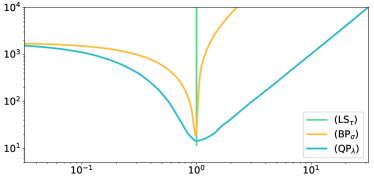
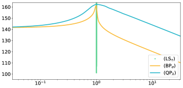
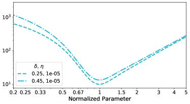
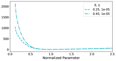
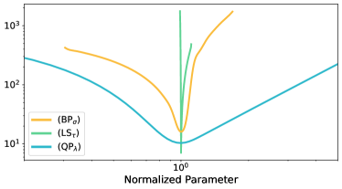
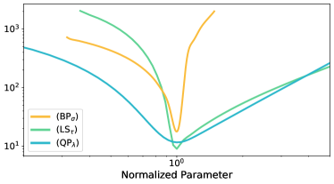
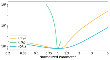
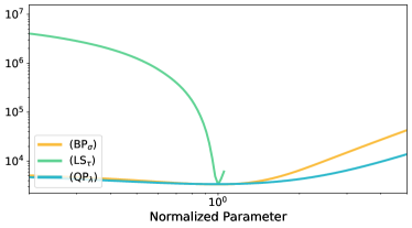
The numerics for $(\mathrm{LS}_{\tau})$, appearing in Figure 1, concern the case in which $\eta$ is small. When the ambient dimension is modest ($N=10^{4}$) and the noise scale only moderately small ($\eta=2\cdot 10^{-3}$), parameter instability of $(\mathrm{LS}_{\tau})$ is readily observed. Minute changes in $\tau$ lead to blow-up in the nnse and the peak signal-to-noise ratio (psnr) (left and right plot, respectively). Indeed, for the range plotted, it is difficult to visually segment the left half of the $(\mathrm{LS}_{\tau})$ average loss curve from the right half. These observations support the asymptotic theory of §V. Moreover, the simulations suggest that the other two programs, $(\mathrm{BP}_{\sigma})$ and $(\mathrm{QP}_{\lambda})$ are relatively much less sensitive to the choice of their governing parameter.

Figure 1: $(\mathrm{LS}_{\tau})$ parameter instability in the low-noise regime. Average loss (left) plotted on a log-log scale with respect to the normalized parameter; average psnr (right) plotted on a log-linear scale with respect to the normalized parameter. The data parameters are $(s,m,N,\eta,k,n)=(1,2500,10^{4},2\cdot 10^{-3},15,301)$.

VIII-B $(\mathrm{QP}_{\lambda})$ numerics

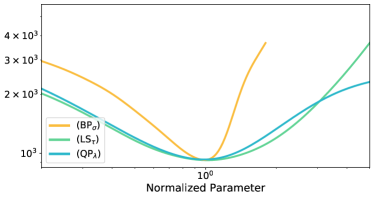
In this section we visualize the average loss of $(\mathrm{QP}_{\lambda})$ as a function of its normalized parameter $\rho=\lambda/\lambda^{*}$. In Figure 2, the average loss for $(\mathrm{QP}_{\lambda})$ is plotted with respect to the $\rho$ for an aspect ratio $\delta$ ranging between $0.25$ and $4$. As suggested by Theorem VI.1, the average loss appears to scale quadratically with respect to the normalized parameter for values $\rho>1$. For $\rho\in(0.5,0.9)$, the average loss appears to scale super-quadratically with respect to the normalized parameter, with the rate of growth increasing as a function of $\delta$. This behaviour suggests that $(\mathrm{QP}_{\lambda})$ can be sensitive to its parameter choice if $\rho$ is too small. The intuition for the observed behaviour is that $(\mathrm{QP}_{\lambda})$ increasingly behaves like ordinary least squares when $\lambda\to 0$. Each average loss was approximated from 15 realizations of the loss using multiquadric RBF interpolation. Due to concentration effects, the realizations for each parameter value clustered very closely to the approximated average loss. The left-hand plot Figure 2 is plotted on a log-log scale, while the right-hand plot is plotted on a linear-linear scale. The linear-linear plot readily demonstrates how over-guessing $\lambda$ by a factor of $2$ is more robust to error than under-guessing $\lambda$ by a factor of $2$.

Figure 2: Average loss of $(\mathrm{QP}_{\lambda})$ plotted with respect its normalized parameter in the low-noise, high sparsity regime. Parameters for the simulation are $(s,N,\eta,k,n)=(1,10^{4},10^{-5},15,301)$. The aspect ratio of the matrix $A\in\mathbb{R}^{m\times N}$ with $A_{ij}\overset{\text{iid}}{\sim}\mathcal{N}(0,m^{-1})$ takes values $\delta\in\{4^{-1},\ldots,4\}$, as shown in the legend. The data are visualized on a log-log scale (left) and linear scale (right).

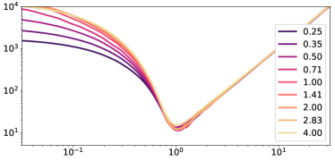
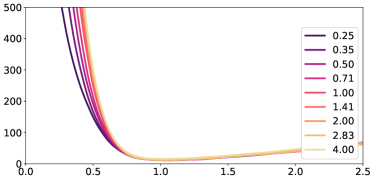
In Figure 3, we visualize $(\mathrm{QP}_{\lambda})$ average loss with respect to its normalized parameter. In the top row, we include two plots similar to Figure 2, but for $\delta=0.25,0.45$ only. Again, the left-hand plot is on a log-log scale while the right-hand plot is on a linear-linear scale. The bottom row depicts the goodness of fit of the RBF approximation for the average loss.

Figure 3: Average loss of $(\mathrm{QP}_{\lambda})$ plotted with respect to its normalized parameter in the low-noise, high-sparsity regime. Parameters for the simulation are $(s,N,\eta,k,n)=(1,10^{4},10^{-5},25,201)$. The aspect ratio of the matrix $A\in\mathbb{R}^{m\times N}$ with $A_{ij}\overset{\text{iid}}{\sim}\mathcal{N}(0,m^{-1})$ takes values $\delta=0.25,0.45$, as shown in the legend. The data in the top row are visualized on a $\log$-$\log$ scale (left) and linear scale (right). The bottom row depicts the quality of fit for the RBF approximation of the average loss for $\delta=0.25$ (left) and $\delta=0.45$ (right).

VIII-C $(\mathrm{BP}_{\sigma})$ numerics

This section includes numerical simulations depicting the sensitivity of $(\mathrm{BP}_{\sigma})$ to its parameter choice. These numerics serve to support the asymptotic theory developed in §VII.

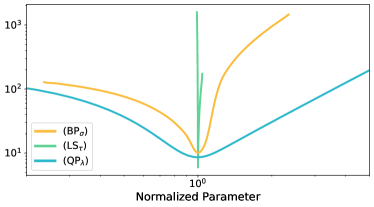
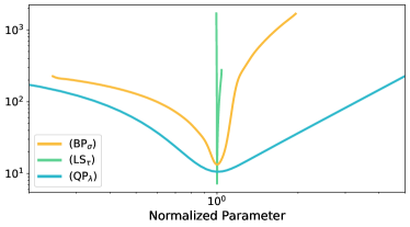
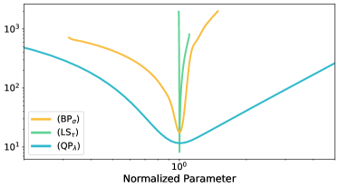
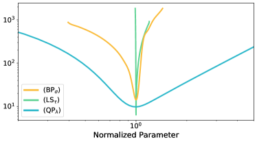
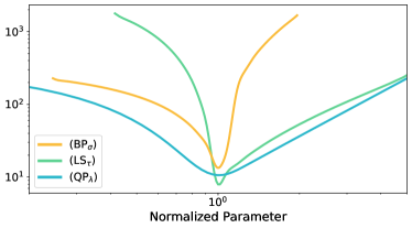
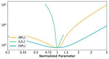
The graphics in Figure 4 serve as an initial depiction of $(\mathrm{BP}_{\sigma})$ parameter instability, depicting the average loss for each program and for $N\in\{4000,7000\}$, $\delta\in\{0.1,0.25,0.45\}$. Each plot depicts the average loss as a function of the normalized parameter for $(\mathrm{LS}_{\tau})$ (green), $(\mathrm{BP}_{\sigma})$ (orange) and $(\mathrm{QP}_{\lambda})$ (blue). The domain of the normalized parameter in each plot is $(0.2,5)$. A single realization of $A$ was fixed and the average loss was computed from $k=50$ realizations of the noise by constructing a function approximator using radial basis function approximation with a multiquadric kernel. The RBF approximator was evaluated on a logarithmically spaced grid of $n_{\text{rbf}}=301$ points centered about $1$. The loss values for $(\mathrm{LS}_{\tau})$ and $(\mathrm{BP}_{\sigma})$ were computed by using the program equivalence described by §II. In particular, for computational expediency, once $A$ and $z$ were fixed, the Lasso program was solved only using $(\mathrm{QP}_{\lambda})$, for all $\lambda$ in a specified range. For each $x^{\sharp}(\lambda)$, we obtained $\hat{x}(\tau)$ and $\tilde{x}(\sigma)$ using that $\hat{x}(\tau)=\tilde{x}(\sigma)=x^{\sharp}(\lambda)$ for $\tau:=\|x^{\sharp}(\lambda)\|_{1}$ and $\sigma:=\|y-Ax^{\sharp}(\lambda)\|_{2}$.

For convenience, we refer to each plot in Figure 4 via its (row, column) position in the figure. The collection of plots serves to depict how the average loss changes as a function of $N$ and $\delta=m/N$ when $\eta=1$. Namely, as $N$ increases, the average loss for $(\mathrm{BP}_{\sigma})$ becomes sharper about the optimal parameter choice. In addition, as $\delta$ increase, we observe the same phenomenon. In Figure 6, similar content is depicted, but for $\eta=100$. In this case, $n_{\text{rbf}}=501$ was used.

Specific paramter settings for the RBF approximation for each set of problem parameters and program are detailed in Table III. Because $(\mathrm{BP}_{\sigma})$ parameter instability is not easily visualized in small dimensions (e.g., for $N<10^{6}$), we supply several plots visualizing the quality of the RBF approximation. Namely, approximation quality plots corresponding with Figure 4 may be found in Figure 5; and approximation quality plots are included in Figure 6. Each row of these plots is a triptych; each column corresponds to a program: $(\mathrm{LS}_{\tau})$ for the left-most, $(\mathrm{BP}_{\sigma})$ in the centre; and $(\mathrm{QP}_{\lambda})$ on the right. These plots depict a single line and a collection of points. The points correspond to individual loss values for each realization of the noise and each normalize parameter value computed. The line corresponds to the RBF approximation of the average loss for that program. The domain for the $(\mathrm{LS}_{\tau})$ plots is $(0.95,0.95^{-1})$ in the normalized parameter space. For $(\mathrm{BP}_{\sigma})$ it is $(0.9,0.9^{-1})$, and for $(\mathrm{QP}_{\lambda})$ $(0.75,0.75^{-1})$.

In Figure 5, one may observe by inspection that the loss realizations for $(\mathrm{LS}_{\tau})$ and $(\mathrm{QP}_{\lambda})$ typically are achieved very close to $1$. In contrast, there is a relatively wider range in the domain for where the $(\mathrm{BP}_{\sigma})$ loss achieves its optimum. This is integral to how $(\mathrm{BP}_{\sigma})$ risk is sensitive to the choice of $\sigma$.

There appear to be two competing factors that impact sensitivity to parameter choice and program optimality. The first is stability of the parameter with respect to variation due to the noise realization. This has already been described: because $\sigma(\lambda^{*},z)$ varies greatly as a function of $z$, program optimality is destroyed by suboptimal loss values near $\sigma=\sigma^{*}$. On the other hand, this also tends to have somewhat of a smooth effect about the optimal normalized parameter. Thus, as $\tau(\lambda^{*},z)$ does not vary as greatly in this manner, its sensitivity to parameter choice is not smoothed due to local averaging effects.

a

Figure 4: Each plot depicts the average loss as a function of the normalized parameter for each of the three programs under consideration. The collection of plots depicts how the average loss changes as a function of $N$ and $\delta=m/N$. Details for each plot will be given by referencing the (row, column) position of the plot in this figure. The domain of the normalized parameter in each plot is $(0.2,5)$. A single realization of $A$ was fixed and the average loss was computed from $k=50$ realizations of the noise by constructing a function approximator using radial basis function approximation with a multiquadric kernel. The RBF approximator was evaluated on a logarithmically spaced grid of $n=301$ points centered about $1$. (1,1): $(s,N,\delta,\eta)=(1,4000,0.1,1)$; (1,2): $(s,N,\delta,\eta)=(1,7000,0.1,1)$; (2,1): $(s,N,\delta,\eta)=(1,4000,0.25,1)$; (2,2): $(s,N,\delta,\eta)=(1,7000,0.25,1)$; (3,1): $(s,N,\delta,\eta)=(1,4000,0.45,1)$.

$N=4000,\eta=1$ $N=7000,\eta=1$

a

Figure 5: Each plot depicts the quality of the RBF approximation about the optimal normalized parmaeter. The left-most plot is in every case depicting the loss and (approximate) average loss of $(\mathrm{LS}_{\tau})$; the middle that for $(\mathrm{BP}_{\sigma})$; and the right that for $(\mathrm{QP}_{\lambda})$. Top-to-bottom:$(s,N,\delta,\eta)=(1,4000,0.1,1)$; $(s,N,\delta,\eta)=(1,4000,0.25,1)$; $(s,N,\delta,\eta)=(1,4000,0.45,1)$; $(s,N,\delta,\eta)=(1,7000,0.1,1)$; $(s,N,\delta,\eta)=(1,7000,0.25,1)$.

   

Figure 6: Top row: Each plot depicts the average loss as a function of the normalized parameter for each of the three programs under consideration. The collection of plots depicts how the average loss changes as a function of $\delta=m/N$. The domain of the normalized parameter in each plot is $(0.2,5)$. A single realization of $A$ was fixed and the average loss was computed from $k=50$ realizations of the noise by constructing a function approximator using radial basis function approximation with a multiquadric kernel. The RBF approximator was evaluated on a logarithmically spaced grid of $n_{\text{rbf}}=501$ points centered about $1$. Bottom row: Each plot depicts the quality of the RBF approximation about the optimal normalized parmaeter. In each triptych, the left plot depicts the loss and (approximate) average loss of $(\mathrm{LS}_{\tau})$; the middle that for $(\mathrm{BP}_{\sigma})$; and the right that for $(\mathrm{QP}_{\lambda})$. Left column: $(s,N,\delta,\eta)=(1,7000,0.1,100)$; Right column: $(s,N,\delta,\eta)=(1,7000,0.25,100)$.

VIII-D More synthetic examples

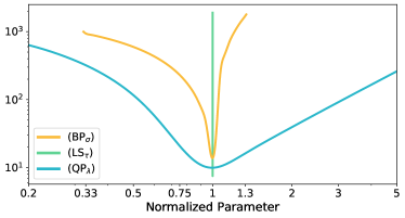
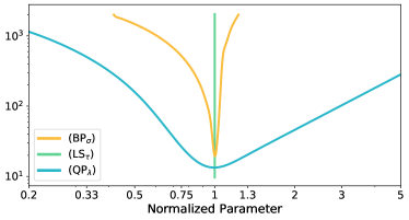
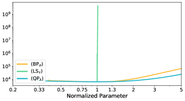
In this section, we display three synthetic examples where only $s$ and $\eta$ were changed. Thus, the effect of sparsity and noise scale is readily observed. In each of these figures, the aspect ratio of the measurement matrix was $\delta=0.25,0.45$ for the left- and right-hand plots respectively (except Figure 8 where $\delta=0.25$ was too small to achieve recovery). The average loss curves for each program were computed from $k=25$ realizations of loss curves that were, themselves, generated on a logarthmically spaced grid of $n=201$ points centered about the optimal choice of the normalized parameter, $\rho=1$. The loss realizations were again computed by solving $(\mathrm{QP}_{\lambda})$ and using the correspondence between Lasso programs to compute the loss curves for $(\mathrm{LS}_{\tau})$ and $(\mathrm{BP}_{\sigma})$.

The bottom row of Figure 7 and Figure 9, and the right half of Figure 8 depict the quality of the approximation of the average loss curve for each program. Specifically, each program appears with its own facet, in which are displayed the individual loss realizations $L(\rho_{i};x_{0},A,\eta z_{j}),i\in[n],j\in[k]$ as grey points, and the average loss $\bar{L}(\rho;x_{0},A,\eta)$ as a coloured line. The top row of Figure 7 and Figure 9, and the left half of Figure 8 compare the the average loss curves for each program, where the average losses are plotted on a log-log scale with respect to the normalized parameter.

The first figure, Figure 7, displays a setting similar to Figure 1. The noise scale was $\eta=10^{-5}$ and $s=1$. Thus, the setting depicts the low-noise high-sparsity regime. The second figure, Figure 8, depicts a moderately low-noise regime, with a large value of $s$ (so large that $\delta=0.25$ did not yield adequate recovery). Thus, this figure depicts the regime in which $x_{0}$ is near the limit of acceptable sparsity for the CS regime. Finally, the parameter settings for Figure 9 were $s=100$ and $\eta=100$. In particular, sparsity is modest, and the noise scale is large (the variance equals the ambient dimension, $\eta^{2}=N=10^{4}$).

It is readily observed that $(\mathrm{LS}_{\tau})$ is highly sensitive to its parameter choice in both low-noise regimes. We observe that $(\mathrm{BP}_{\sigma})$ becomes more sensitive to its parameter choice as sparsity decreases from $750$ to $100$ to $1$. Finally, we observe that $(\mathrm{QP}_{\lambda})$ is most sensitive to its parameter choice in the low-noise high-sparsity regime. This left-sided sensitivity is consistent with the theory and numerical simulations for the corresponding proximal denoising setting in [21, 20].

Figure 7: Parameter instability numerics in the low-noise, high-sparsity regime. Top row: Average loss is plotted with respect to the normalized parameter for each program. Bottom row: Visualizations of RBF approximation quality for average loss (best seen on a computer). Left: $(s,N,m,\eta,k,n)=(1,10^{4},2500,10^{-5},25,201)$; Right: $(s,N,m,\eta,k,n)=(1,10^{4},4500,10^{-5},25,201)$.

Figure 8: Parameter instability numerics in the low-sparsity regime with parameters $(s,N,m,\eta,k,n)=(750,10^{4},4500,10^{-1},25,201)$. Left: Average loss is plotted with respect to the normalized parameter for each program. Right: Visualizations of the RBF approximation quality for average loss.

Figure 9: Parameter instability numerics for intermediate parameter values: $(s,N,\eta,k,n)=(10^{2},10^{4},10^{-1},25,201)$. Left: $m=2500$; Right: $m=4500$. Top: Average loss is plotted with respect to the normalized parameter for each program. Bottom: Visualizations of average loss approximation quality.

VIII-E Realistic Examples

We next include two realistic examples in addition to the synethetic ones of the previous sections. We show how CS programs may exhibit sensitivity as a function of their governing parameter for a 1D and 2D wavelet problem. In each example, we will include plots similar to those appearing above; however there will be some key differences. As above, the average loss is computed from several realizations of the loss, which depend in turn on realizations of the noise. However, we will plot the loss corresponding to a single realization as a function of the normalized parameter. Computing the normalized parameter is what requires computing the average loss. As before, we approximate the average loss and the normalized parameter using RBF interpolation, described in §A-B1. The figures of this section contain three main pieces. We will plot psnr, as a function of the normalized parameter; loss, equal to the nnse, as a function of the normalized parameter; and we will include a grid of plots that allows for comparison of CS recovery by visualizing the recovery in the signal domain. The latter grid of plots shall be referred to as “grid plots” while the psnr and nnse plots shall be referred to as “reference plots”, as they contain annotations that relate them to the grid plots.

We now include a brief description of the so-called grid plots and associated reference plots that appear in this section. Other than plotting loss, rather than average loss, a key difference of the reference plots to the plots of §VIII-A–VIII-C is that they have been annotated with vertical black dashed lines, and coloured dots. Where the loss for a program intersects the black dashed line, we show a representative solution for that program where the normalized parameter for the problem is given by the x intercept of the vertical line (approximately). Because the programs were solved on a grid, the true value of the normalized program is given by the coloured dot appearing nearest the black dashed line. The $x$ axis for the reference plots is the normalized parameter (plotted on a log scale). The $y$ axis for the reference plots is either the psnr (plotted on a linear scale) or the nnse (plotted on a log scale). The representatives for each chosen normalized parameter value and each program are plotted as a faceted grid below the reference plot. The chosen normalized parameter value is given at the top of each column, while the program used to recover the noisy ground truth signal is described in the legend.

VIII-E1 1D wavelet compressed sensing

The signal $\xi_{0}\in\mathbb{R}^{N}$, $N=4096$, was constructed in the Haar-wavelet domain. In particular, $x_{0}\in\mathbb{R}^{N}$ has $10$ non-zero coefficients, each equal to $N$. Let $\mathcal{W}_{1}$ denote the $1$D Haar wavelet transform. Thus, $\xi_{0}=\mathcal{W}_{1}x_{0}$ where $\|x_{0}\|_{0}=10$. Next, for $A\in\mathbb{R}^{m\times N}$ where $m=1843$, define $y=Ax_{0}+\eta z$ where $z_{i}\overset{\text{iid}}{\sim}\mathcal{N}(0,1)$ and $\eta=50$. The signal’s wavelet coefficients were recovered using $(\mathrm{LS}_{\tau})$, $(\mathrm{QP}_{\lambda})$ and $(\mathrm{BP}_{\sigma})$ for several realizations of the noise $z$ and over a grid of normalized parameter values. For example $\hat{x}(\tau_{i};x_{0},A,z^{(j)})$ is the $(\mathrm{LS}_{\tau})$ recovery of the wavelet coefficients $x_{0}$ from $(y^{(j)},A)$ with $\tau=\tau_{i}$, where $y^{(j)}:=Ax_{0}+\eta z^{(j)}$. The recovered signal is thus given by $\hat{\xi}(\tau_{i}):=\mathcal{W}^{-1}\hat{x}(\tau_{i})$ and the loss given by $\eta^{-2}\|\hat{\xi}(\tau_{i})-\xi_{0}\|_{2}^{2}$. The loss modified similarly for the other programs. Specifically, the loss is measured in the signal domain and not the wavelet domain. The average loss was approximated from $k=50$ loss realizations using RBF interpolation, as described in §A-B1, on a grid of $n=501$ points logarithmically spaced and centered about $\rho=1$.

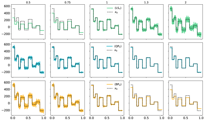
Results of this simulation are depicted in Figure 10 with RBF interpolation parameter settings given in Table IV. The results shown in Figure 10 depict data from only a single noise realization: the top-most graphic shows psnr as a function of the normalized parameter; the middle graphic plots the loss as a function of the normalized parameter; and the bottom group compares the ground-truth signal and recovered signals in the signal domain. While psnr and loss are plotted instead of average psnr and average loss, the normalized parameter was computed from the average loss, as usual (cf. §A-B1). Correspondingly, observe that the optimal parameter choice for each program may not appear at $\rho=1$, since the optimal normalized parameter for a particular loss realization is not necessarily equal to the optimal normalized parameter for the expected loss. In the bottom group of 15 plots, each row corresponds with a particular program — $(\mathrm{LS}_{\tau})$, $(\mathrm{QP}_{\lambda})$ and $(\mathrm{BP}_{\sigma})$, from top to bottom — while each column corresponds with a particular vaue of the normalized parameter — 0.5, 0.75, 1, 1.3 and 2, from left to right. The recovered signal for that program and normalized parameter value is shown as a coloured line, while the ground truth signal is shown as a black line.

As $\eta=50$, the problem lies outside of the small-noise regime. As such, $(\mathrm{BP}_{\sigma})$ is more sensitive to its parameter choice than $(\mathrm{QP}_{\lambda})$, and more sensitive than $(\mathrm{LS}_{\tau})$ for $\rho>1$ due to the relatively high sparsity of the signal. Since suboptimality of $(\mathrm{BP}_{\sigma})$ is observed for risk or average loss rather than for individual loss realizations, we do not observe suboptimality of $(\mathrm{BP}_{\sigma})$ loss in these graphics. As expected, $(\mathrm{LS}_{\tau})$ is sensitive to its parameter choice for $\rho<1$, as the ground-truth solution lies outside the feasible set in this setting. It appears that the loss is mildly more sensitive to under-guessing $\tau$ in this regime, than it is to over-guessing $\sigma$. This is readily observed from all of the plots in the figure, especially by comparing those in the bottom group of 15.

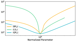
For comparison with the middle plot of Figure 10, we include a plot of the average loss for each program as a function of the normalized parameter in Figure 11 (left plot). Beside it is a triptych visualizing the RBF approximation quality for the average loss.

Figure 10: Realistic Example in 1D for $(s,N,m,\eta,k,n)=(10,4096,1843,50,50,501)$. Ground truth signal $x_{0}$ defined in the Haar wavelet domain with first $s$ coefficients equal to $N$. Noise added in the Haar wavelet domain; recovery error measured in the signal domain. Top: Average psnr as a function of the normalized parmaeter for each parameter. Middle: Average nnse as a function of the normalized parmaeter for each parameter. Bottom: The ground truth and recovered signal for a single realization of the noise, faceted by the approximate normalized parameter value (given in the title) and by program (as depicted in the legend).

Figure 11: Parameter sensitivity numerics for $1$D wavelet CS example with parameter settings $(s,N,m,\eta,kn)=(10,4096,1843,50,50,501)$. Left: Average loss for each program plotted with respect to the normalized parameter. Right: A visualization of approximation quality for the average loss: $(\mathrm{LS}_{\tau})$, $(\mathrm{BP}_{\sigma})$ and $(\mathrm{QP}_{\lambda})$, from left to right.

VIII-E2 2D Wavelet Compressed Sensing

Figure 12: The square Shepp-Logan phantom (sslp).

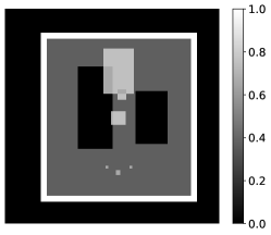
In this section, we describe numerical simulations for a 2D wavelet compressed sensing problem. The signal, $\xi_{0}$, is an $80\times 80$ image of the so-called square Shepp-Logan phantom (sslp), visualized in Figure 12. The sslp was first used in [20]. Let $\mathcal{W}$ denote the Haar wavelet transform and define $x_{0}:=\mathcal{W}\xi_{0}\in\mathbb{R}^{6400}$ to be the vector of Haar wavelet coefficients for the signal $\xi_{0}$. The linear measurements are taken as

$$y=Ax_{0}+\eta z,\qquad A_{ij}\overset{\text{iid}}{\sim}\mathcal{N}\left(0,m^{-1}\right),z_{i}\overset{\text{iid}}{\sim}\mathcal{N}(0,1),\eta>0.$$

The signal’s wavelet coefficients were recovered using $(\mathrm{QP}_{\lambda})$ to obtain $x^{\sharp}(\lambda_{i})$, where $i\in[n]$ enumerates the grid of parameter values. The recovered image is then given by $\xi^{\sharp}(\lambda_{i}):=\mathcal{W}^{-1}(x^{\sharp}(\lambda_{i}))$. By using the method described previously at the beginning of §VIII, the corresponding solutions for $(\mathrm{LS}_{\tau})$ and $(\mathrm{BP}_{\sigma})$ were computed, obtaining $\hat{x}(\tau_{i})$ and $\tilde{x}(\sigma_{i})$, respectively, in addition to the corresponding images $\hat{\xi}(\tau_{i}):=\mathcal{W}^{-1}(\hat{x}(\tau_{i}))$ and $\tilde{\xi}(\sigma_{i}):=\mathcal{W}^{-1}(\tilde{x}(\sigma_{i}))$, $i\in[n]$. As in §VIII-E1, the loss has been modified to measure the nnse in the image domain. For example, the $(\mathrm{LS}_{\tau})$ loss is given as $\eta^{-2}\|\hat{\xi}(\tau_{i})-\xi_{0}\|_{2}^{2}$; similarly for the other two programs.

Average loss as a function of the normalized parameter $\rho$ is shown in Figure 13 for $\eta=10^{-2},1/2$ with $m=2888$ (i.e., $m/N\approx 0.45$). The average loss was approximated using RBF interpolation from $k=50$ realizations along a logarithmically spaced grid of $501$ points centered about $\rho=1$ using the method described in §A-B1. The parameter settings for the RBF interpolation are provided in Table V. Plots showing the approximation quality of the RBF interpolation quality are given in the bottom row of Figure 13. In these plots, individual realizations of the nnse for the recovery are shown as grey points. The RBF interpolant is given by the coloured line in each plot. The approximation quality is only visualized for a narrow region about $\rho=1$. Indeed, the approximation quality of the RBF interpolant was observed, in every case, to be better away from $\rho=1$ than about $\rho=1$: ensuring good interpolation of the loss realizations about $\rho=1$ was observed to be sufficient for ensuring good interpolation of the average loss over the region of interest, $\rho\in[10^{-1},10^{1}]$.

In the left column of the figure, where $\eta=10^{-2}$, we observe that $(\mathrm{LS}_{\tau})$ is relatively more sensitive to its parameter choice than either $(\mathrm{BP}_{\sigma})$ or $(\mathrm{QP}_{\lambda})$. In particular, for this problem, we observe that $\eta=10^{-2}$ is sufficient to lie within the low-noise regime. Due to how the solutions for $(\mathrm{LS}_{\tau})$ were computed from those for $(\mathrm{QP}_{\lambda})$, the average loss curve for $(\mathrm{LS}_{\tau})$ is not resolved over the full domain for the normalized parameter. This reinforces how small changes in the normalized parameter value for $(\mathrm{LS}_{\tau})$ correspond to relatively much larger changes in the normalized parameter value for $(\mathrm{QP}_{\lambda})$.

In the right column of the figure, where $\eta=1/2$, we observe that $(\mathrm{BP}_{\sigma})$ is relatively more sensitive to its parameter choice than either $(\mathrm{LS}_{\tau})$ or $(\mathrm{QP}_{\lambda})$. We expect this is due to the relatively high sparsity of the signal. Again, the average loss curve for $(\mathrm{BP}_{\sigma})$ is not resolved over the full plotted domain of the normalized parameter. This underscores how changes in the governing parmeter for $(\mathrm{QP}_{\lambda})$ correspond with relatively smaller changes in the governing parameter for $(\mathrm{BP}_{\sigma})$. In particular $(\mathrm{BP}_{\sigma})$ is more sensitive to its governing parameter than $(\mathrm{QP}_{\lambda})$ in the present problem. This observation is supported by the theory of §VII-B.

As in previous numerical simulations, the bottom row of Figure 13 includes triptyches depicting the average loss approximation quality for the RBF interpolation of the loss realizations (cf. §A-B1).

   

Figure 13: Average loss for a 2D wavelet compressed sensing problem, plotted as a function of $\rho$; $(s,N,m)=(416,6418,2888)$ with $(k,n)=(50,501)$. Left: $\eta=10^{-2}$. Right: $\eta=1/2$. Top: The average loss (i.e., nnse) for each program as a function of $\rho$. The average loss was approximated using RBF interpolation with parameters given in Table V. Bottom: Plots to evaluate the quality of the RBF interpolation. In each polot, individual realizations of the loss are visible as grey points; the approximation to the average loss is visible as the coloured line through those points.

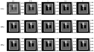
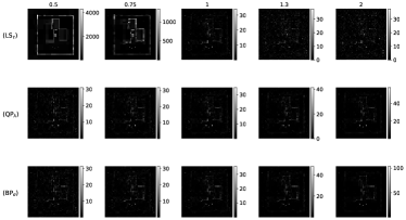
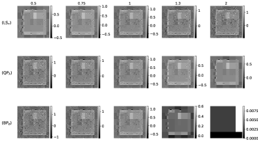
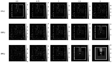
In both Figure 14 and Figure 15, we use four main elements to depict the results of a 2D wavelet CS problem, each for a single realization of the noise. In each figure, the top row depicts the psnr curves for each program (left) and loss curves for each program (right). The bottom row of the figure contains two groupings of the 15 plots each. Each grid of 15 plots is faceted by program ($(\mathrm{LS}_{\tau})$, $(\mathrm{BP}_{\sigma})$ and $(\mathrm{QP}_{\lambda})$, top-to-bottom) and normalized parameter value ($0.5$, $0.75$, $1$, $1.3$, $2$, left-to-right). Each (program, normalized parameter) tuple on the left-hand side of the figure corresponds with its partner on the right-hand side. Specifically, the left-hand grid of images depicts the recovered image for a given (program, normalized parameter) tuple, while the corresponding right-hand image depicts the pixel-wise nnse in the signal domain. The details of these images are best examined on a computer.

In Figure 14, the parameter settings are $(s,N,m,\eta,k,n)=(416,6418,2888,10^{-2},50,501)$. In particular, $\eta$ lies within the low-noise regime, as observed by the relative sensitivity of $(\mathrm{LS}_{\tau})$ to its parameter choice. In Figure 15, the parameter settings are $(s,N,m,\eta,k,n)=(416,6418,2888,1/2,50,501)$. In particular, the noise scale is relatively larger. The relatively high sparsity of the signal causes $(\mathrm{BP}_{\sigma})$ to be relatively more sensitive to its parameter choice than either $(\mathrm{LS}_{\tau})$ or $(\mathrm{QP}_{\lambda})$. These observations are supported by the theory of §V and §VII-B.

Figure 14: A 2D wavelet compressed sensing problem using the square Shepp-Logan phantom; $(s,N,m,\eta)=(416,6418,2888,10^{-2})$ with $(k,n)=(50,501)$. Top row: psnr (left) and nnse (right), plotted as a function of $\rho$. The plotted curves were generated from the single realization of the measurements that correspond to the grids depicted below them. Bottom grids: The left grid of 15 images shows the recovered image for each of five values of $\rho$: $\rho\in\{\frac{1}{2},\frac{3}{4},1,\frac{4}{3},2\}$; and for each program: $(\mathrm{LS}_{\tau})$, $(\mathrm{QP}_{\lambda})$, $(\mathrm{BP}_{\sigma})$. The right grid of 15 images shows the pixel-wise nnse of the recovered image for the same values of $\rho$, and for the three programs. Colour bars provide scale, and are best observed on a computer. The stated values of $\rho$ are approximate; the values of $\rho$ for which the images are depicted are marked by points in the nnse and psnr plots of the same colour as the loss curve on top of which they’re plotted.

Figure 15: A 2D wavelet compressed sensing problem using the square Shepp-Logan phantom; $(s,N,m,\eta)=(416,6418,2888,1/2)$ with $(k,n)=(50,501)$. Top row: psnr (left) and nnse (right), plotted as a function of $\rho$ for each program. The plotted curves were generated from the single realization of the measurements that correspond to the grids depicted below them. Bottom grids: The left grid of 15 images shows the recovered image for each of five values of $\rho$: $\rho\in\{\frac{1}{2},\frac{3}{4},1,\frac{4}{3},2\}$; and for each program: $(\mathrm{LS}_{\tau})$, $(\mathrm{QP}_{\lambda})$, $(\mathrm{BP}_{\sigma})$. The right grid of 15 images shows the pixel-wise nnse of the recovered image for the same values of the normalized parameter, and for the three programs. Colour bars provide scale, and are best observed on a computer. The stated values of $\rho$ are approximate; the values of $\rho$ for which the images are depicted are marked by points in the nnse and psnr plots of the same colour as the loss curve on top of which they’re plotted.

IX Proofs

IX-A Risk equivalences

Proof of §II.

The left-most inequality,

$$cs\log(N/s)\leq M^{*}(s,N),$$

is a consequence of [40, Theorem 1], and the second inequality,

$$M^{*}(s,N)\leq\inf_{\lambda>0}\sup_{x_{0}\in\Sigma_{s}^{N}}R^{\sharp}(\lambda;x_{0},A,\eta)$$

is trivial. The third inequality,

$$\inf_{\lambda>0}\sup_{x_{0}\in\Sigma_{s}^{N}}R^{\sharp}(\lambda;x_{0},A,\eta)\leq C_{\delta}R^{*}(s,A)$$

is a consequence of [9, Theorem 6] and §IX-B. Indeed, $R^{*}(s,A)$ may be lower-bounded by the optimally tuned worst-case risk, $\sup_{x\in\Sigma_{s}^{N}}\hat{R}(\|x\|_{1};x,A,\eta)$, which is again lower-bounded by $cs\log(N/s)$ due to [40, Theorem 1]. In particular, selecting constants appropriately gives

$$\inf_{\lambda>0}\sup_{x_{0}\in\Sigma_{s}^{N}}R^{\sharp}(\lambda;x_{0},A,\eta)$$

$$\qquad\leq C_{\delta}s\log(N/s)\leq C_{\delta}M^{*}(s,N)$$

$$\qquad\leq C_{\delta}\sup_{x\in\Sigma_{s}^{N}}\hat{R}(\|x\|_{1};x,A,\eta)\leq C_{\delta}R^{*}(s,A).$$

The final inequality, a variant of which may be found in [19] or [15], easily follows from §IX-C3.

∎

IX-B $\hat{R}$ is nearly monotone

We first quote a specialized version of a result introduced in [19], which gives a kind of local characterization of the deviation inequality presented in Theorem IV.4.

Theorem IX.1 ([19, Theorem 1.7]).

Let $A$ be a normalized $K$-subgaussian matrix and $T\subseteq\mathbb{R}^{N}$ a convex set. For any $t\geq 1$, it holds with probability at least $1-\exp(-t^{2})$ that

$$\left|\|Ax\|_{2}-\sqrt{m}\|x\|_{2}\right|\leq t\cdot C\tilde{K}\gamma(T\cap\|x\|_{2}B_{2}^{N}),\qquad\text{for all }x\in T.$$

We now present the main result of this section.

Proposition ($\hat{R}$ is nearly monotone).

Let $A$ be a normalized $K$-subgaussian matrix and $\mathcal{K}\subseteq\mathbb{R}^{N}$ a non-empty closed convex set. Fix $\delta,\eta>0$, $0<\tau_{1}\leq\tau_{2}<\infty$ and $x_{0}\in\mathcal{K}$ with $\|x_{0}\|_{\mathcal{K}}=1$. For any $t\geq 1$, if $m$ satisfies $m>Ct^{2}\tilde{K}^{2}\delta^{-2}\gamma^{2}(T_{\mathcal{K}}(x_{0})\cap\mathbb{S}^{N-1})$, then with probability at least $1-\exp(-t^{2})$ on the realization of $A$,

$$\hat{R}(\tau_{1};\tau_{1}x_{0},A,\eta)\leq\frac{1+\delta}{1-\delta}\hat{R}(\tau_{2};\tau_{2}x_{0},A,\eta).$$

Proof of §IX-B.

Given $0<\tau_{1}\leq\tau_{2}<\infty$, let $\tau\in\{\tau_{1},\tau_{2}\}$, define $y(\tau)=A\tau x_{0}+\eta z$, and define

$$q(\tau):=A\hat{w}(\tau),\quad\text{where}\quad\hat{w}(\tau) :=\hat{x}(\tau;A,y)-\tau x_{0},$$

$$\tau \in\{\tau_{1},\tau_{2}\}.$$

Observe that $q(\tau)$ may be written as

$$q(\tau) \in\operatorname*{\arg\min}\{\|q-\eta z\|_{2}:q\in\tau\mathcal{K}^{\prime}\},$$

$$\mathcal{K}^{\prime} :=\{A(x-x_{0}):x\in\mathcal{K}\}.$$

The set $\mathcal{K}^{\prime}\subseteq\mathbb{R}^{m}$ is non-empty, closed and convex, with $0\in\mathcal{K}^{\prime}$. In particular, §IV-F implies

$$\|q(\tau_{1})\|_{2}\leq\|q(\tau_{2})\|_{2}.$$

By [19, Theorem 1.7], for any $t\geq 1$ it holds with probability at least $1-\exp(-t^{2})$ on $A$ that for all $w\in T_{\mathcal{K}}(x_{0})$,

$$\sqrt{m}\cdot\left|\|Aw\|_{2}-\|w\|_{2}\right|\leq Ct\tilde{K}\gamma(T_{\mathcal{K}}(x_{0})\cap\mathbb{S}^{N-1}).$$

Accordingly, since $\hat{w}(\tau)\in T_{\mathcal{K}}(x_{0})$ for $\tau=\tau_{1},\tau_{2}$, under the assumption on $m$ it holds with probability at least $1-\exp(-t^{2})$

$$(1-\delta)\|\hat{w}(\tau_{1})\|_{2} \leq\|q(\tau_{1})\|_{2}$$

$$\leq\|q(\tau_{2})\|_{2}\leq(1+\delta)\|\hat{w}(\tau_{2})\|_{2}.$$

In particular, $\|\hat{w}(\tau_{1})\|_{2}\leq\frac{1+\delta}{1-\delta}\|\hat{w}(\tau_{2})\|_{2}$. As $z$ was arbitrary, the result follows:

$$\hat{R}(\tau_{1},\tau_{1}x_{0},A,\eta)\leq\frac{1+\delta}{1-\delta}\hat{R}(\tau_{2};\tau_{2}x_{0},A,\eta).$$

∎

Corollary .

Under the assumptions of §IX-B, the optimally tuned worst-case risk for $(\mathrm{LS}_{\tau})$ is nearly equivalent to $R^{*}(s,A)$, in the sense that

$$R^{*}(s,A)\leq\sup_{x\in\Sigma_{s}^{N}}\hat{R}(\|x\|_{1};x,A,\eta)\leq CR^{*}(s,A).$$

Proof of §IX-B.

The $\sup$ defining the optimally tuned worst-case risk may be decoupled as

$$\sup_{x^{\prime}\in\Sigma_{s}^{N}}\hat{R}(\|x^{\prime}\|_{1};x^{\prime},A,\eta)=\sup_{\tau>0}\sup_{x\in\Sigma_{s}^{N}\cap\mathbb{S}^{N-1}}\hat{R}(\tau;\tau x,A,\eta).$$ (4)

Applying a standard scaling property gives the relation:

$$\hat{R}(\tau;\tau x,A,\eta) =\left(\frac{\tau}{\eta}\right)^{2}\operatorname{\mathbb{E}}\|\hat{x}(1;y/\tau,A)-x\|_{2}^{2}$$

$$=\hat{R}(1;x,A,\eta/\tau).$$

The lower bound follows trivially from these two observations. To prove the upper bound, we start by observing two facts. First, $\Sigma_{s}^{N}\cap\mathbb{S}^{N-1}$ is compact, so there is $x^{*}(\tau)$ achieving the supremum over the set $\Sigma_{s}^{N}\cap\mathbb{S}^{N-1}$ in (4). Next, if the supremum over $\tau>0$ is achieved for $\tau\to\infty$, there is nothing to show, since

$$\sup_{\tau>0} \sup_{x\in\Sigma_{s}^{N}\cap\mathbb{S}^{N-1}}\hat{R}(\tau;\tau x,A,\eta)$$

$$=\lim_{\tau\to\infty}\sup_{x\in\Sigma_{s}^{N}\cap\mathbb{S}^{N-1}}\hat{R}(\tau;\tau x,A,\eta)$$

$$=\lim_{\tau\to\infty}\sup_{x\in\Sigma_{s}^{N}\cap\partial B_{1}^{N}}\hat{R}(1;x,A,\eta/\tau)$$

$$=\lim_{\eta\to 0}\sup_{x\in\Sigma_{s}^{N}\cap\partial B_{1}^{N}}\hat{R}(1;x,A,\eta).$$

Otherwise, the supremum is achieved for some $0\leq\tau^{*}<\infty$. Let $(\tau_{i})_{i\in\mathbb{Z}}$ be an arbitrary bi-infinite monotone sequence with $\tau_{i}\xrightarrow{i\to-\infty}\tau^{*}$ and $\tau_{i}\xrightarrow{i\to\infty}\infty$. For any $i\leq j$, §IX-B and properties of the supremum give

$$\sup_{x\in\Sigma_{s}^{N}\cap\mathbb{S}^{N-1}} \hat{R}(\tau_{i};\tau_{i}x,A,\eta)$$

$$=\hat{R}(\tau_{i};\tau_{i}x^{*}(\tau_{i}),A,\eta)$$

$$\leq C\hat{R}(\tau_{j};\tau_{j}x^{*}(\tau_{i}),A,\eta)$$

$$\leq C\hat{R}(\tau_{j};\tau_{j}x^{*}(\tau_{j}),A,\eta)$$

$$=C\sup_{x\in\Sigma_{s}^{N}\cap\mathbb{S}^{N-1}}\hat{R}(\tau_{j};\tau_{j}x,A,\eta)$$

As the above chain of inequalities holds for any pair $i<0$ and $j>0$, taking $i\to-\infty$ and $j\to\infty$ gives,

$$\sup_{\tau>0}\sup_{x\in\Sigma_{s}^{N}\cap\mathbb{S}^{N-1}}\hat{R}(\tau;\tau x,A,\eta) \leq C\sup_{x\in\Sigma_{s}^{N}\cap\mathbb{S}^{N-1}}\hat{R}(\tau_{j};\tau_{j}x,A,\eta)$$

$$\xrightarrow{j\to\infty}C\liminf_{\tau\to\infty}\sup_{x\in\Sigma_{s}^{N}\cap\mathbb{S}^{N-1}}\hat{R}(\tau;\tau x,A,\eta).$$

Finally, combining the above with an application of the standard scaling property yields

$$\sup_{\tau>0} \sup_{x\in\Sigma_{s}^{N}\cap\mathbb{S}^{N-1}}\hat{R}(\tau;\tau x,A,\eta)$$

$$\leq C\liminf_{\tau\to\infty}\sup_{x\in\Sigma_{s}^{N}\cap\mathbb{S}^{N-1}}\hat{R}(\tau;\tau x,A,\eta)$$

$$=C\liminf_{\tau\to\infty}\sup_{x\in\Sigma_{s}^{N}\cap\partial B_{1}^{N}}\hat{R}(1;x,A,\eta/\tau)$$

$$=C\liminf_{\eta\to 0}\sup_{x\in\Sigma_{s}^{N}\cap\partial B_{1}^{N}}\hat{R}(1;x,A,\eta)$$

∎

IX-B1 Controlling a conditionally Gaussian process

Here we ready two technical results that are used to control the error of the tuned approximation ($\tau=\tau^{*}$) uniformly with respect to the noise scale $\eta>0$. First, we specialize a result of [19]. Next, with high probability we control in expectation the extreme values of a conditionally Gaussian process.

Lemma (Corollary of Theorem IV.4).

Fix $\delta,\varepsilon,r>0$ and let $A\in\mathbb{R}^{m\times N}$ be a normalized $K$-subgaussian matrix. For a constant $C_{\varepsilon}>0$, if

$$m>C_{\varepsilon}\delta^{-2}\tilde{K}^{2}r^{2}s\log\left(\frac{2N}{s}\right),$$ (5)

it holds with probability at least $1-\varepsilon$ on the realization of $A$ that

$$\sup_{x\in\mathcal{L}_{s}(r)}\left|\|Ax\|_{2}-\|x\|_{2}\right|<\delta.$$ (6)

Proof of §IX-B1.

If $s=0$ the result holds trivially. For $s\geq 1$, this lemma is a straightforward consequence of Theorem IV.4. Set $u:=\sqrt{\log(2\varepsilon^{-1})}$. Indeed, by that result, it holds with probability at least $1-\varepsilon$ on the realization of $A$ that

$$\sup_{x\in\mathcal{L}_{s}(r)} \left|\|Ax\|_{2}-\|x\|_{2}\right|$$

$$\leq C_{1}m^{-1/2}\tilde{K}r\left[\operatorname{w}(\Sigma_{s}^{N}\cap\mathbb{S}^{N-1})+u\right],$$

where $C_{1}$ is an absolute constant. By §IV-D, there is an absolute constant $C_{2}>0$ so that

$$\operatorname{w}^{2}(\Sigma_{s}^{N}\cap\mathbb{S}^{N-1})\leq C_{2}^{2}s\log\left(\frac{2N}{s}\right).$$

In particular, (6) holds if

$$C_{1}\tilde{K}m^{-1/2}r\left[C_{2}\sqrt{s\log\left(\frac{2N}{s}\right)}+u\right]<\delta.$$

Observe that this condition is satisfied if (5) holds:

$$m >C_{\varepsilon}\delta^{-2}\tilde{K}^{2}r^{2}s\log\left(\frac{2N}{s}\right),$$

$$C_{\varepsilon} :=4C_{1}^{2}\cdot\max\left\{\log\left(2\varepsilon^{-1}\right),C_{2}^{2}\right\}.$$

∎

Lemma (Conditionally Gaussian process).

Let $\mathcal{K}\subseteq\mathcal{K}_{s}^{N}\cap\mathbb{S}^{N-1}$ and suppose $A\in\mathbb{R}^{m\times N}$ is a normalized $K$-subgaussian matrix. Let $z\in\mathbb{R}^{m}$ with $z_{i}\overset{\text{iid}}{\sim}\mathcal{N}(0,1)$ and define

$$f(A,z):=\sup_{x\in\mathcal{K}}\langle Ax,z\rangle.$$

Let $\delta,\varepsilon>0$ and $s\in\mathbb{N}$ with $s\geq 1$. There is an absolute constant $C_{\varepsilon}>0$, depending only on $\varepsilon$, so that if

$$m>C_{\varepsilon}\delta^{-2}\tilde{K}^{2}s\log(N/s),$$

then with probability at least $1-\varepsilon$ on the realization of $A$,

$$\operatorname{\mathbb{E}}\left[f(A,z)\mid A\right]\leq C_{\delta}\sqrt{s\log(2N/s)}$$

where $C_{\delta}>0$ is an absolute constant depending only on $\delta$.

Proof of §IX-B1.

By §IV-D,

$$\mathcal{K}\subseteq\mathcal{K}_{s}^{N}\cap\mathbb{S}^{N-1}\subseteq\mathcal{L}_{s}.$$

Therefore, $f(A,z)\leq\sup_{x\in\mathcal{L}_{s}}\langle Ax,z\rangle$. Furthermore,

$$\mathcal{L}_{s}-\mathcal{L}_{s}\subseteq\mathcal{L}^{*}_{s}.$$

By §IX-B1,

$$\max_{j\in[N]}\left|\|A^{j}\|_{2}-1\right|\leq\sup_{x\in\mathcal{L}^{*}_{s}}\left|\|Ax\|_{2}-\|x\|_{2}\right|<\delta$$ (7)

with probability at least $1-\varepsilon$ if $m$ satisfies

$$m>32C_{\varepsilon}\delta^{-2}\tilde{K}^{2}s\log(N/s).$$ (8)

Next, where $x\in\mathcal{L}_{s}$, define the random processes

$$X_{x} :=\langle Ax,z\rangle, z_{i} \overset{\text{iid}}{\sim}\mathcal{N}(0,1);$$

$$Y_{x} :=(1+\delta)\langle x,g\rangle, g_{i} \overset{\text{iid}}{\sim}\mathcal{N}(0,1).$$

Assume (8) holds and condition on the event $\mathcal{A}$ described by (7). Then $x-y\in\mathcal{L}_{s}-\mathcal{L}_{s}\subseteq\mathcal{L}^{*}_{s}$, so

$$\operatorname{\mathbb{E}}(X_{y}-X_{x})^{2} =\|A(x-y)\|_{2}^{2}$$

$$\leq(1+\delta)^{2}\|x-y\|_{2}^{2}=\operatorname{\mathbb{E}}(Y_{y}-Y_{x})^{2}.$$

Namely, conditioned on $\mathcal{A}$, the Sudakov-Fernique inequality (Theorem IV.5) gives

$$\operatorname{\mathbb{E}}\left[f(A,z)\mid A\right] \leq\operatorname{\mathbb{E}}\left[\sup_{x\in\mathcal{L}_{s}}X_{x}\right]\leq\operatorname{\mathbb{E}}\left[\sup_{x\in\mathcal{L}_{s}}Y_{x}\right]$$

$$=(1+\delta)\operatorname{w}(\mathcal{L}_{s})$$

$$\leq 2C(1+\delta)\sqrt{s\log(2N/s)},$$

where $C>0$ is an absolute constant.

∎

Remark IX.1 (Subgaussianity of $f(A,z)\mid A$).

Conditioned on $A$, Borell-TIS (Theorem IV.2) gives subgaussian concentration of $f(A,z)$ about $\operatorname{\mathbb{E}}[f(A,z)\mid A]$. In particular,

$$\left\|f(A,z)-\operatorname{\mathbb{E}}\left[f(A,z)\mid A\right]\right\|_{\Psi_{2}}\lesssim\sigma_{\mathcal{K}}$$

where, on the event $\mathcal{A}$ as defined in the proof of §IX-B1,

$$\sigma_{\mathcal{K}}^{2}=\sup_{x\in\mathcal{K}}\operatorname{\mathbb{E}}\left[|\langle Ax,z\rangle|^{2}\right]=\sup_{x\in\mathcal{K}}\|Ax\|_{2}^{2}\leq(1+\delta)^{2}.$$

Note that subgaussianity of $f(A,z)$ about $\operatorname{\mathbb{E}}[f(A,z)\mid A]$ can also be established using concentration of Lipschitz functions of Gaussians. Indeed, since $\mathcal{K}\subseteq\mathbb{S}^{N-1}$, for each $A$ it holds that $f(A,z)$ is Lipschitz in $z$. In fact, one can show that “for most” $A$, $f(A,z)$ is “nearly” $1$-Lipschitz.

IX-C Proofs for constrained Lasso sensitivity

IX-C1 Suboptimal choice of $\tau$

The first result required to prove Theorem V.1 concerns the case where $(\mathrm{LS}_{\tau})$ is controlled by a parameter that is too large. Under mild regularity assumptions on the mapping $A$, we show that this underconstrained problem cannot recover even the least-squares proximal denoising error rate in the limiting low-noise regime. The second result of this section concerns the situation where $\tau$ is too small, $\tau<\tau^{*}$. In this overconstrained problem, the ground truth does not lie in the feasible set and one expects this to be detrimental to recovery performance. We confirm this intuition irrespective of the assumptions on the measurement matrix $A$.

Lemma (Underconstrained $(\mathrm{LS}_{\tau})$).

Let $A\in\mathbb{R}^{m\times N}$ and assume that $\dim(\operatorname{\mathrm{null}}(A))>0$. Given $x_{0}\in\mathbb{R}^{N},\eta>0$ and $z\in\mathbb{R}^{m}$ with $z_{i}\overset{\text{iid}}{\sim}\mathcal{N}(0,1)$, let $y:=Ax_{0}+\eta z$. Suppose $\tau>\|x_{0}\|_{1}$. Almost surely on the realization of $z$,

$$\lim_{\eta\to 0}\hat{L}(\tau;x_{0},A,\eta z)=\infty.$$

Proof of §IX-C1.

Define $\rho:=\tau-\tau^{*}$, where $\tau^{*}:=\|x_{0}\|_{1}$. For simplicity, first assume $\operatorname{\mathrm{span}}(A)=\mathbb{R}^{m}$. There exists $\zeta\in\mathbb{R}^{N}$ such that $A\zeta=z$, and so $A(x_{0}+\eta\zeta)=Ax_{0}+\eta z=y$. Moreover, if $\eta<\rho\|\zeta\|_{1}^{-1}$ then $x_{0}+\eta\zeta\in\tau B_{1}^{N}$. In particular, $\xi:=x_{0}+\eta\zeta$ solves $(\mathrm{LS}_{\tau})$, because it is feasible and achieves the lowest possible objective value for $(\mathrm{LS}_{\tau})$. Notice $\|\zeta\|_{1}<\infty$ almost surely, so for any realization of $z$, $\eta<\rho\|\zeta\|_{1}^{-1}$ holds for all $\eta$ sufficiently small. Specifically, we have constructed $\xi$ solving $(\mathrm{LS}_{\tau})$, and lying on the interior of $\tau B_{1}^{N}$. Consequently, almost surely there is $\nu\in\operatorname{\mathrm{null}}(A)$ so that $\xi+\nu\in\tau B_{1}^{N}$ and still $A(\xi+\nu)=y$. Scale $\nu$ if necessary so that $\|\xi+\nu\|_{1}\in[\frac{1}{2}(\tau+\tau_{*}),\tau]$. Then, almost surely on the realization of $z$,

$$\hat{L}(\tau;x_{0},A,\eta z) \geq\eta^{-2}\|\xi+\nu-x_{0}\|_{2}^{2}$$

$$\geq\frac{1}{N\eta^{2}}\|\xi+\nu-x_{0}\|_{1}^{2}$$

$$\geq\frac{\rho^{2}}{4N\eta^{2}}\xrightarrow{\eta\to 0}\infty.$$

The case $\operatorname{\mathrm{span}}(A)\neq\mathbb{R}^{m}$ is similar. This case is interesting only when $z\in\mathbb{R}^{m}\setminus\operatorname{\mathrm{span}}(A)\neq\emptyset$, otherwise we argue as above. In this setting, define $P$ to be the projection onto the range of $A$ with $P^{\perp}=(I-P)$ being its orthogonal component. We may re-write the objective of $(\mathrm{LS}_{\tau})$ as

$$\|y-Ax\|_{2}^{2} =\|(P+P^{\perp})(y-Ax)\|_{2}^{2}$$

$$=\|P(y-Ax)+P^{\perp}y\|_{2}^{2}$$

$$=\|\tilde{y}-Ax\|_{2}^{2}+\|P^{\perp}y\|_{2}^{2}$$

where $\tilde{y}:=Py$. Therefore, when $z\not\in\operatorname{\mathrm{span}}(A)$, solving $(\mathrm{LS}_{\tau})$ is equivalent to solving

$$\operatorname*{\arg\min}\left\{\|Py-Ax\|_{2}:\|x\|_{1}\leq\tau\right\}. \star$$ ()

By construction, $\tilde{y}=Py\in\operatorname{\mathrm{range}}(A)$, so we may apply the same argument as above to the program $(\star)$, implying

$$\lim_{\eta\to 0}\hat{L}(\tau;x_{0},A,\eta z)=\infty.$$

∎

Lemma (Overconstrained $(\mathrm{LS}_{\tau})$).

Fix $\tau<\tau^{*}$. Almost surely on the realization $z$,

$$\lim_{\eta\rightarrow 0}\hat{L}\left(\tau;x_{0},A,\eta z\right)=\infty.$$

Proof of §IX-C1.

Let $\rho:=\tau^{*}-\tau>0$. For any solution $\xi$ to $(\mathrm{LS}_{\tau})$, one has

$$\eta^{-2}\|\xi-x_{0}\|_{2}^{2}\geq\frac{\rho^{2}}{N\eta^{2}}.$$

By definition, the desired result follows immediately:

$$\lim_{\eta\to 0}\hat{L}(\tau;x_{0},A,\eta z)\geq\eta^{-2}\|\xi-x_{0}\|_{2}^{2}\geq\frac{\rho^{2}}{N\eta^{2}}\xrightarrow{\eta\to 0}\infty.$$

∎

IX-C2 Uniform control over noise scales

In this section, we control $(\mathrm{LS}_{\tau})$ in the optimally tuned setting, uniform over the noise scale $\eta$. Specifically, for any $x_{0}\in\Sigma_{s}^{N}$ we control the expected error of recovery for $(\mathrm{LS}_{\tau})$ uniformly over the noise scale $\eta>0$. The results of §IX-B1 are crucial for this purpose.

Proposition (Uniform over noise scale).

Let $0\leq s<N<\infty$ be integers and let $m\in\mathbb{N}$. Let $A\in\mathbb{R}^{m\times N}$ be a normalized $K$-subgaussian matrix, and fix $\delta,\varepsilon>0$. Suppose that $y=Ax_{0}+\eta z$ for $\eta>0$ and $z\in\mathbb{R}^{m}$ with $z_{i}\overset{\text{iid}}{\sim}\mathcal{N}(0,1)$. With probability at least $1-\varepsilon$ on the realization of $A$, there exist constants $C_{\delta},C_{\varepsilon}>0$ so that if

$$m>C_{\varepsilon}\delta^{-2}\tilde{K}^{2}s\log\left(\frac{N}{2s}\right),$$

then for all $\eta>0$:

$$\operatorname{\mathbb{E}}\left[\|\hat{x}-x_{0}\|_{2}^{2}\mid A\right] \leq C_{\delta}\eta^{2}s\log\left(\frac{N}{2s}\right).$$

where $\hat{x}=\hat{x}(\tau^{*})$ solves $(\mathrm{LS}_{\tau})$ with $\tau=\tau^{*}:=\|x_{0}\|_{1}$.

Proof of §IX-C2.

If $s=0$, the result holds trivially as, by construction, $\|\hat{x}-x_{0}\|_{2}=0$ almost surely. Suppose $s\geq 1$. By definition of $\hat{x}$, where $h:=\hat{x}-x_{0}$,

$$\|A\hat{x}-y\|_{2}^{2}\leq\|Ax_{0}-y\|_{2}^{2}\quad\implies\quad\|Ah\|_{2}^{2}\leq 2\eta\langle Ah,z\rangle.$$

Step 1: Lower bound $\|Ah\|_{2}$ with high probability. Note that $\|Aw\|_{2}=\|w\|_{2}\|A\hat{w}\|_{2}$ for $w\neq 0$ where $\hat{w}:=w/\|w\|_{2}$. By §IX-B1, there is an event $\mathcal{A}_{1}$ with $\mathbb{P}(\mathcal{A}_{1})\geq 1-\varepsilon/2$ on which

$$\sup_{x\in\mathcal{K}_{4s}^{N}}\left|\|Ax\|_{2}-\|x\|_{2}\right|\leq\sup_{x\in\mathcal{L}_{4s}}\left|\|Ax\|_{2}-\|x\|_{2}\right|<\delta_{1}$$

if $m$ satisfies

$$m>16C_{\varepsilon}^{\prime}\delta_{1}^{-2}\tilde{K}^{2}s\log\left(\frac{N}{2s}\right).$$ (9)

Specifically, $h\in\mathcal{J}_{4s}^{N}$ by §IV-D, meaning $\hat{h}\in\mathcal{J}_{4s}^{N}\cap\mathbb{S}^{N-1}\subseteq\mathcal{K}_{4s}^{N}$ if $h\neq 0$. So, conditioning on $\mathcal{A}_{1}$ and enforcing (9), one has

$$\|Ah\|_{2}^{2} =\|h\|_{2}^{2}\|A\hat{h}\|_{2}^{2}\geq\|h\|_{2}^{2}\left(\|\hat{h}\|_{2}-\delta_{1}\right)^{2}\geq(1-\delta_{1})^{2}\|h\|_{2}^{2}.$$ (10)

The inequality $(1-\delta_{1})^{2}\|h\|_{2}^{2}\leq\|Ah\|_{2}^{2}$ holds also for $h=0$.

Step 2a: Upper bound $\langle Ah,z\rangle$. Again using that $h\in\mathcal{J}_{4s}^{N}$,

$$2\eta\langle Ah,z\rangle\leq 2\eta\|h\|_{2}\sup_{\hat{h}\in\mathcal{K}_{4s}^{N}\cap\mathbb{S}^{N-1}}\langle A\hat{h},z\rangle.$$ (11)

Step 2b: Control the latter quantity in expectation. By §IX-B1, there is $C_{\varepsilon}^{\prime\prime}>0$ so that for

$$m>4C_{\varepsilon}^{\prime\prime}\delta^{-2}\tilde{K}^{2}s\log\left(\frac{N}{4s}\right),$$ (12)

there is an event $\mathcal{A}_{2}$ holding with probability at least $1-\varepsilon/2$, on which there is a constant $C_{\delta}>0$ such that

$$\operatorname{\mathbb{E}}\left[\sup_{\hat{h}\in\mathcal{K}_{4s}^{N}}\langle A\hat{h},z\rangle\mid A\right]\leq 2C_{\delta}\sqrt{s\log\left(\frac{N}{2s}\right)}.$$

Step 3: Now combine steps 1 and 2a. Assume $m$ simultaneously satisfies (9) and (12), and condition on $\mathcal{A}_{1}\cap\mathcal{A}_{2}$, which holds with probability at least $1-\varepsilon$. Combining (10) and (11), and letting $\delta_{1}:=1-2^{-1/2}$ gives

$$\|h\|_{2}\leq 4\eta\sup_{\hat{h}\in\mathcal{K}_{4s}^{N}}\langle A\hat{h},z\rangle.$$

Take expectation of both sides and bound the quantity by applying step 2b. This yields,

$$\operatorname{\mathbb{E}}\left[\|h\|_{2}\mid A\right]\leq 8C_{\delta}\eta\sqrt{s\log\left(\frac{N}{2s}\right)}.$$

Note that by setting $C_{\varepsilon}:=\max\{\frac{32C_{\varepsilon}^{\prime}}{3-2\sqrt{2}},4C_{\varepsilon}^{\prime\prime}\}$, it suffices to require

$$m>C_{\varepsilon}\delta^{-2}\tilde{K}^{2}s\log\left(\frac{N}{2s}\right).$$

Alternatively, one may also apply a standard fact for subgaussian random variables. Recall as in (1), ${\left|\kern-1.07639pt\left|\kern-1.07639pt\left|X_{w}\right|\kern-1.07639pt\right|\kern-1.07639pt\right|}_{K_{4s}^{N}}:=\sup_{w\in K_{4s}^{N}}X_{w}$. Then $\left\|{\left|\kern-1.07639pt\left|\kern-1.07639pt\left|X_{w}\right|\kern-1.07639pt\right|\kern-1.07639pt\right|}_{K_{4s}^{N}}-\operatorname{\mathbb{E}}{\left|\kern-1.07639pt\left|\kern-1.07639pt\left|X_{w}\right|\kern-1.07639pt\right|\kern-1.07639pt\right|}_{K_{4s}^{N}}\right\|_{\Psi_{2}}\leq\sigma_{K_{4s}^{N}}^{2}$ by Theorem IV.2, and so there is an absolute constant $C>0$ such that on $\mathcal{A}_{1}$,

$$\left\|{\left|\kern-1.07639pt\left|\kern-1.07639pt\left|X_{w}\right|\kern-1.07639pt\right|\kern-1.07639pt\right|}_{K_{4s}^{N}}-\operatorname{\mathbb{E}}_{z}{\left|\kern-1.07639pt\left|\kern-1.07639pt\left|X_{w}\right|\kern-1.07639pt\right|\kern-1.07639pt\right|}_{K_{4s}^{N}}\right\|_{L^{2}}^{2}$$

$$=\operatorname{\mathbb{E}}_{z}{\left|\kern-1.07639pt\left|\kern-1.07639pt\left|X_{w}\right|\kern-1.07639pt\right|\kern-1.07639pt\right|}_{K_{4s}^{N}}^{2}-\left(\operatorname{\mathbb{E}}_{z}{\left|\kern-1.07639pt\left|\kern-1.07639pt\left|X_{w}\right|\kern-1.07639pt\right|\kern-1.07639pt\right|}_{K_{4s}^{N}}\right)^{2}$$

$$\leq C\sigma_{K_{4s}^{N}}^{2}\leq C(1+\delta_{1})^{2}.$$

where $X_{w}:=\langle Aw,z\rangle$ conditioned on $A$. In particular, choosing instead $\delta_{1}:=1-2^{-1/4}$,

$$\operatorname{\mathbb{E}}\left[\|h\|_{2}^{2}\mid A\right]\leq 8\eta^{2}\left(4C_{\delta}^{2}s\log\frac{N}{2s}+C\sqrt{2}\right).$$

Rearranging, and observing that the right hand term in parentheses is small relative to the left hand term, we may obtain a new absolute constant $C_{\delta}>0$ depending only on $\delta$ such that

$$\eta^{-2}\operatorname{\mathbb{E}}\left[\|\hat{x}-x_{0}\|_{2}^{2}\mid A\right]\leq C_{\delta}s\log\frac{N}{2s}.$$

∎

Remark IX.2.

In the proof above, no attempt was made to optimize constants. In fact, several simplifications were made for clarity of presentation, which in turn resulted in larger than necessary constants.

Remark IX.3 (Uniform control over noise scale and signal class).

Observe that the result above is uniform over noise scale $\eta>0$ and signal $x_{0}\in\Sigma_{s}^{N}$. In particular, we could have written (conditioning on $A$),

$$\sup_{\eta>0}\sup_{x_{0}\in\Sigma_{s}^{N}}\hat{R}(\tau^{*};x_{0},A,\eta)\leq C_{\delta}s\log\frac{N}{2s}.$$

IX-C3 Optimal choice of $\tau$ and phase transition

Here, we synthesize the technical results of §IX-C2 to show that, with high probability on the realization of $A$, $(\mathrm{LS}_{\tau})$ achieves order-optimal risk in the limiting low-noise regime when $m$ is sufficiently large and $\tau=\tau^{*}$.

Lemma (Tuned $(\mathrm{LS}_{\tau})$).

Fix $\delta,\varepsilon>0$ and let $A\in\mathbb{R}^{m\times N}$ be a normalized $K$-subgaussian matrix. For $s\in\mathbb{N}$ fixed with $0\leq s\leq m$, suppose $x_{0}\in\Sigma_{s}^{N}$ and $\eta>0$. If $m$ satisfies

$$m>C_{\varepsilon}^{\prime}\delta^{-2}\tilde{K}^{2}s\log\frac{N}{2s},$$

then, with probability at least $1-\varepsilon$ on the realization $A$, there exist constants $0<c_{\delta}<C_{\delta}<\infty$ such that

$$c_{\delta}\cdot s\log\left(\frac{N}{s}\right) \leq\lim_{\eta\to 0}\sup_{x_{0}\in\Sigma_{s}^{N}}\hat{R}(\tau^{*};x_{0},N,\eta)$$

$$\leq C_{\delta}\cdot s\log\left(\frac{N}{2s}\right).$$

Proof of §IX-C3.

For simplicity of the proof, we assume $\tilde{K}^{2}=1$.

Upper bound: Given $\delta,\varepsilon_{1}>0$, assume

$$m>C_{\varepsilon_{1}}\delta^{-2}s\log\frac{N}{2s}.$$

With probability at least $1-\varepsilon_{1}$ on the realization of $A$, by §IX-C2, for any $x_{0}\in\Sigma_{s}^{N}$ and $\eta>0$,

$$\hat{R}(\tau^{*};x_{0},A,\eta)\leq C_{\delta}\cdot s\log\frac{N}{2s}.$$

In particular,

$$\lim_{\eta\to 0}\sup_{x_{0}\in\Sigma_{s}^{N}}\hat{R}(\tau^{*};x_{0},A,\eta)\leq C_{\delta}\cdot s\log\frac{N}{2s}.$$

Lower bound: From §IX-B and [40, Theorem 1],

$$\sup_{x_{0}\in\Sigma_{s}^{N}}\hat{R}(\tau^{*};x_{0},A,\eta) \geq\inf_{x_{*}}\sup_{x_{0}\in\Sigma_{s}^{N}}\eta^{-2}\operatorname{\mathbb{E}}\|x_{*}-x_{0}\|_{2}^{2}$$

$$\geq\frac{C_{1}N}{\|A\|_{F}^{2}}s\log\left(\frac{N}{s}\right).$$

In particular,

$$\lim_{\eta\to 0}\sup_{x_{0}\in\Sigma_{s}^{N}}\hat{R}(\tau^{*};x_{0},A,\eta)\geq\frac{C_{1}N}{\|A\|_{F}^{2}}s\log\left(\frac{N}{s}\right).$$

Now, $\operatorname{\mathbb{E}}\|A\|_{F}^{2}=N$, and $\|A\|_{F}^{2}$ admits subexponential concentration around its expectation by Bernstein’s inequality [29, Corollary 2.8.3]. Therefore, with probability at least $1-\varepsilon_{2}$ on the realization of $A$, there is a constant $c_{\delta}>0$ depending only on $C_{1}$ and $\delta$ such that

$$\lim_{\eta\to 0}\sup_{x_{0}\in\Sigma_{s}^{N}}\hat{R}(\tau^{*};x_{0},A,\eta)\geq c_{\delta}\cdot s\log\left(\frac{N}{s}\right),$$

under the condition that

$$m\geq C\delta^{-2}N^{-1}\log\frac{2}{\varepsilon_{2}}.$$

Combine: Finally, set $\varepsilon_{1}=\varepsilon_{2}=\varepsilon/2$. Under the assumptions on $m$, with probability at least $1-\varepsilon$ on the realization of $A$ it holds that

$$c_{\delta}\cdot s\log\left(\frac{N}{s}\right) \leq\lim_{\eta\to 0}\sup_{x_{0}\in\Sigma_{s}^{N}}\hat{R}(\tau^{*};x_{0},A,\eta)$$

$$\leq C_{\delta}\cdot s\log\frac{N}{2s}.$$

∎

We conclude this section with the proof of Theorem V.1 which combines §IX-C3 and the results of §IX-C1. Namely, even when $m$ is sufficiently large, $(\mathrm{LS}_{\tau})$ admits order-optimal risk in the limiting low-noise regime only when the governing parameter is chosen optimally.

Proof of Theorem V.1.

This result follows immediately from the lemmas of this section. Indeed, a direct application of §IX-C3 gives

$$c_{\delta}\cdot s\log\left(\frac{N}{s}\right) \leq\lim_{\eta\to 0}\sup_{x\in\Sigma_{s}^{N}}\hat{R}(\tau^{*};x,A,\eta)$$

$$\leq C_{\delta}\cdot s\log\frac{N}{2s}.$$

Otherwise, $\tau\neq\tau^{*}$. First, if $\tau<\tau^{*}$, then §IX-C1 immediately implies

$$\lim_{\eta\to 0}\hat{L}(\tau;x_{0},A,\eta z)=\infty.$$

Otherwise, assume $\tau>\tau^{*}$. In order to apply §IX-C1, $A$ must satisfy $\dim(\operatorname{\mathrm{null}}(A))>0$, which holds trivially, as $m<N$. In particular, §IX-C1 implies almost surely on $(A,z)$,

$$\lim_{\eta\to 0}\hat{L}(\tau;x_{0},A,\eta z)=\infty.$$

∎

Remark IX.4.

The proof for Theorem V.1 proceeds whether $z$ be deterministic (say with fixed norm $\|z\|_{2}=\sqrt{m}$) or have entries $z_{i}\overset{\text{iid}}{\sim}\mathcal{N}(0,1)$. We have presented it this way so that the assumption is consistent with the implicit assumption on the noise for the result concerning $\hat{R}(\tau^{*};x_{0},A,\eta)$.

IX-D Proofs for basis pursuit suboptimality

IX-D1 Suboptimal regime for underconstrained basis pursuit

This section contains the proof for §VII-A in §VII-A.

Proof of §VII-A.

It suffices to prove this result for the best choice of $\sigma$ and any $x\in\Sigma_{s}^{N}$. In particular, choose $x_{0}\in\Sigma_{s}^{N}$ having at least one non-zero entry, and for which the non-zero entries have magnitude satisfying $|x_{0,j}|\geq C\eta\sqrt{m}$, $j\in\operatorname{supp}(x_{0})\subseteq[N]$. For this choice of $x_{0}$, let $y=Ax_{0}+\eta z$ and define the event $\mathcal{F}:=\{\|y\|_{2}\leq\sigma\}$.

For any $\sigma\geq\eta\sqrt{m}$, re-choose $x_{0}\in\Sigma_{s}^{N}$ if necessary so that moreover $\mathbb{P}(\mathcal{F}^{C})\geq 0.99$. Restricting to $\mathcal{F}^{C}$, the solution to $(\mathrm{BP}_{\sigma})$ satisfies, by the KKT conditions [41],

$$\eta^{2}m\leq\sigma^{2}=\|Ah\|_{2}^{2}-2\eta\langle Ah,z\rangle+\eta^{2}\|z\|_{2}^{2}.$$

By §IX-B1, it holds with probability at least $1-\varepsilon$ on the realization of $A$ that

$$(1+\delta)^{2}\|h\|_{2}^{2}\geq\|Ah\|_{2}^{2}\geq\eta^{2}(m-\|z\|_{2}^{2})+2\eta\langle Ah,z\rangle$$

Define the event $\mathcal{Z}_{\leq}:=\{\|z\|_{2}^{2}\leq m-2\sqrt{m}\}$ and observe that further restricting to $\mathcal{F}^{C}\cap\mathcal{Z}_{\leq}$ thereby gives

$$(1+\delta)^{2}\|h\|_{2}^{2} \geq 2\eta^{2}\sqrt{m}-2\eta\|h\|_{2}f(A,z)$$

$$\geq 2\eta^{2}\sqrt{m}-\frac{1}{2}\|h\|_{2}^{2}-2\eta^{2}f^{2}(A,z),$$

where $f(A,z)$ is defined as in §IX-B1 with $\mathcal{K}=\mathcal{K}_{2s}^{N}\cap\mathbb{S}^{N-1}$. Indeed, where $\hat{h}=h/\|h\|_{2}$, one has $\langle A\hat{h},z\rangle\leq f(A,z)$ since $\hat{h}\in\mathcal{K}_{2s}^{N}\cap\mathbb{S}^{N-1}$ with high probability on the realization of $A$. This yields the following bound on the risk:

$$\tilde{R}(\sigma; \,x_{0},A,\eta)$$

$$\geq\eta^{-2}\operatorname{\mathbb{E}}_{z}\left[\|h\|_{2}^{2}\cdot\operatorname{\mathds{1}}\left(\mathcal{F}^{C}\cap\mathcal{Z}_{\leq}\right)\right]$$

$$\geq C_{\delta}\operatorname{\mathbb{E}}_{z}\left[\big{(}\sqrt{m}-f^{2}(A,z)\big{)}\cdot\operatorname{\mathds{1}}\left(\mathcal{F}^{C}\cap\mathcal{Z}_{\leq}\right)\right]$$

$$=C_{\delta}\sqrt{m}\mathbb{P}\left(\mathcal{F}^{C}\cap\mathcal{Z}_{\leq}\right)-C_{\delta}\operatorname{\mathbb{E}}_{z}\left[f^{2}(A,z)\cdot\operatorname{\mathds{1}}\left(\mathcal{F}^{C}\cap\mathcal{Z}_{\leq}\right)\right]$$

$$\geq C_{\delta}\sqrt{m}\mathbb{P}\left(\mathcal{F}^{C}\cap\mathcal{Z}_{\leq}\right)-C_{\delta}\operatorname{\mathbb{E}}_{z}f^{2}(A,z)$$ (13)

Finally, we bound $\operatorname{\mathbb{E}}_{z}f^{2}(A,z)=\operatorname{\mathbb{E}}[f^{2}(A,z)\mid A]$. With high probability on the realization of $A$:

$$\operatorname{\mathbb{E}}[f^{2}(A,z)\mid A]\leq C\operatorname{\mathbb{E}}[f(A,z)\mid A]^{2}\leq C_{\delta}s\log(N/s).$$

Above, we have first used [29, Exercise 7.6.1] followed by an application of §IX-B1. Another way to see this would be through the successive application of Remark IX.1 and §IX-B1, noting that $f(A,z)-\operatorname{\mathbb{E}}[f(A,z)\mid A]$ is a centered subgaussian random variable.

Consequently, using that $\mathbb{P}(\mathcal{F}^{C}\cap\mathcal{Z}_{\leq})\geq C$, (IX-D1) becomes

$$\tilde{R}(\sigma;x_{0},A,\eta)\geq C_{\delta}\left(\sqrt{m}-s\log(N/s)\right).$$ (14)

The result follows trivially from the definition of $\sup$ and by the initial assumption on $m$.

∎

IX-D2 Suboptimal regime for overconstrained basis pursuit

In this section, we show that $\tilde{R}(\sigma;x_{0},A,\eta)$ is suboptimal for $\sigma\leq\eta\sqrt{m}$. To the chagrin of the beleaguered reader, the proofs in this section require several technical lemmas, some assumptions and notation. As much as possible, we attempt to relegate to the appendix those details that, we believe, do not aid the reader’s intuition and are particularly technical.

The flow of this section will proceed as follows. After establishing required preliminary details, we state and prove results concerning the ability of $(\mathrm{BP}_{\sigma})$ to recover the $0$ vector from noisy random measurements. The results exhibit a regime in which $\tilde{R}(\sigma;x_{0},A,\eta)$ may be lower-bounded in the case where $\sigma=\eta\sqrt{m}$. Then, we proceed by showing that $(\mathrm{BP}_{\sigma})$ performs no better if $\sigma$ is allowed to be smaller. In particular, we obtain lower bounds on $\tilde{R}(\sigma;x_{0},A,\eta)$ for $\sigma\leq\eta\sqrt{m}$. Motivation for this latter result is readily observed by a re-phrasing of the projection lemma in §IX-D2.

Preliminaries.

For $z\in\mathbb{R}^{m}$ and $\sigma>0$ define $F(z;\sigma):=\{q\in\mathbb{R}^{m}:\|q-z\|_{2}^{2}\leq\sigma^{2}\}$ and denote $F:=F(z;\sqrt{m})$. For a matrix $A\in\mathbb{R}^{m\times N}$, denote $B_{1,A}:=\{Ax\in\mathbb{R}^{m}:x\in B_{1}^{N}\}$, and define the gauge of $B_{1,A}$ by

$$\|q\|_{1,A} :=\inf\{\|x\|_{1}:Ax=q,x\in\mathbb{R}^{N}\}$$

$$=\inf\{\lambda>0:q\in\lambda B_{1,A}\}.$$ (15)

Recall a gauge is nonnegative, positively homogeneous, convex and vanishes at the origin. Moreover, note that $B_{1,A}$ is a random set, and so $\|\cdot\|_{1,A}$ is random. Now, for a matrix $A\in\mathbb{R}^{m\times N}$, $z\in\mathbb{R}^{m}$ and $\sigma>0$, define the program

$$\tilde{q}(\sigma;A,z):=\operatorname*{\arg\min}\big{\{}\|q\|_{1,A}:q\in F(z;\sigma)\big{\}}, \mathrm{BQ}_{\sigma}$$ ()

where $\|\cdot\|_{1,A}$ is defined as in (15). Where clear, we omit notating the dependence of $\tilde{q}(\sigma;A,z)$ on $A$ and $z$, writing simply $\tilde{q}(\sigma)$.

With the above notation, we define an admissible ensemble. The elements of an admissible ensemble will be used to state the main lemma, §IX-D2. The technical arguments characterizing their properties appear in §A-A4.

Definition IX.1 (Admissibile ensemble).

Let $0\leq s<N$ be integers, and let $m:\mathbb{N}\to\mathbb{N}$ be an integer-valued function mapping $N\mapsto m(N)$ such that $\lim_{N\to\infty}m(N)/N=\gamma\in(0,1)$. For any $0<\theta<\min\{1-\gamma,\gamma\}$, define $N_{\theta}\geq 1$ to be the least integer such that for all $N\geq N_{\theta}$,

$$\left|\frac{m(N)}{N}-\gamma\right|<\theta.$$

Where $N\geq 2$, let $A(N)$ be a family of normalized $K$-subgaussian matrices $A=A(N)\in\mathbb{R}^{m(N)\times N}$. Define $N_{*}:=\max\{N_{\theta},N_{\text{RIP}}\}$ where $N_{\mathrm{RIP}}\geq 1$ is the least positive integer such that for all $N\geq N_{\mathrm{RIP}}$,

$$m(N)\geq C_{\varepsilon}\delta^{-2}\tilde{K}^{2}s\log\frac{2N}{s}.$$

where $\delta,\varepsilon>0$ are fixed in advance.

Let $z=z(N)\in\mathbb{R}^{m(N)}$ with $z_{i}\overset{\text{iid}}{\sim}\mathcal{N}(0,1)$. Define $F=F(z;\sqrt{m(N)})=\{q\in\mathbb{R}^{m(N)}:\|q-z\|_{2}^{2}\leq m(N)\}$ and omit writing explicitly its dependence on $N$, unless necessary. Define $\alpha_{1}=\alpha_{1}(N):=a_{1}m(N)^{1/4}$ for some dimension-independent constant $a_{1}>0$; $\lambda=\lambda(N):=L\sqrt{\frac{m(N)}{\log N}}$ for some dimension-independent constant $L>1$; and

$$K_{1} =K_{1}(N):=\lambda(N)B_{1,A}\cap\alpha_{1}(N)B_{2}^{m(N)},$$

$$K_{2} =K_{2}(N):=\lambda(N)B_{1,A}\cap\alpha_{2}(N)B_{2}^{m(N)},$$

where $0<\alpha_{2}=\alpha_{2}(N)\leq\alpha_{1}$ will be quantified in §A-A4. Lastly, define the following random processes. For $g\in\mathbb{R}^{m}$ with $g_{i}\overset{\text{iid}}{\sim}\mathcal{N}(0,1)$, let

$$X_{1} :=\sup_{x\in K_{1}}|\langle x,g\rangle|, X_{2} :=\sup_{x\in K_{2}}|\langle x,g\rangle|.$$

Thus we define an $(s,m(N),N,\delta,\varepsilon,\theta)$-admissible ensemble as the collection $(A(N),z(N),K_{1}(N),K_{2}(N),X_{1},X_{2})$ satisfying the conditions just described, defined for all $N\geq N_{*}$. This collection will generally be abbreviated to $(A,z,K_{1},K_{2},X_{1},X_{2})$ where clear.

Where possible, we simplify notation by omitting explicit dependence on arguments. For example, if $N$ is fixed, then we may refer to $m(N)$ simply as $m$. Note, however, that for any $N\geq 2$, $K_{1}$ and $K_{2}$ always depend on $\alpha_{1}=\alpha_{1}(N)$ and $\alpha_{2}=\alpha_{2}(N)$, respectively. Further observe that $K_{1}$ and $K_{2}$ are random, as they depend on the matrix $A$. Observe that $N_{\theta}$ depends on $\theta$, $\gamma$ and $m(\cdot)$, and omit writing explicitly its dependence on the latter two; we assume $m(\cdot)$ and $\gamma$ are fixed in advance. Requiring $N\geq N_{\text{RIP}}$ is the key condition on $m(N)$ so that §IX-B1 holds. Clearly, $N_{\mathrm{RIP}}$ depends on the parameters $\delta,\varepsilon,K,s$ and the function $m(\cdot)$; for simplicity of presentation we omit writing explicitly its dependence on these parameters. Finally, note that the parameters on which $N_{*}$ depends are exactly those for which $N_{\theta}$ and $N_{\text{RIP}}$ depend.

Proposition .

Let $z\in\mathbb{R}^{m}$ and $A\in\mathbb{R}^{m\times N}$ be a normalized $K$-subgaussian matrix with $1\leq m<N$. If $0<\sigma_{1}<\sigma_{2}<\infty$ and $\tilde{q}(\sigma)$ solves $(\mathrm{BQ}_{\sigma})$ then almost surely on $(A,z)$,

$$\|\tilde{q}(\sigma_{1})\|_{2}\geq\|\tilde{q}(\sigma_{2})\|_{2}.$$

Proof of §IX-D2.

The result follows by §IV-F, because $\|\cdot\|_{1,A}$ is a gauge. ∎

The geometric lemma.

Next, we state a lemma with a geometric flavour, §IX-D2, which is the main workhorse for proving suboptimality of $\tilde{R}$ in the overconstrained setting. It is a generalization of [20, Lemma 6.2].

Lemma (Geometric Lemma).

Fix $\delta,\varepsilon_{1},\varepsilon_{2}>0$ and $\theta\in(0,\gamma)$. Given an $(s,m,N,\delta,\varepsilon_{1},\theta)$-admissible ensemble, there is a choice of $a_{1}>0$ defining $\alpha_{1}(N)$; $L>1$ defining $\lambda(N)$; an integer $N_{0}\geq N_{*}$; and absolute constants $p,k>0$, so that the following occurs. For all $N\geq N_{0}$, with probability at least $1-\varepsilon_{1}$ on the realization of $A$, there is an event $\mathcal{E}:=\mathcal{E}(\varepsilon_{1},\varepsilon_{2})$ for $z$ on which

$$1.~{}K_{1}\cap F\neq\emptyset, 2.~{}K_{2}\cap F=\emptyset,$$

$$3.~{}\alpha_{2}>CN^{p}, 4.~{}\mathbb{P}(\mathcal{E})>k.$$

Above, $k$ depends on $N_{0}$ and $\varepsilon_{2}$ only; $p$ on $\delta,\gamma$ and $\theta$ only.

Proof of §IX-D2.

For constants $0<C_{2}<C_{1}<\infty$, define the events

$$\mathcal{Z}_{<} :=\{\|z\|_{2}^{2}\leq m+C_{1}\sqrt{m}\}$$

$$\mathcal{Z}_{>} :=\{\|z\|_{2}^{2}\geq m+C_{2}\sqrt{m}\}.$$

By §A-A4 and A-A4, there is an integer $N_{0}\geq N_{*}$ (select the larger of the two bestowed by each result), and respective events, $\mathcal{E}_{1},\mathcal{E}_{2}$, so that with probability at least $1-\varepsilon_{1}$ on the realization of $A$,

$$\mathbb{P}(\mathcal{E}_{1}) \geq\mathbb{P}(\mathcal{Z}_{<})-\varepsilon_{2} \mathbb{P}(\mathcal{E}_{2}) \geq\mathbb{P}(\mathcal{Z}_{>})-\varepsilon_{2}.$$

In particular, for $\mathcal{E}:=\mathcal{E}_{1}\cap\mathcal{E}_{2}$, choose a largest such absolute constant $k:=k(N_{0},C_{1},C_{2},\varepsilon_{2})>0$ so that

$$\mathbb{P}(\mathcal{E})=\mathbb{P}(\mathcal{E}_{1}\cap\mathcal{E}_{2})\geq\mathbb{P}(\mathcal{Z}_{<}\cap\mathcal{Z}_{>})-2\varepsilon_{2}\geq k.$$

As per §A-A4 and §A-A4, conditioning on $\mathcal{E}$ and letting $N\geq N_{0}$ gives $K_{1}\cap F\neq\emptyset$ and $K_{2}\cap F=\emptyset$ with probability at least $1-\varepsilon_{1}$ on the realization of $A$, as desired. In this regime, that there exists $p>0$ satisfying $\alpha_{2}=\alpha_{2}(N)\geq CN^{p}$ is a consequence of §A-A4. One need simply select the largest $p$ satisfying for all $N\geq N_{0}$:

$$CN^{p}\sqrt{\log N}\leq C_{\delta,\gamma,L,\theta}N^{d/2}.$$

Thus, for all $N\geq N_{0}$, with probability at least $1-\varepsilon$ on the realization of $A$ there exists an event $\mathcal{E}$ for $z$ on which all four of the desired criteria hold.

∎

Implications for overconstrained basis pursuit.

Finally, we state the main results of this section. The first result, §IX-D2, uses the geometric lemma to show that there exists a regime in which $\tilde{R}$ is suboptimal in the setting where $x_{0}=0$ and $\sigma=\eta\sqrt{m}$. From there, we show in §IX-D2 that $\tilde{R}$ is no better if $\sigma$ is any larger. This is enough to state a maximin suboptimality result for $(\mathrm{BP}_{\sigma})$, with $\sigma$ restricted to $(0,\eta\sqrt{m}]$, in Theorem IX.2. Notably, this result is stronger than the analogous minimax statement, which necessarily follows from the maximin result.

Lemma (Lower bound $\tilde{R}(\eta\sqrt{m};0,A,\eta)$).

Fix $\delta,\varepsilon,\eta>0$ and suppose $m:\mathbb{N}\to\mathbb{N}$ satisfies $m(N)/N\to\gamma\in(0,1)$. There is $N_{0}\in\mathbb{N}$ and an absolute constant $p>0$ so that for all $N\geq N_{0}$, if $A\in\mathbb{R}^{m(N)\times N}$ is a normalized $K$-subgaussian matrix, then with probability at least $1-\varepsilon$ on the realization of $A$,

$$\tilde{R}(\eta\sqrt{m};0,A,\eta)\geq C_{\delta,\gamma,K}N^{p}.$$

Proof of §IX-D2.

By a simple scaling argument, it suffices to assume $\eta=1$. Consider an $(s,m,N,\delta,\varepsilon,\theta)$-admissible ensemble. By §IX-D2, there is a choice of $a_{1}>0$ for $\alpha_{1}(N)$ and $L>1$ for $\lambda(N)$, an integer $N_{0}\geq N_{*}$ and absolute constants $k,p>0$ so that with probability at least $1-\varepsilon/2$ on the realization of $A$, there is an event $\mathcal{E}$ for $z$ on which $K_{1}\cap F\neq\emptyset$, $K_{2}\cap F=\emptyset$, and for which $\mathbb{P}(\mathcal{E})\geq k_{3}$. Where $\tilde{q}$ solves $(\mathrm{BQ}_{\sigma})$, observe that $\tilde{q}=A\tilde{x}(\sqrt{m})$ and moreover, by construction, $\tilde{q}\in(K_{1}\setminus K_{2})\cap F$. In particular,

$$\|\tilde{q}\|_{1,A}\leq\lambda,\qquad\alpha_{2}\leq\|\tilde{q}\|_{2}\leq\alpha_{1}.$$

By §IV-C and our initial assumptions,

$$\|A\| \leq 1+C\tilde{K}\left(1+\sqrt{\frac{N}{m}}\right)$$

$$\leq 1+C\tilde{K}\left(1+(\gamma-\theta)^{-1/2}\right)=C_{\gamma,K,\theta},$$

with probability at least $1-C\exp(-m)$. Note, by re-choosing $N_{0}$ if necessary,

$$1-C\exp(-m) \geq 1-C\exp(-N(\gamma-\theta))$$

$$\geq 1-C_{\gamma,\theta}\exp(-N_{0})\geq 1-\varepsilon/2.$$

In particular, for $N\geq N_{0}$, with probability at least $1-\varepsilon$ on the realization $A$, it holds with probability at least $k$ on $z$ that

$$\alpha_{2}\leq\|\tilde{q}\|_{2}\leq\|A\|\|\tilde{x}(\sqrt{m})\|_{2}\leq C_{\gamma,K,\theta}\|\tilde{x}(\sqrt{m})\|_{2}.$$

On the same event, by item 3 of §IX-D2, there is an absolute constant $p>0$ so that $\alpha_{2}\geq C_{\delta,\gamma,L,\theta}N^{p}$, whence

$$\|\tilde{x}(\sqrt{m})\|_{2}\geq C_{\delta,\gamma,K,L,\theta}N^{p}.$$

Finally, this immediately implies that for $N\geq N_{0}$, with probability at least $1-\varepsilon_{1}$ on the realization of $A$,

$$\tilde{R}(\sqrt{m};0,N,1) \geq\operatorname{\mathbb{E}}\left[\|\tilde{x}(\sqrt{m})\|_{2}^{2}\mid\mathcal{E}\right]\mathbb{P}(\mathcal{E})$$

$$\geq C_{\delta,\gamma,K,L,\theta}kN^{p}.$$

∎

Lemma (Lower bound $\tilde{R}(\sigma;0,A,\eta)$, $\sigma<\eta\sqrt{m}$).

Fix $\delta,\varepsilon,\eta>0$ and suppose $m:\mathbb{N}\to\mathbb{N}$ satisfies $m(N)/N\to\gamma\in(0,1)$. There is $N_{0}\in\mathbb{N}$ and absolute constant $p>0$ so that for all $N\geq N_{0}$, if $A\in\mathbb{R}^{m(N)\times N}$ is a normalized $K$-subgaussian matrix, it holds with probability at least $1-\varepsilon$ on the realization of $A$ that for any $0<\sigma\leq\eta\sqrt{m}$,

$$\tilde{R}(\sigma;0,A,\eta)\geq C_{\delta,\gamma,K}N^{p}.$$

Proof of §IX-D2.

The proof of this result is nearly identical to that of §IX-D2. The crucial difference is its use of §IX-D2, using which one argues

$$\alpha_{2}\leq\|\tilde{q}(\sqrt{m})\|_{2}\leq\|\tilde{q}(\sigma)\|_{2}\leq C_{\gamma,K,\theta}\|\tilde{x}(\sigma)\|_{2}$$

to show, in the appropriate regime, that $\|\tilde{x}(\sigma)\|_{2}\geq C_{\delta,\gamma,K,L,\theta}N^{p}$. ∎

Theorem IX.2 (Overconstrained maximin).

Fix $\delta,\varepsilon,\eta>0$ and suppose $m:\mathbb{N}\to\mathbb{N}$ satisfies $m(N)/N\to\gamma\in(0,1)$. For any $s\geq 0$, there is an integer $N_{0}\in\mathbb{N}$ and an absolute constant $p>0$ so that for all $N\geq N_{0}$, if $A\in\mathbb{R}^{m(N)\times N}$ is a normalized $K$-subgaussian matrix, then it holds with probability at least $1-\varepsilon$ on the realization of $A$ that

$$\sup_{x\in\Sigma_{s}^{N}}\inf_{\sigma\leq\eta\sqrt{m}}\tilde{R}(\sigma;x,A,\eta)\geq C_{\delta,\gamma,K,\theta}N^{p}.$$

Proof of Theorem IX.2.

By a scaling argument, it suffices to consider the case $\eta=1$. Establishing an admissible ensemble and using §IX-D2, there is $N_{0}\geq N_{*}$ such that for any $N\geq N_{0}$, with probability at least $1-\varepsilon$ on $A$,

$$\sup_{x\in\Sigma_{s}^{N}}\inf_{\sigma\leq\sqrt{m}}\tilde{R}(\sigma;x,A,1) \geq\inf_{\sigma\leq\sqrt{m}}\tilde{R}(\sigma;0,A,1)$$

$$\geq C_{\delta,\gamma,K,\theta}N^{p}.$$

∎

IX-D3 Suboptimal regime for basis pursuit

This section contains the proof for Theorem VII.1, the main result of §VII establishing a regime in which $(\mathrm{BP}_{\sigma})$ is minimax suboptimal. In essence, it combines §VII-A and §IX-D2.

Proof of Theorem VII.1.

By a scaling argument, it suffices to consider the case $\eta=1$. Re-write the minimax expression (3) as

$$\inf_{\sigma>0}\sup_{x\in\Sigma_{s}^{N}}\tilde{R}(\sigma;x,A,1) =\min\left\{\inf_{\sigma\leq\sqrt{m}}S(\sigma),\inf_{\sigma>\sqrt{m}}S(\sigma)\right\},$$

$$S(\sigma) :=\sup_{x\in\Sigma_{s}^{N}}\tilde{R}(\sigma;x,A,1).$$

For any $N\geq N_{*}$, by §VII-A, it holds with probability at least $1-\varepsilon/2$ on the realization of $A$ that

$$\inf_{\sigma>\sqrt{m}}S(\sigma)\geq C_{\delta,\gamma,\theta}\sqrt{N}.$$

Next observe that the trivial lower bound $S(\sigma)\geq\tilde{R}(\sigma;0,A,1)$ holds for any $\sigma>0$, because $0\in\Sigma_{s}^{N}$. In particular, §IX-D2 yields an $N_{0}\geq N_{*}$ and absolute constant $p>0$ such that, with probability at least $1-\varepsilon/2$ on the realization of $A$,

$$\inf_{\sigma\leq\sqrt{m}}S(\sigma)\geq\inf_{\sigma\leq\sqrt{m}}\tilde{R}(\sigma;0,A,1)\geq C_{\delta,\gamma,K,\theta}N^{p}.$$

Consequently, there is an absolute constant $p>0$ so that, for all $N\geq N_{0}$, it holds with probability at least $1-\varepsilon$ on the realization of $A$ that

$$\inf_{\sigma>0}\sup_{x\in\Sigma_{s}^{N}}\tilde{R}(\sigma;x,A,1) \geq\min\left\{C_{\delta,\gamma,\theta}\sqrt{N},C_{\delta,\gamma,K,\theta}N^{p}\right\}$$

$$\geq C_{\delta,\gamma,K,\theta}N^{p}.$$

∎

X Conclusion

This work examined the relative sensitivity of three Lasso programs to their governing parameters: $(\mathrm{LS}_{\tau})$, $(\mathrm{BP}_{\sigma})$ and $(\mathrm{QP}_{\lambda})$. We proved asymptotic cusp-like behaviour of $\hat{R}(\tau;x_{0},A,\eta)$ in the limiting low-noise regime in §V. Numerical simulations in §VIII support these observations for even modest dimensional parameters and noise scales.

In §VI, we recall a result establishing right-sided stability of $(\mathrm{QP}_{\lambda})$ for a class of matrices that satisfy a version of RIP. The result does not address sensitivity of $(\mathrm{QP}_{\lambda})$ to its governing parameter when the governing parameter is less than its optimal value. In §VIII, we demonstrate numerically that there are regimes in which $(\mathrm{QP}_{\lambda})$ is sensitive to its governing parameter $\lambda$ when $\lambda<\lambda^{*}$. This sensitivity is readily observed in the rightmost plot of Figure 2. This observation establishes a numerical connection to the numerics and theory of [21, 20], in which the authors analyze the proximal denoising setting. Moreover, we observe that $(\mathrm{QP}_{\lambda})$ is more sensitive to its choice of parameter when the aspect ratio is larger. We believe this is due to there being a smaller null-space, which has the effect of shrinking the space of possible solutions. This behaviour is visible in both plots of Figure 2: the error curves for larger $\delta$ are steeper for $\lambda<\lambda^{*}$ than those for smaller values of $\delta$.

In §VII, we proved asymptotic suboptimality of $\tilde{R}(\sigma;x_{0},A,\eta)$ in a certain dimensional regime that falls outside the typical CS regime where $m\approx Cs\log(N/s)$. In particular, for $m\approx\delta N$, $\delta\in(0,1)$, we show that $(\mathrm{BP}_{\sigma})$ risk is asymptotically suboptimal for “very sparse” signals. We demonstrate that this theory is relevant to the CS regime in §VIII, in which we show that the loss and average loss for $(\mathrm{BP}_{\sigma})$ are sensitive to the value of the governing parameter if the ground-truth signal is very sparse. Furthermore, Figure 4 and Figure 6 depict suboptimality of the $(\mathrm{BP}_{\sigma})$ risk for modest choices of dimesional parameters.

Future works include extending the main results to the generalized Lasso setting, using more general atomic norms. A rigorous examination of low-rank matrix recovery could be interesting. Finally, it would be useful to understand when a convex program is expected to exhibit sensitivity to its governing parameter, and to determine systematically the regime in which that instability arises.

XI Acknowledgments

We would like to thank Xiaowei Li for a careful reading of portions of the manuscript.

Appendix A Appendix

A-A Appendix I

A-A1 Proofs for refinements on bounds for gw

Proof of §IV-E.

Assuming

$$m>C_{\varepsilon}\delta^{-2}\tilde{K}^{2}s\log\frac{2N}{s},$$

§IX-B1 gives

$$\sup_{x\in\mathcal{L}_{s}(1)}\left|\|Ax\|_{2}-\|x\|_{2}\right|<\delta,$$

with probability at least $1-\varepsilon$ on the realization of $A$. In particular, $(1-\delta)^{-1}\|A^{j}\|_{2}\geq 1$ and $(1+\delta)^{-1}\|A^{j}\|_{2}\leq 1$ for all $j\in[N]$. Define the sets

$$T_{+} :=\operatorname{\mathrm{cvx}}\{\pm(1+\delta)^{-1}A^{j}:j\in[N]\},$$

$$T_{-} :=\operatorname{\mathrm{cvx}}\{\pm(1-\delta)^{-1}A^{j}:j\in[N]\}.$$

We will apply §IV-E and §IV-E to $T_{+}$ and $T_{-}$, respectively, then use that $T_{+}=(1+\delta)^{-1}T$ and $T_{-}=(1-\delta)^{-1}T$. Indeed, observe that

$$(1+\delta)^{-1} \operatorname{w}(T\cap(1+\delta)\gamma B_{2}^{m})$$

$$=\operatorname{w}((1+\delta)^{-1}T\cap\gamma B_{2}^{m})=\operatorname{w}(T_{+}\cap\gamma B_{2}^{m})$$

$$\leq\min\big{\{}4\sqrt{\max\big{\{}1,\log(8eN\gamma^{2})\big{\}}},\gamma\sqrt{\min\{m,2N\}}\big{\}}.$$

Rearranging, with $\alpha=(1+\delta)\gamma$ gives

$$\operatorname{w}(T\cap\alpha B_{2}^{m}) \leq\min\big{\{}4(1+\delta)\sqrt{\max\big{\{}1,\log(8eN(1+\delta)^{-2}\alpha^{2})\big{\}}},\alpha\sqrt{\min\{m,2N\}}\big{\}}.$$

Similarly, one may derive the lower bound for $\alpha\in(0,(1-\delta))$, using that $\kappa=1-\delta$,

$$\operatorname{w}(T\cap\alpha B_{2}^{m})\geq(\sqrt{2}/4)(1-\delta)^{2}\sqrt{\log\frac{N\alpha^{2}}{5(1-\delta)^{2}}}.$$

∎

A-A2 Proofs for projection lemma

Proof of §IV-F.

Define $\beta:=\|q_{\alpha}\|_{\mathcal{K}}$. Then $q_{\alpha}\in\beta\mathcal{K}$ and so $\|y-\mathrm{P}_{\beta\mathcal{K}}(y)\|_{2}\leq\alpha$ by definition of $\mathrm{P}_{\beta\mathcal{K}}(\cdot)$. Again by definition of $\mathrm{P}_{\beta\mathcal{K}}(\cdot)$, it holds that $\|\mathrm{P}_{\beta\mathcal{K}}(y)\|_{\mathcal{K}}\leq\beta$. In particular, $\mathrm{P}_{\beta\mathcal{K}}(y)$ is feasible and

$$\|\mathrm{P}_{\beta\mathcal{K}}(y)\|_{\mathcal{K}}\leq\|q_{\alpha}\|_{\mathcal{K}},$$

whence optimality of $q_{\alpha}$ implies $q_{\alpha}=\mathrm{P}_{\beta\mathcal{K}}(y)$. Thus, by an elementary sequence of steps, the proof follows from the projection lemma. ∎

A-A3 Parameter instability of nuclear norm recovery

This section is a supplement to §IX-C1, in support of the comment made at the end of §V. We include a result that ports the two lemmas of §IX-C1 from the setting of constrained Lasso to that of constrained nuclear norm recovery. Before we state the lemma, define $B_{*}:=\{X\in\mathbb{R}^{d\times d}:\|X\|_{*}=\sum_{i=1}^{d}\sigma_{i}(X)\leq r\}$, where $\sigma_{i}(X)$ is the $i$th largest singular value of the matrix $X$. Recall that $\|\cdot\|_{*}$ is dual to the operator norm $\|\cdot\|$ and so they admit the following inequality for any $X,Y\in\mathbb{R}^{d\times d}$

$$\langle X,Y\rangle\leq\|X\|\|Y\|_{*}.$$

Finally, since the space of matrices is finite, all matrix norms are equivalent. In particular, if $X$ is a rank $r$ matrix (i.e., $\sigma_{i}(X)=0$ for $i=r+1,\ldots,d$), then

$$\|X\|_{F}\leq\|X\|_{*}\leq\sqrt{r}\|X\|_{F}.$$

Lemma (Nuclear Norm Recovery).

Let $\mathcal{A}:\mathbb{R}^{d\times d}\to\mathbb{R}^{m}$ be an operator mapping $\mathcal{A}X=(\langle A_{i},X\rangle)_{i=1}^{m}$ for $A_{i}\in\mathbb{R}^{d\times d}$. Given $X_{0}\in\mathbb{R}^{d\times d}$, $\eta>0$ and $z\in\mathbb{R}^{m}$ with $z_{i}\overset{\text{iid}}{\sim}\mathcal{N}(0,1)$, let $y=\mathcal{A}X_{0}+\eta z$. Suppose that either $\tau>\|X_{0}\|_{*}$ and $\dim\ker\mathcal{A}>0$ or $\tau<\|X_{0}\|_{*}$. Almost surely on the realization of $z$,

$$\lim_{\eta\to 0}\hat{L}(\tau;X_{0},\mathcal{A},\eta z) =\lim_{\eta\to 0}\eta^{-2}\|\hat{X}(\tau;y,\mathcal{A},B_{*})-X_{0}\|_{F}^{2}$$

$$=\infty.$$

Proof of §A-A3.

First, we examine the setting where $\tau>\|X_{0}\|_{*}$. In like manner as the proof for §IX-C1, define $\tau^{*}:=\|X_{0}\|_{*}$ and set $\rho:=\tau-\tau^{*}$. Assume $\operatorname{\mathrm{span}}(\mathcal{A})=\mathbb{R}^{m}$. There exists $\zeta\in\mathbb{R}^{d\times d}$ such that $\mathcal{A}\zeta=z$, and so $\mathcal{A}(X_{0}+\eta\zeta)=y$. If $\eta$ is sufficiently small then $X^{\prime}:=X_{0}+\eta\zeta\in\tau B_{*}$ where $B_{*}=\{X\in\mathbb{R}^{d\times d}:\|X\|_{*}\leq 1\}$ is the nuclear norm ball. In particular, $X^{\prime}$ is a solution for $(\mathrm{LS}_{\tau,\mathcal{K}})$ where $\mathcal{K}=B_{*}$. Applying a similar argument as before, noting that

$$\|X^{\prime}-X_{0}\|_{F}\geq\frac{\|X^{\prime}\|_{*}-\|X_{0}\|_{*}}{d}\geq\rho>0,$$

will complete the proof in the case where $\mathcal{A}$ spans $\mathbb{R}^{m}$. The case where $\operatorname{\mathrm{span}}\mathcal{A}\subsetneq\mathbb{R}^{m}$ is similar.

Next, we examine the setting where $\tau<\|X_{0}\|_{*}$. For any solution $\Xi$ to $(\mathrm{LS}_{\tau,\mathcal{K}})$, one has by norm equivalence and triangle inequality:

$$\hat{L}(\tau;X_{0},\mathcal{A},B_{*})\geq\eta^{-2}\|X_{0}-\Xi\|_{F}^{2} \geq\frac{(\|X_{0}\|_{*}-\|\Xi\|_{*})^{2}}{\eta^{2}d^{2}}$$

$$\xrightarrow{\eta\to 0}\infty.$$

∎

Note that risk bounds are well-known for constrained nuclear norm recovery in the case where $\tau=\|X_{0}\|_{*}$ and $\mathcal{A}:X\mapsto(\langle A_{i},X\rangle)_{i=1}^{m}$ with $A_{i}\in\mathbb{R}^{d\times d}$ independent and having independent subgaussian entries [42, 43]. In particular, combining such a result with the lemmas above gives an analogue to Theorem V.1 in the constrained nuclear norm setting.

A-A4 Technical lemmas for overconstrained basis pursuit

Proposition (Lower bound $\operatorname{w}(K_{1})$).

Fix $C_{1},\delta,\varepsilon>0$ and $0<\theta<\min\{1-\gamma,\gamma\}$. Given an admissible ensemble, there exists a choice of absolute constants $a_{1}>0$ and $L>1$, as well as an integer $N_{0}^{\eqref{prop:gw-lb-1}}\geq N_{*}$ so that, for each $N\geq N_{0}^{\eqref{prop:gw-lb-1}}$, it holds with probability at least $1-\varepsilon$ on the realization of $A$ that

$$\operatorname{w}(K_{1})\geq\left(\frac{a_{1}^{2}+C_{1}}{2}\right)\sqrt{m}.$$

Proof of §A-A4.

Since $\operatorname{w}(K_{1})=\operatorname{\mathbb{E}}\sup_{q\in K_{1}}\langle q,z\rangle$ is the gw of $K_{1}$ we may invoke §IV-E to obtain a sufficient chain of inequalities:

$$\operatorname{w}(K_{1}) \overset{\eqref{coro:bellec-random-hulls}}{\geq}\frac{\sqrt{2}}{4}(1-\delta)^{2}\lambda\sqrt{\log\left(\frac{N\alpha_{1}^{2}}{5(1-\delta)^{2}\lambda^{2}}\right)}$$ (16)

$$\overset{(*)}{\geq}\left(\frac{a_{1}^{2}+C_{1}}{2}\right)\sqrt{m}.$$ (17)

The first inequality holds with probability at least $1-\varepsilon$ on the realization of $A$. Therefore, showing that $(*)$ holds implies the desired result. Rewriting $(*)$ gives the equivalent condition

$$C_{\delta,L}\sqrt{\frac{m}{\log N}}\sqrt{\log\left(\frac{N\log N}{C_{\delta,L,a_{1}}\sqrt{m}}\right)}\geq C_{a_{1},C_{1}}\sqrt{m}$$

The latter term of the left-hand side may be simplified using that $m\leq N(\gamma+\theta)$, since $N\geq N_{\theta}$:

$$\log\left(\frac{N\log N}{C_{\delta,L,a_{1}}\sqrt{m}}\right)\geq\log\left(C_{\delta,L,a_{1},\gamma,\theta}\sqrt{N}\log N\right).$$

Thus, $(*)$ is satisfied if

$$\log\left(C_{\delta,L,a_{1},\gamma,\theta}\sqrt{N}\log N\right)\geq C_{\delta,L,a_{1},C_{1}}\log N,$$

which holds when

$$\left(\frac{1}{2}-C_{\delta,L,a_{1},C_{1}}\right)\log\left(N\right)\geq-\log\left(C_{\delta,L,a_{1},\gamma,\theta}\log N\right).$$

This is eventually true so long as one chooses $(a_{1},L)$ abiding

$$C_{\delta,L,a_{1},C_{1}}=2\left(\frac{a_{1}^{2}+C_{1}}{(1-\delta)^{2}L}\right)^{2}<\frac{1}{2}.$$

∎

Proposition (Lower bound $X_{1}$).

Fix $\delta,\varepsilon_{1},\varepsilon_{2}>0$ and $\theta\in(0,\gamma)$. Given an admissible ensemble, there exists a choice of absolute constants $a_{1}>0$ and $L>1$, as well as an integer $N_{0}^{\eqref{prop:gw-lb-2}}\geq N_{*}$ so that, for each $N\geq N_{0}^{\eqref{prop:gw-lb-2}}$, it holds with probability at least $1-\varepsilon_{1}$ on the realization of $A$ that with probability at least $1-\varepsilon_{2}$ on the realization of $z$, for any $c\in(0,1)$ there exists $q\in K_{1}$ satisfying $\langle q,z\rangle\geq c\operatorname{w}(K_{1})$.

Proof of §A-A4.

Observe that $K_{1}\subseteq\mathbb{R}^{m}$ is a topological space and define the centered Gaussian process $T_{x}:=\langle x,g\rangle$ for $g_{i}\overset{\text{iid}}{\sim}\mathcal{N}(0,1)$. Observe that $X_{1}=\sup_{x\in K_{1}}|T_{x}|$ is almost surely finite. So, for any $u>0$,

$$\mathbb{P}\left(X_{1}<\operatorname{w}(K_{1})-u\right)\leq\exp\left(-\frac{u^{2}}{2\sigma_{K_{1}}^{2}}\right)$$

by Theorem IV.2, where

$$\sigma_{K_{1}}^{2} =\sup_{x\in K_{1}}\operatorname{\mathbb{E}}T_{x}^{2}=\sup_{x\in K_{1}}\sum_{i=1}^{N}x_{i}^{2}\operatorname{\mathbb{E}}|g_{i}|^{2}$$

$$=\sup_{x\in K_{1}}\|x\|_{2}^{2}=\alpha_{1}^{2}=a_{1}^{2}\sqrt{m}.$$

Now, combine Theorem IV.2 and §IV-E. For $N\geq N_{*}$, it holds with probability at least $1-\varepsilon_{1}$ on the realization of $A$ that for any $c\in(0,1)$,

$$\mathbb{P} \left(X_{1}<c\operatorname{w}(K_{1})\right)\leq\exp\left(-\frac{(1-c)^{2}\operatorname{w}^{2}(K_{1})}{2\sigma_{K_{1}}^{2}}\right)$$

$$\leq\exp\left(-C_{a_{1},c,\delta,L}\sqrt{m}\cdot\frac{\log\left(C_{a_{1},\delta,\gamma,L,\theta}\sqrt{N}\log N\right)}{\log N}\right).$$

Choose $N_{1}\geq N_{*}$ so that the following chain of inequalities is satisfied:

$$\frac{\log\left(C_{a_{1},\delta,\gamma,L,\theta}\sqrt{N}\log N\right)}{\log N} =\frac{1}{2}+\frac{\log\left(C_{a_{1},\delta,\gamma,L,\theta}\log N\right)}{\log N}$$

$$\geq\frac{1}{4}.$$

Further, select $N^{\eqref{prop:gw-lb-2}}\geq N_{1}$ such that all $N\geq N^{\eqref{prop:gw-lb-2}}$ satisfy

$$N\geq\frac{\log^{2}\varepsilon_{2}^{-1}}{C_{a_{1},c,\delta,\gamma,L,\theta}}.$$

Then, for all $N\geq N^{\eqref{prop:gw-lb-2}}$, it holds with probability at least $1-\varepsilon_{1}$ on the realization of $A$ that for any $c\in(0,1)$,

$$\mathbb{P}\left(X_{1}<c\operatorname{w}(K_{1})\right)\leq\exp\left(-C_{a_{1},c,\delta,L}\sqrt{m}\right)<\varepsilon_{2}.$$

Thus, under the specified conditions, $X_{1}\geq c\operatorname{w}(K_{1})$ with probability at least $1-\varepsilon_{1}$ on the realization of $A$ and probability at least $1-\varepsilon_{2}$ on the realization of $z$. In particular, since $K_{1}$ is closed, it holds with probability at least $(1-\varepsilon_{1})(1-\varepsilon_{2})$ that there exists $q\in K_{1}$ realizing the supremum, thereby admitting existence of a $q$ as claimed. ∎

Proposition (Control $K_{1}\cap F$).

Fix $C_{1},\delta,\varepsilon_{1},\varepsilon_{2}>0$ and $\theta\in(0,\gamma)$. Given an admissible ensemble, there is an integer $N_{0}^{\eqref{prop:gw-lb-3}}\geq N_{*}$ and an absolute constant $k_{1}=k_{1}(N_{0}^{\eqref{prop:gw-lb-3}},C_{1},\varepsilon_{2})>0$ so that for all $N\geq N_{0}^{\eqref{prop:gw-lb-3}}$, with probability at least $1-\varepsilon_{1}$ on the realization of $A$, there is an event $\mathcal{E}$ for $z$ satisfying

$$K_{1}\cap F\neq\emptyset\quad\text{on}\quad\mathcal{E},\qquad\text{and}\qquad\mathbb{P}(\mathcal{E})\geq k_{1}.$$

Proof of §A-A4.

Fix $c_{1}\in(0,1)$. By §A-A4, there is a choice of $a_{1}>0$ and $L>1$, and an integer $N_{0}\geq N_{*}$ such that, with probability at least $1-\varepsilon_{1}/2$ on the realization of $A$, there is an event $\mathcal{E}_{1}$ for $z$, with $\mathbb{P}(\mathcal{E}_{1})\geq 1-\varepsilon_{2}$, on which

$$\sup_{q\in K_{1}}\langle q,z\rangle\geq c_{1}\operatorname{w}(K_{1}).$$

Further, there exists $q\in K_{1}$ realizing that supremum because $K_{1}$ is closed. Selecting this $q$, we have ${\langle q,z\rangle\geq c_{1}\operatorname{w}(K_{1})}$. Next, define $C_{1}^{\prime}:=c_{1}^{-1}(a_{1}^{2}+C_{1})-a_{1}^{2}$. By §A-A4, increasing $L$ if necessary, there is an integer $N_{1}\geq N_{0}$ so that with probability at least $1-\varepsilon_{1}/2$ on the realization of $A$,

$$\operatorname{w}(K_{1})\geq\left(\frac{a_{1}^{2}+C_{1}^{\prime}}{2}\right)\sqrt{m}.$$

In particular, with probability at least $1-\varepsilon_{1}$ on the realization of $A$ and probability at least $1-\varepsilon_{2}$ on the realization of $z$, one has simultaneously:

$$\langle q,z\rangle\geq c_{1}\operatorname{w}(K_{1})\geq\left(\frac{a_{1}^{2}+C_{1}}{2}\right)\sqrt{m}.$$

Define the event $\mathcal{Z}_{<}:=\{\|z\|_{2}^{2}\leq m+C_{1}\sqrt{m}\}$. Because $q\in K_{1}$, $\|q\|_{2}\leq a_{1}m^{-1/4}$, whence conditioning on $\mathcal{E}_{1}\cap\mathcal{Z}_{<}$ gives $q\in F$. Indeed,

$$\|q-z\|_{2}^{2} =\|q\|_{2}^{2}-2\langle q,z\rangle+\|z\|_{2}^{2}$$

$$\leq a_{1}^{2}\sqrt{m}-(a_{1}^{2}+C_{1})\sqrt{m}+m+C_{1}\sqrt{m}$$

$$=m.$$

Choose $N_{0}^{\eqref{prop:gw-lb-3}}:=N_{1}$. Then, for each $N\geq N_{0}^{\eqref{prop:gw-lb-3}}$, with probability at least $1-\varepsilon_{1}$ on the realization of $A$, there is an event $\mathcal{E}:=\mathcal{E}_{1}\cap\mathcal{Z}_{<}$ on which $q\in K_{1}\cap F$. Next, define

$$k_{1}:=k_{1}(N_{0}^{\eqref{prop:gw-lb-3}},C_{1},\varepsilon_{2}):=\left[\inf_{N\geq N_{0}^{\eqref{prop:gw-lb-3}}}\mathbb{P}(\mathcal{Z}_{<})\right]-\varepsilon_{2}$$

and observe that $k_{1}>0$, because $\mathbb{P}(\mathcal{Z}_{<})$ is bounded below by a dimension independent constant for $N\geq 2$. Finally, because $\mathcal{E}_{1}$ holds with probability at least $1-\varepsilon_{2}$ on the realization of $z$ one has

$$\mathbb{P}(\mathcal{E})\geq\mathbb{P}(\mathcal{Z}_{<})-\varepsilon_{2}\geq k_{1}.$$

∎

Proposition (Upper bound $\operatorname{w}(K_{2})$).

Fix $C_{2},\delta,\varepsilon>0$ and $\theta\in(0,\gamma)$. Given an admissible ensemble, there exists a choice of absolute constants $a_{1}>0$ and $L>1$, an integer $N_{0}^{\eqref{prop:gw-ub-1}}\geq N_{*}$, and a maximal choice of $\alpha_{2}=\alpha_{2}(N)$ so that, for each $N\geq N_{0}^{\eqref{prop:gw-ub-1}}$, it holds with probability at least $1-\varepsilon$ on the realization of $A$ that

$$\operatorname{w}(K_{2})\leq\frac{C_{2}}{2}\sqrt{m}.$$

Proof of §A-A4.

First, invoke §IV-E in obtaining a sufficient chain of inequalities on $\operatorname{w}(K_{2})$:

$$\operatorname{w}(K_{2})\overset{\eqref{coro:bellec-random-hulls}}{\leq}4(1+\delta)\lambda\sqrt{\log\left(\frac{8eN\alpha_{2}^{2}}{(1+\delta)^{2}\lambda^{2}}\right)}\overset{(**)}{\leq}\frac{C_{2}}{2}\sqrt{m}.$$

The first inequality holds with probability at least $1-\varepsilon$ on the realization of $A$. Therefore, showing $(**)$ implies the desired result. Rewriting $(**)$ gives the equivalent condition

$$\log\left(C_{\delta,L}\alpha_{2}^{2}\frac{N\log N}{m}\right)\leq C_{C_{2},\delta,L}\log N.$$

The left-hand side may be simplified using that $m\geq N(\gamma-\theta)$, since $N\geq N_{\theta}$, yielding a new sufficient condition:

$$\log\left(C_{\delta,\gamma,L,\theta}\alpha_{2}^{2}\log N\right)\leq C_{C_{2},\delta,L}\log N.$$ (18)

Thus, (18) is valid for any $\alpha_{2}$ satisfying $\alpha_{2}\leq\alpha_{2}(N)$, where

$$\alpha_{2}^{2}(N) :=C_{\delta,\gamma,L,\theta}\frac{N^{d}}{\log N},\quad\text{where}$$

$$d :=\left(\frac{C_{2}}{8(1+\delta)L}\right)^{2},$$

$$C_{\delta,\gamma,L,\theta} :=\frac{(1+\delta)^{2}L^{2}(\gamma-\theta)}{8e}.$$

Finally, set $N_{0}^{\eqref{prop:gw-ub-1}}:=N_{*}$ and observe that for any $N\geq N_{0}^{\eqref{prop:gw-ub-1}}$, with $\alpha_{2}:=\alpha_{2}(N)$, it holds with probability at least $1-\varepsilon$ on the realization of $A$ that $\operatorname{w}(K_{2})\leq\frac{C_{2}}{2}\sqrt{m}$, as desired. ∎

Remark A.1.

It will be convenient to reselect $N_{0}^{\eqref{prop:gw-ub-1}}\geq N_{*}$ in §A-A4 so that $\alpha_{2}(N)$ is increasing for all $N\geq N_{0}^{\eqref{prop:gw-ub-1}}$. A quick calculation verifies that $N_{0}^{\eqref{prop:gw-ub-1}}\geq\exp(d^{-1})$ suffices.

Proposition (Upper bound $X_{2}$).

Fix $\delta,\varepsilon_{1},\varepsilon_{2}>0$ and $0<\theta<\min\{1-\gamma,\gamma\}$. Given an admissible ensemble, there exists a choice of absolute constants $a_{1}>0$ and $L>1$, as well as an integer $N_{0}^{\eqref{prop:gw-ub-2}}\geq N_{*}$ so that, for each $N\geq N_{0}^{\eqref{prop:gw-ub-2}}$, it holds with probability at least $1-\varepsilon_{1}$ on the realization of $A$ and with probability at least $1-\varepsilon_{2}$ on the realization of $z$ that for any $C>1$,

$$\sup_{q\in K_{2}}\langle q,z\rangle\leq C\operatorname{w}(K_{2}).$$

Proof of §A-A4.

Define the centered Gaussian process $T_{x}:=\langle x,g\rangle$ for $x\in K_{2}\subseteq\mathbb{R}^{m}$, a topological space, where $g_{i}\overset{\text{iid}}{\sim}\mathcal{N}(0,1)$. Observe that $X_{2}=\sup_{x\in K_{2}}|T_{x}|<\infty$ almost surely. So, for any $u>0$,

$$\mathbb{P}\left(X_{2}>\operatorname{w}(K_{2})+u\right)\leq\exp\left(-\frac{u^{2}}{2\sigma_{K_{2}}^{2}}\right)$$

by Theorem IV.2, where

$$\sigma_{K_{2}}^{2} =\sup_{x\in K_{2}}\operatorname{\mathbb{E}}_{g}|\langle x,g\rangle|^{2}=\sup_{x\in K_{2}}\sum_{i=1}^{m}x_{i}\operatorname{\mathbb{E}}_{i}|g_{i}|^{2}$$

$$=\sup_{x\in K_{2}}\|x\|_{2}^{2}=\alpha_{2}^{2}\leq\alpha_{1}^{2}=a_{1}^{2}\sqrt{m}.$$

Now, invoke §IV-E. For $N\geq N_{*}$, it holds with probability at least $1-\varepsilon_{1}$ on the realization of $A$ that for any $C>1$,

$$\mathbb{P} \left(X_{2}>C\operatorname{w}(K_{2})\right)\leq\exp\left(-\frac{(C-1)^{2}\operatorname{w}^{2}(K_{2})}{2\sigma_{K_{2}}^{2}}\right)$$

$$\leq\exp\left(-\frac{(C-1)^{2}C_{\delta,L}\sqrt{m}\log(C_{\delta,\gamma,L,\theta}\alpha_{2}^{2}\log N)}{2a_{1}^{2}\log N}\right)$$

$$=\exp\left(-C_{a_{1},C,\delta,L}\frac{\sqrt{m}\log(C_{\delta,\gamma,L,\theta}N^{d})}{\log N}\right)$$

$$=\exp\left(-C_{a_{1},C,\delta,L}\sqrt{m}\left(d+\frac{C_{\delta,\gamma,L,\theta}}{\log N}\right)\right)$$

$$\leq\exp\left(-C_{a_{1},C,\delta,L}d\sqrt{m}\right)<\varepsilon_{2}.$$

The latter line follows by taking $N_{1}\geq N_{*}$ sufficiently large so that for all $N\geq N_{1}$,

$$\frac{C_{\delta,\gamma,L,\theta}}{\log N}>-\frac{d}{2},\qquad\text{and}\qquad N\geq\frac{\log^{2}\varepsilon_{2}^{-1}}{C_{a_{1},C,\delta,L}d^{2}(\gamma-\theta)}.$$

Finally, set $N_{0}^{\eqref{prop:gw-ub-2}}:=N_{1}$. Then, for all $N\geq N_{0}^{\eqref{prop:gw-ub-2}}$, it holds with probability at least $1-\varepsilon_{1}$ on the realization of $A$ that, for any $C>1$, $X_{2}\leq C\operatorname{w}(K_{2})$ with probability at least $1-\varepsilon_{2}$ on the realization of $z$, as desired. ∎

Proposition (Control $\operatorname{w}(K_{2})\cap F$).

Fix $C_{2},\delta,\epsilon_{1},\varepsilon_{2}>0$ and $\theta\in(0,\gamma)$. Given an admissible ensemble, there is an integer $N_{0}^{\eqref{prop:gw-ub-3}}\geq N_{*}$ and an absolute constant $k_{2}=k_{2}(N_{0}^{\eqref{prop:gw-ub-3}},C_{2},\varepsilon_{2})>0$ so that for all $N\geq N_{0}^{\eqref{prop:gw-ub-3}}$, with probability at least $1-\varepsilon_{1}$ on the realization of $A$, there is an event $\mathcal{E}$ for $z$ satisfying

$$K_{2}\cap F=\emptyset\quad\text{on}\quad\mathcal{E}\qquad\text{and}\qquad\mathbb{P}(\mathcal{E})\geq k_{2}.$$

Proof of §A-A4.

Fix $c_{2}>1$. By §A-A4, there is a choice of $a_{1}>0$ and $L>1$, and an integer $N_{0}\geq N_{*}$ such that, with probability at least $1-\varepsilon_{1}/2$ on the realization of $A$, there is an event $\mathcal{E}_{2}$ for $z$, with $\mathbb{P}(\mathcal{E}_{2})\geq 1-\varepsilon_{2}$, on which

$$\sup_{q\in K_{2}}\langle q,z\rangle\leq c_{2}\operatorname{w}(K_{2}).$$

Now, select $C_{2}^{\prime}>0$ so that $0<c_{2}C_{2}^{\prime}<C_{2}$. By §A-A4, increasing $L$ if necessary, there is an integer $N_{1}\geq N_{0}$ so that with probability at least $1-\varepsilon_{1}/2$ on the realization of $A$,

$$\operatorname{w}(K_{2})\leq\frac{C_{2}^{\prime}}{2}\sqrt{m}.$$

In particular, with probability at least $1-\varepsilon_{1}$ on the realization of $A$ and probability at least $1-\varepsilon_{2}$ on the realization of $z$, one has simultaneously:

$$\sup_{q\in K_{2}}\langle q,z\rangle\leq c_{2}\operatorname{w}(K_{2})<c_{2}\frac{C_{2}^{\prime}}{2}\sqrt{m}<\frac{C_{2}}{2}\sqrt{m}.$$

Define the event $\mathcal{Z}_{>}:=\{\|z\|_{2}^{2}\geq m+C_{2}\sqrt{m}\}$. With probability at least $1-\varepsilon_{1}$ on the realization of $A$, conditioning on $\mathcal{E}_{2}\cap\mathcal{Z}_{>}$ gives, for any $q\in K_{2}$,

$$\|q-z\|_{2}^{2} =\|q\|_{2}^{2}-2\langle q,z\rangle+\|z\|_{2}^{2}$$

$$>\|q\|_{2}^{2}-C_{2}\sqrt{m}+m+C_{2}\sqrt{m}$$

$$\geq m.$$

In particular, $\|q-z\|_{2}^{2}>m$ for all $q\in K_{2}$, and so $K_{2}\cap F=\emptyset$. Choose $N_{0}^{\eqref{prop:gw-ub-3}}:=N_{1}$. Then, for each $N\geq N_{0}^{\eqref{prop:gw-ub-3}}$, with probability at least $1-\varepsilon_{1}$ on the realization of $A$, there is an event $\mathcal{E}:=\mathcal{E}_{2}\cap\mathcal{Z}_{>}$ on which $K_{2}\cap F=\emptyset$. Next, define

$$k_{2}:=k_{2}(N_{0}^{\eqref{prop:gw-ub-3}},C_{2},\varepsilon_{2}):=\left[\inf_{N\geq N_{0}^{\eqref{prop:gw-ub-3}}}\mathbb{P}(\mathcal{Z}_{>})\right]-\varepsilon_{2}$$

and observe that $k_{2}>0$ because $\mathbb{P}(\mathcal{Z}_{>})$ is bounded below by a dimension independent constant for $N\geq 2$. Finally, because $\mathcal{E}_{2}$ holds with probability at least $1-\varepsilon_{2}$ on the realization of $z$, one has

$$\mathbb{P}(\mathcal{E})\geq\mathcal{P}(\mathcal{Z}_{>})-\varepsilon_{2}\geq k_{2}.$$

∎

Remark A.2 (Dimension-independent bound for $k_{1},k_{2}$).

In §A-A4 and §A-A4 above, it is not necessary to have $k_{1}$ depend on $N_{0}^{\eqref{prop:gw-lb-3}}$ or $k_{2}$ on $N_{0}^{\eqref{prop:gw-ub-3}}$. For example, one could bound $\mathbb{P}(\mathcal{Z}_{<})$ for all $N\geq 2$. However, the dependence of $k_{1}$ on $N_{0}^{\eqref{prop:gw-lb-3}}$ is simply to note that the lower bound on $\mathbb{P}(\mathcal{Z}_{<})$ is improved by considering $N\geq N_{0}^{\eqref{prop:gw-lb-3}}$ as opposed to merely $N\geq 2$. Analogously so for $k_{2}$.

A-B Appendix II

A-B1 RBF approximation of the average loss

For a particular program $\mathfrak{P}$, $A\in\mathbb{R}^{m\times N}$, $z_{i}\overset{\text{iid}}{\sim}\mathcal{N}(0,1)$, $\eta>0$ and $x_{0}\in\Sigma_{s}^{N}$, define $y^{(j)}=Ax_{0}+\eta\hat{z}^{(j)},j\in[k]$ where $\hat{z}^{(j)}$ is an iid copy of $z$. For the program $\mathfrak{P}$ denote the solution to the program by $x^{*}(\upsilon;y^{(j)},A)$, where $\upsilon>0$ is the governing parameter. Here, $\upsilon\in\Upsilon^{(j)}$, where $\Upsilon^{(j)}$ is a logarithmically spaced grid of $n$ points whose centre is approximately equal to the optimal parameter choice $\upsilon^{*}(x_{0},A,\eta z^{(j)})$. Next, define the concatenated vectors

$$\mathbf{z}:=(z^{(j)}:j\in[k])\in\mathbb{R}^{kn},\quad\mathbf{y}:=(y^{(j)}:j\in[k])\in\mathbb{R}^{kn},$$

and define the collection

$$\Gamma :=\Gamma(x_{0},A,\eta\mathbf{z})$$

$$:=\{(\upsilon_{ij},\mathscr{L}(\upsilon_{ij};x_{0},A,\eta z^{(j)})):$$

$$\quad\quad\upsilon_{i,j}\in\Upsilon^{(j)},i\in[n],j\in[k]\}.$$

From here, we describe how to approximate the average loss and the normalized parameter. Specifically, we construct the RBF approximator $L^{\dagger}$ satisfying $L^{\dagger}(\rho;\Gamma)\approx\bar{L}(\rho;x_{0},A,\eta,k)$. Define the multiquadric RBF kernel by

$$\kappa(\upsilon,\upsilon^{\prime}):=\sqrt{1+\left(\frac{|\upsilon-\upsilon^{\prime}|}{\varepsilon_{\text{rbf}}}\right)^{2}},\qquad\upsilon,\upsilon^{\prime}>0,$$

and define the matrix $X\in\mathbb{R}^{kn\times kn}$ by

$$X_{ij}=\kappa(\upsilon_{i},\upsilon_{j}),\quad\upsilon_{i},\upsilon_{j}\in\Gamma.$$

For $\mu_{\text{rbf}}\geq 0$, the coefficients of the RBF approximator are given by $\tilde{w}\in\mathbb{R}^{kn}$ where $\tilde{w}$ solves

$$\mathbf{y}=(X-\mu_{\text{rbf}}I_{kn})\tilde{w}$$

with $I_{kn}\in\mathbb{R}^{kn\times kn}$ being the identity matrix. To evaluate the approximant at a set of points $\xi\in\mathbb{R}^{n_{\text{rbf}}}$, one simply computes

$$\tilde{y} =\mathscr{L}^{\dagger}(\xi;\Gamma(\mathbf{y},A)):=\tilde{X}\tilde{w}\quad\text{where}\quad$$

$$\tilde{X}_{ij} :=\kappa(\xi_{i},\upsilon_{j}),i\in[n_{\text{rbf}}],j\in[kn].$$

The optimal parameter choice for the approximator, $\upsilon^{\dagger}>0$, is given as

$$\upsilon^{\dagger}\in\operatorname*{\arg\min}_{\upsilon>0}\mathscr{L}^{\dagger}(\upsilon;\Gamma),$$

Finally, the normalized parameter $\rho$ is approximated as $\rho\approx\upsilon/\upsilon^{\dagger}$ and the average loss thus approximated by

$$L^{\dagger}(\rho;\Gamma(x_{0},A,\eta\mathbf{z})):=\mathscr{L}(\rho\upsilon^{\dagger};\Gamma(x_{0},A,\eta\mathbf{z})).$$

A-B2 Interpolation parameter settings

The RBF interpolation parameter settings for each of the approximations of the average loss pertaining to $(\mathrm{LS}_{\tau})$ parameter sensitivity numerics appearing in §VIII-A can be found in Table I. For those pertaining to $(\mathrm{QP}_{\lambda})$, appearing in Figure 3 and 7–9, see Table II. For those pertaining to $(\mathrm{BP}_{\sigma})$, appearing in §VIII-C, see Table III. The RBF interpolation parameter settings for each of the average loss approximations in §VIII-E1 are given in Table IV. For those pertaining to Figure 13–15 of §VIII-E2, see Table V.

program	$\epsilon_{\text{rbf}}$	$\mu_{\text{rbf}}$
$(\mathrm{LS}_{\tau})$	$10^{-5}$	$0.1$
$(\mathrm{QP}_{\lambda})$	$3\cdot 10^{-2}$	$0.5$
$(\mathrm{BP}_{\sigma})$	$3\cdot 10^{-2}$	$0.5$

TABLE I: Average loss interpolation parameter settings for $(\mathrm{LS}_{\tau})$ parameter instability numerics in §VIII-A. $(s,N,m,\eta)=(1,10^{5},2500,2\cdot 10^{-3})$; $(n_{\text{rbf}},\text{function})=(301,\text{multiquadric})$.

$s$	$N$	$m$	$\eta$	program	$\epsilon_{\text{rbf}}$	$\mu_{\text{rbf}}$
$1$	$10000$	$2500$	$10^{-5}$	$(\mathrm{LS}_{\tau})$	$0.005$	$1$
$1$	$10000$	$2500$	$10^{-5}$	$(\mathrm{QP}_{\lambda})$	$0.05$	$1$
$1$	$10000$	$2500$	$10^{-5}$	$(\mathrm{BP}_{\sigma})$	$0.04$	$0.9$
$1$	$10000$	$4500$	$10^{-5}$	$(\mathrm{LS}_{\tau})$	$0.005$	$1$
$1$	$10000$	$4500$	$10^{-5}$	$(\mathrm{QP}_{\lambda})$	$0.05$	$1$
$1$	$10000$	$4500$	$10^{-5}$	$(\mathrm{BP}_{\sigma})$	$0.04$	$0.9$
$750$	$10000$	$4500$	$0.1$	$(\mathrm{LS}_{\tau})$	$0.005$	$1$
$750$	$10000$	$4500$	$0.1$	$(\mathrm{QP}_{\lambda})$	$0.05$	$1$
$750$	$10000$	$4500$	$0.1$	$(\mathrm{BP}_{\sigma})$	$0.05$	$0.5$
$100$	$10000$	$2500$	$100$	$(\mathrm{LS}_{\tau})$	$0.005$	$1$
$100$	$10000$	$2500$	$100$	$(\mathrm{QP}_{\lambda})$	$0.05$	$1$
$100$	$10000$	$2500$	$100$	$(\mathrm{BP}_{\sigma})$	$0.05$	$0.5$
$100$	$10000$	$4500$	$100$	$(\mathrm{LS}_{\tau})$	$0.005$	$1$
$100$	$10000$	$4500$	$100$	$(\mathrm{QP}_{\lambda})$	$0.05$	$1$
$100$	$10000$	$4500$	$100$	$(\mathrm{BP}_{\sigma})$	$0.05$	$0.5$

TABLE II: Average loss interpolation parameter settings for $(\mathrm{QP}_{\lambda})$ parameter instability numerics in Figure 3 and Figure 7, 8 and 9. $n_{\text{rbf}}=501$, function $=$ multiquadric.

$N$	$m$	$\eta$	$\delta$	program	$\epsilon_{\text{rbf}}$	$\mu_{\text{rbf}}$	$n_{\text{rbf}}$
$4000$	$400$	$1$	$0.1$	$(\mathrm{BP}_{\sigma})$	$.05$	$1$	$301$
$4000$	$400$	$1$	$0.1$	$(\mathrm{LS}_{\tau})$	$.001$	$1$	$301$
$4000$	$400$	$1$	$0.1$	$(\mathrm{QP}_{\lambda})$	$.05$	$1$	$301$
$4000$	$1000$	$1$	$0.25$	$(\mathrm{BP}_{\sigma})$	$.05$	$1$	$301$
$4000$	$1000$	$1$	$0.25$	$(\mathrm{LS}_{\tau})$	$.001$	$1$	$301$
$4000$	$1000$	$1$	$0.25$	$(\mathrm{QP}_{\lambda})$	$.05$	$1$	$301$
$4000$	$1800$	$1$	$0.45$	$(\mathrm{BP}_{\sigma})$	$.05$	$1$	$301$
$4000$	$1800$	$1$	$0.45$	$(\mathrm{LS}_{\tau})$	$.001$	$1$	$301$
$4000$	$1800$	$1$	$0.45$	$(\mathrm{QP}_{\lambda})$	$.05$	$1$	$301$
$7000$	$700$	$1$	$0.1$	$(\mathrm{BP}_{\sigma})$	$.05$	$1$	$301$
$7000$	$700$	$1$	$0.1$	$(\mathrm{LS}_{\tau})$	$.001$	$1$	$301$
$7000$	$700$	$1$	$0.1$	$(\mathrm{QP}_{\lambda})$	$.05$	$1$	$301$
$7000$	$1750$	$1$	$0.25$	$(\mathrm{BP}_{\sigma})$	$.05$	$1$	$301$
$7000$	$1750$	$1$	$0.25$	$(\mathrm{LS}_{\tau})$	$.001$	$1$	$301$
$7000$	$1750$	$1$	$0.25$	$(\mathrm{QP}_{\lambda})$	$.05$	$1$	$301$
$7000$	$700$	$100$	$0.1$	$(\mathrm{LS}_{\tau})$	$0.05$	$1$	$501$
$7000$	$700$	$100$	$0.1$	$(\mathrm{QP}_{\lambda})$	$0.05$	$1$	$501$
$7000$	$700$	$100$	$0.1$	$(\mathrm{BP}_{\sigma})$	$0.05$	$1$	$501$
$7000$	$1750$	$100$	$0.25$	$(\mathrm{LS}_{\tau})$	$0.05$	$1$	$501$
$7000$	$1750$	$100$	$0.25$	$(\mathrm{QP}_{\lambda})$	$0.05$	$1$	$501$
$7000$	$1750$	$100$	$0.25$	$(\mathrm{BP}_{\sigma})$	$0.05$	$1$	$501$

TABLE III: The RBF interpolation parameter settings for each of the approximations of the average loss in §VIII-C, including for Figure 4. $s=1$, function $=$ multiquadric.

program	$\varepsilon_{\mathrm{rbf}}$	$\mu_{\mathrm{rbf}}$	$n_{\text{rbf}}$
$(\mathrm{LS}_{\tau})$	$0.01$	$1$	$501$
$(\mathrm{QP}_{\lambda})$	$0.01$	$1$	$501$
$(\mathrm{BP}_{\sigma})$	$0.01$	$1$	$501$

TABLE IV: The RBF interpolation parameter settings for each of the average loss approximations in §VIII-E1. $(s,N,m,\eta)=(10,4096,1843,50)$; function = multiquadric.

$\eta$	program	$\varepsilon_{\text{rbf}}$	$\mu_{\mathrm{rbf}}$	$n_{\text{rbf}}$
$0.01$	$(\mathrm{LS}_{\tau})$	$0.001$	$1$	$501$
$0.01$	$(\mathrm{QP}_{\lambda})$	$0.05$	$1$	$501$
$0.01$	$(\mathrm{BP}_{\sigma})$	$0.05$	$1$	$501$
$0.5$	$(\mathrm{LS}_{\tau})$	$0.05$	$1$	$501$
$0.5$	$(\mathrm{QP}_{\lambda})$	$0.05$	$1$	$501$
$0.5$	$(\mathrm{BP}_{\sigma})$	$0.05$	$1$	$501$

TABLE V: The RBF interpolation parameter settings for each of the RBF interpolations in Figure 13–15 of §VIII-E2. $(s,N,m)=(416,6418,2888)$; function $=$ multiquadric.

References

- [1] M. Lustig, D. Donoho, and J. M. Pauly, “Sparse MRI: The application of compressed sensing for rapid MR imaging,” Magnetic Resonance in Medicine: An Official Journal of the International Society for Magnetic Resonance in Medicine, vol. 58, no. 6, pp. 1182–1195, 2007.
- [2] M. Lustig, D. L. Donoho, J. M. Santos, and J. M. Pauly, “Compressed sensing MRI,” IEEE signal processing magazine, vol. 25, no. 2, pp. 72–82, 2008.
- [3] R. Kumar, H. Wason, and F. J. Herrmann, “Source separation for simultaneous towed-streamer marine acquisition—a compressed sensing approach,” Geophysics, vol. 80, no. 6, pp. WD73–WD88, 2015.
- [4] F. J. Herrmann, M. P. Friedlander, and O. Yilmaz, “Fighting the curse of dimensionality: Compressive sensing in exploration seismology,” IEEE Signal Processing Magazine, vol. 29, no. 3, pp. 88–100, 2012.
- [5] T. Hastie, A. Montanari, S. Rosset, and R. J. Tibshirani, “Surprises in high-dimensional ridgeless least squares interpolation,” arXiv preprint arXiv:1903.08560, 2019.
- [6] S. Mei and A. Montanari, “The generalization error of random features regression: Precise asymptotics and double descent curve,” arXiv preprint arXiv:1908.05355, 2019.
- [7] P. Hand and V. Voroninski, “Global guarantees for enforcing deep generative priors by empirical risk,” IEEE Transactions on Information Theory, vol. 66, no. 1, pp. 401–418, 2019.
- [8] S. Foucart and H. Rauhut, A Mathematical Introduction to Compressive Sensing, ser. 3. Birkhäuser Basel, 2013, no. 1.
- [9] P. J. Bickel, Y. Ritov, A. B. Tsybakov et al., “Simultaneous analysis of Lasso and Dantzig selector,” The Annals of Statistics, vol. 37, no. 4, pp. 1705–1732, 2009.
- [10] S. S. Chen, D. L. Donoho, and M. A. Saunders, “Atomic decomposition by basis pursuit,” SIAM Rev., vol. 43, no. 1, pp. 129–159, 2001.
- [11] S. Chen and D. Donoho, “Basis pursuit,” in 28th Asilomar Conf. Signals, Systems Computers, 1994.
- [12] M. Stojnic, “A framework to characterize performance of Lasso algorithms,” arXiv preprint arXiv:1303.7291, 2013.
- [13] R. Tibshirani, “Regression shrinkage and selection via the Lasso,” Journal of the Royal Statistical Society. Series B (Methodological), pp. 267–288, 1996.
- [14] E. Van Den Berg and M. P. Friedlander, “Probing the pareto frontier for basis pursuit solutions,” SIAM Journal on Scientific Computing, vol. 31, no. 2, pp. 890–912, 2008.
- [15] S. Oymak, C. Thrampoulidis, and B. Hassibi, “The squared-error of generalized Lasso: A precise analysis,” in 51st Annual Allerton Conference on Communication, Control, and Computing. IEEE, 2013, pp. 1002–1009.
- [16] C. Thrampoulidis, E. Abbasi, and B. Hassibi, “Precise error analysis of regularized -estimators in high dimensions,” IEEE Transactions on Information Theory, vol. 64, no. 8, pp. 5592–5628, 2018.
- [17] R. J. Tibshirani et al., “The Lasso problem and uniqueness,” Electronic Journal of statistics, vol. 7, pp. 1456–1490, 2013.
- [18] H. Zhang, W. Yin, and L. Cheng, “Necessary and sufficient conditions of solution uniqueness in -norm minimization,” Journal of Optimization Theory and Applications, vol. 164, no. 1, pp. 109–122, 2015.
- [19] C. Liaw, A. Mehrabian, Y. Plan, and R. Vershynin, “A simple tool for bounding the deviation of random matrices on geometric sets,” in Geometric Aspects of Functional Analysis. Springer, 2017, pp. 277–299.
- [20] A. Berk, Y. Plan, and Ö. Yilmaz, “Sensitivity of minimization to parameter choice,” Information and Inference: A Journal of the IMA, 2020. [Online]. Available: https://doi.org/10.1093/imaiai/iaaa014
- [21] A. Berk, Y. Plan, and O. Yilmaz, “Parameter instability regimes in sparse proximal denoising programs,” in SampTA 2019: 13th International Conference on Samping Theory and Applications, 2019.
- [22] Y. Shen, B. Han, and E. Braverman, “Stable recovery of analysis based approaches,” Applied and Computational Harmonic Analysis, vol. 39, no. 1, pp. 161–172, 2015.
- [23] C. Thrampoulidis, A. Panahi, and B. Hassibi, “Asymptotically exact error analysis for the generalized -Lasso,” in 2015 IEEE International Symposium on Information Theory (ISIT). IEEE, 2015, pp. 2021–2025.
- [24] Y. Plan and R. Vershynin, “The generalized Lasso with non-linear observations,” IEEE Transactions on Information Theory, vol. 62, no. 3, pp. 1528–1537, 2016.
- [25] M. Bayati and A. Montanari, “The dynamics of message passing on dense graphs, with applications to compressed sensing,” IEEE Transactions on Information Theory, vol. 57, no. 2, pp. 764–785, 2011.
- [26] ——, “The Lasso risk for Gaussian matrices,” IEEE Transactions on Information Theory, vol. 58, no. 4, pp. 1997–2017, 2012.
- [27] C. Thrampoulidis, S. Oymak, and B. Hassibi, “Regularized linear regression: A precise analysis of the estimation error,” in Conference on Learning Theory, 2015, pp. 1683–1709.
- [28] P. Wojtaszczyk, “Stability and instance optimality for Gaussian measurements in compressed sensing,” Foundations of Computational Mathematics, vol. 10, no. 1, pp. 1–13, 2010.
- [29] R. Vershynin, High-dimensional Probability: An Introduction with Applications in Data Science. Cambridge University Press, 2018, vol. 47.
- [30] R. J. Adler and J. E. Taylor, Random Fields and Geometry. Springer Science & Business Media, 2009.
- [31] H. Jeong, X. Li, Y. Plan, and O. Yilmaz, “Non-Gaussian random matrices on sets: Optimal tail dependence and applications,” in SampTA 2019: 13th International Conference on Samping Theory and Applications, 2019.
- [32] Y. Plan and R. Vershynin, “Robust 1-bit compressed sensing and sparse logistic regression: A convex programming approach,” IEEE Transactions on Information Theory, vol. 59, no. 1, pp. 482–494, 2013.
- [33] ——, “One-bit compressed sensing by linear programming,” Communications on Pure and Applied Mathematics, vol. 66, no. 8, pp. 1275–1297, 2013. [Online]. Available: https://onlinelibrary.wiley.com/doi/abs/10.1002/cpa.21442
- [34] P. C. Bellec et al., “Localized Gaussian width of -convex hulls with applications to Lasso and convex aggregation,” Bernoulli, vol. 25, no. 4A, pp. 3016–3040, 2019.
- [35] S. Oymak and B. Hassibi, “Sharp MSE bounds for proximal denoising,” Foundations of Computational Mathematics, vol. 16, no. 4, pp. 965–1029, 2016.
- [36] M. D. Buhmann, Radial basis functions: theory and implementations. Cambridge university press, 2003, vol. 12.
- [37] P. Virtanen, R. Gommers, T. E. Oliphant, M. Haberland, T. Reddy, D. Cournapeau, E. Burovski, P. Peterson, W. Weckesser, J. Bright, S. J. van der Walt, M. Brett, J. Wilson, K. Jarrod Millman, N. Mayorov, A. R. J. Nelson, E. Jones, R. Kern, E. Larson, C. Carey, İ. Polat, Y. Feng, E. W. Moore, J. Vand erPlas, D. Laxalde, J. Perktold, R. Cimrman, I. Henriksen, E. A. Quintero, C. R. Harris, A. M. Archibald, A. H. Ribeiro, F. Pedregosa, P. van Mulbregt, and S. . Contributors, “SciPy 1.0: Fundamental Algorithms for Scientific Computing in Python,” Nature Methods, vol. 17, pp. 261–272, 2020.
- [38] T. Hastie, R. Tibshirani, and J. Friedman, The elements of statistical learning: data mining, inference, and prediction. Springer Science & Business Media, 2009.
- [39] K. P. Murphy, “Machine learning: A probabilistic perspective. adaptive computation and machine learning,” 2012.
- [40] E. J. Candes and M. A. Davenport, “How well can we estimate a sparse vector?” Applied and Computational Harmonic Analysis, vol. 34, no. 2, pp. 317–323, 2013.
- [41] D. P. Bertsekas, A. Nedi, A. E. Ozdaglar et al., Convex Analysis and Optimization. Athena Scientific, 2003.
- [42] E. J. Candes and Y. Plan, “Matrix completion with noise,” Proceedings of the IEEE, vol. 98, no. 6, pp. 925–936, 2010.
- [43] ——, “Tight oracle inequalities for low-rank matrix recovery from a minimal number of noisy random measurements,” IEEE Transactions on Information Theory, vol. 57, no. 4, pp. 2342–2359, 2011.