Efficient and Compact Convolutional Neural Network Architectures for Non-temporal Real-time Fire Detection

Abstract

Automatic visual fire detection is used to complement traditional fire detection sensor systems (smoke/heat). In this work, we investigate different Convolutional Neural Network (CNN) architectures and their variants for the non-temporal real-time bounds detection of fire pixel regions in video (or still) imagery. Two reduced complexity compact CNN architectures (NasNet-A-OnFire and ShuffleNetV2-OnFire) are proposed through experimental analysis to optimise the computational efficiency for this task. The results improve upon the current state-of-the-art solution for fire detection, achieving an accuracy of 95% for full-frame binary classification and 97% for superpixel localisation. We notably achieve a classification speed up by a factor of 2.3$\times$ for binary classification and 1.3$\times$ for superpixel localisation, with runtime of 40 fps and 18 fps respectively, outperforming prior work in the field presenting an efficient, robust and real-time solution for fire region detection. Subsequent implementation on low-powered devices (Nvidia Xavier-NX, achieving 49 fps for full-frame classification via ShuffleNetV2-OnFire) demonstrates our architectures are suitable for various real-world deployment applications.

I Introduction

Automatic real-time fire (or flame) detection by analysing video sequences is increasingly deployed in a wide range of auto-monitoring tasks. The monitoring of urban and industrial areas and public places using security-driven CCTV video systems has given rise to the consideration of these systems as sources of initial fire detection (in addition to heat/smoke based systems). Furthermore, the on-going consideration of remote vehicles for automatic fire detection and monitoring tasks [1, 2] further enhances the demand for autonomous fire detection from such platforms. Detecting fire in images and video is a challenging task among other object classification tasks due to the inconsistency in its shape or pattern and varies with the underlying material composition.

Many earlier traditional approaches in this area involve attribute based approaches, such as the colour [3, 4] and they can be combined in high-order temporal approaches [5, 6, 7]. The work of [3] uses a colour based threshold approach on input video. This is expanded in the work [5] which incorporates both colour and motion, utilising a colour histogram to classify fire pixels and examine the temporal variation of the pixels to determine which are fire. The work by [6] further explores temporal variation in the Fourier coefficients of fire regions to capture the contour of the region. Slightly more recent attribute based approach [7] models flame coloured objects using Markov models to help distinguish the flames.

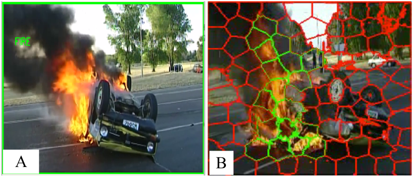
Figure 1: An illustrative example of binary full-frame fire detection (A) and localisation via superpixel segmentation (B) (fire = green, no-fire = red).

Before the advent of deep learning, fire detection work mainly used shallow machine learning approaches using extracted attributes as the input [8, 9, 10]. The work by [8] uses a shallow neural network incorporating a single hidden layer. The model feeds six characteristics of the flame-coloured regions as an input mapping to a hidden layer of seven neurons. A two-class Support Vector Machine (SVM) is used in the work [9] to find a separation between pixels in candidate fire regions to try and remove noise from smoke and differences between frames. Following from this, the work of [10] develops a non-temporal approach that uses a decision tree as the classification architecture, feeding colour-texture feature descriptors as the input, and achieves 80-90% mean true positive detection, 7-8% false positive.

With the advent of deep learning, the focus has shifted from identifying explicit image attributes. A large increase in the classification accuracy has come from creating an end-to-end solution for fire classification [11, 12] and localisation on full-frame/superpixel images (Figure 1), achieved by feeding raw image pixel data as input to a Convolutional Neural Network (CNN) architecture. The work of [11] proposes a custom architecture consisting of convolution, fully connected and pooling layers on a custom dataset using Generative Adversarial Networks (GAN). The work of [12] considers deep CNN architectures such as VGG16 [13] and ResNet50 [14] for the fire detection task. However, these strategies consists of a large number of parameters which lead to slower processing time and may not be suitable for deployment on low-powered embedded devices as commonly found in deployed detection and wide area surveillance systems.

Several CNN architectures [15, 16, 17, 18] are designed to have a low complexity without compromising on the accuracy. The introduction of depth-wise separable convolutions involves splitting up a conventional $H\times W$ filter into a $H\times 1$ depth-wise filter followed by a $1\times W$ point-wise filter, vastly reducing the number of floating-point operations and reducing the overall parameter size in a CNN architecture. Recent advancement in creating compact CNN architectures, which focuses on reducing the overhead costs of computation and parameter storage, involves pruning CNN architectures and compressing the weights of various layers [19, 20] without significantly compromising original accuracy. In the work of [20], a greedy criteria-based pruning of convolutional kernels by backpropagation is proposed. This strategy [20] is computationally efficient and maintains good generalisation in the pruned CNN architecture. An approach by [19] presents acceleration method for CNN architectures, by pruning convolutional filters that are identified as having a small effect on the output accuracy. By removing entire filters in the network with their connecting feature maps, it prevents an increase in sparsity and reduces computational costs. A one-shot pruning and retraining strategy is adopted in this work [19] to save retraining time for pruning filters across multiple layers, which is critical for creating a reduce complexity CNN architecture.

Recent works on non-temporal fire detection [21, 22] outperform the conventional architectures by simplifying a complex high performance, generalised architecture. The FireNet and InceptionV1Onfire are proposed in the work of [21], where the architectures are simplified version of AlexNet [23] and InceptionV1 [24] respectively. Both architectures offer better performance in fire detection over their parent architectures where FireNet [21] achieves $17$ frames per second (fps) with Accuracy of $0.92$ for the binary classification task. Further architectural advancements, InceptionV3 [25] and InceptionV4 [26] architectures are experimentally simplified in the most recent work of [22], which achieves Accuracy of $0.96$ for full-frame and $0.94$ for superpixel classification task. Both architectures achieve high accuracy while maintaining a high computational efficiency and throughput.

In this work, we explicitly consider non-temporal fire detection strategy by proposing significantly reduced complexity CNN architectures compared to prior work of [10, 21, 22]. Our key contributions are the following:

• We propose two simplified compact CNN architectures (NasNet-A-OnFire and ShuffleNetV2-OnFire), which are experimentally defined as architectural subsets of seminal CNN architectures [18, 17] offering maximal performance for the fire detection task.

• We employ the proposed compact CNN architectures for (a) binary fire detection, {fire, no-fire}, in full-frame imagery and (b) in-frame classification and localisation of fire using superpixel segmentation [27].

II Proposed Approach

We consider two CNN architectures, NasNet-A-Mobile [18] and ShuffleNetV2 [17] (Section II-A), which are experimentally optimised using filter pruning [19] for fire detection (Section II-B). Subsequently, we expand this work for in-frame fire localisation via superpixel segmentation (Section II-C).

II-A Reference Architectures

We select NasNet-A-Mobile [18] and ShuffleNetV2 [17] due to their compactness and high performance on ImageNet [28] classification. Both architectures have high level structures, containing normal cell and reduction cell, however with fundamental differences in how these cells are structured at a low level. Due to the modular structures of the architectures, it is easy to remove/modify different cells.

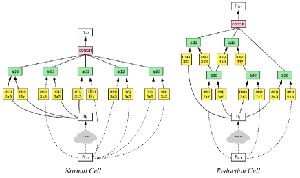
Figure 2: Normal and reduction cells of NasNet-A-Mobile [18].

NasNet-A-Mobile [18] consists of an initial $3\times 3$ convolution layer followed by a sequence repeating three times that consists of a number of reduction cells and four normal cells. The normal and reduction cells (Figure 2), both feed in the input from the previous cell and the cell before, create a residual network. The only convolution layers present in the normal cell are three $3\times 3$ and two $5\times 5$ depth-wise separable convolutions. The reduction cell contains one $3\times 3$, two $5\times 5$, and two $7\times 7$ depth-wise separable convolutions. The rest of the layers are either averaging or max pooling layers.

ShuffleNetV2 [17] consists of an initial $3\times 3$ convolution layer followed by a $3\times 3$ max pooling layer. This is followed by three reduction and normal cells (Figure 3). There is only one reduction cell for each loop and the number of normal cells is $[3,7,3]$. This is followed by a final point-wise convolution and a global pooling layer. The normal cell starts by splitting the number of channels in half, where one half is unchanged and the other half has three convolutions with two point-wise $1\times 1$ convolutions and a $3\times 3$ depth-wise convolution. The output dimension is equal to the input in the normal cell. The channels are concatenated and shuffled in order to mix the channels across the branches. This is applied in both halves of the cells. The reduction cell does not split the channels and both branches receive the whole input. The right branch of the reduction cell is similar to the right branch of the normal cell however the depth-wise convolution has a stride of $2$ to reduce the height and width dimensions by two. The use of point-wise convolutions and depth-wise convolutions allow the network to go very deep without the number of parameters blowing up.

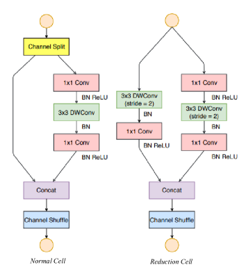
Figure 3: Normal and reduction cell of ShuffleNetV2 [17].

II-B Simplified CNN Architectures

We experimentally investigate variations in architectural configurations of each reference architecture (Section II-A).

In the simplified CNN architectures, we use transfer learning from network models training on ImageNet [28] by removing the final fully connected layer from both architectures [18, 17] and create a new linear layer that mapped to a single value for binary {fire, no-fire} classification. The entire architecture is frozen except the final linear layer for the first half of training. Subsequently, we unfreeze the final convolution layer for ShuffleNetV2 [17], and the final two reductions, normal cell iterations for NasNet-A-Mobile [18]. This prevents the network over-fitting during training and allowing us to train the model longer for better generalisation.

II-B1 Simplified NasNet-A-Mobile

The base model for NasNet-A-Mobile [18] is pre-trained with $1,056$ output channels for ImageNet [28] classification. The main experimentation of this architecture revolves around the number of normal cells in the model.

TABLE I: NasNet-A-Mobile variants with different components.

Architecture	$A_{N}=2$	$A_{N}=4$	$A_{3}=A_{N}$	$A_{3}=0$	Reduced Filter
$NasNet_{v01}$		✓	✓
$NasNet_{v02}$		✓		✓
$\underline{NasNet_{v03}}$	✓		✓
$NasNet_{v04}$	✓			✓
$NasNet_{v05}$		✓	✓		✓
$NasNet_{v06}$		✓		✓	✓
$NasNet_{v07}$	✓		✓		✓
$NasNet_{v08}$	✓			✓	✓

In our simplified NasNet-A-Mobile architectures, we experiment with eight different variants, with four different architectural structure differences with and without reduced filters (Table I). The number of filters is calculated by the number of penultimate filters specified in the architecture. We reduce this number from $1,056$ to $480$ penultimate filters for the reduced filter variants. This creates a reduction of $60\%$ of the filters throughout the whole model. This drastically reduces the number of parameters but achieves a very low accuracy for the each of the reduced filter variants (Figure 4-A). There is a sharp difference in accuracy between the reduced filter variants and full filter variants in the NasNet-A-Mobile architecture [18] (points {a,b,c,d} vs. points {e,f,g,h} in Figure 4-A) with the highest reduce filter variant achieving $0.77$ accuracy compared to $0.95$ for the corresponding full filter variant.

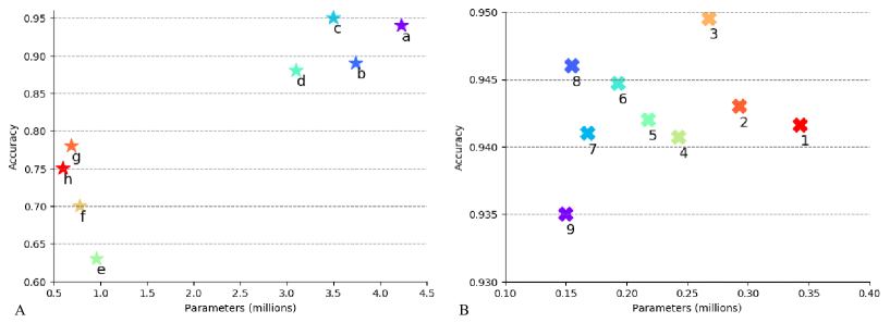
Figure 4: Parameter size and accuracy comparison for the two architecture variants: (A) Nasnet-A-Mobile where a to e represents $NasNet_{v01}$ - $NasNet_{v08}$. (B) ShuffleNetV2 where 1-9 represents $ShuffleNetV2_{v01}$ - $ShuffleNetV2_{v09}$.

II-B2 Simplified ShuffleNetV2

The number parameters in ShuffleNetV2 architecture [17] are $340,000$. Upon examining the distribution of parameters in the architecture, over $200,000$ of the parameters are contained in the final convolutional layer. Therefore we freeze the parameters in the first half of the network and experimentally incorporate the filter pruning strategy to further reduce the complexity of the final convolutional layer, without compromising the accuracy. We adopt a similar approach proposed in the work of [19], which computes the L2-normalisation of the filters, and subsequently we sort and remove the lower valued filters. The intuition behind this strategy is that filters with lower values will be less effective to the final output of the architecture. The model is further retrained with the removed pruned filters.

TABLE II: ShuffleNetV2 [17] pruning variants on the final convolutional filters.

Architecture	Pruned Filters	Final Convolutional Layer Parameters	Total Parameters
$ShuffleNet_{v01}$	128	196,608	342,897
$ShuffleNet_{v02}$	256	147,456	292,897
$ShuffleNet_{v03}$	384	122,800	267,937
$ShuffleNet_{v04}$	512	98,304	242,977
$ShuffleNet_{v05}$	640	73,728	218,017
$ShuffleNet_{v06}$	768	49,152	193,057
$ShuffleNet_{v07}$	896	24,576	168,097
$\underline{ShuffleNet_{v08}}$	960	12,288	155,617
$ShuffleNet_{v09}$	992	6,144	149,377

Table II shows the number of filters pruned in the different variants of the ShuffleNetV2 architecture. We start by pruning $128$ filters that represents $1/8th$ of the number of filters in the final convolutional layer. We remove $128$ filters in each iteration and continued as long as the accuracy does not degrade ($ShuffleNet_{v01}$ to $ShuffleNet_{v07}$). We subsequently prune a further $64$ filters in $ShuffleNet_{v08}$ and $32$ filters in $ShuffleNet_{v09}$ variants however at this stage we stop pruning due to a decrease in accuracy (points 8,9 in Figure 4-B).

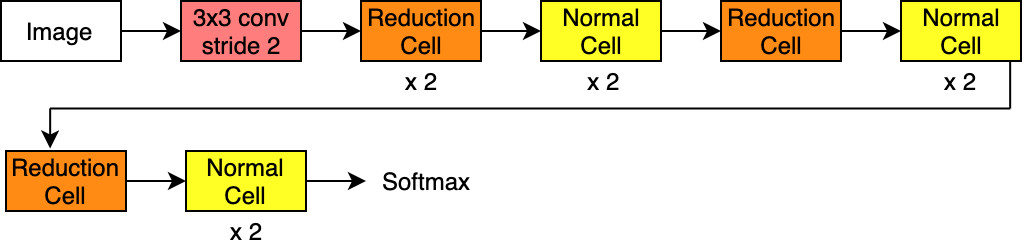
Figure 5: Reduced complexity architecture for NasNet-A-OnFire optimised for fire detection.

With exhaustive experimentation using both architectures, we propose following two reduced complexity architectural variants modified for the binary {fire, no-fire} classification task.

NasNet-A-OnFire is a variant based on $NasNet_{v03}$ such that each group of normal cells in the model only contain two normal cells compared to the previous four (Table I, highlighted in underline). The normal cells and reduction cells in the NasNet-A-OnFire architecture remain the same as shown in Figure 2. The total number of parameter in NasNet-A-OnFire is $3.2$ million.

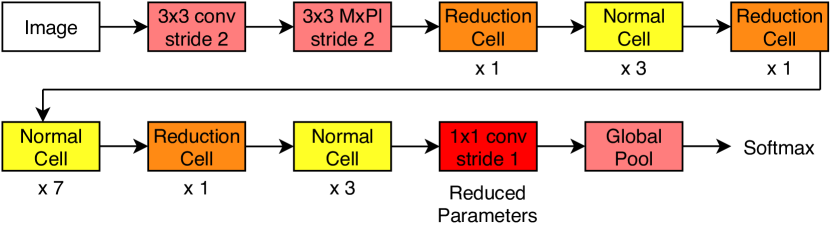
Figure 6: Reduced complexity architecture for ShuffleNetV2-OnFire optimised for fire detection.

ShuffleNetV2-OnFire is a variant of $ShuffleNet_{v08}$ (Table II, highlighted in underline) with the same fundamental architecture design as ShuffleNetV2. In ShuffleNetV2-OnFire (Figure 6), by applying filter pruning strategy, we reduce the number of filters in the final convolutional layer, which leads to a total number of the model parameter of only $155,617$.

We employ these two CNN architectures for {fire, no-fire} classification task applied on full frame binary and superpixel segmentation based fire detection.

II-C Superpixel Localisation

We further expand this work fo in-image fire localisation by using superpixel regions [27], contrary to the earlier work [5, 4] that largely relies on colour based initial locatiosation. Superpixel based techniques over-segment an image into perceptually meaningful regions which are similar in colour and texture. We use Simple Linear Iterative Clustering (SLIC) [27], which performs iterative clustering in a similar manner to k-means to reduced spatial dimensions, where the image is segmented into approximately equally sized superpixels (Figure 1-B). Each superpixel region is classified using proposed NasNet-A-OnFire/ShuffleNetV2-OnFire architecture formulated as a {fire, no-fire}, for fire detection task.

III Evaluation

III-A Experimental Setup

In this section, we present the dataset and implementation details used in our experiments.

III-A1 Dataset

We use the dataset created in the work [21] to train and evaluate the performance of our proposed architectures. The dataset consists of $26,339$ full-frame images (Figure 1-A) of size $224\times 224$, with $14,266$ images of fire, and $12,073$ images of non-fire. Training is performed over a set of $23,408$ images (70 : 20 data split) and testing reported over $2,931$ images. The superpixel (SLIC [27]) training set consists of $54,856$ fire, and $167,400$ non-fire superpixels with a test set of $1178$ fire and $881$ non-fire examples.

III-A2 Implementation Details

The proposed architectures are implemented in PyTorch [29] and trained with the following configuration: backpropagation optimisation performed via Stochastic Gradient Descent (SGD), binary cross entropy loss function, learning rate (lr) of $0.0005$, and $40$ epochs. We measure the performance using the following CPU and GPU configuration: Intel Core i5 with 8GB of RAM CPU, and NVIDIA 2080Ti GPU.

III-B Results

We present the results of the simplified architectures compared to the state-of-the-art for binary classification (Section III-B1) and superpixel localisation task (Section III-B2). For statistically comparing different architectures, we use the metrics of true positive rate (TPR), false positive rate (FPR), F-score (F), Precision (P) and Accuracy (A), Complexity (number of parameters in millions, C), the ratio between accuracy and the number of parameters in the architecture (A:C) and achievable frames per second (fps) throughput.

III-B1 Binary Classification

From the results presented in Table III for full-frame {fire, no-fire} classification task, our proposed architectures achieve comparable performance with prior works [21, 22]. We present only the highest performing variants, NasNet-A-OnFire and ShuffleNetV2-OnFire, in our experimentation (Table III-lower).

TABLE III: The statistical performance for full-frame binary fire detection. Upper: Prior works. Lower: Our approaches.

Architecture	TPR	FPR	F	P	A
FireNet [21]	0.92	0.09	0.93	0.93	0.92
Inception V1-OnFire [21]	0.96	0.10	0.94	0.93	0.93
Inception V3-OnFire [22]	0.95	0.07	0.95	0.95	0.94
Inception V4-OnFire [22]	0.95	0.04	0.96	0.97	0.96
NasNet-A-OnFire	0.92	0.03	0.94	0.96	0.95
ShuffleNetV2-OnFire	0.93	0.05	0.94	0.94	0.95

Both the architectures achieve a FPR less than or equal to the minimum FPR in the current state-of-the-art approaches [21, 22] (Table III-upper) with ShuffleNetV2-OnFire achieving FPR: $0.05$ and NasNet-A-OnFire with FPR: $0.03$ (compared to Inception V4-OnFire [22] with FPR: $0.04$). The overall accuracy remains consistent with both proposed architectures achieving A: $0.95$. Although there is a slight decrease in TPR for both architectures (Table III-lower), still it achieves comparable TPR with prior works considering the compactness and reduced complexity of the architectures as presented in Tables VI and VI. NasNet-A-OnFire offers the best performance in terms of FPR (FPR: 0.03), however ShuffleNetV2-OnFire achieves better TPR with $0.93$. ShuffleNetV2-OnFire outperforms InceptionV3-OnFire [22] at FPR (FPR: 0.05 vs 0.07) and accuracy (A: 0.95 vs 0.94), both being the smallest architectures (Table VI).

III-B2 Superpixel Localisation

For superpixel based fire detection, NasNet-A-OnFire achieves the highest TPR with $0.98$ (Table IV-lower) outperforming the prior work achieving TPR: $0.94$ (InceptionV3-OnFire/InceptionV4-OnFire [22], Table IV-upper). However NasNet-A-OnFire suffers from a high FPR of $0.15$ compared to InceptionV3-OnFire/InceptionV4-OnFire [22] with FPR: 0.07 and FPR: 0.06 respectively. ShuffleNetV2-OnFire achieves a lower FPR (FPR: 0.08, Table IV-lower), which is comparable to prior work [21, 22] and achieves a similar accuracy (A: 0.94). Both of our architectures achieve a higher F-score (F: $0.98$) and Precision (P: $0.99$) outperforming prior work [21, 22].

TABLE IV: Localisation results using within frame superpixel approach. Upper: Prior works. Lower: Our approaches.

Architecture	TPR	FPR	F	P	A
InceptionV1-OnFire [21]	0.92	0.17	0.9	0.88	0.89
InceptionV3-OnFire [22]	0.94	0.07	0.94	0.93	0.94
InceptionV4-OnFire [22]	0.94	0.06	0.94	0.94	0.94
NasNet-A-OnFire	0.98	0.15	0.98	0.99	0.97
ShuffleNetV2-OnFire	0.94	0.08	0.97	0.99	0.94

Qualitative examples of fire localisation, using ShuffleNetV2-OnFire, are illustrated in Figure 7. Each example presents challenging scenarios that could lead to false positive detection. These examples demonstrate the robustness of the proposed architecture for the fire detection task in various challenging scenarios.

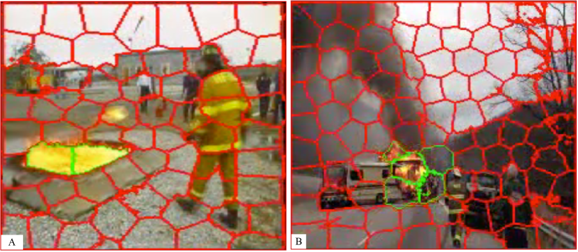
Figure 7: Exemplar superpixel based fire localisation using ShuffleNetV2-OnFire on two challenging scenarios: (A) image containing a fireman wearing an outfit similar colour to the fire and (B) image containing a red colour truck (fire = green, no-fire = red).

III-B3 Architecture Simplification vs Speed

Table VI presents the computational efficiency and speed for full-frame classification using different architectures. ShuffleNetV2-OnFire improves on the computational efficiency by $7.8$ times achieving $608.97$ compared to InceptionV1-OnFire [21] achieving $77.9$ while running on CPU configuration. It also improves on classification speed (fps: $40$) compared to FireNet [21] (fps: $17$), while having $437\times$ fewer number of parameters (C: $0.156$ million), and achieving a higher accuracy (A: $95$%). Whilst computing on a GPU configuration, the inference time increases further for ShuffleNetV2-OnFire achieving $69$ fps, and NasNet-A-OnFire achieves $35$ fps (Table VI-lower). Overall ShuffleNetV2-OnFire is the best performing architecture for full-frame binary classification in terms of accuracy and efficiency (A:C: $608.7$), outperforming prior works [21].

TABLE V: Computational efficiency for full-frame classification.

Architecture	C	A(%)	A:C	fps
FireNet [21]	68.3	91.5	1.3	17
InceptionV1-OnFire [21]	1.2	93.4	77.9	8.4
NasNet-A-OnFire	3.2	95.3	29.78	7
ShuffleNetV2-OnFire	0.156	95	608.97	40
NasNet-A-Mobile (GPU)	3.2	95.3	29.78	35
ShuffleNetV2-OnFire (GPU)	0.156	95	608.97	69

TABLE VI: Computational efficiency for superpixel localisation.

Architecture	C	A(%)	A:C	fps
InceptionV3-OnFire [22]	0.96	94.4	98.09	13.8
InceptionV4-OnFire [22]	7.18	95.6	13.37	12
NasNet-A-OnFire (GPU)	3.2	97.1	30.34	5
ShuffleNetV2-OnFire (GPU)	0.156	94.4	605.13	18

In Table VI, we present the computational efficiency of superpixel localisation (all superpixels are processed for each frame) running on a GPU configuration. Although NasNet-A-OnFire achieves the highest accuracy obtaining A: $97.1$, however it operates at the lowest fps (fps: $5$). ShuffleNetV2-OnFire, consists of only $0.156$ million parameter, provides the maximal throughput of $18$ fps, outperforming InceptionV3-OnFire [22] (fps: $13.8$), as presented in Table VI-lower. We also measure the runtime of our proposed architectures on low-powered embedded device (Nvidia Xavier-NX [30]) as presented in Table VII. The PyTorch implementation operates at a lower speed (fps: 6 & 18) compared to standard CPU/GPU implementation. However, conversion to 16-bit floating point numerical accuracy (via TensorRT, FP16) improves the inference time by $\sim$3-6 times, achieving fps of $35$ (NasNet-A-OnFire) and $49$ (ShuffleNetV2-OnFire), without compromising the performance accuracy.

TABLE VII: Runtime (fps) comparison of {fire, no-fire} classification on different hardware devices.

Architecture	CPU	GPU	Xavier-NX
	PyTorch	PyTorch	PyTorch	TensorRT
NasNet-A-OnFire	7	35	6	35
ShuffleNetV2-OnFire	40	69	18	49

IV Conclusion

We propose a compact and reduced complexity CNN architecture (ShuffleNetV2-OnFire) that is over six times more compact than the prior works [21, 22] for fire detection with a size of $\sim$0.15 million parameters. This significantly outperforms prior works by operating over $\sim$2 times faster. Proposed CNN architectures (NasNet-A-OnFire and ShuffleNetV2-OnFire) are not only compact in size but also achieve similar performance accuracy with $95$% for full-frame and $94.4$% for superpixel based fire detection. Subsequently, implementation on low-powered devices (achieving $49$ fps) makes our architectures suitable for various real-world applications. Overall, we illustrate a strategy for simplifying the CNN architectures through experimental analysis and filter pruning while maintaining the accuracy and increasing the computational efficiency. Future work will focus on additional synthetic image data training via Generative Adversarial Networks.

References

- [1] A. Bardshaw, “The UK security and fire fighting advanced robot project,” in IEE Coll. on Advanced Robotic Initiatives in the UK, London, UK, 1991.
- [2] J. Martinezdedios, L. Merino, F. Caballero, A. Ollero, and D. Viegas, “Experimental results of automatic fire detection and monitoring with UAVs,” Forest Ecology and Management, vol. 234, pp. S232–S232, Nov. 2006.
- [3] G. Healey, D. Slater, T. Lin, B. Drda, and A. Goedeke, “A system for real-time fire detection,” in Proc. Int. Conf. Comp. Vis. and Pat. Rec., 1993, pp. 605–606.
- [4] T. Celik and H. Demirel, “Fire detection in video sequences using a generic color model,” Fire Safety J., vol. 44, no. 2, pp. 147–158, Feb. 2009.
- [5] W. Phillips, M. Shah, and N. da Vitoria Lobo, “Flame recognition in video,” Pat. Rec. Letters, vol. 23, no. 1-3, pp. 319–327, 2002.
- [6] C. Liu and N. Ahuja, “Vision based fire detection,” in Proc. Int. Conf. on Pattern Recognition, 2004, pp. 134–137.
- [7] B. Toreyin, Y. Dedeoglu, and A. Cetin, “Flame detection in video using hidden Markov models,” in Proc. Int. Conf. on Image Proc., 2005, pp. II–1230.
- [8] D. Zhang, S. Han, J. Zhao, Z. Zhang, C. Qu, Y. Ke, and X. Chen, “Image based forest fire detection using dynamic characteristics with artificial neural networks,” in Proc. Int. Joint Conf. on Artificial Intelligence, 2009, pp. 290–293.
- [9] B. Ko, K. Cheong, and J. Nam, “Fire detection based on vision sensor and support vector machines,” Fire Safety J., vol. 44, no. 3, pp. 322–329, Apr. 2009.
- [10] A. Chenebert, T. P. Breckon, and A. Gaszczak, “A non-temporal texture driven approach to real-time fire detection,” in Proc. Int. Conf. on Image Proc., Sep. 2011, pp. 1741–1744.
- [11] A. Namozov and Y. Im Cho, “An efficient deep learning algorithm for fire and smoke detection with limited data,” Advances in Electrical and Computer Engineering, vol. 18, no. 4, pp. 121–129, 2018.
- [12] J. Sharma, O.-C. Granmo, M. Goodwin, and J. T. Fidje, “Deep convolutional neural networks for fire detection in images,” in International Conference on Engineering Applications of Neural Networks. Springer, 2017, pp. 183–193.
- [13] K. Simonyan and A. Zisserman, “Very deep convolutional networks for large-scale image recognition,” in In Proc. Int. Conf. on Learning Representations, 2015.
- [14] K. He, X. Zhang, S. Ren, and J. Sun, “Deep residual learning for image recognition,” in Proc. Computer Vision and Pattern Recognition, 2016, pp. 770–778.
- [15] F. N. Iandola, M. W. Moskewicz, K. Ashraf, S. Han, W. J. Dally, and K. Keutzer, “Squeezenet: Alexnet-level accuracy with 50x fewer parameters and <1mb model size,” CoRR, vol. abs/1602.07360, 2016.
- [16] A. G. Howard, M. Zhu, B. Chen, D. Kalenichenko, W. Wang, T. Weyand, M. Andreetto, and H. Adam, “Mobilenets: Efficient convolutional neural networks for mobile vision applications,” CoRR, vol. abs/1704.04861, 2017.
- [17] N. Ma, X. Zhang, H.-T. Zheng, and J. Sun, “Shufflenet v2: Practical guidelines for efficient CNN architecture design,” in Proc. of the European Conference on Computer Vision, 2018, pp. 122–138.
- [18] B. Zoph, V. Vasudevan, J. Shlens, and Q. V. Le, “Learning transferable architectures for scalable image recognition,” in In Proc. of Computer vision and pattern recognition, 2018, pp. 8697–8710.
- [19] H. Li, A. Kadav, I. Durdanovic, H. Samet, and H. P. Graf, “Pruning filters for efficient convnets,” in In Proc. Int. Conf. on Learning Representations, 2017.
- [20] P. Molchanov, S. Tyree, T. Karras, T. Aila, and J. Kautz, “Pruning convolutional neural networks for resource efficient transfer learning,” in In Proc. Int. Conf. on Learning Representations, 2017.
- [21] A. Dunnings and T. Breckon, “Experimentally defined convolutional neural network architecture variants for non-temporal real-time fire detection,” in Proc. Int. Conf. on Image Processing. IEEE, September 2018, pp. 1558–1562.
- [22] G. S. C.A., N. Bhowmik, and T. P. Breckon, “Experimental exploration of compact convolutional neural network architectures for non-temporal real-time fire detection,” in Proc. Int. Conf. On Machine Learning And Applications, 2019, pp. 653–658.
- [23] A. Krizhevsky, I. Sutskever, and G. E. Hinton, “Imagenet classification with deep convolutional neural networks,” in Advances in Neural Information Processing Systems 25. Curran Associates, Inc., 2012, pp. 1097–1105.
- [24] C. Szegedy, Wei Liu, Yangqing Jia, P. Sermanet, S. Reed, D. Anguelov, D. Erhan, V. Vanhoucke, and A. Rabinovich, “Going deeper with convolutions,” in Proc. Conf. on Computer Vision and Pattern Recognition, 2015, pp. 1–9.
- [25] C. Szegedy, V. Vanhoucke, S. Ioffe, J. Shlens, and Z. Wojna, “Rethinking the inception architecture for computer vision,” in Proc. Computer Vision and Pattern Recognition, 2016, pp. 2818–2826.
- [26] C. Szegedy, S. Ioffe, V. Vanhoucke, and A. A. Alemi, “Inception-v4, inception-resnet and the impact of residual connections on learning,” 2017, p. 4278–4284.
- [27] R. Achanta, A. Shaji, K. Smith, A. Lucchi, P. Fua, and S. Süsstrunk, “Slic superpixels compared to state-of-the-art superpixel methods,” IEEE Trans Pattern Analysis and Machine Intelligence, vol. 34, no. 11, pp. 2274–2282, 2012.
- [28] J. Deng, W. Dong, R. Socher, L. Li, K. Li, and L. Fei-Fei, “Imagenet: A large-scale hierarchical image database,” in Proc. Computer Vision and Pattern Recognition, 2009, pp. 248–255.
- [29] A. Paszke, S. Gross, F. Massa, A. Lerer, J. Bradbury, G. Chanan, T. Killeen, Z. Lin, N. Gimelshein, L. Antiga et al., “Pytorch: An imperative style, high-performance deep learning library,” in Advances in Neural Information Processing Systems, 2019, pp. 8024–8035.
- [30] “Nvidia Jetson Xavier NX,” https://developer.nvidia.com/embedded/jetson-xavier-nx, accessed: 2020-09-29.