Microscopical justification of Solid-State
Wetting and Dewetting

Abstract.

The continuum model related to the Winterbottom problem, i.e., the problem of determining the equilibrium shape of crystalline drops resting on a substrate, is derived in dimension two by means of a rigorous discrete-to-continuum passage by $\Gamma$-convergence of atomistic models taking into consideration the atomic interactions of the drop particles both among themselves and with the fixed substrate atoms. As a byproduct of the analysis effective expressions for the drop surface anisotropy and the drop/substrate adhesion parameter appearing in the continuum model are characterized in terms of the atomistic potentials, which are chosen of Heitmann-Radin sticky-disc type. Furthermore, a threshold condition only depending on such potentials is determined distinguishing the wetting regime, where discrete minimizers are explicitly characterized as configurations contained in a layer with a one-atom thickness, i.e., the wetting layer, on the substrate, from the dewetting regime. In the latter regime, also in view of a proven conservation of mass in the limit as the number of atoms tends to infinity, proper scalings of the minimizers of the atomistic models converge (up to extracting a subsequence and performing translations on the substrate surface) to a bounded minimizer of the Winterbottom continuum model satisfying the volume constraint.

1. Introduction

The problem of determining the equilibrium shape formed by crystalline drops resting upon a rigid substrate possibly of a different material is long-standing in materials science and applied mathematics. The first phenomenological prediction of such shape for flat substrates is due to W. L. Winterbottom, who in [36] designed what is now referred to as the Winterbottom construction (see Figure 1) to minimize the drop surface energy in which both the drop anisotropy at the free surface and the drop wettability at the contact region with the substrate were taken into account (see (1) below). The interplay between the drop material properties of anisotropy and wettability can induce different morphologies ranging from the spreading of the drops in a infinitely thick wetting layer covering the substrate, which is exploited, e.g., in the design of film coatings, to the nucleation of dewetted islands, that are solid-state clusters of atoms leaving the substrate exposed among them, which find other applications, such as for sensor devices and as catalysts for the growth of carbon and semiconductor nanowires [19, 20].

In this work we introduce a discrete setting dependent on the atomistic interactions of drop particles both among themselves and with the substrate particles, and we characterize in terms of the parameters of the potentials governing such atomistic interactions the regime associated with the wetting layer, referred in the following as the wetting regime. For the complementary parameter range, i.e., the dewetting regime, we microscopically justify the formation of solid-state dewetted islands by performing a rigorous discrete-to-continuum passage by means of showing the $\Gamma$-convergence of the atomistic energies to the energy considered in [19, 20] and by W. L. Winterbottom in [36].

In the continuum setting, the Winterbottom problem in [36] essentially consists in an optimization problem based on an a priori knowledge of the surface anisotropy $\Gamma$ of the resting crystalline drop with the surrounding vapor, and of the adhesivity $\sigma$ related to the contact interface between the drop and the substrate. In the modern mathematical formulation in $\mathbb{R}^{d}$ for $d>1$ the energy associated to an admissible region $D\subset\mathbb{R}^{d}\setminus S$ occupied by the drop material, which is assumed to be a set of finite perimeter outside a fixed smooth substrate region $S\subset\mathbb{R}^{d}$, is given by

$$\mathcal{E}(D):=\int_{\partial^{*}D\setminus\partial S}\Gamma(\nu(\xi))\,\mathrm{d}\mathcal{H}^{d-1}(\xi)+\sigma\mathcal{H}^{1}(\partial^{*}D\cap\partial S),$$ (1)

where $\partial^{*}D$ is the reduced boundary of $D$, $\nu$ is the exterior normal vector of $D$, and $\mathcal{H}^{d-1}$ the $(d-1)$-dimensional measure. The Winterbottom shape $W_{\Gamma,\sigma}$ introduced in [36] is defined as depicted in Figure 1 by

$$W_{\Gamma,\sigma}:=W_{\Gamma}\cap\{x\in\mathbb{R}^{d}\,:\,x_{d}\geq-\sigma\}$$

where $W_{\Gamma}$ is the Wulff shape, i.e.,

$$W_{\Gamma}:=\{x\in\mathbb{R}^{d}\,:\,x\cdot\nu\leq\Gamma(\nu)\text{ for every }\nu\in S^{d-1}\}.$$

The Wulff shape $W_{\Gamma}$ is named after G. Wulff, who provided in [37] its first phenomenological construction as the equilibrium shape for a free-standing crystal with anisotropy $\Gamma$ in the space (in the absence of a substrate or any other crystalline materials), and was afterwards in [13, 15] rigorously proved to be the unique minimum of (1) when $S=\emptyset$ in the presence of a volume constraint and after a proper scaling to adjust its volume (see also [34, 35]).

The emergence of the Wulff and Winterbottom shapes have been already justified starting from discrete models in the context of statistical mechanics and the Ising model. We refer to the review [11] (see also [18, 22]) for the 2-dimensional derivation of the Wulff shape in the scaling limit at low-temperature and to [5, 29, 30] for the setting related to the Winterbottom shape. More recently, the microscopical justification of the Wulff shape in the context of atomistic models depending on Heitmann-Radin sticky-disc type potentials [17] has been addressed for $d=2$ and the triangular lattice in [3] by performing a rigorous discrete-to-continuum analysis by means of $\Gamma$-convergence. Subsequetly, the deviation of discrete ground states in the triangular lattice from the asymptotic Wulff shape has been sharply quantified in [31] by introducing the $n^{3/4}$ law (see also [10]), which has been then extended to the square lattice in [26, 27], to the hexagonal lattice for graphene nanoflakes in [9], and to higher dimensions in [25, 28].

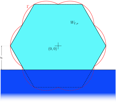
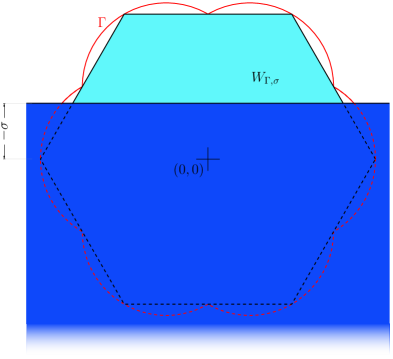
Figure 1. Winterbottom construction for the minimizer of $\mathcal{E}$, on the left for $\sigma>0$ and on the right for $\sigma<0$ (see [36]).

We intend here to generalize the analysis of [3] for $d=2$ to the situation of $S\neq\emptyset$ by taking into account at the discrete level also the atomic interactions of the particles of the crystalline drops with the particles of the substrate, which we allow to possibly belong to a different species of particles, and we suppose occupying all sites of a fixed reference lattice $\mathcal{L}_{S}\subset S$. Film atoms are instead let free to move in a lattice $\mathcal{L}_{F}$ chosen to be triangular and contained in $\mathbb{R}^{2}\setminus\overline{S}$, so that admissible configurations of crystalline drops with $n\in\mathbb{N}$ film atoms are $D_{n}:=\{x_{1},\ldots,x_{n}\}\subset\mathcal{L}_{F}$ (see Figure 2). By adding the contribution $E_{S}:(\mathbb{R}^{2}\setminus\overline{S})^{n}\to\mathbb{R}\cup\{\infty\}$ to the energy of [3] to include atomic interactions of film atoms with substrate atoms, the overall energy $V_{n}$ of an admissible configuration $D_{n}:=\{x_{1},\ldots,x_{n}\}$ is given by

$$V_{n}(D_{n})=V_{n}(x_{1},\ldots,x_{n}):=E_{F}(D_{n})+E_{S}(D_{n}),$$

where $E_{F}:(\mathbb{R}^{2}\setminus\overline{S})^{n}\to\mathbb{R}\cup\{\infty\}$ represents the contribution of the atomic interactions among film atoms. More precisely, $E_{F}$ and $E_{S}$ are defined by

$$E_{F}(D_{n})=E_{F}(x_{1},\ldots,x_{n}):=\color[rgb]{0,0,0}\sum_{i\neq j}v_{FF}(|x_{i}-x_{j}|)$$

and

$$E_{S}(D_{n})=E_{S}(x_{1},\dots,x_{n}):=\sum_{i=1}^{n}\sum_{s\in\mathcal{L}_{S}}v_{\textrm{FS}}(|x_{i}-s|),$$

respectively, where $v_{F\alpha}$ for $\alpha=F,S$ are Heitmann-Radin sticky-disc two-body potentials attaining their minimum values $-c_{\alpha}$ at $e_{\alpha}>0$, where $e_{\alpha}$ is the distance between nearest neighbors in $\mathcal{L}_{\alpha}$ (see Figure 2).

We recall that even with Heitmann-Radin potentials the crystallization of the minimizers of $V_{n}$ has been shown so far only in the case with $S=\emptyset$ in [17] by showing that the minimizers of $E_{F}$ are subset of a triangular lattice. The rigidity assumption of prescribing reference lattices $\mathcal{L}_{F}$ and $\mathcal{L}_{S}$, besides imposing the non-interpenetration for the film and substrate species of atoms, which remain separated by $\partial S$, also entails that the elastic energy associated to the mismatch between the optimal crystalline lattices of the two materials of the drop and the substrate at equilibrium is supposed to be all released by means of the periodic dislocations of the global reference lattice $\mathcal{L}:=\mathcal{L}_{F}\cup\mathcal{L}_{S}$ prescribed at the film-substrate interface $\partial S$. A study in which the complementary situation where elastic deformations of a homogeneous reference lattice $\mathcal{L}$ without dislocations between the film and the substrate are considered, is available in [23], where the linear-elastic models for epitaxially-strained thin films introduced in [7, 8, 14, 32, 33] are derived from nonlinear elastic atomistic energies.

In our setting due to the periodic dislocations created at the interface between $\mathcal{L}_{F}$ and $\mathcal{L}_{S}$ the substrate interactions included in $E_{S}$ are in general non-constant (if not when $e_{F}$ is a multiple of $e_{S}$) and may result in periodic oscillations between null and negative contributions to the overall energy, referred to in the following as periodic adhesion deficit. The presence of such oscillations substantiate the employment of homogenization techniques for periodic structures (see [2] for the continuum setting), which represents one of the difference with the analysis carried out in [3]. It then turns out though that the homogenized limit actually coincide with the average in our setting (and in [6] in the continuum setting).

Moreover, the periodic adhesion deficit at the drop/substrate region induces a lack of compactness for (the properly scaled) energy-equi-bounded sequences (even up to uniform translations), which is not treatable with only adopting local arguments at the substrate surface similar to the one employed in [3]. In order to balance up the deficit we subdivide drop configurations in strips vertical to the substrate so that enough boundary particles not adhering with the substrate (and so without deficit) are counted. Then, summing out all the strips allows to determine a global lower bound to the overall surface contribution and to recover compactness in a proper subclass of admissible configurations, i.e., almost-connected configurations (see Section 2.4), that are configurations union of connected components positioned at “substrate-bond” distance. Such limitation is then overcome by means of ensuring that mass does not escape on the infinite substrate surface.

Another reason for the lack of compactness with substrate interactions is the possibility for minimizing drop configurations to spread out on the infinite substrate surface forming an infinitesimal wetting layer, which for $E_{S}\not\equiv 0$ can be actually favored. Therefore, a peculiar aspect of our analysis resides in distinguishing such wetting regime from the dewetting regime. More precisely, we characterize a dewetting threshold in terms of the interatomic potentials $v_{FF}$ and $v_{FS}$, namely

$$\begin{cases}c_{S}<4c_{F}&\text{if $e_{F}$ is a multiple of $e_{S}$,}\\ c_{S}<6c_{F}&\text{otherwise,}\end{cases}$$ (2)

under which the emergence of the minimizers of (1) with full $\mathbb{R}^{2}$-Lebesgue measure is shown.

The results of the paper are threefold (see Section 2.6): The first result, Theorem 2.2, is a crystallization result for wetting configurations achieved by induction arguments in which the dewetting-threshold condition (2) is singled out by treating separately the situation of constant and non-constant substrate contributions. In this regard notice that the characterization of the dewetting regime coming from continuum theories (see, e.g., [4]) does not represent in general a good prediction for the discrete setting due to the deficit averaging effects taking place in the passage from discrete to continuum. More precisely, as described in [4] (with the extra presence of a gravity-term perturbation of $\mathcal{E}$) the condition

$$\sigma>-\Gamma(\nu_{S})$$ (3)

is the natural requirement in the continuum “ensuring that it is not energetically preferred for minimizers to spread out into an infinitesimally thin sheet”. However, condition (3) coincides with the dewetting-threshold condition of the discrete setting only when $e_{F}$ is a multiple of $e_{S}$ (see (5) and (6) below), being otherwise the latter condition more restrictive.

The second result, Theorem 2.3, provides a conservation of mass for the solutions of the discrete minimum problems

$$\min_{D_{n}\subset\mathcal{L}_{F}}{V_{n}(D_{n})}\$$ (4)

as the number $n$ of atoms tends to infinity, which is crucial to overcome the lack of compactness outside the class of almost-connected sequences of energy-equibounded minimizers. In particular, it consists in proving that it is enough to select a connected component among those with largest cardinality for each solution of (4). This is achieved by proving compactness for almost-connected energy minimizers and then by defining a proper transformation $\mathcal{T}$ of configurations (based on iterated translations of connected components as detailed in Definition 2.1), which always allows to pass to an almost-connected sequence of minimizers.

The last result, Theorem 2.4, relates to the convergence of the minimizers of (4) as $n\to\infty$ to a minimizer of (1) in the family of crystalline-drop regions

$$\mathcal{D}_{\rho}:=\{D\subset\mathbb{R}^{2}\setminus S\,:\,\text{set of finite perimeter, bounded and such that $|D|=1/\rho$}\},$$

whose existence follows also from the proof, where $\rho$ is the atom density in $\mathcal{L}_{F}$ per unit area. Such convergence is obtained (up to extracting a subsequence and performing horizontal translations on the substrate $S$) as a direct consequence of the conservation of mass provided by Theorem 2.3 and of a $\Gamma$-convergence result for properly defined versions of $V_{n}$ and $\mathcal{E}$ in the space $\mathcal{M}(\mathbb{R}^{2})$ of Radon measures on $\mathbb{R}^{2}$ with respect to the weak* convergence of measures as the number $n$ of film atoms tends to infinity.

More precisely, we consider the one-to-one correspondence between drop configurations $D_{n}\subset\mathcal{L}_{F}$ and their associated empirical measures $\mu_{D_{n}}\in\mathcal{M}(\mathbb{R}^{2})$ (see definition at (12)), introduce an energy $I_{n}$ defined in $\mathcal{M}(\mathbb{R}^{2})$ such that

$$I_{n}(\mu_{D_{n}})=V_{n}(D_{n}),$$

and prove that the $\Gamma$-convergence of proper scalings $E_{n}$ of $I_{n}$, namely

$$E_{n}:=n^{-1/2}(I_{n}+6c_{F}n),$$

with respect to the weak* convergence of measures, to a functional $I_{\infty}$ defined in such a way that

$$I_{\infty}\left(\rho\chi_{D}\right)=\mathcal{E}(D),$$

for every sets of finite perimeter $D\subset\mathbb{R}^{2}\setminus S$ with $|D|=1/\rho$ and for specific effective expressions of the surface tension $\Gamma$ and of the adhesivity $\sigma$ appearing in the definition (1) of $\mathcal{E}$ in terms of the interatomic potentials $v_{FF}$ and $v_{FS}$. In particular, we obtain that

$$\sigma:=2c_{F}-\frac{c_{S}}{q},$$ (5)

where $q$ relates to the proportion between $e_{F}$ and $e_{S}$ (see (11)), and $\Gamma(\nu(\cdot))$ is found to be the $\pi/3$-periodic function such that

$$\Gamma(\nu(\varphi)):=2c_{F}\left(\nu_{2}(\varphi)-\frac{\nu_{1}(\varphi)}{\sqrt{3}}\right)$$ (6)

for every

$$\nu(\varphi)=\left(\begin{array}[]{c}-\sin\varphi\\ \cos\varphi\end{array}\right)$$

with $\varphi\in[0,\pi/3]$.

A crucial difference with respect to [3] in the proof of the lower and upper bound of such $\Gamma$-convergence result is that the adhesion term in (1) can be negative and originates in view of the averaging of the periodic adhesion deficit related to the dislocations at the film-substrate interface. In particular, it is the limit of the adhesion portion of the boundary of auxiliary sets $H_{n}^{\prime}$ associated to the configurations $D_{n}$ (see definition (53) based on lattice Voronoi cells) in the oscillatory sets $O_{n}$ (see Figure 2). We notice that for such averaging arguments extra care is needed, as the results available from the continuum theories cannot directly be applied to the auxiliary sets $H_{n}^{\prime}$ when $e_{F}$ is not a multiple of $e_{S}$, e.g., with respect to [4] (see also [6]) because of the non-constant deficit, and with respect to [2] when $4c_{F}\leq c_{S}<6c_{F}$ because of the discrepancy between the continuum and the discrete dewetting conditions.

Finally, we observe that as a consequence of the $\Gamma$-convergence result contained in Theorem 2.4, not only the convergence of global minimizers of (4) to a minimizer of (1), but also the convergence of isolated local (with respect to a proper topology) minimizers of $E_{n}$ to an isolated local minimizer of (1) as $n\to\infty$ is entailed (see, e.g., [21]). In this regard, we refer to [19, 20] for the importance of detecting the local equilibrium shapes related to energies of type (1), especially in relation to the various kinetic phenomena affecting the dewetting dynamics, such as Rayleigh-like instabilities, corner-induced instabilities, and periodic mass-shedding.

1.1. Paper organization

In Section 2 we introduce the mathematical setting with the discrete models (expressed both with respect to lattice configurations and to Radon measures) and the continuum model, and the three main theorems of the paper. In Section 3 we treat the wetting regime and prove Theorem 2.2. In Section 4 we establish the compactness result for energy-$E_{n}$-equibounded almost-connected sequences. In Section 5 we prove the lower bound of the $\Gamma$-convergence result. In Section 6 we prove the upper bound of the $\Gamma$-convergence result. In Section 7 we study the convergence of almost-connected transformations of minimizers and present the proofs of both Theorems 2.3 and 2.4. Finally, an Appendix with specific auxiliary results particularly important in the various proofs is added for the Reader’s convenience.

2. Mathematical setting and main results

In this section we rigorously introduce the discrete and continuous models, the notation and definitions used throughout the paper, and the main results.

2.1. Setting with lattice configurations

We begin by introducing a reference lattice $\mathcal{L}\subset\mathbb{R}^{2}$ for the atoms of the substrate and of the film, which we assume to remain separate. We define $\mathcal{L}:=\mathcal{L}_{S}\cup\mathcal{L}_{F}$, where $\mathcal{L}_{S}\subset\overline{S}$ denotes the reference lattice for the substrate atoms, $S:=\mathbb{R}\times\{r\in\mathbb{R}\,:\,r<0\}$ is referred to as the substrate region, and $\mathcal{L}_{F}\subset\mathbb{R}^{2}\setminus\overline{S}$ is the reference lattice for the film atoms.

More precisely, we consider the substrate lattice as a fixed lattice, i.e., every lattice site in $\mathcal{L}_{S}$ is occupied by a substrate atom, such that

$$\partial\mathcal{L}_{S}:=\mathcal{L}_{S}\cap\{(r,0):\,r\in\mathbb{R}\,\}=\{s_{k}:=(ke_{S},0)\,:\,k\in\mathbb{Z}\}$$

for a positive lattice constant $e_{S}$, and we refer to $\partial\mathcal{L}_{S}$ as to the substrate surface (or wall). For the film lattice $\mathcal{L}_{F}$ we choose a triangular lattice with parameter $e_{F}$ normalized to 1, namely

$$\mathcal{L}_{F}:=\{x_{F}+k_{1}\bm{t}_{1}+k_{2}\bm{t}_{2}\,:\,\color[rgb]{0,0,0}\textrm{$k_{1}\in\mathbb{Z}$ and $k_{2}\in\mathbb{N}\cup\{0\}$}\color[rgb]{0,0,0}\}$$

where $x_{F}:=(0,e_{S})$,

$$\bm{t}_{1}:={1\choose 0},\quad\textrm{and}\quad\bm{t}_{2}:=\color[rgb]{0,0,0}\frac{1}{2}{1\choose\sqrt{3}}.$$

We denote by $\partial\mathcal{L}_{F}$ the lower boundary of the film lattice, i.e.,

$$\partial\mathcal{L}_{F}:=\{x_{F}+k_{1}\bm{t}_{1}:\,\color[rgb]{0,0,0}\textrm{$k_{1}\in\mathbb{Z}$}\color[rgb]{0,0,0}\}$$

and by $\partial\mathcal{L}_{FS}$ the collection of sites in the lower boundary of the film lattice at a distance of $e_{S}$ from an atom in $\partial\mathcal{L}_{S}$, i.e.,

$$\partial\mathcal{L}_{FS}:=\partial\mathcal{L}_{F}\cap\left(\partial\mathcal{L}_{S}+e_{S}\bm{t}_{3}\right)$$

where

$$\bm{t}_{3}:={0\choose 1}$$

(see Figure 2).

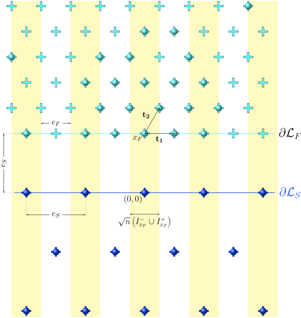
Figure 2. A portion of the lattices $\mathcal{L}_{F}$ and $\mathcal{L}_{S}$ is depicted with the respective lattice sites in light and dark blue crosses, respectively. The lattice $\mathcal{L}_{S}$ is fully occupied by substrate atoms represented by dark blue balls, while only some sites of $\mathcal{L}_{F}$ are occupied by film atoms represented by light blue balls. The “interface” $\partial\mathcal{L}_{F}$ consists of all the lattice sites on the light-blue line, while the “interface” $\partial\mathcal{L}_{S}$ consists of all the lattice sites on the dark-blue line. In yellow we can see the oscillatory set related to the lattice sites in $\partial\mathcal{L}_{FS}$, which is introduced in Section 5.

The sites of the film lattice are not assumed to be completely filled and we refer to a set of $n\in\mathbb{N}$ sites $x_{1},\dots,x_{n}\in\mathcal{L}_{F}$ occupied by film atoms as a crystalline configuration denoted by $D_{n}:=\{x_{1},\dots,x_{n}\}\subset\mathcal{L}_{F}$. Notice that the labels for the elements of a configuration $D_{n}$ are uniquely determined by increasingly assigning them with respect to a chosen fixed order on the lattice sites of $\mathcal{L}_{F}$. With a slight abuse of notation we refer to $x\in D_{n}$ as an atom in $D_{n}$ (or in $\mathcal{L}_{F}$). We denote the family of crystalline configurations with $n$ atoms by $\mathcal{C}_{n}$. Furthermore, given a set $A\subset\mathbb{R}^{2}$, its cardinality is indicated by $\#A$, so that

$$\mathcal{C}_{n}:=\{A\subset\mathcal{L}_{F}\,:\,\#A=n\}.$$

For every atom $x\in\mathcal{L}_{F}$ we take into account both its atomistic interactions with other film atoms and with the substrate atoms, by considering the two-body atomistic potentials $v_{FF}$ and $v_{FS}$, respectively. We restrict to first-neighbor interactions and we define $v_{F\alpha}$ for $\alpha:=F,S$ as

$$v_{F\alpha}(r):=v_{\alpha}(r)$$

where $v_{\alpha}$ are the Heitmann-Radin potentials defined for $\alpha:=F,S$ by

$$v_{\alpha}(r):=\begin{cases}+\infty&\mbox{if }r<e_{\alpha},\\ -c_{\alpha}&\mbox{if }r=e_{\alpha},\\ 0&\mbox{if }r>e_{\alpha}.\end{cases}$$ (7)

with $c_{\alpha}$ and $e_{\alpha}$ positive constants.

In the following, we refer to film and substrate neighbors of an atom $x$ in a configuration $D_{n}$ as to those atoms in $D_{n}$ at distance 1 from $x$, and to those atoms in $\mathcal{L}_{S}$ at distance $e_{S}$ from $x$, respectively. Analogously, we refer to film and substrate bonds of an atom $x$ in a configuration $D_{n}$ as to those segments connecting $x$ to its film and substrate neighbors, respectively. We also refer to the union of the closures of all film bonds of atoms in a configuration $D_{n}$ as the bonding graph of $D_{n}$, and we say that a crystalline configuration $D_{n}$ is connected if every $x$ and $y$ in $D_{n}$ are connected through a path in the bonding graph of $D_{n}$, i.e., there exist $\ell\leq n$ and $x_{k}\in D_{n}$ for $k:=1,\dots,\ell$ such that $|x_{k}-x_{k-1}|=1$, $x_{1}=x$, and $x_{\ell}=y$. Moreover, we define the boundary of a configuration $D_{n}\in\mathcal{C}_{n}$ as the set $\partial D_{n}$ of atoms of $D_{n}$ with less than 6 film neighbors. We notice here that with a slight abuse of notation, given a set $A\subset\mathbb{R}^{2}$ the notation $\partial A$ will also denote the topological boundary of a set $A\subset\mathbb{R}^{2}$ (which we intend to be always the way to interpret the notation when applied not to configurations in $\mathcal{C}_{n}$, or to lattices, such as for $\partial\mathcal{L}_{S}$, $\partial\mathcal{L}_{F}$, and $\partial\mathcal{L}_{FS}$).

The energy $V_{n}$ of a configuration $D_{n}:=\{x_{1},\ldots,x_{n}\}\subset\mathcal{L}_{F}$ of $n$ particles is defined by

$$\color[rgb]{0,0,0}V_{n}(D_{n})=\color[rgb]{0,0,0}V_{n}(x_{1},\ldots,x_{n})\color[rgb]{0,0,0}:=\color[rgb]{0,0,0}\sum_{i\neq j}v_{FF}(|x_{i}-x_{j}|)\,+\,E_{S}(x_{1},\ldots,x_{n})\color[rgb]{0,0,0}$$ (8)

where $E_{S}:(\mathbb{R}^{2}\setminus\overline{S})^{n}\color[rgb]{0,0,0}\to\mathbb{R}\cup\{\infty\}$ represents the overall contribution of the substrate interactions defined as

$$E_{S}(D_{n})=E_{S}(x_{1},\dots,x_{n}):=\sum_{i=1}^{n}v^{1}(x_{i}),$$ (9)

where the one-body potential $v^{1}$ is defined by

$$v^{1}(x):=\sum_{s\in\mathcal{L}_{S}}v_{\textrm{FS}}(|x-s|)$$ (10)

for any $x\in\mathbb{R}\times\{r\in\mathbb{R}\,:\,r>0\}$. Notice that from the definition of $v_{FS}$ and $x_{F}$ for any $x\in\mathcal{L}_{F}$ the sum in (10) is finite and

$$v^{1}(x)\in\{0,-c_{S}\}.$$

In the following we will always focus on the case

$$e_{S}:=\frac{q}{p}$$ (11)

for some $p,q\in\mathbb{N}$ without common factors, since the case of $e_{S}=re_{F}$ for some $r\in\mathbb{R}\setminus\mathbb{Q}$ is simpler, as the contribution of $E_{S}$ is negligible. More precisely, for $e_{S}=re_{F}$ with $r\in\mathbb{R}\setminus\mathbb{Q}$ the same analysis (or the one in [3]) applies, and, up to rigid transformations, minimizers converge to a Wulff shape in $\mathbb{R}^{2}\setminus S$ with the Wulff-shape boundary intersecting $\partial S$ at least in a point.

We also notice that the setting in which $\mathcal{L}_{F}$ is replaced by

$$\mathcal{L}^{\prime}_{F}:=\mathcal{L}_{F}+\left(\frac{e_{S}}{2},\frac{\sqrt{3}e_{S}}{2}-e_{S}\right)$$

where each atom in $\partial\mathcal{L}_{FS}$ may present up to two (instead of one) bonds with $\mathcal{L}_{S}$ (which are obliques instead of in $\bm{t}_{3}$ direction) is analogous and the same arguments of the paper lead to the corresponding $\Gamma$-convergence result.

2.2. Setting with Radon measures

The $\Gamma$-convergence result is established for a version of the previously described discrete model expressed in terms of empirical measures since it is obtained with respect to the weak* topology of Radon measures [1]. We denote the space of Radon measures on $\mathbb{R}^{2}$ by $\mathcal{M}(\mathbb{R}^{2})$ and we write $\mu_{n}\stackrel{{\scriptstyle*}}{{\rightharpoonup}}\mu$ to denote the convergence of a sequence $\{\mu_{n}\}\subset\mathcal{M}(\mathbb{R}^{2})$ to a measure $\mu\in\mathcal{M}(\mathbb{R}^{2})$ with respect to the weak* convergence of measures. The empirical measure $\mu_{D_{n}}$ associated to a configuration $D_{n}:=\{x_{1},\dots,x_{n}\}\in\mathcal{C}_{n}$ is defined by

$$\mu_{D_{n}}:=\frac{1}{n}\sum_{i=1}^{n}\delta_{\frac{x_{i}}{\sqrt{n}}},$$ (12)

where $\delta_{z}$ represents the Dirac measure concentrated at a point $z\in\mathbb{R}^{2}$, and the family of empirical measures related to configurations in $\mathcal{C}_{n}$ is denoted by $\mathcal{M}_{n}$, i.e.,

$$\mathcal{M}_{n}:=\{\mu\in\mathcal{M}(\mathbb{R}^{2})\ :\ \text{there exists $D_{n}\in\mathcal{C}_{n}$ such that $\mu=\mu_{D_{n}}$}\}.$$ (13)

The functional $I_{n}$ associated to the configurational energy $V_{n}$ and expressed in terms of Radon measures is given by

$$I_{n}(\color[rgb]{0,0,0}\mu\color[rgb]{0,0,0})\color[rgb]{0,0,0}:=\color[rgb]{0,0,0}\left\{\begin{array}[]{lll}\int_{(\color[rgb]{0,0,0}\mathbf{R}^{2}\setminus\overline{S}\color[rgb]{0,0,0})^{2}\backslash\textrm{diag}}n^{2}v_{FF}(n^{1/2}|x-y|)d\mu\color[rgb]{0,0,0}(x)\color[rgb]{0,0,0}\otimes d\mu\color[rgb]{0,0,0}(y)&&\quad\textrm{\color[rgb]{0,0,0}if $\mu\in\mathcal{M}_{n}$, }\\ &\color[rgb]{0,0,0}\color[rgb]{0,0,0}+\int_{\color[rgb]{0,0,0}\mathbf{R}^{2}\setminus\overline{S}\color[rgb]{0,0,0}}n\color[rgb]{0,0,0}v^{1}\color[rgb]{0,0,0}(n^{1/2}x)d\color[rgb]{0,0,0}\mu(x)\color[rgb]{0,0,0}&\\ &\\ +\infty&&\quad\textrm{otherwise,}\end{array}\right.$$ (14)

where

$$\textrm{diag}:=\{(y_{1},y_{2})\in\mathbb{R}^{2}:y_{1}=y_{2}\}.$$

We notice that the two versions of the discrete model are equivalent, since

$$V_{n}(D_{n})=I_{n}(\mu_{D_{n}})$$ (15)

for every configuration $D_{n}\in\mathcal{C}_{n}$, where $\mu_{D_{n}}\in\mathcal{M}_{n}$ is defined by (12), and that $D_{n}$ minimizes $V_{n}$ among crystalline configurations in $\mathcal{C}_{n}$ if and only if $\mu_{D_{n}}$ minimizes $I_{n}$ among Radon measures of $\mathcal{M}(\mathbb{R}^{2})$.

2.3. Local and strip energies

We define a local energy $E_{\rm loc}$ per site $x\in\mathcal{L}_{F}$ with respect to a configuration $D_{n}$, by

$$E_{\rm loc}(x):=\begin{cases}\sum_{y\in D_{n}\setminus\{x\}}v_{FF}(|x-y|)\,+\,6c_{F}&\text{if $x\in D_{n}$,}\\ 0&\text{if $x\notin D_{n}$},\end{cases}$$ (16)

which corresponds in the case of an atom $x\in D_{n}$ to the number of missing film bonds of $x$. We also refer to deficiency $E_{\rm def}(x)$ of a site $x\in\mathcal{L}_{F}$ with respect to a configuration $D_{n}$ as to the quantity

$$E_{\rm def}(x):=\begin{cases}E_{\rm loc}(x)\,+\,v^{1}(x)&\text{if $x\in D_{n}$,}\\ 0&\text{if $x\notin D_{n}$}.\end{cases}$$ (17)

Furthermore, we define the strip $\mathcal{S}(x)$ associated to any lattice site $x:=(x^{1},e_{S})\in D_{n}\cap\partial\mathcal{L}_{FS}$ with $x_{1}\in\mathbb{R}$ as the collection of atoms

$$\mathcal{S}(x)=\mathcal{S}_{D_{n}}(x):=\{x,x_{\pm},\tilde{x},\tilde{x}_{\pm}\}\cap D_{n}$$ (18)

where $x_{\pm}$, $\tilde{x}$, and $\tilde{x}_{\pm}$ are defined by

$$x_{\pm}:=x\pm\bm{t}_{1},$$

$$\tilde{x}:=(x^{1},y_{M})\quad\text{where}\quad y_{M}:=\max\{y\geq 0\,:\,(x^{1},y)\in D_{n}\},$$

$$\tilde{x}_{+}:=\tilde{x}+\bm{t}_{2},$$

$$\tilde{x}_{-}:=\tilde{x}+\bm{t}_{2}-\bm{t}_{1}$$

(see Figure 3).

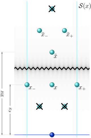
Figure 3. The strip $\mathcal{S}(x)$ centered at an atom $x\in\partial\mathcal{L}_{FS}$ of a crystalline configuration $D_{n}$ is depicted as an example of a strip containing all the elements $x,x_{\pm},\tilde{x},\tilde{x}_{\pm}$ with the possibility of the strip center $x$ and the strip top $\tilde{x}$ to coincide if $y_{M}=e_{S}$. The sites indicated by crossed atoms are sites of the planar lattice $\{x_{F}+k_{1}\bm{t}_{1}+k_{2}\bm{t}_{2}\,:\,\textrm{$k_{1},k_{2}\in\mathbb{Z}$}\}$ that surely are not in $D_{n}$ by definition of $\mathcal{L}_{F}$ and $\mathcal{S}(x)$.

In the following we refer to $x$ as the strip center of $\mathcal{S}(x)$, to $x_{\pm}$ as the strip lower (right and left) sides, to $\tilde{x}$ as the strip top, and to $\tilde{x}_{\pm}$ as the strip above (right and left) sides. Note that $x$ and $\tilde{x}$ coincide if $y_{M}=e_{S}$.

We define the strip energy associated to a strip $\mathcal{S}(x)$ by

$$E_{\rm strip}(x):=E_{\rm strip,below}(x)\,+\,E_{\rm strip,above}({\color[rgb]{0,0,0}x}),$$ (19)

where

$$E_{\rm strip,below}(x):= E_{\rm loc}(x)\,+\,\frac{1}{2}E_{\rm loc}(x_{+})\,+\,\frac{1}{2}E_{\rm loc}(x_{-})-c_{S}$$ (20)

in the case $\color[rgb]{0,0,0}q\neq 1\color[rgb]{0,0,0}$, while

$$E_{\rm strip,below}(x):= \frac{1}{2}E_{\rm loc}(x)\,+\,\frac{1}{4}E_{\rm loc}(x_{+})\,+\,\frac{1}{4}E_{\rm loc}(x_{-})-c_{S}$$ (21)

in the case $\color[rgb]{0,0,0}q=1\color[rgb]{0,0,0}$, and

$$E_{\rm strip,above}(x):=\begin{cases}E_{\rm loc}(\tilde{x})\,+\,w_{-}(\tilde{x})(E_{\rm loc}(\tilde{x}_{+})\,+\,w_{+}(\tilde{x})E_{\rm loc}(\tilde{x}_{-})&\textrm{if $\tilde{x}\neq x$,}\\ w_{-}(\tilde{x})E_{\rm loc}(\tilde{x}_{+})\,+\,w_{+}(\tilde{x})E_{\rm loc}(\tilde{x}_{-})&\textrm{if $\tilde{x}=x$}\end{cases}$$ (22)

with weights $w_{\pm}(\tilde{x})\in\color[rgb]{0,0,0}\{1/2,1\}$ given by

$$w_{\pm}(\tilde{x}):=\begin{cases}1&\textrm{if $x_{\pm}\not\in\color[rgb]{0,0,0}D_{n}\cap\partial\mathcal{L}_{FS}$ or \color[rgb]{0,0,0}$\tilde{x}_{\pm}\neq\widetilde{(x_{\pm})}_{\mp}$,}\\ \frac{1}{2}&\textrm{if $x_{\pm}\in\color[rgb]{0,0,0}D_{n}\cap\partial\mathcal{L}_{FS}$ and \color[rgb]{0,0,0}$\tilde{x}_{\pm}=\widetilde{(x_{\pm})}_{\mp}$}.\end{cases}$$ (23)

2.4. Almost-connected configurations

We recall from Section 2.1 that a configuration $D_{n}$ is said to be connected if every $x$ and $y$ in $D_{n}$ are connected through a path in the bonding graph of $D_{n}$, i.e., there exist $\ell\leq n$ and $x_{k}\in D_{n}$ for $k:=1,\dots,\ell$ such that $|x_{k}-x_{k-1}|=1$, $x_{1}=x$, and $x_{\ell}=y$, and we refer to maximal bonding subgraphs of $D_{n}$ connected through a path as connected components of $D_{n}$.

In order to treat the situation when $q\neq 1$ we need to introduce also a weaker notion of connectedness of configurations, which depends on $e_{S}$: We say that a configuration $D_{n}$ is almost connected if it is connected when $q=1$, and, if there exists an enumeration of its $k:=k_{D_{n}}$ connected components, say $D_{n}^{i}$, $i=1,\dots,k$, such that each $D_{n}^{i}$ is separated by at most $q$ from $\cup_{l=1}^{i-1}D_{n}^{l}$ for every $i=2,\dots,n$, when $q\neq 1$. We say that a family of connected components of $D_{n}$ form an almost-connected component of $D_{n}$ if their union is almost connected and, if $q\neq 1$, it is distant from all other components of $D_{n}$ by more than $q$.

Definition 2.1.

Given a configuration $D_{n}\in\mathcal{C}_{n}$, we define the transformed configuration $\mathcal{T}(D_{n})\in\mathcal{C}_{n}$ of $D_{n}$ as

$$\mathcal{T}(D_{n}):=\mathcal{T}_{2}(\mathcal{T}_{1}(D_{n})),$$

where $\mathcal{T}_{1}(D_{n})$ is the configuration resulting by iterating the following procedure, starting from $D_{n}$:

• If there are connected components without any activated bond with an atom of $\partial\mathcal{L}_{S}$, then select one of those components with lowest distance from $\partial\mathcal{L}_{S}$;

• Translate the component selected at the previous step of a vector in direction $-\bm{t}_{2}$ till either a bond with another connected component or with the substrate is activated.

(notice that the procedure ends when all connected components of $\mathcal{T}_{1}(D_{n})$ have at least a bond with $\partial\mathcal{L}_{S}$), and $\mathcal{T}_{2}(\mathcal{T}_{1}(D_{n}))$ is the configuration resulting by iterating the following procedure, starting from $\mathcal{T}_{1}(D_{n})$:

• If there are more than one almost-connected component, then select the almost-connected component whose leftmost bond with $\partial\mathcal{L}_{S}$ is the second (when compared with the other almost-connected components) starting from the left;

• Translate the almost-connected component selected at the previous step of a vector $-kq\bm{t}_{1}$ for some $k\in\mathbf{N}$ till, if $q=1$, a bond with another connected component is activated, or, if $q\neq 1$, the distance with another almost-connected component is less or equal to $q$;

(notice that the procedure ends when $\mathcal{T}_{2}(D_{n})$ is almost connected).

We notice that the transformed configuration $\mathcal{T}(D_{n})$ of a configuration $D_{n}\in\mathcal{C}_{n}$ satisfies the following properties:

• $\mathcal{T}(D_{n})$ is almost connected;

• Each connected component of $\mathcal{T}(D_{n})$ includes at least an atom bonded to $\partial\mathcal{L}_{S}$;

• $V_{n}(\mathcal{T}(D_{n}))\leq V_{n}(D_{n})$ (as no active bond of $D_{n}$ is deactivated by performing the transformations $\mathcal{T}_{1}$ and $\mathcal{T}_{2}$);

and, if $D_{n}$ is a minimizer of $V_{n}$ in $\mathcal{C}_{n}$, then

• $\mathcal{T}_{1}(D_{n}):=D_{n}$;

• $\mathcal{T}$ consists of translations of the almost-connected components of $D_{n}$ with respect to a vector (depending on the component) in the direction $-\bm{t}_{1}$ with norm in $\mathbb{N}\cup\{0\}$.

Finally we also observe that the definitions of $\mathcal{T}_{1}$, $\mathcal{T}_{2}$, and $\mathcal{T}$ are independent from $n$.

2.5. Continuum setting

For every set of finite perimeter $D\subset\mathbb{R}^{2}\setminus S$ we define its anisotropic surface energy $\mathcal{E}$ by

$$\mathcal{E}(D):=\int_{\partial^{*}D\cap\partial S}\Gamma(\nu_{D})d\mathcal{H}^{1}+\left(2c_{F}-\frac{c_{S}}{q}\right)\mathcal{H}^{1}(\partial^{*}D\cap\partial S)$$ (24)

where $\partial^{*}D$ denotes the reduced boundary of $D$ and the anisotropic surface tension $\Gamma:\mathbb{S}^{1}\to\mathbb{R}$ is the function such that it holds

$$\Gamma(\nu(\varphi))=2c_{F}\left(\nu_{2}(\varphi)-\frac{\nu_{1}(\varphi)}{\sqrt{3}}\right)$$ (25)

for every

$$\nu(\varphi)=\left(\begin{array}[]{c}-\sin\varphi\\ \cos\varphi\end{array}\right)\in\mathbb{S}^{1}\quad\text{with}\quad\varphi\in\left[0,\frac{\pi}{3}\right],$$

also when $\Gamma\circ\nu$ is extended periodically on $\mathbb{R}$ as a $\pi/3$-periodic function. Notice that $\Gamma(\bm{t}_{3})=\Gamma(\bm{t}_{2})=2c_{F}$. By extending $\Gamma$ by homogeneity we obtain a convex function, and in particular a Finsler norm on $\mathbb{R}^{2}$.

We also use the following auxiliary surface energy depending on $n$ in the proofs

$$\mathcal{E}_{n}(D):=\int_{\partial^{*}D\cap(\mathbb{R}^{2}\setminus\overline{S_{n}})}\Gamma(\nu_{D})d\mathcal{H}^{1}+\left(2c_{F}-\frac{c_{S}}{q}\right)\mathcal{H}^{1}(\partial^{*}D\cap\partial S_{n})$$ (26)

where

$$S_{n}:=S+\frac{e_{S}}{\sqrt{n}}\bm{t}_{3}.$$ (27)

2.6. Main results

In this section the rigorous statements of the main theorems of the paper are presented. We begin with following result that characterizes the wetting regime in terms of a condition only depending on $v_{FF}$ and $v_{FS}$, and the minimizers in such regime.

Theorem 2.2 (Wetting regime).

Let $D^{\rm w}_{n}:=\{w_{1},\dots,w_{n}\}\subset\partial\mathcal{L}_{FS}$ be any configuration such that, if $q=1$,

$$w_{i+1}:=w_{i}+\bm{t}_{1}$$ (28)

for every $i=1,\dots,{n}$ and every $n\in\mathbb{N}$. It holds that $D^{\rm w}_{n}$ satisfies the following two assertions for every $n\in\mathbb{N}$:

• $V_{n}(D^{\rm w}_{n})=\min{V_{n}(D_{n})}$,

• $V_{n}(D^{\rm w}_{n})<V_{n}(D_{n})$ for every crystalline configuration $D_{n}$ with $D_{n}\setminus\partial\mathcal{L}_{FS}\neq\emptyset$ (and, for the case $q=1$, also for every configuration $D_{n}$ with $D_{n}\setminus\partial\mathcal{L}_{FS}=\emptyset$ and for which (28) does not hold),

if and only if

$$\begin{cases}c_{S}\geq 6c_{F}&\text{if $q\neq 1$},\\ c_{S}\geq 4c_{F}&\text{if $q=1$}.\end{cases}$$ (29)

In particular, for the necessity of (29) it is enough assertion (i), and more specifically that there exists an increasing subsequence $(n_{k})_{k\in\mathbf{N}}$ such that $V_{n_{k}}(D^{\rm w}_{n_{k}})=\min{V_{n_{k}}(D_{n_{k}})}$ holds for every $n_{k}$.

We refer to (29) as a wetting condition or as the wetting regime, and to the opposite condition, namely

$$\begin{cases}c_{S}<6c_{F}&\textrm{if {\color[rgb]{0,0,0} $\color[rgb]{0,0,0}q\neq 1\color[rgb]{0,0,0}$}},\\ c_{S}<4c_{F}&\textrm{if {\color[rgb]{0,0,0} $\color[rgb]{0,0,0}q=1$}},\color[rgb]{0,0,0}\end{cases}$$ (30)

as the dewetting condition or the dewetting regime. The following result shows that connected components with the largest cardinality of minimizers incorporate the whole mass in the limit.

Theorem 2.3 (Mass conservation).

Assume (30). If $\widehat{D}_{n}$ are minimizers of $V_{n}$ among all crystalline configurations in $\mathcal{C}_{n}$, i.e.,

$$V_{n}(\widehat{D}_{n})=\min_{D_{n}\in\mathcal{C}_{n}}{V_{n}(D_{n})},$$

and we select for every $\widehat{D}_{n}$ a connected component $\widehat{D}_{n,1}\subset\widehat{D}_{n}$ with largest cardinality, then

$$\lim_{n\to\infty}{\mu_{\widehat{D}_{n}}(\widehat{D}_{n,1})}=1,$$

where $\mu_{\widehat{D}_{n}}$ are the empirical measure associated to $\widehat{D}_{n}$ defined by (12).

We rigorously prove by $\Gamma$-convergence that the discrete models converge to the continuum model, and in view of the previous result (even in the lack of a direct compactness result for general sequences of minimizers, possibly not almost connected), we prove convergence (up to passing to a subsequence and up to translations) of the minimizers of the discrete models to a bounded minimizer of the continuum model, which in turns it is also proven to exist.

Theorem 2.4 (Convergence of Minimizers).

Assume (30). The following statements hold:

• The functional

  $$E_{n}:=n^{-1/2}(I_{n}+6c_{F}n),$$ (31)

  where $I_{n}$ is defined by (LABEL:radon_functional), $\Gamma$-converges with respect to the weak* convergence of measures to the functional $I_{\infty}$ defined by

  $$I_{\infty}(\mu):=\begin{cases}\mathcal{E}(D_{\mu}),&\text{if \color[rgb]{0,0,0}there exists \color[rgb]{0,0,0}$D_{\mu}\subset\mathbb{R}^{2}\setminus S$ set of finite perimeter}\\ &\hskip 64.58313pt\text{with $|D_{\mu}|=1/\rho$ such that $\mu=\rho\chi_{D_{\mu}}$,}\\ +\infty,&\text{otherwise,}\\ \end{cases}$$ (32)

  for every $\mu\in\mathcal{M}(\mathbb{R}^{2})$, where $\rho:=2/\sqrt{3}$.

• The functional $I_{\infty}$ admits a minimizer in

  $$\mathcal{M}_{W}:=\bigg{\{}\mu\in\mathcal{M}(\mathbb{R}^{2})\ :\ \text{$\exists$ $D\subset\mathbb{R}^{2}\setminus S$}$$ set of finite perimeter, bounded

  $$\hskip 34.44434pt\text{with }|D|=\frac{1}{\rho}, \hskip 8.61108pt\text{ and such that $\mu=\rho\chi_{D}$}\bigg{\}}.$$ (33)

• Every sequence $\mu_{n}\in\mathcal{M}_{n}$ of minimizers of $E_{n}$ admits, up to translation in the direction $\bm{t}_{1}$ $($i.e., up to replacing $\mu_{n}$ with $\mu_{n}(\cdot+c_{n}\bm{t}_{1})$ for chosen fixed integers $c_{n}\in\mathbb{Z}$$)$, a subsequence converging with respect to the weak* convergence of measures to a minimizer of $I_{\infty}$ in $\mathcal{M}_{W}$.

Notice that the parameter $\rho:=2/\sqrt{3}$ in the definition of $\mathcal{M}_{W}$ is related to the fact that we chose the triangular lattice for $\mathcal{L}_{F}$, as $\rho$ is the density of atoms per unit volume of such lattice.

3. Wetting regime

In this section we single out conditions that entail wetting, i.e., the situation in which it is more convenient for film atoms to spread on the infinite substrate surface instead of accumulating in clusters, or islands, on top of it. In the following we refer to crystalline configurations $D^{\rm w}_{n}\subset\partial\mathcal{L}_{FS}$ as wetting configurations. We first consider the case $q\neq 1$.

Proposition 3.1.

Let $\color[rgb]{0,0,0}q\neq 1$ and $n\in\mathbb{N}$. Any wetting configuration $D^{\rm w}_{n}:=\{w_{1},\dots,w_{n}\}\subset\partial\mathcal{L}_{FS}$ satisfies the following two assertions:

• $V_{n}(D^{\rm w}_{n})=\min{V_{n}(D_{n})}$,

• $V_{n}(D^{\rm w}_{n})<V_{n}(D_{n})$ for any crystalline configuration $D_{n}$ with $D_{n}\setminus\partial\mathcal{L}_{FS}\neq\emptyset$,

if and only if

$$c_{S}\geq 6c_{F}.$$ (34)

Proof.

We begin by proving the sufficiency of (34) for the assertions (i) and (ii). Note that (i) easily follows from (ii) and the fact that any wetting configuration $D^{\rm w}_{n}$ has the same energy given by

$$V_{n}(D^{\rm w}_{n})=-c_{S}n.$$ (35)

In order to prove (ii) we proceed by induction on $n$. We first notice that (ii) is trivial for $n=1$. Then, we assume that (ii) holds true for every $k=1,\dots,n-1$ and prove that it holds also for $n$. Let $D_{n}$ be a crystalline configuration such that $D_{n}\setminus\partial\mathcal{L}_{FS}\neq\emptyset$. If $D_{n}\cap(\mathbb{R}\times\{r>e_{S}\})=\emptyset$, we can easily see that the energy of $D_{n}$ is higher of the energy of $D^{\rm w}_{n}$ at least by $c_{S}-2c_{F}$, which is positive by (34), since the elements in $D_{n}\setminus\partial\mathcal{L}_{FS}\neq\emptyset$ have at most two film bonds and no substrate bonds. Therefore, we can assume that $D_{n}\cap(\mathbb{R}\times\{r>e_{S}\})\neq\emptyset$. Let $L$ be the last line in $\mathbb{R}\times\{r>0\}$ parallel to $\bm{t}_{1}$ that intersects $D_{n}$ by moving upwards from $\mathbb{R}\times\{e_{S}\}$ (which exists since $D_{n}$ has a finite number of atoms).

We claim that

$$V_{n}(D_{n})\geq V_{n-\ell}(D_{n}\backslash L)-6c_{F}(\ell-1)-4c_{F},$$ (36)

where $\ell:=\#(D_{n}\cap L)$. We order the element of $D_{n}\cap L$ with increasing indexes with respect to $\bm{t}_{1}$, i.e., $D_{n}\cap L=\{x_{1},\dots,x_{\ell}\}$, and observe that $x_{1}$ has at most 3 bonds with film atoms in $D_{n}$ by construction, since $x_{1}$ is the leftmost element in $D_{n}\cap L$. We notice that in the same way, if $\ell>1$, every $x_{i}$ has at most 3 bonds with film atoms in $D_{n}\setminus\{x_{1},\dots,x_{i-1}\}$ for every $i=2,\dots,\ell-1$. Therefore, we obtain that

$$V_{n}(D_{n}) \geq V_{n-1}(D_{n-1}\backslash\{x_{1}\})-6c_{F}\geq V_{n-i}(D_{n-i}\backslash\{x_{1},\dots,x_{i}\})-6c_{F}i$$

$$\geq V_{n-(\ell-1)}(D_{n}\backslash\{x_{1},\dots,x_{\ell-1}\})-6c_{F}(\ell-1)\geq V_{n-\ell}(D_{n}\backslash L)-6c_{F}(\ell-1)-4c_{F},$$

which in turns is (36), where in the last inequality we used that $x_{\ell}$ has only at most 2 bonds with film atoms in $D_{n}\setminus L$, since $x_{\ell}$ is the rightmost element in $D_{n}\cap L$.

From (36) it follows that

$$V_{n}(D_{n}) \geq V_{n-\ell}(D_{n}\backslash L)-6c_{F}(\ell-1)-4c_{F}>V_{n-\ell}(D_{n}\backslash L)-6c_{F}\ell$$

$$>-c_{S}(n-\ell)-6c_{F}\ell\geq-c_{S}n,$$

where we used the induction and (35) in the third inequality, and (34) in the last inequality.

To prove the necessity of (34) notice that the Wulff configuration in $\mathbb{R}\times\{r>e_{s}\}$ has energy equal to $-6c_{F}n+C\sqrt{n}$ for some constant $C>0$. Therefore, from assertion (ii) and (35) it follows

$$\color[rgb]{0,0,0}-c_{S}n<\color[rgb]{0,0,0}-6c_{F}n+C\sqrt{n}.$$

After dividing by $n$ and letting $n\to\infty$ we obtain $c_{S}\geq 6c_{F}$.

∎

Remark 3.2.

Notice from the proof of Proposition 3.1 that for the necessity of (34) it is enough assertion (i) or, more precisely, it is enough that there exists an increasing subsequence $(n_{k})_{k\in\mathbf{N}}$ such that (i) holds for every $n_{k}$.

We now address the case $q=1$ for which we notice that $\partial\mathcal{L}_{FS}=\partial\mathcal{L}_{F}$.

Proposition 3.3.

Let $q=1$ and $n\in\mathbb{N}$. Any configuration $D^{\rm w}_{n}:=\{w_{1},\dots,w_{n}\}\subset\partial\mathcal{L}_{FS}$ such that

$$w_{i+1}:=w_{i}+\bm{t}_{1}$$ (37)

for every $i=1,\dots,{n}$, satisfies the following two assertions:

• $V_{n}(D^{\rm w}_{n})=\min{V_{n}(D_{n})}$,

• $V_{n}(D^{\rm w}_{n})<V_{n}(D_{n})$ for any crystalline configuration $D_{n}$ such that either $D_{n}\setminus\partial\mathcal{L}_{FS}\neq\emptyset$ or not satisfying (37),

if and only if

$$c_{S}\geq 4c_{F}.$$ (38)

Proof.

The proof is based on the same arguments employed for Proposition 3.1 and on the following observations. Any wetting configuration $D^{\rm w}_{n}$ satisfying (37) has the same energy given by

$$V_{n}(D^{\rm w}_{n})=-c_{S}n-2c_{F}(n-1).$$ (39)

In order to prove the sufficiency of (38) for assertion (ii) (assertion (i) follows in view of (39)), we can restrict also in this case without loss of generality to configurations $D_{n}\cap(\mathbb{R}\times\{r>e_{S}\})\neq\emptyset$, since any wetting configuration that does not satisfy (37) has energy obviously higher than (39) (because $n-1$ is the maximum number of bonds in $\partial\mathcal{L}_{F}$).

In order to prove the necessity of (38) for assertions (i) and (ii), we again consider the Wulff shape with $n$ atoms in $\mathbb{R}\times\{r>e_{s}\}$ which has energy $-6c_{F}n+C\sqrt{n}$ for some constant $C>0$, and observe that

$$-c_{S}n-2c_{F}(n-1)<-6c_{F}n+C\sqrt{n}$$

by assertion (ii) and (39).

∎

Remark 3.4.

Notice from the proof of Proposition 3.3 that for the necessity of (38) it is enough assertion (i) or, more precisely, it is enough that there exists an increasing subsequence $(n_{k})_{k\in\mathbf{N}}$ such that (i) holds for every $n_{k}$.

We refer to (34) and (38) as wetting conditions. Condition (38) is weaker than (34) because if $q=1$, then film atoms of wetting configurations can be bonded to the two film atoms at their sides in $\partial\mathcal{L}_{FS}$ (if filled) besides to their corresponding substrate atom, and Proposition 3.3 show that such configuration are preferable. We notice that the same arguments used in Propositions 3.1 and 3.3 work for other rigid positioning of $\mathcal{L}_{F}$ and $\mathcal{L}_{S}$. For example for the case with

$$e_{S}:=\frac{3}{4}\qquad\text{ and}\qquad x_{F}:=\left(-\frac{1}{8},\frac{1}{8}\sqrt{35}\right)$$

the wetting condition (34) is replaced by $c_{S}\geq 5c_{F}$, since film atoms in wetting configurations may present a film bond besides the substrate bond.

Proof of Theorem 2.2.

The assertion directly follows from Proposition 3.1 and Proposition 3.3 for the case $q\neq 1$ and the case $q=1$, respectively. ∎

4. Compactness

In the remaining part of the paper we work in the dewetting regime, i.e., under the assumption (30). We begin by establishing a lower bound in terms of $c_{F}$ and $c_{S}$ of the strip energy $E_{\rm strip}(x)$ uniform for every $x\in D_{n}\cap\partial\mathcal{L}_{F}$. To this aim, we need to distinguish the case $q=1$ from $q\neq 1$ as already done in Section 3 because of the different contributions in $E_{\rm strip}(x)$ of the substrate interactions.

Lemma 4.1.

We have that

$$E_{\rm strip}(x)\geq\Delta_{\rm strip}$$

with

$$\Delta_{\rm strip}:=\begin{cases}6c_{F}-c_{S},&\text{if $\color[rgb]{0,0,0}q\neq 1\color[rgb]{0,0,0}$,}\\ 4c_{F}-c_{S},&\text{if $\color[rgb]{0,0,0}q=1\color[rgb]{0,0,0}$},\end{cases}$$ (40)

for every $x\in D_{n}\cap\partial\mathcal{L}_{F}$.

Proof.

Fix $x\in D_{n}\cap\partial\mathcal{L}_{F}$. We begin by observing that the strip center $x$ surely misses the bonds with the atoms missing at the 2 positions $x-\bm{t}_{2}+k\bm{t}_{1}$ for $k=0,1$ as shown in Figure 3. Furthermore, either $x$ misses the bond with $x_{-}$ or $x_{-}\in{\color[rgb]{0,0,0}D_{n}}$ and $x_{-}$ misses the bonds with the 2 positions $x-\bm{t}_{2}+k\bm{t}_{1}$ for $k=-1,0$ (which in the strip energy are counted with half weights). We can reason similarly for $x_{+}$. Therefore, by the definition of energy of the low strip $E_{\rm strip,below}$,

$$E_{\rm strip,below}\color[rgb]{0,0,0}\geq\color[rgb]{0,0,0}\begin{cases}4c_{F}-c_{S},&\text{if $q\neq 1$,}\\ 2c_{F}-c_{S},&\text{if $q=1$,}\end{cases}$$

We analyze $E_{strip,above}$. There are several possibilities:

1. neither of $\tilde{x}_{+}$ and $\tilde{x}_{-}$ belongs to $D_{n}$;

2. exactly one of $\tilde{x}_{+}$ and $\tilde{x}_{-}$ belongs to $D_{n}$;

3. both $\tilde{x}_{+}$ and $\tilde{x}_{-}$ belong to $D_{n}$.

In case of (1) we have the contribution of $2c_{F}$ since $\tilde{x}$ misses two bonds. In case of (3) each of $\tilde{x}_{+}$ and $\tilde{x}_{-}$ misses at least one bond (namely with $\tilde{x}+2\bm{t}_{2}-\bm{t}_{1}$ which is not in $D_{n}$ due to the definition of $\tilde{x}$). If $\tilde{x}_{\pm}\neq\widetilde{(x_{\pm})}_{\mp}$ we have the energy contribution of at least $2c_{F}$. On the other hand if it is valid that $\tilde{x}_{\pm}=\widetilde{(x_{\pm})}_{\mp}$, we have the energy contribution of $c_{F}$ due to the missing bond with $\tilde{x}+2\bm{t}_{2}-\bm{t}_{1}$ and each of $\tilde{x}_{\pm}$ misses one more bond (namely with $\tilde{x}+2\bm{t}_{2}$ and $\tilde{x}+2\bm{t}_{2}-2\bm{t}_{1}$, which in this case do not belong to $D_{n}$). The similar analysis can be made if $\tilde{x}_{+}=\widetilde{(x_{+})}_{-}$ or $\tilde{x}_{-}=\widetilde{(x_{-})}_{+}$. Thus we have again energy defficiency of $2c_{F}$. Finally in the case of (ii) without loss of generality we assume that $\tilde{x}_{+}\in D_{n}$. $\tilde{x}$ is already missing one bond (one $c_{F}$) and again one bond of $\tilde{x}_{+}$ is missing since $\tilde{x}+2\bm{t}_{2}-\bm{t}_{1}$ is not in $D_{n}$. Again, this bond is counted as one $c_{F}$, if $\tilde{x}_{+}\neq\widetilde{(x_{+})}_{-}$ and as $c_{F}/2$, if $\tilde{x}_{+}\neq\widetilde{(x_{+})}_{-}$. In this case one more $c_{F}/2$ we obtain since $\tilde{x}_{+}$ is missing one bond with $\tilde{x}+2\bm{t}_{2}$.

Therefore, in the strip energy $E_{\rm strip}$ the terms related to the triple $\tilde{x}$, $\tilde{x}_{+}$, and $\tilde{x}_{-}$ give a contribution of at least $2c_{F}$.

∎

We now observe that the energy $V_{n}(D_{n})$ of any crystalline configuration $D_{n}$ is bounded below by $-6c_{F}n$ plus a positive deficit due to the boundary of $D_{n}$ where atoms have less than 6 film bonds and could have a bond with the substrate.

Lemma 4.2.

If (30) holds, then there exists $\Delta>0$ such that

$$V_{n}(D_{n})\geq-6c_{F}n\,+\,\Delta\#\partial D_{n}$$ (41)

for every crystalline configuration $D_{n}\subset\mathcal{L}_{F}$. Furthermore, the following two assertions are equivalent:

• There exists a constant $C>0$ such that $\#\partial D_{n}\leq C\sqrt{n}$ for every $n\in\mathbb{N}$,

• There exists a constant $C^{\prime}>0$ such that $E_{n}(\mu_{D_{n}})\leq C^{\prime}$ for every $n\in\mathbb{N}$.

Proof.

We begin by observing that from (16) and (19) it follows that

$$6c_{F}n\,+\,V_{n}(D_{n})\, =\,\sum_{x\in D_{n}}\left(\sum_{y\in{\color[rgb]{0,0,0}D_{n}}\setminus\{x\}}v_{FF}(|x-y|)+6c_{F}\right)\,+\,\sum_{x\in D_{n}}v^{1}(x)$$

$$=\,\sum_{x\in D_{n}}E_{\rm loc}(x)\,+\,\sum_{x\in D_{n}}v^{1}(x)$$

$$\geq\,\sum_{x\in D_{n}\cap{\color[rgb]{0,0,0}\partial\mathcal{L}_{FS}}}E_{\rm strip}(x)\,+\,\sum_{x\in D_{n}\setminus\mathcal{S}({\color[rgb]{0,0,0}\partial\mathcal{L}_{FS}})}E_{\rm loc}(x),$$ (42)

where

$$\mathcal{S}(\partial\mathcal{L}_{FS})=\mathcal{S}_{\color[rgb]{0,0,0}D_{n}\color[rgb]{0,0,0}}({\color[rgb]{0,0,0}\partial\mathcal{L}_{FS}}):=\{y\in\mathcal{S}(x)\,:\,x\in D_{n}\cap{\color[rgb]{0,0,0}\partial\mathcal{L}_{FS}}\},$$ (43)

because $v^{1}(x)=0$ for every $x\in D_{n}\setminus\partial\mathcal{L}_{FS}$ and the careful choice of the weights in (20), (21), and (22) with (23). More precisely, we notice that for every point in $D_{n}\cap{\color[rgb]{0,0,0}\partial\mathcal{L}_{FS}}$ the local energy $E_{\rm loc}(x)$ is counted at most once. The weights $c_{\pm}(\tilde{x}_{\pm})$ are instead chosen so that the local energy of $\tilde{x}_{\pm}$ is fully counted if $\tilde{x}_{\pm}$ do not belong to the next strip and only half in the other case. Thus these weights are also at most one. We now observe that

$$\sum_{x\in D_{n}\setminus\mathcal{S}(\color[rgb]{0,0,0}\partial\mathcal{L}_{FS}\color[rgb]{0,0,0})}E_{\rm loc}(x)\geq c_{F}\#(\partial D_{n}\setminus\mathcal{S}({\color[rgb]{0,0,0}\partial\mathcal{L}_{FS}}))$$ (44)

because every point in $D_{n}\setminus\mathcal{S}(\partial\mathcal{L}_{FS})$ has 6 bonds if not on the $\partial D_{n}$ where at least one bond is missing by definition.

Therefore, by (42), (44), and Lemma 4.1 we obtain that

$$6c_{F}n\,+\,V_{n}(D_{n})\, \geq\,\sum_{x\in D_{n}\cap{\color[rgb]{0,0,0}\partial\mathcal{L}_{FS}}}E_{\rm strip}(x)\,+\,\sum_{x\in D_{n}\setminus\mathcal{S}({\color[rgb]{0,0,0}\partial\mathcal{L}_{FS}})}E_{\rm loc}(x),$$

$$\geq\Delta_{strip}\#(D_{n}\cap{\color[rgb]{0,0,0}\partial\mathcal{L}_{FS}})\,+\,c_{F}\#(\partial D_{n}\setminus\mathcal{S}({\color[rgb]{0,0,0}\partial\mathcal{L}_{FS}}))$$

$$\geq\min\left\{\frac{\Delta_{strip}}{6},c_{F}\right\}\#\partial D_{n}$$ (45)

where in the last inequality we used that $\color[rgb]{0,0,0}\#\mathcal{S}(\partial\mathcal{L}_{FS})\leq 6\#D_{n}\cap\partial\mathcal{L}_{FS}\color[rgb]{0,0,0}$. The assertion now easily follows from (45) by choosing

$$\Delta:=\min\left\{\frac{\Delta_{strip}}{6},c_{F}\right\}>0,$$

where we used (30).

To prove the last assertion we observe that assertion (i) implies (ii) since by (15) and (31)

$$\sqrt{n}E_{n}(\mu_{D_{n}})=V_{n}(D_{n})+6c_{F}n\leq 6c_{F}\#\partial D_{n},$$

where in the last equality we used the definition of $\partial D_{n}$. Furthermore, also by (41),

$$\Delta\#\partial D_{n}\leq V_{n}(D_{n})+6c_{F}n=\sqrt{n}E_{n}(\mu_{D_{n}})$$

and hence, assertion (ii) implies (i).

∎

In view of the previous lower bound for the energy of a configuration $D_{n}$ we are now able to prove a compactness results. We notice that to achieve compactness the negative contribution coming at the boundary from the interaction with the substrate needs to be compensated. This is not trivial, e.g., in the case $6c_{F}>c_{S}>4c_{F}$, where atoms $x$ of configurations on $\partial\mathcal{L}_{FS}$ have one bond with a substrate atom and at least two bonds with film atoms missing. A way to solve the issue is to look for extra positive contributions from other atoms in the boundary. However, just looking for neighboring atoms might be not enough, e.g., in the case with $e_{S}=2$ or $e_{S}=\frac{2}{3}$. The issue is solved in the proof of the following compactness result by introducing a new non-local argument called the strip argument that involve looking at the whole strip $\mathcal{S}(x)$. The same argument would work for other rigid positioning of $\mathcal{L}_{F}$ and $\mathcal{L}_{S}$, such as for

$$e_{S}:=\frac{3}{4}\qquad\text{ and}\qquad x_{F}:=\left(-\frac{1}{8},\frac{1}{8}\sqrt{35}\right).$$

We conclude the section with compactness results for sequences of almost-connected configuration (see Section 2.4 for the definition). We remind the reader that by the trasformation defined in Definition 2.1 for any configuration $D_{n}$ there exists the almost-connected configuration $\widetilde{D}_{n}$ such that $V_{n}(\widetilde{D}_{n})\leq V_{n}(D_{n})$.

Proposition 4.3.

Assume that (30) holds. Let $D_{n}\in\mathcal{C}_{n}$ be almost-connected configurations such that

$$V_{n}(D_{n})\leq-6c_{F}n+Cn^{1/2}$$ (46)

for a constant $C>0$. Then there exist an increasing sequence $n_{r}$, $r\in\mathbb{N}$, and a measure $\mu\in\mathcal{M}(\mathbb{R}^{2})$ with $\mu\geq 0$ and $\mu(\mathbb{R}^{2})=1$ such that $\mu_{r}\rightharpoonup^{*}\mu$ in $\mathcal{M}(\mathbb{R}^{2})$, where $\mu_{r}:=\mu_{D_{n_{r}}\color[rgb]{0,0,0}(\,\cdot\,+a_{n_{r}})}$ for some translations $a_{n}\in\mathbb{R}^{2}$ (see (12) for the definition of the empirical measures $\mu_{D_{n_{r}}}$). Moreover, if $D_{n}\in\mathcal{C}_{n}$ are minimizers of $V_{n}$ in $\mathcal{C}_{n}$, then we can choose $a_{n}=t_{n}\bm{t}_{1}$ for integers $t_{n}\in\mathbb{Z}$.

Proof.

In the following we denote by $B(x,R)$ an open ball of radius $R>0$ centered at $x\in\mathbb{R}^{2}$ and we define $B(R):=B(o,R)$ where $o$ is the origin in $\mathbb{R}^{2}$. We want to show that there exists $R>0$ such that $D_{n}\subset B(R)$ (up to a translation) for every $n$.

To this aim we denote for any $D_{n}$ its $k:=k_{D_{n}}$ connected components by $D_{n}^{i}$ for $\color[rgb]{0,0,0}i\color[rgb]{0,0,0}=1,\dots,k$. We define the sets

$$\color[rgb]{0,0,0}\Omega_{i}:=\bigcup_{x\in D_{n}^{i}}\nu_{\textrm{trunc}}(x),$$

for $i=1,\dots,k$, where

$$\nu_{\textrm{trunc}}(x):=\nu(x)\cap B(x,q)$$

with $q$ defined in (11) and $\nu(x)$ denoting the (closed) Voronoi cell associated to $x$ with respect to $D_{n}^{i}$, i.e.,

$$\nu(x):=\{y\in\mathbb{R}^{2}\ :\ \text{$|y-x|\leq|y-x^{\prime}|$ for all $x^{\prime}\in D_{n}^{i}\setminus\{x\}$}\},\color[rgb]{0,0,0}$$ (47)

and we observe that by construction and the convexity of $\nu(x)$,

$$|\partial\nu_{\textrm{trunc}}(x)|\leq 2\color[rgb]{0,0,0}q\pi.$$ (48)

We claim that $\Omega_{i}$ are connected. Indeed, if $x,y\in D_{n}$ are such that $|x-y|=1$, then it is easily seen that the midpoint on the line that connects $x$ and $y$ belongs to both $\nu(x)\cap\nu(y)$ and $B(x,q)\cap B(y,q)$. The second claim easily follows from (11) while the first claim follows from the triangular inequality (it is impossible that for every $z\in D_{n}$ it is valid

$$\left|z-\frac{x+y}{2}\right|<1/2$$

since then by the triangular inequality $z$ would be distant from both $x$ and $y$ less than one).

We now claim that also

$$\Omega:=\bigcup_{x\in D_{n}}\nu_{\textrm{trunc}}(x),$$

is connected. This follows by showing that $\Omega_{i}$ and $\cup_{i=1}^{i-1}\color[rgb]{0,0,0}\Omega_{l}$ are connected for $i=2,\dots,k$, which in turns is a consequence of the fact that by definition $D_{n}^{i}$ is separated by at most $q$ from $\cup_{l=1}^{i-1}\color[rgb]{0,0,0}D_{n}^{l}$ for $i=2,\dots,k$. In fact, by the same reasoning used in the previous claim applied this time to two points $x\in D_{n}^{i}$ and $y\in\cup_{l=1}^{i-1}D_{n}^{l}$ chosen such that $|x-y|=\textrm{dist}(D_{n}^{i},\cup_{l=1}^{i-1}D_{n}^{l})$, where $\textrm{dist}(A,B)$ with respect to two subsets $A$ and $B$ of $\mathbb{R}^{2}$ denotes the distance between them, we can deduce that $(x+y)/2$ belongs to both $\nu(x)\cap\nu(y)$ and $B(x,q)\cap B(y,q)$, which yields the claim.

Therefore, we have that

$$\textrm{diam}(D_{n}):=\max_{x,y\in D_{n}}|x-y|\leq\textrm{diam}(\Omega)\leq\frac{1}{2}|\partial\Omega|\leq\frac{1}{2}\sum_{x\in\partial D_{n}}|\partial\nu_{\textrm{trunc}}(x)|\leq\pi\color[rgb]{0,0,0}q\#\partial D_{n}$$ (49)

where $\textrm{diam}(A)$ of a set $A$ is the diameter of $A$ and we used that $\Omega$ is connected in the second inequality, that if $x\in D_{n}$ has $6$ film neighbors, then by elementary geometric observation $\nu_{\textrm{trunc}}(x)\cap\partial\Omega=\emptyset$ in the third inequality, and (48) in the last inequality.

Finally, from (46), (49) and Lemma 4.2 we obtain that

$$\textrm{diam}(D_{n})\leq\frac{C\pi\color[rgb]{0,0,0}q}{\Delta}n^{1/2}$$

and hence, by (12) there exist translations $\mu_{n}$ of $\mu_{D_{n}}$ such that $\textrm{supp}\mu_{n}\subset B(R)$ for some $R>C\pi q/2\Delta$ and for every $n$. Therefore, since $|\mu_{D_{n}}|(\mathbb{R}^{2})=1$ for every $n$, by [1, Theorem 1.59] there exist a subsequence $(n_{r})_{r}\in\mathbf{N}$ and a measure $\mu\in\mathcal{M}(\mathbb{R}^{2})$ such that $\mu_{r}\stackrel{{\scriptstyle*}}{{\rightharpoonup}}\mu$ in $\mathcal{M}(\mathbb{R}^{2})$. Furthermore, $\mu\geq 0$ and

$$\mu(\mathbb{R}^{2})\leq\lim_{r\to\infty}{\mu}_{r}(\mathbb{R}^{2})=1.$$

In order to conclude the proof it suffices to prove that $\mu(\mathbb{R}^{2})=1$, and this directly follows from the fact that the support of $\mu_{r}$ are contained in a compact set of $\mathbb{R}^{2}$. ∎

The following compactness result is the analogous of [3, Theorem 1.1] in our setting with substrate interactions.

Theorem 4.4 (Compactness).

Assume (30). Let $D_{n}\in\mathcal{C}_{n}$ be configurations satisfying (46) and let $\mu_{n}:=\mu_{\mathcal{T}(D_{n})}$ be the empirical measures associated to the transformed configurations $\mathcal{T}(D_{n})\in\mathcal{C}_{n}$ associated to $D_{n}$ by Definition 2.1. Then, up to translations $($i.e., up to replacing $\mu_{n}$ by $\mu_{n}(\cdot+a_{n})$ for some $a_{n}\in\mathbb{R}^{2}$$)$ and a passage to a non-relabelled subsequence, $\mu_{n}$ converges weak* in $\mathcal{M}(\mathbb{R}^{2})$ to a measure $\mu\in\mathcal{M}_{W}$, where $\mathcal{M}_{W}$ is defined in (33). Furthermore, if $D_{n}\in\mathcal{C}_{n}$ are minimizers of $V_{n}$ in $\mathcal{C}_{n}$, then we can choose $a_{n}=t_{n}\bm{t}_{1}$ for integers $t_{n}\in\mathbb{Z}$.

Proof.

We begin by observing that the transformed configurations $\mathcal{T}(D_{n})$ of the configurations $D_{n}$ are almost-connected configurations in $\mathcal{C}_{n}$ since they result from applying transformation $\mathcal{T}_{2}$, and that

$$V_{n}(\mathcal{T}(D_{n}))\leq V_{n}(D_{n}),$$ (50)

since no active bond of $D_{n}$ is deactivated by performing the transformations $\mathcal{T}_{1}$ and $\mathcal{T}_{2}$ (see Definition 2.1 for the definition of $\mathcal{T}_{1}$ and $\mathcal{T}_{2}$). Therefore, in view of Proposition 4.3 by (46) and (50) we obtain that, up to a non-relabeled subsequence, there exist $a_{n}\in\mathbb{R}^{2}$ and a measure $\mu\in\mathcal{M}(\mathbb{R}^{2})$ with $\mu\geq 0$ and $\mu(\mathbb{R}^{2})=1$ such that

$$\mu_{\mathcal{T}(D_{n})}(\cdot+a_{n})\rightharpoonup^{*}\mu$$

in $\mathcal{M}(\mathbb{R}^{2}).$ We can then conclude that $\mu\in\mathcal{M}_{W}$ by directly applying the arguments in the proof of [3, Theorem 1.1].

∎

We notice that, if the sequence $D_{n}\in\mathcal{C}_{n}$ is a sequence of almost-connected configurations, then Theorem 4.4 directly holds for $D_{n}$ without the need to pass to the associated transformed configurations $\mathcal{T}(D_{n})$ given by Definition 2.1.

5. Lower bound

We denote by $h_{1/\sqrt{3}}(x)$ the interior part of the Voronoi cell associated to every $x\in\mathcal{L}_{F}$ with respect to $\mathcal{L}_{F}$, i.e.,

$$h_{1/\sqrt{3}}(x):=\left\{y\in\mathbb{R}^{2}\ :\ \text{$|y-x|<|y-x^{\prime}|$ for all $x^{\prime}\in\mathcal{L}_{F}\setminus\{x\}$}\right\}$$

that is an open hexagon of radius $1/\sqrt{3}$, and by $v(x)$ its scaling in $\mathcal{L}_{F}/\sqrt{n}$, i.e.

$$v(x):=\frac{h_{1/\sqrt{3}}(x)}{\sqrt{n}}.$$ (51)

Given a configuration $D_{n}$, we consider the auxiliary set $H_{n}$ associated to $D_{n}$ which was introduced in [3] and defined by

$$H_{n}=\bigcup_{x\in D_{n}}\overline{v(x)}.$$ (52)

The boundary of $H_{n}$ is given by the union of a number $M\in\mathbb{N}$ (depending on $D_{n}$) of closed polygonal boundaries $P_{1},\dots,P_{M}$. For $k=1,\dots,M$ we denote the $m_{k}\in\mathbb{N}$ vertices of $P_{k}$ by $v_{1}^{k},\dots,v_{m_{k}}^{k}$ and we set $v_{m_{k}+1}^{k}:=v_{1}^{k}$, so that

$$P_{k}:=\bigcup_{i=1}^{m_{k}}[v_{i+1}^{k},v_{i}^{k}]$$

where $[a,b]$ denotes the closed segment with endpoints $a,b\in\mathbb{R}^{2}$. Notice that each $m_{k}$ is even and that we can always order the vertices so that

$$v_{2i}^{k}\in V_{\mathcal{L}_{F}}^{\rm e}:=\left(\frac{1}{3\sqrt{n}}(\bm{t}_{1}+\bm{t}_{2})+\frac{1}{\sqrt{n}}\mathcal{L}_{F}\right)$$

and

$$v_{2i-1}^{k}\in V_{\mathcal{L}_{F}}^{\rm o}:=\left(\frac{1}{3\sqrt{n}}(2\bm{t}_{1}-\bm{t}_{2})+\frac{1}{\sqrt{n}}\mathcal{L}_{F}\right)$$

(see Figure 4). To avoid the atomic-scale oscillations in $\partial H_{n}$ between the two sets of vertices $V_{\mathcal{L}_{F}}^{\rm e}$ and $V_{\mathcal{L}_{F}}^{\rm o}$, we introduce another auxiliary set denoted by $H^{\prime}_{n}$ where such oscillations are removed, by considering only the vertices in one of the two sets, say $V_{\mathcal{L}_{F}}^{\rm o}$ as depicted in Figure 4. More precisely, the set $H^{\prime}_{n}\subset\mathbb{R}^{2}$ is defined as the unique set with $D_{n}\subset H_{n}^{\prime}$ such that

$$\partial H_{n}^{\prime}:=\bigcup_{k=1}^{M}P_{k}^{\prime},$$ (53)

where

$$P_{k}^{\prime}:=\bigcup_{i=1}^{m_{k}/2}[v_{2i-1}^{k},v_{2i+1}^{k}].$$

Figure 4. A configuration $D_{n}$ is depicted with scaled Voronoi cells $v(x)$ for every $x\in D_{n}$. The boundary of $H_{n}$, which in this example consists of two polygonal lines (one “internal” and one “external”), is indicated with a dashed black line while the boundary of $H_{n}^{\prime}$ with a continuous red line.

It easily follows from the construction of the auxiliary sets $H_{n}$ and $H_{n}^{\prime}$ associated to the configuration $D_{n}$ that

$$|H_{n}\Delta H_{n}^{\prime}|\leq\frac{\#\partial D_{n}}{8\color[rgb]{0,0,0}n\color[rgb]{0,0,0}\sqrt{3}},$$ (54)

and

$$\left|\color[rgb]{0,0,0}\mathcal{H}^{1}(\partial H_{n})\color[rgb]{0,0,0}-\color[rgb]{0,0,0}\mathcal{H}^{1}(\partial H_{n}^{\prime})\color[rgb]{0,0,0}\right|\leq 2\sqrt{3}\frac{\#\partial D_{n}}{\sqrt{n}}.$$ (55)

In the following we use the notation

$$\partial\mathcal{L}_{FS}^{n}:=\frac{\partial\mathcal{L}_{FS}}{\sqrt{n}}.$$

For every point $y\in\partial\mathcal{L}_{FS}^{n}$ we denote its left and right half-open intervals with length $1/\sqrt{n}$ by

$$\color[rgb]{0,0,0}I^{+}_{y}:=\left[y,y+\frac{1}{2\sqrt{n}}\right)\quad\textrm{and}\quad I^{-}_{y}:=\left(y-\frac{1}{2\sqrt{n}},y\right],$$

respectively, and we define the oscillatory sets of $y\in\partial\mathcal{L}_{FS}^{n}$ by

$$O_{n}^{y}:=O_{n}^{y,-}\cup O_{n}^{y,+},$$

where $O_{n}^{y,\pm}$ are the left and right oscillatory sets of $y\in\partial\mathcal{L}_{FS}^{n}$, i.e.,

$$\color[rgb]{0,0,0}O_{n}^{y,\pm}:=\{I^{\pm}_{y}\times\mathbb{R}:y\in\partial\mathcal{L}_{FS}^{n}\}$$

(see Figure 2). The (overall) oscillatory set $O_{n}$ is defined as

$$O_{n}:=\bigcup_{y\in\partial\mathcal{L}_{FS}^{n}}O_{n}^{y}.$$ (56)

Here $O_{n}$ is the oscillatory set on that consists of union of stripes of width $1/\sqrt{n}$ and infinite length (following the way of construction of the set $H_{n}^{\prime}$) that correspond to the possible positions of film atoms at the place $x_{2}=\frac{e_{S}}{\sqrt{n}}$ that are at distance $\frac{e_{S}}{\sqrt{n}}$ from some of substrate atoms. $\nu_{H_{n}^{\prime}}$ is a normal at the boundary.

The following lemma will help in the proof of lower-semicontinuity result. It is a simplified version of the proof of [3, Theorem 1.1] and we give it for the sake of completeness. We recall that $\rho:=2/\sqrt{3}$.

Lemma 5.1.

Let $D_{n}\in\mathcal{C}_{n}$ be such that $E_{n}(\mu_{D_{n}})$ is bounded, where $\mu_{D_{n}}$ is the empirical measure associated with $D_{n}$. Let $H_{n}^{\prime}$ be defined as above. Then we have that $\mu_{D_{n}}-\rho\chi_{H_{n}^{\prime}}\stackrel{{\scriptstyle*}}{{\rightharpoonup}}0$.

Proof.

It is easy to see that

$$\mu_{D_{n}}-\rho\chi_{H_{n}}\stackrel{{\scriptstyle*}}{{\rightharpoonup}}0.$$

Namely for $\psi\in C_{0}(\mathbb{R}^{2})$, where $C_{0}(\mathbb{R}^{2})$ denotes the set of continuous functions with compact support in $\mathbb{R}^{2}$, we have that

$$\left|\int_{\mathbb{R}^{2}}(\psi d\mu_{D_{n}}-\rho\chi_{H_{n}}\psi)dx\right|\leq\frac{1}{n}\sum_{x\in D_{n}}\sup_{x\in D_{n}}\{|\psi(x)-\psi(y)|:|x-y|\leq\frac{1}{\sqrt{3n}}\}\\ \to 0,$$

as $n\to\infty$. From estimate (54) and Lemma 4.2 we have that $\rho\chi_{H_{n}}-\rho\chi_{H_{n}^{\prime}}\to 0$ strongly in $L^{1}$, from which we have the claim. ∎

The following lower-semicontinuity result for the discrete energies $E_{n}$ is based on adapting some ideas used in [2] and [16].

Theorem 5.2.

If $\{D_{n}\}$ is a sequence of configurations such that

$$\mu_{D_{n}}\stackrel{{\scriptstyle*}}{{\rightharpoonup}}\rho\chi_{\color[rgb]{0,0,0}D\color[rgb]{0,0,0}}$$

weakly* with respect to the convergence of measures, where $\mu_{D_{n}}$ are the associated empirical measures of $D_{n}$ and $D\subset\mathbb{R}^{2}\setminus S$ is a set of finite perimeter with $|D|=1/\rho$, then

$$\liminf_{n\to\infty}E_{n}(\mu_{D_{n}}) \geq \mathcal{E}(D).$$ (57)

Proof.

Let $\{D_{n}\}\subset\mathcal{C}_{n}$ be a sequence of configurations such that $\mu_{D_{n}}\stackrel{{\scriptstyle*}}{{\rightharpoonup}}\rho\chi_{E}$ weakly* with respect to the convergence of measures, for a set $E\subset\mathbb{R}^{2}\setminus S$ of finite perimeter with $|E|=\sqrt{3}/2$. We focus on the case $q\neq 1$ only, since the other case is simpler.

Without loss of generality we can assume that the limit in the left hand side of (57) is reached and it is finite, and hence there exists $C>0$ such that $E_{n}(\mu_{D_{n}})\leq C$ for every $n\in\mathbb{N}$. Then, by the second assertion of Lemma 4.2 there exists $C^{\prime}>0$ such that $\#\partial D_{n}\leq C^{\prime}\sqrt{n}$ for every $n\in\mathbb{N}$, from which it follows that there exists a constant $C^{\prime\prime}>0$ such that

$$\mathcal{H}^{1}(\partial H_{n}^{\prime})<C^{\prime\prime}$$ (58)

for every $n\in\mathbb{N}$. Therefore, by, e.g., Corollary 7.5, up to a non-relabelled subsequence, $\rho\chi_{H_{n}^{\prime}}$ weakly converges in $SBV_{\textrm{loc}}(\mathbb{R}^{2})$ to a function $g\in SBV_{\textrm{loc}}(\mathbb{R}^{2})$. Since, up to extracting an extra non-relabelled subsequence, $\mu_{D_{n}}-\rho\chi_{H_{n}^{\prime}}\stackrel{{\scriptstyle*}}{{\rightharpoonup}}0$ as proved in Lemma 5.1 and $\mu_{D_{n}}\stackrel{{\scriptstyle*}}{{\rightharpoonup}}\rho\chi_{E}$ by hypothesis, then $g:=\rho\chi_{E}$ and $\rho\chi_{H_{n}^{\prime}}\stackrel{{\scriptstyle*}}{{\rightharpoonup}}\rho\chi_{E}$.

We observe that by (15), (31), and (53) we have that

$$E_{n}(\mu_{D_{n}})=2c_{F}\mathcal{H}^{1}(\partial H_{n}^{\prime})-c_{S}\mathcal{H}^{1}\left(\partial H_{n}^{\prime}\cap\left(\mathbb{R}\times\left\{\frac{e_{S}}{\sqrt{n}}-\frac{1}{2\color[rgb]{0,0,0}\sqrt{3n}\color[rgb]{0,0,0}}\right\}\right)\cap O_{n}\right)$$ (59)

where $O_{n}$ is the oscillation set defined in (56). Fix $\delta>0$ and consider in this proof the notation $y:=(y_{1},y_{2})\in\mathbb{R}^{2}$ for the coordinate of a point $y\in\mathbb{R}^{2}$. From (59) it easily follows that

$$E_{n}(\mu_{D_{n}}) = 2c_{F}\mathcal{H}^{1}(\partial H_{n}^{\prime}\cap\{\color[rgb]{0,0,0}y_{2}\color[rgb]{0,0,0}>\delta\})+\color[rgb]{0,0,0}2c_{F}\color[rgb]{0,0,0}\mathcal{H}^{1}(\partial H_{n}^{\prime}\cap\{0\leq\color[rgb]{0,0,0}y_{2}\color[rgb]{0,0,0}\leq\delta\})$$

$$-c_{S}\mathcal{H}^{1}\left(\partial H_{n}^{\prime}\cap\left\{\color[rgb]{0,0,0}y_{2}\color[rgb]{0,0,0}=\frac{e_{S}}{\sqrt{n}}-\frac{1}{2\color[rgb]{0,0,0}\sqrt{3n}\color[rgb]{0,0,0}}\right\}\cap O_{n}\right)$$

$$= \int_{\partial H_{n}^{\prime}\cap\{\color[rgb]{0,0,0}y_{2}\color[rgb]{0,0,0}>\delta\}}\Gamma(\nu_{H_{n}^{\prime}})d\mathcal{H}^{1}+2c_{F}\mathcal{H}^{1}(\partial H_{n}^{\prime}\cap\{0\leq\color[rgb]{0,0,0}y_{2}\color[rgb]{0,0,0}\leq\delta\})$$

$$-c_{S}\mathcal{H}^{1}\left(\partial H_{n}^{\prime}\cap\left\{\color[rgb]{0,0,0}y_{2}\color[rgb]{0,0,0}=\frac{e_{S}}{\sqrt{n}}-\frac{1}{2\color[rgb]{0,0,0}\sqrt{3n}\color[rgb]{0,0,0}}\right\}\cap O_{n}\right),$$

where in the second equality we used the definition of $\Gamma$ (see (25)) to see that

$$\Gamma(\pm\bm{t}_{3})=\Gamma\left(\pm\frac{\bm{t}_{1}+\bm{t}_{2}}{\sqrt{3}}\right)=\Gamma\left(\pm\frac{\bm{t}_{2}-2\bm{t}_{1}}{\sqrt{3}}\right)=2c_{F}.$$

By Reshetnyak’s lower semicontinuity [1, Theorem 2.38] we obtain that

$$\liminf_{n\to\infty}\int_{\partial H_{n}^{\prime}\cap\{x_{2}>\delta\}}\Gamma(\nu_{H_{n}^{\prime}})d\mathcal{H}^{1}\geq\liminf_{n\to\infty}\int_{\partial H_{n}^{\prime}\cap B(R)\cap\{x_{2}>\delta\}}\Gamma(\nu_{H_{n}^{\prime}})d\mathcal{H}^{1}\geq\int_{\partial^{*}E\cap B(R)\cap\{x_{2}>\delta\}}\Gamma(\nu_{E})d\mathcal{H}^{1},$$

for every ball $B(R)$ centered at the origin and with radius $R>0$, since $\chi_{H_{n}^{\prime}}$ converges weakly* in $BV_{\textrm{loc}}(\mathbb{R}^{2})$ (and thus strongly in $L^{1}_{\textrm{loc}}$) to $\chi_{E}$, and hence, by letting $R\to\infty$,

$$\liminf_{n\to\infty}\int_{\partial H_{n}^{\prime}\cap\{x_{2}>\delta\}}\Gamma(\nu_{H_{n}^{\prime}})d\mathcal{H}^{1}\geq\int_{\partial^{*}E\cap\{x_{2}>\delta\}}\Gamma(\nu_{E})d\mathcal{H}^{1}.$$ (60)

We claim that for all $\delta>0$ small enough

$$\liminf_{n\to\infty}\left[2c_{F}\mathcal{H}^{1}(\partial H_{n}^{\prime}\cap\{0\leq\color[rgb]{0,0,0}y_{2}\color[rgb]{0,0,0}\leq\delta\})-c_{S}\mathcal{H}^{1}\left(\partial H_{n}^{\prime}\cap\left\{\color[rgb]{0,0,0}y_{2}\color[rgb]{0,0,0}=\frac{e_{S}}{\sqrt{n}}-\frac{1}{2\color[rgb]{0,0,0}\sqrt{3n}\color[rgb]{0,0,0}}\right\}\cap O_{n}\right)\right]$$

$$\hskip 150.69397pt\geq\left(2c_{F}-{\color[rgb]{0,0,0}\frac{c_{S}}{q}}\right)\mathcal{H}^{1}(\partial^{*}E\cap\{\color[rgb]{0,0,0}y_{2}\color[rgb]{0,0,0}=0\})$$ (61)

and we notice that from (60) and (61) we obtain

$$\liminf_{n\to\infty}E_{n}(\mu_{D_{n}}) \geq \int_{\partial^{*}E^{\prime}\cap\{x_{2}>\delta\}}\Gamma(\nu_{E})d\mathcal{H}^{1}+\left(2c_{F}-{\color[rgb]{0,0,0}\frac{c_{S}}{q}}\right)\mathcal{H}^{1}(\partial^{*}E\cap\{x_{2}=0\}),$$

from which (57) directly follows by letting $\delta\to 0$. To prove the claim (61) we fix $\delta>0$, we introduce the Borel measures $\kappa_{1,n},\kappa_{2,n}$, and $\kappa_{n}$ defined by

$$\kappa_{1,n}(B) := \mathcal{H}^{1}(\partial H_{n}^{\prime}\cap\{0\leq y_{2}\leq\delta\}\cap B),$$

$$\kappa_{2,n}(B) := \mathcal{H}^{1}\left(\partial H_{n}^{\prime}\cap\left\{y_{2}=\frac{e_{S}}{\sqrt{n}}-\frac{1}{2\color[rgb]{0,0,0}\sqrt{3n}\color[rgb]{0,0,0}}\right\}\cap O_{n}\cap B\right),$$

$$\kappa_{n}(B) \color[rgb]{0,0,0}:=\color[rgb]{0,0,0} 2c_{F}\kappa_{1,n}(B)-c_{S}{\kappa_{2,n}}(B),$$

for every $B\in\mathcal{B}(\mathbb{R}^{2})$, where $\mathcal{B}(A)$ for a set $A$ denotes the Borel $\sigma$-algebra on $A$, and we consider the sets

$$Q_{M}:=[-M,M]\times[0,\delta],\quad\mathring{Q}_{M}:=(-M,M)\times[0,\delta],\quad\text{and}\quad Q_{M}^{c}:=(\mathbb{R}\times[0,\delta])\backslash Q_{M}.$$

We divide the proof in three steps:

Step 1. In this step we prove that for every $M>0$ we have that

$$\liminf_{n\to\infty}\kappa_{n}(Q_{M})\geq(2c_{F}-\frac{c_{S}}{q})\mathcal{H}^{1}(\partial^{*}E\cap\{x_{2}=0\}\cap Q_{M}).$$ (62)

By (58) we conclude that, up to extracting a non-relabelled subsequence, for every $M>0$, there exist Borel measures $\kappa_{1}^{M}$ and $\kappa_{2}^{M}$ such that $\kappa_{1,n}|_{Q_{M}}\stackrel{{\scriptstyle*}}{{\rightharpoonup}}\kappa_{1}^{M}$ and $\kappa_{2,n}|_{Q_{M}}\stackrel{{\scriptstyle*}}{{\rightharpoonup}}\kappa_{2}^{M}$. Consequently $\kappa_{n}|_{Q_{M}}\stackrel{{\scriptstyle*}}{{\rightharpoonup}}2c_{F}\kappa_{1}^{M}-c_{S}\kappa_{2}^{M}$. By using Lemma 7.3 we conclude that $\kappa_{2}^{M}$ is absolutely continuous with respect to the Borel measure

$$\mu^{M}(\cdot)=\mathcal{H}^{1}(\{y_{2}=0\}\cap Q_{M}\cap\cdot)$$ (63)

and we denote its density with respect to $\mu^{M}$ by $\zeta_{2}^{M}$. The measure $\kappa_{1}^{M}$ might not be absolutely continuous with respect to (63). We denote the density of its absolutely continuous part with respect to $\mu^{M}$ by $\zeta_{1}^{M}$. To conclude the proof of (62)

$$2c_{F}\zeta_{1}^{M}(y_{1})-c_{S}\zeta_{2}^{M}(y_{1}) \geq 2c_{F}-\frac{c_{S}}{q},\textrm{ for }(y_{1},0)\in\partial^{*}E\cap\mathring{Q}_{M},$$ (64)

$$2c_{F}\zeta_{1}^{M}(y_{1})-c_{S}\zeta_{2}^{M}(y_{1}) \geq 0,\textrm{ for $\mathcal{H}^{1}$ a.e. }(y_{1},0)\in(\partial S\setminus\partial^{*}E)\cap\mathring{Q}_{M}.$$ (65)

We begin by showing (64). Take $y^{\prime}=(y^{\prime}_{1},0)\in\partial^{*}E\cap\mathring{Q}_{M}$ and denote by $Q_{\varepsilon}(y^{\prime})$ the square centered at $y^{\prime}$ with edges of size $\varepsilon$ parallel to the coordinate axes, where $\varepsilon>0$ is small enough such that $Q_{\varepsilon}(y^{\prime})\subset\mathring{Q}_{M}$. Let $Q^{+}_{\varepsilon}(y^{\prime}):=Q_{\varepsilon}(y)\cap\{y_{2}>0\}$. By standard properties (see, e.g., [1, Example 3.68]) we conclude that

$$\lim_{\varepsilon\to 0}\frac{1}{\varepsilon^{2}}\int_{Q^{+}_{\varepsilon}(y^{\prime})}|\chi_{E}(z)-1|dz=0.$$

Since $\chi_{H_{n}^{\prime}}\to\chi_{E}$ as $n\to\infty$ in $L^{1}(Q^{+}_{\varepsilon}(y^{\prime}))$ for $\varepsilon>0$ fixed we conclude that

$$\lim_{\varepsilon\to 0}\lim_{n\to\infty}\frac{1}{\varepsilon^{2}}\int_{Q^{+}_{\varepsilon}(y^{\prime})}|\chi_{H_{n}^{\prime}}(z)-1|dz=\lim_{\varepsilon\to 0}\frac{1}{\varepsilon^{2}}\int_{Q^{+}_{\varepsilon}(y^{\prime})}|\chi_{E}(z)-1|dz=0.$$

Thus, for every $0<\alpha<1$ there exists $0<\varepsilon_{0}<\frac{\delta}{2}$ such that

$$\liminf_{n\to\infty}|H_{n}^{\prime}\cap Q^{+}_{\varepsilon}(y)|\geq\frac{\alpha}{2}\varepsilon^{2},\quad\forall\varepsilon<\varepsilon_{0}.$$

Next we define the sets $Q^{0}_{\varepsilon}(y^{\prime}):=Q_{\varepsilon}(y^{\prime})\cap\{y_{2}=0\}$. We have that

$${\color[rgb]{0,0,0}\liminf_{n\to\infty}\mathcal{H}^{1}\left(\{(y_{1},0)\in Q^{0}_{\varepsilon}(y^{\prime}):\{y_{1}\}\times\mathbb{R}^{+}\cap H_{n}^{\prime}\neq\emptyset\}\right)\geq\varepsilon\alpha.}$$ (66)

We look the bottom face of the set $H_{n}^{\prime}$ and project it on $Q^{0}_{\varepsilon}(y^{\prime})$. From the estimate (66) it follows that

$$\liminf_{n\to\infty}\kappa_{n}(Q_{\varepsilon}(y^{\prime}))\geq{\color[rgb]{0,0,0}\left(1/q(2c_{F}-c_{S})+(\alpha-1/q)2c_{F}\right)\varepsilon.}$$ (67)

We take a sequence in $(\varepsilon)$, still denoted by $(\varepsilon)$ such that for each memeber of the sequence we have $\kappa_{1}(\partial Q_{\varepsilon}(x^{\prime}))=\kappa_{2}(\partial Q_{\varepsilon}(y^{\prime}))=0$. By the standard properties of measures (see [12, Section 1.6.1, Theorem 1]) and (67) we have

$$2c_{F}\zeta_{1}^{M}(y^{\prime})-c_{S}\zeta_{2}^{M}(y^{\prime}) = \lim_{\varepsilon\to 0}\frac{2c_{F}\kappa_{1}^{M}(Q_{\varepsilon}(y^{\prime}))-c_{S}\kappa_{2}^{M}(Q_{\varepsilon}(y^{\prime}))}{\varepsilon}$$

$$= \lim_{\varepsilon\to 0}\lim_{n\to\infty}\frac{\kappa_{n}(Q_{\varepsilon}(y^{\prime}))}{\varepsilon}$$

$$\geq {\color[rgb]{0,0,0}1/q(2c_{F}-c_{S})+(\alpha-1/q)2c_{F}}.$$

By letting $\alpha\to 1$ we have (64).

It remains to show (65). Let $y^{\prime}=(y_{1}^{\prime},0)\in\mathring{Q}_{M}\backslash\partial^{*}E$. Notice that by standard property of BV functions $\mathcal{H}^{1}$ a.e. $(y_{1},0)$ that does not belong to $\partial^{*}E$, belongs to the set of density zero for $E$ (see [1, Theorem 3.61]), i.e.,

$$\lim_{\varepsilon\to 0}\lim_{n\to\infty}\frac{1}{\varepsilon^{2}}\int_{Q^{+}_{\varepsilon}(y^{\prime})}\chi_{H_{n}^{\prime}}(y)dy=\lim_{\varepsilon\to 0}\frac{1}{\varepsilon^{2}}\int_{Q^{+}_{\varepsilon}(y^{\prime})}\chi_{E}(y)dy=0.$$

Thus, for each $\alpha>0$ there exits $\varepsilon_{0}>0$ such that

$$\limsup_{n\to\infty}|H_{n}^{\prime}\cap Q^{+}_{\varepsilon}(\color[rgb]{0,0,0}y^{\prime}\color[rgb]{0,0,0})|\leq\alpha\varepsilon^{2},\quad\forall\varepsilon<\varepsilon_{0}.$$ (68)

We need to pay attention to the atoms $y^{\prime}$ that are bonded with substrate atoms, whose deficiency contribution (recall (17)) can be negative and as low as $2c_{F}-c_{S}$.

The proof consists in showing that for $n$ large enough the total “energy deficiency” on the cube $Q_{\varepsilon}(y^{\prime})$ is actually positive, since there is “not much of set $E$” in the cube $Q_{\varepsilon}(y^{\prime})$. We define

$$K_{n,\varepsilon}(y^{\prime}):=\frac{\partial\mathcal{L}_{FS}}{\sqrt{n}}\cap Q_{\varepsilon}(y^{\prime})\cap D_{n}$$

Fix $a_{0}\in K_{n,\varepsilon}(y^{\prime})$ and denote by $a_{-1}$ and $a_{1}$ the closest points to $a_{0}$ in $\partial\mathcal{L}_{FS}/\sqrt{n}$ on the left and on the right of $a_{0}$, respectively. We consider the set

$$\widetilde{O}_{n}^{a_{0}}:=\bigcup_{i=-1,0,1}\widetilde{O}_{n}^{a_{0},i},$$

where $\widetilde{O}_{n}^{a_{0},-1}:=O_{n}^{a_{-1},+}$, $\widetilde{O}_{n}^{a_{0},1}:=O_{n}^{a_{1},-}$, and $\widetilde{O}_{n}^{a_{0},0}:=O_{n}^{a_{0}}$, and we denote its projection onto $\partial S$ by $P^{a_{0}}_{n}$. Notice that $\mathcal{H}^{1}(P^{a_{0}}_{n})=2/\sqrt{n}$. We claim that

$$\limsup_{n\to\infty}\mathcal{H}^{1}\left(\bigcup_{a_{0}\in\tilde{K}_{n,\varepsilon}(y^{\prime})}P^{a_{0}}_{n}\right)\leq 16\alpha\varepsilon$$

where

$$\widetilde{K}_{n,\varepsilon}(y^{\prime}):=\left\{a_{0}\in K_{n,\varepsilon}(y^{\prime})\,:\,\text{$\color[rgb]{0,0,0}\exists\color[rgb]{0,0,0}i\in\{-1,0,1\}$ such that}\,|\widetilde{O}_{n}^{a_{0},i}\cap H_{n}^{\prime}\cap Q_{\varepsilon}(y^{\prime})|>\frac{\varepsilon}{8\sqrt{n}}\right\}.$$

Indeed, as a consequence of (68) we have

$$\#\color[rgb]{0,0,0}\widetilde{K}_{n,\varepsilon}(y^{\prime})\color[rgb]{0,0,0}\leq 8\alpha\varepsilon\sqrt{n}+1$$ (69)

and hence, by (69) we have

$$\sum_{a_{0}\in\widetilde{K}_{n,\varepsilon}(y^{\prime})}\kappa_{n}^{M}(\widetilde{O}_{n}^{a_{0}})\geq-|2c_{F}-c_{S}|(8\alpha\varepsilon\sqrt{n}+1)\frac{1}{\sqrt{n}}.$$ (70)

We now fix $a_{0}\in K_{n,\varepsilon}(y^{\prime})\backslash\widetilde{K}_{n,\varepsilon}(y^{\prime})$ such that $a_{0}$ is neither the first left nor the last right atom in $K_{n,\varepsilon}(y^{\prime})$ and show by a simple analysis of the atoms $a_{i}$, $i=-1,0,1$ that

$$\mathcal{H}^{1}(\partial H_{n}^{\prime}\cap Q_{\varepsilon}(y^{\prime})\cap\widetilde{O}_{n}^{a_{0}})\geq\color[rgb]{0,0,0}\frac{3}{\sqrt{n}}\color[rgb]{0,0,0}$$ (71)

which immediately implies that for $a_{0}\in K_{n,\varepsilon}(y^{\prime})\backslash\widetilde{K}_{n,\varepsilon}(y^{\prime})$ the energy contribution of the strip $Q_{\varepsilon}(y^{\prime})\cap\widetilde{O}_{n}^{a_{0}}$ for every $\varepsilon>0$ is positive and so,

$$\sum_{a_{0}\in K_{n,\varepsilon}(y^{\prime})\backslash\widetilde{K}_{n,\varepsilon}(y^{\prime})}\kappa_{n}^{M}(\widetilde{O}_{n}^{a_{0}})\geq(6c_{F}-c_{S})\frac{\#(K_{n,\varepsilon}(y^{\prime})\backslash\tilde{K}_{n,\varepsilon}(y^{\prime}))}{\sqrt{n}}\geq 0.$$ (72)

To prove (71) we analyse the three possible cases:

1. both of the strips $\widetilde{O}_{n}^{a_{0},-1}$ and $\widetilde{O}_{n}^{a_{0},+1}$ have empty intersection with $H_{n}^{\prime}$;

2. one of the strips $\widetilde{O}_{n}^{\color[rgb]{0,0,0}a_{0},-1\color[rgb]{0,0,0}}$ and $\widetilde{O}_{n}^{a_{0}+1}$ has empty intersection with $H_{n}^{\prime}$;

3. none of the strips $\widetilde{O}_{n}^{a_{0},-1}$ and $\widetilde{O}_{n}^{a_{0},+1}$ has empty intersection with $H_{n}^{\prime}$;

In the first case we have that $a_{0}$ does not have neighbors and hence, there is a part of $\partial H_{n}^{\prime}$ of length $3/\sqrt{n}$ (perimeter of the equilateral triangle with side of size $1/\sqrt{n}$) that surrounds $a_{0}$, i.e., belongs to $v(a_{0})\cap\partial H_{n}^{\prime}$. This proves (71) in the case of (1). For the second case we suppose without loss of generality that the interior of the strip of $\widetilde{O}_{n}^{a_{0},-1}$ has empty intersection with $H_{n}^{\prime}$. We take the atom $x_{1}^{r}$ that belongs to $D_{n}\cap\overline{\widetilde{O}_{n}^{a_{0},+1}}$ that is the lowest and the atom $x_{2}^{r}\in D_{n}\cap\overline{\widetilde{O}_{n}^{a_{0},+1}}$ that does not have at least one of the two of his upper neighbors. Both of these atoms always exist (the second one by the fact that $a_{0}\in K_{n,\varepsilon}(y^{\prime})\backslash\tilde{K}_{n,\varepsilon}(y^{\prime})$). It is easy to see that (71) is satisfied also in this case since we have contribution of $2/\sqrt{n}$ from $v(a_{0})\cap\partial H_{n}^{\prime}$, where $v$ is defined in (51), and at least $1/(2\sqrt{n})$ from

$$\color[rgb]{0,0,0}\left(v(x_{1}^{r})\cup v\left(x_{1}^{r}-\frac{1}{\sqrt{n}\bm{t}_{2}}\right)\cup v\left(x_{1}^{r}+\frac{1}{\sqrt{n}(\bm{t}_{1}-\bm{t}_{2})}\right)\right)\color[rgb]{0,0,0}\cap\widetilde{O}_{n}^{a_{0},+1}\cap\partial H_{n}^{\prime},$$

and at least $1/(2\sqrt{n})$ from $v(x_{2}^{r})\cap\widetilde{O}_{n}^{a_{0},+1}\cap\partial H_{n}^{\prime}$; in the case when $x_{1}^{r}=x_{2}^{r}$ we have the contribution of at least $1/\sqrt{n}$ from

$$\left(v(x_{1}^{r})\cup v\left(x_{1}^{r}-\frac{1}{\sqrt{n}\bm{t}_{2}}\right)\cup v\left(x_{1}^{r}+\frac{1}{\sqrt{n}(\bm{t}_{1}-\bm{t}_{2})}\right)\right)\color[rgb]{0,0,0}\cap\widetilde{O}_{n}^{a_{0},-1}\cap\partial H_{n}^{\prime}.$$

In a similar way in the third case we find atoms $x_{1}^{l},x_{2}^{l}\in D_{n}\cap\overline{\widetilde{O}_{n}^{a_{0},+1}}$ and $x_{1}^{r},x_{2}^{r}\in D_{n}\cap\overline{\widetilde{O}_{n}^{a_{0},+1}}$ for which there exist contribution of $1/\sqrt{n}$ coming from $v(a_{0})\cap\partial H_{n}^{\prime}$, $1/\sqrt{n}$ coming from

$$\color[rgb]{0,0,0}\Bigg{[}\left(v(x_{1}^{r})\cup v\left(x_{1}^{r}-\frac{1}{\sqrt{n}\bm{t}_{2}}\right)\cup v\left(x_{1}^{r}+\frac{1}{\sqrt{n}(\bm{t}_{1}-\bm{t}_{2})}\right)\right)\cap \color[rgb]{0,0,0}\widetilde{O}_{n}^{a_{0},+1}\cap\partial H_{n}^{\prime}\Bigg{]}$$

$$\color[rgb]{0,0,0}\cup(v(x_{2}^{r})\cap\widetilde{O}_{n}^{a_{0},+1}\cap\partial H_{n}^{\prime}),$$

and $1/\sqrt{n}$ coming from

$$\color[rgb]{0,0,0}\Bigg{[}\left(v(x_{1}^{l})\cup v\left(x_{1}^{l}-\frac{1}{\sqrt{n}\bm{t}_{2}}\right)\cup v\left(x_{1}^{l}+\frac{1}{\sqrt{n}(\bm{t}_{1}-\bm{t}_{2})}\right)\right) \cap\widetilde{O}_{n}^{a_{0},-1}\cap\partial H_{n}^{\prime}\Bigg{]}$$

$$\color[rgb]{0,0,0}\cup(v(x_{2}^{l})\cap\widetilde{O}_{n}^{a_{0},-1}\cap\partial H_{n}^{\prime}).$$

The rest of the energy deficiency that is inside the strip is positive. From (70) and (72) we conclude that

$$2c_{F}\zeta^{M}_{1}(y^{\prime})-c_{S}\zeta^{M}_{2}(y^{\prime}) = \lim_{\varepsilon\to 0}\frac{2c_{F}\kappa_{1}^{M}(Q_{\varepsilon}(y^{\prime}))-c_{S}\kappa_{2}^{M}(Q_{\varepsilon}(y^{\prime}))}{\varepsilon}$$

$$= \lim_{\varepsilon\to 0}\lim_{n\to\infty}\frac{\kappa_{n}(Q_{\varepsilon}(y^{\prime}))}{\varepsilon}$$

$$\geq -8|2c_{F}-c_{S}|\alpha.$$

By letting $\alpha\to 0$, (65) follows.

Step 2. In this step we deduce (61) from the inequalities (64) and (65) proved in Step 1. It suffices to show that for every $\varepsilon>0$ there exist $M_{0}>0$ and $n_{0}\in\mathbb{N}$ such that

$$\kappa_{n}(Q_{M}^{c})\geq-\varepsilon$$ (73)

for every $M\geq M_{0}$. To establish (73) fix $\varepsilon>0$ and choose $M_{0}>0$ and

$$n_{0}>\frac{16}{\varepsilon^{2}c_{S}^{2}}+1$$

large enough so that the following three assertions hold:

1. $|E\cap Q_{M_{0}}^{c}|\leq\frac{1}{48c_{S}}\varepsilon\delta$,

2. $\left|(E\cap Q_{M_{0}})\Delta(H_{n}\cap Q_{M_{0}})\right|\leq\frac{1}{48c_{S}}\varepsilon\delta$, $\forall n\geq n_{0}$,

3. $|H_{n}\Delta H_{n}^{\prime}|\leq\frac{1}{48c_{S}}\varepsilon\delta$, $\forall n\geq n_{0}$.

Notice that such $M_{0}$ and $n_{0}$ exist since (1) is trivial for large $M_{0}$, (2) follows from the $BV_{\textrm{loc}}$-convergence of $\rho\chi_{H_{n}}$ to $\rho\chi_{E}$, and (3) is a consequence of (54).

By (2) and (3) and the fact that

$$|H_{n}|=|E|=\frac{\sqrt{3}}{2},$$

we have that

$$|H_{n}^{\prime}\cap Q_{M}^{c}|\leq\frac{1}{16c_{S}}\varepsilon\delta,\quad\forall M\geq M_{0},\forall n\geq n_{0}.$$ (74)

We define

$$K_{n,M}:=\frac{\partial\mathcal{L}_{FS}}{\sqrt{n}}\cap Q_{M}^{c}\cap D_{n}.$$

Following the same idea of the previous step the proof consists in using the fact that “there is not much of the set $E$ outside $Q_{M}$” and hence, the energy deficiency outside $Q_{M}$ is small, for $n$ large enough.

From (74) it follows that the set $\widetilde{K}_{n,M}$ defined by

$$\widetilde{K}_{n,M}:=\left\{a\in K_{n,M}\,:\,\text{$\exists\alpha\in\{-1,+1\}$ such that}\,|\widetilde{O}_{n}^{a,\alpha}\cap H_{n}^{\prime}\cap(\mathbb{R}\times[0,\delta])|>\frac{\delta}{8\sqrt{n}}\right\}$$

is such that

$$\#\widetilde{K}_{n,M}\leq\frac{1}{2c_{S}}\sqrt{n}\varepsilon+2,$$

and hence

$$\mathcal{H}^{1}\left(\bigcup_{a\in\widetilde{K}_{n,M}}\left(a-\frac{1}{2\sqrt{n}},a+\frac{1}{2\sqrt{n}}\right)\right)\leq\frac{\varepsilon}{c_{S}}$$ (75)

for every $n\geq n_{0}$. Since following the same argumentation of the previous step the energy deficiency associated to points in $K_{n,M}\backslash\widetilde{K}_{n,M}$ is shown to be positive, from (75) we easily conclude (73) for every $M\geq M_{0}$ and $n\geq n_{0}$.

Step 3. Claim (61) is an easy consequence of Step 1 and Step 2. More precisely, from Step 1 and Step 2 we have that for every $\varepsilon>0$ there exists $M_{0}>0$ such that

$$\liminf_{n\to\infty}\kappa_{n}(\mathbb{R}^{2}) \geq \liminf_{n\to\infty}\kappa_{n}(Q_{M})+\liminf_{n\to\infty}\kappa_{n}(Q_{M}^{c})$$

$$\geq \left(2c_{F}-\frac{c_{S}}{q}\right)\mathcal{H}^{1}(\partial^{*}E\cap\{x_{2}=0\}\cap Q_{M})-\varepsilon$$

for any $M\geq M_{0}$, where we used (62) and (73). By letting $M\to\infty$ and using arbitrariness of $\varepsilon>0$ we obtain (61).

∎

6. Upper bound

The proof of the upper bound follows from the arguments of [3] by playing extra care to the contact with the substrate.

Theorem 6.1.

For every set $D\subset\mathbb{R}^{2}\setminus S$ of finite perimeter such that $|D|=\sqrt{3}/2$ there exists a sequence of configurations $D_{n}\in\mathcal{C}_{n}$ such that the corresponding associated empirical measures $\mu_{D_{n}}$ weak* converge to $\rho\chi_{D}$ and $I_{n}(\mu_{D_{n}})\to\mathcal{E}(D)$.

Proof.

The proof is divided in 5 steps.

Step 1 (Approximation by bounded smooth sets). In this step we claim that: If $E\subset\mathbb{R}^{2}\setminus S$ is a set of finite perimeter with $|E|=1/\rho$, then there exists a sequence of sets $(E_{j})_{j\in\mathbf{N}}$ with $E_{j}\subset\mathbb{R}^{2}\setminus S$ for $j\in\mathbf{N}$ such that the following assertions hold:

1. $|E_{j}|=1/\rho$;

2. $E_{j}$ are bounded;

3. there exist sets $E_{j}^{\prime}\subset\mathbb{R}^{2}$ of class $\mathcal{C}^{\infty}$ such that $E_{j}=E_{j}^{\prime}\cap(\mathbb{R}^{2}\setminus\bar{S})$;

4. $|E_{j}\Delta E|\to 0$ as $j\to\infty$;

5. $|D\chi_{E_{j}}|(\mathbb{R}^{2}\setminus\bar{S})\to|D\chi_{E}|(\mathbb{R}^{2}\setminus\overline{S})$ as $j\to\infty$;

6. $$\int_{\partial^{*}E_{j}\cap\color[rgb]{0,0,0}(\mathbb{R}^{2}\setminus\bar{S})\color[rgb]{0,0,0}}\Gamma(\nu_{E_{j}})d\mathcal{H}^{1}\to\int_{\partial^{*}E\cap(\mathbb{R}^{2}\setminus\overline{S})}\Gamma(\nu_{E})d\mathcal{H}^{1}\textrm{ as }j\to\infty;$$ (76)

7. $$\mathcal{H}^{1}(\partial^{*}E_{j}\cap\partial S)\to\mathcal{H}^{1}(\partial^{*}E\cap\partial S)\textrm{ as }j\to\infty.$$ (77)

We now construct the sequence of sets $(E_{j})_{j\in\mathbf{N}}$ that satisfy (ii)-(vii) and observe that then (i) is easily obtained by scaling. Let $E^{\prime}\subset\mathbb{R}^{2}$ be the set determined from $E$ by reflection over $\partial S$ and note that

$$\mathcal{H}^{1}(\partial^{*}E^{\prime}\cap\partial S)=0.$$ (78)

By [24, Theorem 13.8 and Remark 13.9] we find smooth bounded open sets $E_{j}^{\prime}\subset\mathbb{R}^{2}$ that satisfy $|E_{j}^{\prime}\Delta E^{\prime}|\to 0$ and

$$|D\chi_{E_{j}^{\prime}}|(\mathbb{R}^{2})\to|D\chi_{E^{\prime}}|(\mathbb{R}^{2}).$$ (79)

We define $E_{j}:=E_{j}^{\prime}\cap(\mathbb{R}^{2}\setminus\bar{S})$ and we claim that the sets $E_{j}$ satisfy (ii)-(vii).

We begin by noticing that (ii)-(iv) are trivial. To prove assertion (v) we begin to observe that

$$|D\chi_{E^{\prime}}|(\mathbb{R}^{2}\setminus\overline{S}) \leq \liminf_{j\to\infty}|D\chi_{E_{j}^{\prime}}|(\mathbb{R}^{2}\setminus\overline{S}),$$ (80)

$$|D\chi_{E^{\prime}}|(S) \leq \liminf_{j\to\infty}|D\chi_{E_{j}^{\prime}}|(S),$$ (81)

$$|D\chi_{E^{\prime}}|(\partial S)=0 \leq \liminf_{j\to\infty}|D\chi_{E_{j}^{\prime}}|(\partial S),$$ (82)

where we used (79) and (78), and hence,

$$|D\chi_{E^{\prime}}|(\mathbb{R}^{2})=|D\chi_{E^{\prime}}|(\mathbb{R}^{2}\setminus\overline{S})+|D\chi_{E^{\prime}}|(S)+|D\chi_{E^{\prime}}|(\partial S)$$

$$\leq\liminf_{j\to\infty}|D\chi_{E_{j}^{\prime}}|(\mathbb{R}^{2}\setminus\overline{S})+\liminf_{j\to\infty}|D\chi_{E_{j}^{\prime}}|(S)+\liminf_{j\to\infty}|D\chi_{E_{j}^{\prime}}|(\partial S)$$

$$\leq\liminf_{j\to\infty}|D\chi_{E_{j}^{\prime}}|(\mathbb{R}^{2})=|D\chi_{E^{\prime}}|(\mathbb{R}^{2}).$$

Since this can be done on an arbitrary subsequence we have

$$|D\chi_{E}|(\mathbb{R}^{2}\setminus\overline{S})=|D\chi_{E^{\prime}}|(\mathbb{R}^{2}\setminus\overline{S})=\lim_{j\to\infty}|D\chi_{E_{j}^{\prime}}|(\mathbb{R}^{2}\setminus\overline{S})=\lim_{j\to\infty}|D\chi_{E_{j}}|(\mathbb{R}^{2}\setminus\overline{S}),$$ (83)

since by the definition of $E^{\prime}$ and $E_{j}$ we have that $D\chi_{E^{\prime}}(A)=D\chi_{E}(A)$ and $D\chi_{E_{j}^{\prime}}(A)=D\chi_{E_{j}}(A)$ for every $A\in\mathcal{B}(\mathbb{R}^{2}\setminus\overline{S})$.

Assertion (vi) is a direct consequence of Reshetnyak continuity theorem [1, Theorem 2.39].

To prove assertion (vii) we will first claim that for almost every $M>0$

$$\mathcal{H}^{1}(\partial E_{j}\cap(-M,M)\times\{0\})\to\mathcal{H}^{1}(\partial^{*}E\cap(-M,M)\times\{0\}).$$ (84)

To prove claim (84) we observe that for almost every $M\geq 0$ we have

$$|D\chi_{E^{\prime}}|\left((\{-M\}\times\mathbb{R})\cup(\{M\}\times\mathbb{R})\right)=0.$$

In fact the set of $M\geq 0$ where this condition is not satisfied is at most countable. As in the proof of (v) we conclude that for all such $M\geq 0$ we have

$$|D\chi_{E_{j}}|\left((-\infty,-M)\times\mathbb{R}^{+}\right) \to |D\chi_{E}|\left((-\infty,-M)\times\mathbb{R}^{+}\right),$$ (85)

$$|D\chi_{E_{j}}|\left((M,+\infty)\times\mathbb{R}^{+}\right) \to |D\chi_{E}|\left((M,+\infty)\times\mathbb{R}^{+}\right),$$ (86)

$$|D\chi_{E_{j}}|\left((-M,M)\times\mathbb{R}^{+}\right) \to |D\chi_{E}|\left((-M,M)\times\mathbb{R}^{+}\right).$$ (87)

We then notice that (84) is a consequence of continuity of traces and (87).

We now make the second claim that

$$\mathcal{H}^{1}\left(\partial E_{j}\cap(-\infty,-M)\times\{0\}\right) \to 0,\quad\textrm{ as }M\to\infty,$$ (88)

$$\mathcal{H}^{1}\left(\partial E_{j}\cap(M,+\infty)\times\{0\}\right) \to 0,\quad\textrm{ as }M\to\infty,$$ (89)

which together with (84) yields (vii). We prove only (88), since (89) goes in an analogous way. It is enough to show that

$$\mathcal{H}^{1}\left(\partial E_{j}\cap(-\infty,-M)\times\{0\}\right)\leq|D\chi_{E_{j}}|(\langle-\infty,-M\rangle\times\mathbb{R}^{+}),$$ (90)

since as a consequence of (85) we have that the right hand side of (90) goes to zero as $j\to\infty$. Estimate (90) can be seen by taking $\varphi\in C_{c}(\mathbb{R}^{2})$, $\varphi=\bm{t}_{3}$ on some open set $F$ such that $E_{j}\cap(-\infty,-M)\times\mathbb{R}^{+})\subset\subset F$, in the identity

$$\int_{\partial\left(E_{j}\cap(-\infty,-M)\times\mathbb{R}^{+}\right)}\langle\nu_{E_{j}\cap(-\infty,-M)\times\mathbb{R}^{+}},\varphi\rangle dx = \int_{F}\langle D\chi_{E_{j}\cap\left((-\infty,-M)\times\mathbb{R}^{+}\right)},\varphi\rangle dx$$

$$= \int_{F}\chi_{E_{j}\cap\left((-\infty,-M)\times\mathbb{R}^{+}\right)}\textrm{div}\varphi dx=0.$$

From this it follows that

$$\int_{\partial\left(E_{j}\cap(-\infty,-M)\times\mathbb{R}^{+}\right)\cap\{x_{2}>0\}}\langle \nu_{E_{j}\cap(-\infty,-M)\times\mathbb{R}^{+}},\bm{t}_{3}\rangle d\mathcal{H}^{1}$$

$$=-\mathcal{H}^{1}\left(\partial\left(E_{j}\cap(-\infty,-M)\times\mathbb{R}^{+}\right)\cap\{x_{2}=0\}\right),$$ (91)

where we used the fact that

$$\nu_{E_{j}\cap(-\infty,-M)\times\mathbb{R}^{+}}=-\bm{t}_{3},\quad\mathcal{H}^{1}\textrm{ almost everywhere on }x_{2}=0.$$

Therefore, by (91) and since

$$\nu_{E_{j}\cap(-\infty,-M)\times\mathbb{R}^{+}}=\bm{t}_{1},\quad\mathcal{H}^{1}\textrm{ almost everywhere on }x_{1}=-M.$$

we obtain

$$\mathcal{H}^{1}\left(\partial\left(E_{j}\cap(-\infty,-M)\times\mathbb{R}^{+}\right)\cap\{x_{2}=0\}\right)$$

$$\leq\mathcal{H}^{1}\left(\partial\left(E_{j}\cap(-\infty,-M)\times\mathbb{R}^{+}\right)\cap(-\infty,-M)\times\mathbb{R}^{+}\right).\color[rgb]{0,0,0}$$ (92)

Notice that

$$\partial\left(E_{j}\cap(\langle-\infty,-M\rangle\times\mathbb{R}^{+})\right)\cap(-\infty,-M)\times\mathbb{R}^{+}=\partial E_{j}\cap(-\infty,-M)\times\mathbb{R}^{+},$$ (93)

which together with (92) implies (88), since

$$\mathcal{H}^{1}\left(\partial\left(E_{j}\cap(-\infty,-M)\times\mathbb{R}^{+}\right)\cap(-\infty,-M)\times\mathbb{R}^{+}\right)=|D\chi_{E_{j}}|(\langle-\infty,-M\rangle\times\mathbb{R}^{+}),$$

see [1, Chapter 3.3]. This concludes the proof of (vii).

Step 2 (Approximation by polygons). By Step 1 we can assume that $E\subset\subset B(R)$ is smooth and bounded. Furthermore, for such $E$ we can construct a sequence of approximating polygons $P_{j}$ by choosing the vertices of each $P_{j}$ on the boundary of $E$ in such a way that $|P_{j}\Delta E|\to 0$,

$$\int_{\partial P_{j}\cap\color[rgb]{0,0,0}(\mathbb{R}^{2}\setminus\overline{S})\color[rgb]{0,0,0}}\Gamma(\nu_{P_{j}})d\mathcal{H}^{1}\to\int_{\partial E\cap(\mathbb{R}^{2}\setminus\overline{S})}\Gamma(\nu_{E})d\mathcal{H}^{1},$$

and

$$\mathcal{H}^{1}(\partial P_{j}\cap\color[rgb]{0,0,0}\partial S\color[rgb]{0,0,0})\to\mathcal{H}^{1}(\partial E\cap\color[rgb]{0,0,0}\partial S\color[rgb]{0,0,0}),$$

so that

$$\color[rgb]{0,0,0}\mathcal{E}\color[rgb]{0,0,0}(P_{j})\to\color[rgb]{0,0,0}\mathcal{E}\color[rgb]{0,0,0}(E).$$ (94)

Step 3 (Approximation by polygons with vertices on the lattice). In view of previous steps and the metrizability of the unit ball of measures (where the norm is given by total variation) induced by the weak* convergence, by employing a standard diagonal argument and (94), we can assume, without loss of generality, that $E$ has polygonal boundary. We now approximate such polygonal set $E$, whose number of vertices we denote by $m\in\mathbb{N}$ with a sequence of polygons $E_{n}$ characterized by $m$ vertices belonging to

$$\mathcal{L}_{F}^{n}:=\frac{1}{\sqrt{n}}\mathcal{L}_{F}.$$

More precisely, let $E_{n}$ be the polygon with vertices the set of $m$ points in $\frac{1}{\sqrt{n}}\mathcal{L}_{F}$ closest in the Euclidean norm to the $m$ vertices of $E$. Notice that the angles at the vertices of $E_{n}$ approximate the angles at the vertices of $E$, $|E_{n}\Delta E|\to 0$,

$$\int_{\partial E_{n}\cap\color[rgb]{0,0,0}(\mathbb{R}^{2}\setminus\overline{S_{n}})\color[rgb]{0,0,0}}\Gamma(\nu_{E_{n}})d\mathcal{H}^{1}\to\int_{\partial E\cap\color[rgb]{0,0,0}(\mathbb{R}^{2}\setminus\overline{S})\color[rgb]{0,0,0}}\Gamma(\nu_{E})d\mathcal{H}^{1}$$

and

$$\mathcal{H}^{1}(\partial E_{n}\cap\color[rgb]{0,0,0}\partial S_{n}\color[rgb]{0,0,0})\to\mathcal{H}^{1}(\partial E\cap\color[rgb]{0,0,0}\partial S\color[rgb]{0,0,0}).$$

where $S_{n}$ is defined in (27). Therefore,

$$\color[rgb]{0,0,0}\mathcal{E}_{n}\color[rgb]{0,0,0}(E_{n})\to\color[rgb]{0,0,0}\mathcal{E}\color[rgb]{0,0,0}(E),$$ (95)

where $\mathcal{E}_{n}$ is defined in (26). Furthermore, there exist $\alpha_{n}\searrow 0$ and $\beta_{n}\searrow 0$ such that

$$\color[rgb]{0,0,0}\left||E_{n}|-\frac{\sqrt{3}}{2}\right|=\alpha_{n}\qquad\textrm{and}\qquad|\mathcal{H}^{1}(\partial E_{n})-\mathcal{H}^{1}(\partial E)|=\beta_{n}.$$ (96)

Step 4 (Discrete recovery sequence). Let us now consider the sequence of crystalline configurations $\widetilde{D}_{n}:=\mathcal{L}_{F}^{n}\cap\overline{E}_{n}$, and notice that $\mu_{\widetilde{D}_{n}}$ weakly* converges to $\rho\chi_{E}$. Furthermore, from the definition of scaled Voronoi cells $v(x)$ of $x$ (see (51)) it follows that

$$\#\widetilde{D}_{n}-n=\frac{2n}{\sqrt{3}}\sum_{x\in\widetilde{D}_{n}}|v(x)|\,-\,n=\frac{2n}{\sqrt{3}}\sum_{x\in\color[rgb]{0,0,0}\widetilde{D}_{n}\setminus\partial\widetilde{D}_{n}\color[rgb]{0,0,0}}|\color[rgb]{0,0,0}v(x)\color[rgb]{0,0,0}|\,-\,n\,+\,\frac{2n}{\sqrt{3}}\sum_{x\in\color[rgb]{0,0,0}\partial\widetilde{D}_{n}\color[rgb]{0,0,0}}|\color[rgb]{0,0,0}v(x)\color[rgb]{0,0,0}|,$$

and hence, since for every $x\in\widetilde{D}_{n}$ we have $|v(x)|=\sqrt{3}/(2n)$,

$$|\#\widetilde{D}_{n}-n| \leq\color[rgb]{0,0,0}\frac{2}{\sqrt{3}}\color[rgb]{0,0,0}\alpha_{n}n+\color[rgb]{0,0,0}\#\partial\widetilde{D}_{n}\color[rgb]{0,0,0}$$

$$\leq\frac{2}{\sqrt{3}}\alpha_{n}n+C(\mathcal{H}^{1}(\partial E)+\beta_{n})\sqrt{n}$$ (97)

for some constant $C>0$, where in the last inequality we used (96).

We now claim that

$$\frac{\color[rgb]{0,0,0}\widetilde{V}_{n}\color[rgb]{0,0,0}(\sqrt{n}\widetilde{D}_{n})+6c_{F}\#\widetilde{D}_{n}}{\sqrt{n}}=\color[rgb]{0,0,0}\mathcal{E}_{n}\color[rgb]{0,0,0}(E_{n}),$$ (98)

where $\widetilde{V}_{n}$ is the generalization of $V_{n}$ (see (8)) to configurations with a number of atoms different than $n$, i.e.,

$$\widetilde{V}_{n}(D_{k}):=\sum_{i\neq j}v_{FF}(|d_{i}-d_{j}|)\,+\,\sum_{i=1}^{k}v^{1}(d_{i}),$$

for every configuration $D_{k}:=\{d_{1},\dots,d_{k}\}\in\mathcal{C}_{k}$. The claim easily follows from the observation that each side $S_{k,n}$ of $E_{n}$, $k=1,\dots,m$, for $n$ large enough, intersects $\sqrt{n}\,\Gamma(\nu_{S_{k,n}})\mathcal{H}^{1}(S_{k,n})+O(1)$ segments such that $|z_{1}-z_{2}|=1/\sqrt{n}$ and $(z_{1},z_{2})\in\widetilde{D}_{n}\times(\color[rgb]{0,0,0}\mathcal{L}_{F}^{n}\color[rgb]{0,0,0}\backslash\widetilde{D}_{n})$. To see that we begin by considering a segment $\color[rgb]{0,0,0}L\color[rgb]{0,0,0}=(x,y)$ with endpoints $x,y\in\mathcal{L}_{F}$. We denote the unit tangential and normal vector to $\color[rgb]{0,0,0}L\color[rgb]{0,0,0}$ by ${\bm{t}_{L}}$ and $\nu_{\color[rgb]{0,0,0}L\color[rgb]{0,0,0}}$, respectively. Obviously $y=x+{\bm{t}}$ for the vector ${\bm{t}}:=\color[rgb]{0,0,0}\mathcal{H}^{1}(L)\color[rgb]{0,0,0}{\bm{t}_{L}}=k_{1}\bm{t}_{1}+k_{2}\bm{t}_{2}$ defined for some $k_{1},k_{2}\in\mathbb{Z}$. We restrict to the case in which $k_{1},k_{2}\in\mathbb{N}_{0}$ since the remaining case can be treated analogously. Let $\overline{\Gamma}$ be the function such that $\overline{\Gamma}({\bm{t}_{L}})=\Gamma(\nu_{L})/\color[rgb]{0,0,0}c_{F}\color[rgb]{0,0,0}$, i.e.,

$$\overline{\Gamma}({\bm{t}_{L}})\color[rgb]{0,0,0}:=\color[rgb]{0,0,0}2\left({\bm{t}_{L}^{1}}+\frac{{\bm{t}_{L}^{2}}}{\sqrt{3}}\right)$$

for

$${\bm{t}_{L}}:={{\bm{t}_{L}^{1}}\choose{\bm{t}_{L}^{2}}},$$

and extend $\overline{\Gamma}$ by homogeneity. Notice that

$$\overline{\Gamma}(k_{1}\bm{t}_{1})=2k_{1}\qquad\textrm{and}\qquad\overline{\Gamma}(k_{2}\bm{t}_{2})=2k_{2}.$$ (99)

Let $P_{L}$ be the parallelogram with sides the vectors $x+k_{1}\bm{t}_{1}$ and $x+k_{2}\bm{t}_{2}$. Furthermore, let $P_{L}^{+}$ and $P_{L}^{-}$ the open triangles in which $L$ divides $P_{L}$. Notice that inside $P_{L}$ we have $k_{1}$ lines parallel to $k_{2}\bm{t}_{2}$, $k_{2}$ lines parallel to $k_{1}\bm{t}_{1}$, and $k_{1}+k_{2}-1$ lines with varying length that are parallel to the vector $\bm{t}_{2}-\bm{t}_{1}$. Since $x+{\bm{t}}$ intersects each of these last lines (and each line intersects $L$ one time), we have that $L$ exactly intersects

$$2(k_{1}+k_{2})-1=\overline{\Gamma}(k_{1}\bm{t}_{1})+\overline{\Gamma}(k_{2}\bm{t}_{2})-1=\overline{\Gamma}({\bm{t}})-1=\color[rgb]{0,0,0}\mathcal{H}^{1}(L)\color[rgb]{0,0,0}\overline{\Gamma}({\bm{t}_{L}})-1=\color[rgb]{0,0,0}\frac{\mathcal{H}^{1}(L)}{\color[rgb]{0,0,0}c_{F}\color[rgb]{0,0,0}}\color[rgb]{0,0,0}\Gamma(\nu_{L})-1$$

lines and hence, $L$ intersects $\mathcal{H}^{1}(L)\Gamma(\nu_{L})$ segments $[z_{1},z_{2}]$ such that $|z_{1}-z_{2}|=1$, $z_{1}\in\mathcal{L}_{F}\cap(P_{L}^{+}\cup L)$, and $z_{2}\in\mathcal{L}_{F}\cap P_{L}^{-}$. Therefore, if we denote the $m$ vertices of $E_{n}$ by $v_{k,n}$ for $k=1,\dots,m$ and let $v_{m+1,n}=v_{1,n}$, then, for $n$ large enough, each side $S_{k,n}=[v_{k,n},v_{k+1,n}]$ of $E_{n}$ intersects $\sqrt{n}\Gamma(\nu_{S_{k,n}})|S_{k,n}|+O(1)$ segments such that $|z_{1}-z_{2}|=\frac{1}{\sqrt{n}}$ and $(z_{1},z_{2})\in\widetilde{D}_{n}\times(\frac{1}{\sqrt{n}}\mathcal{L}_{F}\backslash\widetilde{D}_{n})$, where the contribution $O(1)$ takes into account that the endpoints of $S_{k,n}$ might have a different numbers of neighbors in $\widetilde{D}_{n}$. However such disturbance is of the order $O(1)$ since the angles of $E_{n}$ at the segment are approximately the same for all $n$.

Step 5 (Final recovery sequence). Finally we variate the configuration $\widetilde{D}_{n}$ to obtain configurations $D_{n}$ such that $\#D_{n}=n$.

If $\#\widetilde{D}_{n}<n$, then we can choose any set $\widehat{D}_{n}\subset\mathcal{L}_{F}^{n}\cap\color[rgb]{0,0,0}\{2R\geq x_{2}>R\}\color[rgb]{0,0,0}$ for a fixed $R>0$ large enough with cardinality $n-\#\widetilde{D}_{n}$ and surface energy of order $\sqrt{n-\#\widetilde{D}_{n}}$, and define

$$D_{n}:=\widetilde{D}_{n}\cup\widehat{D}_{n}.$$

By (6) there exists a constant $C>0$ such that

$$\left|\frac{\color[rgb]{0,0,0}\widetilde{V}_{n}\color[rgb]{0,0,0}(\sqrt{n}\widetilde{D}_{n})+6c_{F}\#\widetilde{D}_{n}}{\sqrt{n}}-\frac{\widetilde{V}_{n}(\sqrt{n}D_{n})+6c_{F}n}{\sqrt{n}}\right|\color[rgb]{0,0,0}\leq C\frac{\sqrt{|\#\widetilde{D}_{n}-n|}}{\sqrt{n}}\color[rgb]{0,0,0}\to 0.$$ (100)

Similarly, if $\#\widetilde{D}_{n}>n$ by (6) for $n$ large enough we can define a configuration $D_{n}$ satisfying (100) by taking away $\color[rgb]{0,0,0}\#\widetilde{D}_{n}\color[rgb]{0,0,0}-n$ atoms from $\widetilde{D}_{n}$, for example we can define $D_{n}:=\widetilde{D}_{n}\setminus P_{n}$ for some parallelogram $P_{n}\subset E_{n}$.

Since $\mu_{D_{n}}$ weakly* converges to $\rho\chi_{E}$, the assertion follows from (98) and (100).

∎

7. Proof of the main theorems in the dewetting regime

We begin the section by stating a $\Gamma$-convergence results that is a direct consequence of Sections 5 and 6. Recall that $\rho:=2/\sqrt{3}$.

Theorem 7.1 ($\Gamma$-convergence).

Assume (30). The functional

$$E_{n}:=n^{-1/2}(I_{n}+6c_{F}n),$$ (101)

where $I_{n}$ is defined by (LABEL:radon_functional), $\Gamma$-converges with respect to the weak* convergence of measures to the functional $I_{\infty}$ defined by

$$I_{\infty}(\mu):=\begin{cases}\mathcal{E}(D_{\mu}),&\text{if $\exists$ $D_{\mu}\subset\mathbb{R}^{2}\setminus S$ set of finite perimeter}\\ &\hskip 64.58313pt\text{with $|D_{\mu}|=\frac{\sqrt{3}}{2}$ such that $\mu=\frac{2}{\sqrt{3}}\chi_{D_{\mu}}$}\\ +\infty,&\text{otherwise,}\\ \end{cases}$$ (102)

for every $\mu\in\mathcal{M}(\mathbb{R}^{2})$.

Proof.

In view of the definition of $\Gamma$-convergence the Assertion directly follows from the lower and upper bound provided by Theorems 5.2 and 6.1, respectively. ∎

We notice that Theorem 7.1 is not enough to conclude Assertion 3. of Theorem 2.4. In fact, the compactness provided for energy equi-bounded sequences $D_{n}\in\mathcal{C}_{n}$ by Theorem 4.4 of Section 4 holds only for almost-connected configurations $D_{n}$. Therefore, as detailed in the following result, we can deduce the convergence of a subsequence of minimizers only after performing (for example) the transformation $\mathcal{T}$ given by Definition 2.1, which does not change the property of being a minimizer.

Corollary 7.2.

Assume (30). For every sequence of minimizers $\mu_{n}\in\mathcal{M}_{n}$ of $E_{n}$, there exists a (possibly different) sequence of minimizers $\widetilde{\mu}_{n}\in\mathcal{M}_{n}$ of $E_{n}$ that admits a subsequence converging with respect to the weak* convergence of measures to a minimizer of $I_{\infty}$ in

$$\mathcal{M}_{W}:=\bigg{\{}\mu\in\mathcal{M}(\mathbb{R}^{2})\ :\ \text{$\exists$ $D\subset\mathbb{R}^{2}\setminus S$ set of finite perimeter,}\text{ bounded, }$$

$$\text{ with $|D|=\frac{1}{\rho}$, and such that $\mu=\rho\chi_{D}$}\bigg{\}}.$$

Proof.

Let $\mu_{n}\in\mathcal{M}_{n}$ be minimizers of $E_{n}$. By (13), (LABEL:radon_functional), and (101) there exist configurations $D_{n}\in\mathcal{C}_{n}$ such that $\mu_{n}:=\mu_{D_{n}}$. Let $\mathcal{T}(D_{n})\in\mathcal{C}_{n}$ be the transformed configurations associated to $D_{n}$ by Definition 2.1. We notice that the sequence of measures

$$\widehat{\mu}_{n}:=\mu_{\mathcal{T}(D_{n})}$$

is also a sequence of minimizers of $E_{n}$, since by Definition 2.1 and (15) we have that

$$E_{n}(\widehat{\mu}_{n})\leq E_{n}(\mu_{n}).$$

Therefore, by Theorem 7.1 and Theorem 4.4 we obtain that there exist a sequence of vectors $a_{n}:=t_{n}\bm{t}_{1}$ for $t_{n}\in\mathbb{Z}$, an increasing sequence $n_{k}$, $k\in\mathbb{N}$, and a measure $\mu\in\mathcal{M}_{W}$ such that $\widetilde{\mu}_{n_{k}}\rightharpoonup^{*}\mu$ in $\mathcal{M}(\mathbb{R}^{2})$, where

$$\widetilde{\mu}_{n}:=\widehat{\mu}_{n}(\cdot+a_{n}).$$

∎

In view of Theorem 2.3 we can improve the previous result and in turns, prove the convergence of minimizers (up to a subsequence) directly without passing to an auxiliary sequence of minimizers obtained by performing the transformation $\mathcal{T}$ given by Definition 2.1. In fact, Theorem 2.3 allows to exclude the possibility that a sequence of (not almost-connected) minimizers $\mu_{n}\in\mathcal{M}_{n}$ losses mass in the limit.

Proof of Theorem 2.3.

Let $\widehat{D}_{n}$ be such that

$$V_{n}(\widehat{D}_{n})=\min_{D_{n}\in\mathcal{C}_{n}}{V_{n}(D_{n})},$$

and select for every $\widehat{D}_{n}$ a connected component $\widehat{D}_{n,1}\subset\widehat{D}_{n}$ with largest cardinality. We assume by contradiction that

$$\liminf_{n\to\infty}\mu_{\widehat{D}_{n}}(\widehat{D}_{n,1})<1,$$

and we select a subsequence $n_{k}$ such that

$$\lim_{k\to\infty}\mu_{\widehat{D}_{n_{k}}}(\widehat{D}_{n_{k},1})=\liminf_{n\to\infty}\mu_{\widehat{D}_{n}}(\widehat{D}_{n,1})<1.$$ (103)

By Corollary 7.2 there exists a (possibly different) sequence of minimizers $\widetilde{\mu}_{n_{k}}\in\mathcal{M}_{n_{k}}$ of $E_{n_{k}}$ that (up to passing to a non-relabelled subsequence) converge with respect to the weak* convergence of measures to a minimizer $\mu\in\mathcal{M}_{W}$ of $I_{\infty}$. Therefore, there exists a bounded set $D\subset\mathbb{R}^{2}\setminus S$ of finite perimeter with $|D|=1/\rho$ such that $\mu=\rho\chi_{D}$ and $\widetilde{\mu}_{n_{k}}$ converge with respect to the weak* convergence to $\rho\chi_{D}$.

We claim that

$$m_{0}:=\mathcal{E}(D)>0,$$ (104)

and observe that (104) follows from

$$\int_{\partial^{*}D\cap\{x_{2}>0\}}\Gamma(\nu_{D})d\mathcal{H}^{1}\geq\color[rgb]{0,0,0}2c_{F}\color[rgb]{0,0,0}\mathcal{H}^{1}(\partial^{*}D\cap\{x_{2}=0\}).$$ (105)

In order to prove (105) we first show that

$$\int_{\partial^{*}D}\nu_{D}d\mathcal{H}^{1}=0,$$ (106)

by taking $\varphi_{i}\in C_{c}^{\color[rgb]{0,0,0}1\color[rgb]{0,0,0}}(\mathbf{R}^{2}\color[rgb]{0,0,0};\mathbf{R}^{2}\color[rgb]{0,0,0})$, $\varphi_{i}=\bm{t}_{i}$ on some open set $F$ such that $D\subset\subset F$, for $i=1,3$, in the identity

$$\int_{\partial^{*}D}\langle\nu_{D},\varphi_{i}\rangle\color[rgb]{0,0,0}d\mathcal{H}^{1}\color[rgb]{0,0,0}=\color[rgb]{0,0,0}-\color[rgb]{0,0,0}\int_{D}\textrm{div}\varphi_{i}dx\color[rgb]{0,0,0}=-\int_{D}\textrm{div}\bm{t}_{i}dx\color[rgb]{0,0,0}=0,$$

where we used the definition of reduced boundary and the generalized Gauss-Green formula [1, Theorem 3.36] for sets of finite perimeter. Then, from (106) it follows that

$$\int_{\partial^{*}D\cap\{x_{2}>0\}}\nu_{D}d\mathcal{H}^{1}=-\mathcal{H}^{1}(\color[rgb]{0,0,0}\partial^{*}D\color[rgb]{0,0,0}\cap\{x_{2}=0\})\bm{t}_{3}$$

and hence, since $\Gamma$ is convex and homogeneous, by Jensen’s inequality and the fact that $\Gamma(\bm{t}_{3})=2c_{F}$ we conclude that

$$\int_{\partial^{*}D\cap\{x_{2}>0\}}\Gamma(\nu_{D})d\mathcal{H}^{1}\geq L\Gamma(\frac{1}{L}\int_{\partial^{*}`D\cap\{x_{2}>0\}}\nu_{D}d\mathcal{H}^{1})=\color[rgb]{0,0,0}2c_{F}\color[rgb]{0,0,0}\mathcal{H}^{1}(\color[rgb]{0,0,0}\partial^{*}D\color[rgb]{0,0,0}\cap\{x_{2}=0\}),$$

where $L\color[rgb]{0,0,0}:=\color[rgb]{0,0,0}\mathcal{H}^{1}(\partial^{*}D\cap\{x_{2}>0\})$, which is (105).

We claim that there exist configurations $\widetilde{D}_{n_{k}}\in\mathcal{C}_{n_{k}}$ defined by

$$\widetilde{D}_{n_{k}}:=\widetilde{D}_{n_{k}}^{1}\cup\widetilde{D}_{n_{k}}^{2},$$

where $\widetilde{D}_{n_{k}}^{1}$ and $\widetilde{D}_{n_{k}}^{2}$ are configurations such that:

• $\textrm{supp }\mu_{\widetilde{D}_{n_{k}}^{1}}\subset B(x_{1},R_{1})$ and $\textrm{supp }\mu_{\widetilde{D}_{n_{k}}^{1}}\subset B(x_{2},R_{2})$ for some $x_{1},x_{2}\in\mathbb{R}^{2}$ and $R_{1},R_{2}>0$ with $B(x_{1},R_{1})\cap B(x_{2},R_{2})=\emptyset$,

• the energy is preserved, i.e.,

  $$V_{n_{k}}(\widetilde{D}_{n_{k}})=V_{n_{k}}(\widehat{D}_{n_{k}}),$$

• the following inequalities hold:

  $$\limsup_{k\to\infty}\mu_{\widetilde{D}_{n_{k}}}(\widetilde{D}_{n_{k}}^{1})>0\quad\text{and}\quad\limsup_{k\to\infty}\mu_{\widetilde{D}_{n_{k}}}(\widetilde{D}_{n_{k}}^{2})>0.$$

Under the further assumption that

$$\lim_{k\to\infty}\mu_{\widehat{D}_{n_{k}}}(\widehat{D}_{n_{k},1})>0,$$ (107)

we can explicitly define $\widetilde{D}_{n_{k}}^{1}:=\color[rgb]{0,0,0}\mathcal{T}(\widehat{D}_{n_{k}}\backslash\widehat{D}_{n_{k},1})\color[rgb]{0,0,0}$ and $\widetilde{D}_{n_{k}}^{2}:=\widehat{D}_{n_{k},1}+tq\bm{t}_{1}$ for some large $t\in\mathbb{Z}$ (see (11) for the definition of $q$). In fact, the configurations $\widetilde{D}_{n_{k}}^{1}$ and $\widetilde{D}_{n_{k}}^{2}$ are bounded because by Definition 2.1 they are almost connected and hence, property (i) is satisfied provided that $t\in\mathbb{Z}$ is chosen large enough. Furthermore, again by Definition 2.1 (and the translation of $\widehat{D}_{n_{k},1}$ of $q$-multiples) property (ii) is verified. Finally, property (iii) directly follows from (103) and (107).

If condition (107) is not satisfied, the definition of $\widetilde{D}_{n_{k}}^{1}$ and $\widetilde{D}_{n_{k}}^{2}$ is more involved. We choose an order among the connected components of $\widehat{D}_{n_{k}}$ other than $\widehat{D}_{n_{k},1}$, say $\widehat{D}_{n_{k},\ell}$ for $\ell\geq 2$ with the convention that $\widehat{D}_{n_{k},\ell}:=\emptyset$ for $\ell$ larger than the number of connected components of $\widehat{D}_{n_{k}}$, and we observe that

$$0\leq\lim_{k\to\infty}\mu_{\widehat{D}_{n_{k}}}(\widehat{D}_{n_{k},\ell})\leq\lim_{k\to\infty}\mu_{\widehat{D}_{n_{k}}}(\widehat{D}_{n_{k},1})=0,$$

so that

$$\lim_{k\to\infty}\mu_{\widehat{D}_{n_{k}}}(\widehat{D}_{n_{k},\ell})=0$$ (108)

for all $\ell\in\mathbb{N}$. Furthermore, from (108) and the fact that

$$\mu_{\widehat{D}_{n_{k}}}\left(\bigcup_{\ell}\widehat{D}_{n_{k},\ell}\right)=1,$$ (109)

it follows that there exist $J_{k}\geq 2$ such that

$$\sum_{j=1}^{J_{k}-1}\mu_{\widehat{D}_{n_{k}}}(\widehat{D}_{n_{k},\ell_{j}})\leq\frac{1}{3}\quad\text{and}\quad\sum_{j=1}^{J_{k}}\mu_{\widehat{D}_{n_{k}}}(\widehat{D}_{n_{k},\ell_{j}})>\frac{1}{3}.$$ (110)

We define

$$\widetilde{D}_{n_{k}}^{1}:=\mathcal{T}\left(\bigcup_{j=1}^{J_{k}}\widehat{D}_{n_{k},\ell_{j}}\right)\quad\text{and}\quad\widetilde{D}_{n_{k}}^{2}:=\mathcal{T}\left(\widehat{D}_{n_{k}}\backslash\left(\bigcup_{j=1}^{J_{k}}\widehat{D}_{n_{k},\ell_{j}}\right)\right)+t^{\prime}q\bm{t}_{1}$$

for a large $t^{\prime}\in\mathbb{N}$. As in the previous case properties (i) and (ii) directly follow from Definition 2.1 and the choice of the $\bm{t}_{1}$-translation by a $q$-multiple $t^{\prime}\in\mathbb{N}$ large enough, where $q$ is defined in (11). Finally, property (iii) is also satisfied since

$$\limsup_{k\to\infty}\mu_{\widetilde{D}_{n_{k}}}(\widetilde{D}_{n_{k}}^{2})$$

$$\geq\lim_{k\to\infty}\mu_{\widehat{D}_{n_{k}}}\left(\bigcup_{\ell\in\mathbb{N}}\widehat{D}_{n_{k},\ell}\right)-\limsup_{k\to\infty}\mu_{\widetilde{D}_{n_{k}}}\left(\bigcup_{j=1}^{J_{k}-1}\widehat{D}_{n_{k},\ell_{j}}\right)-\lim_{k\to\infty}\mu_{\widehat{D}_{n_{k}}}(\widehat{D}_{n_{k},J_{k}})$$

$$=1-\limsup_{k\to\infty}\mu_{\widetilde{D}_{n_{k}}}\left(\bigcup_{j=1}^{J_{k}-1}\widehat{D}_{n_{k},\ell_{j}}\right)-0\geq\frac{2}{3}>0,$$

where we used (109) and (108). Therefore, the claim is verified.

By such claim and the same arguments used in Theorem 4.4 we deduce that (up to a non-relabeled subsequence)

$$\mu_{\widetilde{D}_{n_{k}}^{j}}\rightharpoonup^{*}\frac{1}{|D^{j}|}\chi_{D^{j}}$$

in $\mathcal{M}(\mathbb{R}^{2})$ for $j=1,2$, with $D^{j}$ disjoint bounded sets of finite perimeter such that

$$D=D^{1}\cup D^{2}.$$

Therefore, if with $\lambda_{j}:=|D^{j}|$, then

$$\lambda_{1}+\lambda_{2}=|D|=\frac{\sqrt{3}}{2}$$ (111)

with both $\lambda_{1}>0$ and $\lambda_{2}>0$, respectively, because of (103) and the fact that $\color[rgb]{0,0,0}\textrm{supp }\mu_{\widetilde{D}_{n_{k}}^{2}}\color[rgb]{0,0,0}\subset B(x_{2},R_{2})$ are the connected components of $\widetilde{D}_{n_{k}}$ with largest cardinality in the case when (107) is satisfied and because of (LABEL:eqivan103) when (107) is not satisfied. Finally, by scaling arguments we conclude

$$m_{0}=\color[rgb]{0,0,0}\mathcal{E}\color[rgb]{0,0,0}(\color[rgb]{0,0,0}D\color[rgb]{0,0,0})=\color[rgb]{0,0,0}\mathcal{E}\color[rgb]{0,0,0}(\color[rgb]{0,0,0}D^{1}\color[rgb]{0,0,0})+\color[rgb]{0,0,0}\mathcal{E}\color[rgb]{0,0,0}(\color[rgb]{0,0,0}D^{2}\color[rgb]{0,0,0})=\color[rgb]{0,0,0}\sqrt{\frac{2}{\sqrt{3}}}\color[rgb]{0,0,0}\left(\sqrt{\lambda_{1}}m_{0}+\sqrt{\lambda_{2}}m_{0}\right)$$

and hence, by (104) and (111) we obtain

$$\sqrt{\lambda_{1}}+\sqrt{\lambda_{2}}=\sqrt{\sqrt{3}/2}=\sqrt{\lambda_{1}+\lambda_{2}},$$

which implies $\lambda_{1}=0$ or $\lambda_{2}=0$ that is a contradiction.

∎

We are now ready to prove Theorem 2.4.

Proof of Theorem 2.4.

Assertions 1. and 2. directly follow from Theorem 7.1 and Corollary 7.2, respectively. It remains to show Assertion 3. to which the rest of the proof is devoted.

Let $\mu_{n}\in\mathcal{M}_{n}$ be minimizers of $E_{n}$. By Corollary 7.2 there exist another sequence of minimizers $\widetilde{\mu}_{n}\in\mathcal{M}_{n}$ of $E_{n}$, an increasing sequence $n_{k}$ for $k\in\mathbb{N}$, and a measure $\mu\in\mathcal{M}_{W}$ minimizing $I_{\infty}$ such that

$$\widetilde{\mu}_{n_{k}}\rightharpoonup^{*}\mu$$ (112)

in $\mathcal{M}(\mathbb{R}^{2})$. In particular, from the proof of Corollary 7.2 we observe that

$$\widetilde{\mu}_{n}:=\mu_{\mathcal{T}(D_{n})}(\cdot+t_{n}\bm{t}_{1})$$

for some integers $t_{n}\in\mathbb{Z}$, and for configurations $D_{n}\in\mathcal{C}_{n}$ such that $\mu_{n}:=\mu_{D_{n}}$, where $\mathcal{T}(D_{n}):=\mathcal{T}_{2}(\mathcal{T}_{1}(D_{n}))$ (see Definition 2.1). Furthermore, by (LABEL:radon_functional) and (101) the configurations $D_{n}$ are minimizers of $V_{n}$ in $\mathcal{C}_{n}$ and hence, $\mathcal{T}_{1}(D_{n})=D_{n}$ and by Theorem 2.3 we have that, up to a non-relabelled subsequence,

$$\lim_{k\to\infty}\mu_{D_{n_{k}}}(D_{{n_{k}},1})=1,$$ (113)

where $D_{{n_{k}},1}$ is a connected component of $D_{n_{k}}$ (with the largest cardinality). We also observe that the transformation $\mathcal{T}_{2}$ consists in translations of the connected components of $D_{n_{k}}$ with respect to a vector in the direction $-\bm{t}_{1}$ with norm (depending on the component) in $\mathbb{N}\cup\{0\}$. Let $t^{\prime}_{n_{k}}\in\mathbb{N}\cup\{0\}$ be the norm of the vector for the connected component $D_{{n_{k}},1}$. From (112) and (113) it follows that

$$\mu_{D_{n_{k}}}(\cdot+(t_{n_{k}}-t^{\prime}_{n_{k}})\bm{t}_{1})\rightharpoonup^{*}\mu$$

and hence, we can choose $c_{n_{k}}:=t_{n_{k}}-t^{\prime}_{n_{k}}\in\mathbb{Z}$.

∎

Appendix

In this Section we collect some auxiliary results used in the proofs of previous sections for the convenience of the Reader.

Lemma 7.3.

Let $\Omega\subset\color[rgb]{0,0,0}\mathbb{R}^{d}\color[rgb]{0,0,0}$ be an open set. Let $\kappa_{n}$ and $\mu_{n}$ be two sequences of finite (positive) Borel measures on the $\sigma$-algebra on $\Omega$ denoted by $\mathcal{B}(\Omega)$ such that:

• $\sup_{n\in\mathbb{N}}(\mu_{n}(\Omega)+\kappa_{n}(\Omega))<\infty$,

• $(\kappa_{n})_{n}$ is uniformily absolutely continuous with respect to $(\mu_{n})_{n}$, i.e., for every $\varepsilon>0$ there exists $\delta>0$ such that

  $$\mu_{n}(A)<\delta\implies\kappa_{n}(A)<\varepsilon,$$

  for every $A\in\mathcal{B}(\Omega)$ and $n\in\mathbb{N}$.

If there exist Borel measures $\kappa$ and $\mu$ on $\mathcal{B}(\Omega)$ such that $\kappa_{n}\stackrel{{\scriptstyle*}}{{\rightharpoonup}}\kappa$ and $\mu_{n}\stackrel{{\scriptstyle*}}{{\rightharpoonup}}\mu$, then $\kappa$ is absolutely continuous with respect to $\mu$.

Proof.

Take $A\subset\Omega$ such that $\mu(A)=0$. Since $\kappa$ is regular Borel measure it is enough to prove that $\kappa(K)=0$ for every $K\subset A$, $K$ compact. Take an arbitrary $K\subset A$ compact and $\varepsilon>0$. By regularity of $\mu$ there exists $U\subset X$ open such that $A\subset U$ and $\mu(U)<\delta$, where $\delta$ is given by (ii). For every $x\in K$ we find a ball of radius $r_{x}$ such that $\mu(\partial B(x,r_{x}))=0$ and $B(x,r_{x})\subset U$. Since $K$ is compact we can find a finite number of balls $(B(x_{i},r_{x_{i}}))_{i=1,\dots,n}$ that cover $K$ and we define an open set $V\subset U$ as $V:=\cup_{i=1}^{n}B(x_{i},r_{x_{i}})$. Obviously $\mu(\partial V)=0$. We have that $\mu(V)<\delta$ and $\mu_{n}(V)\to\mu(V)$. Thus there exists $n_{0}\in\mathbb{N}$ such that $\mu_{n}(V)<\delta$, $\forall n\geq n_{0}$. But then we have that $\kappa_{n}(V)<\varepsilon$, $\forall n\geq n_{0}$. By the definition of weak star convergence we also have that

$$\kappa(K)\leq\kappa(V)\leq\liminf_{n\to\infty}\kappa_{n}(V)<\varepsilon.$$

The claim follows by the arbitrariness of $\varepsilon$. ∎

We now recall some claims about the special functions of bounded variation on an open set $A\subset\mathbb{R}^{2}$, namely $SBV(A)$ (see [1] for more details). We recall that the distributional gradient $Dg$ of a function $g\in SBV(A)$ can be decomposed as:

$$Dg=\nabla g\mathcal{L}^{2}\,\raisebox{-0.5468pt}{\reflectbox{\rotatebox[origin={br}]{-90.0}{$\lnot$}}}\,A+(g^{+}-g^{-})\otimes\nu_{g}\mathcal{H}^{1}S_{g},$$

where $\nabla g$ is the approximate gradient of $g$ , $S_{g}$ is the jump set of $g$, $\nu_{g}$ is a unit normal to $S_{g}$, and $g^{\pm}$ are the approximate trace values of $g$ on $S_{g}$. We recall a compactness result in $SBV$ and $SBV_{\textrm{loc}}$.

Theorem 7.4.

Let A be bounded and open and let $g_{n}$ be a sequence in $SBV(A)$. Assume that there exists $p>1$ and $C>0$ such that

$$\int_{A}|\nabla g_{n}|^{p}+\mathcal{H}^{1}(S_{g_{n}})+\|g_{n}\|_{L^{\infty}(A)}\leq C,\textrm{ for all }n\in\mathbb{N}.$$ (114)

Then, there exists $g\in SBV(A)$ such that, up to a subsequence,

1. $g_{n}\to g$ strongly in $L^{1}(A)$,

2. $\nabla g_{n}\rightharpoonup\nabla g$ weakly in $L^{1}(A,\mathbb{R}^{2})$,

3. $\liminf_{n\to\infty}\mathcal{H}^{1}(S_{g_{n}}\cap A^{\prime})\geq\mathcal{H}^{1}(S_{g}\cap A^{\prime})$, for every open set $A^{\prime}\subseteq A$.

We say that $g_{n}\in SBV(A)$ weakly converge in $SBV(A)$ to a function $g\in SBV(A)$, and we write that $g_{n}\rightharpoonup g$ in $SBV(A)$, if $g_{n}$ satisfy (114) for some $p>1$ and $g_{n}\to g$ in $L^{1}(A)$. The corollary below easily follows by Theorem 7.4.

Corollary 7.5.

Let $g_{n}$ be a sequence in $SBV(\mathbb{R}^{2})$. Assume that there exists $p>1$ and $C>0$ such that

$$\int_{\mathbb{R}^{2}}|\nabla g_{n}|^{p}+\mathcal{H}^{1}(S_{g_{n}})+\|g_{n}\|_{L^{\infty}(\mathbb{R}^{2})}\leq C.$$ (115)

Then there exists $g\in SBV(\mathbb{R}^{2})$ such that, up to a subsequence, $(1)-(3)$ of Theorem 7.4 holds for every open bounded set $A\subset\mathbb{R}^{2}$.

We say that a sequence $g_{n}$ which belongs to $SBV_{\textrm{loc}}(\mathbb{R}^{2})$ weakly converges in $SBV_{\textrm{loc}}(\mathbb{R}^{2})$ to a function $g\in SBV_{\textrm{loc}}(\mathbb{R}^{2})$, and we write that $g_{n}\rightharpoonup g$ in $SBV_{\textrm{loc}}(\mathbb{R}^{2})$, if $g_{n}\rightharpoonup g$ in $SBV(A)$ for every open bounded set $A\subset\mathbb{R}^{2}$.

References

- [1] Ambrosio L., Fusco N., Pallara D., Functions of bounded variation and free discontinuity problems. Oxford Mathematical Monographs, Clarendon Press, New York, 2000.
- [2] Alberti G., De Simone A., Wetting of rough surfaces: a homogenization approach. Proc. R. Soc. A, 461 (2005), 79–97.
- [3] Au Yeung Y., Friesecke G., Schmidt B., Minimizing atomic configurations of short range pair potentials in two dimensions: crystallization in the Wulff-shape, Calc. Var. Partial Differ. Equ., 44 (2012), 81–100.
- [4] Baer E., Minimizers of Anisotropic Surface Tensions Under Gravity: Higher Dimensions via Symmetrization. Arch. Rational Mech. Anal., 215 (2015), 531–578.
- [5] Bodineau T., Ioffe D., Velenik Y., Winterbottom Construction for finite range ferromagnetic models: an -approach. J. Stat. Phys., 105(1-2) (2001), 93–131.
- [6] Caffarelli L.A., Mellet A., Capillary Drops on an Inhomogeneous Surface. Contemporary Mathematics. 446 (2007), 175–201.
- [7] Davoli E., Piovano P., Derivation of a heteroepitaxial thin-film model. Interface Free Bound., 22-1 (2020), 1–26.
- [8] Davoli E., Piovano P., Analytical validation of the Young-Dupré law for epitaxially-strained thin films. Math. Models Methods Appl. Sci., 29-12 (2019), 2183-2223.
- [9] Davoli E., Piovano P., Stefanelli U., Wulff shape emergence in graphene. Math. Models Methods Appl. Sci., 26-12 (2016), 2277-2310.
- [10] Davoli E., Piovano P., Stefanelli U., Sharp law for the minimizers of the edge-Isoperimetric problem on the triangular lattice. J. Nonlinear Sci., 27-2 (2017), 627–660.
- [11] Dobrushin R.L., Kotecký, Schlosman S., Wulff construction: a global shape from local interaction. AMS translations series 104, Providence, 1992.
- [12] Evans L.C., Gariepy R.F., Measure theory and fine properties of functions. Studies in Advances Mathematics, CRC Press, Boca Raton, 2015.
- [13] Fonseca I., The Wulff theorem revisited. Proc. Roy. Soc. London Ser. A , 432 (1991), 125–145.
- [14] Fonseca I., Fusco N., Leoni G., Morini M., Equilibrium configurations of epitaxially strained crystalline films: existence and regularity results. Arch. Ration. Mech. Anal., 186 (2007), 477–537.
- [15] Fonseca I., Müller S., A uniqueness proof for the Wulff problem, Proc. Edinburgh Math. Soc. 119A (1991), 125–136.
- [16] Fonseca I., Müller S., Relaxation of quasiconvex functionals in for integrands , Arch. Rational Mech. Anal., 123 (1993), 1–49.
- [17] Heitmann R., Radin C., Ground states for sticky disks, J. Stat. Phys., 22 (1980), 281–287.
- [18] Ioffe D., Schonmann R., Dobrushin-Kotecký-Shlosman theory up to the critical temperature. Comm. Math. Phys., 199, (1998) 117–167.
- [19] Jiang, W., Wang, Y., Zhao, Q. , Srolovitz, D. J., Bao, W., Solid-state dewetting and island morphologies in strongly anisotropic materials, Scripta Materialia, 115 (2016), 123–127.
- [20] Jiang, W., Wang, Y., Zhao, Q. , Srolovitz, D. J., Bao, W., Stable Equilibria of Anisotropic Particles on Substrates: A Generalized Winterbottom Construction,SIAM Journal on Applied Mathematics 77 (6) (2017), 2093–2118.
- [21] Kohn, R.V., Sternberg, P., Local minimisers and singular perturbations, Proceedings of the Royal Society of Edinburgh Section A: Mathematics 111, Issue 1–2 (1989), 69–84.
- [22] Kotecký R., Pfister C.. Equilibrium shapes of crystals attached to walls, Jour. Stat. Phys. 76 (1994), 419–446.
- [23] Kreutz L., Piovano P., Microscopic validation of a variational model of epitaxially strained crystalline films, Submitted (2019).
- [24] Maggi F., Sets of finite perimeter and geometric variational problems. An introduction to geometric measure theory. Cambridge studies in advanced mathematics 135, Cambridge University Press, 2012.
- [25] Mainini E., Piovano P., Schmidt B., Stefanelli U., law in the cubic lattice. J. Stat. Phys., 176-6 (2019), 480–1499.
- [26] Mainini E., Piovano P., Stefanelli U., Finite crystallization in the square lattice. Nonlinearity, 27 (2014), 717–737.
- [27] Mainini E., Piovano P., Stefanelli U., Crystalline and isoperimetric square configurations. Proc. Appl. Math. Mech. 14 (2014), 1045–1048.
- [28] Mainini E., Schmidt B., Maximal fluctuations around the Wulff shape for edge-isoperimetric sets in : a sharp scaling law. Comm. Math. Phys., in press (2020), https://arxiv.org/pdf/2003.01679.pdf.
- [29] Pfister C. E., Velenik Y., Mathematical theory of the wetting phenomenon in the 2D Ising model. Helv. Phys. Acta, 69 (1996), 949–973.
- [30] Pfister C. E., Velenik Y., Large deviations and continuous limit in the 2D Ising model. Prob. Th. Rel. Fields 109 (1997), 435–506.
- [31] Schmidt B., Ground states of the 2D sticky disc model: fine properties and law for the deviation from the asymptotic Wulff-shape. J. Stat. Phys., 153 (2013), 727–738.
- [32] Spencer B.J., Asymptotic derivation of the glued-wetting-layer model and the contact-angle condition for Stranski-Krastanow islands. Phys. Rev. B, 59 (1999), 2011–2017.
- [33] Spencer B.J., Tersoff J.. Equilibrium shapes and properties of epitaxially strained islands. Physical Review Letters, 79-(24) (1997), 4858.
- [34] Taylor J.E., Existence and structure of solutions to a class of non elliptic variational problems. Sympos. Math., 14 (1974), 499–508.
- [35] Taylor J.E., Unique structure of solutions to a class of non elliptic variational problems. Proc. Sympos. Pure Math., 27 (1975), 419–427.
- [36] Winterbottom W.L., Equilibrium shape of a small particle in contact with a foreign substrate. Acta Metallurgica, 15 (1967), 303–310.
- [37] Wulff G., Zur Frage der Geschwindigkeit des Wastums und der Auflösung der Kristallflachen. Krystallographie und Mineralogie. Z. Kristallner., 34 (1901), 449–530.