The NVIDIA PilotNet Experiments

Abstract

Four years ago, an experimental system known as PilotNet became the first NVIDIA system to steer an autonomous car along a roadway. This system represents a departure from the classical approach for self-driving in which the process is manually decomposed into a series of modules, each performing a different task. In PilotNet, on the other hand, a single deep neural network (DNN) takes pixels as input and produces a desired vehicle trajectory as output; there are no distinct internal modules connected by human-designed interfaces. We believe that handcrafted interfaces ultimately limit performance by restricting information flow through the system and that a learned approach, in combination with other artificial intelligence systems that add redundancy, will lead to better overall performing systems. We continue to conduct research toward that goal.

This document describes the PilotNet lane-keeping effort, carried out over the past five years by our NVIDIA PilotNet group in Holmdel, New Jersey. Here we present a snapshot of system status in mid-2020 and highlight some of the work done by the PilotNet group.

PilotNet’s core is a multi-layer neural network that generates lane boundaries and the desired trajectory for a self-driving vehicle. PilotNet works downstream of systems that gather and preprocess live video of the road. A separate control system, when fed trajectories from PilotNet, can steer a vehicle. All systems run on the NVIDIA DRIVE™ AGX platform.

Substantial infrastructure was built by numerous NVIDIA teams to support PilotNet. A huge corpus of training data has been collected, filtered, and annotated. A high-fidelity simulation based on real video recordings tests the performance of the resulting neural networks. A software pipeline automates much of the neural-net training process which runs on a large cluster of remote computing resources. In addition, an in-car status monitor allows human safety operators to view PilotNet trajectory output while an autonomous vehicle is in operation.

While the basic principles that govern our network’s supervised learning are straightforward, numerous enhancements have been created to achieve good performance.

Using a single front-facing camera, the best current version of PilotNet can steer an average of about 500 km on highways before a human takeover is required. We note that this result was obtained without using lidar, radar, or maps and is thus not directly comparable to most other published measurements. We suggest that an approach like PilotNet can enhance overall safety when employed as a component in systems that use additional sensors and maps.

A Guide to the Reader

Sections 1, 2, and 3 provide a historical perspective and overview of our technical approach. Sections 4 to 8 describe data collection, data preparation, network training, and performance metrics in a fair amount of technical detail. Section 9 discusses a case where optimizing results in simulation led to degraded on-the-road driving and describes how we discovered the root cause and corrected the problem. Section 10 presents some lessons learned and Section 11 is a short conclusion.

Before the list of references is a list of links to representative videos. We suggest that the reader who seeks an overview, focus on Sections 1–3, 7, and 10, as well as the short videos.

1 Introduction

PilotNet is a research software system that guides an autonomous car along a roadway. In PilotNet, a single Deep Neural Network (DNN) takes pixels as input and produces a desired vehicle trajectory as output. This system represents a departure from the classical approach for self-driving in which the process is manually decomposed into a series of modules, each performing a different task.

A guiding philosophy in building PilotNet has been the desire to minimize the use of both handcrafted features and predetermined modularization. We strove to create a learned system that avoids imposing human-determined boundaries and interfaces between successive elements of PilotNet’s processing sequence. We avoided such modularization because we have observed that manually engineered interfaces can fail to capture all required information and fail to transfer crucial information from one stage of the process to the next. When combined with diverse and redundant systems, we expect that PilotNet will provide enhanced safety.

1.1 Learned Neural Networks versus Handcrafted Rules

Some of the first applications of artificial intelligence were expert systems in which an algorithm works its way through a series of if-then-else decisions to go from input data to some output. Usually these rules are handcrafted, often with insight provided by a human subject matter expert. An advantage of such a system is that its behavior can be explained since the rules can be expressed in plain language or as mathematical expressions. Yet there are many circumstances where a handcrafting approach fails; this is particularly true in tasks where humans can’t elucidate the rules, such as tasks that involve human perception. As an example, image-based object recognition has been attempted for decades using handcrafted feature extraction, but with only limited success.

An alternative to handcrafting emerged in the late 1980s with the popularization of neural networks in which perception problems were solved by using large collections of labeled examples (e. g., image / label pairs) to adjust the network weights. Among the early examples of this learned approach were the convolution networks developed by LeCun and colleagues for hand-printed digit recognition in 1989 [1]. Essentially the same approach, only scaled to much larger networks and to many more training examples, is used today in most state of the art recognition systems.

For many people, a drawback of large neural networks is that it is usually impossible to fully understand how the network produces its output. In effect, large networks can be considered extremely complex rules-based systems in which the rules are learned. The complexity of these networks is so great that they exceed the ability of humans to comprehend their internal workings. We believe this complexity reflects an intrinsic property of the task and that we need to accept that high performance inevitably comes at the price of fine-grained explainability. Based on our experience, and observing developments in the field as a whole, we are convinced that for tasks like autonomous driving, a handcrafted rules approach is unlikely to achieve the performance of a learned system that has access to big data.

Large neural networks can learn behaviors that are extremely challenging or impossible for human-engineered rules-based systems. Consider a navigation system operating in situations like those in Figures 1 (bottom) and 2 where the visual cues are not clear. While a system with human-crafted rules could do a passable job navigating over the bridge in Figure 1 (top), such a system would probably fail 50 m further down the same road where the paving has been repeatedly patched as shown in Figure 1 (bottom).

As another example, consider how would one create the proper rules for driving on the snowy road in Figure 2. PilotNet, which will be described in this document, does a credible job in these conditions.

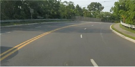
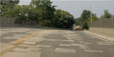
Figure 1: A highway bridge near our Holmdel office. A human designed rules-based system could navigate on the top road section, but would struggle on 50 m along the same road (bottom).

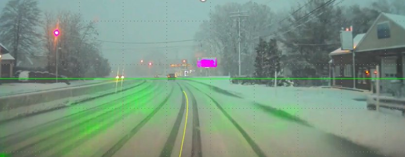
Figure 2: A snowy road in New Jersey in 2018. PilotNet was able to drive here; it would have been an extreme challenge for a handcrafted rules-based system. The green highlighted regions were most salient in determining the proper trajectory (yellow curve).

2 A Historical Perspective

PilotNet’s roots go back to 2003. At that time the Defense Advanced Research Projects Agency (DARPA) funded a six-month exploratory project to see if it was possible to learn a complete control loop from sensors to actuators. The target application was autonomous off-road navigation for mobile ground robots; the project was named “DAVE” for DARPA Autonomous Vehicle Experiment [2]. Figure 3 shows the DAVE robot.

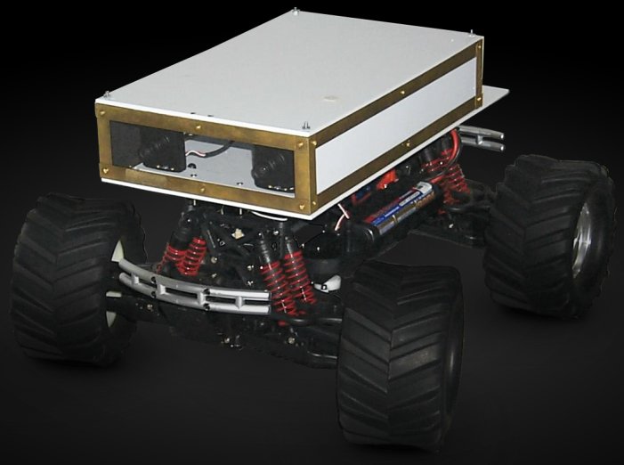
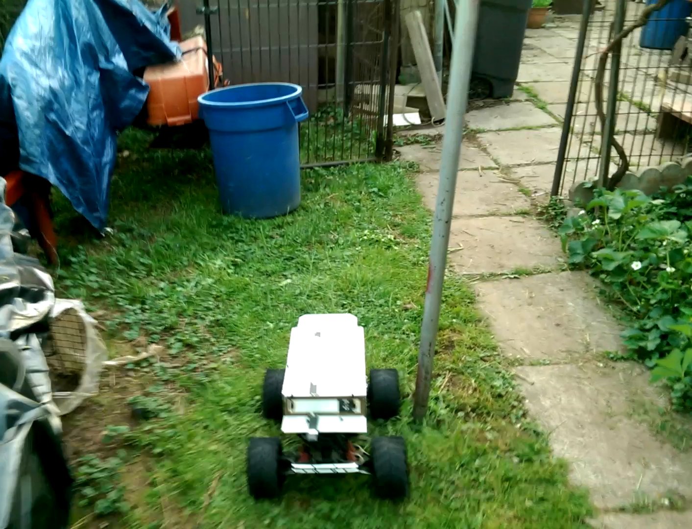
Figure 3: The robot used in the DAVE project is a modified 50-cm long model car platform controlled by a remote computer. The vehicle’s main sensors are two front cameras with 320$\times$240 pixel resolution. No explicit stereo algorithm was applied. The two camera images were simply fed to the neural network as separate planes.

DAVE learned from steering information captured while a human remote-controlled the vehicle. This end-to-end learning approach is similar to what Dean Pomerleau created at Carnegie Mellon University (CMU) in 1989 in his Autonomous Land Vehicle In a Neural Network (ALVINN) project [3]. In the intervening 14 years there were tremendous advances in computing hardware, in camera technology, and in the understanding of how to train large neural networks, so it was possible to advance beyond ALVINN. In particular, during the 1990s, the convolutional neural networks, pioneered by LeCun and his colleagues at Bell Labs [1] provided a huge performance jump in image analysis.

In the DAVE project, DARPA Program Manager Larry Jackel’s former Bell Labs and AT&T Research colleagues, Yann LeCun, Urs Muller, Beat Flepp, and Eric Cosatto demonstrated that a single convolutional neural network can be trained to drive a robot vehicle. The DAVE vehicle was a small radio-controlled robot car. DAVE was able to navigate through a home construction site littered with debris for tens of meters. While DAVE could not drive long distances without crashing, nonetheless, it held the promise of a breakthrough in autonomous driving. Images from one of DAVE’s cameras are shown in Figure 4.

In 2004 DARPA was focusing on off-road driving. To benchmark the state of the art, DARPA sponsored a Grand Challenge. Initially the plan was for competing autonomous vehicles to drive across the Mojave Desert from near Los Angeles to near Las Vegas. For logistics reasons the route was simplified to mostly follow a power line right-of-way from Barstow, California to Primm, Nevada. In this first Grand Challenge even the best participants only traveled a few miles before getting stuck. As far as we know, machine learning played little or no role in this event.

In contrast, and also in 2004, based on the success of the 6-month DAVE project, DARPA started the Learning Applied to Ground Robots (LAGR) [4] program. In LAGR, teams from top universities and research organizations competed to drive over ever more challenging courses. Teams were encouraged to use learning as much as possible in their navigation and control software. Over the 4-year lifetime of the program considerable progress was achieved.

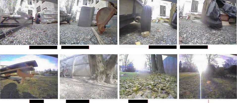
Figure 4: Snapshots from DAVE’s left camera taken while the robot drove through various environments. The black bar beneath each image indicates the steering angle produced by the system. Top row: four successive snapshots showing the robot navigating through a narrow passageway between a trailer, a backhoe, and some construction material. Bottom row, left: narrow obstacles such as table legs and poles (left), and solid obstacles such as fences (center-left) were easily detected and avoided. Highly textured objects on the ground did not detract the system from the correct response (center-right). One scenario where the vehicle frequently made wrong decisions is when the sun is in the field of view: the system seemed to systematically drive towards the sun whenever the sun is low on the horizon (right).

In 2005 DARPA ran a second Grand Challenge. This time a team led by Sebastian Thrun of Stanford won, completing the course. Part of the Stanford software stack used learning.

In 2007 DARPA ran the Urban Challenge in which autonomous vehicles competed on a course in an abandoned army base that had local streets and many buildings. In addition to avoiding other competitors, the vehicles had to contend with traffic generated by a fleet of Ford Taurus cars conservatively driven by professional drivers. Navigation in the Urban Challenge was simplified with DARPA providing dense way-points along the route and teams having access to differential Global Positioning Systems (GPSs). This was also the first event in which Velodyne LIDAR was widely deployed, giving users 3D information that proved crucial for avoiding both moving and stationary obstacles. The Urban Challenge was won by a team from CMU led by Chris Urmson.

The success of the Urban Challenge led to today’s commercial efforts to build self-driving cars. Many of the key researchers in the DARPA Challenges are leading industry efforts today and many of these efforts use ideas generated by the Challenges.

The years following the DARPA Challenges witnessed an explosion of interest in Deep Learning. Convolutional neural networks went from a shunned technology to mainstream. The realization that GPUs could vastly accelerate both the learning process and the execution (now called “inference”) of a trained neural network has played a major role in this explosion and has encouraged the idea that practical self-driving cars are possible.

In 2015 Urs Muller and Beat Flepp joined NVIDIA to help create software systems for self-driving cars. Building on the work they did for DARPA in the DAVE project they began to create a system now known as PilotNet.

3 PilotNet Overview

3.1 Evolution of PilotNet

The original PilotNet system was created by NVIDIA in Holmdel in 2015-–2016 and is described in some depth in a paper by Bojarski et al [5]. PilotNet drew on ideas developed by Pomerleau [3] (ALVINN) in 1989, and later by LeCun et al [2] (DAVE) in 2006. In both ALVINN and DAVE, recorded images of the view from the front of a vehicle were simultaneously logged along with the steering commands of a human driver creating input-target pairs. These pairs were then used for training a multi-layer neural network.

Both ALVINN and DAVE were limited by the computing resources available at the time of their creation. ALVINN featured a very small (by today’s standards) fully-connected neural network (30 hidden units) with low-resolution input images coupled with coarse range-finder input. DAVE used a convolutional neural network [1] with inputs from a pair of cameras. While DAVE’s cameras did not explicitly calculate depth from stereo, the use of two cameras meant that depth from stereo could be learned. Both DAVE and ALVINN were far from perfect, but they both represented advances over contemporaneous rule-based autonomous navigation systems.

Muller and Flepp joined NVIDIA in February of 2015 forming our core PilotNet team. We realized that creating a DAVE-like system that runs on real cars on public roads entails great technical risk and success was far from assured. Open questions included:

• Can an end-to-end approach scale to production?

• Does the training signal obtained by pairing human steering commands with video of the road ahead contain enough information to learn to steer a car autonomously?

• Can an end-to-end neural network outperform more traditional approaches?

We immediately set about to see if the DAVE concepts could be applied to on-road driving. With the addition of new hires and a pair of summer interns we began collecting driving data.

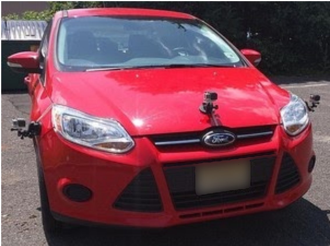
Figure 5: An early data collection car. Suction cups held GoPro cameras on the front of the vehicle, left, center, and right. The off-center cameras facilitated augmenting the training data.

In the first “hello world” experiment, GoPro cameras were mounted on the hood of a car using suction cups; one camera on the left side, one on the right, and one centered. Video was recorded from each camera as the car was driven along a road. A network was tasked to classify images as coming from either the left, center, or right camera. This task was learned successfully, giving confidence that more complex learning was possible.

In the next experiments, we utilized a stock Ford Focus, since this model’s Controller Area Network (CAN) codes for steering and speed were known to us. We could then use a consumer Bluetooth on-board diagnostics (OBD) dongle paired with a smartphone.

The cameras on our data collection car were moved to a roof rack providing better, consistent camera calibration. The CAN data was time-stamped with the phone’s network time. To synchronize the phone with the cameras, the display of a clock app on the phone was placed in front of the cameras at the start of a data collection run so that the cameras recorded the phone time. We found that the GoPros stayed synchronized with the phone time for the course of a full data collection run, typically about one hour.

In creating ALVINN, Pomerleau noted the need for augmenting the training set so that the autonomous system could drive even if the vehicle strayed beyond the range of the training data. Thus the training set was augmented with transformed images that showed what the vehicle camera might record if it had drifted away from the center of the road. These images were coupled with a steering angle that would direct the vehicle back to the center.

In PilotNet, the left and right cameras were used to provide augmented training data. These cameras recorded a view that was equivalent to that of the center camera as if the vehicle had been shifted left or right in the driving lane. In addition, all the camera images were viewpoint transformed over a range so that data was created corresponding to arbitrary shifts. These shifted images were paired with steering commands that would guide the vehicle back to the center of the lane.

The viewpoint transforms were done in the following way: first, the assumption was made that the world is flat and therefore a pixel’s vertical index corresponded to the distance of the source from the camera. The horizon was identified and all the pixels above the horizon were considered to be at infinite distance and were left untouched by the transform. The portion of the image below the horizon was skewed in proportion to the distance in image space from the horizon.

Of course, the world is not flat. Any objects above the real-world ground plane were distorted by this method. Nevertheless, the effectiveness of augmentation was proven by experiment.

It took a year from when our NVIDIA Holmdel group was formed to when we had use of a drive-by-wire car. We initially tested our ideas using a Husky [6] mobile robot. Data was first gathered using the Focus. With this data we trained a DNN to produce a steering angle given an image of the road. The trained network was then installed on an NVIDIA DRIVE™ PX system mounted on the Husky. The Husky was skid steered, so the team had to empirically translate the DNN steering command to appropriate differential wheel rotation commands to steer the Husky.

The Husky could not be driven on public roads, but fortunately near the NVIDIA office there was an off-road area with a defined path where testing was possible (Figure 6). Initial results were disappointing — the Husky would drive on the path for a few tens of meters and then drift off the path. We suspected that the network, using the perturbations, learned how to recover from shifts, but that it could not recover from rotations in which the vehicle yaw axis is misaligned with the direction of the road. To test this idea we added image transforms to the training data corresponding to rotations paired with the appropriate steering corrections. These transforms were simple, all the pixels were shifted by the same amount either left or right. The additional augmentation did the trick and the Husky could drive on the bicycle path.

In February of 2016 we took delivery of a Lincoln MKZ that was modified by the company AutonomouStuff for drive-by-wire operation and equipped with cabling for all the sensors. Also that month we moved to BellWorks, the new name for the former Bell Labs building in Holmdel where much of today’s machine learning theory and technology was created. The BellWorks complex features a garage for the MKZ as well as a few miles of private roads which are ideal for close-course testing of a self-driving car.

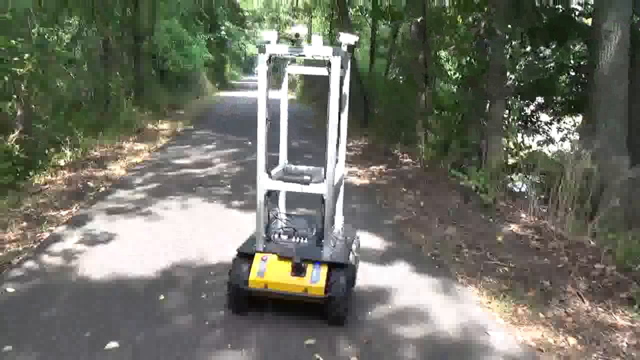
Figure 6: First field test with the Husky robot on a bicycle trail. Four cameras were mounted at about the same height where a windshield camera in a sedan would be. Only the front-facing camera was used in this experiment.

During the next month we installed cameras and the NVIDIA DRIVE™ PX board along with some support electronics on the MKZ. We created a rudimentary self-driving system by coupling PilotNet with the MKZ’s adaptive cruise control (ACC) for speed control. To our delight the car drove well on the BellWorks internal roads. (Of course, as in all our tests, we observed all relevant rules and regulations, including having a safety driver who was always on the alert to take full control of the car if needed.) The next day we took the car onto Middletown Road, adjacent to BellWorks. This is a twisty, hilly road that runs for a few miles and at the time was poorly paved. Again, the car drove credibly. The next day the self-driving MKZ (with a few interventions) took team members to a nearby restaurant to celebrate. The system was first shown to the public at the GPU Technology Conference (GTC) San Jose in the Spring of 2016 (available on Youtube) and later at GTC Europe in the Fall of 2016 (available on Youtube).

Over the next nine months the self-steering system, now known as PilotNet, was rapidly improved, culminating in a public demonstration on a closed course at the 2017 Consumer Electronics Show (CES) in Las Vegas.

The CES demo was set up just before Christmas in an unusual rainy spell in Las Vegas. The car was tuned to drive well in the demo by using training data recorded on the demo course which included a variety of road surfaces (paved, gravel, grass) and some movable construction obstacles. When the weather cleared and the sun came out, the car’s performance declined. Also, as the start of CES approached, the fencing and banners around the test course were changed and the car failed to stay in the lanes. Rapid on-site retraining of PilotNet with additional data that included different lighting and different objects at the track perimeter fixed the problems and the car drove well throughout the event. During CES, hundreds of passengers rode in the back seats of the PilotNet driven MKZ and an SUV provided by Audi. The 2017 CES demo course is shown in Figure 7 and reported by various on-line publications, for example by The Verge.

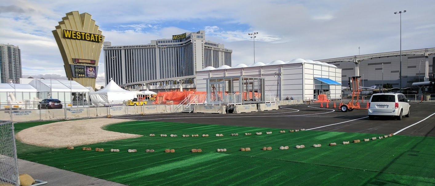
Figure 7: The CES 2017 demo course before the show opened.

We defined a metric for benchmarking PilotNet performance: mean distance between failures (MDBF) which is the average distance traveled between required human interventions. Early versions of PilotNet were trained on a few hours of human driving data on both highways and local roads. Early PilotNet had an MDBF of about 10 km: it was able to steer an average of about 10 km in the center lane of the Garden State Parkway near Holmdel, NJ. Here, there are three lanes in each direction of the limited access highway. PilotNet was also able to steer on local roads, but a human operator had to intervene at intersections since early PilotNet had no route planning capability and could not initiate turns.

3.2 Learning a Trajectory

Early PilotNet produced a steering angle as output. While having the virtue of simplicity, this approach has some drawbacks. First, the steering angle does not uniquely determine the path followed by a real car. The actual path depends on factors such as the car dynamics, the car geometry, the road surface conditions, and the transverse slope of the road (banks or domes). Ignoring these factors can prevent the vehicle from staying centered in its lane. In addition, just producing the current steering angle does not provide information about the likely course (intent) of the vehicle. Finally, a system that just produces steering is hard to integrate with an obstacle detection system.

To overcome these limitations, PilotNet now outputs a desired trajectory in a 3D coordinate frame relative to the car coordinate system. An independent controller then guides the vehicle along the trajectory. Following the trajectory, rather than just following a steering angle, allows PilotNet to have consistent behavior regardless of vehicle characteristics.

An added bonus in using a trajectory as an output is that it facilitates fusing the output of PilotNet with information from other sources such as maps or separate obstacle detection systems.

To train this newer PilotNet, it is necessary to create the desired target trajectory. Initially, we used the trajectory followed by a human driver in the data collection car as the target trajectory. This trajectory was extracted from the vehicle pose derived from recorded vehicle speed, inertial measurement unit (IMU), and GPS sensor data. We later discovered that the human-driven trajectory, coupled with data augmentation, resulted in poor on-the-road driving (see Section 9). We now use the lane centerline, as determined by human labelers, as the ground-truth desired trajectory. See Section 5.1.

3.3 Additional PilotNet Outputs

PilotNet now provides multiple outputs that correspond to seven possible trajectories. An external navigation system chooses among these trajectories to guide the vehicle. The possible trajectories are:

• Lane stable (keep driving in the same lane)

• Change to left lane (first half of maneuver)

• Change to left lane (second half of maneuver)

• Change to right lane (first half of maneuver)

• Change to right lane (second half of maneuver)

• Split right (e. g. take an exit ramp)

• Split left (e. g. left branch of a fork in the road)

In addition, PilotNet now predicts lane boundaries that are inferred even when there are no lines painted on the road. The lane boundary output allows third parties to plan their own trajectories using the path perception provided by PilotNet.

4 Data Collection and Curation

Creating a huge, varied corpus of clean, accessible data is one of the most critical and resource-intensive aspects encountered in creating a high-performance, learned self-driving system. In this section we describe our data collection and curation process.

4.1 Early Data Collection

To see if our ideas held promise, we did some rapid prototyping. As previously mentioned, we trained early versions of PilotNet using video from GoPro cameras mounted with suction cups on our data collection cars. See Figure 5. The cars were driven primarily within Monmouth County, New Jersey under various weather and lighting conditions. Data was recorded using an NVIDIA DRIVE™ PX system.

4.2 Hyperion Data

The early data was adequate for demonstrating a proof-of-concept, but to get to a high-performance product, a massively scaled data collection process was required. Recognizing this need, in 2017 NVIDIA embarked on a large-scale data collection campaign. This effort, known as Hyperion [7], included building a fleet of Ford Fusion and Ford Mondeo cars to collect data not only for PilotNet but also for numerous other subsystems required for a complete driving solution.

Collected data included imagery from 12 automotive-grade cameras, returns from 3 lidars and 8 radars, GPS data, as well as CAN data such as steering angle and speed. Computing for the data collection platform was provided by two NVIDIA DRIVE™ PX 2 systems. Data was collected in the U.S., Japan, and Europe with routes chosen to maximize diversity. Figure 8 shows one of the Hyperion data collection cars.

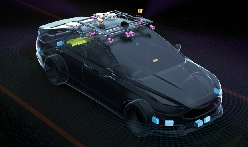
Figure 8: NVIDIA Hyperion data collection vehicle sensor layout [7].

5 The Training Pipeline

Training PilotNet is a complex, multi-stage process that requires manipulating huge quantities of data as well as extensive computing. To train PilotNet efficiently we developed a comprehensive automated data pipeline. The pipeline lets us simultaneously explore different adjustments to network architecture, data selection, and image processing. In addition, the pipeline allows us to run experiments reproducibly; much effort was expended to ensure deterministic behavior. Elements of the pipeline are described below.

5.1 The Labeling Process

Collected data was processed using the PilotNet labeling tool in which human labelers can quickly examine recorded video and segment it into clips representing different driving maneuvers (lane stable, lane change, lane split, merge, turn). In addition, the data is tagged for different conditions such as road type (multi-lane highway, single-lane highway, unmarked road), road condition (dry, wet) and for special events such as avoiding an obstacle. See Figure 9.

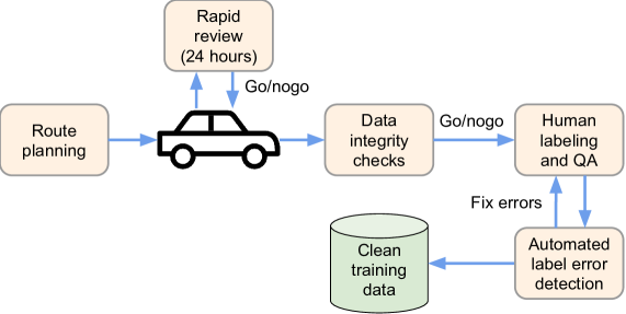
Figure 9: Diagram outlining Hyperion data collection, rapid field review, labeling, QA, and data archiving. The process strives to produce and store only high-quality data. Rapid field review ensures that we can react to basic data quality problems quickly (e. g., if sensors are not recording). The data integrity checks run in the cloud and analyze the data quality in detail (e. g., proper time stamps). However, it can take several weeks before the data becomes available in the cloud.

The labels go through a QA process, where multiple labelers check each other’s work. The best labelers become quality assurance staff, checking on the work of the other labelers. In addition, we run a trained PilotNet network over the new labeled data and flag instances where the network trajectory output has a large discrepancy compared to the label. These segments are then checked by the most experienced labelers to make sure the labels are correct. Bad segments are then re-labeled. We refer to this process as “bad appling,” since we discovered that a few mislabeled critical segments can create unexpected failure modes in the system.

As data is cleaned, labeled, and archived, small chunks of this new data are added to our active training data set and a preliminary new PilotNet is trained. Test results are compared with the previous version of PilotNet to make sure that that additional data improves overall performance. If performance degrades, the new data undergoes further scrutiny to uncover the reason for the degradation.

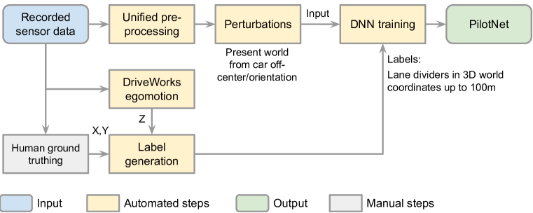
Figure 10: A data-flow diagram showing how labels are generated for training a PilotNet network. The input on the top left and the manual steps on the bottom left correspond to processes outlined in Figure 9.

PilotNet employs a supervised learning framework to train a neural network to predict trajectories that the vehicle should follow. To train such a network, labelers mark the edges of the lanes driven by professional human drivers. The points along the center line between these edges are defined as the desired $X$ and $Y$ trajectories and become the ground truth $X$ and $Y$ labels. The training trajectory’s vertical ($Z$) component is calculated using the vehicle egomotion, i. e., the relative position and orientation of the vehicle as a function of time. The egomotion module, which was created by the NVIDIA DriveWorks [8] team, uses IMU, odometry, and GPS recordings with a vehicle motion model to deduce the egomotion of the vehicle in 3D. The data-flow diagram for training PilotNet is shown in Figure 10.

During inference time, PilotNet provides desired trajectories in the vehicle’s local coordinate frame. In a preprocessing step, PilotNet’s trajectory generation module first creates the trajectory of the entire recording in a global coordinate frame. Then a library of trajectory transformation algorithms extracts segments of this trajectory data that corresponds to each training frame. The library also transforms the trajectory segment from the global world coordinate frame to the vehicle’s local coordinate frame that is used during training.

5.1.1 Training Label Generation

Human labelers annotate driving maneuvers (lane stable, lane change, lane split, merge, turn), road types (multi-lane highway, single-lane highway, unmarked road), road conditions (dry, wet) and special events such as obstacle evasion and speed changes to comply with traffic rules (i. e., stopping at a traffic light). Some of these annotations are used for generating control inputs sent to the network at training time. The rest are used for filtering and sampling the data.

The trajectory label, derived as described in Section 3.2, consists of 100 3D points spaced one meter apart. These points are referenced relative to the car coordinate system.

5.2 Preprocessing

Camera image characteristics vary depending on camera type and on camera location and orientation. Preprocessing reformats image training data, compensating for these variations. The remainder of this section describes this preprocessing pipeline.

5.2.1 Image Pinhole Rectification

First, camera images are reformatted so that they appear as if they were recorded by an ideal (pinhole) camera. This step removes distortions that are particular to the camera lens, rendering the image lens-independent. Thus PilotNet can be made robust to variations in intrinsic camera parameters. This means the network can be trained on images gathered from one set of cameras and later produce driving trajectories for images created by a different set of cameras.

5.2.2 Viewpoint Transformation

Second, camera images are transformed so that they appear to be captured from a standard position and orientation on the vehicle. All points in the training trajectory are measured relative to the rear axle of the vehicle, so the transformed images appear as if the camera is 1.47 m above the rear axle and 1.77 m in front of the rear axle along the center line of the car. These numbers come from the actual camera placement on most of our data collection cars. However, we want PilotNet to work on other cars in which the camera may be in a different location. With this “viewpoint” transformation the processed images become nearly independent of the precise camera placement on the vehicle.

We note that the viewpoint transformation cannot be perfect, since there are bits of the road ahead that may be visible from one camera location and not visible from another. However, these discrepancies are small when we consider portions of the road that are beyond a few meters in front of the vehicle.

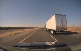
(a) Original camera image

(b) Pinhole-transformed image

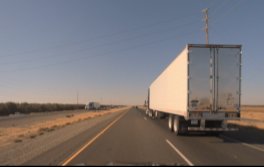
(c) Viewpoint-transformed to standard camera position

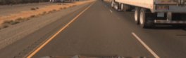
(d) ROI cropped image

Figure 11: Examples of rectifying and transforming an image to a standard format and resulting ROI.

Third, images are cropped to a ROI. The boundaries of this ROI are in 3D world coordinates rather than image space. The specifics of the ROI are chosen in the following way: first we set the horizontal field of view to be 53^∘ wide. Next we assume the ground is flat and we choose the top of the ROI to align with to the horizon. Finally we adjust the bottom of the ROI to correspond to a section of the ground that is 7.6 mwide. With these adjustments in mind, the images are linearly scaled so that the resulting image is 209 pixels wide and 65 pixels high. Refer to Figure 11.

By choosing these parameters we eliminate the sky which has little bearing on driving. Provided the camera has sufficient resolution, we create standardized images that are largely independent of camera properties.

5.3 Training Data Augmentation

We observed in early experiments that, when PilotNet’s neural network was trained only with samples where the vehicle is aligned with the target trajectory, the network had challenges predicting the correct trajectory if the vehicle deviated from the center of the road. This occurred because off-road-center driving is outside of the original training data. As a result, the driving system could not recover from a series of network errors, controller errors, or environmental factors that would cause the vehicle to deviate from the lane center. This is a well known problem with imitation learning [3, 9, 10].

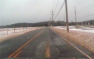
(a) Original image

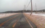
(b) 1 m shift right

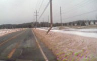
(c) 1 m shift right, 10^∘ rotate right

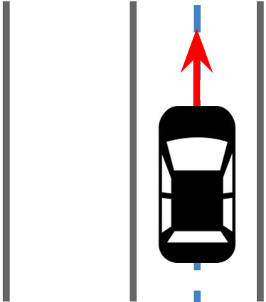
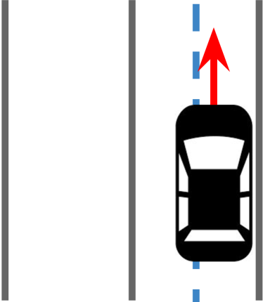
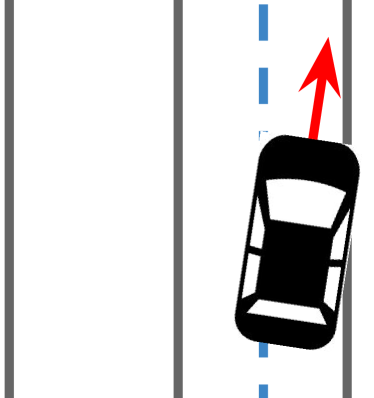
Figure 12: Illustration of transforming camera data with a flat-world assumption to emulate a shift and rotation of the vehicle.

To mitigate this issue, we augment our data with training images that make the vehicle appear shifted from the lane center and/or rotated from the lane direction. We use the same viewpoint transforms we use to transform camera images to a nominal position to emulate a shift and rotation of the camera. Figure 12 illustrates the viewpoint transformations used to augment training data.

There is one caveat of using viewpoint transforms for virtually moving a camera: we do not have accurate 3D geometric information about the world, so we assume a flat world and transform the image according to that geometry. This creates distortion artifacts on any object in the image that does not fit our flat-world assumption. See Figure 13.

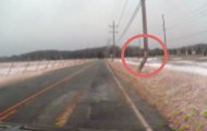
Figure 13: Resulting artifacts that occur because of an incorrect flat-world assumption. Vertical features whose base is below the horizon in the image are distorted. As an example, look at the utility pole marked by the red circle.

Because these artifacts carry information about the shift and rotation of the augmentation, it is possible that these artifacts could become a dominant signal that the network uses to learn the training labels rather than using the image of the road. A more detailed discussion of this effect is presented in Section 9. To lessen this possibility, we record from multiple (typically three) cameras placed at different shifts on the vehicle and stochastically select which of these cameras to use in a training example. Because the cameras each have a different original position, the resulting distortion artifacts are different depending on which camera we are using for the training example. This procedure introduces variation to the distortion signal to discourage the network from learning a correlation between the distortion artifacts and the off-center position of the vehicle. In addition, human driving behavior during data collection frequently deviates from the center of the lane (standard deviation typically is 20 cm). This adds additional shift and rotation variations relative to the true center trajectory we use as the training label today.

6 PilotNet Neural Network Architecture

Early PilotNet followed a typical convolutional neural network structure [1]. More recent versions feature a modified ResNet structure [11]. See Figures 14-–18.

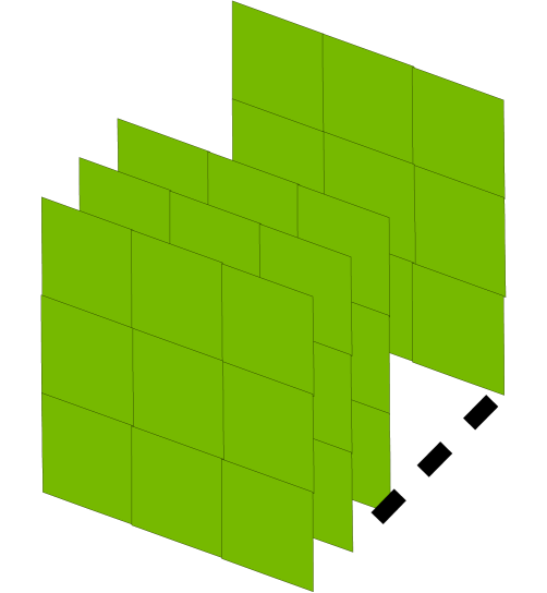
(a) 2D convolution

(b) ReLU

(c) 2D Batch Norm

(d) Linear Addition

(e) Spatial Dropout

Figure 14: The five basic building blocks of PilotNet shown in Figure 15

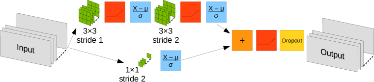
Figure 15: A basic residual block. All 3$\times$3 kernels use padding of 1. Padding adds $N$ pixels at the edges of the input matrix, which is necessary for the convolution operator to be properly applied to the cells at the edges.

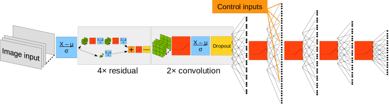
Figure 16: The full PilotNet training architecture. Sizes of the intermediate steps appear in Table 1. Control inputs to control network driving behavior (split, lane change, etc.) are added to the inputs of the second fully connected layer.

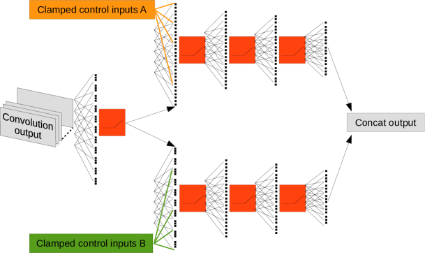
Figure 17: The exported version of the PilotNet network with modifications for simultaneous trajectory outputs without requiring control input selection. The fully connected layers are cloned and the control inputs are frozen for each output. This can be done with any number of behaviors, only two are visualized here. For run-time optimization it is also possible to convert the cloned linear layers into sparse convolutions.

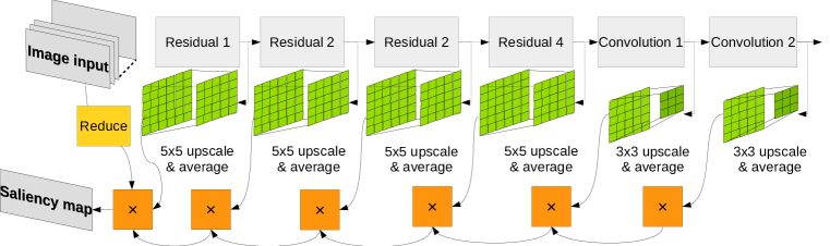
Figure 18: Outputs of the residual and convolution layers are upscaled, averaged, and multiplied to create a single-channel saliency map (i. e., finding the pixels that are most crucial in determining the driving trajectory [12].

Layer name	Output size
Batch norm 1	3$\times$113$\times$209
Residual 1	48$\times$57$\times$105
Residual 2	72$\times$30$\times$53
Residual 3	96$\times$15$\times$27
Residual 4	128$\times$8$\times$14
Convolution 1	192$\times$6$\times$12
Convolution 2	256$\times$4$\times$10
Flatten	10,240
Linear 1	256
Linear 2	256
Linear 3	128
Linear 4	96
Linear 5	Target

Table 1: Output sizes of PilotNet layers. The exact number of outputs is determined by the training target (number of paths, number of dimensions, etc.).

6.1 Control Inputs

To proceed beyond simple lane following, an autonomous car must be able to switch lanes, negotiate lane merges and splits, and execute turns. PilotNet has been extended to support these tasks. As shown in Figure 16, we can accommodate an arbitrary number of behaviors by creating a control input vector for each behavior and feeding it into a clone of the last four linear layers. A control system receives all the outputs of the network and decides which to use based on the current maneuver. For runtime execution (inference), the trained network is exported using NVIDIA TensorRT, which generates optimized CUDA kernel schedules to increase inference performance on the NVIDIA DRIVE™ AGX in the vehicle.

6.2 Large-Scale Training

PilotNet currently trains on millions of frames. All data manipulation is executed in parallel on one of NVIDIA’s internal GPU compute clusters. Training a PilotNet network from scratch to peak driving performance takes about two weeks.

Instead of augmenting our training data online, we augment the samples prior to the training step. By processing the data once, saving it to disk, and reusing it in each epoch we save considerable compute time. Training samples are shuffled during the off-line augmentation process so that data can be read sequentially during training.

The training samples are considerably smaller in size compared to the full-resolution video frames; therefore loading the preprocessed samples from disk by itself, reduces the compute and I/O bandwidth required per epoch. In addition, the augmented data can be re-used across multiple experiments (such as neural architecture search, hyperparameter tuning, or simply training with multiple seeds for the random number generators), further reducing the compute requirements of developing PilotNet.

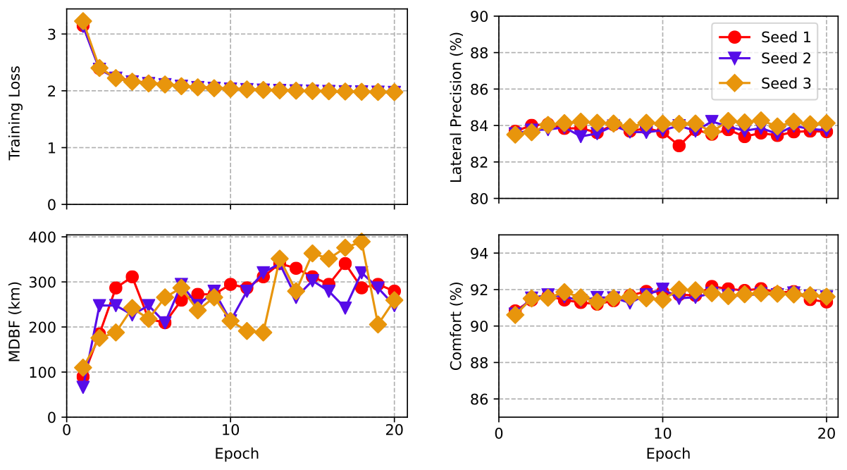
Figure 19: Evolution of training loss and driving performance during training, measured for three different neural networks initialized with different seeds. See Section 6 for the definition of the performance metrics.

Processed and augmented frames, as well as the labels for these frames, are stored as flat serialized binary files for fast data I/O. We developed a custom data storage library in order to write and access these files. The library is implemented in C++, and has Python bindings for easy integration with the PyTorch data loader.

After each epoch of training, we launch a parallel task to measure the performance of the network in augmented resimulation (see Section 6.3 below). This way, we not only monitor the training loss, but also the metrics that are more relevant to the task, i. e., the real-world driving performance. Figure 19 shows the per-epoch training loss and driving performance for three networks initialized with different seeds.

6.3 Testing the Network: The Augmented Resimulator

We require a means to evaluate and compare different versions of PilotNet. The most direct test is real-world on-road testing. However, real-world tests are time consuming, not easily reproduced, and have risk. Simulated test environments can help alleviate some of these issues, but simulations may not be representative of the real world. This is a particular concern for vision-based systems like PilotNet, where road textures, glare, or even chromatic aberration caused by different speeds of capturing the red green blue (RGB) channels in the camera can affect real-world driving. Producing a photo-realistic simulation can be a challenge in itself.

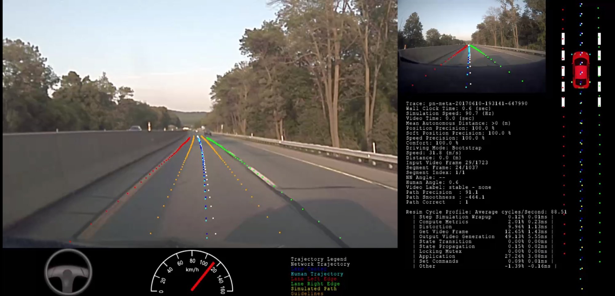
Figure 20: Screenshot of the Augmented Resimulator. The car icon in the upper right corner shows the position of the resimulated vehicle in its lane. The photographic image in the upper right is the original image captured while the data collection car was driven by a human. The large image on the left is the resimulated view. The dashed dark blue line indicates the ground truth lane center. The dashed light blue line represents the path driven by the human driver. The white dashes is the predicted path from the neural network. The yellow dashes are the tire positions from the resimulation. The red and green lines are the predicted lane edges.

In response to the challenges of creating realistic simulations, we created the Augmented Resimulator tool, a solution that allows for closed loop testing like in a synthetic simulator but working off real sensor recordings instead of synthetic data. As mentioned in the preprocessing section, PilotNet utilizes viewpoint transforms to expand the training data to domains not recorded through human driving (Section 5.2.2). We leverage the same strategy to generate testing environments from collected videos. Figure 20 shows a screenshot of the Augmented Resimulator.

The basic approach is similar to video-replay, except the system under test is free to control the car as if it was in a synthetic simulation. At each new state of simulation, we produce sensor data for the cameras through a viewpoint transform from the closest frame in the recording. As long as the system under test doesn’t deviate too much from the recorded path, we will always have sensor data available. If the network deviates too much from the recorded path, then we will not have sufficient sensor information available to apply our transformations; therefore in these instances we reset the simulated vehicle to the center of the road. Of course, if we deviate too far, we also consider this to be a failure. With this tool, we use data collected from real-world cameras so that we do not have to re-create the world photo-realistically in simulation.

Our approach is not without limitations, namely, the presence of image artifacts as mentioned in Section 5.2.2. Furthermore, our driving scenarios are limited to data we recorded. We cannot, for example, change the time of day on the fly as is possible in synthetic simulation, nor can we take any turns or highway exits unless they were recorded. We do, however, gain the advantage of having as much simulated data as we can collect and label without the need to design simulated cities and roads. Furthermore we can accurately reproduce the exact scenario of real-world failures.

6.4 Detecting Failures

One metric that we are particularly interested in is the MDBF (see Section 7 for more information). We define MDBF as the distance driven under test, divided by the number of failures in that distance. A naive criterion for failure is to detect if there is a large lateral deviation from the human-driven trajectory. However, this approach can fail when the road becomes too wide, or if the human-driven path is not in the center of the road. To better facilitate failure detection, we add additional labels per frame in our test set recordings. These labels indicate the locations of the left and right lane boundaries. If any of the wheels of the simulated car touches these lane boundaries, we flag this as a failure.

6.5 In-Car Monitor

We have created an in-car monitor to aid in system development. The monitor, showing PilotNet’s inputs and outputs, gives humans a real-time view of PilotNet’s performance. See Figure 21. A key feature of the monitor is the several trajectories predicted by PilotNet for different maneuvers. In the image, these trajectories are 100 m long.

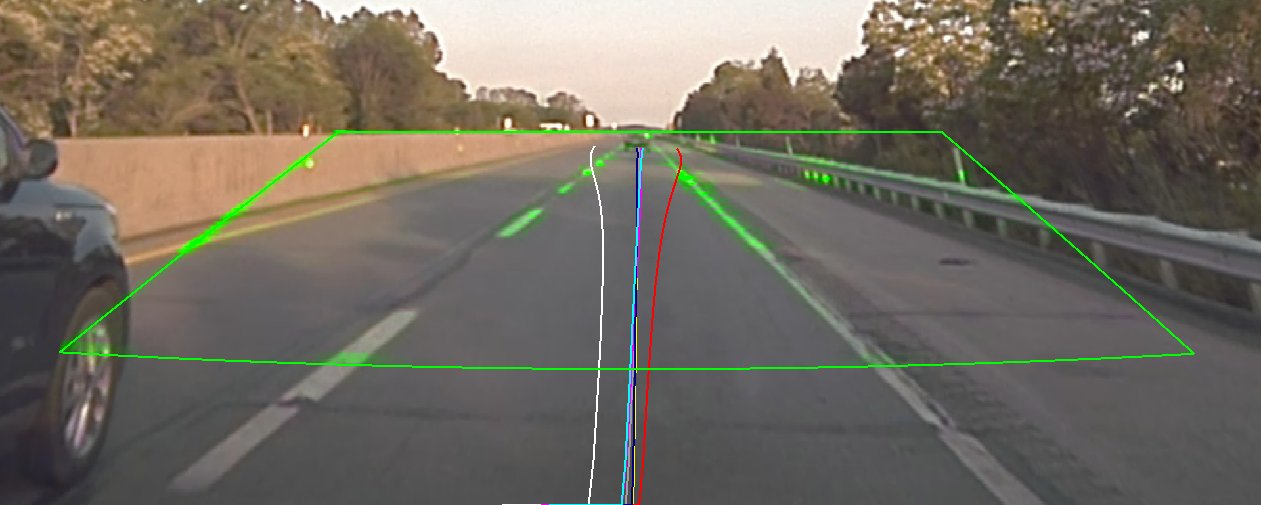
Figure 21: PilotNet in-car monitor showing the ROI (green trapezoid) and the seven predicted trajectories. The reason the trapezoid edges appear curved is that inference occurs on rectified images while the car display shows the original unrectified camera image. The straight line of the trapezoid in the rectified image therefore become slightly curved in the display image.

6.6 Where Does the Network Look?

The in-car monitor includes a saliency map that highlights (in bright green) the regions of the input image that are most salient in determining PilotNet’s output. The methodology in creating this visualization is described in Bojarski et al [12]. Figure 18 demonstrates how the saliency map is computed. Figure 22 shows some examples of saliency maps.

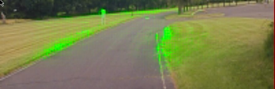
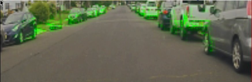
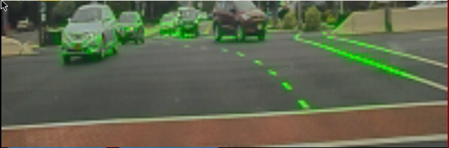
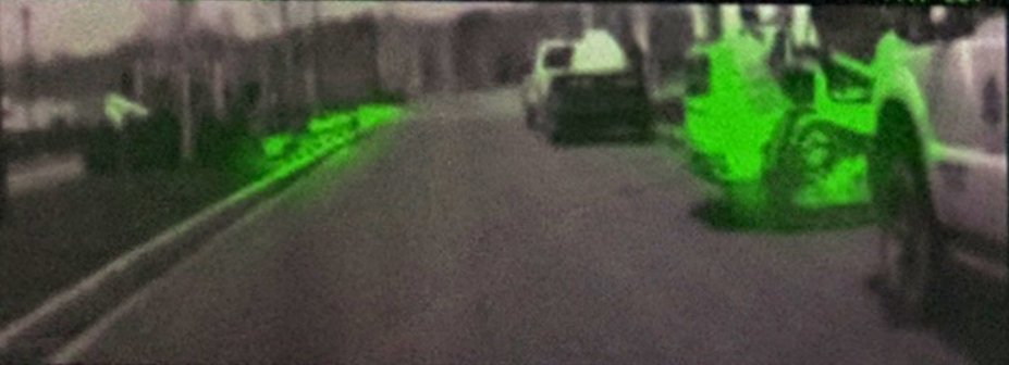
Figure 22: PilotNet saliency maps. The top image shows a narrow road with no lane markers. The network focuses on the grass-pavement boundary. The next lower image shows a residential street with no lane markings. Here the lower parts of the parked cars guide PilotNet. The third image from the top shows a busy intersection. Pilot pays attention to painted lines in the direction of travel, but ignores lines of the crosswalk that are nearly perpendicular to the direction of travel. In the bottom image PilotNet is guided by the BobCat front loader on the right and the curb on the left.

7 Metrics and Performance History

A number of metrics are used to evaluate PilotNet performance. Most critical is MDBF. MDBF measures the average distance PilotNet can steer an autonomous vehicle before a human must take control to avoid a dangerous situation. MDBF is evaluated in specific domains. Currently we are focusing on highway driving, which means stretches of divided, limited-access roads, such as US interstate highways. We exclude places where the highways split or merge and where navigation instructions are more complex than just “follow the road.” In on-the-road tests, PilotNet was able to steer from Holmdel, New Jersey to North Carolina and back with only one highway intervention over a distance of about 1,300 km. (video NC to NJ). We note that the conditions on this trip were not ideal, with stretches of heavy rain and nighttime driving. Figure 23 shows the evolution of MDBF.

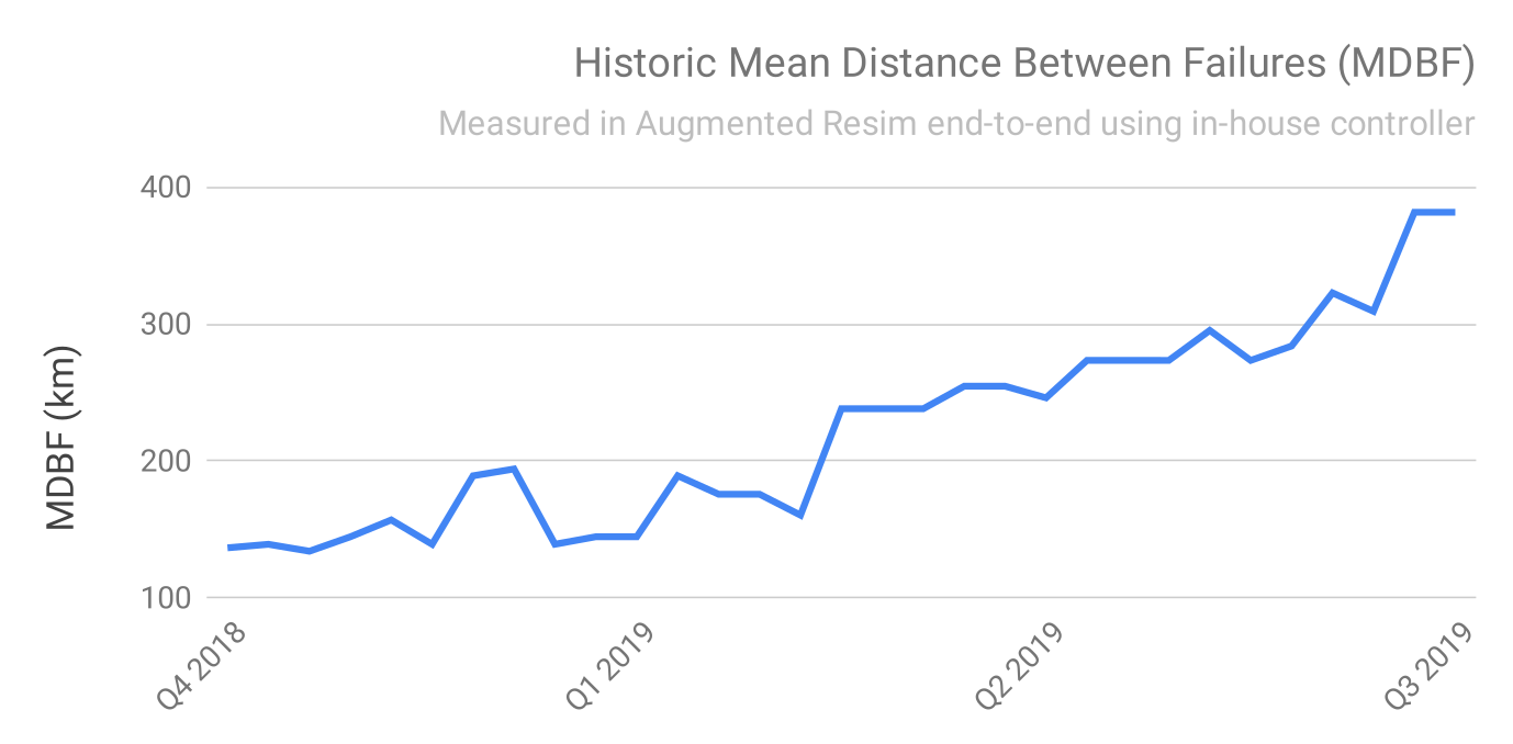
Figure 23: Evolution of PilotNet’s MDBF over time. Note that the MDBF reflects the combination of the neural network and controller performance. Both are improved independently which can lead to temporary regressions of the overall driving performance. For example, as the controller was improved to more faithfully follow the predicted trajectory, shortcomings of PilotNet’s predictions were uncovered.

Another metric is “precision” or how closely the vehicle tracks to the lane center. Our definition of precision is 100$\times$(1 m - RMS deviation from lane center in meters) / 1 m. Right now we can only measure precision for PilotNet in simulation (see section 6.3). Typical values are 80%. We find that for human drivers precision is typically 66%.

The final metric we track is “comfort,” which is a measure of the “smoothness” of the ride as measured by sensors on the vehicle. As we measure it, comfort is determined by the root mean square (RMS) of the time derivative of the vehicle’s lateral acceleration. The comfort scale is somewhat arbitrary, but we set constant acceleration to correspond to a comfort of 100 and have comfort decrease in proportion to the RMS time derivative of the vehicle acceleration. Human-driven vehicles typically have comfort scores around 80. We achieve similar scores in simulation with the current version of PilotNet. We hope to measure PilotNet on-the-road comfort soon. One limitation of this metric is that the comfort score drops when the vehicle enters a curve (due to the increased lateral acceleration), even though the vehicle may be driving perfectly in the center of the lane.

8 Multi-Resolution Image Patches

8.1 Introduction

Learning an accurate trajectory requires high-resolution data that provides enough information for PilotNet to see clearly at a distance. High-resolution cameras are used for this purpose. However, the image preprocessing steps, such as cropping, and downsampling significantly reduce resolution. In the early versions, the preprocessed image patch fed into PilotNet had a size of 209x65 pixels. One of the advantages of a small patch size is that it reduces the computing load, allowing PilotNet to drive with a high frame rate. But the resolution (about 3.9 pixels per horizontal degree and about 5.9 pixels per vertical degree) at large distances is too low for the network to extract needed road features. To illustrate, at this resolution, the full moon would be only 2 pixels wide.

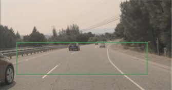
(a) Original image

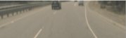
(b) Regular patch

Figure 24: The original pinhole image is shown in 24(a) with the green rectangle indicating the ROI. The image in  24(b) shows the downsampled 209$\times$65 image. Note how few pixels are dedicated to the off ramp.

Figure 24(a) shows an example of an original image from the camera and Figure 24(b) shows the processed image patch. Note that in the patch, the off-ramp in the road ahead is barely visible. This low resolution can confuse PilotNet, with the predicted path swerving right before the off-ramp. One of the solutions to this problem is to increase the patch resolution at large distances. The most straightforward method is to uniformly increase the patch resolution by reducing downsampling. However, uniformly increasing the patch resolution will quadratically increase the computational burden. For example, increasing the resolution five times from 209$\times$65 to 1045$\times$325 requires 25 times more computation in neural network training and inference.

To increase the resolution at far distances while keeping a near constant computational load, we introduce a new method we call “multi-resolution image patch.” This method significantly improves the PilotNet performance with modestly more computation, allowing PilotNet to increase its MDBF by about 50%

8.2 Creating the Image Patch

The basic idea of the multi-resolution patch is to linearly increase the horizontal and vertical resolutions (pixels per degree) from near to far distance with respect to the regular image patch. The method we used here extracts a trapezoidal ROI from the original image and then reshapes it into a rectangular patch. Figure 25 shows how the multi-resolution patch is generated. Each pixel in the image patch corresponds to a source area in the original image, and the pixel value is the average value of the source area.

Figure 25: The ROI for the multi-resolution patch is a trapezoid. It is downsampled to generate a multi-resolution patch as shown on the bottom right.

Let’s denote the top width, the bottom width and the height of the ROI in the original image as $roiTW$, $roiBW$ and $roiH$, and the width and height of the image patch as $patchW$ and $patchH$. The bottom width and height of the source area are denoted as $dW$ and $dH$. For the multi-resolution patch, in pixel space, the width and height of the source area are linearly increasing from top to bottom. Here, we use a horizontal resolution ratio ($ratioW$) and a vertical resolution ratio ($ratioH$) to define the source areas. The horizontal/vertical resolution ratio is defined as the width/height ratio of the bottom source area to the top source area. The mathematical definition is as follows.

$$dW(i) =a_{w}{}*i+b_{w}, i=0,1,\cdots,patchW -1$$ (1)

$$dH(i) =a_{h}{}*i+b_{h}, i=0,1,\cdots,patchH -1$$ (2)

With constraints:

$$dW(patchH-1) =roiBW/patchW$$ (3)

$$ratioW =dW(patchH-1)/dW(0)$$ (4)

$$ratioH =dH(patchH-1)/dH(0)$$ (5)

$$\sum_{i=0}^{patchH-1}dH(i) =roiH$$ (6)

where $i$ represents a row index starting at $0$ for the topmost row of source areas. Hence, given $roiBW$, $roiH$, $patchW$, $patchH$, $ratioW$ and $ratioH$, we can calculate the size of all source areas using the above equations.

After defining the multi-resolution source areas, we downsample each source area to one pixel by averaging the original pixel values, obtaining the multi-resolution patch. Note that setting $ratioW=1$ and $ratioH=1$, the generated patch is the same as the original patch.

8.3 Experimental Results

To evaluate the performance of the multi-resolution patch, we performed a parameter search on $ratioW$ and $ratioH$ with fixed $roiBW$, $roiH$, $patchW$, $patchH$ and $dH(patchH-1)$. Holding $dH(patchH-1)$ constant ensures that the resolution at the bottom of the resampled image remains fixed.

The dataset for the parameter search contained 20 hours of training data and 14 hours of testing data. The optimal parameters reported by the parameter search were further validated using a larger dataset (260 hours of training data and 80 hours of testing data). The optimal settings for PilotNet is $ratioW=2$ and $ratioH=8$ with a patch size of 209$\times$113. That is, the horizontal and vertical resolution of the top pixels of the multi-resolution patch are 2$\times$ and 8$\times$ larger than those of the regular patch, respectively, which only increases the computational load by 70%.

The multi-resolution network (i. e., the network trained with the multi-resolution patch) achieves a significantly higher performance in the Augmented Resimulator (Section 6.3) both in terms of MDBF (increased by 50%), comfort (increased by 3%), and precision (increased by 2%). Multi-resolution also helps PilotNet avoid swerving at off-ramps and other scenarios where lanes split. Figure 26 shows some example patches where the multi-resolution network predicts a better driving trajectory than the regular network.

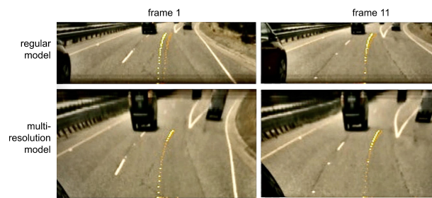
Figure 26: The yellow lines are ground truth trajectories, and the orange lines are the network-predicted trajectories. The multi-resolution PilotNet neural network achieves higher prediction accuracy. These are two example frames near forks.

We also tested the multi-resolution network in the car and compared it with the regular network. Results were consistent with resimulation results; the multi-resolution network drove smoothly at splits without swerving (unlike the fixed-resolution network).

Multi-resolution image patches are now used in PilotNet by default. This method increases the resolution of far-distance pixels with slightly more computation in network training and inference. The method is much less computationally expensive than simply increasing the patch resolution with the same aspect ratio.

Note that the multi-resolution patch is “distorted” with respect to the regular patch. However, this distortion is not a problem for PilotNet since the network is able to learn the relationship between the multi-resolution image space and 3D world space.

9 Tuning the System

9.1 A Detective Story: Catching a Network that Cheats

As new versions of PilotNet were produced, performance in the Augmented Resimulator tracked real on-the-road performance so that Resimulator performance was assumed to be a reliable indicator of what we would see in a real car.

In mid 2019 with increased training data, with tweaks to the network architecture, and with adjustments in data sampling, MDBF as measured in the Resimulator continued to increase, but to our shock, performance on the road became less stable. What was going on?

We got a hint that something was amiss when we saw in resimulation that networks trained to only stay in lane did perfect lane changes. In these instances, video sequences that captured lane changes were accidentally included in the resimulation tests. After much thought we realized that the network was inadvertently trained to generate paths that minimize perturbation artifacts of the training images. Somehow the network was keying on artifacts generated by the perturbations. In effect, the network was getting high marks in resimulation by ”cheating”: it was using resimulation artifacts to define the vehicle path rather than actual features of the road. We realized that our efforts were essentially human-engineered gradient descent in network hyperparameters space seeking to maximize resimulation MDBF.

Where do the artifacts come from? Recall that the Augmented Resimulator produces simulated sensor images that are derived from real-world recordings. Since the simulated vehicle may drive a different path than the vehicle in the real-world recording, the real-world and simulated sensor positions will differ. Therefore, a transformation must be applied to the real-world sensor data in order to “simulate” the alternate state that would be observed by the sensors in the Augmented Resimulator. For example, if the simulated vehicle tracks towards the right with respect to the real-world car, the camera sensor generated image should show the view from the simulated car as if it is driving closer to the edge of the right lane. As we discussed in Section 5.3, our transformations make a flat-world assumption; any real objects that stick up above the ground plane will have distortion artifacts. As examples, look again at Figures 12 and 13.

We found it is possible that a network trained with the same perturbation transformations as used in the Resimulator will utilize the perturbations to gain an artificial improvement in Resimulator metrics (i. e. the network learns to cheat). This effect has been named model affinity to perturbation artifacts (MAPA). A network that is affected by MAPA has a tendency to follow the real-world human driving in resimulation, scoring good metrics. Even though the network may have good scores in Augmented Resimulation, it will drive poorly in the real world, where these augmentation artifacts are not present. We note that cheating is even observed on synthetic flat-world images. It appears that networks can learn to cheat not only on clearly distorted images like lampposts, but even on subtle pixel-level effects not visible to humans.

9.2 Measuring if the Network is Affected by Augmentation Artifacts

In order to examine whether a network is using augmentation artifacts to gain an artificially inflated score in the Augmented Resimulator, a specific test was created. Data was collected on the New Jersey Garden State Parkway (NJ-GSP) by driving the route twice, first with the human driving close to the left edge of the lane, and later, with the human driving close to the right edge of the same lane. Two separate Resimulations were executed, one using the left-biased recording, and the other using the right-biased recording.

If the network is not affected by MAPA, it is expected that the network will drive in the center of the lane in both Resimulations. If the network is affected by MAPA, it is expected that it will be biased in the same direction as the human.

9.2.1 MAPA Score

We created a formula using the mean values of bias in this test to compute a MAPA score. We wanted this score to have the following properties:

• The score should give 0% for networks not affected by MAPA (zero affinity).

• The score should give 100% if the network drives exactly like the human (note that it is possible to go above 100% if the bias is even greater than that of the human).

• The score should be unaffected by network bias, so a network that tracks too far to the left but is unaffected by augmentation artifacts should still report 0%. Having 0% MAPA coefficient does not mean the network drives in the center of the road or even drives well.

We created a formula for this score that satisfies the above conditions:

$$\textrm{\lx@glossaries@gls@link{main}{mapa}{\leavevmode MAPA} score}=\frac{1}{2}\left|\frac{y_{L}-y_{average}}{y_{HL}}+\frac{y_{R}-y_{average}}{y_{HR}}\right|\times 100\%$$ (7)

where, $y_{L}$ is the average lateral offset in meters from the center of the lane for the resimulation using the left-biased recording,

$y_{R}$ is the average lateral offset in meters from the center of the lane for the resimulation using the right-biased recording,

$y_{average}$ is the average of $y_{L}$ and $y_{R}$, and

$y_{HL}$ and $y_{HR}$ are the average offset by the human driver in the left and right recording respectively.

For all these parameters, a left deviation from center has a positive value and a right deviation has a negative value.

We use this formula and test to detect when networks are cheating. Networks that exhibit poor MAPA scores will have resimulation results that are inconsistent with testing on a real car.

As an example, suppose $y_{L}=0.5$, $y_{R}=-0.5$, $y_{HL}=1$, and $y_{HR}=-1$. Then, $y_{average}=0$.

In this case,

$$\textrm{\lx@glossaries@gls@link{main}{mapa}{\leavevmode MAPA} score}=\frac{1}{2}\left|\frac{0.5-0}{1}+\frac{-0.5-0}{-1}\right|\times 100\%=\frac{1}{2}(0.5+0.5)\times 100\%=50\%.$$

With networks trained with human trajectories as ground truth and optimized to get a high MDBF in resimulation we often suffered MAPA scores above 50%. To reduce MAPA scores we settled on a different way to train our networks: we used human-created labels of the lane centers as ground truth. The inherent random departures from the lane centers by the human data collection drivers resulted in a randomization of the artifacts. Networks trained with lane-center as ground truth had MAPA scores less than 5%. On the road testing of these lane-center trained networks showed excellent performance.

10 Lessons Learned

10.1 Diagnostic Tools Are More Important than Network Architecture

Data quality is key to training large DNNs. No amount of network architecture tuning can overcome bad training data (e. g. data with incorrect labels).

We observed that the path predicted by PilotNet would sometimes jiggle back and forth from one frame to the next. While our test car still drove reasonably well, acting as a low pass filter, overall performance suffered. We eventually traced the jitter to mislabeled training data. When the bad labels were removed from the training data, the predicted path became more stable and the performance metrics improved. One of our data cleaning tools is called the “bad apples tool.” That name derives from the American saying that “one bad apple spoils the whole barrel (of apples)”, and reflects our observation that even a small number of corrupt training examples have a disproportionate effect on performance.

Given the crucial nature of establishing a huge, clean training data corpus, efficient and accurate tools are essential. Initially we did not perform sufficient tests at each of the stages in data collection. We now recognize the necessity of maintaining data integrity at every stage.

10.2 Use Independent Ways to Validate Results

As an example, we created software to do viewpoint transforms to correct for different camera placements. To be sure the transforms were working correctly we built a tool where we could move a camera from one known position to another and then apply the transform for images taken at each position. We then subtracted one image from the other creating a difference image. We knew the transform was working when the difference image had pixel values near zero.

10.3 Debugging and Visualization Tools Are Important Because DNNs Tend to Hide Bugs

One of the virtues of neural networks is that they are relatively insensitive to small changes in network weights. A fair number of weights can be set to zero and the network will usually still provide a usable output. The flip side of this robustness is that errors in architecting or training the network will often yield apparently functioning systems. However, these systems will not provide peak performance. In mission critical applications like driving where near perfect performance is required, any reduction in performance can have fatal consequences. Therefore it is critical to have some tools to detect hidden bugs. One tool we use is the visualization tools described in Section 6.6. Another tool is the examination of “learning curves.” These are plots of training loss and test loss as a function of training set size. We can also do similar plots of MDBF on a test set as a function of training set size. In either case, loss and MDBF should improve as the training set becomes larger. In practice, we found this is not always the case. We have seen that performance often improves up to some limit, and then flattens. While this could be due to insufficient network capacity, this possibility is easily checked by increasing network size. Most strikingly, we observed that as we uncovered bugs, performance again improves until it flattens at some higher level. We have found that this performance saturation is often caused by corrupt training data, prompting us to focus on data integrity and data cleaning.

10.4 Automated Unit Tests Are a Must

Given the complexity of developing Autonomous Vehicles, teams will inevitably grow and become specialized. As this happens, it’s important to update development infrastructure and processes to keep the team productive.

A small team (1–10 developers) can get by without a continuous integration (CI) infrastructure or code review barriers; developers can run integration and unit tests themselves on an honor system before merging code, and code review can be done verbally after merge. Shouting “I’m merging the big change now!” is effective in a group this small if it’s co-located, and absent team members can be briefed when they return.

Manual CI and post-merge review do not scale to a medium-sized team (10–50 developers) or a team that is not co-located which will inevitably happen when team members are absent. Without automated unit testing pre-merge, the code base will regress, and in a medium-sized team, the cost and frequency of regressions is high enough to stifle progress. Code reviews in a medium-sized team serve the important purpose of distributing knowledge about the code. Reviewers become aware of changes before they happen and can apply their knowledge to keep the code in a high-functioning state rather than fixing technical debt after the fact. Code reviews replace verbal communication as the communication tool to talk about code and a reference for new team members.

When scaling to a large team (50–-200 developers), automated CI and code review become critical. Teams without automated CI will be unable to make progress and will find themselves fighting the fires of regression more than they spend on actual work. At this size, a dedicated CI team will likely be required to keep developers productive. Teams without code review will find their previously slim architecture growing into an unmanageable pile of code patched to correct the latest bug without consideration for long-term vision. The volume of code reviews makes them unsuitable for distributing information, and formal feature and requirement planning replace code review as a method to broadcast the important changes happening to the code.

11 Conclusions

In this document we described an experimental research system, PilotNet, and presented a key performance metric and its improvement of the years, We also described some of the numerous aspects of the data collection, neural network training, and simulation analysis that let PilotNet evolve from promising demo to major component of a system that can drive long distances in challenging conditions without human intervention. The purpose of PilotNet was to gain valuable insight into the nature of the immense AV challenges and potential solutions. Actual production systems are far more complex than PilotNet and include diversity and redundancy for safety.

Videos

1. DAVE robot off-road obstacle avoidance (videos and images)

2. PilotNet demo at GTC San Jose 2016 (Youtube)

3. PilotNet demo at GTC Europe 2016 (Youtube)

4. CES live demo coverage by The Verge (Youtube)

5. PilotNet on Lombard Street (Youtube)

6. Highway test drive from North Carolina to New Jersey (NVIDIA Developer Zone)

References

- [1] Y. LeCun, B. Boser, J. S. Denker, D. Henderson, R. E. Howard, W. Hubbard, and L. D. Jackel. Backpropagation applied to handwritten zip code recognition. Neural Computation, 1(4):541–551, Winter 1989. URL: http://yann.lecun.org/exdb/publis/pdf/lecun-89e.pdf.
- [2] Yann LeCun, Urs Muller, Jan Ben, Eric Cosatto, and Beat Flepp. Off-road obstacle avoidance through end-to-end learning. In Proceedings of Advances in Neural Information Processing Systems NIPS*04. MIT Press, 2005. URL: https://papers.nips.cc/paper/2847-off-road-obstacle-avoidance-through-end-to-end-learning.
- [3] Dean Pomerleau. ALVINN: An autonomous land vehicle in a neural network. In D.S. Touretzky, editor, Proceedings of Advances in Neural Information Processing Systems 1 (NIPS*88), pages 305–313. Morgan Kaufmann, January 1989. URL: https://papers.nips.cc/paper/95-alvinn-an-autonomous-land-vehicle-in-a-neural-network.pdf.
- [4] L.D. Jackel, Douglas Hackett, Eric Krotkov, Michael Perschbacher, James Pippine, and Charles Sullivan. How darpa structures its robotics programs to improve locomotion and navigation. Communications of the ACM, 50, November 2007. URL: https://cs.uwaterloo.ca/~brecht/courses/854-Experimental-Performance-Evaluation-2018/readings/darpa-robotics-cacm-2007.pdf.
- [5] Mariusz Bojarski, Davide Del Testa, Daniel Dworakowski, Bernhard Firner, Beat Flepp, Prasoon Goyal, Lawrence D. Jackel, Mathew Monfort, Urs Muller, Jiakai Zhang, Xin Zhang, Jake Zhao, and Karol Zieba. End to end learning for self-driving cars, April 25 2016. URL: http://arxiv.org/abs/1604.07316, arXiv:arXiv:1604.07316.
- [6] Clearpath Robotics. Husky unmanned ground vehicle. URL: https://clearpathrobotics.com/husky-unmanned-ground-vehicle-robot/.
- [7] NVIDIA. NVIDIA DRIVE Hyperion™ Developer Kit. URL: https://developer.nvidia.com/drive/drive-hyperion.
- [8] NVIDIA. NVIDIA DRIVE™ – Software. URL: https://developer.nvidia.com/drive/drive-software.
- [9] Stephane Ross and Drew Bagnell. Efficient reductions for imitation learning. In Yee Whye Teh and Mike Titterington, editors, Proceedings of the Thirteenth International Conference on Artificial Intelligence and Statistics, volume 9 of Proceedings of Machine Learning Research, pages 661–668, Chia Laguna Resort, Sardinia, Italy, 13–15 May 2010. PMLR. URL: http://proceedings.mlr.press/v9/ross10a.html.
- [10] Pim de Haan, Dinesh Jayaraman, and Sergey Levine. Causal confusion in imitation learning. In H. Wallach, H. Larochelle, A. Beygelzimer, F. d’ Alché-Buc, E. Fox, and R. Garnett, editors, Advances in Neural Information Processing Systems 32, pages 11698–11709. Curran Associates, Inc., 2019. URL: http://papers.nips.cc/paper/9343-causal-confusion-in-imitation-learning.pdf.
- [11] Kaiming He, Xiangyu Zhang, Shaoqing Ren, and Jian Sun. Deep residual learning for image recognition, 2015. URL: https://arxiv.org/abs/1512.03385, arXiv:arXiv:1512.03385.
- [12] Mariusz Bojarski, Philip Yeres, Anna Choromanska, Krzysztof Choromanski, Bernhard Firner, Lawrence Jackel, and Urs Muller. Explaining how a deep neural network trained with end-to-end learning steers a car, 2017. URL: https://arxiv.org/abs/1704.07911, arXiv:arXiv:1704.07911.