Mechanics of two filaments in tight contact:
The orthogonal clasp

Abstract

Networks of flexible filaments often involve regions of tight contact. Predictively understanding the equilibrium configurations of these systems is challenging due to intricate couplings between topology, geometry, large nonlinear deformations, and friction. Here, we perform an in-depth study of a simple yet canonical problem that captures the essence of contact between filaments. In the orthogonal clasp, two filaments are brought into contact, with each centerline lying in one of a pair of orthogonal planes. Our data from X-ray tomography ($\mu$CT) and mechanical testing experiments are in excellent agreement with the finite element method (FEM) simulations. Despite the apparent simplicity of the physical system, the data exhibits strikingly unintuitive behavior, even when the contact is frictionless. Specifically, we observe a curvilinear diamond-shaped ridge in the contact pressure field between the two filaments, sometimes with an inner gap. When a relative displacement is imposed between the filaments, friction is activated, and a highly asymmetric pressure field develops. These findings contrast to the classic capstan analysis of a single filament wrapped around a rigid body. Both the $\mu$CT and the FEM data indicate that the cross-sections of the filaments can deform significantly. Nonetheless, an idealized geometrical theory assuming undeformable tube cross-sections and neglecting elasticity rationalizes our observations qualitatively and highlights the central role of the small but finite tube radius of the filaments. We believe that our orthogonal clasp analysis provides a building block for future modeling efforts in frictional contact mechanics of more complex filamentary structures.

Flexible filamentary structures have been handcrafted and employed by humans since prehistoric times for fastening, lifting, hunting, weaving, sailing, and climbing [1]. The associated engineering of ropes and fabrics has evolved substantially [2], reflecting the need to predict and enhance their mechanical performance (e.g., flexibility, strength, durability). Towards rationalizing the behavior of touching filaments, pioneering contributions on the mechanics of one-dimensional structures (e.g., the Euler elastica [3, 4] and Kirchhoff theory of rods [5, 6]) have been gradually augmented to describe more complex assemblies of filaments, including frictional elastica [7], plant tendrils [8], knitted [9] and woven [10, 11] fabrics, gridshells [12, 13], networks [14], filament and wire bundles [15, 16, 17, 18, 19, 20], and knots [21, 22, 23, 24]. However, notwithstanding centuries of advances in the mechanics of filamentary networks across length scales, the descriptive understanding of tight filament-filament interactions remains intuitive and empirical at best. In these systems, the intricate coupling between the highly nonlinear fiber deformations, their contact geometry, and mechanics, limits the applicability of conventional one-dimensional centerline-based models such as the Kirchhoff or other rod-based frameworks.

Here, we study a deceptively simple, yet we believe canonical, system comprising the mechanical contact between two elastic rods, whose respective centerlines lie in one of two orthogonal planes (Fig. 1a); a problem that we refer to as the elastic orthogonal clasp. Using precision X-ray tomography ($\mu$CT; Fig. 1b) and finite element simulations (FEM; Fig. 1c), we first study the contact equilibria of a physical elastic clasp under quasi-static conditions where friction can reasonably be neglected. Throughout, we find excellent quantitative agreement between experiment and FEM. For example, both predict that the two tubular rod surfaces touch in a saddle-shaped patch. The FEM simulations additionally give access to the pressure distribution in the contact region between the rods. For a wide range of loading regimes the pressure distribution is strongly heterogeneous and highly localized along ridgelines that link four isolated peaks, forming a two-fold symmetric, curvilinear diamond pattern. This surprising localization can be explained qualitatively using a version of a $1D$, primarily geometrical theory, called the ideal orthogonal clasp. This 1D theory exhibits contact lines (cf. Fig. 1d), which form a remarkably accurate skeleton of the ridgelines of the FEM pressure field computed for the elastic orthogonal clasp. The accuracy of this approximation is all the more remarkable given that the ideal clasp model assumes undeformable tube cross-sections, while both experiment and FEM simulation reveal significant deformations of cross-sections in the elastic clasp. Finally, we investigate the effect of friction by carrying out capstan-inspired experiments, where one of the elastic rods in the clasp is made to slide against the other. We find that the local contact mechanics strongly influences the tension drop along the sliding rod, and that the contact pressure field now only exhibits three peaks. We provide a qualitative explanation of these observations by considering the analogous system of a V-belt capstan problem built from the ideal orthogonal clasp case. Overall, our findings demonstrate the central role played by the small, but non-vanishing, tube radius in the underlying complex geometry of two contacting filaments in dictating their mechanical response.

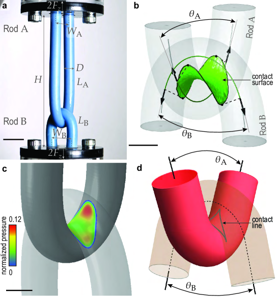
Figure 1: The orthogonal clasp: two rods in physical contact. a, Photograph of an elastic orthogonal clasp: two homogeneous rods (A and B) lying in orthogonal planes are brought into contact. Both rods have a rest diameter $D$, respective rest lengths $L_{\text{A}}$ and $L_{\text{B}}$ and their extremities are fixed at distances $W_{\text{A}}$ and $W_{\text{B}}$ apart. The loading is performed by varying the wall-to-wall distance $H$. Scale bar: 20 mm. b, Tomographic rendering of the elastic clasp in the vicinity of the contact surface obtained from $\mu$CT. The physical centerlines of the rods are represented as thin dark gray tubes. The local opening angles of the two rods, $\theta_{\mathrm{A}}$ and $\theta_{\mathrm{B}}$, are defined as the angle between the two tangents (black arrows) to the respective centerlines at the extremities of the (green) portions of the centerline attributed to the contact (or green) surface. Scale bar: 5 mm. c, Corresponding FEM computation of the elastic orthogonal clasp for the same parameters as in b. The colormap represents the contact pressure distribution (normalized by $EA/D^{2}$) between the two rods. Scale bar: 5 mm. d, Equilibrium configuration of an ideal orthogonal clasp with two perfectly flexible tubes in contact. The tubes have circular cross-sections orthogonal to the centerline. The idealized contact set is a closed, curvilinear diamond-shaped, line, meaning that there is a gap region between the tips of the two tubular surfaces. All configurations in a-c were obtained for the same physical parameters: $D=8.5$ mm, $L_{\mathrm{A}}=170$ mm, $W_{\mathrm{A}}=17$ mm, $L_{\mathbf{B}}=63.7$ mm, $W_{\mathrm{B}}=17$ and $H=103.2$ mm. The ideal clasp in d was computed for the opening angles, $\theta_{\mathrm{A}}$ and $\theta_{\mathrm{B}}$, measured on the elastic clasp of a-c ($\theta_{\mathrm{A}}=58^{\mathrm{o}}$ and $\theta_{\mathrm{B}}=33^{\mathrm{o}}$).

Contact surface of the elastic orthogonal clasp

Fig. 1a presents the experimental setup that we designed to study elastic orthogonal clasps systematically. We clamp two homogeneous elastic rods, rod A and rod B, to two rigid walls, the distance between which ($H$) is varied to bring the rods into contact. The two rods have equal rest diameters $D$, respective rest lengths $L_{\text{A}}$ and $L_{\text{B}}$, and their extremities are clamped at distances $W_{\text{A}}$ and $W_{\text{B}}$ apart. As the imposed wall-to-wall distance $H$ is varied, the overall geometry of the elastic clasp changes. Each wall applies a total vertical force of $2F_{z}$ to the elastic clasp ($F_{z}$ per extremity). We define the normalized vertical force $f_{z}=F_{z}/EA$, where $E$ is Young’s modulus of the material and $A=\pi D^{2}/4$ is the unloaded rod cross-section area. The experiments enable us to investigate the contact geometry between the touching rods by analyzing the $\mu$CT volumetric images of tomographically scanned elastic clasps. To enable such a 3D image analysis, we customized a rod fabrication protocol (detailed in the SI text, Sec. 1.A) to produce (coaxial) composite rods. These rod designs, together with X-ray tomography, enabled the precise determination of the material centerlines of each rod, along with the contact-surface geometry between the rods.

In Fig. 1b, we show a representative example of a rendered three-dimensional $\mu$CT image of an elastic clasp along with rod centerlines and contact surface (see Methods, SI text, Sec. 1.B and Sec. 1.C). The saddle-shaped contact surface, physically hidden in between the two rods, is the primary object of our study. In parallel to our experimental investigation, we conducted full 3D simulations using the finite element method (FEM) to extract quantities that are not readily available from the experiment, with particular focus on the contact pressure between the rods (colorbar in Fig. 1c). In the SI text, Sec. 3, we detail our validation procedure of the FEM numerics using the force-displacement curves, $F_{z}(H)$, for the clasp configuration presented Fig. 1a. Beyond the precise localization of the saddle-shaped contact surface, our computational FEM procedure reveals a highly heterogeneous pressure field between the two rods, which we will analyze in detail. One of the central goals of our study is to rationalize the distribution of this pressure field using the geometrical theory of idealized orthogonal clasps.

The geometrical theory of idealized orthogonal clasps

The geometrical problem of predicting contact sets between tightly interwound filaments subject to a non-penetration constraint has been addressed previously in the context of ideal knot shapes, for example, Refs. [25, 26], where it was observed that it is common for double-contact lines to arise. Ideal shapes involve filaments that, by assumption, have undeformable, circular, orthogonal cross-sections of finite radius. Typically ideal knot problems are formulated as a purely geometrical problem with no mechanics, which corresponds to their centerlines being considered as inextensible yet perfectly flexible so that they can support no bending moment. Starostin [27] first considered the particular case of the ideal shape of an orthogonal clasp, but only for the four-fold symmetric case, where the two components are congruent. In our notation, Starostin assumed that the two opening angles (defined in  Fig. 1d) were equal $\theta_{\text{A}}=\theta_{\text{B}}$. In the Methods and the SI text, Sec. 4.D, we present a self-contained variant of Starostin’s analysis that allows for an explicit computation of the contact set (e.g., Fig. 1d), including the cases $\theta_{\text{A}}\neq\theta_{\text{B}}$, via the numerical solution of a set of ordinary differential equations. For each $0\leq\theta_{\text{A}},\theta_{\text{B}}<\pi$, the contact set is a closed, curvilinear diamond-shaped, line, which stands in contrast to the surface-patch contact set observed in both the experimental $\mu$CT and numerical FEM data for the elastic orthogonal clasp (where cross-sections are deformable); see Fig. 1b and c). A significant part of our study seeks to explain the connection between the contact patches observed for elastic orthogonal clasps and the contact lines predicted by the ideal orthogonal clasp model.

Double-contact lines arise in ideal knot shapes because at each arc-length along the tube centerline, the associated circular arc in the tube surface has two contact points with other surface arcs, each of which corresponds to another two distinct arc-lengths. This double-contact feature is found in the present case of the ideal orthogonal clasp, where the phenomenon is perhaps less surprising due to the presence of two planes of reflection symmetry. Moreover, due to the reflection symmetry, the set of all contact chords between two touching centerline points decomposes into a one-parameter family of closed equilateral tetrahedra. It is the one-parameter family of mid-points of these four tetrahedral edges that traces out the curvilinear diamond-shaped contact line. The corners of the diamond arise when the family of open tetrahedra collapses to two double-covered straight line segments. In turn, this coalescent limit arises at first and last contact points along the curve centerlines (or touch-down and lift-off points, cf. SI text Sec. 4.D for more detail). The diamond-shape contact line surrounds the two tips of the clasp equilibria, and consequently, there is an enclosed gap, or physical space, separating the two tubes close to their tips.

Heuristically, the connection between the contact lines of the ideal orthogonal clasp and the contact patches of the elastic orthogonal clasp can be explained, in both experiment and FEM, by cross-section deformation. Consequently, the idealized contact lines are, in reality, ‘fattened’ to become surface patches. In general, the deformation of the cross-sections can be sufficiently large that the gap between the tips of the ideal orthogonal clasp closes in the corresponding elastic orthogonal clasp. Nevertheless, in most cases, we do observe an overall resemblance between the shape of the ideal contact line and the boundary of the elastic clasp surface patch, as in Fig. 1b-d. And, as presented in Fig. 3b2, we observed one elastic clasp configuration in which the tip gap does persist. Furthermore, we will show below that in many cases, the pressure distribution in our FEM simulations of the elastic orthogonal clasp are highly concentrated on the diamond-shaped contact lines in the corresponding ideal orthogonal clasp and that these high pressures arise toward the boundary of the contact patch, with comparatively low contact pressures close to the central tip regions.

Opening angles of the elastic clasp

Next, we perform a quantitative comparison between the equilibria of the ideal and elastic orthogonal clasp configurations. To do so, we use the local opening angles $\theta_{\text{A}}$ and $\theta_{\text{B}}$, defined as the angle described by the tangents to centerlines of either the tube (for the ideal case) or rod (for the elastic case) at the touch-down and lift-off contact points (see Fig. 1b and 1d). Since these opening angles appear in both cases, we take them as the common denominator to identify corresponding equilibria in ideal and elastic orthogonal clasps. In the ideal orthogonal clasp, these two opening angles are the only model input parameters; the tube diameter and the magnitude of the tensions applied at the tube ends are scale factors. However, in the elastic orthogonal clasp, the two opening angles are observables rather than inputs. The inputs are the applied vertical load (or the vertical imposed displacement) and the displacement boundary conditions enforced at the ends of both rods. Still, for any elastic orthogonal clasp equilibrium configuration, the opening angles can be measured experimentally from the $\mu$CT data or computed as part of the FEM simulation. As we will discuss later, the opening angles are also of key importance when describing the frictional mechanics of touching filaments, as they reflect the extent of the contact region.

In Fig. 2a-d, we present four different configurations of displacement boundary conditions that we employed to explore a range of opening angles (the details of each configuration are provided in the caption of Fig. 2). The corresponding curves for $\theta_{\text{A}}$ and $\theta_{\text{B}}$, as functions of the normalized vertical load $f_{z}$, for these four configurations, are provided in Figs. 2e and f for experiment (datapoints) and simulation (solid lines). We note that the local opening angles computed using FEM are in excellent agreement with the experimental measurement. As expected, in all four cases, the opening angles of rods A and B decrease monotonically as $f_{z}$ increases; the clasp configurations become tighter.

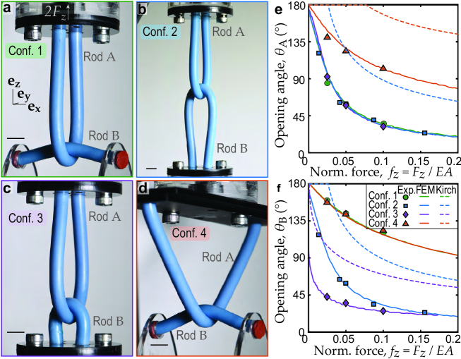
Figure 2: Opening angles of the elastic orthogonal clasp, as a function of applied load, for four specific configurations of displacement boundary conditions. a, The elastic rods of configuration 1 have the following normalized geometric attributes: rod A, $l_{\text{A}}=L_{\text{A}}/D=20$, $w_{\text{A}}=W_{\text{A}}/D=2$; rod B, $l_{\text{B}}=L_{\text{B}}/D=7.5$ and $w_{\text{B}}=W_{\text{B}}/D=7.5$ (rod B is straight when no load is applied). b, Configuration 2: rod A, $l_{\text{A}}=20$, $w_{\text{A}}=2$; rod B, $l_{\text{B}}=20$, $w_{\text{B}}=2$. c, Configuration 3: rod A, $l_{\text{A}}=20$, $w_{\text{A}}=2$; rod B, $l_{\text{B}}=7.5$, $w_{\text{B}}=2$. d, Configuration 4: rod A, $l_{\text{A}}=20$, $w_{\text{A}}=14$; rod B, $l_{\text{B}}=w_{\text{B}}=7.5$ (rod B is straight when load is applied). (Scale bars in a, b, c and d: 10mm.) e, Opening angles $\theta_{\text{A}}$ and f $\theta_{\text{B}}$ plotted versus the normalized applied vertical force $f_{z}$. The experimental opening angles (data points, measured through $\mu$CT tomography) and the FEM simulations (solid lines) are in excellent agreement. In all cases, the opening angles systematically decrease as the load $f_{z}$ increases. A simplified capstan computation of opening angles derived from a single elastic rod wrapped around a rigid straight cylinder in the absence of friction (dashed lines) delivers rather poor predictions.

Interestingly, the $\theta_{\text{A}}(f_{z})$ response is largely independent of the geometric conditions imposed on rod B and vice versa. Indeed, in configurations 1, 2 and 3, rod A has the same imposed boundary conditions; even though it is in contact with rods B of different lengths subject to different boundary conditions, it exhibits a nearly identical $\theta_{\text{A}}(f_{z})$ curve across these three configurations. Motivated by this observation, we sought to predict the opening angle response based on a simplified theory of a single Kirchhoff elastic rod wrapped around a rigid, right circular, cylinder of diameter $D$. Full details of this simplified theory are provided in the Methods and in the SI text, Sec. 4.A and Sec. 4.C. The Kirchhoff-based predictions, dashed lines in Fig. 2e and f, show a significant mismatch with the measured opening angles (experiments and FEM). We conclude that this simple theoretical approximation is inadequate, which will be consequential when we model the sliding clasp below.

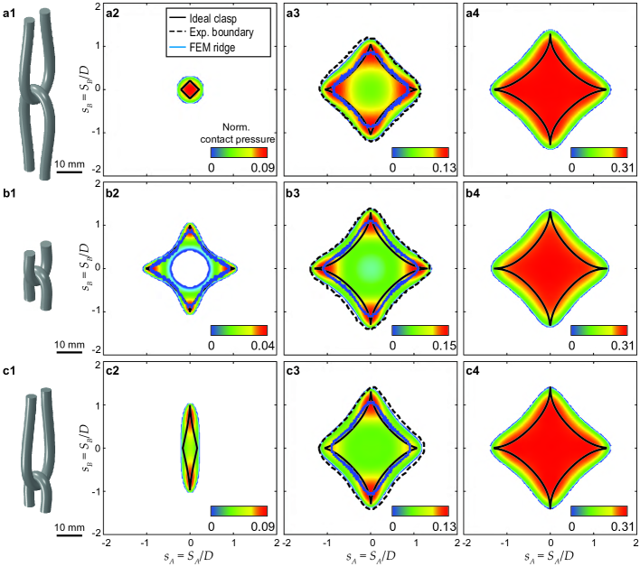
Figure 3: Contact pressure maps for nine different elastic orthogonal clasp equilibria. FEM-computed contact pressure fields of elastic orthogonal clasps subject to three different sets of geometrical boundary conditions at three different values of the applied load: (a1) $l_{\text{A}}=l_{\text{B}}=20$, b1, $l_{\text{A}}=l_{\text{B}}=7.5$, and c1, $l_{\text{A}}=20$, $l_{\text{B}}=7.5$ (with the three physical configurations illustrated corresponding to the applied load $f_{z}=0.005$). The pressure field data for different values of normalized load $f_{z}=\{0.005,\,0.05,\,0.15\}$ are presented in (a2, b2, c2), (a3, b3, c3), and (a4, b4, c4), respectively. (Blue solid lines): Ridges extracted from the FEM-computed pressure field. (Dashed lines): Experimentally observed boundaries of the contact surfaces. (Black solid lines): Prediction of contact curves from ideal orthogonal clasp theory.

The standard Kirchhoff rod model is based on the assumptions (or approximations) that cross-sections are undeformable and unshearable [28]. In the SI text, Sec. 2, we quantify the cross-section deformation, the centerline curvature, and the shear strain along the centerline of rod A, taking configuration 3 as a representative case. We observe that, even at the relatively low load $f_{z}=0.05$, all of these quantities reach substantial values in the neighborhood of contact. First, the cross-section can deform significantly, flattening from its original circular shape by up to 10 %. Secondly, the radius of the centerline curvature approaches the rod diameter. Finally, the shear strain reaches values up to 10 %. Therefore, in the elastic clasp, the Kirchhoff rod approximations are not accurate. Nevertheless, as we demonstrate below, the alternative one-dimensional geometric theory of the idealized orthogonal clasp does provide a framework to successfully rationalize the skeleton of the contact pressure distribution observed for the 3D elastic orthogonal clasp.

Distributions of the contact pressure

We proceed by analyzing the pressure distribution in the contact region of elastic orthogonal clasp. By way of example, we focus on the three representative cases of imposed boundary conditions shown in Fig. 3, each at three different values of the normalized applied loads ($f_{z}=\{0.005,\,0.05,\,0.15\}$). The three configurations considered are: a pair of long rods ($l_{\text{A}}=l_{\text{B}}=20$ and $w_{\text{A}}=w_{\text{B}}=2$; Fig. 3a1), a pair of short rods ($l_{\text{A}}=l_{\text{B}}=7.5$ and $w_{\text{A}}=w_{\text{B}}=2$; Fig. 3b1), and a combination of the long and short rods ($l_{\text{A}}=20$, $l_{\text{B}}=7.5$ and $w_{\text{A}}=w_{\text{B}}=2$; Fig. 3c1), where the physical configurations shown correspond to the low applied load $f_{z}\simeq 0.005$. For each of the nine cases, the contact pressure maps are computed using FEM simulation and then compared with both the extent of the corresponding contact surface patch measured from the $\mu$CT experiments, and the contact line predicted by the ideal orthogonal clasp analysis.

The contact pressure is computed from the FEM data as the normal force per unit area on the contact surface patch embedded in 3D. However, for visualization purposes, this scalar field is plotted as a color map in the 2D parameter space $(s_{\text{A}},\,s_{\text{B}})$; the arc lengths along the two rod centrelines provide a coordinate system for the contact surface patch (see Fig. 3a2-a4, b2-b4, and c2-c4). The point $s_{\text{A}}=s_{\text{B}}=0$ corresponds to the apices of the rods. With this parameterization, it is possible to overlay the boundaries of the contact region extracted from the $\mu$CT experiments of the elastic clasp configuration on the analogous FEM computations with the same opening angles (dashed lines); excellent agreement is found between the two. In these plots, we also juxtapose the contact line predicted by the ideal orthogonal clasp theory (solid black lines in Fig. 3a2-c2, a3-c3, a4-c4). All three equilibria for the first two sets of boundary conditions exhibit four-fold symmetric contact pressure maps $(\theta_{\text{A}}=\theta_{\text{B}})$. By contrast, there is only two-fold symmetry for the third configuration $(\theta_{\text{A}}\neq\theta_{\text{B}})$. The contact pressures are highly heterogeneous. For instance, Fig. 3c3 shows four pressure peaks near the entrance and exit regions of contact along the two rods, connected by ridges of high-pressure values (solid blue lines).

Remarkably, for all three cases of moderate loading $f_{z}\simeq 0.05$ presented in Fig. 3, the pressure ridges closely follow the curvilinear diamond-shaped contact line predicted by the ideal clasp geometric theory (solid black lines) for the same pair of opening angles; the four peaks in pressure are close to the four corners of the diamond. In these three cases, the purely geometric ideal clasp model provides an accurate skeleton of the pressure map in the physical system. Due to the deformability of the rod cross-sections, the singular, linear pressure field (force per unit length) predicted from geometry is smoothed out to yield the ridges in the surface pressure (force per unit area) for the elastic orthogonal clasp. In the case of higher loading ($f_{z}\simeq 0.15$; Fig. 3a4-c4), where there is significant deformation in the rod cross-sections, the surface pressure becomes more uniform over the interior of the region of contact, and the ridges are no longer observed.

The case of small loading ($f_{z}\simeq 0.005$; Fig. 3a2-c2) reveals a variety of contact pressure distributions depending on the global geometry of the equilibrium. Fig. 3a2 shows a highly localized pressure map, characterized by a single peak close to the apices $s_{\text{A}}=s_{\text{B}}=0$. However, in Fig. 3b2, both pressure ridges and a central region of vanishing pressure are observed, corresponding closely to the predictions of the ideal orthogonal clasp with its predicted gap between the tube surfaces close to the two centerline tips.

The hybrid long/short rod configuration in Fig. 3c2 exhibits a two-fold symmetric pressure corresponding to the asymmetry between rod A and rod B. There are two pressure peaks along rod B, separated by a saddle with low pressure between the apices. Even in this extreme case, the ideal clasp diamond contact line yields a reasonable prediction of the extent of the actual contact surface in the elastic orthogonal clasp.

The elastic clasp with sliding friction

Leveraging the physical understanding gained above for the elastic orthogonal clasp with negligible friction, we next impose a relative motion between two elastically deformable rods in a clasp configuration, with finite friction, to extend the problem to obtain the frictional sliding clasp. There is a direct analogy between this system and the capstan problem, in which one deformable filament is wrapped in a planar configuration around a rigid drum, or capstan. The classic Euler-Eytelwein version of this problem [29, 30, 21] assumes that the capstan is a rigid cylinder and that the filament is perfectly flexible, with a negligible radius of curvature compared to the radius of the capstan. Then, the maximal possible ratio of high tension $T_{1}$ at one end to low tension $T_{0}$ at the other end is predicted by the well-known capstan relation,

$$\frac{T_{1}}{T_{0}}=e^{\mu\varphi},$$ (1)

where $\varphi$ is the winding angle around the capstan, and $\mu$ is the friction coefficient (either static or dynamic depending on context) between the filament and the drum.

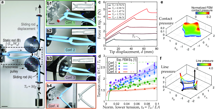
Figure 4: Friction-induced tension gain in the sliding elastic clasp. a, Experimental apparatus used to measure the tension ratio in different geometric configurations. Scale bar: 20 mm. b1-b4, Adaptation of configurations. 1, 2, 3 and 4 described in Fig. 2 to allow for the sliding of rod A around the static rod B. c, Experimentally measured upward force $T$ in the upper segment of the sliding rod A as a function of the upward displacement $d$ of the upper tip. d Ratio $K=T_{1}/T_{0}$ between the steady-state value of $T$ (plateau in c) and the value of the dead load $T_{0}$ applied to the lower end of rod A, plotted as a function of the normalized dead load $t_{0}=T_{0}/EA$, for the four different configurations. Experimental and FEM data are presented. The shaded regions correspond to the sensitivity of the FEM computation to the experimental uncertainty of the measured friction coefficient ($\mu=0.32\pm 0.03$). The horizontal dashed lines is the prediction from Eq. (1). e, Representative contact pressure map in the contact region obtained from the FEM simulation of configuration 3, at a normalized dead load of $t_{0}=0.05$ (the pressure is normalized by $EA/D^{2}$). f, Linear pressure map of the ideal clasp, where it can be computed analytically that for a maximum tension growth equilibrium, the linear pressure vanishes at the touch-down point (black circle), but has a singular Delta function at the lift-off corner (represented by a black arrow).

Our frictional sliding clasp load-displacement experiment can be viewed as a generalized capstan problem in which the static, rigid drum is replaced by a second deformable rod, thereby adding elastic deformation in a nontrivial way. Motivated by this analogy, we seek to measure the change in the tension between the two ends of a rod sliding in steady-state while wrapped around a second static but deformable rod. In our experiments (see Fig. 4a), rod A is guided by two frictionless pulleys to thread around the clamped rod B. The rods are surface-treated to ensure robust Amontons-Coulomb frictional behavior with $\mu=0.32\pm 0.03$ (see details in the SI text, Sec. 1.F). We measured the vertical force $T$ necessary to displace the upper extremity of rod A at a constant velocity subject to a dead load $T_{0}=Mg$, applied at the other extremity (where $M$ is the mass of dead weight and $g$ the gravitational acceleration). Upon pulling with a prescribed velocity, the measured tension $T$ first increases and then reaches a plateau value $T_{1}$ (see Fig. 4c and the Methods). We then quantify the steady tension ratio $K=T_{1}/T_{0}$ between the high and low-tension strands, as a function of the non-dimensional lower tension $t_{0}=T_{0}/EA$, for different geometric configurations. Specifically, we adopt the same four sets of imposed global geometric parameters as for the static elastic orthogonal clasp experiments, namely configurations 1 to 4 described in Fig. 2a-d), but with the presence of the pulleys instead of clamps for rod A (Fig. 4b1-b4). In the SI text, Sec. 4.B, we show that our long sliding rod (rod A) mainly carries an internal tensile force (i.e., parallel to the tangent of the rod centerline) far from the contact region with rod B.

In Fig. 4d, we plot the experimental tension ratio $K$ (data points) as a function of the dimensionless lower tension $t_{0}$ imposed by the dead load. We observe that all $K(t_{0})$ increase monotonically with $t_{0}$, albeit with significant differences for the various imposed geometrical configurations in either rod A or rod B. In parallel to the experiments, we carried out FEM numerical simulations of the steady-state frictional sliding elastic clasp (solid lines; see Methods, SI text, Sec. 3 for details of the simulations), finding good agreement with the experimental data (mean difference of $\approx 4.2\%$). The experimental and numerical data highlight the importance of the global opening angle imposed on the sliding rod; i.e. the angle between the tangents to rod A in the nearly straight regions far from contact, set experimentally by the distance between the pulleys. Note that the local opening angles cannot be accessed from $\mu$CT for these experiments. Indeed, we observe that $K(t_{0})$ is lower when the pulleys are far apart (configuration 4, orange triangles) than when they are close to each other (configuration 1, green circles). The overall ordering of this difference in tension ratio for varying global opening angle in rod A is correctly predicted in the capstan equation (1) when applied with the wrapping angle $\varphi$ interpreted as the global opening angle of rod A (dashed lines). However, the simple capstan equation interpreted in this way is inadequate to explain our data because it predicts that the tension ratio should be independent of both $t_{0}$ and the imposed geometry on the static rod B; neither of these predictions is close to being accurate. The mismatch between the capstan equation and our results stems from the non-trivial dependence of the local opening angles of the sliding and static rods on the applied tension $t_{0}$. Specifically, our results reveal the essential role of the static rod B; the tension ratio response is significantly larger when the static rod wraps further around the sliding rod. For example, the tension ratio of configuration 3 (where the static rod is initially short with ends close to each other) is larger than the tension ratio for configuration 1, by 21% at $t_{0}=0.05$.

The limitation of the simple capstan relation to predicting the data is consistent with the observation made above that a single elastic rod wrapped around a rigid cylindrical capstan is inadequate to accurately describe local opening angles of an elastic clasp configuration, and it is the local opening angles that are strongly related to the detailed contact mechanics that sets the maximal tension ratio $K(t_{0})$.

The detail of the contact region interactions, including sliding friction, can be further probed via FEM. In Fig. 4e, we plot the pressure field between the two rods for the frictional sliding clasp configuration of Fig. 4b3 (configuration 3). Just as in the static, frictionless case, the support of the contact pressure map in the presence of friction displays the familiar diamond shape, and again there are strong heterogeneities. Now, however, we observe only three pressure peaks in the $(s_{\text{A}},s_{\text{B}})$-plane; two at the extreme values of $s_{\textbf{B}}$, and one at the high-tension, or lift-off, end along $s_{\text{A}}$ where the pressure is largest. The symmetry along rod A is now broken, and the pressure at the touch-down end of the contact set is extremely low. As a first step towards understanding these qualitative features in the contact pressure distribution for the sliding elastic clasp, in the SI text, Sec. 4.F, we present a hybrid analysis of the ideal orthogonal clasp. In this framework, the shape of tube B is frozen to form a rigid tubular capstan with its own intricate geometry and local opening angle, around which the flexible tube A can reptate, with the contact set remaining identical with the static case (i.e., a closed, curvilinear diamond-shape line). In this idealized context, and as a consequence of moment balance on the finite radius flexible tube A, it can be derived (SI text, Sec. 4.E) that, in the presence of friction, the linear pressure distribution giving rise to the maximal possible tension ratio $K(t_{0})$ vanishes at the touch-down point, and has a Dirac delta function singularity at the lift-off point. Despite the strong simplifying assumptions in this model, these predictions for the linear pressure density, as illustrated in Fig. 4f, have a striking qualitative similarity to the surface pressure distributions as computed in the FEM simulations Fig. 4e.

Conclusions

Despite the apparent simplicity of having only two elastic filaments in contact, our experiments and FEM computations on the orthogonal clasp system have revealed highly nontrivial behavior. Specifically, we find that the contact pressure field between the two filaments is highly heterogeneous, with a curvilinear diamond ridge skeleton that can be explained qualitatively using a version of a primarily geometrical, one-dimensional theory for the ideal orthogonal clasp. The accuracy of this approximation for a wide range of loadings is all the more remarkable given the scale of the observed deformations of cross-sections in the two rods forming the elastic orthogonal clasp. Furthermore, a version of a V-belt capstan problem constructed from the ideal orthogonal clasp problem rationalizes the asymmetric roles of touch-down and lift-off points in the pressure distribution computed in the physical case when the two filaments are made to slide with respect to each other, in the presence of friction.

We hope that our findings will instigate future theoretical model developments that consider the intricate coupling of elasticity and contact geometry of filaments with a small but non-vanishing diameter. Future one-dimensional models should extend the geometric ideal tube description with the incorporation of elasticity, both through a bending stiffness for the centerline and in allowing cross-sectional deformation. Such efforts would significantly impact the homogenization schemes necessary to predictively describe more intricate networks of filaments such as knits, knots, and weaves, starting from the elastic clasp as a building block.

Methods

Fabrication of the rods for $\mu$CT imaging

For the static elastic orthogonal clasp experiment, elastomeric rods were fabricated through casting using silicone-based polymers, with a coaxial geometry comprising (i) a bulk core, (ii) a thin physical centerline fiber, and (iii) an outer coating layer. The bulk core was fabricated out of Vinyl PolySiloxane (VPS-16, Elite Double 16 Fast, Zhermack), whereas the physical centerline fiber and the outer coating were made out of the Solaris polymer (Smooth-On). The overall diameter of the resulting rod was $D=8.5$ mm. Additional fabrication details are provided in the SI text, Sec. 1.A.

X-ray micro-computed tomography ($\mu$CT)

Tomographic imaging of the elastic clasp configurations was performed using a $\mu$CT 100 (Scanco) machine for the static elastic orthogonal clasps in configurations 1 and 3, and an Ultra-Tom (RX-Solutions) machine for configurations 2 and 4. An in-house post-processing algorithm (written in MATLAB 2019b, MathWorks) was used to extract the coordinates of the centerline of the rods, as well as those of the rod-rod contact surface, from the volumetric $\mu$CT images (see SI text, Sec. 1.B).

Fabrication of the rods for mechanical testing

For mechanical testing, the rods were fabricated out of Vinyl PolySiloxane of two different grades: VPS-16 (Elite double 16 Fast, Zhermack) and VPS-32 (Elite double 32, Zhermack). The rods were cast in straight acrylic tubes of inner diameter $D=8$ mm. Further details are provided in the SI text, Section 1.E.

Mechanical testing

For the sliding orthogonal clasp experiment, we quantified the high-to-low tension ratio in the two ends of a rod sliding around another by performing force-displacement experiments on a mechanical testing machine (Instron 5943 with a 50 N load-cell). These tests used frictionless rotating pulleys to guide the sliding rod. The upper end of the sliding rod was pulled upward at constant velocity $U=3$ mm/s, while measuring the pulling force $T$. See further details in the SI text, Sec. 1.F.

Finite Element Modeling

Finite element method (FEM) simulations were performed using the software package ABAQUS/STANDARD to numerically compute the equilibria of the elastic static and sliding orthogonal clasps. The elastic rods were meshed with 3D brick elements with reduced integration and hybrid formulation (C3D8RH), with a Neo-Hookean hyperelastic material model. The geometry, meshing and loading sequences are detailed in the SI text, Sec. 3.

Bibliography

Bibliography

- Hardy et al. [2020] B. L. Hardy, M.-H. Moncel, C. Kerfant, M. Lebon, L. Bellot-Gurlet, and N. Mélard, “Direct evidence of neanderthal fibre technology and its cognitive and behavioral implications,” Sci. Rep. 10 (2020), 10.1038/s41598-020-61839-w.
- Buckner et al. [2020] T. L. Buckner, R. A. Bilodeau, S. Y. Kim, and R. Kramer-Bottiglio, “Roboticizing fabric by integrating functional fibers,” Proc. Natl. Acad. Sci. U.S.A. -, 202006211 (2020).
- Euler [1952] L. Euler, Methodus inveniendi lineas curvas maximi minimive proprietate gaudentes sive solutio problematis isoperimetrici latissimo sensu accepti, Vol. 1 (Springer Science & Business Media, 1952).
- Landau and Lifshitz [1986] L. M. Landau and E. M. Lifshitz, “Theory of elasticity,” Course of theoretical physics 7 (1986).
- Kirchhoff [1859] G. Kirchhoff, “Ueber das gleichgewicht und die bewegung eines unendlich dünnen elastischen stabes.” Journal für die reine und angewandte Mathematik 56, 285–313 (1859).
- Kirchhoff [1876] G. Kirchhoff, Vorlesungen über mathematische physik: mechanik, Vol. 1 (BG Teubner, 1876).
- Sano, Yamaguchi, and Wada [2017] T. G. Sano, T. Yamaguchi, and H. Wada, “Slip morphology of elastic strips on frictional rigid substrates,” Phys. Rev. Lett. 118, 178001 (2017).
- Goriely and Neukirch [2006] A. Goriely and S. Neukirch, “Mechanics of climbing and attachment in twining plants,” Phys. Rev. Lett. 97, 184302 (2006).
- Poincloux, Adda-Bedia, and Lechenault [2018] S. Poincloux, M. Adda-Bedia, and F. Lechenault, “Geometry and elasticity of a knitted fabric,” Phys. Rev. X. 8 (2018), 10.1103/physrevx.8.021075.
- Ayres, Martin, and Zwierzycki [2018] P. Ayres, A. G. Martin, and M. Zwierzycki, “Beyond the basket case: a principled approach to the modelling of kagome weave patterns for the fabrication of interlaced lattice structures using straight strips,” in Advances in Architectural Geometry 2018 (Chalmers University of Technology, 2018) pp. 72–93.
- Vekhter et al. [2019] J. Vekhter, J. Zhuo, L. F. G. Fandino, Q. Huang, and E. Vouga, “Weaving geodesic foliations,” ACM Trans. Graph. 38, 1–22 (2019).
- Baek et al. [2018] C. Baek, A. O. Sageman-Furnas, M. K. Jawed, and P. M. Reis, “Form finding in elastic gridshells,” Proc. Natl. Acad. Sci. U.S.A. 115, 75–80 (2018).
- Baek and Reis [2019] C. Baek and P. M. Reis, “Rigidity of hemispherical elastic gridshells under point load indentation,” J. Mech. Phys. Solids 124, 411–426 (2019).
- Yamaguchi, Onoue, and Sawae [2020] T. Yamaguchi, Y. Onoue, and Y. Sawae, “Topology and toughening of sparse elastic networks,” Phys. Rev. Lett. 124, 068002 (2020).
- Stoop, Wittel, and Herrmann [2008] N. Stoop, F. K. Wittel, and H. J. Herrmann, “Morphological phases of crumpled wire,” Phys. Rev. Lett. 101, 094101 (2008).
- Grason [2009] G. M. Grason, “Braided bundles and compact coils: The structure and thermodynamics of hexagonally packed chiral filament assemblies,” Phys. Rev. E. 79, 041919 (2009).
- Ward et al. [2015] A. Ward, F. Hilitski, W. Schwenger, D. Welch, A. W. C. Lau, V. Vitelli, L. Mahadevan, and Z. Dogic, “Solid friction between soft filaments,” Nat. Mater. 14, 583–588 (2015).
- Panaitescu, Grason, and Kudrolli [2017] A. Panaitescu, G. M. Grason, and A. Kudrolli, “Measuring geometric frustration in twisted inextensible filament bundles,” Phys. Rev. E 95, 052503 (2017).
- Panaitescu, Grason, and Kudrolli [2018] A. Panaitescu, G. M. Grason, and A. Kudrolli, “Persistence of perfect packing in twisted bundles of elastic filaments,” Phys. Rev. Lett. 120, 248002 (2018).
- Warren, Ball, and Goldstein [2018] P. B. Warren, R. C. Ball, and R. E. Goldstein, “Why clothes don’t fall apart: Tension transmission in staple yarns,” Phys. Rev. Lett. 120 (2018), 10.1103/physrevlett.120.158001.
- Maddocks and Keller [1987] J. H. Maddocks and J. B. Keller, “Ropes in equilibrium,” SIAM J. Appl. Math. 47, 1185–1200 (1987).
- Audoly, Clauvelin, and Neukirch [2007] B. Audoly, N. Clauvelin, and S. Neukirch, “Elastic knots,” Phys. Rev. Lett. 99 (2007), 10.1103/physrevlett.99.164301.
- Jawed et al. [2015] M. K. Jawed, P. Dieleman, B. Audoly, and P. M. Reis, “Untangling the mechanics and topology in the frictional response of long overhand elastic knots,” Phys. Rev. Lett. 115 (2015), 10.1103/physrevlett.115.118302.
- Patil et al. [2020] V. P. Patil, J. D. Sandt, M. Kolle, and J. Dunkel, “Topological mechanics of knots and tangles,” Science 367, 71–75 (2020).
- Gonzalez and Maddocks [1999] O. Gonzalez and J. Maddocks, “Global curvature, thickness, and the ideal shapes of knots,” Proc. Natl. Acad. Sci. U.S.A. 96 (1999).
- Carlen et al. [2005] M. Carlen, B. Laurie, J. H. Maddocks, and J. Smutny, “Biarcs, global radius of curvature, and the computation of ideal knot shapes,” in Physical and Numerical Models in Knot Theory and Their Application to the Life Sciences (World Scientific Publishing Co. Pte. Ltd., 2005).
- Starostin [2003] E. L. Starostin, “A constructive approach to modelling the tight shapes of some linked structures,” Forma 18, 263–293 (2003).
- Antman [2005] S. S. Antman, Nonlinear Problems of Elasticity (Springer, New York, 2005).
- Euler [1769] L. Euler, “Remarques sur l’effet du frottement dans l’equilibre,” Memoires de l’academie des sciences de Berlin -, 265–278 (1769).
- Eytelwein [1832] J. A. Eytelwein, Handbuch der Statik fester Körper: mit vorzüglicher Rücksicht auf ihre Anwendung in der Architektur, Vol. 1 (Reimer, 1832).