Investigating orientation effects considering angular resolution for a sample of radio-loud quasars using VLA observations

Abstract

1 Introduction

Quasars are the most luminous form of active galactic nuclei (AGNs), powered by the release of gravitational potential energy of material accreting onto the supermassive black holes at their centers. The axisymmetric nature of quasars makes orientation to the line of sight an essential quantity for comprehending their observed properties. Orientation plays a pivotal role in unifying not just type 1 and type 2 AGNs, e.g., Seyfert 1 and Seyfert 2 galaxies (Antonucci & Miller, 1985), but it is also fundamental in unifying classes of radio-loud quasars. When the radio jet axis of a quasar is aligned close to the line of sight , the core radiation gets Doppler-boosted and we observe a flat-spectrum radio-loud quasar, whereas, when the little Doppler-boosting takes place and we observe a steep-spectrum radio-loud quasar (Orr & Browne, 1982) dominated by the optically thin synchrotron radiation of the radio lobes. Properties of the optical spectra differ between these classes. The full width at half maximum (FWHM) of broad emission lines, such as $\mbox{H}\beta$, correlates with orientation:

Orientation not only governs classifications but also impacts the quantitative determination of fundamental properties like black hole mass and luminosity. The optical H$\beta$ line emitted from what is likely a flattened broad-line region is most commonly used to derive the mass of the black hole. As FWHM H$\beta$ correlates with the orientation (Wills & Browne, 1986), the derived mass is also orientation dependent (e.g., Runnoe et al. 2013a). Bolometric luminosity determination also depends on orientation (Nemmen & Brotherton, 2010). Face-on radio-loud quasars have brighter optical-UV continuum and X-rays (Jackson et al., 1989) and also the near-infrared emission is brighter by a factor of 2-3 (Runnoe et al., 2013b). This anisotropy needs to be understood, and ideally corrected for, in order to obtain the actual bolometric luminosity. Orientation also affects the luminosity functions of quasars (DiPompeo et al., 2014). For these reasons, orientation introduces scatter into the measurement of the fundamental properties of quasars. In order to fully understand the growth of black holes and their relationship to the evolution of galaxies, we require a better understanding and quantification of orientation, an essential parameter for axisymmetric quasars.

1.1 Orientation indicators for radio-loud quasars

Quasars are generally too distant to have their inner structure spatially resolved for direct measurements of their orientation (although see the amazing results for 3C 273 by the Gravity Collaboration et al. 2018 and for M87 by the Event Horizon Telescope Collaboration et al. 2019). However, radio-loud quasars have large-extent radio structures that can be used to determine orientation. The unresolved compact bases of these relativistic jets observed as cores undergo Doppler-boosting in the direction of motion (Orr & Browne, 1982; Wills & Brotherton, 1995; Van Gorkom et al., 2015). Hence, the core emission is orientation dependent and dominates in face-on quasars. Whereas, the isotropic diffuse emission from lobes dominates in the case of more edge-on quasars.

The core emission also depends on the power of the central engine. So to account for the power of the central engine, the core emission is normalized, often by the extended emission. Hence, the ratio of the flux density of the core to the extended emission at 5 GHz rest-frame is defined as the core dominance R (Orr & Browne, 1982), and serves as an orientation indicator. But using extended flux density to normalize the central engine power has its own shortcomings. First, extended emission includes the contribution from hotspots, which are formed when highly collimated jets hit material in the intergalactic (or intra-cluster) medium. Hence the extended flux density depends on the gaseous environment in which these quasars reside, which can differ from source to source and with redshift. Second, the extended emission is representative of the time-averaged power of the central engine, i.e., it depends on the history of the source and does not correspond to the current power, which governs the core emission.

Likely a better way to normalize the radio core is to use V-band optical luminosity because it is emitted from the contemporaneous accretion of material into the black hole whose rotation powers the jet. Therefore a better quasar orientation indicator is $\rm R_{V}$, the ratio of radio core luminosity and optical V-band luminosity (Wills & Brotherton, 1995; Van Gorkom et al., 2015). Evidence supporting the V-band optical luminosity as a better normalization factor includes its correlation with the emission-line luminosity (Yee & Oke, 1978) and the proportionality of jet power with the luminosity of the narrow-line region (Rawlings & Saunders, 1991). Although, the optical emission is anisotropic, between face-on & edge-on quasars, it varies only by a factor of about two, which is negligible in contrast to a factor of $\sim 10^{4}$ in the case of core flux density emission.

Other ways to determine core-dominance are as follows. Rawlings & Saunders (1991) uses luminosity of narrow-line region based on luminosities of [OII] and [OIII] lines to define $\rm R_{NLR}$. Willott et al. (1999) defines $\rm R_{OX}$ using total luminosity at 151 MHz to normalize the core luminosity. At this frequency, the total luminosity measures the luminosity of lobes.

Van Gorkom et al. (2015) performed two tests to determine the best orientation indicator among the four discussed above. The first test uses geometric rank as a proxy for orientation. Each object is assigned a rank as a sum of rank in ascending order of projected linear size and in decreasing order of the angle between the core and two hotspots. They found that only R and $\rm R_{v}$ shows high correlation with geometric rank. They also performed line regression to fit the data and calculate the data variance. They find that $\rm R_{v}$ has the lowest variance, i.e., optical luminosity introduces the least amount of scattering in the core-dominance parameter. They conducted another test by randomizing the normalization factor and obtained the distribution of the variance. They shuffled the denominator of each core dominance parameter by the value of the different source and obtained its variance against the best fit line calculated earlier. They repeated this 100,000 times to obtain a distribution of variance. They find that normalizing the core luminosity by a measurement from the same source only matters in the case of $\rm R_{v}$, when dividing by optical luminosity. Hence, their work confirms that $\rm R_{v}$ is a better orientation indicator, as previously claimed by Wills & Brotherton (1995). In this paper, we examine only the extended radio and the optical emission for normalization to determine core dominance.

1.2 Selection biases in past orientation studies

Few past orientation studies of radio-loud quasars have employed ideally selected samples. The widely used 3C/3CR catalog at 178 MHz, with a flux limit of 10 Jy, provides a nearly orientation-independent sample, as at this low frequency the emission is dominated by the extended optically thin component. But, the high-flux limit makes this catalog biased towards high-luminosity sources, which may not be typical. Orr & Browne (1982) use a flux-limited sample of 3C quasars, with no redshift constraints, to study their radio core dominance R. Their results on the quasar counts indicate that samples selected at high-frequencies, above 1 GHz, have more high-redshift quasars in comparison to samples selected at lower frequencies of a few hundred MHz. High-redshift quasars will go through higher Doppler-boosting and will have flatter spectra on average. Hence the sample will be biased towards flat-spectrum quasars.

On the other hand, an optical magnitude limit also introduces a bias towards flat-spectrum radio quasars (Jackson & Browne, 2013; Kapahi & Shastri, 1987). For e.g., the Wills & Browne (1986) sample is a collection of quasars from different catalogs based on their optical brightness cutoff ($<$17 mag) and a redshift cutoff of 0.7. The anti-correlation between R and optical magnitude (Browne & Wright, 1985) means that quasars with jet close to the line of sight have enhanced optical emission. So, their sample includes quasars that are intrinsically fainter than 17 mag but optically beamed. The combination of magnitude, orientation, and redshift results in a sample that lacks faint quasars and is biased against low R quasars.

Runnoe et al. (2013a) studied the effects of orientation on determining the mass of black holes. Their sample consists of 52 radio-loud (RL) quasars from the RL subsample of Shang et al. (2011), excluding blazars. These objects have extended radio luminosities in a range of $\rm 26.5<log~{}L_{ext}<27.6$, measured at 5 GHz in units of $\rm erg~{}s^{-1}~{}Hz^{-1}$. Hence, the selected objects are similar in nature but differ by their orientation. For our sample, we performed a luminosity cut allowing range in $\rm L_{ext}$ down to 33.0 $\rm erg~{}s^{-1}~{}Hz^{-1}$ measured at a low frequency (325 MHz) that is dominated by emission from the lobe component.

1.3 Selection and resolution bias associated with FIRST

Recent studies are based on samples selected by matching Sloan Digital Sky Survey (SDSS, York et al. 2000) and Faint Images of the Radio Sky at Twenty-cm (FIRST, Becker et al. 1995) survey data. A sample selected at high frequency, such as 1.4 GHz in case of FIRST, is expected to be biased toward core-dominated quasars that have flat-spectra in comparison to the less orientation-biased lobe-dominated quasars that have steep-spectra.

Irrespective of the sample selection, it is quite common to use FIRST measurements to determine core dominance. Jackson & Browne (2013) claim that FIRST measurements, do not have the spatial resolution to reliably distinguish the core from more extended components. So the core flux densities obtained from the FIRST survey will therefore likely have excess flux density coming from the extended emission, thus overestimating the radio core dominance. Thus orientation studies based on FIRST survey radio data are biased by selection and resolution effects (e.g., Brotherton et al. 2015).

In order to improve the radio-core dominance measurements, we need high-resolution data that can separate core from extended emission. For instance, for radio data with 5$\arcsec$ resolution, we will not be able to distinguish a 1$\arcsec$ core from any extended emission within the resolution element. In the absence of high-resolution data, we would then likely over-estimate the core flux densities and poorly identify their orientation.

To test this idea, we proposed for NSF’s Karl G. Jansky Very Large Array (VLA) 10 GHz A-array observations of a well-selected and relatively orientation-unbiased sample of quasars. We selected 10 GHz because at this frequency: measurements are still efficient, and the cores will stand-out against extended emission. Using the A-array can achieve an angular resolution of 0.2”, a factor of 25 times smaller than FIRST. From our results, we have confirmed that high-resolution data (better than the $\sim$5$\arcsec$ of FIRST) is generally required to correctly estimate the core flux density of quasars.

The outline of this paper is as follows: Section 2 discusses the sample selection, followed by Section 3 about our VLA observations and the reduction procedures used to derive the core flux densities. We catalog all the radio and optical flux densities in Section 4. Next we define the two core dominance parameters, R and $\rm R_{5100}$ and the groups we determined on the basis of extended radio spectra in Section 5. Finally, we present our results in Section 6 followed by discussion and conclusion in Section 7 and Section 8. Appendix A shows the spectral energy distribution (SED) of our targets. Appendix B shows radio images of sources with resolved structure at 10 GHz in contrast to their point-like FIRST images. For our calculations we have used a cosmology with $\rm H_{0}=70~{}km~{}s^{-1}~{}Mpc^{-1}$, $\rm\Omega_{\Lambda}=0.7$ and $\Omega_{m}=0.3$. We have defined radio spectral index $\alpha$ by the relation: $\rm S_{\nu}\propto\nu^{\alpha}$, where S stands for the flux density and $\nu$ is frequency.

2 Sample selection

We used a relatively unbiased sample (Runnoe & Boroson 2020, ApJ submitted) that is likely largely representative of the full range of quasar orientations. These objects were selected from the Sloan Digital Sky Survey Data Release 7 (SDSS DR7) quasar catalog (Schneider et al., 2007) within a redshift range of $\mbox{0}.1<z<0.6$ to attain high-quality optical spectra for the measurements of the $\mbox{H}\beta$ emission line. The sample was then matched with the low-frequency 325 MHz Westerbork Northern Sky Survey (WENSS, de Bruyn et al. 2000; Rengelink et al. 1997), that has a resolution of ). WENSS covers the whole sky north of 30$\degree$, about 1/3 of the larger SDSS DR7 quasar catalog covering $\rm\approx 9380~{}deg^{2}$. A total radio luminosity cutoff $\rm log(L_{325})>33.0~{}erg~{}s^{-1}~{}Hz^{-1}$ was applied. This luminosity cutoff is generally above the WENSS flux limit of 18 mJy ($5\sigma_{rms}$) and also above the transition between Fanaroff-Riley class I and II sources at $\rm log(L_{325})\sim 32.5~{}erg~{}s^{-1}~{}Hz^{-1}$. At 325 MHz, the isotropic extended emission dominates in nearly every object and hence produces a quasar sample largely unbiased by orientation.

Core and lobe candidates were matched separately because each object may appear as separate entries in the WENSS catalog. Core candidates were matched within a search radius of $\rm 30\arcsec$, whereas lobe candidates were matched within $1100\arcsec$. To associate lobes with a core candidate three criteria were used; the two lobes should be within 30$\degree$ of being opposite to each other, their ratio of the distance from SDSS position should be within a factor of two and their flux ratio should also be within a factor of two. As a result, 142 sources were selected and visually inspected in SDSS, WENSS, FIRST and the NRAO VLA Sky Survey Catalog (NVSS, Condon et al. 1998) to ensure correct matching of all the components. Furthermore, 16 sources were removed based on visual inspection of the match at multiple wavelengths and a subsequent re-evaluation of the luminosity cut.

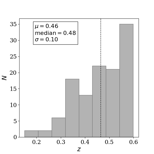
Figure 1:

3 VLA Observations and Data Reduction

The VLA continuum observations were carried out at 10 GHz (X-band) with the A-array configuration to achieve 0.2$\arcsec$ resolution, 25 times smaller than FIRST to separate the unresolved core from extended emission. We used the 3-bit digital samplers appropriate for X-band wideband observations with basebands of 2x2 GHz and a total bandwidth of 4 GHz. For both blocks, the flux calibrator was 3C 286. Each block included a scan of a phase calibrator at the beginning and the end. Some of our targets were already standard phase calibrators, so we also used them for phase calibration.

Data were reduced using the Common Astronomy Software Applications (CASA, McMullin et al. 2007) version 4.7.0. The initial 6 seconds of the data from each scan were flagged to take into account the stabilizing time for the array. We did not flag our data for shadowing, as A-array does not suffer from this effect. Antennas reported with bad baselines in the observer’s log were flagged wherever corrections were unavailable. By making plots of amplitude versus time for the flux calibrator we found that the spectral window 12 and 31 in the first block had an error, so we excluded these spectral windows while applying further calibrations.

The visibilities of the flux calibrator were modeled using the Perley-Butler 2013 (Perley & Butler, 2013) model for X-band. The initial phase calibration was performed to look for the time variation from scan to scan for the bandpass calibrator before deriving the bandpass solution. Then we solved for the antenna-based delay relative to the reference antenna. These phase and delay solutions were used to determine the bandpass solution that best determines the variation of the gain with frequency. Next, we derived the correction for the complex antenna gain for the flux calibrator and phase calibrators. The absolute flux densities of the phase calibrators were obtained assuming the gain amplitude for the phase calibrators is the same for the flux calibrator, for which we have taken the gain amplitude from the measured and modeled visibilities. The calibration solutions derived earlier were then applied to the flux and phase calibrators. We matched the targets to the neighboring phase calibrator and applied the solutions. Image synthesis was performed using the CLEAN task with multi-frequency synthesis imaging mode, Clark (1980), as the method of PSF calculation, and the Cotton-Schwab clean algorithm (Schwab, 1984) with one term and Briggs weighting (Briggs, 1995).

4 Essential radio and optical data

The newly synthesized 10 GHz images were visually inspected to ensure matching of the core position, i.e., the position of the pixel with maximum flux density, with the SDSS position. There were quasars with poor-quality images due to bad radio data that we dropped from further analysis. We used the CASA task imstat to measure the 10 GHz core flux densities from the peak flux density at the optical position. The standard deviations in the residual images produced by the CLEAN task provided the root mean square (RMS) noises.

Table 1 presents the properties of our final set of quasars. Column 1 and 2 lists the SDSS object names and their redshifts, respectively. We list the optical flux densities at 5100 Å in column 3, obtained from the SDSS spectra of these quasars. We adopted these measurements from Runnoe & Boroson (2020). They corrected the spectra for Galactic extinction.

Core flux densities at 10 GHz and 1.4 GHz are listed in columns 4 and 5 of Table 1, respectively. For the 1.4 GHz core flux densities we adopt measurements from Runnoe & Boroson (2020). They matched to the FIRST survey by manually determined the search radius. They visually determined the core and used the FIRST peak flux. For objects with core detections, they used the peak flux density as the core flux density. For twelve objects with no core detections they used the FIRST RMS and adopted a $\rm 5\sigma$ limit on the core flux density .

The extended, steep-spectrum emission in quasars dominates at MHz frequencies. So, to measure the extended flux densities and the spectral indices of extended emission, The radio spectral index of extended emission, $\alpha_{ext}$, is listed in column 10.

Table 1: SDSS names, redshifts, optical and radio flux densities, and spectral indices of extended emission of 119 radio-loud quasars.

Object name	Redshift	F5100	$\rm S^{core}_{10GHz}$	$\rm S^{core}_{1.4GHz}$	$\rm S_{WENSS}^{total}$	$\rm S_{TGSS}^{total}$	$\rm S_{7C}^{total}$	$\rm S_{VLSSr}^{total}$	$\rm\alpha_{ext}$	Group
SDSS	z		$(\rm mJy~{}beam^{-1})$	$(\rm mJy~{}beam^{-1})$	$(\rm mJy$)	$(\rm mJy$)	$(\rm mJy$)	$(\rm mJy$)
J073422.19+472918.8	0.382	9.67$\pm$0.25	12.39$\pm$0.06	6.47$\pm$0.14	766$\pm$31	991.9$\pm$99.8	1257$\pm$87	2020$\pm$300	-0.71$\pm$0.049	2
J074125.22+333319.9	0.364	19.38$\pm$0.22	8.61$\pm$0.03	3.01$\pm$0.22	1853$\pm$74	3683.1$\pm$261.3	2789$\pm$146	5330$\pm$470	-0.754$\pm$0.04	2
J074541.66+314256.6	0.461	96.02$\pm$0.12	449.8$\pm$0.42	614.64$\pm$0.15	3458$\pm$138	6802$\pm$484.7	5948$\pm$296	15370$\pm$1340	-0.716$\pm$0.045	2
J075145.14+411535.8	0.429	5.24$\pm$0.29	94.16$\pm$0.41	202.68$\pm$0.14	460$\pm$19	533.3$\pm$53.6	457$\pm$48	730$\pm$100	-0.748$\pm$0.105	3
J080413.87+470442.8	0.510	2.30$\pm$0.29	107.5$\pm$0.43	847.18$\pm$0.21	2574$\pm$103	4586.6$\pm$459.5	3644$\pm$184	3720$\pm$450	-0.64$\pm$0.049	2f
J080644.42+484149.2	0.370	23.09$\pm$0.27	81.08$\pm$0.25	43.32$\pm$0.14	3099$\pm$124	6867.8$\pm$519	6071$\pm$298	1210$\pm$160	-0.766$\pm$0.044	2
J080754.50+494627.6	0.575	2.65$\pm$0.29	1.7$\pm$0.02	1.05$\pm$0.21	1452$\pm$59	3061.4$\pm$306.5	2787$\pm$157	5000$\pm$630	-0.897$\pm$0.051	2
J080814.70+475244.7	0.546	14.00$\pm$0.26	3.26$\pm$0.03	26.39$\pm$0.15	226$\pm$11	365.4$\pm$41.9	610$\pm$76	540$\pm$100	-0.827$\pm$0.08	2

Note. — Table 1 is published in its entirety in the machine readable format. A portion is shown here for guidance regarding its form and content.

5 Core dominance determinations

We derived two radio orientation indicators: (1) R, radio core dominance, defined as the ratio of the observed core flux density and the observed extended flux density k-corrected to 5 GHz rest-frame (equation 1), (2) $\rm R_{5100}$ defined as the ratio of the core flux density and the optical 5100 Å flux density (equation 2).We derive both orientation indicators using core flux densities at observed frequencies, $\rm\nu_{obs}$, of 1.4 GHz (from FIRST) and 10 GHz.

$$\rm R_{\nu_{obs}}=(S_{\nu_{obs}}^{core}/S_{obs}^{ext})|_{5GHz,rest}$$ (1)

$$\rm R_{5100,\nu_{obs}}=S_{\nu_{obs}}^{core}/S_{5100\text{\AA}}$$ (2)

The flux densities ($\rm S_{obs}$) observed at frequency $\rm\nu_{obs}$ are k-corrected to 5 GHz rest-frame using

$$\rm S_{5\rm GHz,rest}=S_{obs}~{}(1+z)^{-(1+\alpha)}\left(\frac{5\rm~{}GHz}{\nu_{\rm obs}}\right)^{\alpha},$$ (3)

where, z is the redshift and $\alpha$ is the radio spectral index. We assumed the radio spectral index of the cores to be zero, as quasar cores have flat-spectra (Bridle et al. 1994, Kimball et al. 2011), so, $\rm S^{core}_{5GHz,rest}=S^{core}_{\nu_{obs}}/(1+z)$. The observed extended flux density is the difference of total flux density at the observed frequency ($\rm\nu^{\prime}_{obs}$) and the core flux density at the observed frequency ($\rm\nu_{obs}$) i.e. $\rm S^{ext}_{obs}=S^{total}_{\nu^{\prime}_{obs}}-S^{core}_{\nu_{obs}}$. To calculate $\rm S^{ext}_{5GHz,rest}$, we need to measure the extended radio spectral index, $\alpha_{ext}$.

The best way to calculate $\rm\alpha_{ext}$ is to fit a power-law slope to the total flux densities obtained from simultaneous observations at two low radio frequencies, where the emission is dominated by the lobes. In practice, observations are not available at low enough frequency and one still needs to know whether an object is core-dominated or lobe-dominated. If an object is core-dominated, total flux density will be dominated by the core emission rather than the lobe emission, giving an inaccurate measure of $\rm\alpha_{ext}$. So, to determine the most accurate $\alpha_{ext}$ we plotted the radio spectral energy distribution (SED) of our targets. We plotted the total flux densities from , TGSS, 7C, WENSS, NVSS, and FIRST. . We also included the core flux densities from FIRST and the new 10 GHz observations (Appendix A). By visually inspecting these radio SEDs we were able to distinguish flat-spectrum sources (core-dominated) from the steep-spectrum sources (lobe-dominated).

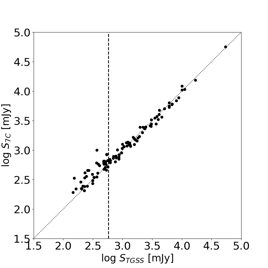
Figure 2: The total flux densities from 7C (y-axis) versus TGSS (x-axis) in log scale. The dotted line represents the 1:1 ratio and the dashed line represents the cut at below which we disregard TGSS values as they suffer from missing extended components.

For a significant number of quasars, we found that the total flux densities from TGSS were falling below the overall slope (eg., J080814.70+475244.7, J080833.36+424836.3, J085341.18+405221.7, J110313.30+301442.7, etc.). This is the reason why we included the 7C survey in our analysis, despite being at a frequency so close to that of TGSS. Figure 2 compares the total flux densities from TGSS and 7C in log scales. The plot shows an agreement between the two surveys only for . The difference between TGSS and 7C at lower flux densities is because of the resolution bias, 7C having a larger beam of 70$\arcsec$. The ratio of flux densities of the two surveys matches to almost unity for sources brighter than 2 Jy (see section 4.5 of Intema et al. 2017). We therefore made a cut at and discarded TGSS measurements that are below the cut while plotting radio SEDs. The total flux densities between WENSS, 7C, TGSS and VLSSr agree well with a consistent power-law in a majority of our sources.

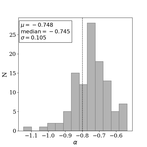
Figure 3: Histogram of $\rm\alpha_{ext}$ measured from the slope of the best-fit line to the radio spectra of quasars in group 2 and group2-flag, that are possibly lobe-dominated quasars. The dashed line at $-0.8$ represents the typical value for $\rm\alpha_{ext}$ (Kimball et al. 2011, Kimball & Ivezić 2008). The mean of our sample lies nearby at $\rm\alpha_{ext}=-0.748$.

We measured $\rm\alpha_{ext}$ by fitting a slope to the radio spectra between 150 MHz and 1.4 GHz including total flux densities from , TGSS, 7C, WENSS, and NVSS. Although being at 1.4 GHz, NVSS flux density for core-dominated objects is contaminated by core emission (eg., J084957.97+510829.0, J123413.33+475351.2, etc.) and not ideal for $\rm\alpha_{ext}$ measurement, it can be used for lobe-dominated objects as it follows the overall extended slope. We included NVSS so that we can measure $\rm\alpha_{ext}$ for targets that do not have 7C, TGSS and observations. NVSS also served as an reference point along with WENSS in the SEDs to identify the resolution bias in TGSS for fainter targets. We used the measured $\rm\alpha_{ext}$ to differentiate between core-dominated, lobe-dominated, and intermediate quasars. Only for the lobe-dominated quasars, we use the measured value of $\rm\alpha_{ext}$ for our calculations. For core-dominated and intermediate quasars we use the sample mean of $\rm\alpha_{ext}$.

On the basis of $\rm\alpha_{ext}$ and its error we divided our sample into three groups and one sub-group. Group1 consists of sources with flat radio spectra over 150 MHz to 10 GHz, indicating they are likely core-dominated quasars. Group2 consists of sources with $\rm\alpha_{ext}$ steeper than $-$0.5 and very small errors. These sources are likely lobe-dominated quasars. Figure 3 shows the distribution of $\rm\alpha_{ext}$ in the quasars of Group2 and Group2-flag and shows a mean $\rm\alpha_{ext}$ of . Finally, Group3 consists of sources with $\rm\alpha_{ext}$ flatter than $-$0.5 and errors greater than 10%. These sources are likely intermediate between core and lobe-dominated quasars.

For Group2 and Group2-flag, we calculated $\rm S_{obs}^{ext}$ taking the difference between the total flux densities at $\nu^{\prime}_{obs}=325$ MHz (from WENSS) and core flux densities at $\nu_{obs}=$ 1.4 GHz (10 GHz). We used the measured $\rm\alpha_{ext}$ to k-correct the extended flux density to the 5 GHz rest-frame (equation 3) and calculated $\rm R_{1.4GHz}~{}(R_{10GHz})$ using equation 1. For Group1 and Group3, consisting of quasars that are likely core dominated, we ideally needed simultaneous measurement of core and total flux density to calculate the extended flux density. Therefore, we used the difference between the FIRST total and core flux densities to measure $\rm S_{obs}^{ext}$. We used the mean $\alpha_{ext}$ of the rest of our sample, i.e., $-$0.748 (Figure 3), to k-correct the extended flux densities to 5 GHz rest-frame. Table 2 lists the logarithm of radio core dominance evaluated at $\nu_{obs}$ of 1.4 GHz (log $\rm R_{1.4GHz}$) and 10 GHz (log $\rm R_{10GHz}$) in column 3 and column 4, respectively. We used the 5100 Å flux densities to normalize the radio core flux densities at the same $\nu_{obs}$. The log $\rm R_{5100,1.4GHz}$ and log $\rm R_{5100,10GHz}$ are given in columns 5 and 6.

Table 2: Logarithm of $\rm R$ and $\rm R_{5100}$ calculated using new 10 GHz and FIRST 1.4 GHz core flux densities.

Object name	log($\rm R_{1.4GHz}$)	log($\rm R_{10GHz}$)	log($\rm R_{5100,1.4GHz}$)	log($\rm R_{5100,10GHz}$)
J073422.19+472918.8	-1.33$\pm$0.056	-1.04$\pm$0.052	1.89$\pm$0.034	2.17$\pm$0.026
J074125.22+333319.9	-2.00$\pm$0.084	-1.54$\pm$0.042	1.25$\pm$0.074	1.71$\pm$0.012
J074541.66+314256.6	0.07$\pm$0.046	-0.09$\pm$0.046	2.87$\pm$0.001	2.73$\pm$0.002
J075145.14+411535.8	1.26$\pm$0.043	0.93$\pm$0.043	3.65$\pm$0.055	3.32$\pm$0.055
J080413.87+470442.8	0.34$\pm$0.049	-0.72$\pm$0.050	4.63$\pm$0.124	3.73$\pm$0.124
J080644.42+484149.2	-1.04$\pm$0.046	-0.77$\pm$0.046	2.33$\pm$0.012	2.61$\pm$0.012
J080754.50+494627.6	-2.25$\pm$0.206	-2.04$\pm$0.052	1.66$\pm$0.228	1.87$\pm$0.109

Note. — Table 2 is published in its entirety online in machine readable format. A portion is shown here for guidance regarding its form and content.

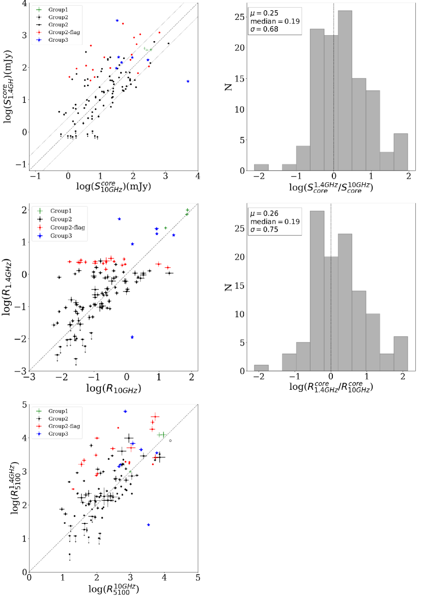
Figure 4: The left panels show scatter plots of core flux density measured at 1.4 GHz and 10 GHz and the corresponding R and $\rm R_{5100}$ measurements on log scales. The points are color coded according to the groups defined by the radio spectra of their extended emission. Points on the bottom left corner panel with downward arrows represent the objects with FIRST flux limits. The dashed lines show where the two quantities are equal. Top left: A scatter plot with the logarithm of 1.4 GHz core flux density on y-axis and the logarithm of 10 GHz core flux density on the x-axis. The dotted line represents $\rm y=x\pm 0.43$, an estimate of the $1\sigma$ scatter introduced by the core variability. Middle left: scatter plot of log R calculated from the 1.4 GHz FIRST cores on the y-axis and from the 10 GHz cores on the x-axis normalized by the extended flux densities scaled to 5 GHz rest-frame according to the groups as discussed in section 5. Bottom left: scatter plot of $\rm R_{5100}$ values calculated from the ratio of 10 GHz vs 1.4 GHz core flux densities and 5100Å flux density. The point with black open circle () represent a quasar with a bad 5100 Å flux density measurement. Right: panels show the histograms of the corresponding ratio of the quantities in the x and y axis of the left panels. The dashed lines in these histograms show where the ratios are equal.

6 Results

Figure 4 compares the core flux densities at 1.4 GHz (from FIRST) and 10 GHz (top panel) and their impact on the determination of the radio core dominance, R (middle panel) and $\rm R_{5100}$ (bottom panel). The radio cores of quasars typically have a flat spectrum over a broad range of frequencies, so we expect that the core flux density at the FIRST and the observed frequencies to be the same. There are three factors that can introduce differences: variability, inverted core spectrum, and insufficient resolution.

The scatter plot of 1.4 GHz vs 10 GHz core flux densities provides a path to statistically estimate the core variability for our sample. The objects below the 1:1 line have 10 GHz core flux density larger than the 1.4 GHz flux density (except the points with arrows that represent the FIRST detection limit). This increase in the core flux density is likely due to core variability. In order to quantify the variability level, we plot the histogram of the logarithm of the ratio of the two flux densities on the top right panel of Figure 4. The distribution is asymmetric around the dashed line representing equal fluxes. . The core variability contributes to the negative tail of the distribution. .

The assumption of a flat radio core spectra could introduce scatter around the 1:1 line that represents $\rm\alpha_{core}=0$. Hovatta et al. (2014) found the mean $\rm\alpha_{core}=0.22\pm 0.04$ for a sample of 133 flat-spectrum radio quasars using VLBA observations. Their mean core spectral index also shows an anti-correlation with the linear size of the core, implying that the measurements for high-redshift sources were contaminated by the jet emission. To quantify the effect of inverted core spectral index we generated 10,000 samples of $\rm\alpha_{core}$ from a Gaussian distribution with a mean of 0.22 and standard deviation of 0.04 and calculated the mean flux density of the sample scaled between 1.4 GHz and 10 GHz. We found that the change in flux density is a factor of 1.54 due to non-zero core spectral index. This is the largest effect that could be induced due to an inverted core spectral index which is still smaller than the apparent factor of resulting from core variability.

The scatter plot of 1.4 GHz vs 10 GHz core flux densities also shows that majority of our targets are above the 1:1 dashed line, indicating that many core measurements are contaminated by poorly resolved extended emission. We found objects for which FIRST fluxes are above the dotted line representing the core variability limit In a few of them we have detected extended features in the 10 GHz images at the scale of a few arcseconds or less (see Appendix B).

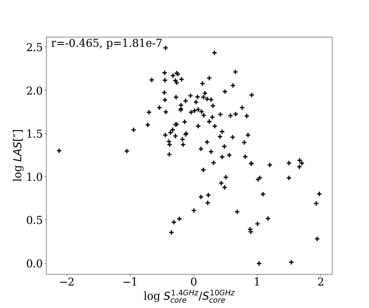
Figure 5: An anti-correlation between the ratio of the flux densities at 1.4 GHz (from FIRST) and 10 GHz (x-axis) vs the largest angular size (LAS) (in units of arcseconds) from FIRST in log-log scale (y-axis). Pearson’s correlation coefficient is r = $-$0.465 corresponding to a probability that these quantities are uncorrelated of 1.81e-7.

If the FIRST core measurements are contaminated by the extended emission, we expect larger contamination as the angular size of the target in FIRST image decreases. Figure 5 plots the largest angular size (LAS) from FIRST against the ratio of flux densities at 1.4 GHz (from FIRST) and 10 GHz in log-log scale. The largest angular size were taken from Table 1 of Runnoe & Boroson (2020). It was determined by plotting the FIRST elliptical Gaussian fits to all components associated with a source and calculating the largest associated size scale among them. We find that the ratio increases as the FIRST angular size decreases. The anti-correlation has a Pearson’s r-coefficient of -0.465.

These results clearly demonstrate that the cores were unresolved at the FIRST resolution and their core flux density measurements were contaminated with extended emission. With our new X-band observations, we were able to resolve these sources and hence improved the core flux density measurements.

Since the core flux densities were systematically higher in the case of the FIRST measurements, we expect the radio core dominance calculated from the FIRST survey to have higher values too. Figure 4 (middle panel) compares R using the FIRST core and 10 GHz core measurements and shows a prominent excess. We observed the same excess in the $\rm R_{5100}$ in figure 4 (bottom panel) while using FIRST core measurements. We have plotted the error bars accounting for uncertainties in flux densities and $\alpha_{ext}$.

Our results confirm the Jackson & Browne (2013) claim about resolution effects, and that radio core dominance calculated from FIRST maps is often compromised and biased high. With our current high-resolution radio images, we have determined improved core flux densities and hence improved the radio orientation indicators R and $\rm R_{5100}$.

7 Discussion

There are a number of choices to make when determining the radio core dominance of a quasar. Observations are conducted at a particular frequency and resolution given available facilities and/or surveys. There are distinctly different issues when it comes to measuring radio core flux density compared to that of the total or extended radio emission.

The radio core stands out against extended emission best at higher frequencies, making 10 GHz a better choice compared to lower frequencies. Similarly, radio cores are better distinguished from extended emission at higher angular resolution. These considerations make our choice of VLA A-array 10 GHz observations among the best to measure quasar radio cores. As previously discussed, the FIRST Survey using the VLA at B-array and 1.4 GHz suffers shortcomings that can compromise the results for individual objects.

Figure 6: TGSS, FIRST and VLA 10 GHz images (see Table 3 for image statistics) of two known CSS sources in our sample that are either (a) resolved or (b) unresolved at 10 GHz. In both cases the contamination of core flux density due to extended emission is removed in the 10 GHz observation. Their SEDs show VLSSr flux density (at 74 MHz) falls below the steep slope, expected in case of CSS quasars.

In the future, surveys like the VLA Sky Survey (VLASS) will provide a better source of archival core flux densities than the FIRST. VLASS will cover the entire sky above $-$40 degrees at 2-4 GHz with a resolution of 2.5 arcsec (Lacy et al. 2019). This will provide the radio cores at double the frequency and resolution of the FIRST. There may still be issues of core contamination, but they will be much reduced, although A-array 10 GHz observations remain the optimal choice when possible.

Even after making the best choices for measuring radio cores, our measurements are affected by intrinsic core variability. The cores exhibit a variability factor of up to about two over timescales of a few years (Barthel et al. 2000, Verschuur et al. 1988). Our 10 GHz VLA and FIRST measurements are separated by years to decades, as the FIRST survey includes observations from 1993 to 2011; our measurements are affected by variability too. Our analysis suggests that the quasars in our sample have variability of about a factor of two and a half over the time period considered. This is true for both core-dominated and lobe-dominated quasars. Approximately two fifths of our sample shows excess core flux density in FIRST measurements beyond the amount ascribable to variability. Hence, our results demonstrate statistically that the contamination of FIRST core measurements by the extended emission is apparent, as discussed by Jackson & Browne (2013).

Also important in the determination of radio core dominance is the choice of the normalization factor. We have reported radio core dominance measurements by normalizing the radio cores by both the extended radio flux density and the optical. The optical normalization of $\rm R_{5100}$ is preferred. Wills & Brotherton (1995) first defined an alternative way to normalize core luminosity by the V-band optical luminosity as a measure of intrinsic jet power. They claimed that $\rm R_{V}$ is a better orientation indicator than R, as it shows a better correlation with the jet angle and FWHM $\rm H{\beta}$ compared to the more traditional $\rm R$. While the optical continuum likely has an orientation dependence (e.g., Nemmen & Brotherton 2010), it is relatively small compared to the variation in radio cores seen within the beaming angle. The optical luminosity is also representative of the power of the AGN at the present epoch, while the extended radio emission represents some time averaging of the power of past activity. The extended radio luminosity is also affected by the jet’s interaction with the environment, introducing additional scatter. Van Gorkom et al. (2015) presents a comparative study of several different radio-based radio core dominance normalizations, using complementary tests, also finding the optical continuum a superior normalization choice.

The extended radio flux density normalization of $\rm R$ is laborious. Low frequency observations are preferred since extended emission has a steep spectrum compared to the relatively flat spectrum of cores. We adopted the WENSS total flux density at observed-frame 325 MHz. Even lower frequency observations would be better in principle, as the degree of core contamination will be increasingly negligible, although there are other considerations. The TGSS at 150 MHz is the highest resolution and sensitivity radio survey available for obtaining the total flux density measurements. It has a resolution of 25$\arcsec$ at which the extended emission may be resolved. Therefore, the search radius to match lobe candidates should be carefully chosen to make sure that all components are collected, otherwise one may end up underestimating the flux densities. Using lobe matching technique that Runnoe & Boroson (2020) performed for WENSS, could be very taxing for TGSS as a search radius of 1100$\arcsec$ would result in a large number of detection to match to a core. Another downside with TGSS is that it suffers with a resolution bias. It has a higher resolution power but a poor low surface brightness sensitivity. This leads to lower total flux densities for objects fainter than 2 Jy when compared to a lower resolution survey like 7C (Intema et al., 2017). Although, for our sample we found this threshold to be $\sim 580$ mJy by comparing with 7C survey. Plotting SEDs with total flux densities from other low resolution surveys like WENSS and NVSS shows that 7C measurements comply with the overall trend, whereas TGSS measurements for the fainter objects fall below because of the resolution bias. For a small set of objects, TGSS is the preferred survey for extended flux densities given that the objects are bright enough and the matching is done carefully. For a large set of objects, this would be difficult, in which case WENSS falls at the sweet spot of frequency and resolution good for extended flux density measurements. Several orientation studies used NVSS extended flux densities as it is at the same frequency as the FIRST. Being at 1.4 GHz, the NVSS total flux density is often beamed and suffers from core variability, hence is not a good choice for normalization.

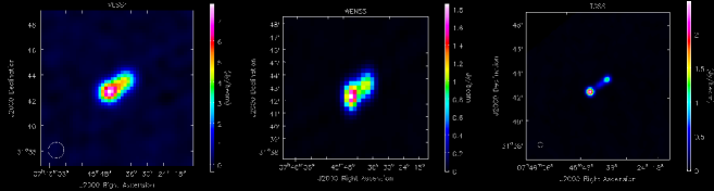
Figure 7: Radio maps of J074541.66+314256.6 from VLSSr, WENSS and TGSS demonstrating their resolving power.

The extended flux densities needs to be k-corrected (Hogg et al. 2002) and scaled to 5 GHz for the measurement of R. When using low frequency data like from TGSS and WENSS, $\alpha_{ext}$ should be choosen carefully. As the frequency difference is very large, a small change in $\alpha_{ext}$ can significantly affect your R measurements. We took the approach of determining the extended slope for individual objects by fitting their SEDs from TGSS, 7C, WENSS, and NVSS (Appendix A). In lobe-dominated quasars this gives a fair measurement of the radio spectral index for extended emission and we can account for variability concerns separately. For core-dominated sources, $\alpha_{ext}$ is not well measured in this way and requires simultaneous measurements. So, we adopted the mean spectral index of our sample for them.

The actual utility of radio core dominance is as an indicator of the orientation of the radio jet to the line of sight, and it is desirable to be able to relate it to a physical angle. Marin & Antonucci (2016) provide such a quantitative prescription, deriving a semi-empirical function between core-dominance and inclination angle by numerically fitting a polynomial regression relation to sources within a equally distributed solid angle. Their relation provides a measurement of inclination from log R of radio-loud AGNs with an accuracy of $\approx 10^{\degree}$ or less. AGN inclination angle ($i$) can be obtained from the log R (LR) at 5 GHz using

$$i=g+h(\mbox{LR})+j(\mbox{LR})^{2}+k(\mbox{LR})^{3}+l(\mbox{LR})^{4}+m(\mbox{LR})^{5},$$ (4)

where, $g=41.799\pm 1.190$, $h=-20.002\pm 1.429$, $j=-4.603\pm 1.347$, $k=0.706\pm 0.608$, $l=0.633\pm 0.226$ and $m=0.062\pm 0.075$ (see section 3 of Marin & Antonucci 2016 for details).

There are several immediate applications of our work to recent investigations. For instance, Brotherton et al. (2015) use a sample of radio-loud quasars selected using the FIRST survey to examine and offer corrections to orientation-biases for black hole mass estimates, as well as propose a radio-quiet quasar orientation indicator. Because of the high-frequency of FIRST, their sample is deficient in lobe-dominant quasars and biased toward flat spectrum sources. Moreover, their radio core dominance values are from FIRST and have contaminated cores. A similar investigation based on our sample and the new VLA observations would be superior. Runnoe & Boroson (2020) use a subset of this sample to investigate the dependence of quasar optical spectral properties on orientation. They focus on updating the Wills & Browne (1986) plot of H$\beta$ FWHM against radio core dominance, finding that the sharp envelope of previous studies where only edge-on sources display the broadest lines is absent. Again, they use FIRST for their radio core measurements and a revised study would benefit from our 10 GHz observations to determine core flux densities. There are many additional applications, for instance, such as the investigation of the association of orientation with quasar spectral principal components (e.g., Ma et al. 2019). Such follow-ups will be the subject of a future paper.

8 Conclusions

In this paper, we have used a relatively unbiased sample designed for studying orientation effects in radio-loud quasars. The sample is based on matching $0.1<z<0.6$ SDSS quasars with the WENSS survey at 325 MHz with a total radio luminosity cutoff $\rm log(L_{325})>33.0~{}erg~{}s^{-1}~{}Hz^{-1}$. At this low-frequency the isotropic extended emission dominates which enables selecting representative quasars relatively unbiased by orientation. In the case of quasar cores, we expect a flat radio-spectrum over a broad range of frequencies. Jackson & Browne (2013) pointed out that most survey measurements of core flux densities, like FIRST, often do not have the spatial resolution to always distinguish cores from the extended regions. We present observational evidence for this claim by comparing FIRST measurements of core flux densities with newly obtained 10 GHz VLA A-array measurements. We discern a systematically higher core brightness in the case of FIRST measurements for about two fifths of our sample, even after taking into account core variability (Figure 4). We present examples in Appendix B showing resolved structure in the 10 GHz image as compared to point-like structure in FIRST image.

We compared the two core dominance parameters R and $\rm R_{5100}$ using core flux densities from the FIRST and the new observations (Figure 4). Use of FIRST measurements resulted in a systematically higher value of core dominance, hence more quasars appeared core-dominated. Overall we recommend using our optically normalized core dominance parameter $\rm R_{5100,10GHz}$ based on other studies in the literature.

Our results provide improved measurements of the core flux densities and the core dominance parameters that have potential implication in understanding accurate correlation between radio and optical properties of the quasars. This sample will also serve to update several past studies that employed FIRST-based core dominance measurements.

Appendix A Radio spectral energy distributions

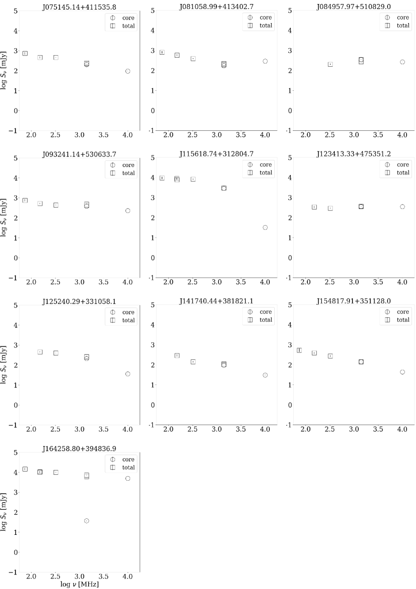
Figure 8: (a) Log-log plot of the radio flux density vs frequency. The data points include total flux densities from VLSSr, 7C, TGSS, WENSS, FIRST & NVSS. It also includes core flux densities from FIRST and the new 10 GHz measurement. Spectral slopes are not plotted for core-dominated and intermediate (Group 1 & 3) quasars as they would be affected by core variability.

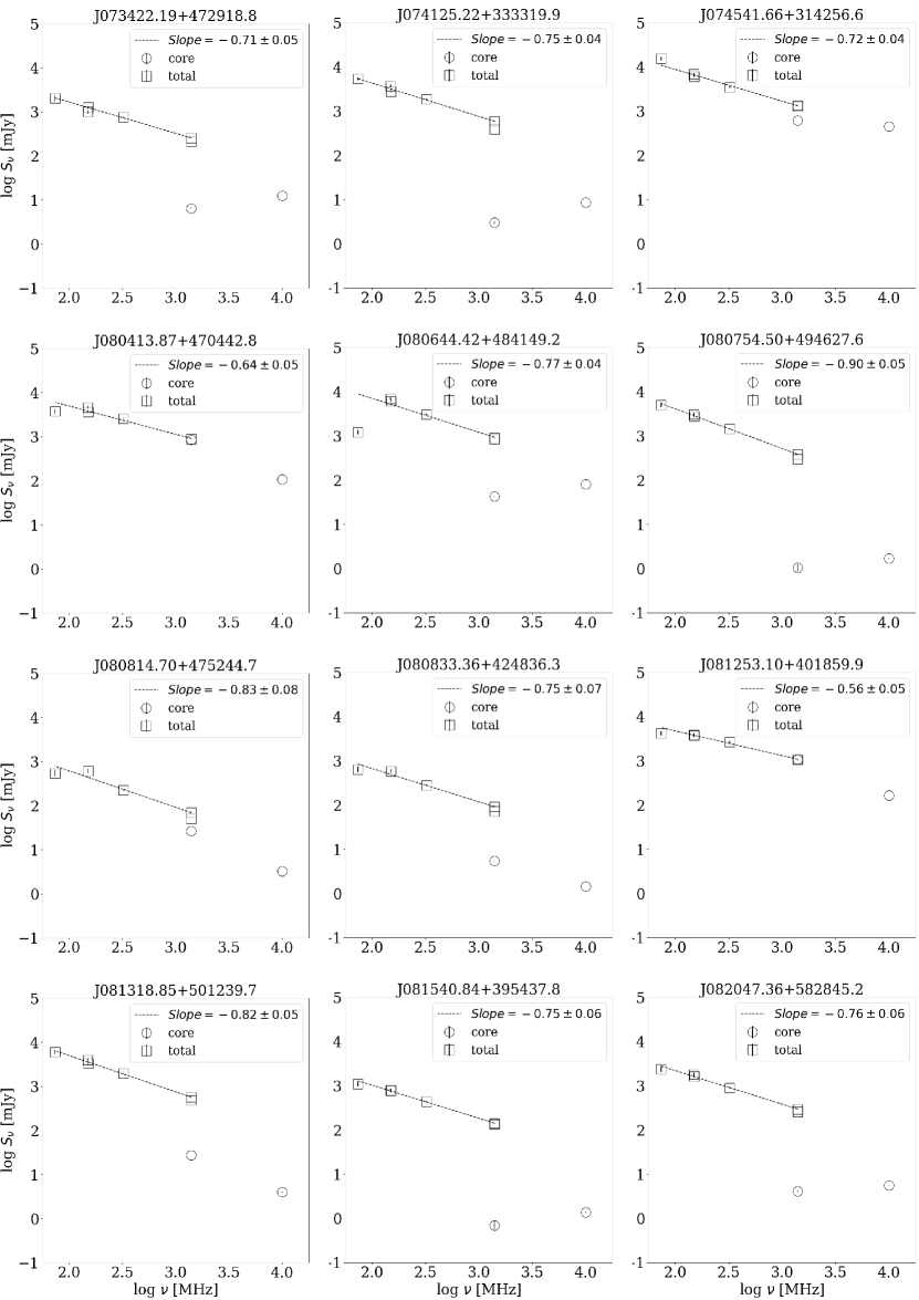
Figure 8: (b) Log-log plot of the radio flux density vs frequency. The data points include total flux densities from VLSSr, 7C, TGSS, WENSS, FIRST & NVSS. It also includes core flux densities from FIRST and the new 10 GHz measurement. Dashed line shows the spectral index of the extended emission obtained by fitting a slope to the total flux densities from VLSSr, 7C, TGSS, WENSS & NVSS. Spectral slopes are plotted for Group 2 & Group 2-flag quasars.

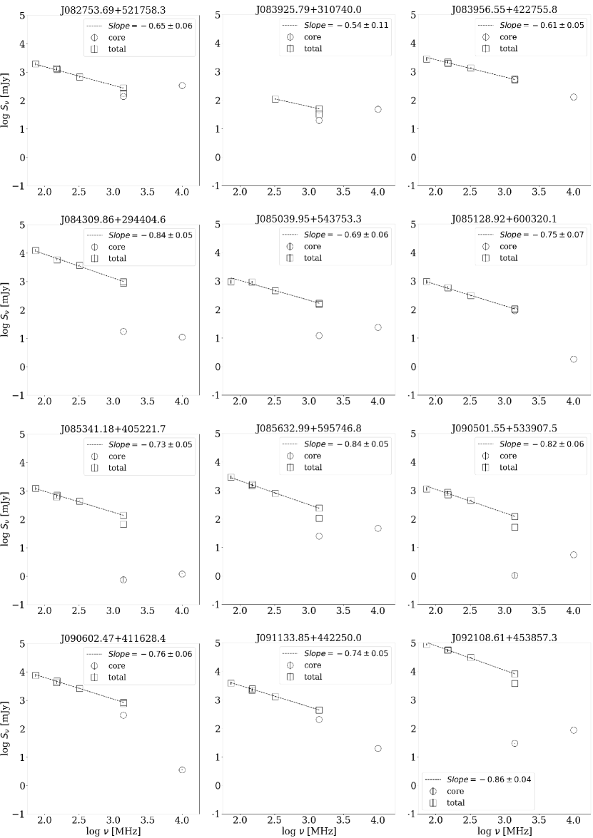
Figure 8 (b) Continued:

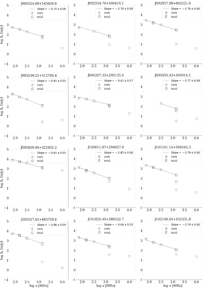
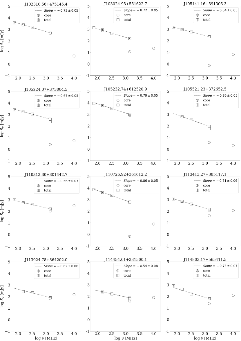
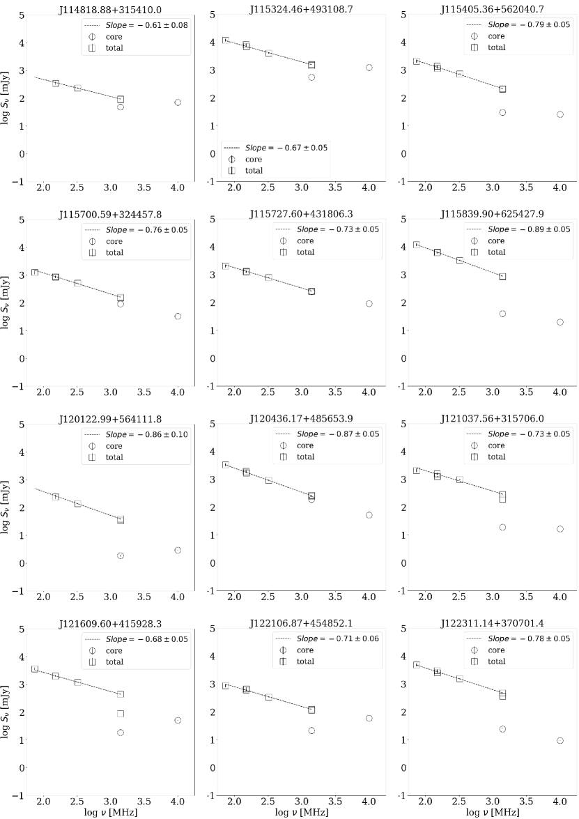
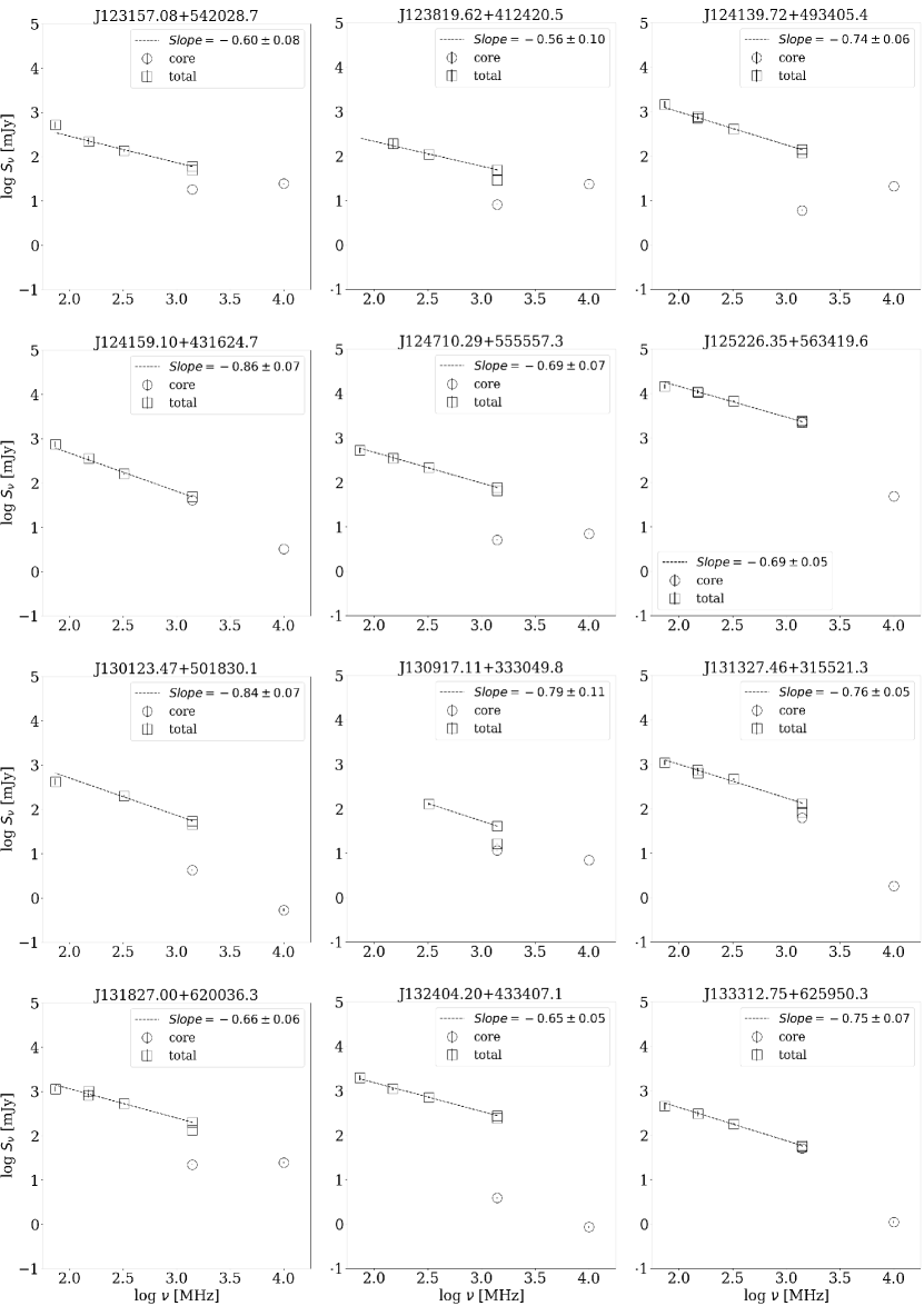
Figure 8 (b) Continued:

Figure 8 (b) Continued:

Figure 8 (b) Continued:

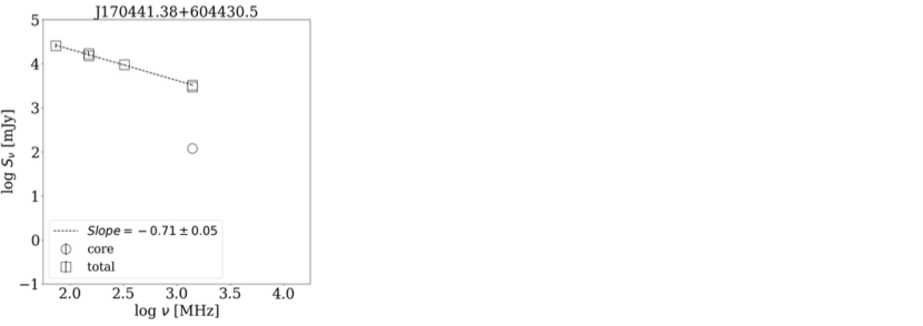
Figure 8 (b) Continued:

Figure 8 (b) Continued:

Figure 8 (b) Continued:

Figure 8 (b) Continued:

Figure 8 (b) Continued:

Appendix B Sources with resolved 10 GHz images

Table 3: RMS, mean and dynamical range of the resultant maps of VLA 10 GHz presented in this paper.

Object name	RMS	Mean	Dynamical Range
SDSS	Jy beam-1	Jy beam-1
J080413.87+470442.8	2.44E-03	1.15E-04	44.05
J085128.92+600320.1	8.66E-05	1.34E-05	21.06
J100611.67+294027.0	1.34E-04	5.62E-06	60.59
J124159.10+431624.7	1.13E-04	1.24E-05	28.89
J125226.35+563419.6	1.54E-02	2.08E-03	20.62
J164311.34+315618.4	2.61E-04	5.74E-05	13.72
J170334.99+391735.6	2.72E-05	6.08E-07	22.13

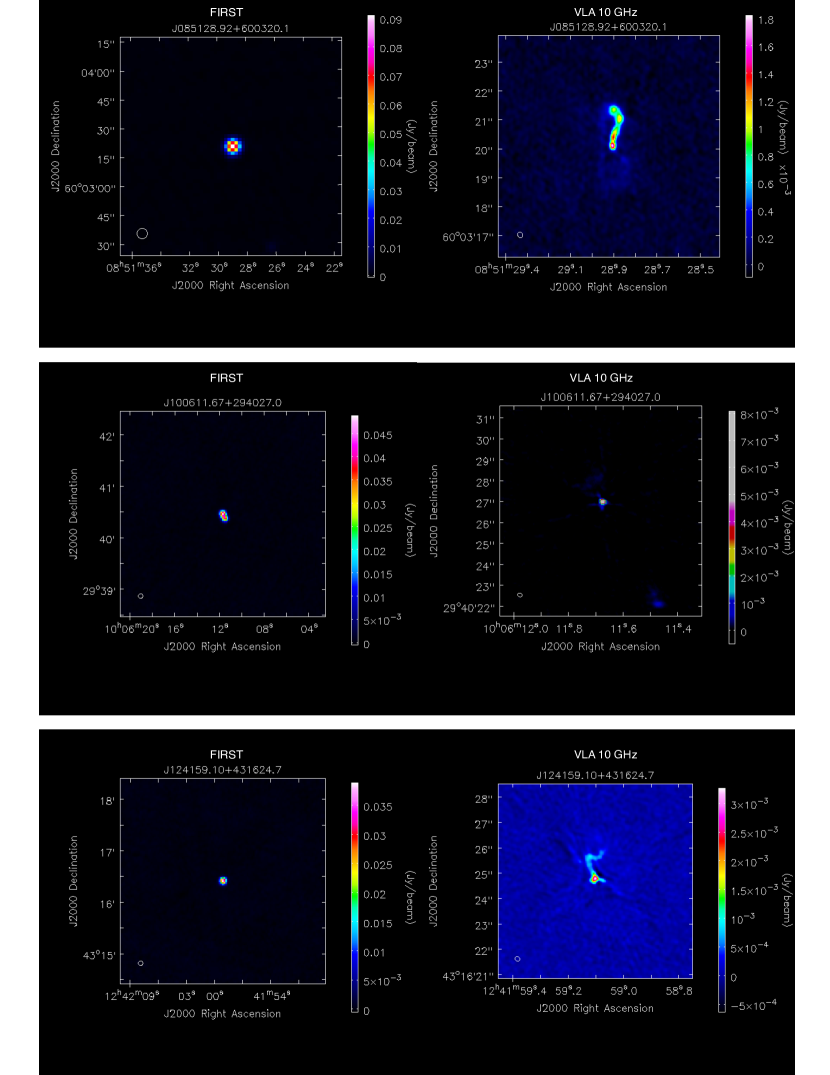
Figure 9: The FIRST image (on the left) of half a dozen targets compared to the new observation at 10 GHz (on the right). The high resolution 10 GHz images show extended structures that are unresolved at FIRST resolution.

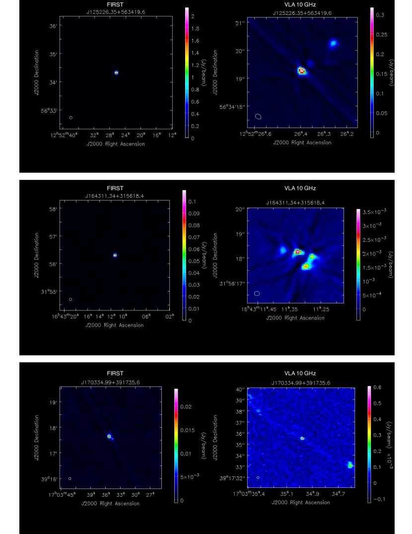
Figure 9 (Cont.):

Appendix C Additional objects

Table 4: Data for 28 additional objects observed with VLA.

Object name	Redshift	F5100	$\rm S^{core}_{10GHz}$	$\rm S^{core}_{1.4GHz}$	$\rm S_{WENSS}^{total}$	$\rm S_{TGSS}^{total}$	$\rm S_{7C}^{total}$	$\rm S_{VLSSr}^{total}$	$\rm\alpha_{ext}$	Group	log($\rm R_{1.4GHz}$)	log($\rm R_{10GHz}$)	log($\rm R_{5100,1.4GHz}$)	log($\rm R_{5100,10GHz}$)
SDSS	z		$(\rm mJy~{}beam^{-1})$	$(\rm mJy~{}beam^{-1})$	$(\rm mJy$)	$(\rm mJy$)	$(\rm mJy$)	$(\rm mJy$)
J081432.11+560956.6	0.5093	7.23$\pm$0.25	19.7$\pm$0.07	69.18$\pm$0.16	67$\pm$6	124.2$\pm$13.2	$\cdots$	$\cdots$		g3	1.08$\pm$0.053	0.53$\pm$0.053	3.04$\pm$0.03	2.50$\pm$0.03
J084925.89+564132.1	0.5882	5.71$\pm$0.27	1.02$\pm$0.02	1.42$\pm$0.15	62$\pm$7	119.5$\pm$12.1	$\cdots$	$\cdots$		g2	-0.95$\pm$0.226	-1.10$\pm$0.201	1.46$\pm$0.12	1.31$\pm$0.05

Note. — Table 4 is published in its entirety in the machine readable format. A portion is shown here for guidance regarding its form and content.

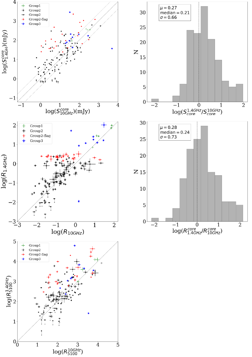
Figure 10: The left panels show scatter plots of core flux density measured at 1.4 GHz and 10 GHz and the corresponding R and $\rm R_{5100}$ measurements on log scales. The points are color coded according to the groups defined by the radio spectra of their extended emission. Points on the bottom left corner panel with downward arrows represent the objects with FIRST flux limits. The dashed lines show where the two quantities are equal. Top left: A scatter plot with the logarithm of 1.4 GHz core flux density on y-axis and the logarithm of 10 GHz core flux density on the x-axis. The dotted line represents $\rm y=x\pm 0.39$, an estimate of the $1\sigma$ scatter introduced by the core variability. Middle left: scatter plot of log R calculated from the 1.4 GHz FIRST cores on the y-axis and from the 10 GHz cores on the x-axis normalized by the extended flux densities scaled to 5 GHz rest-frame according to the groups as discussed in section 5. Bottom left: scatter plot of $\rm R_{5100}$ values calculated from the ratio of 10 GHz vs 1.4 GHz core flux densities and 5100Å flux density. The point with black open circle represent a quasar with a bad 5100 Å flux density measurement. Right: panels show the histograms of the corresponding ratio of the quantities in the x and y axis of the left panels. The dashed lines in these histograms show where the ratios are equal.

References

- Antonucci & Miller (1985) Antonucci, R. R. J., & Miller, J. S. 1985, ApJ, 297, 621, doi: 10.1086/163559
- Barthel et al. (2000) Barthel, P. D., Vestergaard, M., & Lonsdale, C. J. 2000, A&A, 354, 7
- Becker et al. (1995) Becker, R. H., White, R. L., & Helfand, D. J. 1995, ApJ, 450, 559, doi: 10.1086/176166
- Bridle et al. (1994) Bridle, A. H., Hough, D. H., Lonsdale, C. J., Burns, J. O., & Laing, R. A. 1994, AJ, 108, 766, doi: 10.1086/117112
- Briggs (1995) Briggs, D. S. 1995, New Mexico Institute of Mining Technology
- Brotherton et al. (2015) Brotherton, M. S., Singh, V., & Runnoe, J. 2015, MNRAS, 454, 3864, doi: 10.1093/mnras/stv2186
- Browne & Wright (1985) Browne, I. W. A., & Wright, A. E. 1985, MNRAS, 213, 97, doi: 10.1093/mnras/213.1.97
- Clark (1980) Clark, B. G. 1980, A&A, 89, 377
- Condon et al. (1998) Condon, J. J., Cotton, W. D., Greisen, E. W., et al. 1998, AJ, 115, 1693, doi: 10.1086/300337
- de Bruyn et al. (2000) de Bruyn, G., Miley, G., Rengelink, R., et al. 2000, VizieR Online Data Catalog, 8062
- DiPompeo et al. (2014) DiPompeo, M. A., Myers, A. D., Brotherton, M. S., Runnoe, J. C., & Green, R. F. 2014, ApJ, 787, 73, doi: 10.1088/0004-637X/787/1/73
- Dunn et al. (2006) Dunn, R. J. H., Fabian, A. C., & Sanders, J. S. 2006, MNRAS, 366, 758, doi: 10.1111/j.1365-2966.2005.09928.x
- Event Horizon Telescope Collaboration et al. (2019) Event Horizon Telescope Collaboration, Akiyama, K., Alberdi, A., et al. 2019, ApJ, 875, L1, doi: 10.3847/2041-8213/ab0ec7
- Fanti et al. (2001) Fanti, C., Pozzi, F., Dallacasa, D., et al. 2001, A&A, 369, 380, doi: 10.1051/0004-6361:20010051
- Gower et al. (1982) Gower, A. C., Gregory, P. C., Unruh, W. G., & Hutchings, J. B. 1982, ApJ, 262, 478, doi: 10.1086/160442
- Gravity Collaboration et al. (2018) Gravity Collaboration, Sturm, E., Dexter, J., et al. 2018, Nature, 563, 657, doi: 10.1038/s41586-018-0731-9
- Hales et al. (2007) Hales, S. E. G., Riley, J. M., Waldram, E. M., Warner, P. J., & Baldwin, J. E. 2007, MNRAS, 382, 1639, doi: 10.1111/j.1365-2966.2007.12392.x
- Helmboldt et al. (2007) Helmboldt, J. F., Taylor, G. B., Tremblay, S., et al. 2007, ApJ, 658, 203, doi: 10.1086/511005
- Hogg et al. (2002) Hogg, D. W., Baldry, I. K., Blanton, M. R., & Eisenstein, D. J. 2002, arXiv e-prints, astro. https://arxiv.org/abs/astro-ph/0210394
- Hovatta et al. (2014) Hovatta, T., Aller, M. F., Aller, H. D., et al. 2014, AJ, 147, 143, doi: 10.1088/0004-6256/147/6/143
- Hunstead et al. (1984) Hunstead, R. W., Murdoch, H. S., Condon, J. J., & Phillips, M. M. 1984, MNRAS, 207, 55, doi: 10.1093/mnras/207.1.55
- Intema et al. (2017) Intema, H. T., Jagannathan, P., Mooley, K. P., & Frail, D. A. 2017, A&A, 598, A78, doi: 10.1051/0004-6361/201628536
- Jackson & Browne (2013) Jackson, N., & Browne, I. W. A. 2013, MNRAS, 429, 1781, doi: 10.1093/mnras/sts468
- Jackson et al. (1989) Jackson, N., Browne, I. W. A., Murphy, D. W., & Saikia, D. J. 1989, Nature, 338, 485, doi: 10.1038/338485a0
- Kapahi & Shastri (1987) Kapahi, V. K., & Shastri, P. 1987, MNRAS, 224, 17p, doi: 10.1093/mnras/224.1.17P
- Kimball & Ivezić (2008) Kimball, A. E., & Ivezić, Ž. 2008, AJ, 136, 684, doi: 10.1088/0004-6256/136/2/684
- Kimball et al. (2011) Kimball, A. E., Ivezić, Ž., Wiita, P. J., & Schneider, D. P. 2011, AJ, 141, 182, doi: 10.1088/0004-6256/141/6/182
- Lacy et al. (2019) Lacy, M., Baum, S. A., Chandler, C. J., et al. 2019, arXiv e-prints, arXiv:1907.01981. https://arxiv.org/abs/1907.01981
- Lane et al. (2012) Lane, W. M., Cotton, W. D., Helmboldt, J. F., & Kassim, N. E. 2012, Radio Science, 47, RS0K04, doi: 10.1029/2011RS004941
- Lane et al. (2014) Lane, W. M., Cotton, W. D., van Velzen, S., et al. 2014, MNRAS, 440, 327, doi: 10.1093/mnras/stu256
- Liao & Gu (2020) Liao, M., & Gu, M. 2020, MNRAS, 491, 92, doi: 10.1093/mnras/stz2981
- Ma et al. (2019) Ma, B., Shang, Z., & Brotherton, M. S. 2019, Research in Astronomy and Astrophysics, 19, 169, doi: 10.1088/1674-4527/19/12/169
- Marin (2016) Marin, F. 2016, Monthly Notices of the Royal Astronomical Society, 460, 3679, doi: 10.1093/mnras/stw1131
- Marin & Antonucci (2016) Marin, F., & Antonucci, R. 2016, ApJ, 830, 82, doi: 10.3847/0004-637X/830/2/82
- McConnell & Ma (2013) McConnell, N. J., & Ma, C.-P. 2013, ApJ, 764, 184, doi: 10.1088/0004-637X/764/2/184
- McMullin et al. (2007) McMullin, J. P., Waters, B., Schiebel, D., Young, W., & Golap, K. 2007, in Astronomical Society of the Pacific Conference Series, Vol. 376, Astronomical Data Analysis Software and Systems XVI, ed. R. A. Shaw, F. Hill, & D. J. Bell, 127
- Nemmen & Brotherton (2010) Nemmen, R. S., & Brotherton, M. S. 2010, MNRAS, 408, 1598, doi: 10.1111/j.1365-2966.2010.17224.x
- O’Dea (1998) O’Dea, C. P. 1998, PASP, 110, 493, doi: 10.1086/316162
- Orr & Browne (1982) Orr, M. J. L., & Browne, I. W. A. 1982, MNRAS, 200, 1067, doi: 10.1093/mnras/200.4.1067
- Perley & Butler (2013) Perley, R. A., & Butler, B. J. 2013, The Astrophysical Journal Supplement Series, 204, 19, doi: 10.1088/0067-0049/204/2/19
- Rawlings & Saunders (1991) Rawlings, S., & Saunders, R. 1991, Nature, 349, 138, doi: 10.1038/349138a0
- Rengelink et al. (1997) Rengelink, R. B., Tang, Y., de Bruyn, A. G., et al. 1997, A&AS, 124, 259, doi: 10.1051/aas:1997358
- Roberts et al. (2015) Roberts, D. H., Saripalli, L., & Subrahmanyan, R. 2015, ApJ, 810, L6, doi: 10.1088/2041-8205/810/1/L6
- Runnoe & Boroson (2020) Runnoe, J., & Boroson, T. 2020, arXiv e-prints, arXiv:2004.07196. https://arxiv.org/abs/2004.07196
- Runnoe et al. (2013a) Runnoe, J. C., Brotherton, M. S., Shang, Z., Wills, B. J., & DiPompeo, M. A. 2013a, MNRAS, 429, 135, doi: 10.1093/mnras/sts322
- Runnoe et al. (2013b) Runnoe, J. C., Shang, Z., & Brotherton, M. S. 2013b, MNRAS, 435, 3251, doi: 10.1093/mnras/stt1528
- Schneider et al. (2007) Schneider, D. P., Hall, P. B., Richards, G. T., et al. 2007, AJ, 134, 102, doi: 10.1086/518474
- Schwab (1984) Schwab, F. R. 1984, AJ, 89, 1076, doi: 10.1086/113605
- Shang et al. (2011) Shang, Z., Brotherton, M. S., Wills, B. J., et al. 2011, ApJS, 196, 2, doi: 10.1088/0067-0049/196/1/2
- Van Gorkom et al. (2015) Van Gorkom, K. J., Wardle, J. F. C., Rauch, A. P., & Gobeille, D. B. 2015, MNRAS, 450, 4240, doi: 10.1093/mnras/stv912
- Verschuur et al. (1988) Verschuur, G., Kellermann, K., & Bouton, E. 1988, Galactic and extragalactic radio astronomy, Astronomy and astrophysics library (Springer-Verlag). https://books.google.com/books?id=WwIbAQAAIAAJ
- Willott et al. (1999) Willott, C. J., Rawlings, S., Blundell, K. M., & Lacy, M. 1999, MNRAS, 309, 1017, doi: 10.1046/j.1365-8711.1999.02907.x
- Wills & Brotherton (1995) Wills, B. J., & Brotherton, M. S. 1995, ApJ, 448, L81, doi: 10.1086/309614
- Wills & Browne (1986) Wills, B. J., & Browne, I. W. A. 1986, ApJ, 302, 56, doi: 10.1086/163973
- Yee & Oke (1978) Yee, H. K. C., & Oke, J. B. 1978, ApJ, 226, 753, doi: 10.1086/156657
- York et al. (2000) York, D. G., Adelman, J., Anderson, John E., J., et al. 2000, AJ, 120, 1579, doi: 10.1086/301513