DeepIntent: ImplicitIntent based Android IDS with E2E Deep Learning architecture

Abstract

The Intent in Android plays an important role in inter-process and intra-process communications. The implicit Intent that an application could accept are declared in its manifest and are amongst the easiest feature to extract from an apk. Implicit Intents could even be extracted online and in real-time. So far neither the feasibility of developing an Intrusion Detection System solely on implicit Intent has been explored, nor are any benchmarks available of a malware classifier that is based on implicit Intent alone. We demonstrate that despite Intent is implicit and well declared, it can provide very intuitive insights to distinguish malicious from non-malicious applications. We conducted exhaustive experiments with over 40 different end-to-end Deep Learning configurations of Auto-Encoders and Multi-Layer-Perceptron to create a benchmark for a malware classifier that works exclusively on implicit Intent. Using the results from the experiments we create an intrusion detection system using only the implicit Intents and end-to-end Deep Learning architecture. We obtained an area-under-curve statistic of $0.81$, and accuracy of $77.2\%$ along with false-positive-rate of $0.11$ on Drebin dataset.

I Introduction

Due to the open nature of its framework, a single Android smartphone can simultaneously run a large number of third party applications. This makes Android the most preferred mobile platform globally amongst both its potential customers and also malware developers and designers. Android uses inter-process communication so that the components could be used across processes, even those that belong to different applications. The inter-process communication mechanism is also used as a gateway to access different sensitive services in the Android framework. This communication mechanism is driven by a late run-time binding object called Intent.

Intent is a messaging object that an app can use to request an action from another app component. When the calling and serving app components are part of the same app then it is called intra-process communication; and when these components reside in different apps, it is called inter-process communication. Intent can be used for requesting actions like Starting an activity, Starting a service, Delivering a broadcast[1], etc.

Android supports two types of Intent, namely Explicit Intent and Implicit Intent. In Explicit Intent, the calling app or app component knows the app or app component which can best provide the required activity/ service. Hence the requesting app explicitly specify which application will serve the required Intent. This is indicated by supplying just the target app’s package name or a fully-qualified component class name. In Implicit Intent, the calling app or app component may not be aware of the available application that could optimally service that desired Intent. Hence the requesting app just declare a general action to perform, which allows a component from another app to service it. The Android system receives such Intent from the requesting app and finds target applications that could handle and service the requested Intent. The Android system uses the declarations made in the AndroidManifest.xml file of all installed applications to discover such potential target app. If there is only a single application available that could accept the requested implicit Intent, the Android system directly passes the associated message to that application; otherwise, it let the user choose from a list of all discovered potential applications that could serve the requested Implicit Intent.

To empower this mechanism, an application that has the required functionality to serve a requested implicit Intent (and wish to receive requests from other applications to serve the same), needs to declare such Intents in the Intent Filter of its manifest file.

Therefore a declaration of an Intent in the intent filter within an app’s manifest is useful only to inform the Android system that the specific app could accept and serve some particular implicit Intents from other requesting applications. Despite such declaration, a requested Intent would be routed to the declaring app only when such a request originates from any other app and the user manually choose this app as the preferred target from a list of competing candidate applications that could service the same Implicit Intent.

Hence, such implicit and declared Intent may not provide as expressive features for detection of potential malicious nature. Richer insights could supposedly come from analysis of API calls, permissions, op-codes or even the activities that these apps conduct while serving the received implicit Intent request. Hence, not many IDS use such implicit Intents for malware detection. To the best of our information, no IDS has been explored or developed that use implicit Intents exclusively; and no-prior art has covered the effectiveness of Malware detection using exclusively such declared, implicit, Intents. Implicit Intents could be extracted directly from an apk’s manifest (along with permissions), and hence are amongst the easiest to extract features from an apk and could even be extracted in real-time without requiring any sandbox or 3rd party services. Hence such implicit Intent could be used for developing an easy to implement independent online IDS. But, to the best of our knowledge, no benchmark exists of any IDS/ malware-classifier that exclusively use Implicit Intent.

End-to-end (E2E) Deep Learning(DL) is a type of Deep Learning where the raw inputs are converted to the desired output/predictions using all DL models and obviates manual feature engineering. E2E DL has recently become very popular in almost all advanced applications of AI. This approach has been successfully applied to many actively researched problems ranging from image classification [2, 3] to neural-machine-translation [4] to search [5] and have delivered class-leading performance. E2E DL architectures have shown good potential in the area of malware detection in Portable Executable (PE) [6, 7, 8]. But in the case of Android malware classification DL has been used more conservatively and not in E2E manner. To the best of our information, this is the first work that uses an E2E DL approach for making an Android IDS.

The major contributions of this paper are as follows:

• Exploring the richness and intuitiveness of the insights that are provided by the Implicit Intents.

• Evaluating over $40$ E2E DL configurations of Auto Encoders (AE) and Multi-Layer Perceptron based Deep Neural Networks (MLP-DNN) in a structured manner and creating performance benchmarks for malware classification that use Implicit Intent as the only features.

• Designing an easy to implement online IDS named DeepIntent that use and E2E DL implementation for both unsupervised feature engineering and supervised learning and use implicit Intents as the only features.

• Demonstrating that even with Implicit Intent alone, a very potent IDS can be developed and the resulting IDS could detect a malicious android application with an AUC of $0.81$, accuracy of $77.2\%$ along with a FPR of $0.11$.

The rest of the paper is organized as follows. Section II discusses the related work on various static features and algorithms used for Android IDS. Section III explains the experimental dataset and section IV elaborates on insights from Implicit Intents extracted from the dataset. Section V describes over $40$ configurations of different deep learning architectures that were explored for making an effective and efficient IDS. In section VI we discuss the experimental results and finally conclude the paper in section VII.

II Related Work

Lately, the practice of developing an effective and easy to implement IDS for Android applications has evolved. Besides the conventional signature-based detection, a lot of machine learning-based detection techniques have also been attempted. The two essential aspects of any machine learning-based classifier are the input features and model algorithms. Static or dynamic/behavioural analysis are used to extract input features for the IDS. Since static features are extracted without executing the apps, these could be extracted at comparatively lower-cost and are thus efficient while ensuring broad coverage in real-time for an online IDS.

Amongst the static features used for an Android IDS, (Android) permission are very popular. Au et al. developed PScout [9] to analyze permissions from different versions of Android. They discovered that despite there is little redundancy in the specification of the $75$ permissions in Androids there is up to $22\%$ redundancy in the usage of the documented APIs. Lindorfer et al. developed an online service called ANDRUBIS [10]. They found that there is a difference in the number of permissions requested by benign versus malicious apps, where benign applications request far fewer permissions on average than their malicious counterparts. Though permissions are easy to extract, unlike op-codes, they do not offer semantically rich and useful insights. Therefore where some researchers like Puerta et al. [11] and Li et al. [12] have focused exclusively on op-codes; others like Ashu et al. [13], and Idrees et al. [14] have used a combination of permissions and op-codes for making an effective malware detection system. Besides a combination of permissions and op-codes, some recent works have also explored a combination of other features with permission. For example, DroidSieve [15] combine permissions with other features like API calls, code structure, and the set of invoked components.

Recently the development of IDS using permissions with Intent has also gained traction. Wu et al. developed DroidMat, which uses permission, intent, and API Call for making a malware classifier [16]. Similarly, Arp et al. used permission, intent, API call, and network address [17]. Ali et al. developed AndroDialysis that does not use permissions, but uses both implicit and explicit Intent for making an android malware detector [18]. To the best of our knowledge, there exists no prior art which has explored making an Android IDS exclusively using implicit Intent.

In the area of model algorithms, various algorithms have been used for feature engineering and classification to develop a comprehensive Android IDS. Hemant et al. [19] focused mainly on unsupervised learning and explored different types of clustering algorithms like K-means, Aggloromative BIRCH, DBSCAN and Gaussian Mixture Models for aiding a Random Forest-based IDS classifier; whereas Ashu et al. explored similar idea with functional tree [13]. DroidMat [16] used supervised models like k-nearest-neighbour and naive-bayes for building the malware classifier. Similarly, Arp et al. [17] utilized support vector machines (SVM) for the classification of malware. Rana et al. [20] used multiple tree-based classifiers like a decision tree, random forest, gradient boosting, extremely randomized tree and random forest classifier on Android malware detection. Besides these, machine learning algorithms like Hidden Markov Model (HMM) [21], Logistic Regression, and Bayesian Networks are also popular [22] for Android malware classification.

III Dataset and Pre-Processing

In this section we discuss the malware dataset used, approach to collect and validate the complementing benign apps and the process to extract the Implicit Intents from these.

III-A Android Malware and benign applications

We have used the ‘Drebin’ dataset[17] containing $5,560$ malware samples. The dataset contains samples from more than $20$ malware families.Drebin dataset is a superset of Android Malware Genome Project[23] which was proposed by Zhou et al. and contain more than $1,200$ malware samples. We downloaded more than $7,500$ Android applications from Google Play store. We used the online service of VirusTotal for validating the downloaded application as benign. An Android app was labelled as benign if all the antivirus subscribed by VirusTotal label it as non-malicious. We performed the exercise for all the downloaded applications and discarded the malicious ones. Finally, the benign dataset consists of $5,721$ benign Android apps.

III-B Extraction of Intents

APKTOOL, a $3^{rd}$ party reverse engineering tool, was used to disassemble the android applications (.apk extension). It can decode an Android application into source files (including resources.arsc, classes.dex, XMLs etc.) and can also be used to recompile the application. Each application contains AndroidManifest(.xml) file which describes essential information like App activities, services, broadcast receivers etc. and are activated by intents. We extracted all the ($273$) Intent used by an application using a custom parser.

IV Analysis of Implicit Intent

Since the malware and benign applications in the data set were mostly balanced, the Intent counts were directly analyzed without further normalization. Top $10$ Intents on the basis of total Intent count that are found in malicious applications (table I) and non-malicious samples (table II) are tabulated. It was found that some Intents like BOOT_COMPLETED, ACTION_POWER_CONNECTED, INPUT_METHOD_CHANGED, UMS_CONNECTED etc. were comparatively more frequent in malicious apps than in non-malicious apps. For non-malicious apps, the most frequent unique Intents were BROWSABLE, SEARCH, PICK, INFO etc. This difference between frequent Intents between the two classes of apps is a good indicator of the malicious modus-operandi of malicious applications.

TABLE I: Top-10 Intent used in malicious apps

Type	Name	Count	Rank
action	MAIN	7543	1
category	LAUNCHER	6107	2
action	BOOT COMPLETED	4138	3
category	HOME	1881	4
category	DEFAULT	1524	5
action	USER PRESENT	607	6
action	VIEW	496	7
action	ACTION POWER CONNECTED	295	8
action	INPUT METHOD CHANGED	293	9
category	SAMPLE CODE	249	10

TABLE II: Top-10 Intent used in non-malicious apps

Type	Name	Count	Rank
action	MAIN	7388	1
category	DEFAULT	6181	2
category	LAUNCHER	6061	3
action	VIEW	2281	4
category	BROWSABLE	1486	5
action	BOOT COMPLETED	1097	6
action	PACKAGE ADDED	385	7
action	SEARCH	325	8
action	SEND	276	9
action	USER PRESENT	270	10

To explore this dissimilarity more objectively the difference in frequency of each Intent ($I_{x}$) was computed between the malicious($\mathcal{N}^{Mal}$) and non-malicious ($\mathcal{N}^{NonMal}$) applications and the vice-versa. The obtained difference was then normalized ($\mathbb{N(\mathcal{D})}_{I_{x}}$) by the average frequency of the specific Intent across both malicious and non-malicious apps as shown in equation 1. Top 10 Intents by the average normalized difference between malicious over non-malicious ($\mathbb{N(\mathcal{D})}^{Mal}$) are shown in table III. The difference between the frequency of some Intents like the DATA_REMOVED, GTALK_CONNECTED, INPUT_METHOD_CHANGED etc was twice as much as the average frequency in the entire dataset. Intuitively understanding, this suggests that at least some malicious apps are more likely (than their non-malicious counterparts) to be dependant on the internet connection to accomplish their malicious actions. Also, some malicious apps may be engaged in malicious activities involving deletion of data of communication via installed communication apps.

$$\mathbb{N(\mathcal{D})}^{Mal}_{I_{x}}=\frac{2*(\mathcal{N}^{Mal}_{I_{x}}-\mathcal{N}^{NonMal}_{I_{x}})}{\mathcal{N}^{Mal}_{I_{x}}+\mathcal{N}^{NonMal}_{I_{x}}}$$ (1)

TABLE III: Top-10 Intent by difference between average presence in Malicious vs. Non-Malicious ones

Type	Name	Count	Rank
extra	DATA REMOVED	2	1
action	GTALK CONNECTED	2	1
action	INPUT METHOD CHANGED	2	1
action	UMS DISCONNECTED	2	1
action	UMS CONNECTED	2	1
category	HOME	1.61	6
action	BATTERY OKAY	1.61	6
category	SAMPLE CODE	1.57	8
action	BATTERY LOW	1.39	9
action	MEDIA CHECKING	1.33	10

V Experimental Setup & Configurations

Recently E2E DL architectures containing Stacked Auto Encoders (SAE) and MLP-DNN have shown maturity [24], and these have demonstrated significant progress in the malware detection [8]. Therefore in this section, we experiment with similar E2E DL configurations, including SAE/AE and MLP-DNN.

V-A Finding the best AE configuration

SAE are type of AEs that are used to generate a lower dimension representation of original data while maintaining the non-linearity amongst the input features. The input dataset contains $273$ sparse features, many of them are NULL in many applications. Such input is not optimal to be used for supervised learning. By using SAE we reduce the number of features; convert them to dense representations from sparse; and preserve the expressive non-linearity in the relationship of the features. Since the performance of MLP configurations are dependant upon the embeddings received from upstream AE, therefore we will first optimize the AE configuration.

The validation-loss of the AE network and the AUC (Area Under Curve) of a downstream standardized MLP network were used as the performance criterion to appraise the different AE configurations.

In the first stage, we optimize No. of hidden layers, and No. of neurons in each of hidden layers and size of embedding layer for the SAE. Since these three hyper-parameters are inter-dependant, thus they cannot be evaluated in isolation. Hence several experiments with a different combination of these is multiple iterations were required while eliminating redundant configurations after each iteration. In the first iteration, we started evaluating different networks with a single hidden layer of varying hidden layer size and embedding dimension.

Table IV shows the AE configurations with single hidden layer of different sizes varying from $32$ neurons to $256$ neurons that were evaluated. As there were only $273$ unique Intents, therefore configurations involving layer size above $256$ neurons was not conducted. Similarly, as the embedding size was kept constant at $32$, therefore any hidden layer size less than $32$ neurons were not evaluated. The hidden layer size that demonstrated comparable performance with the least number of neurons was fixed as the upper cap for evaluating any configuration with more than one hidden layer in other iterations.

TABLE IV: AE: Single Hidden Layer Configurations

Conf. ID	Hidden Layer Size	Embedding Dimension	AE Val. Loss	MLP AUC
1	[256]	256	0.016	0.79
2	[256]	128	0.017	0.50
3	[256]	64	0.017	0.79
4	[256]	32	0.018	0.79
5	[128]	128	0.017	0.79
6	[128]	64	0.018	0.79
7	[128]	32	0.018	0.79
8	[64]	64	0.018	0.79
9	[64]	32	0.018	0.79
10	[32]	32	0.018	0.50
11	[32]	16	0.019	0.78

Interestingly, during the first stage, some configurations demonstrated a sudden drop in performance; and configurations that had just a higher and just lower No. of neurons both had better performance. To ensure that this phenomenon was not just because of some trivial random No. initialization, these configurations were re-evaluated with a different random No. seed; but their performance did not change much, and hence these configurations along with some other were dropped in the next iteration.

In the second iteration, AE configurations with up to two hidden layers were evaluated. The sub-optimal performance of a DL network on a training dataset could be because of data complexity or non-linearity or both. Since the requirement of more than one hidden layer over the size of a hidden layer is more indicative of non-linearity, so layer sizes above $128$ neurons were not evaluated. As shown in table V, in this iteration we evaluated two-hidden-layer configurations where the size of the first hidden layer could range between $128\geq AE_{H1}\geq 32$ and the size of the second hidden layer could range between $AE_{H1}\geq AE_{H2}\geq 32$. Since in SAE the purpose is to compress the data dimension cardinality gradually, hence above constraint is required.

TABLE V: AE: Two-Hidden-Layer Configurations

Conf. ID	Hidden Layer Size	Embedding Dimension	AE Val. Loss	MLP AUC
14	[128, 128]	32	0.017	0.5
15	[128, 64]	32	0.017	0.79
16	[128, 32]	32	0.017	0.5
17	[64, 64]	32	0.017	0.5
18	[64, 32]	32	0.017	0.5
19	[32, 32]	32	0.017	0.5

In the $3^{rd}$ iteration of AE configuration optimization, we evaluated multiple configurations with three hidden layers of varying sizes. The upper limit for the No. of layers in the first hidden layer the constraints for the same in any subsequent hidden layers were kept the same as in the $2^{nd}$ iteration. Table VI shows the various configurations of AE evaluated in the this iteration. Since none of these configurations performed as well as some other configurations with only two hidden layers as evaluated in earlier iteration, therefore configurations with more than three hidden layers were not evaluated.

TABLE VI: AE: Three-Hidden-Layer Configurations

Conf. ID	Hidden Layer Size	Embedding Dimension	AE Val. Loss	MLP AUC
20	[128, 64, 64]	32	0.017	0.5
21	128, 64, 32]	32	0.017	0.77
22	[128, 32, 32]	32	0.017	0.5

V-B Finding the best MLP DNN configuration

From the analysis of the experiments conducted in section V-A, we determine the optimal AE configuration. Using the discovered optimal AE configuration we conducted multiple experiments to select an optimal configuration of the MLP DNN as well. The criterion for evaluating MLP DNN configuration we use the AUC statistic, along with the accuracy scored on the validation data. The validation accuracy is computed when the class as derived from the class probabilities using a threshold of $0.5$ for distinguishing between the two classes.

In the next stage, we conduct experiments with different numbers of hidden layers and varying sizes of each of these hidden layers for the MLP-DNN network. We have used similar constraints and shortlisting criteria as we did in the case of AE. We evaluated different MLP DNN configurations with $1$ to $6$ No. of hidden layers and with $32$ to $256$ No. of neurons in the hidden layers. Using the shortlisting criterion as indicated earlier, we were able to obviate evaluation of many configurations that were less likely to produce better results as compared to similar configurations that also has fewer number of hidden layers. The reduced number of experiments that were mandated as per the shortlisting subsequent experimentation criterion are as indicated in table VII.

TABLE VII: MLP: Experiments for finding the best number and size of hidden layers

Conf. ID	MLP Hidden Layer Size	MLP AUC	Accuracy (Th=0.5)	FPR (Th=0.5)	Best Accuracy	FPR @ Best Accuracy	Accuracy @ Best F1	FPR @ Best F1
23	[256]	0.773	0.738	0.131	0.741	0.116	0.735	0.181
24	[128]	0.772	0.737	0.133	0.739	0.115	0.733	0.185
25	[64]	0.775	0.737	0.133	0.74	0.117	0.737	0.172
26	[32]	0.763	0.736	0.151	0.74	0.152	0.74	0.152
27	[32, 32]	0.778	0.736	0.137	0.74	0.164	0.734	0.19
28	[64, 64]	0.777	0.74	0.152	0.745	0.138	0.744	0.158
29	[128, 128]	0.781	0.744	0.141	0.746	0.151	0.746	0.151
30	[256, 256]	0.775	0.743	0.151	0.744	0.15	0.744	0.153
31	[128, 128, 128]	0.788	0.748	0.112	0.752	0.133	0.751	0.144
32	[64, 64, 64]	0.788	0.744	0.14	0.752	0.111	0.746	0.162
33	[128, 128, 128, 128]	0.501	0.514	0	0.514	0	0.486	0.999
34	[64, 64, 64, 64]	0.792	0.752	0.111	0.758	0.117	0.757	0.129
35	[128, 128, 64, 64]	0.788	0.743	0.116	0.751	0.136	0.749	0.15
36	[64, 64, 64, 64, 64]	0.788	0.74	0.126	0.75	0.137	0.745	0.161
37	[64, 64, 64, 64, 64, 64]	0.5	0.514	0	0.514	0	0.486	1

Next explored the effect of increasing the number of epochs for training. As shown in table VIII, we increased the number of epochs from $100$ (default in all previous experiments) to $1000$. Performance of configurations with more than $1000$ epochs were not evaluated as the training accuracy and loss plots obtained from the above configurations demonstrated convergence.

TABLE VIII: MLP: Effect of increasing the number of Epochs

Conf. ID	MLP Hidden Layer Size	MLP Epochs	MLP AUC	Accuracy (Th=0.5)	FPR (Th=0.5)
34	[64, 64, 64, 64]	100	0.792	0.737	0.111
38	[64, 64, 64, 64]	1000	0.802	0.738	0.101

The optimizer algorithm plays a significant role in determining both the effectiveness (as determined by performance indicators) and the efficiency of training (as indicated from the computational time). We experimented with some of the popular optimizer algorithms in DL [24] next. The default optimizer algorithm used so far was adadelta. Besides, we also experimented with the adam and rmsprop optimizers keeping other parameters same as indicated in table IX.

TABLE IX: MLP: Effect of change of Optimizer algorithm

Conf. ID	MLP Hidden Layer Size	MLP Ep- ochs	MLP Opti- mizer	MLP AUC	Acc (Th =0.5)	FPR (Th =0.5)
38	[64, 64, 64, 64]	1000	adadelta	0.802	0.768	0.101
39	[64, 64, 64, 64]	1000	adam	0.806	0.764	0.118
40	[64, 64, 64, 64]	1000	rmsprop	0.814	0.772	0.11

Another hyper-parameter closely associated with both effectiveness and efficiency is the batch-size. The default batch size used until stage $6$ was $1024$. Hence for $\sim 7700$ training records ($~{}11000\times 0.7$ training split), we made around 8 steps of training passes in each epoch. In the next iteration we experimented with different batch-sizes as shown in table X. The choice of the optimizer algorithm, along with the optimizer‘s associated hyper-parameters, like learning-rate ($\eta$) has a role to play in determining the optimal batch-size. Hence we had first finalized on the optimizer choices earlier before evaluating the different batch-sizes in this iteration.

TABLE X: MLP: Effect of change of Batch Size

Conf. ID	MLP Hidden Layer Size	MLP Batch Size	MLP Opti- mizer	MLP AUC	Acc (Th =0.5)	FPR (Th =0.5)
40	[64,64,64,64]	1024	rmsprop	0.814	0.772	0.11
41	[64,64,64,64]	2048	rmsprop	0.803	0.764	0.107
42	[64,64,64,64]	512	rmsprop	0.794	0.755	0.136

VI Results & Discussion

In section V-B we cover the experiment with multiple configurations of MLP DNN. The criteria for evaluating MLP DNN are the AUC statistic and the accuracy obtained on validation data (at prediction probability cut-off of 0.5). As shown in table VII and XI we also compute the validation accuracy and FPR using different cut-off thresholds of prediction probabilities, viz.

• the threshold cut-off of 0.5 (default for comparison),

• the threshold that gives the best accuracy (and associated FPR) even at a compromise of FPR,

• and third an accuracy and associated FPR that provides the best balance between the precision and recall as determined by the ‘F1 measure’.

We found that the MLP DNN with $4$ hidden layers, each with $64$ units, when trained with a batch-size of $1024$ records over $1000$ epochs using the ‘rmsprop’ optimizer, gave the best results. It produced an AUC statistic of $0.814$ with an accuracy of $77.2\%$ and an FPR of $0.11$ on the validation data. This configuration is indicated by Conf. ID 40, and its details are shown in table XI. The ROC plot obtained at the different threshold for prediction probability cut-offs for this configuration are shown in figure 1.

An interesting observation regarding this (best) configuration is that all the three performance milestones converge for this configuration. That is we obtain the best accuracy and also the best F1 measure (balance between precision and recall) and the default prediction probability cut-off of $0.5$.

TABLE XI: AE + MLP: Best E2E Configuration (Conf. ID 40)

Conf. ID 40
Parameter	Value	Parameter	Value
AE Hidden Lyrs.	[128,64]	MLP Hidden Lyrs.	[64,64,64,64]
AE Embedding Lyr.	32	MLP Optimizer	rmsprop
AE Batch Size	1024	MLP Batch Size	1024
AE Epochs	1000	MLP Epochs	1000
AE Val. Loss	0.006	MLP AUC	0.814
Accuracy (Th=0.5)	0.772	FPR (Th=0.5)	0.11
BestAccuracy	0.772	FPR @ BestAccuracy	0.11
Accuracy @ BestF1	0.772	FPR @ BestF1	0.11

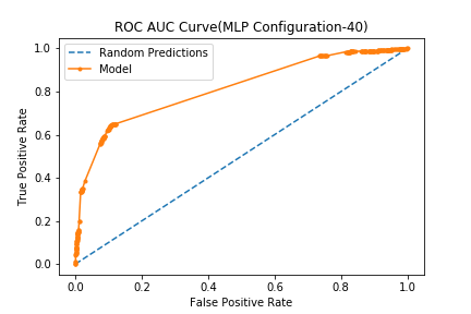
Figure 1: ROC Plot: MLP Conf. ID 40

VII Conclusion

Even amongst all static features available for Android malware analysis, Implicit Intents are the easiest to extract. In this paper we demonstrate that besides being easy to extract, these Intent are also quite intuitive to analyze descriptively. The results in section VI also proves that a potent Android IDS could also be created using Implicit Intent alone. In section V we experimented with over $40$ E2E DL configurations and established a performance benchmark for a malware classifier that uses Implicit Intent as the only features. The benchmark performance had an AUC of $0.814$, along with and accuracy of $77.2\%$ and an FPR of $0.11$.

References

[1]
AndroidDeveloperGuide, “Intents and intent filters,
https://developer.android.com/guide/components/intents-filters,” Accessed
April 8, 2020.
[2]
A. Krizhevsky, I. Sutskever, and G. E. Hinton, “Imagenet classification with
deep convolutional neural networks,” in NIPS, ser. 2012. Curran Associates Inc., 2012, p. 1097–1105.
[3]
R. Socher, B. Huval, B. Bath, C. D. Manning, and A. Y. Ng,
“Convolutional-recursive deep learning for 3d object classification,” in
Advances in neural information processing systems, 2012, pp. 656–664.
[4]
D. Bahdanau, K. Cho, and Y. Bengio, “Neural machine translation by jointly
learning to align and translate,” 2014.
[5]
D. Amodei et al., “Deep speech 2: End-to-end speech recognition in english and
mandarin,” 2015.
[6]
E. Raff, J. Barker, J. Sylvester, R. Brandon, B. Catanzaro, and C. Nicholas,
“Malware detection by eating a whole exe,” in AAAI, 2017.
[7]
M. Sewak, S. K. Sahay, and H. Rathore, “Comparison of deep learning and
the classical machine learning algorithm for the malware detection,” in
SNPD, 2018, pp. 293–296.
[8]
M. Sewak et al., “An investigation of a deep learning based malware detection
system,” in ARES, 2018, pp. 1–5.
[9]
K. Wain Yee Au et al., “Pscout: Analyzing the android permission
specification,” in ACM CCS. ACM, 2012, p. 217–228.
[10]
M. Lindorfer et al., “Andrubis – 1,000,000 apps later: A view on current
android malware behaviors,” in BADGERS, 2014, pp. 3–17.
[11]
J. Gaviria de la Puerta and B. Sanz, “Using Dalvik opcodes for malware
detection on android,” Logic Journal of the IGPL, vol. 25, no. 6,
pp. 938–948, 2017.
[12]
J. Li et al., “Significant permission identification for
machine-learning-based android malware detection,” IEEE Transactions
on Industrial Informatics, vol. 14, no. 7, pp. 3216–3225, 2018.
[13]
A. Sharma and S. K. Sahay, “An investigation of the classifiers to detect
android malicious apps,” in Information and Communication
Technology. Springer, 2018, pp.
207–217.
[14]
F. Idrees et al., “Investigating the android intents and permissions for
malware detection,” in WiMob, 2014, pp. 354–358.
[15]
G. Suarez-Tangil et al., “Droidsieve: Fast and accurate classification of
obfuscated android malware,” in CODASPY, ser. 2017. ACM, 2017, p. 309–320.
[16]
D.-J. Wu, C.-H. Mao, T.-E. Wei, H.-M. Lee, and K.-P. Wu, “Droidmat: Android
malware detection through manifest and api calls tracing,” Asia Joint
Conference on Information Security, pp. 62–69, 2012.
[17]
H. Arp et al., Daniel, K. Rieck, and C. Siemens, “Drebin: Effective and
explainable detection of android malware in your pocket,” in NDSS,
vol. 14, 2014, pp. 23–26.
[18]
A. Feizollah et al., “Androdialysis: Analysis of android intent effectiveness
in malware detection,” Computers and Security, pp. 121–134, 2017.
[19]
H. Rathore, S. K. Sahay, P. Chaturvedi, and M. Sewak, “Android malicious
application classification using clustering,” in ISDA. Springer, 2018, pp. 659–667.
[20]
M. Rana et al., “Evaluation of tree based machine learning classifiers for
android malware detection,” in Computational Collective
Intelligence. Springer, 2018, pp.
377–385.
[21]
L. Xie, X. Zhang, J.-P. Seifert, and S. Zhu, “Pbmds: A behavior-based malware
detection system for cellphone devices,” 03 2010, pp. 37–48.
[22]
A. Shabtai et al., “Andromaly: a behavioral malware detection framework for
android devices,” vol. 38, 2012, p. 161–190.
[23]
Y. Zhou and X. Jiang, “Dissecting android malware: Characterization and
evolution,” in IEEE S&P. IEEE, 2012, pp. 95–109.
[24]
M. Sewak, S. K. Sahay, and H. Rathore, “An overview of deep learning
architecture of deep neural networks and autoencoders,” Journal of
Computational and Theoretical Nanoscience, vol. 17, no. 1, pp. 182–188,
2020.