Revisiting QCD corrections to the forward-backward charge asymmetry of heavy quarks in electron-positron collisions at the Z pole: really a problem?

Abstract

We review in some detail the QCD corrections to the measurement of the forward-backward charge asymmetry of heavy quarks in the $\mathrm{e^{+}e^{-}\rightarrow Q\overline{Q}(g)}$ process at the Z pole. We show that the size of these corrections can be reduced by an order of magnitude by using simple cuts on jet acollinearity. Such a reduction is expected to lead to systematic uncertainties at the $\Delta\mathrm{A_{FB}^{0,Q}}\approx 10^{-4}$ level, opening up the path to high precision electroweak measurements with heavy flavors at future high luminosity $\mathrm{e^{+}e^{-}}$ colliders like the FCC-ee.

1 Introduction

The forward-backward asymmetry of b quarks at the Z pole, ${A_{FB}^{0,b}}$, is the electroweak observable that currently presents the largest deviation with respect to standard model expectations lephf-05 (almost a $3\sigma$ pull). Many new-physics models have been proposed to explain this discrepancy, all of them requiring a drastic enhancement of the right-handed coupling of the b quark to the Z boson Djouadi:2006rk . A significantly improved measurement at the FCC-ee could thus become a clean signal of physics beyond the standard model, provided that the deviation in the central value stays. While the world average measurement is still dominated by statistical uncertainties ($\Delta{A_{FB}^{0,b}}=0.0016$), it is also affected by non-negligible systematic uncertainties ($\Delta{A_{FB}^{0,b}}(\textrm{syst.})=0.0007$).

Legacy studies of the forward-backward asymmetry of heavy quarks (bottom, charm) in $\mathrm{e^{+}e^{-}}$ collisions at the Z pole lephf-05 ; ep-98 revealed that QCD corrections were the largest source of correlated systematic uncertainty in the combined LEP measurement. Even if some recent studies have quantified that those uncertainties are substantially reduced when the latest parton shower tunes are used Enterria , they are still expected to constitute a dominant and irreducible source of uncertainty for high-statistics measurements at future $\mathrm{e^{+}e^{-}}$ colliders. There have been some attempts to reduce the size of these uncertainties, which have a theoretical origin, through changes in the experimental analysis. For instance, in measurements employing lepton tagging, the size of the QCD corrections can be reduced by a factor of two or so by preferentially selecting events with large lepton momentum ep-98 .

The QCD corrections to the forward-backward asymmetry in ${\mathrm{e^{+}e^{-}}\to Q\overline{Q}(g)}$ were studied by many authors at the time of LEP/SLC measurements Jersak:1981sp ; Djouadi:1989uk ; Arbuzov:1991pr ; Djouadi:1994wt ; Altarelli:1992fs ; Stav:1994se , and revisited later, with a strong focus on the size of higher order contributions, in References Ravindran:1998jw ; Catani:1999nf ; Weinzierl:2006yt ; Bernreuther:2016ccf . Throughout the Note, we assume that the direction of heavy quark jet ${Q}$ is the reference for the asymmetry measurement, and not the thrust direction (which was the usual choice in LEP measurements).

In this Note we revisit this issue and explore possible approaches to perform a measurement at future colliders with systematic uncertainties at the $\Delta{A_{FB}}\approx 10^{-4}$ level. We first have a closer look to the existing calculations of the QCD corrections, showing that one can approximate them with sufficient precision using rather simple expressions. Some relevant features, which passed almost unnoticed until now, lead us to suggest an experimental approach using tighter cuts in jet acollinearity than usual. This new strategy should bring a significant reduction in the size of QCD corrections. We test the new approach using fast simulations of the IDEA detector at the future FCCee collider FCC-ee . Other potential sources of systematic uncertainty, both of theoretical and experimental origin, are also addressed in the study.

2 QCD corrections at order $\mathcal{O}({\alpha_{s}})$: massless quark limit

The explicit expressions for the QCD corrections at first order in ${\alpha_{s}}$ can be found for instance in References Jersak:1981sp ; Djouadi:1994wt . An important feature, not sufficiently emphasized at the time in theoretical papers, is that virtual QCD corrections to ${A_{FB}}$ vanish in the massless quark limit. The absence of soft-collinear divergences in the calculation implies that the total estimate of QCD corrections is reduced to the quantification of the corrections to the ${Q\overline{Q}g}$ process, with one real gluon emitted. These hard corrections stay finite even when approaching the configuration where the gluon is collinear with one of the quarks or, equivalently, where the two quark jets are back-to-back.

By convention, the QCD corrections are expressed in terms of the factor $C(m_{Q})$:

$$\frac{\Delta{A_{FB}}}{{A_{FB}}} = -\frac{{\alpha_{s}}}{\pi}~{}C(m_{Q})\;.$$ (1)

In the massless limit it is easy to prove that the $C$ factor is obtained by a simple integration Jersak:1981sp ; Djouadi:1994wt :

$$C(0) = \frac{4}{3}~{}\int_{{x_{min}}}^{{x_{max}}}dx\int_{{\overline{x}_{min}}(x)}^{{\overline{x}_{max}}(x)}d{\overline{x}}~{}\left(\frac{{\overline{x}}}{x}\right)\;,$$ (2)

where $x$ and ${\overline{x}}$ are the reduced energies of the heavy quarks in the $\mathrm{e^{+}e^{-}}\to{Q\overline{Q}(g)}$ process: $x\equiv 2E_{Q}/{\sqrt{s}}$, ${\overline{x}}\equiv 2E_{\overline{Q}}/{\sqrt{s}}$. When integrated over the full available phase space, the limits of the integral are: ${\overline{x}_{min}}(x)=1-x,{\overline{x}_{max}}(x)=1,{x_{min}}=0,{x_{max}}=1$, leading to the known result:

$$C(0,\text{full phase space}) = \frac{4}{3}~{}\int_{0}^{1}dx\int_{1-x}^{1}d{\overline{x}}~{}\left(\frac{{\overline{x}}}{x}\right)=1\;.$$ (3)

In this context, it is possible to apply cuts on observables that depend on $x$ and ${\overline{x}}$. One example is the acollinearity $\xi$ between quark and antiquark directions Djouadi:1994wt :

$$\cos\xi(x,{\overline{x}}) = 1-2~{}\frac{(1-x)~{}(1-{\overline{x}})}{x~{}{\overline{x}}}$$

$$\Downarrow$$

$${\displaystyle\sin^{2}(\xi(x,{\overline{x}})/2)} = \frac{(1-x)~{}(1-{\overline{x}})}{x~{}{\overline{x}}}\;.$$ (5)

The limits for an acollinearity cut $\xi<\xi_{0}$ are ${\overline{x}_{min}}(x)=(1-x)/(1-x+\epsilon_{0}x)$, ${\overline{x}_{max}}(x)=1$, ${x_{min}}=0,{x_{max}}=1$, where we define: $\epsilon_{0}\equiv\sin^{2}(\xi_{0}/2)$. With this we obtain the more general expression:

$$\epsilon_{0} \equiv \sin^{2}(\xi_{0}/2)$$

$$\Downarrow$$

$$C(0,\xi<\xi_{0}) = \int_{0}^{1}dx\int_{\frac{1-x}{1-x+\epsilon_{0}x}}^{1}d{\overline{x}}~{}\left(\frac{4{\overline{x}}}{3x}\right)={\displaystyle\frac{-2\epsilon_{0}\left[(2-\epsilon_{0})(\log\epsilon_{0})+1-\epsilon_{0}\right]}{3(1-\epsilon_{0})^{2}}}\;.$$ (7)

From Equation 7 we derive the results listed in Table 1. They show that the correction factor can be significantly reduced with the use of acollinearity cuts. For instance, for $\xi_{0}=0.3$, which is still larger than the typical angular resolution of experimental jets, C(0) is reduced by one order of magnitude.

$\xi_{0}$ cut	$C(0,\xi<\xi_{0})$
No cut	$1.000$
$1.50$	$0.693$
$1.00$	$0.473$
$0.50$	$0.207$
$0.30$	$0.102$
$0.20$	$0.055$
$0.10$	$0.018$
$0.05$	$0.006$

Table 1: QCD correction factor $C$ in the massless quark limit ($m_{Q}=0$), for different acollinearity cuts $\xi<\xi_{0}$ between the two quarks in the $\mathrm{e^{+}e^{-}}\to{Q\overline{Q}(g)}$ process.

3 QCD corrections at order $\mathcal{O}({\alpha_{s}})$: the massive case ($m_{Q}\neq 0$)

In the massive case, even at order ${\alpha_{s}}$, virtual QCD corrections to the asymmetry are not zero, and soft, virtual and hard corrections must be added together in order to obtain finite results. The first order corrections can be expanded in powers of the small parameter $\mu\equiv 2~{}m_{Q}/{\sqrt{s}}$ Stav:1994se ($\mu\approx 0.1$ at the Z pole for b-quarks). Fortunately, the explicitly divergent terms lead to corrections of order $\mu^{2}\approx 0.01$, and the leading corrections can be calculated to a good approximation by just updating to the massive case the limits of integration in Equation 2. This key detail at order ${\alpha_{s}}$ was already noticed by the authors of Reference Altarelli:1992fs . Accordingly, we can obtain an approximation to $C(m_{Q})$ at the percent level from rather simple numerical integrations. This precision is sufficient for our purposes. For instance, let us note that the ${\cal O}({\alpha_{s}}^{2}$) corrections to the asymmetry Altarelli:1992fs ; Ravindran:1998jw ; Catani:1999nf ; Weinzierl:2006yt ; Bernreuther:2016ccf are at least one order of magnitude larger than the uncertainties due to the approximation employed here.

In the massive case the acollinearity angle between the two quarks in the ${Q\overline{Q}g}$ final state has the following dependence on $x,{\overline{x}}$ and $\mu$ Djouadi:1994wt :

$$\cos\xi(x,{\overline{x}},\mu) = \frac{x{\overline{x}}-\mu^{2}-2~{}(1-x)~{}(1-{\overline{x}})}{\sqrt{x^{2}-\mu^{2}}~{}\sqrt{{\overline{x}}^{2}-\mu^{2}}}.$$ (8)

Taking the integrand for the hard QCD corrections without additional $\mu^{2}$ terms we get:

$$C(\mu) \approx \int_{{x_{min}}}^{{x_{max}}}dx\int_{{\overline{x}_{min}}(x)}^{{\overline{x}_{max}}(x)}d{\overline{x}}~{}\left[\frac{2{\overline{x}}^{2}(1-\cos\xi(x,{\overline{x}},\mu))}{3(1-x)(1-{\overline{x}})}\right]\;,$$ (9)

which by construction agrees with Equation 2 in the massless limit. For the full phase space, the ${\overline{x}_{min}}$ limit is reached in the configuration where the antibottom quark is emitted along the direction of the bottom quark, while the ${\overline{x}_{max}}$ limit is reached when they are back-to-back. In addition, the minimum reduced energy of a quark is $\mu$. This gives:

$${\overline{x}_{min}}(x) = 1-\frac{x+\sqrt{x^{2}-\mu^{2}}}{2}+\frac{\mu^{2}}{2-x-\sqrt{x^{2}-\mu^{2}}}$$ (10)

$${\overline{x}_{max}}(x) = 1-\frac{x-\sqrt{x^{2}-\mu^{2}}}{2}+\frac{\mu^{2}}{2-x+\sqrt{x^{2}-\mu^{2}}}$$ (11)

$${x_{min}} = \mu$$ (12)

$${x_{max}} = 1\;.$$ (13)

The numerical integration of Equation 9 over the full phase space leads to the values presented in Table 2. They are in excellent agreement with those quoted in Reference Djouadi:1994wt for several input masses of the charm ($0.7$, $1.5$ GeV) and bottom ($3.0$, $4.5$ GeV) quarks, thus confirming the expected percent accuracy of the approximation. As commented before, the main quantitative difference in the calculation with respect to the massless case is the modification of the limits of integration. Therefore, and to the $\mu^{2}$ level of proposed precision, we could have used instead the integrand of Equation 2. The results of this alternative approximation, although not shown, also agree as well at the percent level with the exact results. Let us finally note that our calculation does not have any explicit dependence on the values of the vector and axial couplings of the Z boson to fermions. This is so because those dependencies only appear at order $\mu^{2}$.

$m_{Q}$ [GeV]	$C$ (our approximation)	$C$ (Ref.Djouadi:1994wt )
$0.0$	$1.00$	$1.00$
$0.7$	$0.96$	$0.96$
$1.5$	$0.92$	$0.93$
$3.0$	$0.86$	$0.86$
$4.5$	$0.80$	$0.80$

Table 2: QCD correction factor $C$ for the massive case and full phase space using the ${\cal O}({\alpha_{s}})$ approximation described in the text. The obtained values are found to be in excellent agreement with those obtained via numerical integration of the exact expressions in Reference Djouadi:1994wt .

It is relatively easy to determine the corresponding corrections in the presence of an acollinearity cut by imposing a cutoff $\cos\xi(x,{\overline{x}},\mu)>\cos\xi_{0}$ to the integrand:

$$C(\mu,\xi_{0})\approx\int_{{x_{min}}}^{{x_{max}}}dx\int_{{\overline{x}_{min}}(x)}^{{\overline{x}_{max}}(x)}d{\overline{x}}~{}\left[\frac{2{\overline{x}}^{2}(1-\cos\xi(x,{\overline{x}},\mu))}{3(1-x)(1-{\overline{x}})}\right]\Theta\left(\frac{\cos\xi(x,{\overline{x}},\mu)}{\cos\xi_{0}}-1\right).$$ (14)

The results of the calculations for the heavy-quark masses $m_{Q}=0.7,1.5,3.0,4.5$ GeV are shown in Table 3, compared with those obtained in the massless case. The main conclusion is that the same trend is maintained in the massive case. A simple cut $\xi<0.3$ is again sufficient to reduce the size of QCD corrections by one order of magnitude.

$\xi_{0}$ cut	$C_{\xi<\xi_{0}}$, $m_{c}=0$	$C_{\xi<\xi_{0}}$, $m_{c}=0.7$ GeV	$C_{\xi<\xi_{0}}$, $m_{c}=1.5$ GeV
No cut	$1.00$	$0.96$	$0.92$
$1.50$	$0.69$	$0.67$	$0.65$
$1.00$	$0.47$	$0.46$	$0.44$
$0.50$	$0.21$	$0.20$	$0.19$
$0.30$	$0.10$	$0.10$	$0.09$
$0.20$	$0.06$	$0.05$	$0.04$
$0.10$	$0.02$	$0.01$	$0.01$

$\xi_{0}$ cut	$C_{\xi<\xi_{0}}$, $m_{b}=0$	$C_{\xi<\xi_{0}}$, $m_{b}=3.0$ GeV	$C_{\xi<\xi_{0}}$, $m_{b}=4.5$ GeV
No cut	$1.00$	$0.86$	$0.80$
$1.50$	$0.69$	$0.61$	$0.57$
$1.00$	$0.47$	$0.42$	$0.39$
$0.50$	$0.21$	$0.18$	$0.17$
$0.30$	$0.10$	$0.09$	$0.08$
$0.20$	$0.06$	$0.04$	$0.04$
$0.10$	$0.02$	$0.01$	$0.01$

Table 3: QCD correction factor $C$ for different heavy quark masses and quark acollinearity ($\xi_{0}$) cuts in the $\mathrm{e^{+}e^{-}}\to{Q\overline{Q}(g)}$ process.

4 Other distortions in the angular distribution due to QCD effects

QCD radiation effects also modify the forward-backward symmetric part of the angular distribution. In the absence of hard non-collinear radiation effects and neglecting the contributions from box diagrams and initial-final state interferences at the Z pole, the differential polar angular distribution is given by the general expression:

$$\frac{d\rho}{d\cos\theta_{b}} = \frac{1}{1+f_{L}}~{}\left[\frac{3}{8}~{}(1+\cos^{2}\theta_{b})+\frac{3}{4}~{}f_{L}\sin^{2}\theta_{b}\right]+{A_{FB}}~{}\cos\theta_{b}\;.$$ (15)

At Born level, the “longitudinal” fraction $f_{L}$ is always smaller than $\mu^{2}/2\lesssim 0.005$, too small to have a significant impact on an experimental measurement with $\Delta{A_{FB}}/{A_{FB}}\gtrsim 0.1\%$. However, a non-negligible longitudinal component develops after the inclusion of QCD radiation effects. At order $\mathcal{O}({\alpha_{s}})$, and in the $\mu\to 0$ limit, the resulting correction has a simple analytical expression, as derived from the calculations of Reference Jersak:1981sp :

$$f_{L}(\mu=0,\xi_{0}) = \int_{0}^{1}dx\int_{\frac{1-x}{1-x+\epsilon_{0}x}}^{1}d{\overline{x}}~{}\frac{4{\alpha_{s}}(x+{\overline{x}}-1)}{3\pi x^{2}}=-\frac{2{\alpha_{s}}\epsilon_{0}}{3\pi}~{}\left[\frac{2\epsilon_{0}\log(\epsilon_{0})}{(1-\epsilon_{0})}+1\right],$$ (16)

where again $\epsilon_{0}=\sin^{2}(\xi_{0}/2)$. The results for different values of the acollinearity cut $\xi_{0}$ are shown in the second column of Table 4. In the absence of acollinearity cuts ($\epsilon_{0}=1$), $f_{L}=\frac{{\alpha_{s}}}{\pi}r_{L}=\frac{{\alpha_{s}}}{\pi}\frac{2}{3}\approx 0.025$, in exact agreement with the result: $r_{L}=r^{\prime}_{L}=\frac{2}{3}$ from Reference Jersak:1981sp in the $\mu\to 0$ limit . Note that $f_{L}$ vanishes in the zero-acollinearity limit. For values $f_{L}\lesssim 0.005$ the bias in a measurement that ignores the longitudinal component is: $\delta{A_{FB}}/{A_{FB}}\lesssim 0.1\%$, as estimated using toy samples generated according to the true distribution and fitted to an angular distribution with $f_{L}=0$. The table indicates that such an approximation is appropriate for acollinearity cuts $\xi_{0}\lesssim 0.3$.

$\xi_{0}$ cut	$f_{L}$, $m_{Q}=0$	$f_{L}$, $m_{Q}=1.5$ GeV	$f_{L}$, $m_{Q}=4.5$ GeV
No cut	$0.025$	$0.023$	$0.020$
$1.50$	$0.022$	$0.020$	$0.018$
$1.00$	$0.016$	$0.015$	$0.014$
$0.50$	$0.008$	$0.007$	$0.006$
$0.30$	$0.004$	$0.003$	$0.003$
$0.20$	$0.002$	$0.002$	$0.002$
$0.10$	$0.001$	$0.000$	$0.000$

Table 4: Fraction of the longitudinal component of the polar angle differential distribution for different values of the heavy quark mass and the acollinearity cut ($\xi_{0}$) in the $\mathrm{e^{+}e^{-}}\to{Q\overline{Q}(g)}$ process.

Expectations for the massive case at the percent (relative) level can be obtained by ignoring additional $\mathcal{O}(\mu^{2})$ terms in the integrand, following the same strategy employed in Section 3. The explicit expression for $f_{L}$ is:

$$f_{L}(\mu,\xi_{0})\approx\int_{{x_{min}}}^{{x_{max}}}dx\int_{{\overline{x}_{min}}(x)}^{{\overline{x}_{max}}(x)}d{\overline{x}}~{}\frac{4{\alpha_{s}}\sqrt{{\overline{x}}^{2}-\mu^{2}}\sin^{2}\xi(x,{\overline{x}},\mu)}{3\pi(1-x)(1-{\overline{x}})}\Theta\left(\frac{\cos\xi(x,{\overline{x}},\mu)}{\cos\xi_{0}}-1\right)$$ (17)

with the integration limits provided by Equations 10-13. The results of a numerical integration for the values of the heavy quark masses $m_{Q}=1.5,4.5$ GeV are given in Table 4, confirming the tendency observed in the massless case. Again, there is good agreement with the mass dependence of the $r_{L},r^{\prime}_{L}$ parameters shown graphically in Reference Jersak:1981sp . Similarly to the $C$ parameter case discussed in Section 3, the estimates for $f_{L}$ do not depend on the flavor of the quark, because the correction has no dependence on the Z boson couplings at this level of approximation.

5 QCD corrections at order $\mathcal{O}({\alpha_{s}}^{2})$ and mass uncertainties

The first calculation of the QCD corrections to order ${\alpha_{s}}^{2}$ was performed in Reference Altarelli:1992fs for the massless case. The inclusion of second order corrections led to additional negative shifts of ${\Delta A^{(2,b)}_{FB}}/{A_{FB}}\approx-0.003$ for bottom quarks and ${\Delta A^{(2,c)}_{FB}}/{A_{FB}}\approx-0.006$ for charm quarks. A subsequent calculation Ravindran:1998jw , quantitatively confirmed by Reference Catani:1999nf , obtained significantly larger contributions, ${\Delta A^{(2,b)}_{FB}}/{A_{FB}}\approx-0.012$, ${\Delta A^{(2,c)}_{FB}}/{A_{FB}}\approx-0.016$. The most recent calculation of Reference Bernreuther:2016ccf , considering for the first time the fully massive b-quark case, estimates a shift of ${\Delta A^{(2,b)}_{FB}}/{A_{FB}}\approx-0.005$ for $m_{b}=4.89$ GeV and is consistent with the results of References Ravindran:1998jw ; Catani:1999nf for the massless case. The dominant source of uncertainty in the calculation of the full QCD correction factor at order $\mathcal{O}({\alpha_{s}}^{2})$ is the arbitrariness in the choice of the renormalization scale. Its effect on the asymmetry is not negligible: $\Delta{A_{FB}}/{A_{FB}}\approx\pm 0.003$ Bernreuther:2016ccf .

In the previous numbers we explicitly neglect the so-called “singlet” contributions, which concern 4-quark final states where at least two of the quarks are heavy and can be interpreted as originating from gluon-splitting. These contributions are largely dependent on experimental cuts and are usually considered as a separate (non-dominant) source of uncertainty lephf-05 . The inclusion of singlet contributions in the theoretical estimates without cuts would imply second order corrections as large as $\approx 40\%$ times the size of the first order corrections Bernreuther:2016ccf .

Nevertheless, and according to the discussion of the previous sections, it is expected that the application of tighter cuts on acollinearity will bring these corrections to the ${\Delta A^{(2)}_{FB}}/{A_{FB}}\approx-0.001$ level. Last but not least, a better, infrared-safe definition of flavored quark jets Banfi:2006hf could be used in the measurement. This alternative definition is known to further reduce the size of QCD corrections, as shown in Reference Weinzierl:2006yt .

In theoretical estimates at order $\mathcal{O}({\alpha_{s}})$, the values of heavy-quark masses are typically varied from their value in the $\overline{\text{MS}}$ scheme at the $m_{\mathrm{Z}}$ scale to their pole value. These variations translate into effects as large as $10\%$ on $C$, i.e. $\Delta{A_{FB}}/{A_{FB}}\approx\pm 0.004\times C$. Therefore, a reduction of the $C$ value by an order of magnitude using acollinearity cuts should bring the uncertainty to the $\Delta{A_{FB}}/{A_{FB}}\approx 0.0004$ level. Mass uncertainties are much reduced in calculations at order $\mathcal{O}({\alpha_{s}}^{2})$ with massive quarks Bernreuther:2016ccf , which properly take into account the evolution of the heavy quark mass with the renormalization scale.

Estimates of the longitudinal fraction $f_{L}$ are also available at order $\mathcal{O}({\alpha_{s}}^{2})$ for the massless case. From the calculations of Reference Ravindran:1998jw we deduce a longitudinal fraction for the bottom quark case of: $f_{L}=0.034\pm 0.001$, where the uncertainty covers running quark mass effects. There is a $\approx 0.01$ difference between this result and the $\mathcal{O}({\alpha_{s}})$ result, but it only translates into an uncertainty of $\Delta{A_{FB}}/{A_{FB}}\approx\pm 0.002$. Differences are expected to be significantly smaller in the presence of acollinearity cuts.

In summary, and from a purely theoretical point of view, the application of an acollinearity cut of the type $\xi\lesssim 0.3$ should provide a measurement of the bare forward-backward asymmetry with relative biases due to QCD corrections below $0.01$ and relative uncertainties at the permille level.

6 QCD corrections in parton-shower simulated events

Despite the availability of precise $\mathcal{O}({\alpha_{s}}^{2})$ theoretical estimates at parton level, an accurate estimate of the size of QCD corrections requires a dedicated study using parton-shower generators and explicit experimental cuts ep-98 . In order to explore the possibility of an experimental measurement of the forward-backward asymmetry using acollinearity cuts, we fast-simulate 10 million $\mathrm{e^{+}e^{-}}\to\mathrm{b\overline{b}}$ events at the Z pole, ${\sqrt{s}}=91.2$ GeV, using the FCC-ee implementation of the IDEA detector FCC-ee in DELPHESDELPHES . The generator interface with the DELPHES simulator is PYTHIA PYTHIA6 ; PYTHIA8 . Regarding hadronization and timelike-showering aspects we use as central value the Monash 2013 tune MONASH-2013 , although all the available alternative choices will be used later to quantify systematic uncertainties due to this kind of effects.

6.1 Effect of acollinearity cuts at generator level

At the generator level in this sample, the forward-backward asymmetry before parton showering, fragmentation and hadronization is found to be: ${A_{FB}^{0}}=0.1036\pm 0.0003$. This number already includes initial-state QED corrections. After the inclusion of QCD effects, the asymmetry, measured in the full phase space (no cuts) becomes: ${A_{FB}}(\xi<\pi)=0.0996\pm 0.0003$. The generator-level asymmetry for different acollinearity cuts between bottom and antibottom quarks is shown in Table 5. There is a nice asymptotic tendency to recover (within uncertainties) the asymmetry value without QCD corrections at tight values of the cut. The statistical uncertainty on the observed shifts is small because basically the same events are used in the generator-level calculations of ${A_{FB}}$ and ${A_{FB}^{0}}$ for each acollinearity cut. Possible systematic uncertainties due to parton-shower uncertainties are discussed in Section 6.3. The expected shifts are calculated for a value of $m_{b}=4.5$ GeV and assume a $\approx 10\%$ relative uncertainty from mass quark uncertainties (see Section 5). Let us point out again that the QCD corrections at the parton-shower level are not expected to exactly match those theoretical expectations ep-98 .

$\xi_{0}$ cut	${A_{FB}}(\text{Pythia},\xi<\xi_{0})$	${A_{FB}}-{A_{FB}^{0}}(\text{Pythia})$	Expected shift at $\mathcal{O}({\alpha_{s}})$
No cut	$0.0996\pm 0.0002(\mathrm{stat.})$	$-0.0040$	$-0.00312\pm 0.00031(\mathrm{theo.})$
$1.50$	$0.1007\pm 0.0002(\mathrm{stat.})$	$-0.0029$	$-0.00220\pm 0.00022(\mathrm{theo.})$
$1.00$	$0.1016\pm 0.0002(\mathrm{stat.})$	$-0.0021$	$-0.00154\pm 0.00015(\mathrm{theo.})$
$0.50$	$0.1029\pm 0.0002(\mathrm{stat.})$	$-0.0010$	$-0.00067\pm 0.00007(\mathrm{theo.})$
$0.30$	$0.1034\pm 0.0002(\mathrm{stat.})$	$-0.0005$	$-0.00032\pm 0.00003(\mathrm{theo.})$
$0.20$	$0.1033\pm 0.0003(\mathrm{stat.})$	$-0.0003$	$-0.00016\pm 0.00002(\mathrm{theo.})$
$0.10$	$0.1038\pm 0.0003(\mathrm{stat.})$	$-0.0002$	$-0.00005\pm 0.00001(\mathrm{theo.})$

Table 5: Forward-backward asymmetry evaluated at the generator level in $10^{7}$ $\mathrm{e^{+}e^{-}}\to\mathrm{b\overline{b}}(\mathrm{g})$ events at ${\sqrt{s}}=91.2$ GeV, for different cuts of the acollinearity ($\xi<\xi_{0}$) between the two bottom quarks. The observed and $\mathcal{O}({\alpha_{s}})$ expected shifts with respect to ${A_{FB}^{0}}$ due to theoretical QCD corrections are also shown. The statistical uncertainties on the observed ${A_{FB}}-{A_{FB}^{0}}$ differences are negligible because the same events are used in the determination of ${A_{FB}}$ and ${A_{FB}^{0}}$ for each acollinearity cut. Systematic uncertainties are not considered at this level. The theoretical values assume a $\approx 10\%$ relative uncertainty.

We also compute the value of the longitudinal fraction $f_{L}$ as a function of the $\xi_{0}$ cut. For convenience, it is extracted from the average value of $|\cos\theta_{b}|$, $<|\cos\theta_{b}|>$, which is connected to $f_{L}$ via the relation:

$$f_{L} = \frac{9-16<|\cos\theta_{b}|>}{-6+16<|\cos\theta_{b}|>}$$ (18)

The results are presented in Table 6 for the Monash 2013 tune, although no significant dependence on the choice of tune is observed. The statistical uncertainty is derived from the variance of $<|\cos\theta_{b}|>$. As expected, longitudinal effects become almost negligible for small values of the acollinearity cut. The value in the absence of cuts, $f_{L}=0.029\pm 0.001~{}(\mathrm{stat.})$, can be compared with the $\mathcal{O}({\alpha_{s}}^{2})$ prediction for the bottom case extracted from Reference Ravindran:1998jw , $f_{L}=0.034\pm 0.001$. Even if small, the discrepancy between between the two values can be explained by the intrinsic differences between the treatments (massless calculation at $\mathcal{O}({\alpha_{s}}^{2})$, missing corrections of higher order, hard-non collinear effects, …). In any case, it is important to point out that the level of disagreement is already of the order of the accuracy required for an experimental measurement with precision $\Delta{A_{FB}^{b}}\approx 0.0001$.

$\xi_{0}$ cut	$f_{L}$ for $\xi<\xi_{0}$
No cut	$0.029\pm 0.001(\text{stat.})$
$1.50$	$0.026\pm 0.001(\text{stat.})$
$1.00$	$0.021\pm 0.001(\text{stat.})$
$0.50$	$0.011\pm 0.001(\text{stat.})$
$0.30$	$0.006\pm 0.001(\text{stat.})$
$0.20$	$0.004\pm 0.001(\text{stat.})$
$0.10$	$0.001\pm 0.001(\text{stat.})$

Table 6: Estimated values of the $f_{L}$ parameter in $10^{7}$ Pythia $\mathrm{e^{+}e^{-}}\to\mathrm{b\overline{b}}(\mathrm{g})$ events generated at the Z pole, for different cuts of the acollinearity ($\xi<\xi_{0}$) between the two bottom quarks. Only statistical uncertainties are given.

6.2 Effect of acollinearity cuts at reconstructed level

As a first realistic test, we measure the asymmetry using events with at least two reconstructed b-tagged jets. These jets have particle-flow candidates as constituents FCC-ee , and are defined using an anti-$k_{T}$ $\mathrm{e^{+}e^{-}}$ generalized algorithm Cacciari:2011ma with distance parameter $R=0.4$. Given the main purpose of the exercise - testing QCD corrections in the presence of acollinearity cuts - we simplify the analysis assuming an ideal charge assignment to the jet associated to the b-quark. On the other hand, and in order to avoid biases due to changes in the jet acceptance as a function of the polar angle, the asymmetry is determined via a likelihood fit to the expected angular distribution given by Equation 15. The fit is insensitive to acceptance or efficiency corrections that are dependent on the polar angle, as long as they are charge symmetric. It also provides by construction the smallest statistical variance for the measurement in the limit of large number of events. We account for the presence of a $\sin^{2}\theta$ longitudinal component by fixing the estimated generator-level $f_{L}$ fractions to the values given in Table 6. The final result is corrected as well for biases due to angular resolution effects.

For each event in the pseudo-data sample, we define the observed acollinearity $\xi$ as $\pi$ minus the maximum angular distance between the reconstructed b-jet and any other b-tagged jet in the event. A simple inspection of its distribution (Figure 1-left) is enough to conclude that large data samples are still available for analysis with cuts as low as $\xi<0.2-0.3$. Figure 1-right shows the angular distance between the charge-tagged b-quark jet and the original bottom quark at the generator level for a $\xi<0.3$ cut. An r.m.s. of $\approx 0.05$ radians is observed. When fitted to two Gaussian components, we obtain a first component with width $~{}\approx 0.026$ rad for about $73\%$ of the events, and a wider component of width $\approx 0.087$ rad for the remaining fraction. This angular resolution produces minimal biases in the measurement, which are discussed in more detail in Section 8.

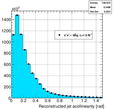
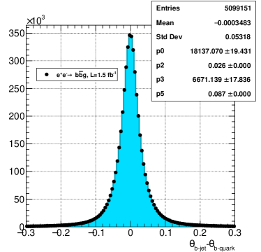
Figure 1: Left: acollinearity distribution between the two b-tagged reconstructed jets in selected $\mathrm{e^{+}e^{-}}\to{b\overline{b}(g)}$ events. Right: angular resolution on the original b-quark direction using reconstructed b-tagged jets, for an acollinearity cut of $\xi<0.3$. A fast simulation with DELPHES of an IDEA detector at the FCC-ee is used in the study .

The measured values of the asymmetry for different $\xi<\xi_{0}$ cuts are reported in Table 7 . The last column of the table contains the results after correction of the QCD shifts calculated at generator level (third column of Table 5). We observe that the measured asymmetry approaches with enough precision ${A_{FB}^{0}}$ at relatively low values of $\xi_{0}$, $\xi_{0}\approx 0.2-0.3$, for which QCD uncertainties should be almost negligible. There is a significant deviation from expectations for $\xi_{0}=0.1$. This value is not far from the estimated r.m.s. of the polar angle resolution, which may provoke distortions in the fitted distribution that we have not explored yet. Also, results for too low values of $\xi_{0}$ can be affected by intra-jet systematics that are difficult to evaluate at this stage.

$\xi_{0}$ cut	${A_{FB}}(\xi<\xi_{0})$	${A_{FB}}$ QCD-corrected
No cut	$0.0992\pm 0.0002(\mathrm{stat.})$	$0.1032\pm 0.0002(\mathrm{stat.})$
$1.50$	$0.0997\pm 0.0003(\mathrm{stat.})$	$0.1026\pm 0.0003(\mathrm{stat.})$
$1.00$	$0.1006\pm 0.0003(\mathrm{stat.})$	$0.1027\pm 0.0003(\mathrm{stat.})$
$0.50$	$0.1022\pm 0.0003(\mathrm{stat.})$	$0.1032\pm 0.0003(\mathrm{stat.})$
$0.30$	$0.1028\pm 0.0003(\mathrm{stat.})$	$0.1033\pm 0.0003(\mathrm{stat.})$
$0.20$	$0.1031\pm 0.0003(\mathrm{stat.})$	$0.1034\pm 0.0003(\mathrm{stat.})$
$0.10$	$0.1021\pm 0.0004(\mathrm{stat.})$	$0.1023\pm 0.0004(\mathrm{stat.})$

Table 7: Forward-backward asymmetry measured in $10^{7}$ simulated $\mathrm{e^{+}e^{-}}\to\mathrm{b\overline{b}}(\mathrm{g})$ events at ${\sqrt{s}}=91.2$ GeV, for different $\xi<\xi_{0}$ cuts between the two selected b-tagged reconstructed jets. The last column provides those asymmetry values corrected by QCD effects. The expected asymmetry in the absence of QCD corrections is: ${A_{FB}^{0}}=0.1036\pm 0.0003$. Only statistical uncertainties are shown.

6.3 Stability under hadronization and timelike-showering uncertainties

The same simplified study is repeated on 6 additional samples, generated according to the alternative shower tunes available in PYTHIA8 PYTHIA8 for $\mathrm{e^{+}e^{-}}$ collisions. Similarly to the reference study, 10 million $\mathrm{e^{+}e^{-}}\to\mathrm{b\overline{b}}(g)$ events at the Z pole were generated for each tune. For reference, the available choices are listed in Table 8.

Pythia8 $\mathrm{e^{+}e^{-}}$ tune	Description
1	the original PYTHIA 8 parameter set, based on some very old
	flavour studies (with JETSET around 1990) and a simple tune
	of ${\alpha_{s}}$ to three-jet shapes to the new $p_{T}$-ordered shower.
2	a tune by Marc Montull to the LEP 1 particle composition, as
	published in the RPP (August 2007). No related (re)tune to
	event shapes has been performed, however.
3	a tune to a wide selection of LEP1 data by Hendrik Hoeth
	within the Rivet + Professor framework, both to hadronization
	and timelike-shower parameters (June 2009).
4	a tune to LEP data by Peter Skands, by hand, both to
	hadronization and timelike-shower parameters (September 2013).
5	first tune to LEP data by Nadine Fischer (September 2013),
	based on the default flavour-composition parameters. Input
	is event shapes (ALEPH and DELPHI), identified particle
	spectra (ALEPH), multiplicities (PDG), and B hadron
	fragmentation functions (ALEPH).
6	second tune to LEP data by Nadine Fischer (September 2013).
	Similar to the first one, but event shapes are weighted up
	significantly, and multiplicities not included.
7	(default) the Monash 2013 tune by Peter Skands at al. MONASH-2013 , to
	both $\mathrm{e^{+}e^{-}}$ and $\mathrm{pp}/\mathrm{p\overline{p}}$ data.

Table 8: Available $\mathrm{e^{+}e^{-}}$ parton shower tune choices in Pythia8 PYTHIA8 .

We decouple the statistical fluctuations in the comparison between Pythia tunes by studying the changes in the ratio between the measured asymmetry at the reconstruction level and the bare asymmetry ${A_{FB}^{0}}$ calculated at the generator level on the same event sample:

$${\cal R}_{\text{QCD effects}}\equiv\left.\frac{{A_{FB}}(\text{measured})}{{A_{FB}^{0}}(\text{generator level})}\right|_{\text{same events}}\;.$$ (20)

${A_{FB}^{0}}$ is the asymmetry corrected by QED effects, without the inclusion of any QCD corrections, and its central value is unaffected by acollinearity cuts within the targeted precision. Therefore, the proposed ratio tracks in the most precise way distortions of the asymmetry that are exclusively due to QCD effects.

With this new definition in hand we are now able to understand in more depth the evolution of the asymmetry measurement as a function of the $\xi_{0}$ cut applied at the reconstruction level. The central values of the measurement are obtained by scaling the ratio ${\cal R}_{\text{QCD effects}}$ at each point by the factor ${A_{FB}^{0}}=0.10379\pm 0.00011(\mathrm{stat.})$, determined using all the available statistics. Regarding uncertainties, three separate components are considered at each $\xi_{0}$ point: 1) the statistical uncertainty provided by the weighted average of the 7 tune results, basically corresponding to $1/\sqrt{7}$ times the uncertainties reported in Table 7 for the Monash 2013 tune case; 2) the (symmetrized) envelope of the central results obtained using different tunes; 3) a theoretical uncertainty equivalent to a $10\%$ relative uncertainty on the correction factor $C$, consistent with the uncertainty assumed in LEP measurements lephf-05 . Central values and uncertainties are collected in Table 9, and depicted in Figure 2. Results are also corrected for small biases due to the limited angular resolution effects, as discussed in Section 8.

$\xi_{0}$ cut	Measured ${A_{FB}}$	$\Delta{A_{FB}}(\text{stat})$	$\Delta{A_{FB}}(\text{tune})$	$\Delta{A_{FB}}(\text{theo. QCD corr})$
No cut	$0.0998\pm 0.0004$	$0.00008$	$0.00014$	$0.00033$
$1.50$	$0.1003\pm 0.0003$	$0.00011$	$0.00014$	$0.00023$
$1.00$	$0.1011\pm 0.0002$	$0.00011$	$0.00010$	$0.00016$
$0.50$	$0.1023\pm 0.0002$	$0.00011$	$0.00010$	$0.00007$
$0.30$	$0.1030\pm 0.0002$	$0.00011$	$0.00010$	$0.00003$
$0.20$	$0.1033\pm 0.0001$	$0.00011$	$0.00005$	$0.00002$
$0.10$	$0.1035\pm 0.0002$	$0.00016$	$0.00005$	$0.00001$

Table 9: Central values and components of the uncertainty in the measurement of the ${A_{FB}}$ asymmetry with $7\times 10^{7}$ $\mathrm{e^{+}e^{-}}\to\mathrm{b\overline{b}}(\mathrm{g})$ events at the Z pole, for different $\xi<\xi_{0}$ cuts at the reconstructed level.

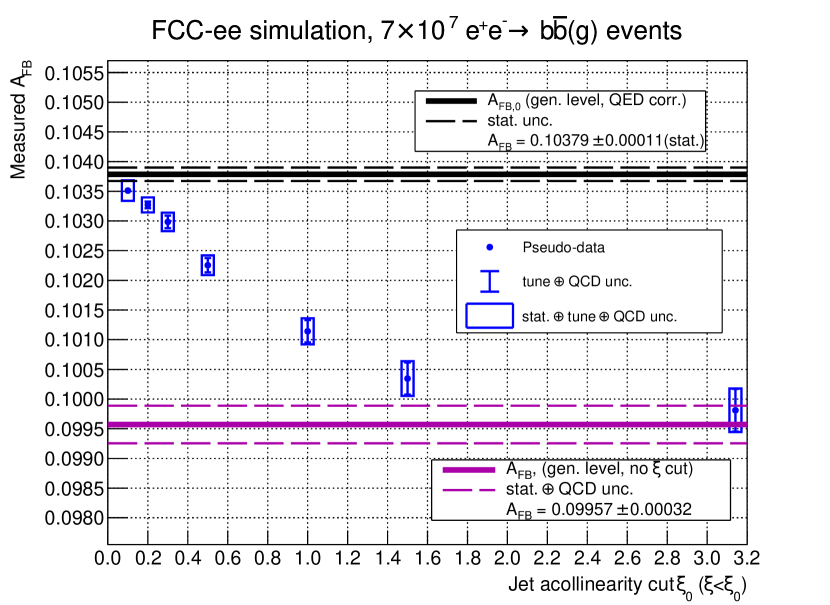
Figure 2: Evolution of the expected measurement of the asymmetry in $7\times 10^{7}\mathrm{e^{+}e^{-}}\to\mathrm{b\overline{b}}(\mathrm{g})$ simulated events at ${\sqrt{s}}=91.2$ GeV as a function of the acollinearity cut $\xi<\xi_{0}$. The systematic uncertainties in the pseudo-data points take into account the envelope of the results obtained using different PYTHIA8 tunes, which define the hadronization and timelike-showering properties in the event generation. These results indicate that cuts in the range $\xi_{0}=0.2-0.3$ should minimize the overall uncertainty. The generator-level values of the asymmetries without and with QCD corrections in the absence of acollinearity cuts are also shown for reference.

Changes in the central values of the asymmetry as a function of the acollinearity cut can be largely explained by the different size of the theoretically expected QCD corrections at each point. The uncertainty on these corrections is larger ($\Delta{A_{FB}}(\text{QCD corr})\approx 0.0003$) when no acollinearity cuts are applied. Pythia tune uncertainties seem to have a marginal effect for $\xi_{0}<0.5$ ($\Delta{A_{FB}}(\text{tune})\lesssim 0.0001$) and are relatively stable down to rather low values of the acollinearity cut. Statistical uncertainties start to dominate for $\xi_{0}\lesssim 0.3$, but let us remind that the statistical uncertainty will not be a limiting factor at FCCee, where $\approx 10^{12}$ Z decays should be available. We conclude that, for a real analysis of $\mathrm{e^{+}e^{-}}\to\mathrm{b\overline{b}}(\mathrm{g})$ events, a cut $\xi<0.2-0.3$ is already optimal, with associated QCD systematics $\Delta{A_{FB}}(\text{tune+QCD corr})\lesssim 0.0001$.

Figure 2 also shows the generator-level reference values of the asymmetry with and without QCD corrections, calculated in the absence of acollinearity cuts. Let us note again that we only expect a qualitative agreement with the reference value with QCD corrections. For instance, there are hidden implicit cuts on acollinearity at the selection level. We consider reconstructed jets with a limited resolution parameter ($0.4$), but require at least two tagged b-jets in the event. Even without any explicit cut, the double-tag requirement rejects events in which bottom and antibottom quarks are in the same jet. Moreover, this region of phase space is affected by gluon splitting contamination, something difficult to reproduce in simulations. All of this encourages even further the use of explicit acollinearity cuts and double flavor tagging in the analysis before estimation of any QCD corrections.

7 QCD uncertainties and b semileptonic decays

One of the proposals to reduce QCD uncertainties was the one discussed in Reference ep-98 . The authors of the study analyzed the evolution of the QCD corrections as a function of the momentum and the transverse momentum of leptons (with respect to the associated jet direction) in b decays. The corrections are quantified in terms of the parameter $C_{b}=\frac{{\alpha_{s}}}{\pi}~{}C$ or, equivalently:

$$C_{b} \equiv 1-\frac{{A_{FB}}}{{A_{FB}^{0}}}\;.$$ (21)

We estimate $C_{b}$ using the $7\times 10^{7}$ simulated events analyzed in Section 6.3. In order to be more consistent with the analysis of Reference ep-98 , we select events with a charged lepton in the final state at generator level with momentum larger than 3 GeV. The results are shown if Figure 3. The central values of $C_{b}$ in each bin are obtained as the average of the estimates of the 7 different Pythia tune samples, while uncertainties are derived from the root-mean-square deviation of these estimates. Our findings are qualitatively consistent with those reported in ep-98 , except at large values the transverse momentum, probably due to the presence of looser requirements in the angular association between lepton and jet for the present study.

The results are easily interpreted in terms of the acollinearity discussion of the previous sections. Tight cuts on the lepton momentum reduce significantly the number of events with hard gluon radiation close to that jet and, as a consequence, increase the number of collinear events. But the reduction is less effective than the one using explicit acollinearity cuts, simply due to the absence of requirements on the opposite jet. This is visually shown in Figure 4, using the same scale for comparison. Here we require in addition the presence of two reconstructed b-tagged jets with an acollinearity cut of $\xi<0.3$. The size of the QCD corrections gets significantly reduced. Also as expected, tight cuts on transverse momentum lead to an increase in the size of QCD corrections: low values are more consistent with a collinear configuration (low values of $C_{b}$), while high values of transverse momentum favor configurations with hard gluon emission away from the jet, as also observed by the authors of the original study ep-98 .

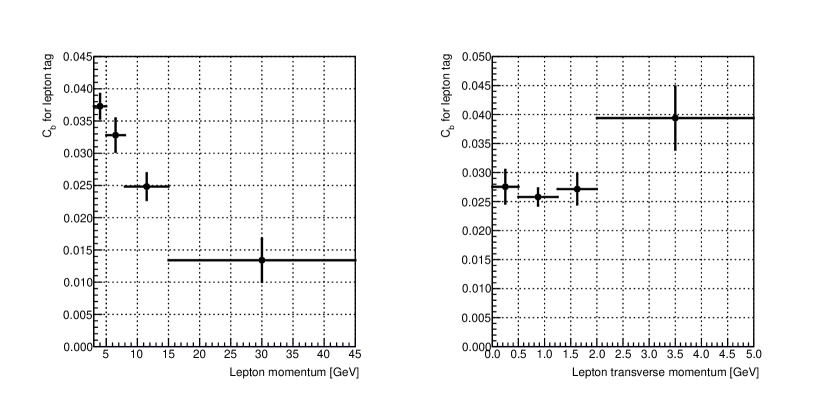
Figure 3: QCD corrections factors $C_{b}$ in events with charged leptons in the final state. Only leptons with a momentum larger than 3 GeV are considered in the estimates. The results are presented as a function of the lepton momentum and transverse momentum with respect to the closest b-tagged jet direction. The central values of $C_{b}$ in each bin are obtained as the average of the estimates of the 7 different Pythia tune samples, while uncertainties are derived from the root-mean-square deviation of these estimates.

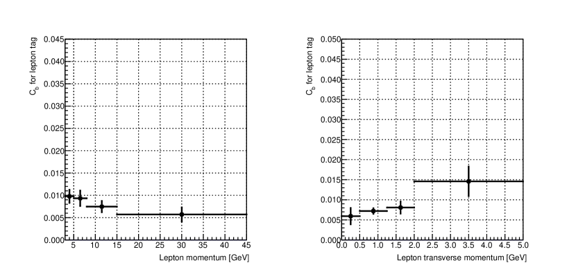
Figure 4: QCD corrections factors $C_{b}$ in events with charged leptons in the final state. Only leptons with a momentum larger than 3 GeV are considered in the estimates. We require in addition the presence of two reconstructed b-tagged jets with an acollinearity cut $\xi<0.3$. The results are presented as a function of the lepton momentum and transverse momentum with respect to the closest b-tagged jet direction. The central values of $C_{b}$ in each bin are obtained as the average of the estimates of the 7 different Pythia tune samples, while uncertainties are derived from the root-mean-square deviation of these estimates.

8 Biases in the measurement of the asymmetry. Choice of the differential angular distribution.

Biases in the measurement of forward-backward asymmetries are intrinsically small. Efficiency losses increase the statistical uncertainty of the measurement, but do not bias it, as long as they are independent of charge and a proper fit method is used. However, at the level of the precision expected at future colliders, a real study with data will have to carefully include all potential sources of bias. Here we will focus in the particular case of ${A_{FB}^{0,b}}$, but similar considerations are applicable to the case of charm quarks. We will distinguish four different types of bias: 1) charge confusion effects, like B-mixing or experimental charge misidentification; 2) angular distortions, and in particular the effect of a limited angular resolution; 3) background contamination (mostly charm and light quarks) ; 4) wrong description of the polar angular distribution.

Charge confusion leads to a dilution of the asymmetry. The functional form of the angular distribution does not change if the charge confusion has no significant angular dependence:

$$\frac{d\rho}{d\cos\theta_{b}} = \frac{1}{1+f_{L}}~{}\left[\frac{3}{8}~{}(1+\cos^{2}\theta_{b})+\frac{3}{4}~{}f_{L}\sin^{2}\theta_{b}\right]+{A^{\prime}_{FB}}~{}\cos\theta_{b}\;,$$ (22)

${A^{\prime}_{FB}}$ must be corrected a posteriori to obtain the true value of the asymmetry. Assuming a fraction $\chi$ of events with the wrong charge: ${A^{\prime}_{FB}}=(1-2\chi)~{}{A_{FB}}$. In the more general case of a symmetric dependence with the polar angle: $\chi\equiv\chi(|\cos\theta_{b}|)$, a slightly different distribution must be used:

$$\frac{d\rho}{d\cos\theta_{b}} = \frac{1}{1+f_{L}}~{}\left[\frac{3}{8}~{}(1+\cos^{2}\theta_{b})+\frac{3}{4}~{}f_{L}\sin^{2}\theta_{b}\right]+{A_{FB}}~{}[1-2\chi(|\cos\theta_{b}|)]~{}\cos\theta_{b}\;.$$ (23)

The function $\chi(|\cos\theta_{b}|)$ can be extracted either from simulations or from dedicated studies in control data samples. It can also be directly measured from a global data fit with multiple charge and flavor tags. The remaining biases are expected to be small. At LEP, B-mixing was already an almost negligible source of systematic uncertainty in the combined measurement ($\Delta{A_{FB}^{0,b}}\approx 0.0001$). Detector-related charge confusion effects can be estimated in control samples with double tagging of the charge, and is expected a priori to be small in several cases of interest, like measurements that use exclusive decays or inclusive semi-leptonic b decays lephf-05 .

The limited angular resolution in the polar angle, ${\sigma_{\theta}}$, is intrinsically a source of a bias in the measurement. Any value of ${\sigma_{\theta}}>0$ flattens the original angular distribution and results into a lower absolute value of the fitted asymmetry. To illustrate the effect of a typical jet resolution we generate a toy sample of $10^{9}$ events with the resolution parameters extracted from Figure 1-right of Section 6.2, for an acollinearity cut of $\xi<0.3$. We perform a likelihood fit to the usual angular distribution (which assumes ${\sigma_{\theta}}=0$) in the fiducial volume $|\cos\theta_{b}|<0.97$, consistent with the tracker acceptance of the IDEA detector. The result is a relatively small shift of $\Delta{A_{FB}}=-0.000195\pm 0.000014$, which is used to correct the results obtained with likelihood fits in previous sections. Let us note that the angular resolution can still be improved by combining the jet angular information with the measurement of the direction of the secondary vertex, which is much closer to the original b-quark direction. Nevertheless, we conclude that angular resolution effects should be studied and carefully corrected in a real analysis.

For the b-quark asymmetry, and at the level of the aimed precision, the contamination from charm and light quarks can be estimated in situ using control samples, or even extracted directly from data. A very precise extraction of the background will likely require an extension to double flavor-tag methods, the addition of flavor-sensitive variables, and the formulation of complicated probability density functions to appropriately describe all the flavor components. In any case, in LEP combinations the effect of uncertainties in the background composition was already minor: $\Delta{A_{FB}}\approx 0.0001$ lephf-05 . Improved heavy-quark tagging capabilities and the larger collected statistics at future colliders should provide an even better control of these contributions. Also, with $\approx 10^{12}$ Z decays, one could envisage measurements using only a few exclusive channels. For instance, $\approx 10^{8}$ $\mathrm{B}^{+}$ decays will be available Fabrizio for a measurement minimally affected by B-mixing, charm/light background or charge confusion.

The last source of bias that we consider is the choice of the angular distribution used to fit the asymmetry. A measurement with huge statistics will certainly demand careful tests of its validity. For instance, a measurable longitudinal component due to new physics can not be excluded a priori, given the level of precision. An example would be the exchange of a scalar particle in the s-channel with sizable couplings to electrons and heavy quarks or, in a more generic way, the presence of an effective interaction of the $(\overline{\mathrm{e}}_{L}\mathrm{e}_{R})(\overline{\mathrm{b}}_{L}\mathrm{b}_{R})$ type. In this context, one could even envisage a fit with two parameters, $f_{L}$ and ${A_{FB}}$, using Equation 23 above.

Finally, we should point out that the usual description in terms of Z decay angular components is not strictly valid when higher-order electroweak corrections are taken into account. This is simply a manifestation of quantum interference effects between Z production and Z decay terms in the ${\mathrm{e^{+}e^{-}}\to Q\overline{Q}(g)}$ process. Even if these interference effects are expected to be negligible at the Z pole, they become larger as we move away from this energy point. As an example, initial-final state QED interference effects, critical for a precise measurement of the asymmetry in the $\mathrm{e^{+}e^{-}}\to\mu^{+}\mu^{-}(\gamma)$ process, have been investigated in Reference Jadach:2018lwm . The conclusion is that effects as large as $1\%$ can be present at energies a few GeV above the Z mass. In practice, accounting for these effects should not be extremely problematic. One can assume a more general polar angle distribution, with symmetric and antisymmetric density terms $\mathcal{S}(\cos^{2}\theta_{b})$ and $\mathcal{A}(\cos\theta_{b})$, and properly normalized such that:

$$\frac{d\rho}{d\cos\theta_{b}} = \mathcal{S}(\cos^{2}\theta_{b})+{A_{FB}}~{}\mathcal{A}(\cos\theta_{b})\;.$$ (24)

The exact values of the density terms as a function of $\cos\theta_{b}$ can be even obtained from analytical theory calculations. The solution of the unbinned likelihood fit to this distribution is:

$$v_{i}\equiv\frac{\mathcal{A}(\cos\theta_{b}{{}_{,i}})}{\mathcal{S}(\cos^{2}\theta_{b}{{}_{,i}})} \Rightarrow \sum_{i=1}^{N_{events}}\left(\frac{v_{i}}{1+{A_{FB}}~{}v_{i}}\right)=0\;,$$ (25)

which is still unbiased with respect to acceptance variations that are charge symmetric. The consistency of the functional form can be confirmed a posteriori through a study of the dependence with $|v|$ of the following function:

$$f(|v|) = {\displaystyle\frac{\left[dN(|v|)-dN(-|v|)\right]}{\left[dN(|v|)+dN(-|v|)\right]}}\;,$$ (26)

where $dN(x)$ is the number of selected events in the $(x-\frac{dx}{2},x+\frac{dx}{2})$ interval. If the functional form is appropriate then one expects a good fit of the histogram of $f(|v|)$ versus $|v|$ to the linear relation: $f(|v|)={A_{FB}}~{}|v|$. Actually, an alternative value of ${A_{FB}}$ can be extracted from this fit. Note however that the resulting statistical uncertainty will be by construction larger than the optimal one, which is given by the unbinned maximum likelihood fit described before.

9 Outlook

Using existing theoretical calculations as a starting point we have derived simple expressions for the QCD corrections to the measurement of the forward-backward asymmetry of the ${\mathrm{e^{+}e^{-}}\to Q\overline{Q}(g)}$ process at ${\sqrt{s}}=m_{\mathrm{Z}}$. We show that these QCD corrections and uncertainties can be reduced by almost one order of magnitude using simple acollinearity cuts between the heavy quarks. The inclusion of hadronization and final-state parton shower effects does not modify this picture. These findings are also enough to explain the behavior of other observables previously suggested for a partial mitigation of QCD effects. The proposed strategy is a first step towards a measurement of the heavy-quark forward-backward asymmetry with systematic uncertainties of order $\Delta{A_{FB}^{0,Q}}\approx 10^{-4}$. Focusing on the case of b quarks, it is found that other possible sources of bias in the measurement of the asymmetry could be controlled at that level of precision using current theoretical knowledge, adequate fitting techniques and an appropriate choice of data control samples.

References

- (1) ALEPH, DELPHI, L3, OPAL, SLD, LEP Electroweak Working Group, SLD Electroweak Group, SLD Heavy Flavour Group, S. Schael et al., “Precision electroweak measurements on the resonance”, Phys. Rept. 427 (2006) 257–454, arXiv:hep-ex/0509008.
- (2) A. Djouadi, G. Moreau, and F. Richard, “Resolving the A(FB)**b puzzle in an extra dimensional model with an extended gauge structure”, Nucl. Phys. B 773 (2007) 43–64, arXiv:hep-ph/0610173.
- (3) LEP Heavy Flavor Working Group, D. Abbaneo, P. Antilogus, T. Behnke, S. Blyth, M. Elsing, R. Faccini, R. Jones, K. Monig, S. Petzold, and R. Tenchini, “QCD corrections to the forward - backward asymmetries of c and b quarks at the Z pole”, Eur. Phys. J. C 4 (1998) 185–191.
- (4) D. d’Enterria and C. Yan, “Forward-backward -quark asymmetry at the Z pole: QCD uncertainties redux”, in 53rd Rencontres de Moriond on QCD and High Energy Interactions, pp. 253–257. 2018. arXiv:1806.00141 [hep-ex].
- (5) J. Jersak, E. Laermann, and P. Zerwas, “Electroweak Production of Heavy Quarks in e+ e- Annihilation”, Phys. Rev. D 25 (1982) 1218. [Erratum: Phys.Rev.D 36, 310 (1987)].
- (6) A. Djouadi, J. H. Kuhn, and P. Zerwas, “B Jet Asymmetries in Z Decays”, Z. Phys. C 46 (1990) 411–418.
- (7) A. Arbuzov, D. Bardin, and A. Leike, “Analytic final state corrections with cut for e+ e- —> massive fermions”, Mod. Phys. Lett. A 7 (1992) 2029–2038. [Erratum: Mod.Phys.Lett.A 9, 1515 (1994)].
- (8) A. Djouadi, B. Lampe, and P. Zerwas, “A Note on the QCD corrections to forward - backward asymmetries of heavy quark jets in Z decays”, Z. Phys. C 67 (1995) 123–128, arXiv:hep-ph/9411386.
- (9) G. Altarelli and B. Lampe, “Second order QCD corrections to heavy quark forward - backward asymmetries”, Nucl. Phys. B 391 (1993) 3–22.
- (10) J. Stav and H. Olsen, “Radiative gluon effects in massive quark anti-quark production in collisions of positrons and polarized electrons at the Z0 resonance”, Phys. Rev. D 52 (1995) 1359–1368.
- (11) V. Ravindran and W. van Neerven, “Second order QCD corrections to the forward - backward asymmetry in e+ e- collisions”, Phys. Lett. B 445 (1998) 214–222, arXiv:hep-ph/9809411.
- (12) S. Catani and M. H. Seymour, “Corrections of O (alpha-S**2) to the forward backward asymmetry”, JHEP 07 (1999) 023, arXiv:hep-ph/9905424.
- (13) S. Weinzierl, “The Forward-backward asymmetry at NNLO revisited”, Phys. Lett. B 644 (2007) 331–335, arXiv:hep-ph/0609021.
- (14) W. Bernreuther, L. Chen, O. Dekkers, T. Gehrmann, and D. Heisler, “The forward-backward asymmetry for massive bottom quarks at the peak at next-to-next-to-leading order QCD”, JHEP 01 (2017) 053, arXiv:1611.07942 [hep-ph].
- (15) FCC, A. Abada et al., “FCC-ee: The Lepton Collider: Future Circular Collider Conceptual Design Report Volume 2”, Eur. Phys. J. ST 228 no. 2, (2019) 261–623.
- (16) A. Banfi, G. P. Salam, and G. Zanderighi, “Infrared safe definition of jet flavor”, Eur. Phys. J. C 47 (2006) 113–124, arXiv:hep-ph/0601139.
- (17) DELPHES 3, J. de Favereau, C. Delaere, P. Demin, A. Giammanco, V. Lemaître, A. Mertens, and M. Selvaggi, “DELPHES 3, A modular framework for fast simulation of a generic collider experiment”, JHEP 02 (2014) 057, arXiv:1307.6346 [hep-ex].
- (18) T. Sjostrand, S. Mrenna, and P. Z. Skands, “PYTHIA 6.4 Physics and Manual”, JHEP 05 (2006) 026, arXiv:hep-ph/0603175.
- (19) T. Sjostrand, S. Mrenna, and P. Z. Skands, “A Brief Introduction to PYTHIA 8.1”, Comput. Phys. Commun. 178 (2008) 852–867, arXiv:0710.3820 [hep-ph].
- (20) P. Skands, S. Carrazza, and J. Rojo, “Tuning PYTHIA 8.1: the Monash 2013 Tune”, Eur. Phys. J. C 74 no. 8, (2014) 3024, arXiv:1404.5630 [hep-ph].
- (21) M. Cacciari, G. P. Salam, and G. Soyez, “FastJet User Manual”, Eur. Phys. J. C 72 (2012) 1896, arXiv:1111.6097 [hep-ph].
- (22) F. Palla, “Challenges for EW b physics measurements”, talk at the FCC Week 2019, Brussels, 25 June 2019 . https://indico.cern.ch/event/727555/contributions/3446561/.
- (23) S. Jadach and S. Yost, “QED Interference in Charge Asymmetry Near the Z Resonance at Future Electron-Positron Colliders”, Phys. Rev. D 100 no. 1, (2019) 013002, arXiv:1801.08611 [hep-ph].