A Sampling-Based Method for Tensor Ring Decomposition

Supplementary Material

Abstract

We propose a sampling-based method for computing the tensor ring (TR) decomposition of a data tensor. The method uses leverage score sampled alternating least squares to fit the TR cores in an iterative fashion. By taking advantage of the special structure of TR tensors, we can efficiently estimate the leverage scores and attain a method which has complexity sublinear in the number of input tensor entries. We provide high-probability relative-error guarantees for the sampled least squares problems. We compare our proposal to existing methods in experiments on both synthetic and real data. Our method achieves substantial speedup—sometimes two or three orders of magnitude—over competing methods, while maintaining good accuracy. We also provide an example of how our method can be used for rapid feature extraction.

1 Introduction

Tensor decomposition has recently found many applications in machine learning and related areas. Examples include parameter reduction in neural networks (Novikov et al., 2015; Garipov et al., 2016; Yang et al., 2017; Yu et al., 2017; Ye et al., 2018), understanding the expressivity of deep neural networks (Cohen et al., 2016; Khrulkov et al., 2018), supervised learning (Stoudenmire & Schwab, 2017; Novikov et al., 2017), filter learning (Hazan et al., 2005; Rigamonti et al., 2013), image factor analysis and recognition (Vasilescu & Terzopoulos, 2002; Liu et al., 2019), scaling up Gaussian processes (Izmailov et al., 2018), multimodal feature fusion (Hou et al., 2019), natural language processing (Lei et al., 2014), data mining (Papalexakis et al., 2016), feature extraction (Bengua et al., 2015), and tensor completion (Wang et al., 2017). The CP and Tucker decompositions are the two most popular tensor decompositions that each have strengths and weaknesses (Kolda & Bader, 2009). The number of parameters in the CP decomposition scales linearly with the tensor dimension, but finding a good decomposition numerically can be challenging. The Tucker decomposition is usually easier to work with numerically, but the number of parameters grows exponentially with tensor dimension. To address these challenges, decompositions based on tensor networks have recently gained in popularity. The tensor train (TT) is one such decomposition (Oseledets, 2011). The number of parameters in a TT scales linearly with the tensor dimension. The tensor ring (TR) decomposition is a generalization of the TT decomposition. It is more expressive than the TT decomposition (see Remark 1), but maintains the linear scaling of the number of parameters with increased tensor dimension. Although the TR decomposition is known to have certain numerical stability issues it usually works well in practice, achieving a better compression ratio and lower storage cost than the TT decomposition (Mickelin & Karaman, 2020).

It is crucial to have efficient algorithms for computing the decomposition of a tensor. This task is especially challenging for large and high-dimensional tensors. In this paper, we present a sampling-based method for TR decomposition which has complexity sublinear in the number of input tensor entries. The method fits the TR core tensors by iteratively updating them in an alternating fashion. Each update requires solving a least squares problem. We use leverage score sampling to speed up the solution of these problems and avoid having to consider all elements in the input tensor for each update. The system matrices in the least squares problems have a particular structure that we take advantage of to efficiently estimate the leverage scores. To summarize, we make the following contributions:

• Propose a sampling-based method for TR decomposition which has complexity sublinear in the number of input tensor entries.

• Provide relative-error guarantees for the sampled least squares problems we use in our algorithm.

• Compare our proposed algorithm to four other methods in experiments on both synthetic and real data.

• Provide an example of how our method can be used for rapid feature extraction.

2 Related Work

Leverage score sampling has been used previously for tensor decomposition. Cheng et al. (2016) use it to reduce the size of the least squares problems that come up in the alternating least squares (ALS) algorithm for CP decomposition. They efficiently estimate the leverage scores by exploiting the Khatri–Rao structure of the design matrices in these least squares problems and prove additive-error guarantees. Larsen & Kolda (2020) further improve this method by combining repeatedly sampled rows and by using a hybrid deterministic–random sampling scheme. These techniques make the method faster without sacrificing accuracy. Our paper differs from these previous works since we consider a different kind of tensor decomposition. Since the TR decomposition has core tensors instead of factor matrices, the leverage score estimation formulas used in the previous works cannot be used for TR decomposition.

There are previous works that develop randomized algorithms for TR decomposition. Yuan et al. (2019) develop a method which first applies a randomized variant of the HOSVD Tucker decomposition, followed by a TR decomposition of the core tensor using either a standard SVD- or ALS-based algorithm. Finally, the TR cores are contracted appropriately with the Tucker factor matrices to get a TR decomposition of the original tensor. Ahmadi-Asl et al. (2020) present several TR decomposition algorithms that incorporate randomized SVD. In Section 5, we compare our proposed algorithm to methods by Yuan et al. (2019) and Ahmadi-Asl et al. (2020) in experiments.

Papers that develop randomized algorithms for other tensor decompositions include the works by Wang et al. (2015), Battaglino et al. (2018), Yang et al. (2018) and Aggour et al. (2020) for the CP decomposition; Biagioni et al. (2015) and Malik & Becker (2020) for tensor interpolative decomposition; Drineas & Mahoney (2007), Tsourakakis (2010), da Costa et al. (2016), Malik & Becker (2018), Sun et al. (2020) and Minster et al. (2020) for the Tucker decomposition; Zhang et al. (2018) and Tarzanagh & Michailidis (2018) for t-product-based decompositions; and Huber et al. (2017) and Che & Wei (2019) for the TT decomposition.

Skeleton approximation and other sampling-based methods for TR decomposition include the works by Espig et al. (2012) and Khoo et al. (2019). Espig et al. (2012) propose a skeleton/cross approximation type method for the TR format with complexity linear in the dimensionality of the tensor. Khoo et al. (2019) propose an ALS-based scheme for constructing a TR decomposition based on only a few samples of the input tensor. Papers that use skeleton approximation and sampling techniques for other types of tensor decomposition include those by Mahoney et al. (2008), Oseledets et al. (2008), Oseledets & Tyrtyshnikov (2010), Caiafa & Cichocki (2010), and Friedland et al. (2011).

3 Preliminaries

By tensor, we mean a multidimensional array of real numbers. Boldface Euler script letters, e.g. $\boldsymbol{\mathscr{X}}$, denote tensors of dimension 3 or greater; bold uppercase letters, e.g. $\bm{X}$, denote matrices; bold lowercase letters, e.g. $\bm{x}$, denote vectors; and regular lowercase letters, e.g. $x$, denote scalars. Elements of tensors, matrices and vectors are denoted in parentheses. For example, $\boldsymbol{\mathscr{X}}(i_{1},i_{2},i_{3})$ is the element on position $(i_{1},i_{2},i_{3})$ in the 3-way tensor $\boldsymbol{\mathscr{X}}$, and $\bm{y}(i_{1})$ is the element on position $i_{1}$ in the vector $\bm{y}$. A colon is used to denote all elements along a dimension. For example, $\bm{X}(i,:)$ denotes the $i$th row of the matrix $\bm{X}$. For a positive integer $I$, define $[I]\stackrel{{\scriptstyle\text{\tiny{def}}}}{{=}}\{1,\ldots,I\}$. For indices $i_{1}\in[I_{1}],\ldots,i_{N}\in[I_{N}]$, the notation $\overline{i_{1}i_{2}\cdots i_{N}}\stackrel{{\scriptstyle\text{\tiny{def}}}}{{=}}\sum_{n=1}^{N}i_{n}\prod_{j=1}^{n-1}I_{j}$ will be helpful when working with reshaped tensors. $\|\cdot\|_{\textup{F}}$ denotes the Frobenius norm of matrices and tensors, and $\|\cdot\|_{2}$ denotes the Euclidean norm of vectors.

3.1 Tensor Ring Decomposition

Let $\boldsymbol{\mathscr{X}}\in\mathbb{R}^{I_{1}\times\cdots\times I_{N}}$ be an $N$-way tensor. For $n\in[N]$, let $\boldsymbol{\mathscr{G}}^{(n)}\in\mathbb{R}^{R_{n-1}\times I_{n}\times R_{n}}$ be 3-way tensors with $R_{0}=R_{N}$. A rank-$(R_{1},\ldots,R_{N})$ TR decomposition of $\boldsymbol{\mathscr{X}}$ takes the form

$$\boldsymbol{\mathscr{X}}(i_{1},\ldots,i_{N})=\sum_{r_{1},\ldots,r_{N}}\prod_{n=1}^{N}\boldsymbol{\mathscr{G}}^{(n)}(r_{n-1},i_{n},r_{n}),$$ (1)

where each $r_{n}$ in the sum goes from $1$ to $R_{n}$ and $r_{0}=r_{N}$. $\boldsymbol{\mathscr{G}}^{(1)},\ldots,\boldsymbol{\mathscr{G}}^{(N)}$ are called core tensors. We will use $\operatorname*{\operatorname{TR}}((\boldsymbol{\mathscr{G}}^{(n)})_{n=1}^{N})$ to denote a tensor ring with cores $\boldsymbol{\mathscr{G}}^{(1)},\ldots,\boldsymbol{\mathscr{G}}^{(N)}$. The name of the decomposition comes from the fact that it looks like a ring in tensor network notation; see Figure 1. The TT decomposition is a special case of the TR decomposition with $R_{0}=R_{N}=1$, which corresponds to severing the connection between $\boldsymbol{\mathscr{G}}^{(1)}$ and $\boldsymbol{\mathscr{G}}^{(5)}$ in Figure 1. The TR decomposition can therefore also be interpreted as a sum of tensor train decompositions with the cores $\boldsymbol{\mathscr{G}}^{(2)},\ldots,\boldsymbol{\mathscr{G}}^{(N-1)}$ in common.

Remark 1 (Expressiveness of TR vs TT).

Since the TT decomposition is a special case of the TR decomposition, any TT is also a TR with the same number of parameters. So the TR decomposition is at least as expressive as the TT decomposition. To see that the TR decomposition is strictly more expressive than the TT decomposition, consider the following example: Let $\boldsymbol{\mathscr{X}}=\operatorname*{\operatorname{TR}}(\boldsymbol{\mathscr{G}},\boldsymbol{\mathscr{G}},\boldsymbol{\mathscr{G}},\boldsymbol{\mathscr{G}})$ where $\boldsymbol{\mathscr{G}}\in\mathbb{R}^{2\times 2\times 2}$ has entries $1,2,\ldots,8$ ($\boldsymbol{\mathscr{G}}=\verb|reshape(1:8,2,2,2)|$ in Matlab). This TR of $\boldsymbol{\mathscr{X}}$ requires $4\cdot(2\cdot 2\cdot 2)=32$ parameters. The TT ranks of $\boldsymbol{\mathscr{X}}$ are $(2,4,2)$ (computed via Theorem 8.8 by Ye & Lim (2018)). An exact TT decomposition of $\boldsymbol{\mathscr{X}}$ therefore requires $2\cdot(2\cdot 2)+2\cdot(2\cdot 2\cdot 4)=40$ parameters.

Figure 1: Tensor ring decomposition of $5$-way tensor.

The problem of fitting $\operatorname*{\operatorname{TR}}((\boldsymbol{\mathscr{G}}^{(n)})_{n=1}^{N})$ to a data tensor $\boldsymbol{\mathscr{X}}$ can be written as the minimization problem

$$\operatorname*{arg\,min}_{\boldsymbol{\mathscr{G}}^{(1)},\ldots,\boldsymbol{\mathscr{G}}^{(N)}}\|\operatorname*{\operatorname{TR}}((\boldsymbol{\mathscr{G}}^{(n)})_{n=1}^{N})-\boldsymbol{\mathscr{X}}\|_{\textup{F}},$$ (2)

where the size of each core tensor is fixed. There are two common approaches to this fitting problem: one is SVD based and the other uses ALS. We describe the latter below since it is what we use in our work, and refer to Zhao et al. (2016) and Mickelin & Karaman (2020) for a description of the SVD-based approach.

Definition 2.

The classical mode-$n$ unfolding of $\boldsymbol{\mathscr{X}}$ is the matrix $\bm{X}_{(n)}\in\mathbb{R}^{I_{n}\times\prod_{j\neq n}I_{j}}$ defined elementwise via

$$\bm{X}_{(n)}(i_{n},\overline{i_{1}\cdots i_{n-1}i_{n+1}\cdots i_{N}})\stackrel{{\scriptstyle\text{\tiny{def}}}}{{=}}\boldsymbol{\mathscr{X}}(i_{1},\ldots,i_{N}).$$ (3)

The mode-$n$ unfolding of $\boldsymbol{\mathscr{X}}$ is the matrix $\bm{X}_{[n]}\in\mathbb{R}^{I_{n}\times\prod_{j\neq n}I_{j}}$ defined elementwise via

$$\bm{X}_{[n]}(i_{n},\overline{i_{n+1}\cdots i_{N}i_{1}\cdots i_{n-1}})\stackrel{{\scriptstyle\text{\tiny{def}}}}{{=}}\boldsymbol{\mathscr{X}}(i_{1},\ldots,i_{N}).$$ (4)

Definition 3.

By merging all cores except the $n$th, we get a subchain tensor $\boldsymbol{\mathscr{G}}^{\neq n}\in\mathbb{R}^{R_{n}\times\prod_{j\neq n}I_{j}\times R_{n-1}}$ defined elementwise via

$$\boldsymbol{\mathscr{G}}^{\neq n}(r_{n},\overline{i_{n+1}\ldots i_{N}i_{1}\ldots i_{n-1}},r_{n-1})$$ (5)

$$\stackrel{{\scriptstyle\text{\tiny{def}}}}{{=}}\sum_{\begin{subarray}{c}r_{1},\ldots,r_{n-2}\\ r_{n+1},\ldots,r_{N}\end{subarray}}\prod_{\begin{subarray}{c}j=1\\ j\neq n\end{subarray}}^{N}\boldsymbol{\mathscr{G}}^{(j)}(r_{j-1},i_{j},r_{j}).$$

It follows directly from Theorem 3.5 in Zhao et al. (2016) that the objective in (2) can be rewritten as

$$\|\operatorname*{\operatorname{TR}}((\boldsymbol{\mathscr{G}}^{(n)})_{n=1}^{N})-\boldsymbol{\mathscr{X}}\|_{\textup{F}}=\|\bm{G}_{[2]}^{\neq n}\bm{G}_{(2)}^{(n)\top}-\bm{X}_{[n]}^{\top}\|_{\textup{F}}.$$ (6)

The ALS approach to finding an approximate solution to (2) is to keep all cores except the $n$th fixed and solve the least squares problem above with respect to that core, and then repeat this multiple times for each $n\in[N]$ until some termination criterion is met. We summarize the approach in Algorithm 1. The initialization on line 1 can be done by, e.g., drawing each core entry independently from a standard normal distribution. Notice that the first core does not need to be initialized since it will be immediately updated. Normalization steps can also be added to the algorithm, but such details are omitted here. Throughout this paper we make the reasonable assumption that $\boldsymbol{\mathscr{G}}^{\neq n}\neq\bm{0}$ for all $n\in[N]$ during the execution of the ALS-based methods. This is discussed further in Remark 13 in the supplement.

Input: $\boldsymbol{\mathscr{X}}\in\mathbb{R}^{I_{1}\times\cdots\times I_{N}}$, target ranks $(R_{1},\ldots,R_{N})$

Output: TR cores $\boldsymbol{\mathscr{G}}^{(1)},\ldots,\boldsymbol{\mathscr{G}}^{(N)}$

1 Initialize cores $\boldsymbol{\mathscr{G}}^{(2)},\ldots,\boldsymbol{\mathscr{G}}^{(N)}$

2 repeat

3     for $n=1,\ldots,N$ do

4         Compute $\bm{G}_{[2]}^{\neq n}$ from cores

5         Update $\boldsymbol{\mathscr{G}}^{(n)}=\operatorname*{arg\,min}_{\boldsymbol{\mathscr{Z}}}\|\bm{G}_{[2]}^{\neq n}\bm{Z}_{(2)}^{\top}-\bm{X}_{[n]}^{\top}\|_{\textup{F}}$

6        

7         end for

8        

9         until termination criteria met

10        return $\boldsymbol{\mathscr{G}}^{(1)},\ldots,\boldsymbol{\mathscr{G}}^{(N)}$

Algorithm 1 TR-ALS (Zhao et al., 2016)

3.2 Leverage Score Sampling

Let $\bm{A}\in\mathbb{R}^{K\times L}$ and $\bm{y}\in\mathbb{R}^{K}$ where $K\gg L$. Solving the overdetermined least squares problem $\min_{\bm{x}}\|\bm{A}\bm{x}-\bm{y}\|_{2}$ using standard methods costs $O(KL^{2})$. One approach to reducing this cost is to randomly sample and rescale $J\ll K$ of the rows of $\bm{A}$ and $\bm{y}$ according to a carefully chosen probability distribution and then solve this smaller system instead. This will reduce the solution cost to $O(JL^{2})$.

Definition 4.

For a matrix $\bm{A}\in\mathbb{R}^{K\times L}$, let $\bm{U}\in\mathbb{R}^{K\times\operatorname{rank}(\bm{A})}$ contain the left singular vectors of $\bm{A}$. The $i$th leverage score of $\bm{A}$ is defined as $\ell_{i}(\bm{A})\stackrel{{\scriptstyle\text{\tiny{def}}}}{{=}}\|\bm{U}(i,:)\|_{2}^{2}$ for $i\in[K]$.

Definition 5.

Let $\bm{q}\in\mathbb{R}^{K}$ be a probability distribution on $[K]$, and let $\bm{v}\in[K]^{J}$ be a random vector with independent elements satisfying $\mathbb{P}(\bm{v}(j)=i)=\bm{q}(i)$ for all $(i,j)\in[K]\times[J]$. Let $\bm{\Omega}\in\mathbb{R}^{J\times K}$ and $\bm{R}\in\mathbb{R}^{J\times J}$ be a random sampling matrix and a diagonal rescaling matrix, respectively, defined as $\bm{\Omega}(j,:)\stackrel{{\scriptstyle\text{\tiny{def}}}}{{=}}\bm{e}_{\bm{v}(j)}^{\top}$ and $\bm{R}(j,j)\stackrel{{\scriptstyle\text{\tiny{def}}}}{{=}}1/\sqrt{J\bm{q}(\bm{v}(j))}$ for each $j\in[J]$, where $\bm{e}_{i}$ is the $i$th column of the $K\times K$ identity matrix. We say that $\bm{S}\stackrel{{\scriptstyle\text{\tiny{def}}}}{{=}}\bm{R}\bm{\Omega}\in\mathbb{R}^{J\times K}$ is a sampling matrix with parameters $(J,\bm{q})$, or $\bm{S}\sim\mathcal{D}(J,\bm{q})$ for short. Let $\bm{A}\in\mathbb{R}^{K\times L}$ be a nonzero matrix, let $\bm{p}\in\mathbb{R}^{K}$ be a probability distribution on $[K]$ with entries $\bm{p}(i)\stackrel{{\scriptstyle\text{\tiny{def}}}}{{=}}\ell_{i}(\bm{A})/\operatorname{rank}(\bm{A})$, and suppose $\beta\in(0,1]$. We say that $\bm{S}\sim\mathcal{D}(J,\bm{q})$ is a leverage score sampling matrix for $(\bm{A},\beta)$ if $\bm{q}(i)\geq\beta\bm{p}(i)$ for all $i\in[K]$.

Notice that for any $\bm{A}$ we have $\sum_{i}\ell_{i}(\bm{A})=\operatorname{rank}(\bm{A})$ and therefore $\sum_{i}\bm{p}(i)=1$ as desired for a probability distribution. One can show that if $\bm{S}\sim\mathcal{D}(J,\bm{q})$ is a leverage score sampling matrix for $(\bm{A},\beta)$ with $J$ sufficiently large, then $\|\bm{A}\tilde{\bm{x}}-\bm{y}\|_{2}\leq(1+\varepsilon)\min_{\bm{x}}\|\bm{A}\bm{x}-\bm{y}\|_{2}$ with high probability, where $\tilde{\bm{x}}\stackrel{{\scriptstyle\text{\tiny{def}}}}{{=}}\operatorname*{arg\,min}_{\bm{x}}\|\bm{S}\bm{A}\bm{x}-\bm{S}\bm{y}\|_{2}$. How large to make $J$ depends on the probability of success and the parameters $\varepsilon$ and $\beta$. For further details on leverage score sampling, see Mahoney (2011) and Woodruff (2014).

4 Tensor Ring Decomposition via Sampling

We propose using leverage score sampling to reduce the size of the least squares problem on line 1 in Algorithm 1. A challenge with using leverage score sampling is computing a sampling distribution $\bm{q}$ which satisfies the conditions in Definition 5. One option is to use $\bm{q}=\bm{p}$ and $\beta=1$, with $\bm{p}$ defined as in Definition 5. However, computing $\bm{p}$ requires finding the left singular vectors of the design matrix which costs the same as solving the original least squares problem.

When the design matrix is $\bm{G}_{[2]}^{\neq n}$, a sampling distribution $\bm{q}$ can be computed much more efficiently directly from the cores $\boldsymbol{\mathscr{G}}^{(1)},\ldots,\boldsymbol{\mathscr{G}}^{(n-1)},\boldsymbol{\mathscr{G}}^{(n+1)},\ldots,\boldsymbol{\mathscr{G}}^{(N)}$ without explicitly forming $\bm{G}_{[2]}^{\neq n}$. For each $n\in[N]$, let $\bm{p}^{(n)}\in\mathbb{R}^{I_{n}}$ be a probability distribution on $[I_{n}]$ defined elementwise via

$$\bm{p}^{(n)}(i_{n})\stackrel{{\scriptstyle\text{\tiny{def}}}}{{=}}\frac{\ell_{i_{n}}(\bm{G}_{(2)}^{(n)})}{\operatorname{rank}(\bm{G}_{(2)}^{(n)})}.$$ (7)

Furthermore, let $\bm{q}^{\neq n}\in\mathbb{R}^{\prod_{j\neq n}I_{j}}$ be a vector defined elementwise via

$$\bm{q}^{\neq n}(\overline{i_{n+1}\cdots i_{N}i_{1}\cdots i_{n-1}})\stackrel{{\scriptstyle\text{\tiny{def}}}}{{=}}\prod_{\begin{subarray}{c}j=1\\ j\neq n\end{subarray}}^{N}\bm{p}^{(j)}(i_{j}).$$ (8)

Lemma 6.

Let $\beta_{n}$ be defined as

$$\beta_{n}\stackrel{{\scriptstyle\text{\tiny{def}}}}{{=}}\Big{(}R_{n-1}R_{n}\prod_{\begin{subarray}{c}j=1\\ j\notin\{n-1,n\}\end{subarray}}^{N}R_{j}^{2}\Big{)}^{-1}.$$ (9)

For each $n\in[N]$, the vector $\bm{q}^{\neq n}$ is a probability distribution on $[\prod_{j\neq n}I_{j}]$, and $\bm{S}\sim\mathcal{D}(J,\bm{q}^{\neq n})$ is a leverage score sampling matrix for $(\bm{G}_{[2]}^{\neq n},\beta_{n})$.

This lemma can now be used to prove the following guarantees for a sampled variant of the least squares problem on line 1 of Algorithm 1.

Theorem 7.

Let $\bm{S}\sim\mathcal{D}(J,\bm{q}^{\neq n})$, $\varepsilon\in(0,1)$, $\delta\in(0,1)$ and $\tilde{\boldsymbol{\mathscr{Z}}}\stackrel{{\scriptstyle\text{\tiny{def}}}}{{=}}\operatorname*{arg\,min}_{\boldsymbol{\mathscr{Z}}}\|\bm{S}\bm{G}_{[2]}^{\neq n}\bm{Z}_{(2)}^{\top}-\bm{S}\bm{X}_{[n]}^{\top}\|_{\textup{F}}$. If

$$J>\Big{(}\prod_{j=1}^{N}R_{j}^{2}\Big{)}\max\Big{(}\frac{16}{3(\sqrt{2}-1)^{2}}\ln\Big{(}\frac{4R_{n-1}R_{n}}{\delta}\Big{)},\frac{4}{\varepsilon\delta}\Big{)},$$ (10)

then the following holds with probability at least $1-\delta$:

$$\|\bm{G}_{[2]}^{\neq n}\tilde{\bm{Z}}_{(2)}^{\top}-\bm{X}_{[n]}^{\top}\|_{\textup{F}}\leq(1+\varepsilon)\min_{\boldsymbol{\mathscr{Z}}}\|\bm{G}_{[2]}^{\neq n}\bm{Z}_{(2)}^{\top}-\bm{X}_{[n]}^{\top}\|_{\textup{F}}.$$ (11)

Proofs of Lemma 6 and Theorem 7 are given in Section 7 of the supplement. In Algorithm 2 we present our proposed TR decomposition algorithm.

Input: $\boldsymbol{\mathscr{X}}\in\mathbb{R}^{I_{1}\times\cdots\times I_{N}}$, target ranks $(R_{1},\ldots,R_{N})$

Output: TR cores $\boldsymbol{\mathscr{G}}^{(1)},\ldots,\boldsymbol{\mathscr{G}}^{(N)}$

1 Initialize cores $\boldsymbol{\mathscr{G}}^{(2)},\ldots,\boldsymbol{\mathscr{G}}^{(N)}$

2 Compute distributions $\bm{p}^{(2)},\ldots,\bm{p}^{(N)}$ via (7)

3 repeat

4     for $n=1,\ldots,N$ do

5         Set sample size $J$

6         Draw sampling matrix $\bm{S}\sim\mathcal{D}(J,\bm{q}^{\neq n})$

7         Compute $\tilde{\bm{G}}_{[2]}^{\neq n}=\bm{S}\bm{G}_{[2]}^{\neq n}$ from cores

8         Compute $\tilde{\bm{X}}_{[n]}^{\top}=\bm{S}\bm{X}_{[n]}^{\top}$

9         Update $\boldsymbol{\mathscr{G}}^{(n)}=\operatorname*{arg\,min}_{\boldsymbol{\mathscr{Z}}}\|\tilde{\bm{G}}_{[2]}^{\neq n}\bm{Z}_{(2)}^{\top}-\tilde{\bm{X}}_{[n]}^{\top}\|_{\textup{F}}$

10         Update $n$th distribution $\bm{p}^{(n)}$ via (7)

11        

12         end for

13        

14         until termination criteria met

15        return $\boldsymbol{\mathscr{G}}^{(1)},\ldots,\boldsymbol{\mathscr{G}}^{(N)}$

Algorithm 2 TR-ALS-Sampled (proposal)

We draw each core entry independently from a standard normal distribution during the initialization on line 2 in our experiments. The sample size on line 2 can be provided as a user input or be determined adaptively; this is discussed further in Section 4.2. The sampling matrix $\bm{S}$ is never explicitly constructed. Instead, on line 2, we draw and store a realization of the vector $\bm{v}\in[\prod_{j\neq n}I_{j}]^{J}$ in Definition 5. Entries of $\bm{v}$ can be drawn efficiently using Algorithm 3.

Input: Distributions $\{\bm{p}^{(k)}\}_{k\neq n}$

Output: Sample $i\sim\bm{q}^{\neq n}$

1 for $j\in[N]\setminus n$ do  draw realization $i_{j}\sim\bm{p}^{(j)}$

2 return $i=\overline{i_{n+1}\cdots i_{N}i_{1}\cdots i_{n-1}}$

Algorithm 3 Sampling from $\bm{q}^{\neq n}$ (proposal)

The sampling on line 2 in Algorithm 2 can be done efficiently directly from the cores without forming $\bm{G}_{[2]}^{\neq n}$. To see this, note that the matrix row $\bm{G}_{[2]}^{\neq n}(i,:)$ is the vectorization of the tensor slice $\boldsymbol{\mathscr{G}}^{\neq n}(:,i,:)$ due to Definition 2. From Definition 3, this tensor slice in turn is given by the sequence of matrix multiplications

$$\boldsymbol{\mathscr{G}}^{\neq n}(:,i,:) =\boldsymbol{\mathscr{G}}^{(n+1)}(:,i_{n+1},:)\cdots\boldsymbol{\mathscr{G}}^{(N)}(:,i_{N},:)$$ (12)

$$\cdot\boldsymbol{\mathscr{G}}^{(1)}(:,i_{1},:)\cdots\boldsymbol{\mathscr{G}}^{(n-1)}(:,i_{n-1},:),$$

where $i=\overline{i_{n+1}\cdots i_{N}i_{1}\cdots i_{n-1}}$ and each ${\boldsymbol{\mathscr{G}}^{(j)}(:,i_{j},:)}$ is treated as an $R_{j-1}\times R_{j}$ matrix. For a realization of $\bm{v}\in[\prod_{j\neq n}I_{j}]^{J}$, it is therefore sufficient to extract $J$ lateral slices from each of the cores $\boldsymbol{\mathscr{G}}^{(1)},\ldots,\boldsymbol{\mathscr{G}}^{(n-1)},\boldsymbol{\mathscr{G}}^{(n+1)},\ldots,\boldsymbol{\mathscr{G}}^{(N)}$ and then multiply together the $j$th slice from each core, for each $j\in[J]$. This is illustrated in Figure 2. An algorithm for computing $\tilde{\bm{G}}^{\neq n}_{[2]}$ in this way is given in Algorithm 4.

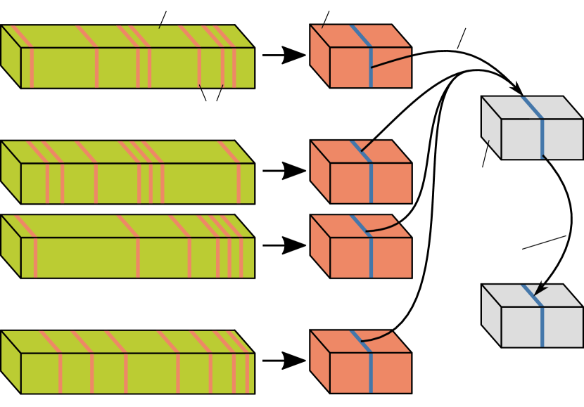
Figure 2: Illustration of how to efficiently construct $\tilde{\boldsymbol{\mathscr{G}}}^{\neq n}$ by sampling the core tensors.

Input: Samples $\bm{v}$, distributions $\{\bm{p}^{(k)}\}_{k\neq n}$

Output: Sketch $\tilde{\bm{G}}_{[2]}^{\neq n}=\bm{S}\bm{G}_{[2]}^{\neq n}$

1 Initialize $\tilde{\boldsymbol{\mathscr{G}}}^{\neq n}=\bm{0}\in\mathbb{R}^{R_{n}\times J\times R_{n-1}}$

2 for $j\in[J]$ do

     $i=\bm{v}(j)$

      // Where $i=\overline{i_{n+1}\cdots i_{N}i_{1}\cdots i_{n-1}}$

3     $c=\sqrt{J\prod_{k\neq n}\bm{p}(i_{k})}$

4     $\tilde{\boldsymbol{\mathscr{G}}}^{\neq n}(:,j,:)=\boldsymbol{\mathscr{G}}^{(n+1)}(:,i_{n+1},:)\cdots\boldsymbol{\mathscr{G}}^{(N)}(:,i_{N},:)$

5     $\;\;\;\;\;\;\;\;\;\;\;\;\;\;\;\;\;\;\;\;\cdot\boldsymbol{\mathscr{G}}^{(1)}(:,i_{1},:)\cdots\boldsymbol{\mathscr{G}}^{(n-1)}(:,i_{n-1},:)/c$

6    

7     end for

8    return $\tilde{\bm{G}}_{[2]}^{\neq n}$

Algorithm 4 Computation of $\tilde{\bm{G}}_{[2]}^{\neq n}$ (proposal)

The sampling of the data tensor on line 2 in Algorithm 2 only needs to access $JI_{n}$ entries of $\boldsymbol{\mathscr{X}}$, or less if $\boldsymbol{\mathscr{X}}$ is sparse. This is why our proposed algorithm has a cost which is sublinear in the number of entries in $\boldsymbol{\mathscr{X}}$. Due to Theorem 7, each sampled least squares solve on line 2 has high-probability relative-error guarantees, provided $J$ is large enough.

4.1 Termination Criteria

Both Algorithms 1 and 2 rely on using some termination criterion. One such criterion is to terminate the outer loop when the relative error $\|\operatorname*{\operatorname{TR}}((\boldsymbol{\mathscr{G}}^{(n)})_{n=1}^{N})-\boldsymbol{\mathscr{X}}\|_{\textup{F}}/\|\boldsymbol{\mathscr{X}}\|_{\textup{F}}$, or its change, is below some threshold. Computing the relative error exactly costs $O(I^{N}R^{2})$ which may be too costly for large tensors. In particular, it would defeat the purpose of the sublinear complexity of our method. An alternative is to terminate when the change in $\|\operatorname*{\operatorname{TR}}((\boldsymbol{\mathscr{G}}^{(n)})_{n=1}^{N})\|_{\textup{F}}$ is below some threshold. Such an approach is used for large scale Tucker decomposition by Kolda & Sun (2008) and Malik & Becker (2018). The norm $\|\operatorname*{\operatorname{TR}}((\boldsymbol{\mathscr{G}}^{(n)})_{n=1}^{N})\|_{\textup{F}}$ can be computed efficiently using an algorithm by Mickelin & Karaman (2020). When $I_{n}=I$ and $R_{n}=R$ for all $n\in[N]$ it has complexity $O(NIR^{4})$; see Section 3.3 of Mickelin & Karaman (2020). Another approach is to estimate the relative error via sampling, which is used by Battaglino et al. (2018) for their randomized CP decomposition method.

4.2 Adaptive Sample Size

Algorithm 2 can produce good results even if the sample size $J$ is smaller than what Theorem 7 suggests. Choosing an appropriate $J$ for a particular problem can therefore be challenging. Aggour et al. (2020) develop an ALS-based algorithm for CP decomposition with an adaptive sketching rate to speed up convergence. Similar ideas can easily be incorporated in our Algorithm 2. Indeed, one of the benefits of our method is that the sample size $J$ can be changed at any point with no overhead cost. By contrast, for rTR-ALS, another randomized method for TR decomposition which we describe in Section 5, the entire compression phase would need to be redone if the sketch rate is updated.

4.3 Complexity Analysis

Table 1: Comparison of leading order computational complexity. “#iter” denotes the number of outer loop iterations in the ALS-based methods.

Method	Complexity
TR-ALS	$NIR^{2}+\textup{\#iter}\cdot NI^{N}R^{2}$
rTR-ALS	$NI^{N}K+\textup{\#iter}\cdot NK^{N}R^{2}$
TR-SVD	$I^{N+1}+I^{N}R^{3}$
TR-SVD-Rand	$I^{N}R^{2}$
TR-ALS-S. (proposal)	$NIR^{4}+\textup{\#iter}\cdot\frac{NIR^{2(N+1)}}{\varepsilon\delta}$

Table 1 compares the leading order complexity of our proposed method to the four other methods we consider in the experiments. The other methods are described in Section 5. For simplicity, we assume that $I_{n}=I$ and $R_{n}=R$ for all $n\in[N]$, and that $N<I$, $R^{2}<I$ and $NR<I$. For rTR-ALS, the intermediate $N$-way Tucker core is assumed to be of size $K\times\cdots\times K$; see Yuan et al. (2019) for details. The complexity for our method in the table assumes $J$ satisfies (10), and that $\varepsilon$ and $\delta$ are small enough so that (10) simplifies to $J>4R^{2N}/(\varepsilon\delta)$. Any costs for checking convergence criteria are ignored. This is justified since e.g. the termination criterion based on computing $\|\operatorname*{\operatorname{TR}}((\boldsymbol{\mathscr{G}}^{(n)})_{n=1}^{N})\|_{\textup{F}}$ described in Section 4.1 would not impact the complexity of TR-ALS or our TR-ALS-Sampled, and would only impact that of rTR-ALS if $K^{N}<IR^{2}$. The complexities in Table 1 are derived in Section 8 of the supplement.

The complexity of our method is sublinear in the number of tensor elements, avoiding the dependence on $I^{N}$ that the other methods have. While there is still an exponential dependence on $N$, this is still much better than $I^{N}$ for low-rank decomposition of large tensors in which case $R\ll I$. This is particularly true when the input tensor is too large to store in RAM and accessing its elements dominate the cost of the decomposition. We note that our method typically works well in practice even if (10) is not satisfied.

5 Experiments

5.1 Decomposition of Real and Synthetic Datasets

We compare our proposed TR-ALS-Sampled method (Alg. 2) to four other methods: TR-ALS (Alg. 1), rTR-ALS (Alg. 1 in Yuan et al. (2019)), TR-SVD (Alg. 1 in Mickelin & Karaman (2020)) and a randomized variant of TR-SVD (Alg. 7 in Ahmadi-Asl et al. (2020)) which we refer to as TR-SVD-Rand. TR-SVD takes an error tolerance as input and makes the ranks large enough to achieve this tolerance. To facilitate comparison to the ALS-based methods, we modify TR-SVD so that it takes target ranks as inputs instead. TR-SVD-Rand takes target ranks as inputs by default. For TR-ALS, rTR-ALS and TR-SVD-Rand, we wrote our own implementations since codes were not publicly available. For TR-SVD, we modified the function TRdecomp.m provided by Mickelin & Karaman (2020). As suggested by Ahmadi-Asl et al. (2020), we use an oversampling parameter of 10 in TR-SVD-Rand. The relative error of a decomposition is computed as $\|\operatorname*{\operatorname{TR}}((\boldsymbol{\mathscr{G}}^{(n)})_{n=1}^{N})-\boldsymbol{\mathscr{X}}\|_{\textup{F}}/\|\boldsymbol{\mathscr{X}}\|_{\textup{F}}$.

To get a fair comparison between the different methods we first decompose the input tensor with TR-ALS by running it until a convergence criterion has been met or a maximum number of iterations reached. All ALS-based algorithms (including TR-ALS) are then applied to the input tensor, running for twice as many iterations as it took the initial TR-ALS run to terminate, without checking any convergence criteria. This is done to strip away any run time influence that checking convergence has and only compare those aspects that differ between the methods. TR-ALS-Sampled and rTR-ALS apply sketching in fundamentally different ways. To best understand the trade-off between run time and accuracy, we start out these two algorithm with small sketch rates ($J$ and $K$, respectively) and increase them until the resulting relative error is less than $(1+\varepsilon)E$, where $E$ is the relative error achieved by TR-ALS during the second run and $\varepsilon\in(0,1)$. The relative error and run time for the smallest sketch rate that achieve this relative-error bound are then reported. The exact details on how this is done for each individual experiment is described in Section 10 of the supplement.

All experiments are run in Matlab R2017a with Tensor Toolbox 2.6 (Bader et al., 2015) on a computer with an Intel Xeon E5-2630 v3 @ 32x 3.2GHz CPU and 32 GB of RAM. All our code used in the experiments is available online.

5.1.1 Randomly Generated Data

Synthetic 3-way tensors are generated by creating 3 cores of size $R^{\prime}\times I\times R^{\prime}$ with entries drawn independently from a standard normal distribution. Here, $R^{\prime}$ is used to denote true rank, as opposed to the rank $R$ used in the decomposition. For each core, one entry is chosen uniformly at random and set to 20. The goal of this is to increase the coherence in the least squares problems, which makes them more challenging for sampling-based methods like ours. The cores are then combined into a full tensor via (1). Finally, Gaussian noise with standard deviation 0.1 is added to all entries in the tensor independently.

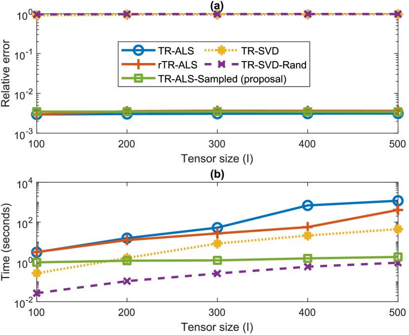
Figure 3: Synthetic experiment with true and target ranks $R^{\prime}=R=10$. (a) Relative error and (b) run time for each of the five methods. Average number of ALS iterations used is 21.

In the first synthetic experiment $R^{\prime}=10$ and $I\in\{100,200,\ldots,500\}$. The target rank is also set to $R=10$. Ideally, decompositions should therefore have low error. Figure 3 shows the relative error and run time for the five different algorithms. All plotted quantities are the median over 10 runs. The ALS-based algorithms reach very low errors. On average, only 21 iterations are needed, and the number of iterations is fairly stable when the tensor size is increased. The SVD-based algorithms, by contrast do very poorly, having relative errors close to 1. Our proposed TR-ALS-Sampled is the fastest method, aside from TR-SVD-Rand which returns very poor results. We achieve a substantial speedup of $668\times$ over TR-ALS and $230\times$ over rTR-ALS for $I=500$.

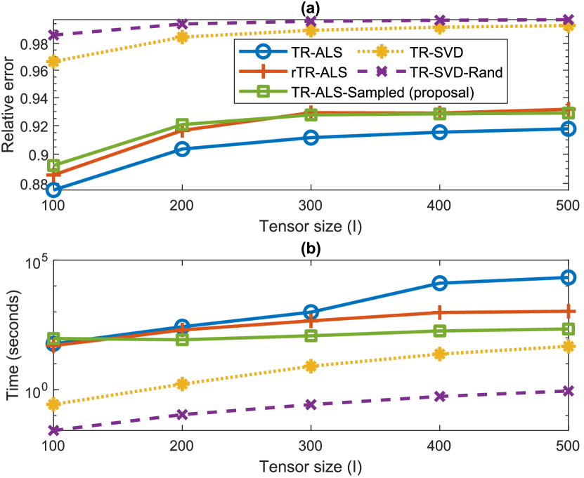
Figure 4: Synthetic experiment with true rank $R^{\prime}=20$ and target rank $R=10$. (a) Relative error and (b) run time for each of the five methods. Average number of ALS iterations used is 417.

In the second synthetic experiment, we set $R^{\prime}=20$ but keep the target rank at $R=10$. We therefore expect the decompositions to have a larger relative error. Figure 4 shows the results for these experiments. All plotted quantities are the median over 10 runs. The ALS-based methods still outperform the SVD-based ones. The ALS-based methods now require more iterations, on average running for 417 iterations, with greater variability between runs. Our proposed TR-ALS-Sampled remains faster than the other ALS-based methods, although with a smaller difference, achieving a speedup of $98\times$ over TR-ALS and $5\times$ over rTR-ALS for $I=500$. Although the SVD-based methods are faster, especially the randomized variant, they are not useful since they give such a high error. See Remarks 16 and 17 in the supplement for further discussion of the results in Figures 3 and 4.

The signal-to-noise ratio (SNR) is about 50 dB and 59 dB, respectively, in the two experiments above. To validate the robustness of those results to higher levels of noise we run additional experiments on synthetic $300\times 300\times 300$ tensors with added Gaussian noise with standard deviation 1 and 10 which corresponds to an SNR of 30 dB and 10 dB, respectively. All other settings are kept the same as in the first synthetic experiment. The results, shown in Figure 5, indicate that the earlier experiment results are robust to higher noise levels.

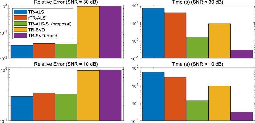
Figure 5: Comparison of methods for higher levels of noise.

5.1.2 Highly Oscillatory Functions

Table 2: Decomposition results for highly oscillatory functions with target rank $R=10$.

	Linear Growth		Airy		Chirp
Method	Error	Time (s)	Error	Time (s)	Error	Time (s)
TR-ALS	$0.0102$	$370.3$	$0.0203$	$531.7$	$0.0198$	$613.1$
rTR-ALS	$0.0105$	$382.8$	$0.0186$	$521.6$	$0.0193$	$645.9$
TR-ALS-Sampled (proposal)	$0.0109$	$3.4$	$0.0213$	$2.7$	$0.0210$	$36.2$

Next, we decompose the highly oscillatory functions considered by Zhao et al. (2016). The functions are illustrate in Figure 6. Each function is evaluated at $4^{10}$ points. These values are then reshaped into 10-way tensors of size $4\times\cdots\times 4$ which are then decomposed. Table 2 shows the results for when all target ranks are $R=10$. The SVD-based methods can not be applied in this experiment since they require $R_{0}R_{1}\leq I_{1}$ which is not satisfied.

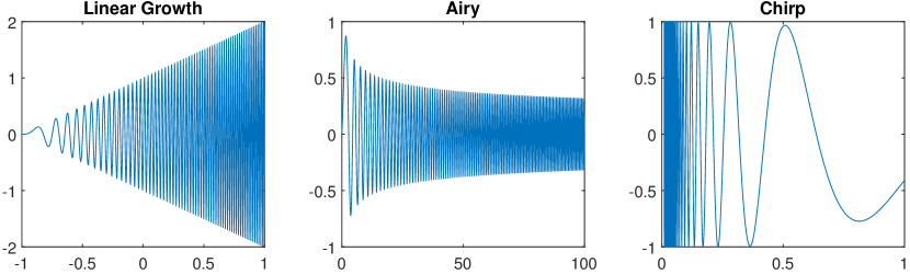
Figure 6: The functions are defined as follows. Linear growth: $(x+1)\sin(100(x+1)^{2})$. Airy: $x^{-1/4}\sin(2x^{3/2}/3)$. Chirp: $\sin(4/x)\cos(x^{2})$.

All algorithms achieve a relative error of only 1%–2%. This is impressive, especially considering that the choice of $R_{n}=10$ correspond to a $262\times$ compression rate. With an error very similar to that of TR-ALS, our proposal TR-ALS-Sampled achieves speedups of $108\times$, $193\times$ and $17\times$ on the three tensors over TR-ALS. Our method achieves speedups of $112\times$, $190\times$ and $18\times$ over rTR-ALS. Notice that rTR-ALS yields no speedup over TR-ALS in Table 2. The reason for this is that each $I_{n}=4$ is so small. For rTR-ALS to have acceptable accuracy, $K$ must be chosen to be $K=4$, meaning that rTR-ALS is just as slow as TR-ALS.

5.1.3 Image and Video Data

We consider five real image and video datasets (sizes in parentheses): Pavia University ($610\times 340\times 103$) and DC Mall ($1280\times 307\times 191$) are 3-way tensors containing hyperspectral images. The first two dimensions are the image height and width, and the third dimension is the number of spectral bands. Park Bench ($1080\times 1920\times 364$) and Tabby Cat ($720\times 1280\times 286$) are 3-way tensors representing grayscale videos of a man sitting on a park bench and a cat, respectively. The first two dimension are frame height and width, and the third dimension is the number of frames. Red Truck ($128\times 128\times 3\times 72$) is a 4-way tensor consisting of 72 color images of size 128 by 128 pixels depicting a red truck from different angles. It is a subset of the COIL-100 dataset (Nene et al., 1996).

Tables 3 and 4 show results for when all target ranks are $R=10$ and $R=20$, respectively. The SVD-based algorithms require $R_{0}R_{1}\leq I_{1}$, so they cannot handle the Red Truck tensor when $R=20$ since $I_{1}=128$ for that dataset. All results are based on a single trial. Our proposed TR-ALS-Sampled runs faster than the other ALS-based methods on all image and video datasets, achieving up to $1518\times$ speedup over TR-ALS (for the Park Bench tensor with $R=10$) and a $21\times$ speedup over rTR-ALS (for the Red Truck tensor with $R=20$). The SVD-based methods perform better than they did on the randomly generated data, but remain worse than the ALS-based methods. TR-SVD-Rand is always the fastest method, but also has a substantially higher error.

Table 3: Decomposition results for real datasets with target rank $R=10$. Time is in seconds.

	Pavia Uni.		DC Mall		Park Bench		Tabby Cat		Red Truck
Method	Error	Time	Error	Time	Error	Time	Error	Time	Error	Time
TR-ALS	$0.1639$	$62.075$	$0.159\,81$	$801.4$	$0.073\,525$	$5384.9$	$0.135\,79$	$1769.4$	$0.1765$	$181.21$
rTR-ALS	$0.175\,66$	$16.251$	$0.173\,46$	$25.37$	$0.080\,53$	$64.814$	$0.144\,47$	$8.9931$	$0.193\,07$	$21.984$
TR-ALS-S. (proposal)	$0.177\,55$	$1.727$	$0.1754$	$3.0827$	$0.080\,136$	$3.5475$	$0.147\,86$	$2.4187$	$0.190\,77$	$1.9332$
TR-SVD	$0.2121$	$2.138$	$0.204\,15$	$12.773$	$0.078\,14$	$136.45$	$0.153\,59$	$37.73$	$0.262\,19$	$1.2844$
TR-SVD-Rand	$0.326\,51$	$0.162\,43$	$0.297\,38$	$0.335\,25$	$0.110\,89$	$2.7777$	$0.196\,14$	$1.5828$	$0.292\,76$	$0.085\,354$

Table 4: Decomposition results for real datasets with target rank $R=20$. The ✗ signifies that the SVD-based methods cannot handle this case since they require $R_{0}R_{1}\leq I_{1}$. Time is in seconds.

	Pavia Uni.		DC Mall		Park Bench		Tabby Cat		Red Truck
Method	Error	Time	Error	Time	Error	Time	Error	Time	Error	Time
TR-ALS	$0.061\,195$	$249.91$	$0.057\,176$	$622.81$	$0.041\,872$	$2385.0$	$0.108\,38$	$1397.2$	$0.110\,19$	$1279.1$
rTR-ALS	$0.066\,827$	$194.61$	$0.062\,014$	$349.63$	$0.045\,118$	$531.46$	$0.115\,64$	$92.591$	$0.118\,64$	$470.59$
TR-ALS-S. (proposal)	$0.066\,52$	$13.738$	$0.062\,687$	$26.535$	$0.045\,891$	$24.952$	$0.119\,09$	$19.0$	$0.119\,58$	$22.607$
TR-SVD	$0.098\,693$	$4.587$	$0.102\,65$	$25.401$	$0.048\,204$	$271.99$	$0.130\,57$	$110.0$	✗	✗
TR-SVD-Rand	$0.281\,56$	$0.500\,99$	$0.252\,83$	$1.0098$	$0.098\,901$	$8.5071$	$0.168\,21$	$4.0938$	✗	✗

A popular preprocessing step used in tensor decomposition is to first reshape a tensor into a tensor with more modes. Next, we therefore try reshaping the five tensors above so that they each have twice as many modes. Some of the dimensions are truncated slightly to allow for this reshaping. Our method yields speedups in the range $94\times$–$2880\times$ over TR-ALS and $73\times$–$1484\times$ over rTR-ALS. The SVD-based methods cannot be applied since they require $R_{0}R_{1}\leq I_{1}$ which is not satisfied for these reshaped tensors. The speed benefit of our method appears to be even greater when increasing the number of modes. Please see Section 10.3 of the supplement for further details on this experiment, including detailed results.

An alternative to sampling according to the distribution defined by the leverage scores in (7) and (8) is to simply sample according to the uniform distribution, i.e., $\bm{q}^{\neq n}=1/\prod_{j\neq n}I_{j}$. Although such a sampling approach does not come with any guarantees, it is faster than leverage score sampling since it avoids the cost of computing the sampling distribution. In order to investigate the performance of uniform sampling, we repeat the experiments whose results are show in Tables 3 and 4 for TR-ALS-Sampled, but using uniform sampling instead of leverage score sampling. Everything else is kept the same. Table 5 shows the results.

Table 5: Decomposition results for TR-ALS-Sampled with uniform sampling.

	$R=10$		$R=20$
Dataset	Error	Time (s)	Error	Time (s)
Pavia Uni.	0.18	1.3	0.07	9.0
DC Mall	0.18	3.7	0.06	22.2
Park Bench	0.08	5.8	0.05	28.0
Tabby Cat	0.15	2.2	0.12	23.1
Red Truck	0.20	1.5	0.12	18.7

Using uniform instead of leverage score sampling does not appear to impact the error and overall run time much. However, uniform sampling requires 4.6–8.8 times as many samples to reach the target accuracy. Although more samples increase the cost of the least squares solve, the cost of updating the sampling distribution is avoided. It may be possible to combine uniform and leverage score sampling to speed up our method while still retaining some guarantees. Uniform sampling has also yielded promising empirical results for the CP decomposition; see e.g. Battaglino et al. (2018) and Aggour et al. (2020).

5.2 Rapid Feature Extraction for Classification

Inspired by experiments in Zhao et al. (2016), we now give a practical example of how our method can be used for rapid feature extraction for classification. We consider the full COIL-100 dataset which consists of 7200 color images of size $128\times 128$ depicting 100 different objects from 72 different angles each. The images are downsampled to $32\times 32$ and stacked into a tensor $\boldsymbol{\mathscr{X}}$ of size $32\times 32\times 3\times 7200$. We then use the various TR decomposition algorithms to compute a TR decomposition of $\boldsymbol{\mathscr{X}}$ with each rank $R_{n}=5$. Additional details on algorithm settings are given in Section 10.4 of the supplement. The TR core $\boldsymbol{\mathscr{G}}^{(4)}$ is of size $5\times 7200\times 5$ and contains latent features for the 4th mode of $\boldsymbol{\mathscr{X}}$. We reshape it into a $7200\times 25$ feature matrix and apply the $k$-nearest neighbor algorithm with $k=1$. Table 6 reports the decomposition error as well as the accuracy achieved when classifying the 7200 images into the 100 different classes. The classification is done using 10-fold cross validation. The ALS-based methods yield a lower error than the SVD-based methods. All methods result in a similar classification accuracy. The higher decomposition errors for the SVD-based methods do not seem to compromise classification accuracy.

Table 6: Decomposition error and classification accuracy for rapid feature extraction experiment.

Method	Time (s)	Error	Acc. (%)
TR-ALS	248.7	0.27	99.07
rTR-ALS	3.1	0.29	98.96
TR-ALS-S. (proposal)	12.7	0.28	99.32
TR-SVD	7.3	0.37	99.68
TR-SVD-Rand	0.7	0.33	99.85

6 Conclusion

We have proposed a method for TR decomposition which uses leverage score sampled ALS and has complexity sublinear in the number of input tensor entries. We also proved high-probability relative-error guarantees for the sampled least squares problems. Our method achieved substantial speedup over competing methods in experiments on both synthetic and real data, in some cases by as much as two or three orders of magnitude, while maintaining good accuracy. We also demonstrated how our method can be used for rapid feature extraction.

The datasets in our experiments are dense. Based on limited testing, rTR-ALS seems to do particularly well on sparse datasets, outperforming our proposed method. Our method still yielded a substantial speedup over TR-ALS. Further investigating this, and optimizing the various methods for sparse tensors, is an interesting direction for future research.

7 Missing Proofs

In this section we give proofs for Lemma 6 and Theorem 7 in the main manuscript. We first state some results that we will use in these proofs.

Lemma 8 is a variant of Lemma 1 by Drineas et al. (2011) but for multiple right hand sides. The proof by Drineas et al. (2011) remains essentially identical with only minor modifications to account for the multiple right hand sides.

Lemma 8.

Let $\textup{OPT}\stackrel{{\scriptstyle\text{\tiny{def}}}}{{=}}\min_{\bm{X}}\|\bm{A}\bm{X}-\bm{Y}\|_{\textup{F}}$ be a least squares problem where $\bm{A}\in\mathbb{R}^{I\times R}$ and $I>R$, and let $\bm{U}\in\mathbb{R}^{I\times\operatorname{rank}(\bm{A})}$ contain the left singular vectors of $\bm{A}$. Moreover, let $\bm{U}^{\perp}$ be an orthogonal matrix whose columns span the space perpendicular to $\operatorname{range}(\bm{U})$ and define $\bm{Y}^{\perp}\stackrel{{\scriptstyle\text{\tiny{def}}}}{{=}}\bm{U}^{\perp}(\bm{U}^{\perp})^{\top}\bm{Y}$. Let $\bm{S}\in\mathbb{R}^{J\times I}$ be a matrix satisfying

$$\sigma^{2}_{\min}(\bm{S}\bm{U})\geq\frac{1}{\sqrt{2}},$$ (13)

$$\|\bm{U}^{\top}\bm{S}^{\top}\bm{S}\bm{Y}^{\perp}\|_{\textup{F}}^{2}\leq\frac{\varepsilon}{2}\textup{OPT}^{2},$$ (14)

for some $\varepsilon\in(0,1)$. Then, it follows that

$$\|\bm{A}\tilde{\bm{X}}-\bm{Y}\|_{\textup{F}}\leq(1+\varepsilon)\textup{OPT},$$ (15)

where $\tilde{\bm{X}}\stackrel{{\scriptstyle\text{\tiny{def}}}}{{=}}\operatorname*{arg\,min}_{\bm{X}}\|\bm{S}\bm{A}\bm{X}-\bm{S}\bm{Y}\|_{\textup{F}}$.

Lemma 9 is a slight restatement of Theorem 2.11 in the monograph by Woodruff (2014). The statement in that monograph has a constant $144$ instead of $8/3$. However, we found that $8/3$ is sufficient under the assumption that $\varepsilon\in(0,1)$. The proof given by Woodruff (2014) otherwise remains the same.

Lemma 9.

Let $\bm{A}\in\mathbb{R}^{I\times R}$, $\varepsilon\in(0,1)$, $\eta\in(0,1)$ and $\beta\in(0,1]$. Suppose

$$J>\frac{8}{3}\frac{R\ln(2R/\eta)}{\beta\varepsilon^{2}}$$ (16)

and that $\bm{S}\sim\mathcal{D}(J,\bm{q})$ is a leverage score sampling matrix for $(\bm{A},\beta)$ (see Definition 5 in the main manuscript). Then, with probability at least $1-\eta$, the following holds:

$$(\forall i\in[\operatorname{rank}(\bm{A})])\;\;\;\;1-\varepsilon\leq\sigma_{i}^{2}(\bm{S}\bm{U})\leq 1+\varepsilon,$$ (17)

where $\bm{U}\in\mathbb{R}^{I\times\operatorname{rank}(\bm{A})}$ contains the left singular vectors of $\bm{A}$.

Lemma 10 is a part of Lemma 8 by Drineas et al. (2006).

Lemma 10.

Let $\bm{A}$ and $\bm{B}$ be matrices with $I$ rows, and let $\beta\in(0,1]$. Let $\bm{q}\in\mathbb{R}^{I}$ be a probability distribution satisfying

$$\bm{q}(i)\geq\beta\frac{\|\bm{A}(i,:)\|^{2}_{2}}{\|\bm{A}\|_{\textup{F}}^{2}}\;\;\;\;\text{for all }i\in[I].$$ (18)

If $\bm{S}\sim\mathcal{D}(J,\bm{q})$, then

$$\mathbb{E}\|\bm{A}^{\top}\bm{B}-\bm{A}^{\top}\bm{S}^{\top}\bm{S}\bm{B}\|_{\textup{F}}^{2}\leq\frac{1}{\beta J}\|\bm{A}\|_{\textup{F}}^{2}\|\bm{B}\|_{\textup{F}}^{2}.$$ (19)

In the following, $\otimes$ denotes the matrix Kronecker product; see e.g. Section 1.3.6 of Golub & Van Loan (2013) for details.

Lemma 11.

For $n\in[N]$, the subchain $\boldsymbol{\mathscr{G}}^{\neq n}$ satisfies

$$\operatorname{range}(\bm{G}_{[2]}^{\neq n})\subseteq\operatorname{range}(\bm{G}_{(2)}^{(n-1)}\otimes\cdots\otimes\bm{G}_{(2)}^{(1)}\otimes\bm{G}_{(2)}^{(N)}\otimes\cdots\otimes\bm{G}_{(2)}^{(n+1)}).$$ (20)

Proof.

We have

$$\bm{G}_{[2]}^{\neq n}(\overline{i_{n+1}\cdots i_{N}i_{1}\cdots i_{n-1}},\overline{r_{n-1}r_{n}})=$$ (21)

$$\sum_{\begin{subarray}{c}r_{1},\ldots,r_{n-2}\\ r_{n+1},\ldots,r_{N}\end{subarray}}\bm{G}_{(2)}^{(n+1)}(i_{n+1},\overline{r_{n}r_{n+1}})\cdots\bm{G}_{(2)}^{(N)}(i_{N},\overline{r_{N-1}r_{N}})\bm{G}_{(2)}^{(1)}(i_{1},\overline{r_{N}r_{1}})\cdots\bm{G}_{(2)}^{(n-1)}(i_{n-1},\overline{r_{n-2}r_{n-1}}).$$

From this, it follows that

$$\bm{G}_{[2]}^{\neq n}(:,\overline{r_{n-1}r_{n}})=$$ (22)

$$\sum_{\begin{subarray}{c}r_{1},\ldots,r_{n-2}\\ r_{n+1},\ldots,r_{N}\end{subarray}}\bm{G}_{(2)}^{(n-1)}(:,\overline{r_{n-2}r_{n-1}})\otimes\cdots\otimes\bm{G}_{(2)}^{(1)}(:,\overline{r_{N}r_{1}})\otimes\bm{G}_{(2)}^{(N)}(:,\overline{r_{N-1}r_{N}})\otimes\cdots\otimes\bm{G}_{(2)}^{(n+1)}(:,\overline{r_{n}r_{n+1}}).$$

The right hand side of this equation is a sum of columns in

$$\bm{G}_{(2)}^{(n-1)}\otimes\cdots\otimes\bm{G}_{(2)}^{(1)}\otimes\bm{G}_{(2)}^{(N)}\otimes\cdots\otimes\bm{G}_{(2)}^{(n+1)}.$$ (23)

Consequently, every column of $\bm{G}_{[2]}^{\neq n}$ is in the range of the matrix in (23), and the claim in (20) follows. ∎

Lemma 12.

Let $\bm{A}$ and $\bm{B}$ be two matrices with $I$ rows such that $\operatorname{range}(\bm{A})\subseteq\operatorname{range}(\bm{B})$. Then $\ell_{i}(\bm{A})\leq\ell_{i}(\bm{B})$ for all $i\in[I]$.

Proof.

Let $\bm{Q}\in\mathbb{R}^{I\times\operatorname{rank}(\bm{B})}$ be an orthogonal matrix containing the left singular vectors of $\bm{B}$. Then there exists a matrix $\bm{M}$ such that $\bm{A}=\bm{Q}\bm{M}$. Let $\bm{U}\bm{\Sigma}\bm{V}^{\top}=\bm{M}$ be the thin SVD of $\bm{M}$ (i.e., such that $\bm{U}$ and $\bm{V}$ have only $\operatorname{rank}(\bm{M})$ columns and $\bm{\Sigma}\in\mathbb{R}^{\operatorname{rank}(\bm{M})\times\operatorname{rank}(\bm{M})}$). Then $\bm{A}=\bm{Q}\bm{U}\bm{\Sigma}\bm{V}^{\top}=\bm{W}\bm{\Sigma}\bm{V}^{\top}$, where $\bm{W}\stackrel{{\scriptstyle\text{\tiny{def}}}}{{=}}\bm{Q}\bm{U}$. Since

$$\bm{W}^{\top}\bm{W}=\bm{U}^{\top}\bm{Q}^{\top}\bm{Q}\bm{U}=\bm{I},$$ (24)

$\bm{W}$ is orthogonal, so $\bm{W}\bm{\Sigma}\bm{V}^{\top}=\bm{A}$ is a thin SVD of $\bm{A}$. It follows that

$$\ell_{i}(\bm{A})=\|\bm{W}(i,:)\|_{2}^{2}=\|\bm{Q}(i,:)\bm{U}\|_{2}^{2}\leq\|\bm{Q}(i,:)\|_{2}^{2}\|\bm{U}\|^{2}_{2}=\|\bm{Q}(i,:)\|_{2}^{2}=\ell_{i}(\bm{B}).$$ (25)

∎

Remark 13.

It is reasonable to assume that $\boldsymbol{\mathscr{G}}^{\neq n}\neq\bm{0}$ for all $n\in[N]$ during the execution of Algorithms 1 and 2. If this was not the case, the least squares problem for the $n$th iteration of the inner for loop in these algorithms would have a zero system matrix which would make the least squares problem meaningless. The assumption $\boldsymbol{\mathscr{G}}^{\neq n}\neq\bm{0}$ for all $n\in[N]$ also implies that $\boldsymbol{\mathscr{G}}^{(n)}\neq\bm{0}$ for all $n\in[N]$. This means that $\operatorname{rank}(\bm{G}_{(2)}^{(n)})\geq 1$ and $\operatorname{rank}(\bm{G}_{[2]}^{\neq n})\geq 1$ for all $n\in[N]$, so that the various divisions with these quantities in this paper are well-defined.

Lemma 14 is a restatement of Lemma 6 in the main manuscript.

Lemma 14.

Let $\beta_{n}$ be defined as

$$\beta_{n}\stackrel{{\scriptstyle\text{\tiny{def}}}}{{=}}\Big{(}R_{n-1}R_{n}\prod_{\begin{subarray}{c}j=1\\ j\notin\{n-1,n\}\end{subarray}}^{N}R_{j}^{2}\Big{)}^{-1}.$$ (26)

For each $n\in[N]$, the vector $\bm{q}^{\neq n}$ is a probability distribution on $[\prod_{j\neq n}I_{j}]$, and $\bm{S}\sim\mathcal{D}(J,\bm{q}^{\neq n})$ is a leverage score sampling matrix for $(\bm{G}_{[2]}^{\neq n},\beta_{n})$.

Proof.

All $\bm{q}^{\neq n}(i)$ are clearly nonnegative. Moreover,

$$\sum_{\begin{subarray}{c}i_{1},\ldots,i_{n-1}\\ i_{n+1},\ldots,i_{N}\end{subarray}}\bm{q}^{\neq n}(\overline{i_{n+1}\cdots i_{N}i_{1}\cdots i_{n-1}})=\prod_{\begin{subarray}{c}j=1\\ j\neq n\end{subarray}}^{N}\sum_{i_{j}}\bm{p}^{(j)}(i_{j})=\prod_{\begin{subarray}{c}j=1\\ j\neq n\end{subarray}}^{N}1=1,$$ (27)

since each $\bm{p}^{(j)}$ is a probability distribution. So $\bm{q}^{\neq n}$ is clearly also a probability distribution. Next, define the vector $\bm{p}\in\mathbb{R}^{\prod_{j\neq n}I_{n}}$ via

$$\bm{p}(i)\stackrel{{\scriptstyle\text{\tiny{def}}}}{{=}}\frac{\ell_{i}(\bm{G}_{[2]}^{\neq n})}{\operatorname{rank}(\bm{G}_{[2]}^{\neq n})}.$$ (28)

To show that $\bm{S}$ is a leverage score sampling matrix for $(\bm{G}_{[2]}^{\neq n},\beta_{n})$, we need to show that $\bm{q}^{\neq n}(i)\geq\beta_{n}\bm{p}(i)$ for all $i=\overline{i_{n+1}\cdots i_{N}i_{1}\cdots i_{n-1}}\in[\prod_{j\neq n}I_{n}]$. To this end, combine Lemmas 11 and 12 to get

$$\ell_{i}(\bm{G}_{[2]}^{\neq n})\leq\ell_{i}(\bm{G}_{(2)}^{(n-1)}\otimes\cdots\otimes\bm{G}_{(2)}^{(1)}\otimes\bm{G}_{(2)}^{(N)}\otimes\cdots\otimes\bm{G}_{(2)}^{(n+1)}).$$ (29)

For each $n\in[N]$, let $\bm{U}^{(n)}\in\mathbb{R}^{I_{n}\times\operatorname{rank}(\bm{G}_{(2)}^{(n)})}$ contain the left singular vectors of $\bm{G}_{(2)}^{(n)}$. It is well-known (Van Loan, 2000) that the matrix

$$\bm{U}^{(n-1)}\otimes\cdots\otimes\bm{U}^{(1)}\otimes\bm{U}^{(N)}\otimes\cdots\otimes\bm{U}^{(n+1)}$$ (30)

contains the left singular vectors corresponding to nonzero singular values of

$$\bm{G}_{(2)}^{(n-1)}\otimes\cdots\otimes\bm{G}_{(2)}^{(1)}\otimes\bm{G}_{(2)}^{(N)}\otimes\cdots\otimes\bm{G}_{(2)}^{(n+1)}.$$ (31)

Consequently,

$$\ell_{i}(\bm{G}_{(2)}^{(n-1)}\otimes\cdots\otimes\bm{G}_{(2)}^{(1)}\otimes\bm{G}_{(2)}^{(N)}\otimes\cdots\otimes\bm{G}_{(2)}^{(n+1)})$$ (32)

$$=\big{(}(\bm{U}^{(n-1)}\otimes\cdots\otimes\bm{U}^{(1)}\otimes\bm{U}^{(N)}\otimes\cdots\otimes\bm{U}^{(n+1)})(\bm{U}^{(n-1)}\otimes\cdots\otimes\bm{U}^{(1)}\otimes\bm{U}^{(N)}\otimes\cdots\otimes\bm{U}^{(n+1)})^{\top}\big{)}_{ii}$$

$$=\big{(}(\bm{U}^{(n-1)}\bm{U}^{(n-1)\top})\otimes\cdots\otimes(\bm{U}^{(1)}\bm{U}^{(1)\top})\otimes(\bm{U}^{(N)}\bm{U}^{(N)\top})\otimes\cdots\otimes(\bm{U}^{(n+1)}\bm{U}^{(n+1)\top})\big{)}_{ii}$$

$$=(\bm{U}^{(n-1)}\bm{U}^{(n-1)\top})_{i_{n-1}i_{n-1}}\cdots(\bm{U}^{(1)}\bm{U}^{(1)\top})_{i_{1}i_{1}}(\bm{U}^{(N)}\bm{U}^{(N)\top})_{i_{N}i_{N}}\cdots(\bm{U}^{(n+1)}\bm{U}^{(n+1)\top})_{i_{n+1}i_{n+1}}$$

$$=\ell_{i_{n-1}}(\bm{G}_{(2)}^{(n-1)})\cdots\ell_{i_{1}}(\bm{G}_{(2)}^{(1)})\ell_{i_{N}}(\bm{G}_{(2)}^{(N)})\cdots\ell_{i_{n+1}}(\bm{G}_{(2)}^{(n+1)}),$$

where the first and fourth equalities follow from the definition of leverage score and the fact that

$$\|\bm{M}(i,:)\|_{2}^{2}=(\bm{M}\bm{M}^{\top})(i,i)$$ (33)

for any matrix $\bm{M}$, and the second equality follows from well-known properties of the Kronecker product (Van Loan, 2000). Combining (29) and (32), we have

$$\ell_{i}(\bm{G}_{[2]}^{\neq n})\leq\prod_{\begin{subarray}{c}j=1\\ j\neq n\end{subarray}}^{N}\ell_{i_{j}}(\bm{G}_{(2)}^{(j)}).$$ (34)

We therefore have

$$\bm{q}^{\neq n}(i)=\frac{\prod_{j\neq n}\ell_{i_{j}}(\bm{G}_{(2)}^{(j)})}{\prod_{j\neq n}\operatorname{rank}(\bm{G}_{(2)}^{(j)})}\geq\frac{\ell_{i}(\bm{G}_{[2]}^{\neq n})}{R_{n-1}R_{n}\prod_{j\in[N]\setminus\{n-1,n\}}R_{j}^{2}}=\beta_{n}\ell_{i}(\bm{G}_{[2]}^{\neq n})\geq\beta_{n}\bm{p}(i)$$ (35)

as desired, where the first inequality follows from (34) and the fact that $\operatorname{rank}(\bm{G}_{(2)}^{(j)})\leq R_{j-1}R_{j}$. ∎

The following is a restatement of Theorem 7 in the main manuscript. The proof is similar to that of Theorem 2 by Drineas et al. (2011).

Theorem 15.

Let $\bm{S}\sim\mathcal{D}(J,\bm{q}^{\neq n})$, $\varepsilon\in(0,1)$, $\delta\in(0,1)$ and $\tilde{\boldsymbol{\mathscr{Z}}}\stackrel{{\scriptstyle\text{\tiny{def}}}}{{=}}\operatorname*{arg\,min}_{\boldsymbol{\mathscr{Z}}}\|\bm{S}\bm{G}_{[2]}^{\neq n}\bm{Z}_{(2)}^{\top}-\bm{S}\bm{X}_{[n]}^{\top}\|_{\textup{F}}$. If

$$J>\Big{(}\prod_{j=1}^{N}R_{j}^{2}\Big{)}\max\Big{(}\frac{16}{3(\sqrt{2}-1)^{2}}\ln\Big{(}\frac{4R_{n-1}R_{n}}{\delta}\Big{)},\frac{4}{\varepsilon\delta}\Big{)},$$ (36)

then the following holds with probability at least $1-\delta$:

$$\|\bm{G}_{[2]}^{\neq n}\tilde{\bm{Z}}_{(2)}^{\top}-\bm{X}_{[n]}^{\top}\|_{\textup{F}}\leq(1+\varepsilon)\min_{\boldsymbol{\mathscr{Z}}}\|\bm{G}_{[2]}^{\neq n}\bm{Z}_{(2)}^{\top}-\bm{X}_{[n]}^{\top}\|_{\textup{F}}.$$ (37)

Proof.

Let $\bm{U}\in\mathbb{R}^{\prod_{j\neq n}I_{j}\times\operatorname{rank}(\bm{G}_{[2]}^{\neq n})}$ contain the left singular vectors of $\bm{G}_{[2]}^{\neq n}$. According to Lemma 14, $\bm{S}$ is a leverage score sampling matrix for $(\bm{G}_{[2]}^{\neq n},\beta_{n})$. Since $\bm{U}$ has at most $R_{n-1}R_{n}$ columns and

$$J>\frac{16}{3(\sqrt{2}-1)^{2}}\Big{(}\prod_{j=1}^{N}R_{j}^{2}\Big{)}\ln\Big{(}\frac{4R_{n-1}R_{n}}{\delta}\Big{)},$$ (38)

choosing $\varepsilon=1-1/\sqrt{2}$ and $\eta=\delta/2$ in Lemma 9 therefore gives that

$$\sigma_{\min}^{2}(\bm{S}\bm{U})\geq 1/\sqrt{2}$$ (39)

with probability at least $1-\delta/2$. Similarly to Lemma 8, define $(\bm{X}_{[n]}^{\top})^{\perp}\stackrel{{\scriptstyle\text{\tiny{def}}}}{{=}}\bm{U}^{\perp}(\bm{U}^{\perp})^{\top}\bm{X}_{[n]}^{\top}$ and $\textup{OPT}\stackrel{{\scriptstyle\text{\tiny{def}}}}{{=}}\min_{\boldsymbol{\mathscr{Z}}}\|\bm{G}_{[2]}^{\neq n}\bm{Z}_{(2)}^{\top}-\bm{X}_{[n]}^{\top}\|_{\textup{F}}=\|(\bm{X}_{[n]}^{\top})^{\perp}\|_{\textup{F}}$. Since

$$\bm{q}^{\neq n}(i)\geq\beta_{n}\frac{\ell_{i}(\bm{G}_{[2]}^{\neq n})}{\operatorname{rank}(\bm{G}_{[2]}^{\neq n})}=\beta_{n}\frac{\|\bm{U}(i,:)\|_{2}^{2}}{\|\bm{U}\|_{\textup{F}}^{2}}\;\;\;\;\text{for all }i\in[I],$$ (40)

and $\bm{U}^{\top}(\bm{X}_{[n]}^{\top})^{\perp}=\bm{0}$, Lemma 10 gives that

$$\mathbb{E}\|\bm{U}^{\top}\bm{S}^{\top}\bm{S}(\bm{X}_{[n]}^{\top})^{\perp}\|_{\textup{F}}^{2}\leq\frac{1}{\beta_{n}J}\|\bm{U}\|_{\textup{F}}^{2}\|(\bm{X}_{[n]}^{\top})^{\perp}\|_{\textup{F}}^{2}\leq\frac{R_{n-1}R_{n}}{\beta_{n}J}\textup{OPT}^{2}.$$ (41)

By Markov’s inequality,

$$\mathbb{P}(\|\bm{U}^{\top}\bm{S}^{\top}\bm{S}(\bm{X}_{[n]}^{\top})^{\perp}\|_{\textup{F}}^{2}>\varepsilon\textup{OPT}^{2}/2)\leq\frac{\mathbb{E}\|\bm{U}^{\top}\bm{S}^{\top}\bm{S}(\bm{X}_{[n]}^{\top})^{\perp}\|_{\textup{F}}^{2}}{\varepsilon\textup{OPT}^{2}/2}\leq\frac{2}{\varepsilon J}\Big{(}\prod_{j\in[N]}R_{j}^{2}\Big{)}<\frac{\delta}{2}$$ (42)

since

$$J>\frac{4}{\varepsilon\delta}\Big{(}\prod_{j=1}^{N}R_{j}^{2}\Big{)}.$$ (43)

Consequently,

$$\|\bm{U}^{\top}\bm{S}^{\top}\bm{S}(\bm{X}_{[n]}^{\top})^{\perp}\|_{\textup{F}}^{2}\leq\frac{\varepsilon}{2}\textup{OPT}^{2}$$ (44)

with probability at least $1-\delta/2$. By a union bound, it follows that both (39) and (44) are true with probability at least $1-\delta$. From Lemma 8 it therefore follows that (37) is true with probability at least $1-\delta$. ∎

8 Detailed Complexity Analysis

We provide a detailed complexity analysis in this section to show how we arrived at the numbers in Table 1 in the main manuscript.

8.1 TR-ALS

In our calculations below, we refer to steps in Algorithm 1 in the main paper, consequently ignoring any cost associated with e.g. normalization and checking termination conditions.

Upfront costs of TR-ALS:

• Line 1: Initializing cores. This depends on how the initialization of the cores is done. We assume they are randomly drawn, e.g. from a Gaussian distribution, resulting in a cost $O(NIR^{2})$.

Costs per outer loop iteration of TR-ALS:

• Line 1: Compute unfolded subchain tensor. If the $N-1$ cores are dense and contracted in sequence, the cost is

  $$R^{3}(I^{2}+I^{3}+\cdots+I^{N-1})\leq R^{3}(NI^{N-2}+I^{N-1})\leq 2R^{3}I^{N-1}=O(I^{N-1}R^{3}),$$ (45)

  where we use the assumption $N<I$ in the second inequality. Doing this for each of the $N$ cores in the inner loop brings the cost to $O(NI^{N-1}R^{3})$.

• Line 1: Solve least squares problem. We consider the cost when using the standard QR-based approach described in Section 5.3.3 in the book by Golub & Van Loan (2013). The matrix $\bm{G}_{[2]}^{\neq n}$ is of size $I^{N-1}\times R^{2}$. Doing a QR decomposition of this matrix costs $O(I^{N-1}R^{4})$. Updating the right hand sides and doing back substitution costs $O(I(I^{N-1}R^{2}+R^{4}))=O(I^{N}R^{2})$, where we used the assumption that $R^{2}<I$. The leading order cost for solving the least squares problem is therefore $O(I^{N}R^{2})$. Doing this for each of the $N$ cores in the inner loop brings the cost to $O(NI^{N}R^{2})$.

It follows that the overall leading order cost of TR-ALS is $NIR^{2}+\textup{\#iter}\cdot NI^{N}R^{2}$.

8.2 rTR-ALS

In our calculations below, we refer to steps in Algorithm 1 by Yuan et al. (2019) with the TR decomposition step in their algorithm done using TR-ALS.

Cost of initial Tucker compression:

• Line 4: Draw Gaussian matrix. Drawing these $N$ matrices costs $O(NI^{N-1}K)$.

• Line 5: Compute random projection. Computing $N$ projections costs $O(NI^{N}K)$.

• Line 6: QR decomposition. Computing the QR decomposition of an $I\times K$ matrix $N$ times costs $O(NIK^{2})$.

• Line 7: Compute Tucker core. The cost of compressing each dimension of the input tensor in sequence is

  $$I^{N}K+I^{N-1}K^{2}+I^{N-2}K^{3}+\cdots+IK^{N}=O(NI^{N}K),$$ (46)

  where we assume that $K<I$.

Cost of TR decompositions:

• Line 9: Compute TR decomposition of Tucker core. Using TR-ALS, this costs $O(NKR^{2}+\textup{\#iter}\cdot NK^{N}R^{2})$ as discussed in Section 8.1.

• Line 11: Compute large TR cores. This costs in total $O(NIKR^{2})$ for all cores.

Combining these costs and recalling the assumption $R^{2}<I$, we get an overall leading order cost for rTR-ALS of $NI^{N}K+\textup{\#iter}\cdot NK^{N}R^{2}$.

8.3 TR-SVD

In our calculations below, we refer to steps in Algorithm 1 by Mickelin & Karaman (2020). We consider a modified version of this algorithm which takes a target rank $(R_{1},\ldots,R_{N})$ as input instead of an accuracy upper bound $\varepsilon$. For simplicity, we ignore all permutation and reshaping costs, and focus only on the leading order costs which are made up by the SVD calculations.

• Line 3: Initial SVD. This is an economy sized SVD of an $I\times I^{N-1}$ matrix, which costs $O(I^{N+1})$; see the table in Figure 8.6.1 of Golub & Van Loan (2013) for details.

• Line 10: SVD in for loop. The size of the matrix being decomposed will be $IR\times I^{N-k}R$. The cost of computing an economy sized SVD of each for $k=2,\ldots,N-1$ is

  $$R^{3}(I^{N}+I^{N-1}+\cdots+I^{3})\leq 2R^{3}I^{N},$$ (47)

  where we use the assumption that $N<I$.

Adding these costs up, we get a total cost of $O(I^{N+1}+I^{N}R^{3})$.

8.4 TR-SVD-Rand

In our calculations below, we refer to steps in Algorithm 7 by Ahmadi-Asl et al. (2020). For simplicity, we ignore all permutation and reshaping costs, and focus only on the leading order costs. In particular, note that the QR decompositions that come up are of relatively small matrices and therefore relatively cheap. Moreover, we assume that the oversampling parameter $P$ is small enough to ignore.

• Line 2: Compute projection. The matrix $\bm{C}$ is of size $I\times I^{N-1}$ and the matrix $\bm{\Omega}$ is of size $I^{N-1}\times R^{2}$. The cost of computing their product is $O(I^{N}R^{2})$.

• Line 6: Computing tensor-times-matrix (TTM) product. $\boldsymbol{\mathscr{X}}$ is an $N$-way tensor of size $I\times\cdots\times I$, and $\bm{Q}^{(1)}$ is of size $I\times R^{2}$, so this contraction costs $O(I^{N}R^{2})$.

• Line 11: Compute projections in for loop. Each of these costs $I^{N-n+1}R^{3}$. The total cost for all iterations for $n=2,\ldots,N-1$ is therefore

  $$R^{3}(I^{N-1}+I^{N-2}+\cdots+I^{2})\leq 2R^{3}I^{N-1},$$ (48)

  where we used the assumption that $N<I$.

• Line 15: Compute TTM product in for loop. Each of these costs $I^{N-n+1}R^{3}$. The total cost for all iterations is therefore

  $$R^{3}(I^{N-1}+I^{N-2}+\cdots+I^{2})\leq 2R^{3}I^{N-1},$$ (49)

  where we used the assumption that $N<I$.

Adding these costs up, we get a total cost of $O(I^{N}R^{2})$.

8.5 TR-ALS-Sampled

In our calculations below, we refer to steps in Algorithm 2 in the main paper.

Upfront costs of TR-ALS-Sampled:

• Line 2: Initializing cores. This is the same as for TR-ALS, namely $O(NIR^{2})$.

• Line 2: Compute distributions. For each $n=2,\ldots,N$, this involves computing the economic SVD of an $I\times R^{2}$ matrix for a cost $O(IR^{4})$, and then computing $\bm{p}^{(n)}$ from the left singular vectors for a cost of $O(IR)$. This yields a total cost for this line of $O(NIR^{4})$.

We ignore the cost of the sampling in Line 2 since it is typically very fast.

Costs per outer loop iteration of TR-ALS-Sampled:

• Line 2: Compute sampled unfolded subchain. The main cost for this line is computing the product of a sequence of $N-1$ matrices of size $R\times R$, for each of the $J$ sampled slices (see Figure 2 in the main paper). This costs $O(NR^{3}J)$ per inner loop iteration, or $O(N^{2}R^{3}J)$ per outer loop iteration.

• Line 2: Sample input tensor. This step requires copying $O(IJ)$ elements from the input tensor. For one iteration of the outer loop, this is $O(NIJ)$ elements. In practice this step together with the least squares solve are the two most time consuming since it involves sampling from a possibly very large array.

• Line 2: Solve least squares problem. The cost is computed in the same way as the least squares solve in TR-ALS, but with the large dimension $I^{N-1}$ replaced by $J$. The cost per least squares problem is therefore $O(IJR^{2})$, or $O(NIJR^{2})$ for one iteration of the outer loop.

• Line 2: Update distributions. For one iteration of the outer loop this costs $O(NIR^{4})$.

Adding these costs and simplifying, we arrive at a cost

$$O(NIR^{4}+\textup{\#iter}\cdot NIJR^{2}).$$ (50)

If $\varepsilon$ and $\delta$ are small enough, then (10) simplifies to $J>4R^{2N}/(\varepsilon\delta)$. Plugging this into (50) gives us the complexity in Table 1.

9 Links to Datasets

• The Pavia University dataset was downloaded from
  http://lesun.weebly.com/hyperspectral-data-set.html.

• The Washington DC Mall dataset was downloaded from
  https://engineering.purdue.edu/~biehl/MultiSpec/hyperspectral.html.

• The Park Bench video was downloaded from
  https://www.pexels.com/video/man-sitting-on-a-bench-853751.
  The video, which is in color, was made into grayscale by averaging the three color bands.

• The Tabby Cat video was downloaded from
  https://www.pexels.com/video/video-of-a-tabby-cat-854982/.
  The video, which is in color, was made into grayscale by averaging the three color bands.

• The Red Truck images are part of the COIL-100 dataset, which was downloaded from
  https://www1.cs.columbia.edu/CAVE/software/softlib/coil-100.php.

10 Additional Experiment Details

Here we provide additional experiment details, including how the number of ALS iterations and appropriate sketch rates are determined for the experiments in Section 5.1 of the main paper.

10.1 Randomly Generated Data

First Experiment

When determining the number of ALS iterations, TR-ALS is run until the change in relative error is below 1e−6 or for a maximum of 500 iterations, whichever is satisfied first. The sample size $J$ for TR-ALS-Sampled is started at 200 and incremented by 100. The embedding dimension $K$ for rTR-ALS is started at $I/10$ and incremented by $I/20$. Incrementation is done until the error for each method is smaller than 1.2 times the TR-ALS error.

Second Experiment

The sketch rate $J$ for TR-ALS-Sampled is now incremented by 1000. Incrementation is done until the error for each method is smaller than 1.02 times the TR-ALS error. A smaller factor is used compared to the first experiment since the TR-ALS error is much larger. The other settings remain the same as in the first experiment.

Remark 16 (Performance of SVD-based methods).

The SVD-based methods typically require much higher ranks than the ALS-based methods. To achieve a similar error to the ALS-based methods in Figures 3 (a) and 4 (a) (0.0031 and 0.94, respectively) the original unaltered implementation of TR-SVD by Mickelin & Karaman (2020) requires average TR ranks (i.e., $(R_{1}+R_{2}+R_{3})/3$) in the range of 82–233 and 35–84, respectively. TR-SVD-Rand does poorly for the same reason.

Remark 17 (Empirical vs. theoretical complexity).

As discussed in Section 4.3, the benefit of our proposed method is that it has a lower complexity than the competing methods. In particular, it avoids the $I^{N}$ factors in the complexity expression. It may therefore seem surprising that our method is not the fastest in the experiments. For example, in Figure 3 (b) our method is always slower than TR-SVD-Rand, and in Figure 4 (b) it is always slower than both TR-SVD and TR-SVD-Rand. The reason for this seeming discrepancy is that we only consider a small range of $I$ values ($I\in[100,500]$) in those figures and therefore the plots will not necessarily reflect the leading order complexities that are given in Table 1. The main cost in TR-SVD-Rand is matrix multiplication which is very efficient, so the hidden constant in the complexity for TR-SVD-Rand is small, and this helps explain why it is faster than our method for the relatively small $I$ values used in Figures 3 and 4. Similar comments also apply to the other experiments.

10.2 Highly Oscillatory Functions

To determine the number of iterations for the ALS-based methods, we run TR-ALS until the change in relative error is less than 1e−3 or for a maximum of 100 iterations, whichever is satisfied first. The sample size $J$ for TR-ALS-Sampled is started at $2R^{2}$ and incremented by 100. The embedding dimension $K$ for rTR-ALS is started at $2$ and incremented by $1$. If $K\geq I_{n}$, no compression is applied to the $n$th dimension. The incrementation is done until the error for each method is smaller than 1.1 times the TR-ALS error.

10.3 Image and Video Data

To determine the number of iterations for the ALS-based methods, we run TR-ALS until the change in relative error is less than 1e−3 or for a maximum of 100 iterations, whichever is satisfied first. The sample size $J$ for TR-ALS-Sampled is started at $2R^{2}$ and incremented by 1000. The embedding dimension $K$ for rTR-ALS is started at $\max_{n\in[N]}I_{n}/10$ and incremented by $\max_{n\in[N]}I_{n}/20$. If $K\geq I_{n}$, no compression is applied to the $n$th dimension. The incrementation is done until the error for each method is smaller than 1.1 times the TR-ALS error.

In the experiment on the reshaped tensors, each mode (except the mode representing color channels in the Red Truck dataset) of the original tensor is split into two new modes. Some datasets are also truncated somewhat to allow for this reshaping. The details are given below.

• Pavia Uni. is first truncated to size $600\times 320\times 100$. This is done by discarding the last elements in each mode via X = X(1:600, 1:320, 1:100) in Matlab. The tensor is then reshaped into a $24\times 25\times 16\times 20\times 10\times 10$ tensor. This is done by splitting each original mode into two modes via X = reshape(X,24,25,16,20,10,10) in Matlab.

• DC Mall is truncated to size $1280\times 306\times 190$ and then reshaped into a $32\times 40\times 18\times 17\times 10\times 19$ tensor similarly to how the Pavia Uni. dataset is truncated and reshaped.

• Park Bench does not require any truncation. The original tensor is reshaped into a $24\times 45\times 32\times 60\times 28\times 13$ tensor similarly to how the Pavia Uni. dataset is reshaped.

• Tabby Cat does not require any truncation. The original tensor is reshaped into a $16\times 45\times 32\times 40\times 13\times 22$ tensor similarly to how the Pavia Uni. dataset is reshaped.

• Red Truck does not require any truncation. The original tensor is reshaped into a $8\times 16\times 8\times 16\times 3\times 8\times 9$ tensor. Here, all modes have been split into two modes, except for the mode corresponding to the three color channels which is left as it is. This is done via X = reshape(X,8,16,8,16,3,8,9) in Matlab.

Detailed results for the experiments on the reshaped tensors are shown in Table 7.

Table 7: Decomposition results for reshaped real datasets with target rank $R=10$. The SVD-based methods cannot handle any of these reshaped datasets since they require $R_{0}R_{1}\leq I_{1}$. The ALS-based methods all fail on the reshaped Park Bench dataset due to Matlab running out of memory. Time is in seconds.

	Pavia Uni.		DC Mall		Park Bench		Tabby Cat		Red Truck
Method	Error	Time	Error	Time	Error	Time	Error	Time	Error	Time
TR-ALS	$0.28$	$1372.2$	$0.29$	$3947.7$	✗	✗	$0.15$	$6629.0$	$0.25$	$546.3$
rTR-ALS	$0.31$	$944.7$	$0.31$	$2575.0$	✗	✗	$0.17$	$3416.4$	$0.26$	$423.5$
TR-ALS-S. (proposal)	$0.31$	$3.4$	$0.31$	$5.8$	✗	✗	$0.17$	$2.3$	$0.27$	$5.8$
TR-SVD	✗	✗	✗	✗	✗	✗	✗	✗	✗	✗
TR-SVD-Rand	✗	✗	✗	✗	✗	✗	✗	✗	✗	✗

10.4 Rapid Feature Extraction for Classification

The ALS-based algorithms all run until the change in relative error is below 1e−4. The embedding dimension $K$ for rTR-ALS is 20 for the first and second modes, and 200 for the fourth mode. No compression is applied to the third mode since it is already so small. TR-ALS-Sampled uses the sketch rate $J=1000$.

References

- Aggour et al. (2020) Aggour, K. S., Gittens, A., and Yener, B. Adaptive sketching for fast and convergent canonical polyadic decomposition. In International Conference on Machine Learning. PMLR, 2020.
- Ahmadi-Asl et al. (2020) Ahmadi-Asl, S., Cichocki, A., Phan, A. H., Asante-Mensah, M. G., Mousavi, F., Oseledets, I., and Tanaka, T. Randomized algorithms for fast computation of low-rank tensor ring model. Machine Learning: Science and Technology, 2020.
- Bader et al. (2015) Bader, B. W., Kolda, T. G., and others. MATLAB Tensor Toolbox, version 2.6. Available online at https://www.tensortoolbox.org, 2015.
- Battaglino et al. (2018) Battaglino, C., Ballard, G., and Kolda, T. G. A practical randomized CP tensor decomposition. SIAM Journal on Matrix Analysis and Applications, 39(2):876–901, 2018.
- Bengua et al. (2015) Bengua, J. A., Phien, H. N., and Tuan, H. D. Optimal feature extraction and classification of tensors via matrix product state decomposition. In 2015 IEEE International Congress on Big Data, pp. 669–672. IEEE, 2015.
- Biagioni et al. (2015) Biagioni, D. J., Beylkin, D., and Beylkin, G. Randomized interpolative decomposition of separated representations. Journal of Computational Physics, 281(C):116–134, January 2015. ISSN 0021-9991. doi: 10.1016/j.jcp.2014.10.009.
- Caiafa & Cichocki (2010) Caiafa, C. F. and Cichocki, A. Generalizing the column–row matrix decomposition to multi-way arrays. Linear Algebra and its Applications, 433(3):557–573, 2010.
- Che & Wei (2019) Che, M. and Wei, Y. Randomized algorithms for the approximations of Tucker and the tensor train decompositions. Advances in Computational Mathematics, 45(1):395–428, 2019.
- Cheng et al. (2016) Cheng, D., Peng, R., Liu, Y., and Perros, I. SPALS: Fast alternating least squares via implicit leverage scores sampling. In Advances In Neural Information Processing Systems, pp. 721–729, 2016.
- Cichocki et al. (2016) Cichocki, A., Lee, N., Oseledets, I., Phan, A.-H., Zhao, Q., and Mandic, D. P. Tensor networks for dimensionality reduction and large-scale optimization: Part 1 low-rank tensor decompositions. Foundations and Trends® in Machine Learning, 9(4-5):249–429, 2016.
- Cichocki et al. (2017) Cichocki, A., Phan, A.-H., Zhao, Q., Lee, N., Oseledets, I., Sugiyama, M., and Mandic, D. P. Tensor networks for dimensionality reduction and large-scale optimization: Part 2 applications and future perspectives. Foundations and Trends® in Machine Learning, 9(6):431–673, 2017.
- Cohen et al. (2016) Cohen, N., Sharir, O., and Shashua, A. On the expressive power of deep learning: A tensor analysis. In Conference on Learning Theory, pp. 698–728, 2016.
- da Costa et al. (2016) da Costa, M. N., Lopes, R. R., and Romano, J. M. T. Randomized methods for higher-order subspace separation. In 2016 24th European Signal Processing Conference (EUSIPCO), pp. 215–219. IEEE, 2016.
- Drineas & Mahoney (2007) Drineas, P. and Mahoney, M. W. A randomized algorithm for a tensor-based generalization of the singular value decomposition. Linear algebra and its applications, 420(2-3):553–571, 2007.
- Drineas et al. (2006) Drineas, P., Kannan, R., and Mahoney, M. W. Fast Monte Carlo algorithms for matrices I: Approximating matrix multiplication. SIAM Journal on Computing, 36(1):132–157, 2006.
- Drineas et al. (2011) Drineas, P., Mahoney, M. W., Muthukrishnan, S., and Sarlós, T. Faster least squares approximation. Numerische Mathematik, 117(2):219–249, 2011.
- Espig et al. (2012) Espig, M., Naraparaju, K. K., and Schneider, J. A note on tensor chain approximation. Computing and Visualization in Science, 15(6):331–344, 2012.
- Friedland et al. (2011) Friedland, S., Mehrmann, V., Miedlar, A., and Nkengla, M. Fast low rank approximations of matrices and tensors. Electronic Journal of Linear Algebra, 22:1031–1048, 2011. ISSN 1081-3810. doi: 10.13001/1081-3810.1489.
- Garipov et al. (2016) Garipov, T., Podoprikhin, D., Novikov, A., and Vetrov, D. Ultimate tensorization: Compressing convolutional and FC layers alike. arXiv preprint arXiv:1611.03214, 2016.
- Golub & Van Loan (2013) Golub, G. H. and Van Loan, C. F. Matrix Computations. Johns Hopkins University Press, Baltimore, fourth edition, 2013. ISBN 978-1-4214-0794-4.
- Hazan et al. (2005) Hazan, T., Polak, S., and Shashua, A. Sparse image coding using a 3D non-negative tensor factorization. In Tenth IEEE International Conference on Computer Vision (ICCV’05), volume 1, pp. 50–57. IEEE, 2005.
- Hou et al. (2019) Hou, M., Tang, J., Zhang, J., Kong, W., and Zhao, Q. Deep multimodal multilinear fusion with high-order polynomial pooling. In Advances in Neural Information Processing Systems, pp. 12136–12145, 2019.
- Huber et al. (2017) Huber, B., Schneider, R., and Wolf, S. A randomized tensor train singular value decomposition. In Compressed Sensing and Its Applications, pp. 261–290. Springer, 2017.
- Izmailov et al. (2018) Izmailov, P., Novikov, A., and Kropotov, D. Scalable Gaussian processes with billions of inducing inputs via tensor train decomposition. In International Conference on Artificial Intelligence and Statistics, pp. 726–735, 2018.
- Khoo et al. (2019) Khoo, Y., Lu, J., and Ying, L. Efficient construction of tensor ring representations from sampling. arXiv preprint arXiv:1711.00954, 2019.
- Khrulkov et al. (2018) Khrulkov, V., Novikov, A., and Oseledets, I. Expressive power of recurrent neural networks. In International Conference on Learning Representations, 2018.
- Kolda & Bader (2009) Kolda, T. G. and Bader, B. W. Tensor decompositions and applications. SIAM Review, 51(3):455–500, August 2009. ISSN 0036-1445. doi: 10.1137/07070111X.
- Kolda & Sun (2008) Kolda, T. G. and Sun, J. Scalable tensor decompositions for multi-aspect data mining. In 2008 Eighth IEEE International Conference on Data Mining, pp. 363–372. IEEE, 2008.
- Larsen & Kolda (2020) Larsen, B. W. and Kolda, T. G. Practical leverage-based sampling for low-rank tensor decomposition. arXiv preprint arXiv:2006.16438, 2020.
- Lei et al. (2014) Lei, T., Xin, Y., Zhang, Y., Barzilay, R., and Jaakkola, T. Low-rank tensors for scoring dependency structures. In Proceedings of the 52nd Annual Meeting of the Association for Computational Linguistics (Volume 1: Long Papers), pp. 1381–1391, 2014.
- Liu et al. (2019) Liu, D., Ran, S.-J., Wittek, P., Peng, C., García, R. B., Su, G., and Lewenstein, M. Machine learning by unitary tensor network of hierarchical tree structure. New Journal of Physics, 21(7):073059, 2019.
- Mahoney (2011) Mahoney, M. W. Randomized algorithms for matrices and data. Foundations and Trends in Machine Learning, 3(2):123–224, 2011.
- Mahoney et al. (2008) Mahoney, M. W., Maggioni, M., and Drineas, P. Tensor-CUR decompositions for tensor-based data. SIAM Journal on Matrix Analysis and Applications, 30(3):957–987, 2008.
- Malik & Becker (2018) Malik, O. A. and Becker, S. Low-rank Tucker decomposition of large tensors using TensorSketch. In Advances in Neural Information Processing Systems, pp. 10096–10106, 2018.
- Malik & Becker (2020) Malik, O. A. and Becker, S. Fast randomized matrix and tensor interpolative decomposition using CountSketch. Advances in Computational Mathematics, 46:76, 2020. doi: 10.1007/s10444-020-09816-9.
- Mickelin & Karaman (2020) Mickelin, O. and Karaman, S. On algorithms for and computing with the tensor ring decomposition. Numerical Linear Algebra with Applications, 27(3):e2289, 2020.
- Minster et al. (2020) Minster, R., Saibaba, A. K., and Kilmer, M. E. Randomized algorithms for low-rank tensor decompositions in the Tucker format. SIAM Journal on Mathematics of Data Science, 2(1):189–215, 2020.
- Nene et al. (1996) Nene, S. A., Nayar, S. K., and Murase, H. Columbia Object Image Library (COIL-100). Technical Report CUCS-006-96, Columbia University, 1996.
- Novikov et al. (2015) Novikov, A., Podoprikhin, D., Osokin, A., and Vetrov, D. P. Tensorizing neural networks. In Advances in Neural Information Processing Systems, pp. 442–450, 2015.
- Novikov et al. (2017) Novikov, A., Trofimov, M., and Oseledets, I. Exponential machines. arXiv preprint arXiv:1605.03795, 2017.
- Oseledets & Tyrtyshnikov (2010) Oseledets, I. and Tyrtyshnikov, E. TT-cross approximation for multidimensional arrays. Linear Algebra and its Applications, 432(1):70–88, 2010.
- Oseledets (2011) Oseledets, I. V. Tensor-train decomposition. SIAM Journal on Scientific Computing, 33(5):2295–2317, 2011.
- Oseledets et al. (2008) Oseledets, I. V., Savostianov, D. V., and Tyrtyshnikov, E. E. Tucker dimensionality reduction of three-dimensional arrays in linear time. SIAM Journal on Matrix Analysis and Applications, 30(3):939–956, 2008.
- Papalexakis et al. (2016) Papalexakis, E. E., Faloutsos, C., and Sidiropoulos, N. D. Tensors for data mining and data fusion: Models, applications, and scalable algorithms. ACM Transactions on Intelligent Systems and Technology (TIST), 8(2):1–44, 2016.
- Rigamonti et al. (2013) Rigamonti, R., Sironi, A., Lepetit, V., and Fua, P. Learning separable filters. In Proceedings of the IEEE Conference on Computer Vision and Pattern Recognition, pp. 2754–2761, 2013.
- Stoudenmire & Schwab (2017) Stoudenmire, E. M. and Schwab, D. J. Supervised learning with quantum-inspired tensor networks. arXiv preprint arXiv:1605.05775, May 2017.
- Sun et al. (2020) Sun, Y., Guo, Y., Luo, C., Tropp, J., and Udell, M. Low-rank Tucker approximation of a tensor from streaming data. SIAM Journal on Mathematics of Data Science, 2(4):1123–1150, 2020.
- Tarzanagh & Michailidis (2018) Tarzanagh, D. A. and Michailidis, G. Fast randomized algorithms for t-product based tensor operations and decompositions with applications to imaging data. SIAM Journal on Imaging Sciences, 11(4):2629–2664, 2018.
- Tsourakakis (2010) Tsourakakis, C. E. MACH: Fast randomized tensor decompositions. In Proceedings of the 2010 SIAM International Conference on Data Mining, pp. 689–700. SIAM, 2010.
- Van Loan (2000) Van Loan, C. F. The ubiquitous Kronecker product. Journal of Computational and Applied Mathematics, 123(1):85–100, November 2000. ISSN 0377-0427. doi: 10.1016/S0377-0427(00)00393-9.
- Vasilescu & Terzopoulos (2002) Vasilescu, M. A. O. and Terzopoulos, D. Multilinear analysis of image ensembles: Tensorfaces. In European Conference on Computer Vision, pp. 447–460. Springer, 2002.
- Wang et al. (2017) Wang, W., Aggarwal, V., and Aeron, S. Efficient low rank tensor ring completion. In Proceedings of the IEEE International Conference on Computer Vision, pp. 5697–5705, 2017.
- Wang et al. (2015) Wang, Y., Tung, H.-Y., Smola, A. J., and Anandkumar, A. Fast and guaranteed tensor decomposition via sketching. In Advances in Neural Information Processing Systems, pp. 991–999, 2015.
- Woodruff (2014) Woodruff, D. P. Sketching as a tool for numerical linear algebra. Foundations and Trends in Theoretical Computer Science, 10(1-2):1–157, 2014.
- Yang et al. (2018) Yang, B., Zamzam, A., and Sidiropoulos, N. D. ParaSketch: Parallel tensor factorization via sketching. In Proceedings of the 2018 SIAM International Conference on Data Mining, pp. 396–404. SIAM, 2018.
- Yang et al. (2017) Yang, Y., Krompass, D., and Tresp, V. Tensor-train recurrent neural networks for video classification. arXiv preprint arXiv:1707.01786, 2017.
- Ye et al. (2018) Ye, J., Wang, L., Li, G., Chen, D., Zhe, S., Chu, X., and Xu, Z. Learning compact recurrent neural networks with block-term tensor decomposition. In Proceedings of the IEEE Conference on Computer Vision and Pattern Recognition, pp. 9378–9387, 2018.
- Ye & Lim (2018) Ye, K. and Lim, L.-H. Tensor network ranks. arXiv preprint arXiv:1801.02662, 2018.
- Yu et al. (2017) Yu, R., Zheng, S., Anandkumar, A., and Yue, Y. Long-term forecasting using higher order tensor RNNs. arXiv preprint arXiv:1711.00073, 2017.
- Yuan et al. (2019) Yuan, L., Li, C., Cao, J., and Zhao, Q. Randomized tensor ring decomposition and its application to large-scale data reconstruction. In IEEE International Conference on Acoustics, Speech and Signal Processing (ICASSP), pp. 2127–2131. IEEE, 2019.
- Zhang et al. (2018) Zhang, J., Saibaba, A. K., Kilmer, M. E., and Aeron, S. A randomized tensor singular value decomposition based on the t-product. Numerical Linear Algebra with Applications, 25:e2179, 2018.
- Zhao et al. (2016) Zhao, Q., Zhou, G., Xie, S., Zhang, L., and Cichocki, A. Tensor ring decomposition. arXiv preprint arXiv:1606.05535, 2016.