Abstract

Couplings play a central role in the analysis of Markov chain Monte Carlo algorithms and appear increasingly often in the algorithms themselves, e.g. in convergence diagnostics, parallelization, and variance reduction techniques. Existing couplings of the Metropolis–Hastings algorithm handle the proposal and acceptance steps separately and fall short of the upper bound on one-step meeting probabilities given by the coupling inequality. This paper introduces maximal couplings which achieve this bound while retaining the practical advantages of current methods. We consider the properties of these couplings and examine their behavior on a selection of numerical examples.

1 Introduction

Markov chain Monte Carlo (MCMC) methods offer a powerful framework for approximating integrals over a wide range of probability distributions (Brooks et al.,, 2011). The Metropolis–Hastings (MH) family of algorithms has proved to be especially popular, from its original forms (Metropolis et al.,, 1953; Hastings,, 1970) to modern incarnations such as Hamiltonian Monte Carlo (Duane et al.,, 1987; Neal,, 1993, 2011), the Metropolis-adjusted Langevin algorithm (Roberts and Tweedie,, 1996), and particle MCMC (Andrieu et al.,, 2010). In many settings MH methods present an attractive mix of effectiveness, flexibility, and transparency.

Couplings of MCMC transition kernels have long played a role in the analysis and diagnosis of their convergence (Rosenthal,, 1995; Johnson,, 1996, 1998; Jerrum,, 1998; Rosenthal,, 2002; Biswas et al.,, 2019), as a way of obtaining perfect samples or unbiased estimators (Propp and Wilson,, 1996; Neal,, 1999; Glynn and Rhee,, 2014; Heng and Jacob,, 2019; Jacob et al.,, 2020; Middleton et al.,, 2019, 2020), and as a variance reduction technique (Neal and Pinto,, 2001; Goodman and Lin,, 2009; Piponi et al.,, 2020). Such couplings are usually required to make the chains meet in finite time, with smaller meeting times associated with tighter bounds and greater precision or computational efficiency. In practice it is also essential for couplings to be implementable, in the sense that they require no extra knowledge about the target distribution beyond the requirements of the underlying MCMC algorithm.

We take up the question of coupling continuous state-space MH chains, following Johnson, (1996, 1998) and Jacob et al., (2020). In Section 2 we define our setting and review existing methods. In Section 3 we introduce a set of implementable couplings which achieve the largest possible meeting probability at each iteration. These are the first known MH couplings with this property. We compare these algorithms with existing methods and introduce refinements that combine maximality with the benefits of the status quo. In Section 4 we apply our couplings to two numerical examples, gaining further insight into their properties and behavior. Finally, in Section 5 we consider open questions and next steps.

2 Metropolis–Hastings Couplings

2.1 Setting and Definitions

We write ${x\wedge y=\min(x,y)}$, $x\vee y=\max(x,y)$, $\operatorname{Unif}$ for the uniform distribution on $[0,1]$, and $\operatorname{Bern}(\alpha)$ for the Bernoulli distribution on $\{0,1\}$ with ${\operatorname{\mathbb{P}}(\operatorname{Bern}(\alpha)=1)=\alpha}$.

Let $P$ be a Markov transition kernel with stationary distribution $\pi$ on $(\mathcal{X},\mathscr{F})$, a Polish space equipped with the standard Borel $\sigma$-algebra. For ${x\in\mathcal{X}}$ and ${A\in\mathscr{F}}$, $P(x,A)$ denotes the probability of a transition from $x$ to $A$. We focus on MH-like kernels $P$, characterized by the property that we can obtain ${X\sim P(x,\cdot)}$ by drawing a proposal ${x^{\prime}\sim Q(x,\cdot)}$ and an acceptance indicator ${B\sim\operatorname{Bern}(a(x,x^{\prime}))}$ and setting ${X=Bx^{\prime}+(1-B)x}$. We assume that for all $x\in\mathcal{X}$, $Q(x,\cdot)$ has density $q(x,\cdot)$ with respect to a base measure on $(\mathcal{X},\mathscr{F})$. We also assume the proposal distribution is non-atomic, so that $Q(x,\{y\})=0$ for all $x,y\in\mathcal{X}$. The acceptance rate under MH will be ${a(x,x^{\prime})=1\wedge\tfrac{\pi(x^{\prime})q(x^{\prime},x)}{\pi(x)q(x,x^{\prime})}}$, and we allow for alternatives such as Barker’s algorithm (Barker,, 1965). For $x^{\prime}\neq x$ we define ${f(x,x^{\prime}):=q(x,x^{\prime})a(x,x^{\prime})}$ and ${r(x):=1-\int f(x,x^{\prime})\,\mathrm{d}x^{\prime}}$, so that $P(x,\cdot)$ has density $f(x,x^{\prime})$ except for an atom where $P(x,\{x\})=r(x)$. See Figure 1 for an illustration of a pair of proposal and transition distributions.

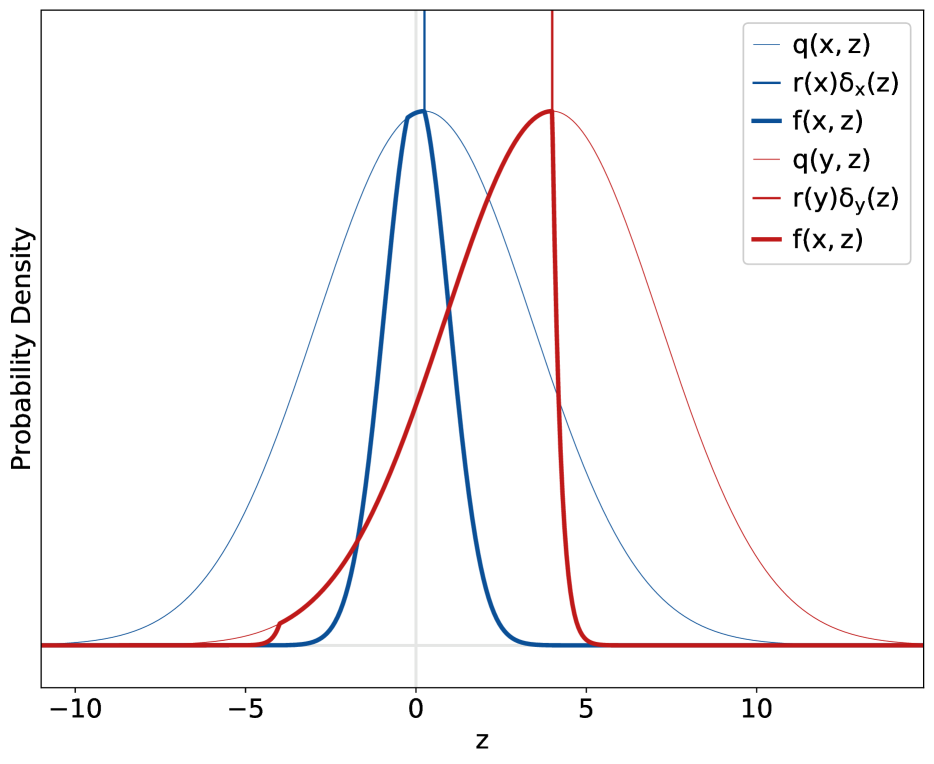
Figure 1: Proposal densities $q$ and MH transition densities $f$, with ${\pi=\operatorname{N}(0,1)}$, $x=1/4$, $y=4$, and $Q(z,\cdot)=\operatorname{N}(z,10)$. $P(x,\cdot)$ and $P(y,\cdot)$ also contain point masses with weights ${r(x)\approx 0.69}$ and ${r(y)\approx 0.47}$, respectively. The algorithms described in this paper construct couplings of such transition kernels, sometimes by way of proposal distribution couplings.

A probability distribution $\gamma$ on $\mathcal{X}\times\mathcal{X}$ is a coupling of distributions $\mu$ and $\nu$ on $(\mathcal{X},\mathscr{F})$ if ${\gamma(A\times\mathcal{X})=\mu(A)}$ and ${\gamma(\mathcal{X}\times A)=\nu(A)}$ for any ${A\in\mathscr{F}}$. Let $\Gamma(\mu,\nu)$ be the set of all couplings of $\mu$ and $\nu$. We say that a joint kernel $\bar{P}$ is a coupling of $P$ with itself and write $\bar{P}\in\Gamma(P,P)$ if $\bar{P}((x,y,),\cdot)\in\Gamma(P(x,\cdot),P(y,\cdot))$ for any $x,y\in\mathcal{X}$. Similar definitions apply to couplings $\bar{Q}$ of proposal distributions and couplings $\bar{B}$ of acceptance indicators.

The coupling inequality (Levin et al.,, 2017, Proposition 4.7) states that the meeting probability ${\operatorname{\mathbb{P}}_{(X,Y)\sim\gamma}(X=Y)\leq 1-\lVert\mu-\nu\rVert_{\sf TV}}$ for any coupling $\gamma\in\Gamma(\mu,\nu)$. Here ${\lVert\mu-\nu\rVert_{\sf TV}=\sup_{A\in\mathscr{F}}|\mu(A)-\nu(A)|}$ is the total variation distance. A coupling that achieves this bound is said to be maximal, and we write $\Gamma^{\mathrm{max}}(\mu,\nu)\subset\Gamma(\mu,\nu)$ for the set of maximal couplings of $\mu$ and $\nu$.

2.2 Status Quo: the Heuristic Coupling $\bar{P}_{\mathrm{SQ}}$

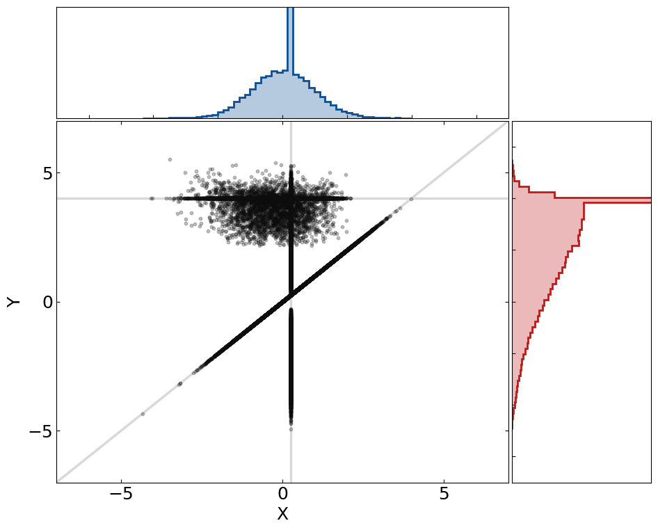
Figure 2: Draws from the coupling $\bar{P}_{\mathrm{SQ}}((x,y),\cdot)$ using $\bar{Q}_{\mathrm{MI}}$ and the same parameters as in Figure 1. The grey lines indicate $X=x$, $Y=y$, and $X=Y$, while the histograms show the marginal distributions of $X$ and $Y$.

We begin by describing the state-of-the-art coupling of MH transition kernels, first introduced in Johnson, (1998). Recall that draws from a MH-like kernel $P(x,\cdot)$ can be obtained via a proposal ${x^{\prime}\sim Q(x,\cdot)}$ which is accepted for $X$ with probability $a(x,x^{\prime})$. Thus a simple way to couple $P$ with itself is to draw coupled proposals ${(x^{\prime},y^{\prime})\sim\bar{Q}((x,y),\cdot)}$ and accept or reject these according to coupled indicators ${(B_{x},B_{y})\sim\bar{B}((x,y),(x^{\prime},y^{\prime}))}$, where ${\bar{Q}\in\Gamma(Q,Q)}$ and $\bar{B}((x,y),(x^{\prime},y^{\prime}))\in\Gamma\big{(}\!\operatorname{Bern}(a(x,x^{\prime})),\operatorname{Bern}(a(y,y^{\prime}))\big{)}$. We refer to this coupling as $\bar{P}_{\mathrm{SQ}}$ and summarize it in Algorithm 1.

Algorithm 1 Draw $(X,Y)\sim\bar{P}_{\mathrm{SQ}}((x,y),\cdot)$

1. Draw $(x^{\prime},y^{\prime})\sim\bar{Q}((x,y),\cdot)$

2. Draw $(B_{x},B_{y})\sim\bar{B}((x,y),(x^{\prime},y^{\prime}))$

3. Set $X\>\!=\>\!B_{x}\,x^{\prime}+(1-B_{x})x$ and $Y\>\!=\>\!B_{y}\,y^{\prime}+(1-B_{y})y$

4. Return $(X,Y)$

For the chains to meet in finite time we need ${\operatorname{\mathbb{P}}(X=Y\mid x,y)>0}$ from at least some states $(x,y)$, which in turn requires ${\operatorname{\mathbb{P}}(x^{\prime}=y^{\prime}\mid x,y)>0}$. To obtain this we take the joint proposal distribution $\bar{Q}$ to be a maximal coupling of $Q$ with itself. We can draw from such a coupling by sampling $x^{\prime}\sim Q(x,\cdot)$, using this as a rejection sampling proposal for $Q(y,\cdot)$, and drawing $y^{\prime}$ in a specified way if this $x^{\prime}=y^{\prime}$ proposal is rejected. This approach achieves the coupling inequality upper bound ${\operatorname{\mathbb{P}}(x^{\prime}=y^{\prime}\mid x,y)=1-\int q(x,z)\wedge q(y,z)\,\mathrm{d}z}$.

Algorithm 2 Draw $(x^{\prime},y^{\prime})\sim\bar{Q}_{\mathrm{MI}}((x,y),\cdot)$

1. Draw $x^{\prime}\sim Q(x,\cdot)$ and $U\sim\operatorname{Unif}$

2. If $Uq(x,x^{\prime})\leq q(y,x^{\prime})$, set $y^{\prime}=x^{\prime}$

3. Else

   1. Draw $\tilde{y}\sim Q(y,\cdot)$ and $V\sim\operatorname{Unif}$

   2. If $Vq(y,\tilde{y})>q(x,\tilde{y})$, set $y^{\prime}=\tilde{y}$

   3. Else go to 3(a)

4. Return $(x^{\prime},y^{\prime})$

A simple example of this method is the maximal coupling with independent residuals $\bar{Q}_{\mathrm{MI}}$, introduced in Vaserstein, (1969) and called the $\gamma$-coupling in Lindvall, (1992, chap. 1.5). It has the property that $x^{\prime}$ and $y^{\prime}$ are independent when $x^{\prime}\neq y^{\prime}$. Algorithm 2 describes how to draw from this coupling, and Figure 2 illustrates a set of draws $(X,Y)\sim\bar{P}_{\mathrm{SQ}}((x,y),\cdot)$ based on proposals from $\bar{Q}_{\mathrm{MI}}$.

When $\mathcal{X}=\mathbb{R}^{d}$ and $Q$ is spherically symmetric, the maximal coupling with reflection residuals, $\bar{Q}_{\mathrm{MR}}$, is often a better alternative. This coupling was introduced in the context of Hamiltonian and Langevin methods (Bou-Rabee et al.,, 2020; Eberle et al.,, 2019) and has its origins in the analysis of continuous-time processes (Lindvall and Rogers,, 1986; Eberle,, 2011). $\bar{Q}_{\mathrm{MR}}$ is identical to $\bar{Q}_{\mathrm{MI}}$ for $x^{\prime}=y^{\prime}$. When $x^{\prime}\neq y^{\prime}$ the coupling $\bar{Q}_{\mathrm{MR}}$ sets $y^{\prime}=T_{xy}(x^{\prime})$, where $T_{xy}(x^{\prime})=y+(I-2ee^{\prime})(x^{\prime}-x)$ and $e=(y-x)/\lVert y-x\rVert$. We define $T_{yx}(y^{\prime})$ similarly. Note that the transformation $z\to(I-2ee^{\prime})z$ reflects the $e$ component of $z$ while leaving the $e^{\perp}$ component fixed.

A standard choice for the acceptance indicators $(B_{x},B_{y})\sim\bar{B}((x,y),(x^{\prime},y^{\prime}))$ is the unique maximal coupling of $\operatorname{Bern}(a(x,x^{\prime}))$ and $\operatorname{Bern}(a(y,y^{\prime}))$, which can be realized by drawing $U\sim\operatorname{Unif}$ and setting ${B_{x}=1(U\leq a(x,x^{\prime}))}$ and ${B_{y}=1(U\leq a(y,y^{\prime}))}$. Among couplings of these distributions, this one yields the maximal probability ${\operatorname{\mathbb{P}}(B_{x}=B_{y}=1\mid x^{\prime},y^{\prime})}={a(x,x^{\prime})\wedge a(y,y^{\prime})}$. Other objectives, such as the minimization of $\operatorname{\mathbb{E}}[\lVert X-Y\rVert\mid x^{\prime},y^{\prime}]$, are also possible.

The coupling $\bar{P}_{\mathrm{SQ}}$ obtained when $\bar{Q}$ is a maximal coupling of proposal distributions and $\bar{B}$ is the maximal coupling of acceptance indicators can yield a relatively high chance of ${X=Y}$ given the current state pair $(x,y)$, but it typically falls short of the theoretical upper bound. Under $\bar{P}_{\mathrm{SQ}}$, the probability of $X=Y$ is ${\int\!\big{(}q(x,z)\wedge q(y,z)\big{)}\big{(}a(x,z)\wedge a(y,z)\big{)}\,\mathrm{d}z}$. However Lemma 1 implies that the coupling inequality bound is $\int\!\big{(}q(x,z)a(x,z)\big{)}\wedge\big{(}q(y,z)a(y,z)\big{)}\,\mathrm{d}z$, which is always an equal or larger quantity. Figure 3 illustrates the gap between the meeting probabilities under $\bar{P}_{\mathrm{SQ}}$ and under any maximal coupling $\bar{P}$. Note that these probabilities will coincide when either $q(x,z)$ or $a(x,z)$ does not depend on $x$, e.g. for the independence sampler.

Lemma 1.

Let $P$ be an MH-like transition kernel as defined above. Then for $x\neq y$, ${\lVert P(x,\cdot)-P(y,\cdot)\rVert_{\sf TV}}={1-\int f(x,z)\wedge f(y,z)\,\mathrm{d}z}$.

Proof.

Let $C_{xy}=\{z:f(x,z)>f(y,z)\}\cup\{x\}\setminus\{y\}$ and similarly for $C_{yx}$. We have ${\lVert P(x,\cdot)-P(y,\cdot)\rVert_{\sf TV}}={\sup_{A}|P(x,A)-P(y,A)|}$, and ${|P(x,A)-P(y,A)|}={|\int_{A}f(x,z)\!-\!f(y,z)\,\mathrm{d}z+1(x\in A)r(x)\!-\!1(y\in A)r(y)|.}$ We must have either $A=C_{xy}$ or $A=C_{yx}$ in the supremum above. Both yield the same value, and so $\lVert P(x,\cdot)-P(y,\cdot)\rVert_{\sf TV}=1-\int f(x,z)\wedge f(y,z)\,\mathrm{d}z$. ∎

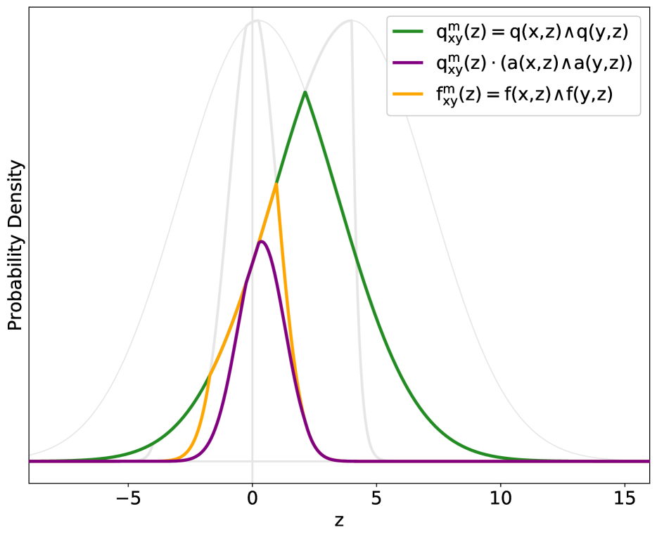
Figure 3: Meeting densities based on the same parameters as in Figure 1. The green line shows the density of ${x^{\prime}=y^{\prime}=z}$ under a maximal coupling $\bar{Q}$. The purple line shows the density of $X=Y=z$ under $\bar{P}_{\mathrm{SQ}}$ assuming the use of a maximal coupling $\bar{B}$. Finally, the orange line shows the density of $X=Y=z$ under a maximal coupling $\bar{P}$. The inequalities suggested here hold in general.

We want to maximize the coupling probability at each step and reduce typical meeting times, so the factors above lead us to ask if there are couplings $\bar{P}$ which are both implementable and maximal. Our contribution answers this question in the affirmative.

3 Maximal Couplings

We now introduce a collection of implementable couplings ${\bar{P}\in\Gamma^{\mathrm{max}}(P,P)}$ starting from an arbitrary MH-like transition kernel $P$. We consider two approaches. In Sections 3.1 and 3.2 we show how to couple Markov transition kernels without explicitly coupling their underlying proposal or acceptance distributions. We refer to these as full-kernel couplings. In Section 3.3, we modify Algorithm 1 to maximize the probability of accepting proposals $x^{\prime}=y^{\prime}$ at the expense of decreasing the acceptance probabilities when $x^{\prime}\neq y^{\prime}$.

Algorithm 3 Draw $(X,Y)\sim\bar{P}_{\mathrm{MI}}((x,y),\cdot)$

1. Draw $X\sim P(x,\cdot)$ and $U\sim\operatorname{Unif}$

2. If $X\neq x$ and $U\,f(x,X)\leq f(y,X)$, set $Y=X$

3. Else

   1. Draw $\tilde{y}\sim P(y,\cdot)$ and $V\sim\operatorname{Unif}$

   2. If $\tilde{y}=y$, set $Y=\tilde{y}$

   3. If $\tilde{y}\neq y$ and $V\,f(y,\tilde{y})>f(x,\tilde{y})$, set $Y=\tilde{y}$

   4. Else go to 3(a)

4. Return $(X,Y)$

3.1 $\bar{P}_{\mathrm{MI}}$, a Full-kernel Coupling with Independent Residuals

Our first full-kernel coupling, which we will refer to as $\bar{P}_{\mathrm{MI}}$, is inspired by the procedure described in Algorithm 2 for drawing from the coupling $\bar{Q}_{\mathrm{MI}}$ of proposal distributions. A key difference between coupling proposal distributions and transition kernels is that by assumption the proposal distributions are non-atomic and absolutely continuous with respect to an underlying measure, while MH-like kernels $P$ can have a point mass at the current state. Therefore our rejection sampling procedure must be modified to yield draws $X$ and $Y$ with the correct marginal distributions.

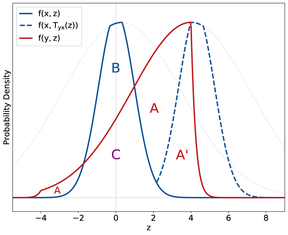
Figure 4: Rejection sampling regions for Algorithms 3 and 4 based on the same parameters as Figure 1. For both options, meeting occurs on samples drawn from region $C$.

Algorithm 3 contains this modification, which we illustrate in Figure 4. The blue and red curves give the continuous parts of $P(x,\cdot)$ and $P(y,\cdot)$, respectively. We think of the algorithm as sampling uniformly from the region under the graph along with point masses at $x$ and $y$. If the $X$ draw falls in $C$ we can use the same point for both chains, and otherwise we use rejection sampling to obtain a $Y$ draw from $A\cup A^{\prime}\cup\{y\}$. Meetings occur exactly on draws from $C$, and thus it occurs with probability $\int f(x,z)\wedge f(y,z)\,\mathrm{d}z$. See Appendix A.1 for a detailed proof that $\bar{P}_{\mathrm{MI}}((x,y),\cdot)$ is a maximal coupling of $P(x,\cdot)$ and $P(y,\cdot)$ and an analysis of the computation cost of this algorithm.

3.2 $\bar{P}_{\mathrm{MR}}$, a Full-kernel Coupling with Reflection Residuals

All maximal couplings of a given $P$ have equal meeting probability, but some perform better than others. Although $\operatorname{\mathbb{P}}(X=Y\mid x,y)$ is maximal under $\bar{P}_{\mathrm{MI}}((x,y),\cdot)$, $X$ and $Y$ are independent when ${X\neq Y}$. This creates a strong tendency for $\lVert Y-X\rVert$ to grow with the dimension of the state space, as seen in the experiments of Jacob et al., (2020). Even under a maximal coupling, $\operatorname{\mathbb{P}}(X=Y\mid x,y)$ can be small until $x$ and $y$ are close. Thus the time for a pair of coupled chains to meet depends on both the meeting probability from each state pair and the degree of contraction between chains when meeting does not occur.

The advantages of using $\bar{Q}_{\mathrm{MR}}$ vs. $\bar{Q}_{\mathrm{MI}}$ in Algorithm 1 appear to be due to this consideration. See Section 4.2 below for numerical justifications. It also motivates the following full-kernel maximal coupling with reflection residuals, which we refer to as $\bar{P}_{\mathrm{MR}}$ and describe in detail in Algorithm 4. For this algorithm define ${f^{m}_{xy}(z):=f(x,z)\wedge f(y,z)}$, ${\tilde{f}^{r}_{xy}(x^{\prime}):=f(x,x^{\prime})-f_{xy}^{m}(x^{\prime})}$, and likewise for $\tilde{f}^{r}_{yx}(y^{\prime})$. Finally set ${\tilde{f}^{t}_{yx}(y^{\prime}):=\tilde{f}^{r}_{yx}(y^{\prime})-\tilde{f}^{r}_{yx}(y^{\prime})\wedge\tilde{f}^{r}_{xy}(T_{yx}(y^{\prime}))}$, the $y$ residual after reflection evaluated at $y^{\prime}$.

Figure 4 provides some intuition into the behavior of $\bar{P}_{\mathrm{MR}}$. The first step of $\bar{P}_{\mathrm{MR}}$ is identical to $\bar{P}_{\mathrm{MI}}$ in that it attempts to draw from the region $C$, and a meeting occurs if this is successful. Otherwise $\bar{P}_{\mathrm{MR}}$ proposes the reflected point $T_{xy}(X)$ for $Y$, which succeeds if this point falls in the region $A^{\prime}$. If all else fails, we use rejection sampling to obtain a $Y$ draw from $A\cup\{y\}$. See Appendix A.2 for a detailed proof of the validity and maximality, and an analysis of the computation cost of $\bar{P}_{\mathrm{MR}}$.

Algorithm 4 Draw $(X,Y)\sim\bar{P}_{\mathrm{MR}}((x,y),\cdot)$

1. Draw $X\sim P(x,\cdot)$ and $U\sim\operatorname{Unif}$

2. If $X\neq x$ and $Uf(x,X)\leq f(y,X)$, set $Y=X$

3. Else

   1. Set $\tilde{y}=T_{xy}(X)$ and draw $V\sim\operatorname{Unif}$

   2. If $X\>\!\neq\>\!x$ and $Vf^{r}_{xy}(X)\>\!\leq\>\!\tilde{f}^{r}_{yx}(\tilde{y})$, set $Y\>\!=\>\!\tilde{y}$

   3. Else

      1. Draw $\tilde{y}\sim P(y,\cdot)$ and $W\sim\operatorname{Unif}$

      2. If $\tilde{y}=y$, set $Y=\tilde{y}$

      3. If $\tilde{y}\>\!\neq\>\!y$ and $Wf(y,y^{\prime})\>\!\leq\>\!\tilde{f}^{t}_{yx}(\tilde{y})$, set $Y\>\!=\>\!\tilde{y}$

      4. Else go to 3(c)i.

4. Return $(X,Y)$

3.3 Maximal Coupled Transitions from Maximally Coupled Proposals with $\bar{P}_{\mathrm{C}}$

While the coupling $\bar{P}_{\mathrm{MR}}$ sometimes outperforms $\bar{P}_{\mathrm{MI}}$, it also has a few limitations. First, the reflection proposal strategy requires a high degree of reflection symmetry between the distributions of $X$ and $Y$ conditional on $X\neq Y$ to be successful. For example in the setting of Figure 4, the reflection proposal has more than a 50% chance of being rejected. Without such a symmetry $X$ and $Y$ will tend to be conditionally independent, resulting in poor contraction between chains when meeting does not occur.

Second, any full-kernel coupling is constrained to work directly with the complicated and irregular geometry of $P$ rather than the simple and often tractable form of the proposal distribution $Q$. In contrast to the range of couplings and optimal transport strategies available when a standard distribution is used for $Q$, it appears to be more difficult to design high-performance couplings directly in terms of the associated transition kernels $P$.

Algorithm 5 Draw $(X,Y)\sim\bar{P}_{\mathrm{C}}((x,y),\cdot)$

1. Draw $(x^{\prime},y^{\prime})\sim\bar{Q}((x,y),\cdot)$

2. If $x^{\prime}=y^{\prime}$ set $\bar{B}=\bar{B}_{1}$, else set $\bar{B}=\bar{B}_{2}$

3. Draw $(B_{x},B_{y})\sim\bar{B}((x,y),(x^{\prime},y^{\prime}))$

4. Set $X\>\!=\>\!B_{x}\,x^{\prime}+(1-B_{x})x$ and $Y\>\!=\>\!B_{y}\,y^{\prime}+(1-B_{y})y$

5. Return $(X,Y)$

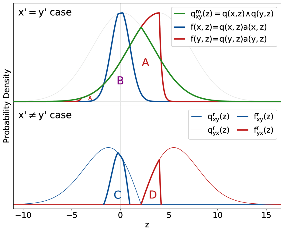
Figure 5: Distributions used in Algorithm 5 based on the same parameters as Figure 1. Upper pane: draws ${x^{\prime}=y^{\prime}}$ follow $q^{m}$ and are used as proposals for $f(x,\cdot)$ and $f(y,\cdot)$. Lower pane: Draws $x^{\prime}\neq y^{\prime}$ follow the proposal residuals $q^{r}$ and are used as rejection sampling proposals for the transition kernel residuals $f^{r}$.

This motivates the next coupling, which allows the use of any coupling of $Q$ while still possibly achieving the maximal coupling probability identified in Lemma 1. We refer to this new algorithm as $\bar{P}_{\mathrm{C}}$, since it resembles $\bar{P}_{\mathrm{SQ}}$ up to the conditional use of one or another Bernoulli coupling $\bar{B}$ depending on whether or not a meeting is proposed. Together with the definitions below, Algorithm 5 shows how to draw from $\bar{P}_{\mathrm{C}}$. We can choose a maximal $\bar{Q}$ such as $\bar{Q}_{\mathrm{MI}}$ or $\bar{Q}_{\mathrm{MR}}$ to obtain a maximal $\bar{P}$, although we also obtain a valid $\bar{P}\in\Gamma(P,P)$ for non-maximal choices of $\bar{Q}$.

To define $\bar{P}_{\mathrm{C}}$, let $q^{m}_{xy}(\cdot)$ be the density of $\bar{Q}((x,y),\cdot)$ on $\Delta=\{(z,z):z\in\cal X\}$. We establish the existence and properties of $q^{m}_{xy}$ in Lemma 2, below. Define the proposal residual ${q^{r}_{xy}(x^{\prime}):={q(x,x^{\prime})-q_{xy}^{m}(x^{\prime})}}$ and the transition kernel residual ${f_{xy}^{r}(x^{\prime}):=0\vee(f(x,x^{\prime})-q_{xy}^{m}(x^{\prime}))}$, and similarly for $q^{r}_{yx}(y^{\prime})$ and $f^{r}_{yx}(y^{\prime})$. We illustrate these functions in Figure 5.

Lemma 2.

If $\bar{Q}\in\Gamma(Q,Q)$ then there exists a density $q^{m}_{xy}$ for $\bar{Q}((x,y),\cdot)$ on $\Delta$. If $\bar{Q}$ is a maximal coupling, then $q^{m}_{xy}(z)=q(x,z)\wedge q(y,z)$ for almost all $z$.

Proof.

Let $\lambda$ denote the base measure on $(\mathcal{X},\mathscr{F})$ and let $\lambda_{\Delta}$ be its push-forward to $\Delta$ by the map ${z\mapsto(z,z)}$. Since $\mathcal{X}$ is a Polish space, we have ${A_{\Delta}:=\{(z,z):z\in A\}\in\mathscr{F}\otimes\mathscr{F}}$ for any ${A\in\mathscr{F}}$. Thus $\bar{Q}((x,y),\cdot)$ induces a sub-probability $\bar{Q}_{\Delta}$ on $\Delta$. Also ${\bar{Q}_{\Delta}\ll\lambda_{\Delta}}$, since if ${\lambda_{\Delta}(A_{\Delta})=\lambda(A)=0}$ then ${\bar{Q}_{\Delta}(A_{\Delta})\leq\bar{Q}((x,y),A\times\mathcal{X})=Q(x,A)=0}$. The Radon–-Nikodym theorem then guarantees the existence of an integrable function ${q^{m}_{xy}:\mathcal{X}\to[0,\infty)}$ such that ${\bar{Q}((x,y),A_{\Delta})=\int_{A}q^{m}_{xy}(z)\,\mathrm{d}z}$.

Next, we claim ${q^{m}_{xy}(z)\leq q(x,z)\wedge q(y,z)}$ for $\lambda$-almost all $z$. Let ${A:=\{z:q^{m}_{xy}(z)>q(x,z)\wedge q(y,z)\}\in\mathscr{F}}$, ${A_{x}:=\{z:q^{m}_{xy}(z)>q(x,z)\}\in\mathscr{F}}$, and likewise for $A_{y}$. Since $A=A_{x}\cup A_{y}$, $\lambda(A)>0$ implies $\lambda(A_{x})>0$ or $\lambda(A_{y})>0$. If $\lambda(A_{x})>0$ then ${\bar{Q}((x,y),A_{x}\times\mathcal{X})}={Q(x,A_{x})}<{\bar{Q}((x,y),(A_{x})_{\Delta})}\leq{\bar{Q}((x,y),A_{x}\times\mathcal{X})}$, a contradiction. The case $\lambda(A_{y})>0$ similarly implies a contradiction, so we conclude that $\lambda(A)=0$.

Finally, if $\bar{Q}$ is maximal, a total variation computation similar to that of Lemma 1 shows that $\bar{Q}((x,y),\Delta)=\int q(x,z)\wedge q(y,z)\,\mathrm{d}z$. Combining this with the above implies $q^{m}_{xy}(z)=q(x,z)\wedge q(y,z)$ for $\lambda$-almost all $z$. ∎

Resuming our definition of $\bar{P}_{\mathrm{C}}$, we set acceptance probabilities $b_{xy}(x^{\prime}):={1\wedge(f(x,x^{\prime})/q_{xy}^{m}(x^{\prime}))}$ if ${q_{xy}^{m}(x^{\prime})>0}$ or else ${b_{xy}(x^{\prime}):=1}$, ${c_{xy}(x^{\prime}):=f^{r}_{xy}(x^{\prime})/q^{r}_{xy}(x^{\prime})}$ if $q^{r}_{xy}(x^{\prime})=0$ or else $c_{xy}(x^{\prime}):=1$, and likewise for $b_{yx}(y^{\prime})$ and $c_{yx}(y^{\prime})$. When $x^{\prime}=y^{\prime}$ we require that the acceptance indicator pair $(B_{x},B_{y})$ follows the maximal coupling $\bar{B}_{1}$ of $\operatorname{Bern}(b_{xy}(x^{\prime}))$ and $\operatorname{Bern}(b_{yx}(y^{\prime}))$. When ${x^{\prime}\neq y^{\prime}}$ we require that $(B_{x},B_{y})$ follows any coupling ${\bar{B}_{2}\in\Gamma(\operatorname{Bern}(c_{xy}(x^{\prime})),\operatorname{Bern}(c_{yx}(y^{\prime})))}$. Simulation results suggest that maximal couplings for $\bar{B}_{2}$ perform well, but optimal transport couplings which aim to minimize $\lVert X-Y\rVert$ are also attractive in this setting.

When $\bar{Q}$ proposes a meeting $x^{\prime}=y^{\prime}$, we think of $\bar{P}_{\mathrm{C}}$ as using these values as rejection sampling proposals for the transition distributions $f(x,z)$ and $f(y,z)$. This results in a higher marginal acceptance rate than we would have under MH. On the other hand when $x^{\prime}\neq y^{\prime}$. we think of this method as falling back to rejection sampling of the residual distributions $f$ from the residuals distributions of $q$, both after the removal of $q_{xy}^{m}$. This produces a lower marginal acceptance rate than MH, exactly counterbalancing the above. In Proposition 1 we show that $\bar{P}_{\mathrm{C}}((x,y),\cdot)$ is a maximal coupling of $P(x,\cdot)$ and $P(y,\cdot)$.

Proposition 1.

For any $\bar{Q}\in\Gamma(Q,Q)$, the output $(X,Y)$ of Algorithm 5 will follow a coupling ${\bar{P}\in\Gamma(P,P)}$. If $\bar{Q}$ is maximal then $\bar{P}$ will be as well.

Proof.

At any point $x^{\prime}\neq x$, $X$ will have density

$$q^{m}_{xy}(x^{\prime})b_{xy}(x^{\prime})+q^{r}_{xy}(x^{\prime})c_{xy}(x^{\prime})$$

$$=\big{(}q^{m}_{xy}(x^{\prime})\wedge f(x,x^{\prime})\big{)}+\big{(}q^{r}_{xy}(x^{\prime})\wedge f^{r}_{xy}(x^{\prime})\big{)}$$

$$=\big{(}q^{m}_{xy}(x^{\prime})\wedge f(x,x^{\prime})\big{)}+f^{r}_{xy}(x^{\prime})=f(x,x^{\prime}).$$

The second equality holds because ${f^{r}_{xy}(x^{\prime})\leq q^{r}_{xy}(x^{\prime})}$. This in turn holds because $f(x,x^{\prime})\leq q(x,x^{\prime})$ and ${q^{m}_{xy}(x^{\prime})\leq q(x,x^{\prime})}$ by Lemma 2, so

$$f^{r}_{xy}(x^{\prime}) ={\big{(}f(x,x^{\prime})\vee q^{m}_{xy}(x^{\prime})\big{)}-q^{m}_{xy}(x^{\prime})}$$

$$\leq q(x,x^{\prime})-q^{m}_{xy}(x^{\prime})=q^{r}_{xy}(x^{\prime}).$$

Integrating the density of $X$ over all $x^{\prime}\neq x$ yields $\operatorname{\mathbb{P}}(X=x)={1-\int f(x,x^{\prime})\,\mathrm{d}x^{\prime}}=r(x)$, so we conclude $X\sim P(x,\cdot)$. A similar argument shows that ${Y\sim P(y,\cdot)}$. Thus $(X,Y)$ follows the desired coupling.

If $\bar{Q}$ is maximal then by Lemma 2 the probability density at the proposal $(z,z)\sim\bar{Q}((x,y),\cdot)$ will be $q^{m}_{xy}(z)=q(x,z)\wedge q(y,z)$. By the definition of $\bar{B}_{1}$, the probability of accepting a proposal $x^{\prime}=y^{\prime}=z$ for both $X$ and $Y$ will be

$$\big{(}1\wedge\tfrac{f(x,z)}{q^{m}_{xy}(z)}\big{)}\wedge\big{(}1\wedge\tfrac{f(y,z)}{q^{m}_{yx}(z)}\big{)}=\tfrac{f(x,z)\wedge f(y,z)}{q(x,z)\wedge q(y,z)}.$$

Combining this with the proposal density implies that the overall coupled transition kernel density at ${X=Y=z}$ will be $f(x,z)\wedge f(y,z)$. Thus $\operatorname{\mathbb{P}}(X=Y)={\int f(x,z)\wedge f(y,z)\,\mathrm{d}z}$, and by Lemma 1 we conclude that $\bar{P}$ is maximal. ∎

We observe that $\bar{P}_{\mathrm{C}}$ matches the flexibility and computational efficiency of $\bar{P}_{\mathrm{SQ}}$ while offering a higher meeting probability at each iteration. The ability to chose an arbitrary $\bar{Q}\in\Gamma(Q,Q)$ is also a significant advantage of $\bar{P}_{\mathrm{C}}$ over the full-kernel couplings. The extra effort required to construct, validate, and draw from $\bar{P}_{\mathrm{MR}}$ relative to $\bar{P}_{\mathrm{MI}}$ shows how challenging such refinements can be. Finally, we note that $\bar{P}_{\mathrm{C}}$ can be more computationally efficient than the full-kernel couplings $\bar{P}_{\mathrm{MI}}$ and $\bar{P}_{\mathrm{MR}}$, in that it avoids the ‘while’ loops of Step 3 of Algorithms 3 and 4.

4 Numerical Examples

4.1 Biased Random Walk MH

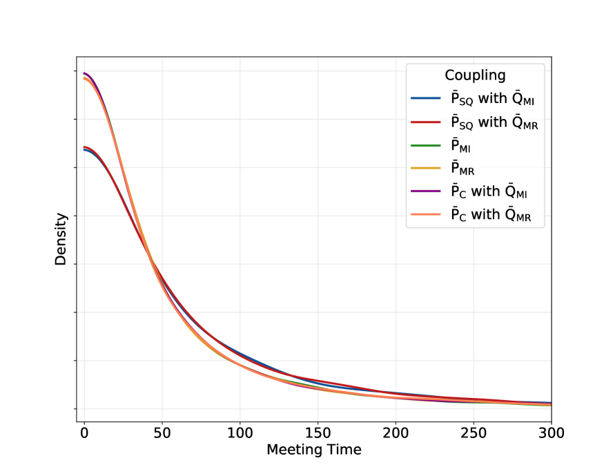
Figure 6: Distribution of meeting times for the example described in Section 4.1. The four maximal couplings yield almost identical distributions of shorter meeting times times while the two $\bar{P}_{\mathrm{SQ}}$ methods yield almost identical distribution of longer ones. In this example the requirement that $\bar{P}_{\mathrm{SQ}}$ accept meeting and non-meeting proposals at exactly the MH rate puts it at a significant disadvantage vs. the maximal couplings.

For our first example we consider a toy model that emphasizes the differences between $\bar{P}_{\mathrm{SQ}}$ and the maximal couplings $\bar{P}_{\mathrm{MI}}$, $\bar{P}_{\mathrm{MR}}$, and $\bar{P}_{\mathrm{C}}$. We assume an Exponential target distribution $\pi=\operatorname{Expo}(1)$ and draw proposals from ${Q(z,\cdot)=\operatorname{N}(z+\kappa,\sigma^{2})}$ with $\kappa>0$. We then accept or reject these proposals at the usual MH rate, so ${a(z,z^{\prime})=1\wedge\exp\!\big{(}(z-z^{\prime})(2\kappa/\sigma^{2}+1)\big{)}}$. Our assumption on $\kappa$ implies $a(x,z)\wedge a(y,z)=a(x,z)$ if $x\leq y$ and $a(x,z)=1$ if $z\leq x$. Thus $Q$ will tend to propose increasing values while $a$ favors decreasing ones. This tension between the proposal and target distributions is characteristic of MH kernels that do not mix rapidly.

We construct the transition kernel couplings $\bar{P}_{\mathrm{SQ}}$ with $\bar{Q}_{\mathrm{MI}}$, $\bar{P}_{\mathrm{MI}}$, $\bar{P}_{\mathrm{MR}}$, and $\bar{P}_{\mathrm{C}}$ with $\bar{Q}_{\mathrm{MI}}$ as described in Sections 2 and 3. We also define a simple generalization of the maximal coupling with reflection residuals, such that either $x^{\prime}=y^{\prime}$ or ${y^{\prime}-(y+\kappa)}={(x+\kappa)-x^{\prime}}$. We use the resulting $\bar{Q}_{\mathrm{MR}}$ as an alternative proposal kernel coupling for $\bar{P}_{\mathrm{SQ}}$ and $\bar{P}_{\mathrm{C}}$. We set $\kappa=\sigma^{2}=3$, draw initial values independently from the target $\pi$, and run 10,000 replications for each coupling option. For each replication we record the meeting time ${\tau=\min(t\geq 0:X_{t}=Y_{t})}$. As described in Section 1, such meeting times are of theoretical and practical importance, and they also make a good measure of coupling performance. We summarize the average behavior of these meeting times in Table 1 and present their full distribution in Figure 6.

Table 1: Section 4.1 Example Results

Coupling	Avg. Meeting Time	S.E.
$\bar{P}_{SQ}$ with $\bar{Q}_{MI}$	74.0	0.94
$\bar{P}_{SQ}$ with $\bar{Q}_{MR}$	75.6	0.99
$\bar{P}_{MI}$	60.5	0.84
$\bar{P}_{MR}$	60.9	0.87
$\bar{P}_{C}$ with $\bar{Q}_{MI}$	61.3	0.87
$\bar{P}_{C}$ with $\bar{Q}_{MR}$	62.2	0.89

We find that both non-maximal couplings deliver average meeting times around 75 iterations, while the four maximal couplings deliver meeting times around 61 iterations. We recall that for a given state pair $(x,y)$, the maximal couplings produce one value of $\operatorname{\mathbb{P}}(X=Y\mid x,y)$ and two $\bar{P}_{\mathrm{SQ}}$ couplings produce another. The observed clustering of algorithms is consistent with the idea that in this example meeting times are driven by these one-step meeting probabilities rather than by behavior when meeting does not occur, which varies significantly by algorithm.

For a better understanding of these differences, we contrast the behavior of $\bar{P}_{\mathrm{SQ}}$ and $\bar{P}_{\mathrm{C}}$. Although we use the same underlying proposal coupling ${(x^{\prime},y^{\prime})\sim\bar{Q}((x,y),\cdot)}$ in each case, the two MH transition kernel coupligns differ in that $\bar{P}_{\mathrm{SQ}}$ accept its proposals at exactly the MH rate while $\bar{P}_{\mathrm{C}}$ uses a higher acceptance probability when $x^{\prime}=y^{\prime}$ and a lower one when $x^{\prime}\neq y^{\prime}$. In this example, most proposals have a relatively low MH acceptance probability to begin with. Thus $\bar{P}_{\mathrm{C}}$ meets more quickly by concentrating the little acceptance probability available on the draws where they could result in a meeting $X=Y$, while $\bar{P}_{\mathrm{SQ}}$ is forced to accept its proposals at the same relatively low rate whether or not a meeting is proposed.

The above leads us to expect that maximal couplings might provide the greatest advantage over the status quo when low acceptance probabilities are typical, either due to the presence of a challenging target, an imperfect proposal distribution, or both. This example emphasizes simplicity over realism, but we would expect its principles to hold more broadly, especially in cases where mixing is relatively slow.

4.2 Dimension Scaling with a Normal Target

For our second example we consider MH on $\mathbb{R}^{d}$ with a target distribution ${\pi=\operatorname{N}(0,I_{d})}$ and proposals $Q(z,\cdot)=\operatorname{N}(z,I_{d}\,\sigma^{2}_{d})$. Following e.g. Roberts et al., (1997) and Christensen et al., (2005) we set $\sigma^{2}_{d}=\ell^{2}/d$ with $\ell=2.38$. This example allows us to consider the role of the dimension and examine differences between the couplings when meeting probabilities are just one important aspect of their behavior.

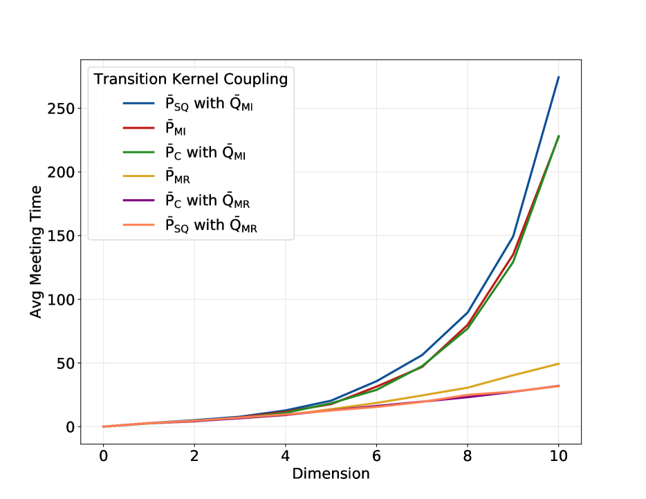
Figure 7: Average meeting times for a range of transition kernel couplings, as described in Section 4.2. Coupling strategies that involve reflections of the proposals appear to outperform the others; among the others, maximal couplings seem to perform better than non-maximal ones.

As above, our main object of interest in this example is the number of iterations required for a pair of coupled chains to meet. We initialize chains on independent draws from $\pi$, consider dimensions $d=1,\dots,10$, and run 1,000 replications for each algorithm. We use a maximal coupling of acceptance indicators for $\bar{P}_{\mathrm{SQ}}$ and $\bar{P}_{\mathrm{C}}$, which appears to yield the best results among the simple acceptance indicator couplings.

We present the results of this experiment in Figure 7. There we observe that $\bar{P}_{\mathrm{SQ}}$ using $\bar{Q}_{\mathrm{MI}}$, $\bar{P}_{\mathrm{C}}$ using $\bar{Q}_{\mathrm{MI}}$, and $\bar{P}_{\mathrm{MI}}$ seem to yield meeting times that increase exponentially in dimension, although the maximal couplings outperform the non-maximal coupling. This blow-up is expected since these options involve independent or weakly dependent behavior when $X\neq Y$. The coupling $\bar{P}_{\mathrm{MR}}$ delivers somewhat better behavior, with $\bar{P}_{\mathrm{SQ}}$ and $\bar{P}_{\mathrm{C}}$ with $\bar{Q}_{\mathrm{MR}}$ delivering the best performance. In higher dimensions it appears that the $\bar{Q}_{\mathrm{MR}}$ version of $\bar{P}_{\mathrm{SQ}}$ may outperform its $\bar{P}_{\mathrm{C}}$ counterpart, an interesting and perhaps counterintuitive result.

To understand these differences in meeting times, we must consider what happens under each coupling $\bar{P}$ when a meeting does not occur. For ${Q(z,\cdot)=\operatorname{N}(z,I_{d}\sigma^{2}_{d})}$, any $\bar{Q}\in\Gamma^{\mathrm{max}}(Q,Q)$ will yield ${\operatorname{\mathbb{P}}(x^{\prime}=y^{\prime}|x,y)=\operatorname{\mathbb{P}}(\chi^{2}_{1}\geq\lVert y-x\rVert^{2}/(4\sigma^{2}_{d}))}$, see e.g. Pollard, (2005, chap. 3.3). Since a meeting cannot occur unless one is proposed, this expression is an upper bound on $\operatorname{\mathbb{P}}(X=Y\mid x,y)$. Thus we should expect the probability of $X=Y$ to fall off rapidly in $\lVert y-x\rVert$, so that couplings which do not promote contraction between chains in the absence of meeting will yield rapidly increasing meeting times.

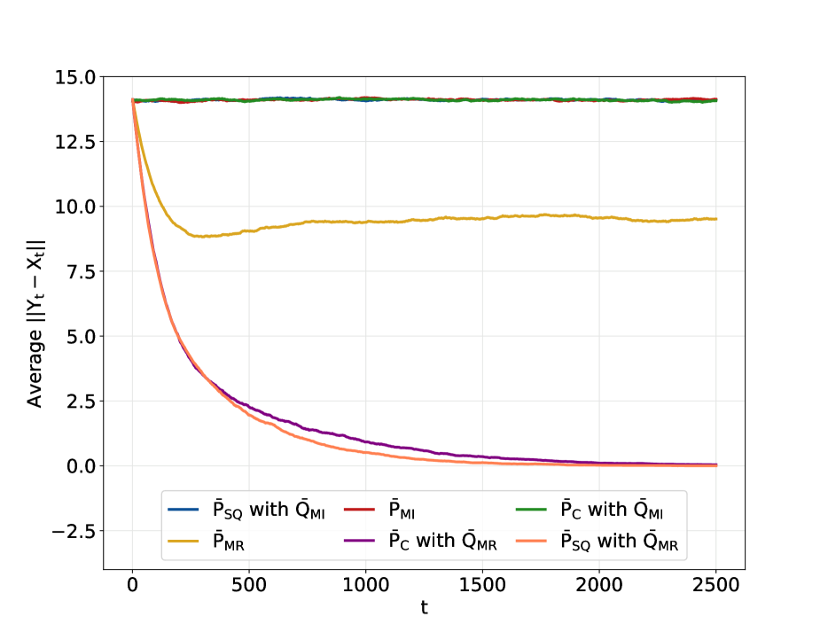
Figure 8: Distance between coupled MH chains by iteration, as described in Section 4.2. Couplings in which $X\neq Y$ implies $X,Y$ independent or almost independent display little contraction, while those based on the maximal reflection coupling of proposal distributions $\bar{Q}_{\mathrm{MR}}$ display strong contraction.

Figure 8 is consistent with these observations. As above we run 1,000 replications per algorithm, initializing each chain with an independent draw from the target distribution. We set $d=100$ to isolate the effects of contraction due to meeting from other contractive behavior and then track the average distance between chains as a function of iteration.

We find that $\bar{P}_{\mathrm{MI}}$, $\bar{P}_{\mathrm{SQ}}$ with $\bar{Q}_{\mathrm{MI}}$, and $\bar{P}_{\mathrm{C}}$ with $\bar{Q}_{\mathrm{MI}}$ produce little or no contraction within the distance achieved by independent draws from the target. They then remain far enough apart that the probability of meeting is negligible. The coupling $\bar{P}_{\mathrm{MR}}$ displays contraction up to a point. Finally we observe that both the maximal and non-maximal couplings based on $\bar{Q}_{\mathrm{MR}}$ contract rapidly to within a radius where meeting can occur. $\bar{P}_{\mathrm{SQ}}$ appears to contract more rapidly than $\bar{P}_{\mathrm{C}}$, which is consistent with its slightly stronger performance in high dimensions.

5 Discussion

Couplings play a central role in the analysis of MCMC convergence and increasingly appear in new methods and estimators. Until now, no general-purpose algorithm has been available to sample from a maximal coupling of MH transition kernels. We fill this gap by introducing three such algorithms, which are implementable under the standard assumptions that one can draw proposals from a distribution $Q$ and compute the density $q$ and acceptance rate $a$ at any points of the state space. The proposed couplings are simple to apply and can be used with a variety of MH strategies including the Metropolis-adjusted Langevin algorithm, pseudo-marginal methods, and the MH-within-Gibbs algorithm.

The experiments in Section 4.1 show that the gains from using these methods can be large, especially when there is a tension between the proposal density $q$ and the acceptance rate $a$. On the other hand the example of Section 4.2 shows that maximality is sometimes less important than other properties of a coupling, such as the contraction behavior when a meeting does not occur. The two examples considered here are simple ones, and experiments with a wider range of MH algorithms and target distributions would clarify the strengths and weaknesses of the proposed couplings.

This work raises several questions. First, it it not known if all couplings of MH kernels might be represented in the form of Algorithm 5 for some appropriate choice of proposal and acceptance couplings; see Nüsken and Pavliotis, (2019) for the treatment of a similar question in the setting of continuous-time Markov chains. It would also be interesting to consider the use of sub-maximal proposal distribution couplings in Algorithm 5, as suggested in the comment of Gerber and Lee, (2020) on Jacob et al., (2020).

Both meeting probabilities and contraction rates influence meeting times, and one might wonder about deriving maximally contractive couplings in analogy to the present work on meeting times. Reflection couplings seem particular effective and are known to be optimal in special cases (Lindvall and Rogers,, 1986). In other cases, synchronous or ‘common random number’ couplings yield strong contraction (e.g. Diaconis and Freedman,, 1999). In most other scenarios the user must construct a coupling tailored to the problem at hand. The methods proposed here represent a step forward in coupling design, but many important questions remain.

From a more theoretical point of view, while the MH kernel $P$ is known to be the projection of the proposal $Q$ onto the set of $\pi$-reversible kernels in a certain metric (Billera and Diaconis,, 2001), it is not known how $\bar{Q}$ relates to the set of maximal couplings of $\pi$-reversible kernels. In particular, it would be interesting to know if the strategy proposed in Section 3.3 corresponds to a projection of $\bar{Q}$ onto that set.

Finally the couplings strategies mentioned above are all Markovian. In some cases non-Markovian couplings are known to deliver more satisfactory performance than Markovian ones (e.g. Smith,, 2014). The design of practical non-Markovian couplings for MCMC is a topic deserving further attention.

Acknowledgements

The authors would like to thank Jun Yang, Persi Diaconis, and Niloy Biswas for helpful discussions. Pierre E. Jacob gratefully acknowledges support by the National Science Foundation through grants DMS-1712872 and DMS-1844695.

Appendix A Appendix

In Appendix A.1, we prove that the coupling $\bar{P}_{\mathrm{MI}}((x,y),\cdot)$ described in Algorithm 3 is a maximal coupling of $P(x,\cdot)$ and $P(y,\cdot)$ and analyze its computational cost. Similarly, in Appendix A.2 we prove that the $\bar{P}_{\mathrm{MR}}$ described in Algorithm 4 is valid and maximal and analyze its cost.

A.1 Validity, maximality, and computation cost of $\bar{P}_{\mathrm{MI}}$

We prove that Algorithm 3 defines a coupling of the correct marginal distributions and that it attains the maximum one-step meeting probability.

Proposition 2.

The draws $(X,Y)$ produced by Algorithm 3 follow a maximal coupling of $P(x,\cdot)$ and $P(y,\cdot)$, with the property that $X$ and $Y$ are conditionally independent given $X\neq Y$. Moreover, the coupling probability is maximized among all possible couplings, so that $\bar{P}_{\mathrm{MI}}((x,y),X=Y)=1-\lVert P(x,\cdot)-P(y,\cdot)\rVert_{\sf TV}.$

Proof.

It suffices to show $Y$ has marginal distribution $P(y,\cdot)$ and the coupling probability equals ${1-\lVert P(x,\cdot)-P(y,\cdot)\rVert_{\sf TV}}$. We define the residual measure of $y$ as $\tilde{P}_{yx}(\cdot)\propto r(y)\delta_{y}(\cdot)+\tilde{f}_{yx}^{r}(\cdot)$, where $\delta_{y}$ is the point mass at state $y$ and $\tilde{f}_{yx}^{r}(y^{\prime})\coloneqq f(y,y^{\prime})-f(y,y^{\prime})\wedge f(x,y^{\prime})$ is the ‘unnormalized’ $y$-residual density evaluated at $y^{\prime}$. These definitions are consistent with the ones given in Section 3.2. From this point of view, Step $3$ can be seen as a standard rejection sampler with proposal measure $P(y,\cdot)$ and target measure $\tilde{P}_{yx}(\cdot)$. For any $y^{\prime}\neq y$, let $f_{yx}(y^{\prime})$ denote the transition density of the $Y$-chain from $y$ to $y^{\prime}$. Then $f_{yx}(y^{\prime})$ can be written as

$$f_{yx}(y^{\prime})=f_{yx}(y^{\prime},\text{Step }2)+f_{yx}(y^{\prime},\text{Step }3).$$

The first term works out to $f_{yx}(y^{\prime},\text{Step }2)=f(x,y^{\prime})\wedge f(y,y^{\prime})$, while the second term can be computed as

$$f_{yx}(y^{\prime},\text{Step }3)=\operatorname{\mathbb{P}}(\text{Step 3})f_{yx}(y^{\prime}\mid\text{Step }3)$$

$$=(1-\int f(x,z)\wedge f(y,z)dz)\frac{1}{c(x,y)}\tilde{f}_{yx}^{r}(y^{\prime}).$$

Here $c(x,y)=1-\int f(y,z)\wedge f(x,z)dz$ is the normalizing constant of $\tilde{P}_{yx}(\cdot)$, which also equals $r(y)+\int\tilde{f}^{r}_{yx}(z)dz$.

Putting all the terms together, we have $f_{yx}(y^{\prime})=f(x,y^{\prime})\wedge f(y,y^{\prime})+\tilde{f}^{r}_{yx}(y^{\prime})=f(y,y^{\prime})$ as desired, which justifies the validity of Algorithm 3.

We can also observe that the coupling probability equals the probability that Algorithm 3 stops at Step $2$. Therefore, the coupling probability satisfies

$$\bar{P}_{\mathrm{MI}}((x,y),X=Y)=\int f(x,y^{\prime})\wedge f(y,y^{\prime})dy^{\prime}=1-\lVert P(x,\cdot)-P(y,\cdot)\rVert_{\sf TV}.$$

We conclude that Algorithm 3 maximizes the coupling probability in one step. ∎

We analyze the computation cost of Algorithm 3 as follows. To draw one sample from Algorithm 3, one needs to run Step 1 once with probability $1$, Step 2 once with probability $1-r(x)$, Step 3 for $N$ times where $N$ is a random variable which equals $0$ with probability $1-\lVert P(x,\cdot)-P(y,\cdot)\rVert_{\sf TV}$, and otherwise a Geometric random variable with success probability $\lVert P(x,\cdot)-P(y,\cdot)\rVert_{\sf TV}$. Meanwhile, Step $1$ contains one draw from $P$, Step $2$ contains two evaluations, Step $3$ contains one draw from $P$ and $0$ or $2$ evaluations, with probability $r(y)$ and $1-r(y)$ respectively.

Therefore, the expected number of draws from $P$ is $2$ and the expected number of evaluations is $4-2r(x)-2r(y)$. Taking account of the fact that each draw from $P$ contains one draw from $q$ and one evaluation of the acceptance ratio, then Algorithm 3 contains $2$ draws from $q$ and $6-2r(x)-2r(y)$ evaluations in expectation. The variance of the computing cost depends the total variation distance between $P(x,\cdot)$ and $P(y,\cdot)$, and goes to infinity as $\lVert P(x,\cdot)-P(y,\cdot)\rVert_{\sf TV}$ goes to zero. This can motivate the consideration of sub-maximal coupling strategies, as described in the comment of Gerber and Lee, (2020) on Jacob et al., (2020).

A.2 Validity, maximality, and computation cost of $\bar{P}_{\mathrm{MR}}$

We prove that Algorithm 4 defines a valid coupling and attains the maximal coupling probability.

Proposition 3.

The draws $(X,Y)\sim\bar{P}_{\mathrm{MR}}((x,y),\cdot)$ produced by Algorithm 4 follow a maximal coupling of $P(x,\cdot)$ and $P(y,\cdot)$.

Proof.

As in the proof of Proposition 2, it suffices to show that $Y$ is distributed according to $P(y,\cdot)$ and that the meeting probability equals $1-\lVert P(x,\cdot)-P(y,\cdot)\rVert_{\sf TV}$. Let the functions $f^{m}_{xy}$, $\tilde{f}^{r}_{xy},\tilde{f}^{r}_{yx}$, and $\tilde{f}^{t}_{yx}$ have the definitions given in Section 3.2. For any $y^{\prime}\neq y$, the Markov transition density $f(y,y^{\prime})$ can be written as the sum of three terms:

$$f(y,y^{\prime})=f^{m}_{xy}(y^{\prime})+\tilde{f}^{r}_{yx}(y^{\prime})\wedge\tilde{f}^{r}_{xy}(T_{yx}(y^{\prime}))+\tilde{f}^{t}_{yx}(y^{\prime}).$$ (1)

For any $y^{\prime}\neq y$, let $f_{yx}(y^{\prime})$ denote the transition density of the $Y$-chain from $y$ to $y^{\prime}$ according to Algorithm 4. Then $f_{yx}(y^{\prime})$ can also be written as the sum of three terms:

$$f_{yx}(y^{\prime})=f_{yx}(y^{\prime},\text{Step }2)+f_{yx}(y^{\prime},\text{Step }3(b))+f_{yx}(y^{\prime},\text{Step }3(c)).$$ (2)

We confirm that each term in Formula (2) matches the corresponding term in (1). For the first term, we have

$$f_{yx}(y^{\prime},\text{Step }2) =f(x,y^{\prime})\operatorname{\mathbb{P}}(Uf(x,y^{\prime})\leq f(y,y^{\prime}))=f(y,y^{\prime})\wedge f(x,y^{\prime}).$$

For the second term, let $x^{\prime}=T_{yx}(y^{\prime})$ be the preimage of $y^{\prime}$ through $T_{xy}$. It is not difficult to verify that $T_{xy}^{-1}=T_{yx}$ and that the Jacobian of both $T_{xy}$ and $T_{yx}$ equals $1$. Thus the density of moving from $y$ to $y^{\prime}$ through Step $3(b)$ will be

$$f_{yx}(y^{\prime},\text{Step }3(b)) =\tilde{f}_{xy}^{r}(x^{\prime})\operatorname{\mathbb{P}}(U\tilde{f}_{xy}^{r}(x^{\prime})\leq\tilde{f}_{yx}^{r}(y^{\prime}))\lvert J(T_{xy}^{-1})\rvert=\tilde{f}^{r}_{yx}(y^{\prime})\wedge\tilde{f}^{r}_{xy}(T_{yx}(y^{\prime})).$$

This matches the second term in (1).

Step $3(c)$ is again a rejection sampler with proposal $P(y,\cdot)$ and target ${\tilde{P}^{t}_{yx}(\cdot)\propto r(y)\delta_{y}(\cdot)+\tilde{f}^{t}_{yx}(\cdot)}$. Therefore,

$$f_{yx}(y^{\prime},\text{Step }3(c)) =\operatorname{\mathbb{P}}(\text{Step }3(c))\cdot f_{yx}(y^{\prime}|\text{Step }3(c))=\operatorname{\mathbb{P}}(\text{Step }3(c))\frac{1}{\tilde{c}(x,y)}\tilde{f}_{yx}^{t}(y^{\prime}),$$

where $\tilde{c}(x,y)=1/(r(y)+\int\tilde{f}^{t}_{yx}(z)\,\mathrm{d}z)$ is the normalizing constant of $\tilde{P}^{t}_{yx}(\cdot)$.

Meanwhile, we have

$$\operatorname{\mathbb{P}}(\text{Step }3(c)) =1-\int f^{m}_{xy}(y^{\prime})dy^{\prime}-\int\tilde{f}^{r}_{yx}(y^{\prime})\wedge\tilde{f}^{r}_{xy}(T_{yx}(y^{\prime}))\,\mathrm{d}y^{\prime}$$

$$=r(y)+\int f(y,y^{\prime})\,\mathrm{d}y^{\prime}-\int f^{m}_{xy}(y^{\prime})\,\mathrm{d}y^{\prime}-\int\tilde{f}^{r}_{yx}(y^{\prime})\wedge\tilde{f}^{r}_{xy}(T_{yx}(y^{\prime}))\,\mathrm{d}y^{\prime}$$

$$=r(y)+\int\tilde{f}^{t}_{yx}(z)\,\mathrm{d}z.$$

Here the final equality uses Formula (1). This yields $f_{yx}(y^{\prime},\text{Step }3(c))=\tilde{f}_{yx}^{t}(y^{\prime})$, which concludes the proof.

We also observe that the meeting probability equals the probability that Algorithm 4 stops at Step $2$. Thus the coupling probability $\bar{P}_{\mathrm{MR}}((x,y),X=Y)=\int f(x,y^{\prime})\wedge f(y,y^{\prime})dy^{\prime}=1-\lVert P(x,\cdot)-P(y,\cdot)\rVert_{\sf TV}$ attains the upper bound given by the coupling inequality. ∎

The computation cost of Algorithm 4 can be analyzed in a similar way as the cost of Algorithm 3. We define the one-step coupling probability $p_{c}:=\int f_{xy}^{m}(y^{\prime})\,\mathrm{d}y^{\prime}=1-\lVert P(x,\cdot)-P(y,\cdot)\rVert_{\sf TV}$ and the one-step rejection probability $p_{r}:=\tilde{f}^{r}_{yx}(y^{\prime})\wedge\tilde{f}^{r}_{xy}(T_{yx}(y^{\prime}))\,\mathrm{d}y^{\prime}$ . To draw one sample from Algorithm 4, one needs to run Step 1 once with probability $1$, run Step $2$ once with probability $1-r(x)$, Step $3(a)$ once with probability $1-p_{c}$, and Step $3(b)$ once with probability $1-r(x)-p_{c}$. The number of runs of Step $3(c)$ will be zero with probability $1-p_{c}-p_{r}$. Otherwise it will follow a Geometric random variable with success probability $1-p_{c}-p_{r}$.

Meanwhile, Step $1$ contains one draw from $P$, Step $2$ contains two evaluations, Step $3(a)$ contains one evaluation, Step $3(b)$ contains two evaluations, Step $3(c)$ contains one draw from $P$ and $0$ or $2$ evaluations, with probability $r(y)$ and $1-r(y)$ respectively. Therefore, the expected number of draws from $P$ is $2$, and the expected number of evaluations is $7-4r(x)-2r(y)-3p_{c}$. If one takes into account the fact that each draw from $P$ itself contains one draw from $q$ and one evaluation of the acceptance ratio, then Algorithm 3 contains $2$ draws from $q$ and $7-4r(x)-2r(y)-3p_{c}$ evaluations, in expectation. This is greater than the expected cost of Algorithm 3 by $3-3p_{c}-2r(x)$. (This quantity is between $0$ and $3$ as $p_{c}+r(x)\leq 1$.) The variance of the computation cost also depends the total variation distance between $P(x,\cdot)$ and $P(y,\cdot)$, and goes to infinity as $\lVert P(x,\cdot)-P(y,\cdot)\rVert_{\sf TV}$ goes to zero, as noted above.

References

- Andrieu et al., (2010) Andrieu, C., Doucet, A., and Holenstein, R. (2010). Particle Markov chain Monte Carlo methods. Journal of the Royal Statistical Society: Series B (Statistical Methodology), 72(3):269–342.
- Barker, (1965) Barker, A. A. (1965). Monte Carlo calculations of the radial distribution functions for a proton–electron plasma. Australian Journal of Physics, 18(2):119–134.
- Billera and Diaconis, (2001) Billera, L. J. and Diaconis, P. (2001). A geometric interpretation of the Metropolis–Hastings algorithm. Statistical Science, pages 335–339.
- Biswas et al., (2019) Biswas, N., Jacob, P. E., and Vanetti, P. (2019). Estimating convergence of Markov chains with L-lag couplings. In Advances in Neural Information Processing Systems, pages 7391–7401.
- Bou-Rabee et al., (2020) Bou-Rabee, N., Eberle, A., Zimmer, R., et al. (2020). Coupling and convergence for Hamiltonian Monte Carlo. Annals of Applied Probability, 30(3):1209–1250.
- Brooks et al., (2011) Brooks, S., Gelman, A., Jones, G., and Meng, X.-L. (2011). Handbook of Markov chain Monte Carlo. CRC press.
- Christensen et al., (2005) Christensen, O. F., Roberts, G. O., and Rosenthal, J. S. (2005). Scaling limits for the transient phase of local Metropolis–Hastings algorithms. Journal of the Royal Statistical Society: Series B (Statistical Methodology).
- Diaconis and Freedman, (1999) Diaconis, P. and Freedman, D. (1999). Iterated random functions. SIAM Review, 41(1):45–76.
- Duane et al., (1987) Duane, S., Kennedy, A. D., Pendleton, B. J., and Roweth, D. (1987). Hybrid Monte Carlo. Physics Letters B, 195(2):216–222.
- Eberle, (2011) Eberle, A. (2011). Reflection coupling and Wasserstein contractivity without convexity. Comptes Rendus Mathematique.
- Eberle et al., (2019) Eberle, A., Guillin, A., and Zimmer, R. (2019). Couplings and quantitative contraction rates for Langevin dynamics. The Annals of Probability, 47(4):1982–2010.
- Gerber and Lee, (2020) Gerber, M. and Lee, A. (2020). Discussion on the paper by Jacob, O’Leary, and Atchadé. Journal of the Royal Statistical Society: Series B (Statistical Methodology), 82(3):584–585.
- Glynn and Rhee, (2014) Glynn, P. W. and Rhee, C. H. (2014). Exact estimation for Markov chain equilibrium expectations. Journal of Applied Probability.
- Goodman and Lin, (2009) Goodman, J. B. and Lin, K. K. (2009). Coupling control variates for Markov chain Monte Carlo. Journal of Computational Physics, 228(19):7127–7136.
- Hastings, (1970) Hastings, W. K. (1970). Monte Carlo sampling methods using Markov chains and their applications. Biometrika, 57(1):97–109.
- Heng and Jacob, (2019) Heng, J. and Jacob, P. E. (2019). Unbiased Hamiltonian Monte Carlo with couplings. Biometrika, 106(2):287–302.
- Jacob et al., (2020) Jacob, P. E., O’Leary, J., and Atchadé, Y. F. (2020). Unbiased Markov chain Monte Carlo methods with couplings. Journal of the Royal Statistical Society: Series B (Statistical Methodology).
- Jerrum, (1998) Jerrum, M. (1998). Mathematical foundations of the Markov chain Monte Carlo method. In Probabilistic Methods for Algorithmic Discrete Mathematics, pages 116–165. Springer.
- Johnson, (1996) Johnson, V. E. (1996). Studying convergence of Markov chain Monte Carlo algorithms using coupled sample paths. Journal of the American Statistical Association, 91(433):154–166.
- Johnson, (1998) Johnson, V. E. (1998). A coupling-regeneration scheme for diagnosing convergence in Markov chain Monte Carlo algorithms. Journal of the American Statistical Association, 93(441):238–248.
- Levin et al., (2017) Levin, D. A., Peres, Y., and Wilmer, E. L. (2017). Markov Chains and Mixing Times, volume 107. American Mathematical Soc.
- Lindvall, (1992) Lindvall, T. (1992). Lectures on the Coupling Method. John Wiley and Sons, Inc., New York.
- Lindvall and Rogers, (1986) Lindvall, T. and Rogers, L. C. G. (1986). Coupling of Multidimensional Diffusions by Reflection. The Annals of Probability.
- Metropolis et al., (1953) Metropolis, N., Rosenbluth, A. W., Rosenbluth, M. N., Teller, A. H., and Teller, E. (1953). Equation of state calculations by fast computing machines. The journal of Chemical Physics, 21(6):1087–1092.
- Middleton et al., (2019) Middleton, L., Deligiannidis, G., Doucet, A., and Jacob, P. E. (2019). Unbiased smoothing using particle independent Metropolis–Hastings. volume 89 of Proceedings of Machine Learning Research, pages 2378–2387. PMLR.
- Middleton et al., (2020) Middleton, L., Deligiannidis, G., Doucet, A., and Jacob, P. E. (2020). Unbiased Markov chain Monte Carlo for intractable target distributions. Electronic Journal of Statistics, 14(2):2842–2891.
- Neal and Pinto, (2001) Neal, R. and Pinto, R. (2001). Improving Markov chain Monte Carlo estimators by coupling to an approximating chain. Technical report, Department of Statistics, University of Toronto.
- Neal, (1993) Neal, R. M. (1993). Bayesian learning via stochastic dynamics. In Advances in Neural Information Processing Systems, pages 475–482.
- Neal, (1999) Neal, R. M. (1999). Circularly-coupled Markov chain sampling. Technical report, Department of Statistics, University of Toronto.
- Neal, (2011) Neal, R. M. (2011). MCMC using Hamiltonian dynamics. Handbook of Markov Chain Monte Carlo, 2(11):2.
- Nüsken and Pavliotis, (2019) Nüsken, N. and Pavliotis, G. A. (2019). Constructing sampling schemes via coupling: Markov semigroups and optimal transport. SIAM/ASA Journal on Uncertainty Quantification, 7(1):324–382.
- Piponi et al., (2020) Piponi, D., Hoffman, M., and Sountsov, P. (2020). Hamiltonian Monte Carlo swindles. volume 108 of Proceedings of Machine Learning Research, pages 3774–3783, Online. PMLR.
- Pollard, (2005) Pollard, D. (2005). Asymptopia. Manuscript, Yale University, Dept. of Statist., New Haven, Connecticut.
- Propp and Wilson, (1996) Propp, J. G. and Wilson, D. B. (1996). Exact sampling with coupled Markov chains and applications to statistical mechanics. Random Structures and Algorithms, 9(1‐2):223–252.
- Roberts et al., (1997) Roberts, G. O., Gelman, A., and Gilks, W. R. (1997). Weak convergence and optimal scaling of random walk Metropolis algorithms. Annals of Applied Probability.
- Roberts and Tweedie, (1996) Roberts, G. O. and Tweedie, R. L. (1996). Exponential convergence of Langevin distributions and their discrete approximations. Bernoulli, 2(4):341–363.
- Rosenthal, (1995) Rosenthal, J. S. (1995). Minorization conditions and convergence rates for Markov chain Monte Carlo. Journal of the American Statistical Association.
- Rosenthal, (2002) Rosenthal, J. S. (2002). Quantitative convergence rates of Mmarkov chains: A simple account. Electronic Communications in Probability.
- Smith, (2014) Smith, A. (2014). A Gibbs sampler on the -simplex. The Annals of Applied Probability, 24(1):114–130.
- Vaserstein, (1969) Vaserstein, L. N. (1969). Markov processes over denumerable products of spaces, describing large systems of automata. Problemy Peredachi Informatsii, 5(3):64–72.