Mining the Geodesic Equation for Scattering Data
Abstract
The geodesic equation encodes test-particle dynamics at arbitrary gravitational coupling, hence retaining all orders in the post-Minkowskian (PM) expansion. Here we explore what geodesic motion can tell us about dynamical scattering in the presence of perturbatively small effects such as tidal distortion and higher derivative corrections to general relativity. We derive an algebraic map between the perturbed geodesic equation and the leading PM scattering amplitude at arbitrary mass ratio. As examples, we compute formulas for amplitudes and isotropic gauge Hamiltonians for certain infinite classes of tidal operators such as electric or magnetic Weyl to any power, and for higher derivative corrections to gravitationally interacting bodies with or without electric charge. Finally, we present a general method for calculating closed-form expressions for amplitudes and isotropic gauge Hamiltonians in the test-particle limit at all orders in the PM expansion.
I Introduction
In recent years, powerful tools from the modern amplitudes program DoubleCopy ; GeneralizedUnitarity and effective field theory have oldQFT ; NRGR ; classical been unified to derive new results 2PM ; 3PM ; 3PMlong ; 3PMFeynman of relevance to the search for gravitational waves at the LIGO/Virgo experiment LIGO . These efforts have spurred a resurgence of interest in post-Minkowskian (PM) perturbation theory PM , which organizes dynamics in powers of the gravitational constant while retaining all orders in velocity. This approach lies in contrast with post-Newtonian (PN) perturbation theory PN , which further expands in velocity as appropriate for a virialized system. The PM and PN formalisms, together with methods from numerical relativity NR , effective one-body theory EOB , self-force self_force , and effective field theory NRGR ; NRGR2 form a vital ecosystem of ideas and tools for solving the binary inspiral problem. Many recent developments have benefited immensely from a genuine cross-pollination of ideas between classical general relativity and quantum field theory newAMP ; HBET ; N8 ; GravitonScattering , culminating in new results pertaining to spinning black holes newSPIN ; Vines:2018gqi ; Zvispin , orbital mechanics LSE ; B2B1 ; Bjerrum-Bohr:2019kec ; B2B2 , and radiation radiation .
The preponderance of work in this area has centered on black holes in general relativity. There are, however, many reasons to consider perturbations away from this minimal scenario. A prime example of this is tidal distortion, which is central to disentangling the inspiral dynamics of neutron binary systems that will hopefully shed light on the underlying nuclear properties of dense matter Buonanno:2014aza ; Dietrich:2020eud . Indeed, gravitational waves from neutron binaries should place substantive constraints on the nuclear equation of state TheLIGOScientific:2017qsa ; Abbott:2020uma ; Flanagan:2007ix ; MeasuringTidal . For these reasons, tidal phenomena have been modeled with a variety of methods NRTidal ; Flanagan:2007ix ; AnalyticTidal ; Steinhoff:2016rfi ; Henry:2019xhg ; SFTidal ; EOBTidal , including, very recently, PM perturbation theory Bini:2020flp ; PMGR ; PMtidal ; Goldberger:2020wbx ; Haddad:2020que ; Kalin:2020lmz .
Deviations from the minimal scenario also arise in theories of modified gravity. In the absence of additional light degrees of freedom such dynamics are encoded at long distances by higher derivative corrections to general relativity Endlich:2017tqa ; Cardoso:2018ptl ; Sathyaprakash:2019yqt ; Sennett:2019bpc . While these effects will be exceedingly small in any sensible ultraviolet completion of gravity it is still worth understanding their influence on the dynamics of the binary inspiral Brandhuber:2019qpg ; Emond:2019crr ; Cristofoli:2019ewu ; Cai:2019npx .
In this paper we explore how the geodesic equation encodes conservative dynamics in the presence of an arbitrary perturbative correction away from a non-spinning black hole binary system in general relativity. We will be interested in computing the perturbed scattering amplitudes and Hamiltonians which characterize these effects. Our main application will be tidal interactions. However, given the generality of our approach we will also study other examples, including higher derivative corrections to Einstein-Maxwell theory and their effects on gravitationally and electrically interacting bodies.
As is well-known, the test-particle limit—and corrections away from it BDG ; BDG2 ; Antonelli:2020aeb —encode critical information about scattering in the PM approximation Vines:2018gqi ; Damour:2019lcq . More trivially, this limit completely fixes the dynamics of spinning and nonspinning black holes at low PM orders and offers a useful consistency check at higher orders 2PM ; 3PM ; 3PMlong ; 3PMFeynman ; PMtidal ; Siemonsen:2019dsu ; Zvispin . At a practical level, the test-particle regime is attractive since in many cases it is analytically tractable to all PM orders. While this observation is somewhat trivial it is tantalizing in the context of scattering amplitudes, where it implies that the geodesic equation effectively resums certain infinite towers of loop diagrams. An enticing possibility then emerges of bootstrapping certain multi-loop scattering calculations directly from geodesic motion.
Here we present two methods, each with its own advantages and target applications. The first applies at leading nontrivial PM order and linear order in some additional perturbative parameter. Our method is based on the connection between PM Hamiltonians and scattering amplitudes 2PM , and derives the tidal Hamiltonian in isotropic coordinates from the geodesic equation through a set of trivial algebraic operations. A key simplification is that at leading PM order, the canonical transformation from non-isotropic to isotropic coordinates is encapsulated by a replacement rule shown in Eq. (19). In the context of tidal interactions, this approach elaborates on the essential insight of Bini:2020flp that such contributions are encoded entirely by the geodesic dynamics of a tidally distorted test particle in a Schwarzschild background. We demonstrate the simplicity of our approach by deriving analytic formulas for scattering amplitudes and Hamiltonians at arbitrary mass ratio for certain infinite classes of tidal operators, including electric Weyl and magnetic Weyl to any power, as shown in Eq. (27) and Eq. (33). We also apply this method to other types of perturbative corrections, e.g. which arise for electrically charged bodies or from higher derivative corrections to Einstein-Maxwell theory.
Our second method is a mechanical procedure for deriving closed-form expressions for the scattering amplitude in the test-particle limit at all orders in the PM expansion. We systematically perform a general diffeomorphism on the metric and then constrain it to eliminate non-isotropic terms in the geodesic equation. A general formula for the isotropic Hamiltonian induced by any tidal moment operator is presented in Eq. (61). From this Hamiltonian we then derive expressions for the corresponding scattering amplitudes at all PM orders in Eq. (62). As an application of these general formulas, we derive all orders in PM expressions for the isotropic Hamiltonian and scattering amplitude for a set of tidal operators, as presented in Table. 3 and Table. 5. These results may provide useful data for checking future higher order PM calculations.
Note added: During the completion of this project we learned of the interesting concurrent work of Ref. Zvi_tidal , which has similar results at leading PM order obtained via direct evaluation of multi-loop scattering amplitudes. Their approach is nicely complementary to our own and where our results overlap they agree completely. We thank the authors of Ref. Zvi_tidal for sharing their work with us before submission.
II Test-Particle Dynamics
In this section we present some basic tools for deriving scattering amplitudes from the geodesic equation. For concreteness we describe this formalism in the context of tidal effects, but as we will see later on our essential approach is trivially generalized to any scenario in which the geodesic equation is perturbatively corrected.
To begin, we consider the scattering amplitude of a tidally distorted body of mass interacting with a black hole of mass in the test-particle limit . In the rest frame of the black hole, the dynamics are described by the geodesic motion of a non-minimally coupled test particle of three-momentum propagating on a Schwarzschild background. An arbitrary tidal moment is represented by the field theoretic operator,
| (1) |
where is some operator that involves the metric tensor , the matter field , and their derivatives. We work at linear order in the tidal parameter throughout.
In order to make contact with known results, we express in a basis of operators composed of products of the electric and magnetic Weyl tensors and their derivatives. Note, however, that these tensors are defined with respect to the four-momentum of a propagating body and so one naively encounters an ambiguity in Eq. (1): should the four-momentum be associated with or ? As it turns out, this choice is actually irrelevant since the difference is suppressed by the momentum transfer carried away by gravitons relative to the momentum of the bodies. This suppression factor is infinitesmal, scaling inversely with the angular momentum of the scattering process in units of , as expected for a quantum correction to the dynamics 2PM ; 3PM ; 3PMlong .
II.1 Geodesic to Hamiltonian
In the presence of tidal distortion the geodesic equation is Steinhoff:2016rfi
| (2) |
in mostly plus signature and where as discussed earlier we identify with the four-momentum of the test particle. For maximum generality we assume an arbitrary static, spherically symmetric metric whose line element is
| (3) |
This form of the metric will accommodate all our scenarios of interest, i.e. black holes in general relativity and beyond in various coordinate systems.
The four-momentum of the test particle is
| (4) |
where is the test-particle Hamiltonian and is the radial momentum. In the last equality we have assumed a trajectory on the equatorial plane at , so and is the angular momentum of the particle. We have also used to relate the radial momentum to the total momentum and angular momentum .
To derive the Hamiltonian we first expand to linear order in the tidal coefficient, , and then solve the geodesic equation order by order in . At zeroth order in the tidal coefficients, the Hamiltonian is
| (5) |
From Eq. (2) we see that the tidal operator manifestly enters as a shift of the mass term. Thus in the presence of tidal distortion the Hamiltonian becomes
| (6) |
Let us elaborate on the appearance of in the above expression. A priori, the tidal operator is of the form , which depends on the radius through the background metric , and on , , and through the four-momentum . However, the tidal operator can be approximated by up to corrections subleading in . Further linearizing Eq. (6) in we obtain the tidal Hamiltonian,
| (7) |
While the focus of the present work is the leading correction in , it is of course straightforward to solve Eq. (2) at any arbitrary order in , yielding the corresponding tidal Hamiltonian at that order.
We will often be interested in corrections at the leading nontrivial PM order, in which case Eq. (7) simplifies since and is the energy of a free particle, so
| (8) |
We thus conclude that the Hamiltonian at leading order in and leading PM order is literally the tidal operator evaluated on the Newtonian metric with all momenta taken to be on-shell.
As we will see, it is often convenient to study the dynamics in isotropic gauge, i.e. coordinates in which the Hamiltonian is a function which depends only on and but not . At zeroth order in tidal corrections, i.e. for bodies with minimal gravitational coupling, is trivially obtained by choosing isotropic coordinates for the black hole metric,
| (9) |
where is the Schwarzschild radius. Plugging Eq. (9) into Eq. (5), we obtain the isotropic Hamiltonian for a point-like test particle WS93 ,
| (10) |
which we will use frequently for the remainder of the paper.
II.2 Hamiltonian to Amplitude
Starting from an arbitrary Hamiltonian it is straightforward to compute the scattering amplitude for elastic scattering via effective field theory methods 2PM . This approach requires the tedious albeit mechanical computation of loop diagrams order by order in the PM expansion. On the other hand, for a Hamiltonian which is already in isotropic gauge there exists an extraordinarily simple procedure which bypasses loop integration in favor of solving an algebraic equation. First discovered in the 3PM calculation of 3PM ; 3PMlong and later proven in B2B1 ; Bjerrum-Bohr:2019kec , this map exploits an elegant algebraic relation between the amplitude and the isotropic gauge Hamiltonian . In the test-particle limit this relation is
| (11) |
where is the local momentum at a position dictated by the conservation of energy equation,
| (12) |
The iteration contributions in Eq. (11) are infrared divergent terms defined in the prescription of 2PM . These contributions always cancel in any effective field theory matching to extract coefficients in the Hamiltonian.
Note that in the scattering amplitude we should interpret the quantities and as the asymptotic energy and momentum of the test particle and the variable as the Fourier transform of the three-momentum transfer . This differs from , where and should be interpreted as the time-dependent phase space coordinates of the test particle.
The upshot here is that the isotropic Hamiltonian and scattering amplitude are trivially related. In particular, we expand the scattering amplitude as and solve Eq. (11) and Eq. (12) order by order in . This procedure yields the tidally corrected scattering amplitude in the test-particle limit,
| (13) | ||||
where in the first line we have solved Eq. (12) at zeroth order in the tidal coefficient using from Eq. (10). In the second line we have the leading tidal correction to the amplitude in terms of an abstract which we will compute explicitly later on.
At leading PM order, the tidal correction to the amplitude is
| (14) |
so as expected the amplitude is exactly the Feynman vertex defined by the isotropic Hamiltonian.
III Leading Order in
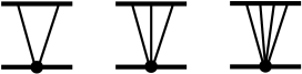
In this section we consider the dynamics at leading PM order and leading order in some additional perturbative correction. Our aim is to compute the perturbed scattering amplitude and Hamiltonian. In such a regime the test-particle limit encodes complete information about the dynamics at arbitrary mass ratio. This fact is obvious from the point of view of scattering amplitudes. Consider, for example, tidal corrections at leading PM order. These contributions are generated by the lowest order loop diagrams which induce classical scattering 3PM ; 3PMlong and enter at linear order in the tidal coefficient, corresponding to the “fan diagrams” depicted in Fig. 1. By definition, fan diagrams do not include matter propagators of the tidally distorted particle. More generally, we will henceforth refer to any diagram in which all matter propagators are on one side as a fan diagram. As discussed in 2PM ; 3PM ; 3PMlong ; 3PMFeynman , all fan diagrams are free from infrared divergences or iterations of lower order contributions. In the classical limit we are thus permitted to drop all recoil effects on the other particle, which can then be represented by a static background.
III.1 Lifting to Arbitrary Mass Ratio
At leading PM order the test-particle limit encodes sufficient data to reconstruct the perturbed scattering amplitude for arbitrary mass ratio in an arbitrary reference frame. To do this start we start with the test-particle amplitude and boost away from the rest frame by sending
| (15) |
Here and are the four-momenta of the scattering bodies in a boosted frame where . At the same time, we also continue away from the test-particle limit to accommodate arbitrary masses and .
Applying the replacement in Eq. (15), we derive the leading PM tidal correction to the scattering amplitude for arbitrary mass ratio and in a general frame
| (16) |
where the left-hand side of Eq. (16) is the amplitude for arbitrary mass ratio in a general frame and the right-hand side is the amplitude in the test-particle limit in the rest frame of the heavy body, as defined in Eq. (13). Here the prefactor accounts for proper non-relativistic normalization after applying the replacement in Eq. (15). Note that if both bodies are tidally deformed then one should sum over Eq. (16) with particle labels swapped.
This procedure similarly applies to the isotropic Hamiltonian,
| (17) |
where the left-hand side of Eq. (17) is the Hamiltonian for arbitrary mass ratio in an arbitrary frame and the right-hand side is the isotropic gauge test-particle Hamiltonian in the rest frame of the heavy body.
III.2 Fourier Transform
Eq. (16) is an explicit formula for the leading PM scattering amplitude of tidally interacting bodies at arbitrary mass ratio written in terms of the amplitude in the test-particle limit. According to Eq. (14) the latter is essentially the isotropic gauge Hamiltonian in the test-particle limit. Consequently, our only task is to map the test-particle Hamiltonian in Eq. (8) to isotropic coordinates. Typically, this is achieved by explicitly constructing a coordinate transformation from to , as we will do in Sec. IV. In this section, we derive a much simpler procedure applicable at the leading PM order.
Our basic idea is to take and Fourier transform to momentum space to obtain . As discussed at length in 2PM ; 3PM ; 3PMlong one can compute the scattering amplitude mediated by the tidal corrections, treating as a Feynman vertex. Crucially, at leading PM order, the contribution to the amplitude is exactly proportional to albeit evaluated at on-shell kinematics. For a scattering particle with momentum and momentum transfer , the on-shell condition implies that , which is subleading in classical counting and can thus be dropped. From Eq. (14) we also know that the amplitude is given by the isotropic gauge Hamiltonian, so
| (18) |
where the replacement drops quantum contributions which are irrelevant to the classical dynamics. We can then Fourier transform to obtain the isotropic Hamiltonian in position space, .
Conveniently, we can perform this procedure—Fourier transforming to momentum space, dropping terms that vanish on-shell, and Fourier transforming back to position space—in a single step. This is encapsulated by the replacement,
| (19) |
where the left- and right-hand sides are exactly equal up to terms that Fourier transform to objects proportional to which can be discarded on-shell. See Appendix A for details. Also, note that this replacement must be used with care: it can only be applied after first expanding an expression fully in and , since Fourier transform and multiplication do not commute.
III.3 Tidal Operators
Let us now utilize the tools derived above to compute the leading PM tidal corrections to the isotropic gauge Hamiltonian. We emphasize that our procedure is purely algebraic and thus implemented with ease. In particular, for a tidal operator given by a product of traces of matrices built from electric and magnetic Weyl, i.e. , we simply calculate using Eq. (23) and Eq. (29) below, plug into Eq. (8), and apply the replacement rule in Eq. (19) to derive the isotropic Hamiltonian at arbitrary mass ratio in Eq. (17). As we will see, this procedure yields closed form results for certain infinite classes of tidal operators. We have verified that our results can also be obtained by the method of Ref. Bini:2020flp , and that we agree with all results collected in the Appendix of Zvi_tidal up to the choice of normalization.
III.3.1 Kretschmann Scalar to a Power:
As a first trivial example let us consider a tidal operator given by the Kretschmann scalar to a power. Computing in Schwarzschild coordinates and plugging into Eq. (8), we obtain the test-particle Hamiltonian
| (20) |
which is automatically in isotropic form. Boosting to an arbitrary frame via Eq. (17), we obtain the isotropic Hamiltonian at arbitrary mass ratio,
| (21) |
For , this agrees with previous results Bini:2020flp ; PMGR ; PMtidal ; Kalin:2020lmz . Note the relative factor of in the normalization of the tidal coefficient here as compared to PMtidal .
III.3.2 Electric Weyl to a Power:
Next, consider a tidal operator given by the trace of a power of the electric Weyl tensor,
| (22) |
where at leading order in tidal coefficients, is defined as in Eq. (4) with an energy component equal to . The choice of coordinates for the metric will not affect our answer at leading PM order since need only be evaluated on the Newtonian background. The mixed index electric Weyl tensor at leading PM order is
| (23) |
and its eigenvalues are
| (24) |
See App. B for these expressions at all orders in the PM expansion. Thus the electric Weyl tensor to the power is
| (25) |
We then apply a binomial expansion and then eliminate via the replacement in Eq. (19). Resumming terms analytically, we obtain the test-particle Hamiltonian in isotropic gauge,
| (26) |
Applying Eq. (17), we derive a closed form expression for the isotropic Hamiltonian at arbitrary mass ratio,
| (27) | ||||
The case of agrees with Bini:2020flp ; PMGR ; PMtidal ; Kalin:2020lmz while agrees with Bini:2020flp . We can similarly compute arbitrary products of traces of electric Weyl, noting that due to the simple form of the eigenvalues a trace of any product can be reduced to products of and .
III.3.3 Magnetic Weyl to a Power:
We can repeat the same procedure for a tidal operator given by the trace of a power of magnetic Weyl,
| (28) |
where is the dual Weyl tensor. The mixed index magnetic Weyl tensor is
| (29) |
and its eigenvalues are
| (30) |
with expressions at all PM orders in App. B. Any trace of an odd power of will vanish. The tidal operator is then
| (31) |
Expanding and replacing via Eq. (19), we obtain
| (32) |
Again applying Eq. (17), we obtain
| (33) | ||||
The case of agrees with previous results Bini:2020flp ; PMGR ; PMtidal ; Kalin:2020lmz , and is consistent with the relation . Due to the simple form of the eigenvalues of magnetic Weyl, any product of its traces can be reduced to a single trace .
III.4 Beyond Schwarzschild
Our method for extracting kinematic data from the geodesic equation applies quite generally. The only prerequisite for this approach is that the leading perturbative correction arises from a fan diagram in which the matter propagators are only on one side. For the remainder of this section we study scenarios in which the tidal interactions may be absent but the system still has some small perturbative correction that deviates from a binary system of Schwarzschild black holes in general relativity.
In the examples below we will assume a static, spherically symmetric metric that is a function of some small perturbative parameter. Plugging into Eq. (6), we then expand to linear order in the perturbative coefficient. Applying the replacement in Eq. (19), we obtain the test-particle Hamiltonian in isotropic coordinates, from which we derive the associated scattering amplitude and Hamiltonian for arbitrary mass ratio via Eq. (16) and Eq. (17).
III.4.1 Higher Derivative Corrections
As a concrete example let us consider a modification to general relativity given by the leading higher derivative correction to graviton self-interactions,
| (34) |
It is clear that at linear order in and leading PM order this correction contributions via a fan diagram which is accounted for by the geodesic equation. In the presence of Eq. (34) the perturbed metric is Cai:2019npx
| (35) |
Next, we plug Eq. (35) into Eq. (5) and expand . Solving to linear order in , we derive the perturbed Hamiltonian,
| (36) |
where we have truncated to leading PM order. Transforming to isotropic gauge via Eq. (19) yields
| (37) |
We then boost to an arbitrary frame via Eq. (17) and sum over the exchange of bodies 1 and 2 since Eq. (34) generates contributions from fan diagrams as well as their flipped partners. We thus obtain
| (38) |
which agrees with known results in the PN Brandhuber:2019qpg ; Emond:2019crr and PM Cristofoli:2019ewu ; Zvi_tidal expansions.
III.4.2 Electric Charge
Another application of our approach is the scattering of electrically charged bodies. While this is obviously irrelevant to astrophysical black holes, we can still derive scattering amplitudes of more formal interest. To begin, we consider the interactions of a neutral body of mass and charge with an electrically charged body of mass and charge in the test-particle limit, . We can define a charge-to-mass ratio parameter
| (39) |
for which . We take to be perturbatively small, i.e. corresponding to a milli-charged body.
To compute the geodesic motion we use the Reissner-Nördstrom metric in standard coordinates where
| (40) |
We then expand the Hamiltonian up to linear order in the charge-to-mass ratio, , and solve the geodesic equation in Eq. (2) order by order in . At zeroth order in , is obtained by inserting the metric for an uncharged black hole in Schwarzschild coordinates into Eq. (5). Meanwhile, at first order we obtain
| (41) |
again truncating to leading PM order. Applying the replacement rule in Eq. (19), we trivially obtain the isotropic test-particle Hamiltonian
| (42) |
Boosting to a general frame and lifting to arbitrary mass ratio we obtain
| (43) |
which describes a neutral body interacting with a charged body at lowest order in the charge. The static limit of this expression agrees exactly with BjerrumBohr:2002sx ; Butt:2006gv ; Faller:2007sy ; Holstein:2008sy after including the charge-to-mass ratio as defined in Eq. (39). This result is trivially generalized to include multiple electric and magnetic charges simply by inserting the sum of all charges squared into .
III.4.3 Electric Charge and Higher Derivative Corrections
Last but not least, we consider the case of a neutral body interacting with a charged body in the presence of both tidal distortion and higher derivative corrections to the Einstein-Maxwell system,
| (46) | ||||
where the global prefactor characterizes the overall size of the perturbations. Here we have included tidal corrections on the neutral body, so the geodesic equation is Eq. (2) where and the tidal operator is
| (47) |
Of course, tidal interactions of this form can be eliminated with a field redefinition, but this fact will provide a useful consistency check of our final answer. Finally, let us define natural dimensionless coefficients,
| (48) |
for later convenience.
In this setup we consider the dynamics for arbitrary charge-to-mass ratio but treating the the overall scale of the higher derivative corrections as a small parameter. Since the coefficients modify the extremality condition for large black holes they are intimately linked to the weak gravity conjecture ArkaniHamed:2006dz , which mandates the instability of such objects to avoid remnant pathologies. Motivated by these connections, the linear in corrections to the Reissner-Nördstrom metric were computed in Kats:2006xp , and were later used to demonstrate the equivalence of the weak gravity conjecture to certain positivity conditions on black hole entropy Cheung:2018cwt ; Cheung:2019cwi that are valid in any tree-level ultraviolet completion of Eq. (46). The corrected metric from Kats:2006xp is
| (49) |
where the perturbation functions to leading PM order are
| (50) | ||||
We again expand the Hamiltonian as , this time inserting Eq. (47) into Eq. (2) for and solving order by order in . At zeroth order in we obtain the Hamiltonian for a test-particle in the Reissner-Nördstrom background while at linear order we find
| (51) | ||||
at leading PM order. Again applying Eq. (19), we obtain the isotropic gauge Hamiltonian in the test-particle limit,
| (52) |
Lifting to arbitrary mass ratio and inserting , we obtain
| (53) |
which describes the dynamics of a neutral and charged body interacting via higher derivative corrections. A similar exercise can be done in the presence of electric and magnetic charges using the perturbed metric computed in Cheung:2019cwi .
A useful consistency check of Eq. (53) comes from invariance of physical quantities under field redefinitions of the graviton in the effective field theory defined by Eq. (46). In particular, we consider a redefinition of the metric Cheung:2018cwt ,
| (54) |
which corresponds to a shift of the tidal coefficients by
| (55) | ||||
and a shift of the higher dimension operator coefficients by
| (56) | ||||
We then find that Eq. (53) is invariant under Eq. (55) and Eq. (56), as expected since the isotropic Hamiltonian is proportional to the physical scattering amplitude at leading PM order.
IV All Orders in
Test-particle dynamics can offer useful consistency checks for higher order PM calculations. In this section we present a prescription for analytically deriving the isotropic gauge Hamiltonian in the test particle limit for a general tidal moment at all PM orders. From this quantity we then derive closed form expressions for the corresponding scattering amplitudes at all PM orders.
IV.1 Diffeomorphism to Isotropic Coordinates
To begin, we apply a radius-dependent diffeomorphism to an initial metric of the form in Eq. (3). The transformed line element is
| (57) |
Any diffeomorphism of the metric will produce a new set of coordinates that automatically preserves the usual Poisson bracket structure of the corresponding phase space variables. Crucially, can be an implicit function of constants of motion such as the energy and the angular momentum , so we define
| (58) |
By construction, the nontrivial component of the diffeomorphism starts at linear order in the tidal coefficients so it only modifies tidal corrections to the Hamiltonian. For our purposes will be a polynomial and only a finite number of the coefficients will be nonzero. Note that since and are constants of motion, derivatives with respect to yield , where we define
| (59) |
i.e. derivatives do not act on or .
Earlier, we solved the geodesic equation in Eq. (2) to obtain the Hamiltonian at zeroth order in the tidal coefficients in Eq. (5). Since the tidal operator enters algebraically as a mass deformation, we can solve Eq. (2) at linear order in the tidal coefficient to obtain
| (60) |
Noting the implicit dependence in , we then decompose Eq. (60) as and expand to linear order in . Similar to before, any term entering with an explicit factor of can be simplified since any appearance of can be replaced with the point-particle Hamiltonian in the absence of tidal effects, . So concretely, the tidal operator should be evaluated as and the diffeomorphism functions should be evaluated as and .
While will in general have dependence we can simplify our calculation by using the isotropic coordinates in Eq. (9) for the initial metric before applying the diffeomorphism. We will assume this for the remainder of this section. By contrast, the tidal Hamiltonian has dependence even if the initial metric is in isotropic coordinates. Since is quite complicated we do not write it explicitly here, but the procedure for computing it is completely mechanical and described above.
In the final step, we solve for the coefficients of the diffeomorphism to exactly cancel all dependence in . We immediately find that is a polynomial in of finite degree, so only a finite number of terms are needed in the diffeomorphism in Eq. (58). Demanding that the coefficient of every positive power of is zero then produces a set of differential equations for the coefficients in Eq. (58). These equations can be solved analytically, yielding closed form expressions for , which turn out to be rational functions of the radius .111The constants of integration are fixed so that the coefficients do not blow up at large .
Inserting the solved-for diffeomorphism back into yields the tidal Hamiltonian in isotropic coordinates,
| (61) |
where and are defined in Eq. (58) and Eq. (59), and must be solved for to eliminate all dependence in . Explicit expressions for these quantities will be presented in the examples given below. We again emphasize that all components of the initial metric are evaluated in isotropic coordinates. Importantly, every step of this procedure can be performed at all PM orders.
Following the procedure described in Sec. II.2, we obtain the scattering amplitude in the test-particle limit,
| (62) | ||||
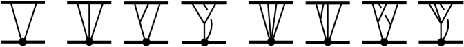
together with as defined in Eq. (13). These results are in the test-particle limit and at all orders in PM, and are equivalent to the resummation of the Feynman diagrams shown in Fig. 2.
It is straightforward to compute the scattering angle to arbitrarily high PM order from either the Hamiltonian or the scattering amplitude (see for example Vines:2018gqi ; 3PMlong ; B2B1 ; BDG2 ). We define the scattering angle as , where arises from minimal gravitational coupling and is the tidal correction at linear order. For we find
| (63) |
where and is the momentum at infinity. In all the examples we consider, we find that agrees when derived from versus , showing they are gauge equivalent.
IV.2 Examples
Next, let us apply the method just described to the following tidal moment operators:
| (64) |
Here we have defined where . To begin, we evaluate these operators on a background Schwarzschild metric in isotropic coordinates. See App. B for explicit expressions for electric and magnetic Weyl tensors at all PM orders. As noted earlier, since we are working at linear order in the tidal coefficients we can insert for the time component of the four-momentum that defines electric and magnetic Weyl. Our results in terms of are shown in Table. 1.
As discussed, by setting all dependence in to zero we derive a system of differential equations which can be solved to obtain the coefficients in Table. 3, where all coefficients not shown are vanishing. The solutions for are too cumbersome to display here but are included in the ancillary file. Note that the solutions for and are the same since the difference of these operators is the Kretschmann scalar, which is independent of .
From our results in Table. 1 and Table. 3, we assemble the isotropic test-particle Hamiltonian from Eq. (61) as well as the scattering amplitude from Eq. (62). The tidal corrections to the isotropic Hamiltonian and the scattering amplitude (modulo iterations) are summarized in Table. 3 and Table. 5. We emphasize again that these results are valid at all PM orders in the test-particle limit. However, we have verified that our expressions for and are consistent with the 3PM results of PMtidal in the test-particle limit.
Last but not least, as a check of our results we compute the tidal corrections to the scattering angle at several PM orders for both and and find that they agree, thus establishing their physical equivalence at that order. These scattering angles are presented in Table. 5. The Hamiltonian, amplitude, and scattering angle for are included in the ancillary file.
V Conclusions
Geodesic motion encodes all the kinematic data needed to reconstruct any scattering process mediated by fan diagrams, i.e., topologies in which only propagators of one of the bodies is present. In this work we have exploited this fact to derive the complete conservative dynamics—in the form of amplitudes and isotropic Hamiltonians—at leading PM order in various scenarios which deviate perturbatively from the minimal setup of a black hole binary system in general relativity. As we have demonstrated, our approach only entails simple algebraic manipulations and can be applied to a wide range of examples such as tidal operators and higher derivative corrections to gravitational or electromagnetic interactions. Furthermore, we have derived a method for computing the test-particle scattering amplitude to all PM orders, which could offer a useful check of higher PM calculations.
Acknowledgements. We thank Andreas Helset and Jan Steinhoff for comments on the manuscript. We thank Zvi Bern, Julio Parra-Martinez, Radu Roiban, Eric Sawyer and Chia-Hsien Shen for helpful discussions, especially regarding their concurrent work Zvi_tidal . C.C. and N.S. are supported by the DOE under grant no. DE-SC0011632 and by the Walter Burke Institute for Theoretical Physics. M.P.S. is supported by the Mani L. Bhaumik Institute for Theoretical Physics and David Saxon Presidential Term Chair in Physics. We used Mathematica Mathematica in combination with xAct xAct .
Appendix A Derivation of Eq. (19)
The replacement in Eq. (19) eliminates all dependence on the angular momentum in favor of powers of and . Its derivation is straightforward. To begin, consider the expression
| (65) |
where is precisely chosen so that the Fourier transform of Eq. (65) is zero at leading order in the classical limit. Our aim will be to derive .
The Fourier transform of the tensor is trivially obtained by taking derivatives of the Fourier transform of the scalar ,
| (66) | ||||
where the number of permutations in each summand is . Truncating all but leading order classical contribution of Eq. (65) effectively sets to zero. In the Fourier transform of Eq. (66), each derivative brings down a factor of . Therefore, the first term vanishes when all free indices are contracted into the momentum . Inserting Eq. (65) we find that
| (67) |
The solution to this equation is
| (68) |
which is shown simply by plugging into both sides of Eq. (67). Starting from the left-hand-side of Eq. (19) and eliminating all factors of via Eq. (65) given Eq. (68), we obtain
| (69) |
which correctly reproduces the right-hand-side of Eq. (19).
Appendix B Electric and Magnetic Weyl Tensors
Here we summarize the electric and magnetic Weyl tensors in isotropic coordinates at all orders in the PM expansion. The expressions below are written in terms of . The electric Weyl tensor is
| (70) |
and its eigenvalues are
| (71) |
The magnetic Weyl tensor is
| (72) |
and its eigenvalues are
| (73) |
References
- (1) H. Kawai, D. C. Lewellen and S. H. H. Tye, Nucl. Phys. B 269, 1 (1986); Z. Bern, L. J. Dixon, M. Perelstein and J. S. Rozowsky, Nucl. Phys. B 546, 423 (1999) [hep-th/9811140]; Z. Bern, J. J. M. Carrasco and H. Johansson, Phys. Rev. D 78, 085011 (2008) [arXiv:0805.3993 [hep-ph]]; Z. Bern, J. J. M. Carrasco and H. Johansson, Phys. Rev. Lett. 105, 061602 (2010) [arXiv:1004.0476 [hep-th]]; Z. Bern, J. J. Carrasco, M. Chiodaroli, H. Johansson and R. Roiban, arXiv:1909.01358 [hep-th].
- (2) Z. Bern, L. J. Dixon, D. C. Dunbar and D. A. Kosower, Nucl. Phys. B 425, 217 (1994) [hep-ph/9403226]; Z. Bern, L. J. Dixon, D. C. Dunbar and D. A. Kosower, Nucl. Phys. B 435, 59 (1995) [hep-ph/9409265]; Z. Bern, L. J. Dixon and D. A. Kosower, Nucl. Phys. B 513, 3 (1998) [hep-ph/9708239]; R. Britto, F. Cachazo and B. Feng, Nucl. Phys. B 725, 275 (2005) [hep-th/0412103]; Z. Bern, J. J. M. Carrasco, H. Johansson and D. A. Kosower, Phys. Rev. D 76, 125020 (2007) [arXiv:0705.1864 [hep-th]].
- (3) Y. Iwasaki, Prog. Theor. Phys. 46, 1587 (1971); Y. Iwasaki, Lett. Nuovo Cim. 1S2, 783 (1971) [Lett. Nuovo Cim. 1, 783 (1971)]; H. Okamura, T. Ohta, T. Kimura and K. Hiida, Prog. Theor. Phys. 50, 2066 (1973); D. Amati, M. Ciafaloni and G. Veneziano, Nucl. Phys. B 347, 550 (1990); J. F. Donoghue, Phys. Rev. Lett. 72, 2996 (1994) doi:10.1103/PhysRevLett.72.2996 [gr-qc/9310024]; J. F. Donoghue, Phys. Rev. D 50, 3874 (1994) doi:10.1103/PhysRevD.50.3874 [gr-qc/9405057]; N. E. J. Bjerrum-Bohr, J. F. Donoghue and B. R. Holstein, Phys. Rev. D 67, 084033 (2003) Erratum: [Phys. Rev. D 71, 069903 (2005)] doi:10.1103/PhysRevD.71.069903, 10.1103/PhysRevD.67.084033 [hep-th/0211072]; B. R. Holstein and A. Ross, arXiv:0802.0716 [hep-ph]; N. E. J. Bjerrum-Bohr, J. F. Donoghue and P. Vanhove, JHEP 1402, 111 (2014) doi:10.1007/JHEP02(2014)111 [arXiv:1309.0804 [hep-th]].
- (4) W. D. Goldberger and I. Z. Rothstein, Phys. Rev. D 73, 104029 (2006) doi:10.1103/PhysRevD.73.104029 [hep-th/0409156].
- (5) D. Neill and I. Z. Rothstein, Nucl. Phys. B 877, 177 (2013) doi:10.1016/j.nuclphysb.2013.09.007 [arXiv:1304.7263 [hep-th]].
- (6) C. Cheung, I. Z. Rothstein and M. P. Solon, Phys. Rev. Lett. 121, no. 25, 251101 (2018) doi:10.1103/PhysRevLett.121.251101 [arXiv:1808.02489 [hep-th]].
- (7) Z. Bern, C. Cheung, R. Roiban, C. H. Shen, M. P. Solon and M. Zeng, Phys. Rev. Lett. 122, no. 20, 201603 (2019) doi:10.1103/PhysRevLett.122.201603 [arXiv:1901.04424 [hep-th]].
- (8) Z. Bern, C. Cheung, R. Roiban, C. H. Shen, M. P. Solon and M. Zeng, JHEP 1910, 206 (2019) doi:10.1007/JHEP10(2019)206 [arXiv:1908.01493 [hep-th]].
- (9) C. Cheung and M. P. Solon, arXiv:2003.08351 [hep-th].
- (10) B. P. Abbott et al. [LIGO Scientific and Virgo Collaborations], Phys. Rev. Lett. 116, no. 6, 061102 (2016) [arXiv:1602.03837 [gr-qc]]; B. P. Abbott et al. [LIGO Scientific and Virgo Collaborations], Phys. Rev. Lett. 119, no. 16, 161101 (2017) [arXiv:1710.05832 [gr-qc]].
- (11) B. Bertotti, Nuovo Cimento 4:898–906 (1956). doi:10.1007/BF02746175; R. P. Kerr, I. Nuovo Cimento 13:469–491 (1959). doi:10.1007/BF02732767; B. Bertotti, J. F. Plebański, approximation”, Ann, Phys, 11:169–200 (1960). doi:10.1016/0003-4916(60)90132-9; M. Portilla, J. Phys. A 12, 1075 (1979). doi:10.1088/0305-4470/12/7/025; K. Westpfahl and M. Goller, Lett. Nuovo Cim. 26, 573 (1979). doi:10.1007/BF02817047; M. Portilla, J. Phys. A 13, 3677 (1980). doi:10.1088/0305-4470/13/12/017; L. Bel, T. Damour, N. Deruelle, J. Ibanez and J. Martin, Gen. Rel. Grav. 13, 963 (1981). doi:10.1007/BF00756073; K. Westpfahl, Fortschr. Phys., 33, 417 (1985); T. Ledvinka, G. Schaefer and J. Bicak, Phys. Rev. Lett. 100, 251101 (2008) doi:10.1103/PhysRevLett.100.251101 [arXiv:0807.0214 [gr-qc]]; T. Damour, Phys. Rev. D 94, no. 10, 104015 (2016) doi:10.1103/PhysRevD.94.104015 [arXiv:1609.00354 [gr-qc]]; T. Damour, Phys. Rev. D 97, no. 4, 044038 (2018) doi:10.1103/PhysRevD.97.044038 [arXiv:1710.10599 [gr-qc]]; A. Antonelli, A. Buonanno, J. Steinhoff, M. van de Meent and J. Vines, Phys. Rev. D 99, no.10, 104004 (2019) doi:10.1103/PhysRevD.99.104004 [arXiv:1901.07102 [gr-qc]]; G. Kälin, Z. Liu and R. A. Porto, [arXiv:2007.04977 [hep-th]].
- (12) J. Droste. Proc. Acad. Sc i. Amst. 19:447–455 (1916); A. Einstein, L. Infeld and B. Hoffmann, Annals Math. 39, 65 (1938). doi:10.2307/1968714; T. Ohta, H. Okamura, T. Kimura and K. Hiida, Prog. Theor. Phys. 50, 492 (1973). doi:10.1143/PTP.50.492; P. Jaranowski and G. Schäfer, Phys. Rev. D 57, 7274 (1998) Erratum: [Phys. Rev. D 63, 029902 (2001)] doi:10.1103/PhysRevD.57.7274, 10.1103/PhysRevD.63.029902 [gr-qc/9712075]; T. Damour, P. Jaranowski and G. Schäfer, Phys. Rev. D 62, 044024 (2000) doi:10.1103/PhysRevD.62.044024 [gr-qc/9912092]; L. Blanchet and G. Faye, Phys. Lett. A 271, 58 (2000) doi:10.1016/S0375-9601(00)00360-1 [gr-qc/0004009]; T. Damour, P. Jaranowski and G. Schäfer, Phys. Lett. B 513, 147 (2001) doi:10.1016/S0370-2693(01)00642-6 [gr-qc/0105038]; T. Damour, P. Jaranowski and G. Schäfer, Phys. Rev. D 89, no. 6, 064058 (2014) doi:10.1103/PhysRevD.89.064058 [arXiv:1401.4548 [gr-qc]]; P. Jaranowski and G. Schäfer, Phys. Rev. D 92, no. 12, 124043 (2015) doi:10.1103/PhysRevD.92.124043 [arXiv:1508.01016 [gr-qc]]; L. Bernard, L. Blanchet, A. Bohé, G. Faye and S. Marsat, Phys. Rev. D 93, no.8, 084037 (2016) doi:10.1103/PhysRevD.93.084037 [arXiv:1512.02876 [gr-qc]]; L. Bernard, L. Blanchet, A. Bohé, G. Faye and S. Marsat, Phys. Rev. D 95, no.4, 044026 (2017) doi:10.1103/PhysRevD.95.044026 [arXiv:1610.07934 [gr-qc]]; D. Bini and T. Damour, “Gravitational scattering of two black holes at the fourth post-Newtonian approximation,” Phys. Rev. D 96, no. 6, 064021 (2017) doi:10.1103/PhysRevD.96.064021 [arXiv:1706.06877 [gr-qc]]; L. Bernard, L. Blanchet, A. Bohé, G. Faye and S. Marsat, Phys. Rev. D 96, no.10, 104043 (2017) doi:10.1103/PhysRevD.96.104043 [arXiv:1706.08480 [gr-qc]]; T. Marchand, L. Bernard, L. Blanchet and G. Faye, Phys. Rev. D 97, no. 4, 044023 (2018) doi:10.1103/PhysRevD.97.044023 [arXiv:1707.09289 [gr-qc]]; L. Bernard, L. Blanchet, G. Faye and T. Marchand, Phys. Rev. D 97, no. 4, 044037 (2018) doi:10.1103/PhysRevD.97.044037 [arXiv:1711.00283 [gr-qc]].
- (13) F. Pretorius, Phys. Rev. Lett. 95, 121101 (2005) doi:10.1103/PhysRevLett.95.121101 [gr-qc/0507014]; M. Campanelli, C. O. Lousto, P. Marronetti and Y. Zlochower, Phys. Rev. Lett. 96, 111101 (2006) doi:10.1103/PhysRevLett.96.111101 [gr-qc/0511048]; J. G. Baker, J. Centrella, D. I. Choi, M. Koppitz and J. van Meter, Phys. Rev. Lett. 96, 111102 (2006) doi:10.1103/PhysRevLett.96.111102 [gr-qc/0511103].
- (14) A. Buonanno and T. Damour, Phys. Rev. D 59, 084006 (1999) [gr-qc/9811091]; A. Buonanno and T. Damour, Phys. Rev. D 62, 064015 (2000) [gr-qc/0001013].
- (15) Y. Mino, M. Sasaki and T. Tanaka, Phys. Rev. D 55, 3457 (1997) doi:10.1103/PhysRevD.55.3457 [gr-qc/9606018]; T. C. Quinn and R. M. Wald, Phys. Rev. D 56, 3381 (1997) doi:10.1103/PhysRevD.56.3381 [gr-qc/9610053].
- (16) J. B. Gilmore and A. Ross, Phys. Rev. D 78, 124021 (2008) doi:10.1103/PhysRevD.78.124021 [arXiv:0810.1328 [gr-qc]]; S. Foffa and R. Sturani, Phys. Rev. D 84, 044031 (2011) doi:10.1103/PhysRevD.84.044031 [arXiv:1104.1122 [gr-qc]]; S. Foffa, P. Mastrolia, R. Sturani and C. Sturm, Phys. Rev. D 95, no.10, 104009 (2017) doi:10.1103/PhysRevD.95.104009 [arXiv:1612.00482 [gr-qc]]; R. A. Porto and I. Z. Rothstein, Phys. Rev. D 96, no. 2, 024062 (2017) doi:10.1103/PhysRevD.96.024062 [arXiv:1703.06433 [gr-qc]]; S. Foffa, P. Mastrolia, R. Sturani, C. Sturm and W. J. Torres Bobadilla, Phys. Rev. Lett. 122, no. 24, 241605 (2019) doi:10.1103/PhysRevLett.122.241605 [arXiv:1902.10571 [gr-qc]]; J. Blümlein, A. Maier and P. Marquard, Phys. Lett. B 800, 135100 (2020) doi:10.1016/j.physletb.2019.135100 [arXiv:1902.11180 [gr-qc]]; S. Foffa, R. A. Porto, I. Rothstein and R. Sturani, Phys. Rev. D 100, no. 2, 024048 (2019) doi:10.1103/PhysRevD.100.024048 [arXiv:1903.05118 [gr-qc]]; J. Blümlein, A. Maier, P. Marquard and G. Schäfer, arXiv:2003.01692 [gr-qc]; J. Blümlein, A. Maier, P. Marquard and G. Schäfer, [arXiv:2003.07145 [gr-qc]].
- (17) A. Luna, R. Monteiro, I. Nicholson, D. O’Connell and C. D. White, “The double copy: Bremsstrahlung and accelerating black holes,” JHEP 1606, 023 (2016) doi:10.1007/JHEP06(2016)023 [arXiv:1603.05737 [hep-th]]; W. D. Goldberger and A. K. Ridgway, “Radiation and the classical double copy for color charges,” Phys. Rev. D 95, no. 12, 125010 (2017) doi:10.1103/PhysRevD.95.125010 [arXiv:1611.03493 [hep-th]]; W. D. Goldberger, S. G. Prabhu and J. O. Thompson, “Classical gluon and graviton radiation from the bi-adjoint scalar double copy,” Phys. Rev. D 96, no. 6, 065009 (2017) doi:10.1103/PhysRevD.96.065009 [arXiv:1705.09263 [hep-th]]; F. Cachazo and A. Guevara, JHEP 2002, 181 (2020) doi:10.1007/JHEP02(2020)181 [arXiv:1705.10262 [hep-th]]; W. D. Goldberger and A. K. Ridgway, “Bound states and the classical double copy,” Phys. Rev. D 97, no. 8, 085019 (2018) doi:10.1103/PhysRevD.97.085019 [arXiv:1711.09493 [hep-th]]; D. Chester, “Radiative double copy for Einstein-Yang-Mills theory,” Phys. Rev. D 97, no. 8, 084025 (2018) doi:10.1103/PhysRevD.97.084025 [arXiv:1712.08684 [hep-th]]; W. D. Goldberger, J. Li and S. G. Prabhu, “Spinning particles, axion radiation, and the classical double copy,” Phys. Rev. D 97, no. 10, 105018 (2018) doi:10.1103/PhysRevD.97.105018 [arXiv:1712.09250 [hep-th]]; J. Li and S. G. Prabhu, “Gravitational radiation from the classical spinning double copy,” Phys. Rev. D 97, no. 10, 105019 (2018) doi:10.1103/PhysRevD.97.105019 [arXiv:1803.02405 [hep-th]]; A. Laddha and A. Sen, Phys. Rev. D 100, no.2, 024009 (2019) doi:10.1103/PhysRevD.100.024009 [arXiv:1806.01872 [hep-th]]; N. E. J. Bjerrum-Bohr, P. H. Damgaard, G. Festuccia, L. Planté and P. Vanhove, Phys. Rev. Lett. 121, no. 17, 171601 (2018) [arXiv:1806.04920 [hep-th]]; C. H. Shen, “Gravitational radiation from color-kinematics duality,” JHEP 1811, 162 (2018) doi:10.1007/JHEP11(2018)162 [arXiv:1806.07388 [hep-th]]; J. Plefka, J. Steinhoff and W. Wormsbecher, Phys. Rev. D 99, no.2, 024021 (2019) doi:10.1103/PhysRevD.99.024021 [arXiv:1807.09859 [hep-th]]; B. Sahoo and A. Sen, JHEP 02, 086 (2019) doi:10.1007/JHEP02(2019)086 [arXiv:1808.03288 [hep-th]]; D. A. Kosower, B. Maybee and D. O’Connell, JHEP 1902, 137 (2019) [arXiv:1811.10950 [hep-th]]; M. Ciafaloni, D. Colferai and G. Veneziano, Phys. Rev. D 99, no.6, 066008 (2019) doi:10.1103/PhysRevD.99.066008 [arXiv:1812.08137 [hep-th]]; A. Koemans Collado, P. Di Vecchia and R. Russo, Phys. Rev. D 100, no. 6, 066028 (2019) doi:10.1103/PhysRevD.100.066028 [arXiv:1904.02667 [hep-th]]; A. Cristofoli, P. H. Damgaard, P. Di Vecchia and C. Heissenberg, [arXiv:2003.10274 [hep-th]]; L. de la Cruz, B. Maybee, D. O’Connell and A. Ross, [arXiv:2009.03842 [hep-th]]; G. Mogull, J. Plefka and J. Steinhoff, [arXiv:2010.02865 [hep-th]].
- (18) P. H. Damgaard, K. Haddad and A. Helset, JHEP 1911, 070 (2019) doi:10.1007/JHEP11(2019)070 [arXiv:1908.10308 [hep-ph]]; R. Aoude, K. Haddad and A. Helset, arXiv:2001.09164 [hep-th]; K. Haddad and A. Helset, arXiv:2005.13897 [hep-th].
- (19) S. Caron-Huot and Z. Zahraee, JHEP 1907, 179 (2019) doi:10.1007/JHEP07(2019)179 [arXiv:1810.04694 [hep-th]]; J. Parra-Martinez, M. S. Ruf and M. Zeng, [arXiv:2005.04236 [hep-th]].
- (20) J. M. Henn and B. Mistlberger, JHEP 1905, 023 (2019) doi:10.1007/JHEP05(2019)023 [arXiv:1902.07221 [hep-th]]; P. Di Vecchia, S. G. Naculich, R. Russo, G. Veneziano and C. D. White, arXiv:1911.11716 [hep-th]; Z. Bern, H. Ita, J. Parra-Martinez and M. S. Ruf, arXiv:2002.02459 [hep-th]; S. Abreu, F. Febres Cordero, H. Ita, M. Jaquier, B. Page, M. S. Ruf and V. Sotnikov, arXiv:2002.12374 [hep-th].
- (21) V. Vaidya, Phys. Rev. D 91, no. 2, 024017 (2015) doi:10.1103/PhysRevD.91.024017 [arXiv:1410.5348 [hep-th]]; A. Guevara, JHEP 1904, 033 (2019) doi:10.1007/JHEP04(2019)033 [arXiv:1706.02314 [hep-th]]; N. Arkani-Hamed, T. C. Huang and Y. t. Huang, arXiv:1709.04891 [hep-th]; J. Vines, Class. Quant. Grav. 35, no. 8, 084002 (2018) doi:10.1088/1361-6382/aaa3a8 [arXiv:1709.06016 [gr-qc]]; A. Guevara, A. Ochirov and J. Vines, JHEP 1909, 056 (2019) doi:10.1007/JHEP09(2019)056 [arXiv:1812.06895 [hep-th]]; M. Z. Chung, Y. T. Huang, J. W. Kim and S. Lee, JHEP 1904, 156 (2019) doi:10.1007/JHEP04(2019)156 [arXiv:1812.08752 [hep-th]]; Y. F. Bautista and A. Guevara, arXiv:1903.12419 [hep-th]; B. Maybee, D. O’Connell and J. Vines, JHEP 1912, 156 (2019) doi:10.1007/JHEP12(2019)156 [arXiv:1906.09260 [hep-th]]; A. Guevara, A. Ochirov and J. Vines, Phys. Rev. D 100, no. 10, 104024 (2019) doi:10.1103/PhysRevD.100.104024 [arXiv:1906.10071 [hep-th]]; N. Arkani-Hamed, Y. t. Huang and D. O’Connell, JHEP 2001, 046 (2020) doi:10.1007/JHEP01(2020)046 [arXiv:1906.10100 [hep-th]]; M. Z. Chung, Y. T. Huang and J. W. Kim, arXiv:1908.08463 [hep-th]; M. Z. Chung, Y. T. Huang and J. W. Kim, arXiv:1911.12775 [hep-th]; M. Levi, A. J. Mcleod and M. Von Hippel, [arXiv:2003.02827 [hep-th]]; M. Z. Chung, Y. t. Huang, J. W. Kim and S. Lee, arXiv:2003.06600 [hep-th]; M. Levi, A. J. Mcleod and M. Von Hippel, [arXiv:2003.07890 [hep-th]].
- (22) J. Vines, J. Steinhoff and A. Buonanno, Phys. Rev. D 99, no.6, 064054 (2019) doi:10.1103/PhysRevD.99.064054 [arXiv:1812.00956 [gr-qc]].
- (23) N. Siemonsen and J. Vines, Phys. Rev. D 101, no.6, 064066 (2020) doi:10.1103/PhysRevD.101.064066 [arXiv:1909.07361 [gr-qc]].
- (24) Z. Bern, A. Luna, R. Roiban, C. H. Shen and M. Zeng, arXiv:2005.03071 [hep-th].
- (25) A. Cristofoli, N. E. J. Bjerrum-Bohr, P. H. Damgaard and P. Vanhove, Phys. Rev. D 100, no. 8, 084040 (2019) doi:10.1103/PhysRevD.100.084040 [arXiv:1906.01579 [hep-th]].
- (26) G. Kälin and R. A. Porto, JHEP 2001, 072 (2020) doi:10.1007/JHEP01(2020)072 [arXiv:1910.03008 [hep-th]].
- (27) N. E. J. Bjerrum-Bohr, A. Cristofoli and P. H. Damgaard, JHEP 08, 038 (2020) doi:10.1007/JHEP08(2020)038 [arXiv:1910.09366 [hep-th]].
- (28) G. Kälin and R. A. Porto, JHEP 2002, 120 (2020) doi:10.1007/JHEP02(2020)120 [arXiv:1911.09130 [hep-th]].
- (29) P. Di Vecchia, C. Heissenberg, R. Russo and G. Veneziano, [arXiv:2008.12743 [hep-th]]; T. Damour, [arXiv:2010.01641 [gr-qc]].
- (30) A. Buonanno and B. Sathyaprakash, [arXiv:1410.7832 [gr-qc]].
- (31) T. Dietrich, T. Hinderer and A. Samajdar, [arXiv:2004.02527 [gr-qc]].
- (32) B. P. Abbott et al. [LIGO Scientific and Virgo Collaborations], Phys. Rev. Lett. 119, no. 16, 161101 (2017) doi:10.1103/PhysRevLett.119.161101 [arXiv:1710.05832 [gr-qc]].
- (33) B. P. Abbott et al. [LIGO Scientific and Virgo Collaborations], Astrophys. J. Lett. 892 (2020) L3 doi:10.3847/2041-8213/ab75f5 [arXiv:2001.01761 [astro-ph.HE]].
- (34) E. E. Flanagan and T. Hinderer, Phys. Rev. D 77, 021502 (2008) doi:10.1103/PhysRevD.77.021502 [arXiv:0709.1915 [astro-ph]].
- (35) C. Cutler, T. A. Apostolatos, L. Bildsten, L. S. Finn, E. E. Flanagan, D. Kennefick, D. M. Markovic, A. Ori, E. Poisson, G. J. Sussman and K. S. Thorne, Phys. Rev. Lett. 70, 2984-2987 (1993) doi:10.1103/PhysRevLett.70.2984 [arXiv:astro-ph/9208005 [astro-ph]]; C. Cutler and E. E. Flanagan, Phys. Rev. D 49, 2658-2697 (1994) doi:10.1103/PhysRevD.49.2658 [arXiv:gr-qc/9402014 [gr-qc]]; T. Hinderer, B. D. Lackey, R. N. Lang and J. S. Read, Phys. Rev. D 81, 123016 (2010) doi:10.1103/PhysRevD.81.123016 [arXiv:0911.3535 [astro-ph.HE]]; F. Pannarale, L. Rezzolla, F. Ohme and J. S. Read, Phys. Rev. D 84, 104017 (2011) doi:10.1103/PhysRevD.84.104017 [arXiv:1103.3526 [astro-ph.HE]]; T. Damour, A. Nagar and L. Villain, Phys. Rev. D 85, 123007 (2012) doi:10.1103/PhysRevD.85.123007 [arXiv:1203.4352 [gr-qc]]; M. Favata, Phys. Rev. Lett. 112, 101101 (2014) doi:10.1103/PhysRevLett.112.101101 [arXiv:1310.8288 [gr-qc]]; K. Yagi and N. Yunes, Phys. Rev. D 89, no.2, 021303 (2014) doi:10.1103/PhysRevD.89.021303 [arXiv:1310.8358 [gr-qc]]; B. D. Lackey and L. Wade, Phys. Rev. D 91, no.4, 043002 (2015) doi:10.1103/PhysRevD.91.043002 [arXiv:1410.8866 [gr-qc]]; L. Wade, J. D. Creighton, E. Ochsner, B. D. Lackey, B. F. Farr, T. B. Littenberg and V. Raymond, Phys. Rev. D 89, no.10, 103012 (2014) doi:10.1103/PhysRevD.89.103012 [arXiv:1402.5156 [gr-qc]]; K. Yagi and N. Yunes, Class. Quant. Grav. 34, no.1, 015006 (2017) doi:10.1088/1361-6382/34/1/015006 [arXiv:1608.06187 [gr-qc]]; S. E. Gralla, Class. Quant. Grav. 35, no.8, 085002 (2018) doi:10.1088/1361-6382/aab186 [arXiv:1710.11096 [gr-qc]]; A. Samajdar and T. Dietrich, Phys. Rev. D 98, no.12, 124030 (2018) doi:10.1103/PhysRevD.98.124030 [arXiv:1810.03936 [gr-qc]]; E. Poisson, Phys. Rev. D 101, no.10, 104028 (2020) doi:10.1103/PhysRevD.101.104028 [arXiv:2003.10427 [gr-qc]]; A. Le Tiec and M. Casals, [arXiv:2007.00214 [gr-qc]]; H. S. Chia, [arXiv:2010.07300 [gr-qc]].
- (36) M. Shibata, Phys. Rev. D 60, 104052 (1999) doi:10.1103/PhysRevD.60.104052 [arXiv:gr-qc/9908027 [gr-qc]]; L. Baiotti, B. Giacomazzo and L. Rezzolla, Phys. Rev. D 78, 084033 (2008) doi:10.1103/PhysRevD.78.084033 [arXiv:0804.0594 [gr-qc]]; S. Bernuzzi, A. Nagar, M. Thierfelder and B. Brugmann, Phys. Rev. D 86, 044030 (2012) doi:10.1103/PhysRevD.86.044030 [arXiv:1205.3403 [gr-qc]]; S. Bernuzzi, A. Nagar, T. Dietrich and T. Damour, Phys. Rev. Lett. 114, no.16, 161103 (2015) doi:10.1103/PhysRevLett.114.161103 [arXiv:1412.4553 [gr-qc]]; J. S. Read, C. Markakis, M. Shibata, K. Uryu, J. D. Creighton and J. L. Friedman, Phys. Rev. D 79, 124033 (2009) doi:10.1103/PhysRevD.79.124033 [arXiv:0901.3258 [gr-qc]]; L. Baiotti, T. Damour, B. Giacomazzo, A. Nagar and L. Rezzolla, Phys. Rev. Lett. 105, 261101 (2010) doi:10.1103/PhysRevLett.105.261101 [arXiv:1009.0521 [gr-qc]]; L. Baiotti, T. Damour, B. Giacomazzo, A. Nagar and L. Rezzolla, Phys. Rev. D 84, 024017 (2011) doi:10.1103/PhysRevD.84.024017 [arXiv:1103.3874 [gr-qc]]; B. D. Lackey, K. Kyutoku, M. Shibata, P. R. Brady and J. L. Friedman, Phys. Rev. D 85, 044061 (2012) doi:10.1103/PhysRevD.85.044061 [arXiv:1109.3402 [astro-ph.HE]].
- (37) T. Damour, M. Soffel and C. m. Xu, Phys. Rev. D 47, 3124-3135 (1993) doi:10.1103/PhysRevD.47.3124; T. Damour, M. Soffel and C. m. Xu, Phys. Rev. D 49, 618-635 (1994) doi:10.1103/PhysRevD.49.618; T. Hinderer, Astrophys. J. 677, 1216-1220 (2008) doi:10.1086/533487 [arXiv:0711.2420 [astro-ph]]; T. Damour and A. Nagar, Phys. Rev. D 80, 084035 (2009) doi:10.1103/PhysRevD.80.084035 [arXiv:0906.0096 [gr-qc]]; T. Binnington and E. Poisson, Phys. Rev. D 80, 084018 (2009) doi:10.1103/PhysRevD.80.084018 [arXiv:0906.1366 [gr-qc]]; J. E. Vines and E. E. Flanagan, Phys. Rev. D 88, 024046 (2013) doi:10.1103/PhysRevD.88.024046 [arXiv:1009.4919 [gr-qc]]; J. Vines, E. E. Flanagan and T. Hinderer, Phys. Rev. D 83, 084051 (2011) doi:10.1103/PhysRevD.83.084051 [arXiv:1101.1673 [gr-qc]]; Q. Henry, G. Faye and L. Blanchet, [arXiv:2005.13367 [gr-qc]]. Q. Henry, G. Faye and L. Blanchet, [arXiv:2009.12332 [gr-qc]].
- (38) J. Steinhoff, T. Hinderer, A. Buonanno and A. Taracchini, Phys. Rev. D 94, no.10, 104028 (2016) doi:10.1103/PhysRevD.94.104028 [arXiv:1608.01907 [gr-qc]].
- (39) Q. Henry, G. Faye and L. Blanchet, Phys. Rev. D 101, no.6, 064047 (2020) doi:10.1103/PhysRevD.101.064047 [arXiv:1912.01920 [gr-qc]].
- (40) D. Bini and T. Damour, Phys. Rev. D 90, no.12, 124037 (2014) doi:10.1103/PhysRevD.90.124037 [arXiv:1409.6933 [gr-qc]]; C. Kavanagh, A. C. Ottewill and B. Wardell, Phys. Rev. D 92, no.8, 084025 (2015) doi:10.1103/PhysRevD.92.084025 [arXiv:1503.02334 [gr-qc]]; P. Nolan, C. Kavanagh, S. R. Dolan, A. C. Ottewill, N. Warburton and B. Wardell, Phys. Rev. D 92, no.12, 123008 (2015) doi:10.1103/PhysRevD.92.123008 [arXiv:1505.04447 [gr-qc]].
- (41) T. Damour and A. Nagar, Phys. Rev. D 81, 084016 (2010) doi:10.1103/PhysRevD.81.084016 [arXiv:0911.5041 [gr-qc]]; D. Bini, T. Damour and G. Faye, Phys. Rev. D 85, 124034 (2012) doi:10.1103/PhysRevD.85.124034 [arXiv:1202.3565 [gr-qc]].
- (42) D. Bini, T. Damour and A. Geralico, Phys. Rev. D 101, no.4, 044039 (2020) doi:10.1103/PhysRevD.101.044039 [arXiv:2001.00352 [gr-qc]].
- (43) G. Kälin and R. A. Porto, arXiv:2006.01184 [hep-th].
- (44) C. Cheung and M. P. Solon, [arXiv:2006.06665 [hep-th]].
- (45) W. D. Goldberger and I. Z. Rothstein, [arXiv:2007.00731 [hep-th]].
- (46) K. Haddad and A. Helset, [arXiv:2008.04920 [hep-th]].
- (47) G. Kälin, Z. Liu and R. A. Porto, [arXiv:2008.06047 [hep-th]].
- (48) S. Endlich, V. Gorbenko, J. Huang and L. Senatore, JHEP 09, 122 (2017) doi:10.1007/JHEP09(2017)122 [arXiv:1704.01590 [gr-qc]].
- (49) V. Cardoso, M. Kimura, A. Maselli and L. Senatore, Phys. Rev. Lett. 121, no.25, 251105 (2018) doi:10.1103/PhysRevLett.121.251105 [arXiv:1808.08962 [gr-qc]].
- (50) N. Sennett, R. Brito, A. Buonanno, V. Gorbenko and L. Senatore, Phys. Rev. D 102, no.4, 044056 (2020) doi:10.1103/PhysRevD.102.044056 [arXiv:1912.09917 [gr-qc]].
- (51) B. S. Sathyaprakash, A. Buonanno, L. Lehner, C. Van Den Broeck, P. Ajith, A. Ghosh, K. Chatziioannou, P. Pani, M. Puerrer and S. Reddy, et al. [arXiv:1903.09221 [astro-ph.HE]].
- (52) A. Brandhuber and G. Travaglini, JHEP 01, 010 (2020) doi:10.1007/JHEP01(2020)010 [arXiv:1905.05657 [hep-th]].
- (53) W. T. Emond and N. Moynihan, JHEP 12, 019 (2019) doi:10.1007/JHEP12(2019)019 [arXiv:1905.08213 [hep-th]].
- (54) A. Cristofoli, Phys. Lett. B 800, 135095 (2020) doi:10.1016/j.physletb.2019.135095 [arXiv:1906.05209 [hep-th]].
- (55) S. Cai and K. D. Wang, [arXiv:1906.06850 [hep-th]].
- (56) D. Bini, T. Damour and A. Geralico, Phys. Rev. Lett. 123, no. 23, 231104 (2019) doi:10.1103/PhysRevLett.123.231104 [arXiv:1909.02375 [gr-qc]]; D. Bini, T. Damour and A. Geralico, arXiv:2003.11891 [gr-qc];
- (57) D. Bini, T. Damour and A. Geralico, arXiv:2004.05407 [gr-qc].
- (58) A. Antonelli, C. Kavanagh, M. Khalil, J. Steinhoff and J. Vines, Phys. Rev. Lett. 125, no.1, 011103 (2020) doi:10.1103/PhysRevLett.125.011103 [arXiv:2003.11391 [gr-qc]]. A. Antonelli, C. Kavanagh, M. Khalil, J. Steinhoff and J. Vines, [arXiv:2010.02018 [gr-qc]].
- (59) N. Wex and G. Schäfer, “Innermost stable orbits for coalescing binary systems of compact objects-a remark” Class. Quantum Grav. 10, 2729 (1993). http://stacks.iop.org/0264-9381/10/i=12/a=028
- (60) N. E. J. Bjerrum-Bohr, Phys. Rev. D 66, 084023 (2002) doi:10.1103/PhysRevD.66.084023 [arXiv:hep-th/0206236 [hep-th]].
- (61) M. S. Butt, Phys. Rev. D 74, 125007 (2006) doi:10.1103/PhysRevD.74.125007 [arXiv:gr-qc/0605137 [gr-qc]].
- (62) S. Faller, Phys. Rev. D 77, 124039 (2008) doi:10.1103/PhysRevD.77.124039 [arXiv:0708.1701 [hep-th]].
- (63) B. R. Holstein and A. Ross, [arXiv:0802.0717 [hep-ph]].
- (64) N. Arkani-Hamed, L. Motl, A. Nicolis and C. Vafa, JHEP 06, 060 (2007) doi:10.1088/1126-6708/2007/06/060 [arXiv:hep-th/0601001 [hep-th]].
- (65) Y. Kats, L. Motl and M. Padi, JHEP 12, 068 (2007) doi:10.1088/1126-6708/2007/12/068 [arXiv:hep-th/0606100 [hep-th]].
- (66) C. Cheung, J. Liu and G. N. Remmen, JHEP 10, 004 (2018) doi:10.1007/JHEP10(2018)004 [arXiv:1801.08546 [hep-th]].
- (67) C. Cheung, J. Liu and G. N. Remmen, Phys. Rev. D 100, no.4, 046003 (2019) doi:10.1103/PhysRevD.100.046003 [arXiv:1903.09156 [hep-th]].
- (68) T. Damour, [arXiv:1912.02139 [gr-qc]].
- (69) Wolfram Research, Inc., Mathematica, Version 12.0, Champaign, IL (2019).
- (70) Jose M. Martin-Garcia, et al. xAct: Efficient tensor computer algebra for the Wolfram Language. http://www.xact.es/
- (71) Z. Bern, J. Parra-Martinez, R. Roiban, E. Sawyer and C. H. Shen, ”Leading Nonlinear Tidal Deformations and Scattering Amplitudes,” to appear.