Abstract

We present the two-body Hamiltonian and associated eikonal phase, to leading post-Minkowskian order, for infinitely many tidal deformations described by operators with arbitrary powers of the curvature tensor. Scattering amplitudes in momentum and position space provide systematic complementary approaches. For the tidal operators quadratic in curvature, which describe the linear response to an external gravitational field, we work out the leading post-Minkowskian contributions using a basis of operators with arbitrary numbers of derivatives which are in one-to-one correspondence with the worldline multipole operators. Explicit examples are used to show that the same techniques apply to both bodies interacting tidally with a spinning particle, for which we find the leading contributions from quadratic in curvature tidal operators with an arbitrary number of derivatives, and to effective field theory extensions of general relativity. We also note that the leading post-Minkowskian order contributions from higher-dimension operators manifest double-copy relations. Finally, we comment on the structure of higher-order corrections.

1 Introduction

The remarkable discovery of gravitational waves by the LIGO and Virgo collaborations [1] has ushered in a new era of exploration that promises major new discoveries on black holes, neutron stars and perhaps even new basic insights into fundamental physics. Theoretical tools of increased precision, matching that of gravitational-wave signals not only from current detectors but also from proposed gravitational-wave observatories [2], are required.

The evolution of a compact binary and the ensuing gravitational-wave emission can be divided in three distinct phases — inspiral, merger and ring down — according to their underlying properties. The inspiral part of binary mergers, which is the subject of this paper, is analyzed through models such as the effective one-body (EOB) formalism [3]. The weak gravitational field during this phase makes it suitable for a perturbative approach and these models import information from post-Newtonian (PN) gravity [4, 5, 6, 7], as well as the self-force framework [8] and numerical relativity [9]. More recently, the post-Minkowskian (PM) expansion [10, 11, 12, 13, 14, 15, 16] has gained prominence due to its capture of the complete velocity dependence at fixed order in Newton’s constant. By exposing the analytic structure of each order, this expansion also offers new insight into features of gravitational perturbation theory, exposes hereto unexpected structure in certain observables, and may open a path to the resummation of perturbation theory in the classical limit. The PN, PM and self-force expansions provide important nontrivial cross checks in their overlapping regions of validity [13, 14, 7, 17]. For recent reviews see Refs. [18].

Over the years a close link between classical physics and scattering amplitudes has been developed [19, 20, 11, 12, 13, 15, 21] and led to a robust and powerful means for obtaining two-body Hamiltonians [11] and observables in the post-Minkowskian expansion. It was obtained by combining modern techniques, such as generalized unitarity [22], which emphasize gauge-invariant building blocks at all stages and build higher-order contributions from lower-order ones with effective field theory methods. This framework proved its effectiveness through the construction of the sought after two-body Hamiltonian at the third order in Newton’s constant [12, 13] and the identification of surprising simplicity in physical observables of interacting spinning black holes [23]. The scattering angle is of particular importance, as it provides a direct link [20] with the EOB framework [3] used to predict gravitational wave emission from compact binaries.

In this paper we investigate the effects of tidal deformations [24] on the conservative two-body Hamiltonian during the inspiral phase, focusing on their structure in the post-Minkowskian expansion. The tidal deformations offer a window into the equation of state of neutrons stars [25] and test our understanding of black holes [26, 27, 28, 21, 29, 30] and of possible exotic physics [31]. While tidal effects are expected to vanish for black holes in general relativity [32], they are of crucial importance for understanding the equation of state of neutron stars. These corrections are formally equivalent to fifth-order post-Newtonian effects [5], highlighting the importance of precision perturbative calculations.

Properties of extended bodies that relate to their finite size can be encoded in local-operator deformations of a point-particle theory by integrating out their internal degrees of freedom. The set of all possible tidal operators is constrained only by the symmetry properties of the fundamental theory, such as parity. We introduce our organization of tidal operators in close analogy with the case of electromagnetic susceptibilities. Indeed, not only is there a formal similarity between gauge theory and gravity, but the integrand of gravitational scattering amplitudes can be obtained directly from gauge theory using the double copy [33, 34]. For the relatively simple case of the leading-PM order contribution of a given tidal operator to scattering amplitudes, these relations follow from the factorization of the point-particle energy-momentum tensor and from the fact that the linearized Riemann tensor is a product of two gauge-theory field strengths. Thus, in analogy with the case of electromagnetic interactions of extended bodies, tidal operators may contain arbitrarily-high number of Riemann curvature tensors with an arbitrary number of derivatives.

Curvature-squared tidal operators, describing the linear response of an extended body to an external gravitational field, were recently classified in Ref. [30], where an expression for the two-body Hamiltonian and scattering angle at leading post-Minkowskian order was conjectured. Here we prove the conjecture for a basis of operators whose Wilson coefficients in the four-dimensional point-particle effective action are exactly the same as the worldline electric and magnetic tidal coefficients, related to the corresponding multipole Love numbers by factors of the typical scale of the body, see e.g. Ref. [5, 28, 25]. The lowest-order matrix elements of our tidal operators are, by construction, the same as the matrix elements of the worldline tidal operators. To establish the map beyond leading order it is necessary to compare physical quantities. At the next-to-leading order the contributions of low-derivative $R^{2}$ tidal operators to the two-body Hamiltonian and to the scattering angle were determined in Refs. [21, 29].

We also obtain the leading-order modifications of the two-body Hamiltonian and of the scattering angle due to tidal operators with arbitrarily-high number of Weyl tensors, which describe the nonlinear response of extended bodies to external gravitational field. As usual we organize the operators in terms of electric and magnetic-type components, $E$ and $B$, of the Riemann (or Weyl) tensor. The finite rank of these tensors leads to nontrivial relations between different operators, allowing us to express the contributions of $E^{n}$ and $B^{n}$-type operators for $n\geq 4$ in terms of those of products of simpler operators, thus reducing the number of independent structures.

While these relations appear mysterious for scattering amplitudes in momentum space, they are made manifest by Fourier-transforming the integral representation of the amplitude to position space. At any loop order, the transform decouples all integrals from each other. This observation allows us to write down closed-form expressions for amplitudes, two-body Hamiltonians and scattering angles generated by infinite families of operators. Beyond leading order the structure of tidally-deformed amplitudes is more complicated, but the momentum-space methods of Refs. [11, 12, 13, 21] can be applied systematically. Integration by parts methods [35] are especially powerful for the conservative two-body problem because in the potential region of loop integrals all relevant integrals are of single-scale type [36].

The methods we use to describe tidal operators apply equally well to deformations of a point-particle theory by any operators, including e.g. those arising in effective field theory extensions of General Relativity [37, 38, 39, 40]. We illustrate this point by working out the contributions of $R^{3}$ and $R^{4}$ and compare them with existing results. The two-body Hamiltonian and associated observables for a point-particle deformed by tidal operators interacting with a spinning particle can also be derived through similar methods. To leading PM order, only the single-graviton interaction of the spinning particle is relevant and it is captured by the stress tensors described in [41, 42, 23]. As an example, we find the leading spin-orbit contributions from $E^{2}$-type tidal operators with an arbitrary number of derivatives interacting with a spinning particle.

This paper organized as follows. In Sec. 2 we present a description of the operators encoding tidal deformations. In Sec. 3 we discuss the leading-order tidal contributions from $R^{2}$-type operators with an arbitrary number of derivatives. This section also demonstrate how to incorporate spin effects for the second body. We proceed to derive in Sec. 4 the leading contributions of various infinite classes of $R^{n}$-type tidal operators and also comment on their higher-order contributions. In Sec. 5 we discuss the application of our methods to the case of $R^{n}$ extensions of General Relativity. We present our conclusions in Sec. 6. An appendix gives the explicit results for the contributions of a collection of high-order tidal operators to the two-body Hamiltonian and the associate scattering amplitudes.

Note added: While this project was ongoing we became aware of concurrent work by Cheung, Shah and Solon [43] based on using the geodesic equation and containing some overlap on leading contributions to the two-body Hamiltonian from the $R^{n}$ tidal operators. In addition, the methods developed there determine the two-body Hamiltonian for a tidally-deformed test particle interacting with a Schwarzschild black hole, to all orders in the Schwarzschild radius of the latter. We are grateful for interesting and helpful discussions and sharing drafts.

2 Effective actions for tidal effects

2.1 Effective actions for post-Minkowskian potentials

In this work we study tidal or finite-size effects in the gravitational interactions of two massive extended bodies. They are encoded in a classical two-body Hamiltonian of the form

$$H(\bm{p},\bm{r})=\sqrt{\bm{p}^{2}+m_{1}^{2}}+\sqrt{\bm{p}^{2}+m_{2}^{2}}+V(\bm{p},\bm{r})\,,$$ (2.1)

and is extracted systematically, following the general approach introduced in [11], by matching QFT scattering amplitudes to a non-relativistic EFT. If the size of the two bodies is much smaller than their separation, non-analytic/long-distance classical potential has the form

$$V(\bm{p},\bm{r})\sim c_{i}(\bm{p})\,m\left(\frac{Gm}{|\bm{r}|}\right)^{i}\,,$$ (2.2)

where $m$ carries unit mass dimension and the momentum transfer $\bm{q}$, Fourier-conjugate to $\bm{r}$, is much smaller than the center of mass momentum $\bm{p}$. Such a conservative potential arises from integrating out gravitons with momenta $\ell$ in the potential region which has the scaling behavior

$$\ell=(\ell^{0},\bm{\ell})\sim(|\bm{q}||\bm{v}|,|\bm{q}|),$$ (2.3)

where $|\bm{v}|\sim\mathcal{O}\left(|\bm{p}|/m\right)$. Note that $Gm$ is of the order of the effective Schwarzschild radius of the particles $R_{s}$, so the classical expansion of the potential is an expansion in $R_{s}/|\bm{r}|$. If the separation of the two bodies can be of the same order as their typical size $R$, then the classical potential takes the form

$$V(\bm{p},\bm{r})\sim c_{i,k}(\bm{p})\,m\left(\frac{Gm}{|\bm{r}|}\right)^{i}\left(\frac{R}{|\bm{r}|}\right)^{k}\,.$$ (2.4)

For black holes $R\sim R_{s}$ so the size of terms with powers of $R$ is comparable to higher PM orders. For other bodies $R>R_{s}$ so the contribution should be bigger. For reference, neutrons stars have $R/R_{s}\sim 10$, and the sun has $R/R_{s}\sim 10^{5}$. In practice, it is convenient to always use $R_{s}/r$ as the expansion parameter so that the tidal effects just modify the coefficients in the usual PM potential, i.e. $c_{i,k}\sim\Delta c_{i+k}$.

From our point of view, the new scale $R_{s}$ is introduced by integrating out the degrees of freedom that describe the tidal dynamics of an extended body to yield a point-particle effective theory. In such an effective theory the finite size effects are encoded as higher-dimension operators ${\cal O}_{i}$ which are suppressed by powers of $R_{s}|\bm{q}|$. Their Wilson coefficients can be determined either by matching to the complete theory that includes the tidal degrees of freedom, or by comparing to experiment. A side effect of choosing $R_{s}$ instead of $R$ as the scale characterizing finite-size effects is that for less compact bodies the Wilson coefficients are not necessarily $\mathcal{O}(1)$. This approach was pioneered in the context of a worldline PN formalism in Ref. [5], and recently adapted to the PM framework in Ref. [29]. In the QFT language this approach has been recently used in Refs. [21, 30]. In section we provide a systematic treatment of such effective actions and write a basis of operators which simplifies the translation between QFT and worldline formalisms and makes the relation to familiar in-in observables manifest.

The cases that we focus on in this paper correspond to leading contributions from tidal or other operators. Although these operators first contribute to loop amplitudes, the determination of their leading-order contribution to the two-body potential is straightforward and formally given by inverting the Born relation between the scattering amplitude and the potential:

$$V_{\mathcal{O}}(\bm{p},\bm{r})=-\frac{1}{4E_{1}E_{2}}\int{d^{D-1}\bm{q}\over(2\pi)^{D-1}}e^{-i\bm{q}\cdot\bm{r}}\mathcal{M}_{\mathcal{O}}(\bm{p},\bm{q})\,.$$ (2.5)

Here $\mathcal{M}_{\mathcal{O}}$ is the leading-order four-scalar scattering amplitude with with a single insertion of $\mathcal{O}$, center of mass momentum $\bm{p}$, transferred momentum $\bm{q}$. In general the potential is gauge dependent and not unique. In the above equation we choose to expose the on-shell condition on $\bm{q}$ first such that $\bm{p}\cdot\bm{q}\simeq\mathcal{O}(\bm{q}^{2})\sim 0$. This naturally gives the potential in the isotropic gauge.

Alternatively, the effective two-body Hamiltonian can be constructed by matching its conservative observables — such as the conservative scattering angle, or the impulse and spin kick — or the closely-related eikonal phase [44],

$$\delta_{\mathcal{O}}(\bm{p},\bm{b}) =\frac{1}{4m_{1}m_{2}\sqrt{\sigma^{2}-1}}\int\frac{d^{D-2}\bm{q}}{(2\pi)^{D-2}}e^{-i\bm{b}\cdot\bm{q}}\mathcal{M}_{\mathcal{O}}(\bm{p},\bm{q})\,,$$ (2.6)

with the corresponding quantities in the complete theory. Here we use $-p_{i}=-m_{i}u_{i}$ as the incoming momenta of particle 1 and 2 and

$$\sigma\equiv\frac{p_{1}\cdot p_{2}}{m_{1}m_{2}}=u_{1}\cdot u_{2}\,.$$ (2.7)

In either case, the matching is carried out order by order in Newton’s constant $G$, that is order by order in the post-Minkowskian expansion. The relation between the eikonal and conservative observables holds also for the scattering of spinning particles. To leading nontrivial order, the effect of a composite operator ${\cal O}$ on the impulse and spin kick in the center-of-mass frame is

$$\Delta\bm{p}=-\nabla_{\bm{b}}\delta_{\mathcal{O}}(\bm{b})+\dots\,,\qquad\Delta\bm{S}_{i}=-\{{\bm{S}}_{i},\delta_{\mathcal{O}}(\bm{b})\}+\dots\,,$$ (2.8)

where the ellipsis stand for higher-order terms that depend on ${\cal O}$ and $\{\bullet,\bullet\}$ is the Poisson bracket. We expect that the all-order relation between the eikonal phase and conservative observables put forth in Ref. [23] holds in the presence of deformations by tidal and other composite operators. At leading order, the semiclassical approximation implies that the eikonal phase coincides with the radial action integrated over the scattering trajectory. We discuss this further in Section 3.3. The latter allows us to make contact with Ref. [28] in which tidal effects were computed using a classical worldline formalism for a subset of tidal operators.

Alternatively the matching can be performed by directly computing a physically meaningful quantity such as the conservative scattering angle, corresponding to the scattering with radiation reaction turned off; or the closely related eikonal phase. In either case matching is performed order by order in perturbation theory in Newton’s constant, $G$, that is order by order in the post-Minkowskian expansion.

$$\mathcal{M}_{\mathcal{O}}(\bm{q}) =|\bm{q}|^{A}\overline{\mathcal{M}}_{\mathcal{O}}\,,$$ (2.9)

$$V_{\mathcal{O}}(\bm{r}) =-\frac{1}{4E_{1}E_{2}}\frac{2^{A}\Gamma\left(\frac{1}{2}(D-1+A)\right)}{\pi^{(D-1)/2}\Gamma(-\frac{1}{2}A)}|\bm{r}|^{-A-(D-1)}\,\overline{\mathcal{M}}_{\mathcal{O}}\,,$$ (2.10)

$$\delta_{\mathcal{O}}(\bm{b}) =\frac{1}{4m_{1}m_{2}\sqrt{\sigma^{2}-1}}\frac{2^{A}\Gamma\left(\frac{1}{2}(D-2+A)\right)}{\pi^{(D-2)/2}\Gamma(-\frac{1}{2}A)}|\bm{b}|^{-A-(D-2)}\,\overline{\mathcal{M}}_{\mathcal{O}}\,,$$ (2.11)

where we have used the formula for the Fourier transform of a power

$$\int\frac{d^{D}\bm{q}}{(2\pi)^{D}}e^{-i\bm{x}\cdot\bm{q}}|\bm{q}|^{A}=\frac{2^{A}\Gamma\left(\frac{1}{2}(D+A)\right)}{\pi^{d/2}\Gamma(-\frac{1}{2}A)}|\bm{x}|^{-(A+D)}\,.$$ (2.12)

Here $A$ is power of the soft $q$ carried by the amplitude. For an operator with $n$ power of Riemann or Weyl tensors with $n_{\partial}$ derivatives acting on them, the leading contribution to the two-to-two scalar amplitude is

$$A=3n+n_{\partial}-3-2\epsilon(n-1),$$ (2.13)

where we use $D=4-2\epsilon$. For example, for the electric and magnetic operators $E^{2}$ and $B^{2}$ we will introduce shortly, $n=2$ and $n_{\partial}=0$ so $A=3-2\epsilon$, and every pair of derivatives acting of these increases $n_{\partial}$ and $A$ by two.

2.2 Effective actions for linear and non-linear tidal effects

We now explain how to parametrize the response of a general body to an external field and how this can be encoded in an effective action. We will discuss this in detail in the simpler case of electromagnetism, which will easily generalize to the gravitational case.

2.2.1 Tidal response in non-linear optics

The full non-linear response of a body to an external electric field $E_{i}$ is described by the induced electric dipole moment density $D_{i}$. In the rest frame of the body, it has a formal expansion in powers of the electric field [45]:

$$D_{i_{1}}(t,\bm{x}) =\chi^{(1)}_{i_{1}i_{2}}(t,\bm{x})E_{i_{2}}(t,\bm{x})+\chi^{(2)}_{i_{1}i_{2}i_{3}}(t,\bm{x})E_{i_{2}}(t,\bm{x})E_{i_{3}}(t,\bm{x})+\cdots\,.$$ (2.14)

The first term is the familiar linear response function; the subsequent terms encode the properties of the body in the susceptibility tensors, $\chi^{(n)}$, which are symmetric in their indices. Similarly, in the presence of a magnetic field $B_{i}$, one can write magnetic susceptibilities, as well as general susceptibilities capturing the response under a general electromagnetic field.

It is convenient to transform Eq. (2.14) to Fourier space, where it takes the form

$$D_{i_{1}}(-\omega_{1},-\bm{q}_{1}) =\chi^{(1)}_{i_{1}i_{2}}(\omega_{1},\bm{q}_{1};\omega_{2},\bm{q}_{2})E_{i_{2}}(\omega_{2},\bm{q}_{2})$$

$$\,\hskip 8.5359pt\hbox{}+\chi^{(2)}_{i_{1}i_{2}i_{3}}(\omega_{1},\bm{q}_{1};\omega_{2},\bm{q}_{2};\omega_{3},\bm{q}_{3})E_{i_{2}}(\omega_{2},\bm{q}_{2})E_{i_{3}}(\omega_{3},\bm{q}_{3})+\cdots\,.$$ (2.15)

Here we have adopted a generalized summation convention where repeated frequencies and momenta are integrated over, and the Fourier susceptibilities include energy-momentum-conservation delta functions

$$\chi^{(n-1)}_{i_{1}\cdots i_{n}}=\delta\left(\sum_{i}\omega_{i}\right)\delta\left(\sum_{i}\bm{q}_{i}\right)\tilde{\chi}^{(n-1)}_{i_{1}\cdots i_{n}}\,,$$ (2.16)

which account for the fact that the position-space product in Eq. (2.14) becomes a Fourier space convolution in Eq. (2.15).

The dipole density can be related to a generating function — or effective action — $S(E)$, via the usual response formula

$$D_{i_{1}}(-\omega_{1},-\bm{q}_{1})=\frac{\partial S(E)}{\partial E^{i_{1}}(\omega_{1},\bm{q}_{1})}\,.$$ (2.17)

The effective action, following from formally integrating Eq. (2.14), is given by

$$S(E) =\frac{1}{2}\chi^{(1)}_{i_{1}i_{2}}(\omega_{1},\bm{q}_{1};\omega_{2},\bm{q}_{2})E_{i_{1}}(\omega_{1},\bm{q}_{1})E_{i_{2}}(\omega_{2},\bm{q}_{2})$$

$$+\frac{1}{3}\chi^{(2)}_{i_{1}i_{2}i_{3}}(\omega_{1},\bm{q}_{1};\omega_{2},\bm{q}_{2};\omega_{3},\bm{q}_{3})E_{i_{1}}(\omega_{1},\bm{q}_{1})E_{i_{2}}(\omega_{2},\bm{q}_{2})E_{i_{3}}(\omega_{3},\bm{q}_{3})+\cdots\,.$$ (2.18)

This makes clear that the momentum space susceptibilities are completely symmetric tensors, as well as symmetric functions of all their arguments. $S(E)$ could be put in a form closer to an action by series expanding the susceptibilities and rewriting the powers of frequency and three-momenta as derivatives. For instance one can rewrite some terms in the expansion as follows

$$\left(\frac{\partial\chi^{(1)}_{i_{1}i_{2}}}{\partial\omega_{1}\partial\bm{q}_{2}^{j}}(0)\,\omega_{1}\bm{q}_{2}^{j}\right)E_{i_{1}}(\omega_{1},\bm{q}_{1})E_{i_{2}}(\omega_{2},\bm{q}_{2})\sim\left(\frac{\partial\chi^{(1)}_{i_{1}i_{2}}}{\partial\omega_{1}\partial\bm{q}_{2}^{j}}(0)\right)\partial_{t}E_{i_{1}}(t,\bm{x})\bm{\nabla}^{j}_{\bm{x}}E_{i_{2}}(t,\bm{x})\,.$$ (2.19)

Note that the expansion in the three momenta here simply corresponds to a multipole expansion of the electric fields.

So far we have been working in the rest frame of the object. The choice of a frame breaks manifest Lorentz invariance down to the rotations around the position of the object. We would like to covariantize the expressions above so that is they are valid in an arbitrary reference frame, in which the body moves with velocity $\bm{v}$. This can be done by considering the four-velocity of the object $u^{\mu}=\gamma(1,\bm{v})$, where $\gamma$ is the Lorentz factor. As is well known the electric field and magnetic fields in the rest frame of the body can be covariantly written as

$$E_{\mu}=F_{\mu\nu}u^{\nu}\,,\quad B_{\mu}=*F_{\mu\nu}u^{\nu}\,,$$ (2.20)

where $F_{\mu\nu}$ is the electromagnetic field strength, and $*F_{\mu\nu}$ its dual. Similarly, it is clear that any frequency and spatial momenta can be written as

$$\omega_{i}\rightarrow u\cdot q\equiv u^{\mu}q_{\mu}\,,\qquad\bm{q}_{i}\rightarrow(q^{\perp})_{\mu}\equiv P_{\mu\nu}q^{\nu}\,,$$ (2.21)

where we have introduced the four momentum of the field, $q_{i}^{\mu}$ and a projector,

$$P^{\mu\nu}=\eta^{\mu\nu}-u^{\mu}u^{\nu}\,,$$ (2.22)

which makes indices purely spatial in the rest frame of the object. Naively this covariantization requires adding components to the polarizabilities so that $\chi^{(n-1)}_{i_{1}\cdots i_{n}}\rightarrow\chi^{(n-1)}_{\mu_{1}\cdots\mu_{n}}$, and we can write

$$S(E) =\chi^{(1)}_{\mu_{1}\mu_{2}}(u\cdot q_{1},q^{\perp}_{1};u\cdot q_{2},q^{\perp}_{2})E_{\mu_{1}}(q_{1})E_{\mu_{2}}(q_{2})$$

$$+\chi^{(2)}_{\mu_{1}\mu_{2}\mu_{3}}(u\cdot q_{1},q^{\perp}_{1};u\cdot q_{2},q^{\perp}_{2},u\cdot q_{3},q^{\perp}_{3})E_{\mu_{1}}(q_{1})E_{\mu_{2}}(q_{2})E_{\mu_{3}}(q_{3})+\cdots\,,$$ (2.23)

due to the fact that $u^{\mu}E_{\mu}=u^{\mu}B_{\mu}=0$, which follows from the antisymmetry of the field strength.

The generating function written above describes the non-linear response of an arbitrary material, including those that violate rotational and Lorentz invariance. In the following we will be only interested in Lorentz-preserving effects, which impose addition constraints on the susceptibility tensors. Firstly, Lorentz invariance constrains the index structure of the susceptibility, which can only be carried by Lorentz-covariant tensors. If we impose parity, the only such tensors are the metric itself and the graviton momenta, so the tensor susceptibility must decompose in a set of scalar susceptibilities as follows

$$\chi^{(1)}_{\mu_{1}\mu_{2}} =\chi^{(1)}_{0}\,g_{\mu_{1}\mu_{2}}+\chi^{(1)}_{1}\,q^{\perp}_{1\,\mu_{1}}q^{\perp}_{2\,\mu_{2}}$$ (2.24)

$$\chi^{(2)}_{\mu_{1}\mu_{2}\mu_{3}} =\chi^{(2)}_{0}\,(g_{\mu_{1}\mu_{2}}q^{\perp}_{3\,\mu_{3}}+g_{\mu_{2}\mu_{3}}q^{\perp}_{1\,\mu_{1}}+g_{\mu_{3}\mu_{1}}q^{\perp}_{2\,\mu_{2}})\,,$$ (2.25)

$$\chi^{(3)}_{\mu_{1}\mu_{2}\mu_{3}\mu_{4}} =\chi^{(3)}_{0}\,g_{(\mu_{1}\mu_{2}}g_{\mu_{3}\mu_{4})}+\chi^{(3)}_{1}\,(g_{\mu_{1}\mu_{2}}q^{\perp}_{3\mu_{3}}q^{\perp}_{4\mu_{4}}+\text{perms})+\chi^{(3)}_{2}\,q^{\perp}_{1\mu_{1}}q^{\perp}_{2\mu_{2}}q^{\perp}_{3\mu_{3}}q^{\perp}_{4\mu_{4}}\,,$$ (2.26)

where in general each tensor structure must be summed over permutations which respect the symmetry $(\mu_{i}\leftrightarrow\mu_{j})$ while simultaneously swapping $q^{\perp}_{i}\leftrightarrow q^{\perp}_{j}$. Another consequence of Lorentz invariance is that the scalar susceptibilities only depend on Lorentz invariant combinations of momenta, so that

$$\chi^{(n-1)}_{a}(u\cdot q_{i};q^{\perp}_{i})\rightarrow\chi^{(n-1)}_{a}(u\cdot q_{i};q_{i}^{\perp}\cdot q_{j}^{\perp})\,.$$ (2.27)

Note that in the rest frame $q_{i}^{\perp}\cdot q_{j}^{\perp}=\bm{q}_{i}\cdot\bm{q}_{j}$.

2.2.2 Non-linear tidal response in gravity

It is now easy to generalize the tidal response for electromagnetism to its gravitational analog. In this case we start from the induced quadrupole moment, written in terms of the gravito-electric field

$$Q_{i_{1}j_{1}}(t,\bm{x}) =\chi^{(1)}_{i_{1}j_{1}i_{2}j_{2}}(t,\bm{x})E_{i_{2}j_{2}}(t,\bm{x})+\chi^{(2)}_{i_{1}j_{1}i_{2}j_{2}i_{3}j_{3}}(t,\bm{x})E_{i_{2}j_{2}}(t,\bm{x})E_{i_{3}j_{3}}(t,\bm{x})+\cdots\,,$$ (2.28)

where now the gravitational susceptibilities are more general tensors symmetric in each pair of $i$ and $j$ indices

$$\chi_{\cdots ij\cdots}=\chi_{\cdots ji\cdots}\,,\hskip 51.21504pt\chi_{\cdots i_{a}j_{a}\cdots i_{b}j_{b}\cdots}=\chi_{\cdots i_{b}j_{b}\cdots i_{a}j_{a}\cdots}\,.$$ (2.29)

In the rest frame of the object the electric field is related to the Weyl tensor as $E_{ij}=C_{0i0j}$. Similar expressions can be written for the response to a gravito-magnetic or to a mixed field.

All of these quantities can be covariantized by introducing

$$E_{\mu\nu}\equiv C_{\mu\alpha\nu\beta}u^{\alpha}u^{\beta},\qquad B_{\mu\nu}\equiv(*C)_{\mu\alpha\nu\beta}u^{\gamma}u^{\delta}\equiv\frac{1}{2}\epsilon_{\alpha\beta\gamma\mu}C^{\alpha\beta}_{\quad\delta\nu}u^{\gamma}u^{\delta},$$ (2.30)

where all indices are curved and the Levi-Civita tensor is defined as $\epsilon^{0123}=+1$. As in the electromagnetic case the following relations hold

$$E_{\mu\nu}u^{\nu}=0\,,\qquad B_{\mu\nu}u^{\nu}=0\,,$$ (2.31)

as well as

$$E_{\mu}{}^{\mu}=0\,,\qquad B_{\mu}{}^{\mu}=0\,,$$ (2.32)

where the first equality is a consequence of the tracelessness of the Weyl tensor. The corresponding generating function for tidal response is then simply

$$S_{\text{grav}}(E) =\chi^{(1)}_{\mu_{1}\nu_{1}\mu_{2}\nu_{2}}(u\cdot q_{1},Pq_{1};u\cdot q_{2},Pq_{2})\phi(p^{\prime})E^{\mu_{1}\nu_{1}}(q_{1})E^{\mu_{2}\nu_{2}}(q_{2})\phi(p)$$ (2.33)

$$\hskip 8.5359pt\hbox{}+\chi^{(2)}_{\mu_{1}\nu_{2}\mu_{2}\nu_{2}\mu_{3}\nu_{3}}(u\cdot q_{1},Pq_{1};u\cdot q_{2},Pq_{2},u\cdot q_{3},Pq_{3})\phi(p^{\prime})E^{\mu_{1}\nu_{1}}(q_{1})E^{\mu_{2}\nu_{2}}(q_{2})E^{\mu_{3}\nu_{3}}(q_{3})\phi(p)+\cdots$$

where, as above, a convolution over all momenta is implicit, and the covariant susceptibilities are traceless in each pair of $\mu,\nu$ indices $\eta^{\mu\nu}\chi_{\cdots\mu\nu\cdots}=0$. Once again, Lorentz invariance will further constraint the form of the susceptibility tensors in a way analogous to Eqs. (2.24)-(2.26).

2.2.3 From response to QFT effective actions

We now proceed to connect our discussion to a QFT effective action, focusing on the case of gravity; the electromagnetic case is completely analogous.

The connection can be easily made by interpreting the generating function, $S_{\text{grav}}(E)$ as the expectation value in a background field of an operator in a one-particle state $|p\rangle$ with four momentum $p=mu$, and zero spin. In second-quantized language the one-particle state is created by a scalar field, $\phi$, at infinity and

$$S_{\text{tidal}} =\chi^{(1)}_{\mu_{1}\mu_{2}}(u\cdot q_{1},q^{\perp}_{1};u\cdot q_{2},q^{\perp}_{2})\phi(p)E_{\mu_{1}}(q_{1})E_{\mu_{2}}(q_{2})\phi(p^{\prime})$$

$$+\chi^{(2)}_{\mu_{1}\mu_{2}\mu_{3}}(u\cdot q_{1},q^{\perp}_{1};u\cdot q_{2},q^{\perp}_{2},u\cdot q_{3},q^{\perp}_{3})\phi(p)E_{\mu_{1}}(q_{1})E_{\mu_{2}}(q_{2})E_{\mu_{3}}(q_{3})\phi(p^{\prime})+\cdots\,,$$ (2.34)

can be identified as the momentum-space effective action that encodes the response to the background field. Note that, in order to enforce momentum conservation, the Fourier-transformed susceptibilities must satisfy

$$\chi^{(n-1)}_{\mu_{1}\cdots\mu_{n}}=\delta\left(\sum_{i}q_{i}-q\right)\tilde{\chi}^{(n-1)}_{\mu_{1}\cdots\mu_{n}}\,,$$ (2.35)

where $q=-(p+p^{\prime})$. Note that the susceptibilities are initially only defined for $q=0$, so their covariantization requires an extension to $q\neq 0$. This does not affect the classical limit. As above, each term in the expansion of susceptibilities is encoded by a higher-dimension operator in the effective action, where now the factors of four-velocity $u$ can be identified with derivatives acting on the scalar field. For instance,

$$\partial_{\omega}^{2n}\chi^{(1)}_{\mu_{1}\nu_{1}\mu_{2}\nu_{2}}(0,0)[(u\cdot q_{1})^{2n}+(u\cdot q_{2})^{2n}]\phi(p^{\prime})E^{\mu_{1}\nu_{1}}(q_{1})E^{\mu_{2}\nu_{2}}(q_{2})\phi(p)$$

, $$\hskip 56.9055pt\leftrightarrow\partial_{\omega}^{2n}\chi^{(1)}_{\mu_{1}\nu_{1}\mu_{2}\nu_{2}}(0,0)\int d^{4}x\sqrt{-g}\,\frac{1}{m^{2n}}\phi E^{\mu_{1}\nu_{1}}\nabla_{(\rho_{1}\cdots\rho_{2n})}E^{\mu_{2}\nu_{2}}\nabla^{(\rho_{1}\cdots\rho_{2n})}\phi\,.$$ (2.36)

where the classical limit is implicit on the left-hand side. To write a generic operator appearing in this expansion it is convenient to introduce the combinations,

$${\hat{E}}_{\mu_{1}\mu_{2}\dots\mu_{n}} =\frac{i^{2}}{m^{2}}{\rm Sym}_{\mu_{1}\dots\mu_{n}}[\nabla_{\nu_{n}}\dots\nabla_{\nu_{3}}C_{\mu_{1}\alpha\mu_{2}\beta}{\hat{P}}_{\mu_{n}}^{\nu_{n}}\dots\hat{P}_{\mu_{3}}^{\nu_{3}}\nabla^{\alpha}\nabla^{\beta}\;]\,,$$

$${\hat{B}}_{\mu_{1}\mu_{2}\dots\mu_{n}} =\frac{i^{2}}{m^{2}}{\rm Sym}_{\mu_{1}\dots\mu_{n}}[\nabla_{\nu_{n}}\dots\nabla_{\nu_{3}}(*C)_{\mu_{1}\alpha\mu_{2}\beta}{\hat{P}}_{\mu_{n}}^{\nu_{n}}\dots\hat{P}_{\mu_{3}}^{\nu_{3}}\nabla^{\alpha}\nabla^{\beta}\;]\,,$$

$${\hat{E}}{}^{(l)}_{\mu_{1}\mu_{2}\dots\mu_{n}} =\frac{i^{m+2}}{m^{m+2}}{\rm Sym}_{\mu_{1}\dots\mu_{n}}[\nabla_{\nu_{n}}\dots\nabla_{\nu_{3}}\nabla^{\rho_{1}}\dots\nabla^{\rho_{l}}C_{\mu_{1}\alpha\mu_{2}\beta}{\hat{P}}_{\mu_{n}}^{\nu_{n}}\dots\hat{P}_{\mu_{3}}^{\nu_{3}}\nabla_{(\rho_{1}}\dots\nabla_{\rho_{l})}\nabla^{\alpha}\nabla^{\beta}\;]\,,$$

$${\hat{B}}{}^{(l)}_{\mu_{1}\mu_{2}\dots\mu_{n}} =\frac{i^{m+2}}{m^{m+2}}{\rm Sym}_{\mu_{1}\dots\mu_{n}}[\nabla_{\nu_{n}}\dots\nabla_{\nu_{3}}\nabla^{\rho_{1}}\dots\nabla^{\rho_{l}}(*C)_{\mu_{1}\alpha\mu_{2}\beta}{\hat{P}}_{\mu_{n}}^{\nu_{n}}\dots\hat{P}_{\mu_{3}}^{\nu_{3}}\nabla_{(\rho_{1}}\dots\nabla_{\rho_{l})}\nabla^{\alpha}\nabla^{\beta}\;]\,,$$ (2.37)

where all the derivatives on the right of the Weyl tensor act on the scalar field, and the position-space projector is

$${\hat{P}}_{\mu}^{\nu}=\frac{1}{m^{2}}(\partial_{\mu}\partial^{\nu}-\delta_{\mu}^{\nu}\partial^{2})\,.$$ (2.38)

The terms in the expansion that encode the most general linear response are then

$$S^{\text{QFT}}_{\text{tidal}}\big{|}_{\text{linear}}=m\int d^{4}x\sqrt{-g} \hphantom{+}\!\sum_{n=2}^{\infty}\sum_{l=0}^{\infty}(\mu^{(n,l)}\,\phi\hat{E}^{(l)}_{\mu_{1}\cdots\mu_{n}}\hat{E}^{(l)\,\mu_{1}\cdots\mu_{n}}\phi+\sigma^{(n,l)}\,\phi\hat{B}^{(l)}_{\mu_{1}\cdots\mu_{n}}\hat{B}^{(l)\,\mu_{1}\cdots\mu_{n}}\phi)\,$$ (2.39)

where the coefficients are related to the susceptibility as $\mu^{(n,l)}\sim(\partial_{\omega_{2}})^{l}(\partial_{q_{1}\cdot q_{2}})^{l}\chi^{(1)}_{0}(0;0)$, and the magnetic susceptibilities are related to $\sigma^{(n,l)}$ in a similar way. Operators like $\phi E_{\mu_{1}\mu_{2}}^{(l_{1})}E^{(l_{2})}{}^{\mu_{1}\mu_{2}}\phi$ with $l_{1}\neq l_{2}$ are related to operators with $l_{1}=l_{2}$ by integration by parts and use of scalar field equations of motion. We therefore can ignore them at this order. Similarly, the effective action

$$S^{\text{QFT}}_{\text{tidal}}\big{|}_{\text{non-linear}}=m\int d^{4}x\sqrt{-g} \hphantom{+}\!\sum_{n=2}^{\infty}(\rho_{e}^{(n)}\,\phi\hat{E}_{\mu_{1}}{}^{\mu_{2}}\hat{E}_{\mu_{2}}{}^{\mu_{3}}\cdots\hat{E}_{\mu_{n}}{}^{\mu_{1}}\phi+\rho_{m}^{(n)}\,\phi\hat{B}_{\mu_{1}}{}^{\mu_{2}}\hat{B}_{\mu_{2}}{}^{\mu_{3}}\cdots\hat{B}_{\mu_{n}}{}^{\mu_{1}}\phi)+\cdots$$ (2.40)

encodes part of the lowest-multipole time-independent non-linear response,

It is not difficult to translate the different terms in the response functions into a first quantized framework. This leads to a one-to-one relation between the higher-dimension operators in the QFT effective action and worldline operators. The factors of $u$ are identified with the four-velocity of the worldline $u^{\mu}=dx^{\mu}/{d\tau}$ and the factors of $(u\cdot\nabla)$ simply become derivatives with respect to the proper time $\tau$. Thus, the analog of the operators in the effective worldline action are

$$E_{\mu_{1}\mu_{2}\dots\mu_{n}} ={\rm Sym}_{\mu_{1}\mu_{2}\dots\mu_{n}}\left[P_{\mu_{3}}^{\nu_{3}}\dots P_{\mu_{n}}^{\nu_{n}}\nabla_{\nu_{3}}\dots\nabla_{\nu_{n}}C_{\mu_{1}\alpha\mu_{2}\beta}\right]u^{\alpha}u^{\beta}\,,$$ (2.41)

$$B_{\mu_{1}\mu_{2}\dots\mu_{n}} ={\rm Sym}_{\mu_{1}\mu_{2}\dots\mu_{n}}\left[P_{\mu_{3}}^{\nu_{3}}\dots P_{\mu_{n}}^{\nu_{n}}\nabla_{\nu_{3}}\dots\nabla_{\nu_{n}}(*C)_{\mu_{1}\alpha\mu_{2}\beta}\right]u^{\alpha}u^{\beta}\,,$$ (2.42)

$${E}^{(m)}_{\mu_{1}\dots\mu_{n}} =(u^{\alpha}\nabla_{\alpha})^{m}E_{\mu_{1}\dots\mu_{n}}=(\partial_{\tau})^{m}E_{\mu_{1}\dots\mu_{n}}\,,$$ (2.43)

$${B}^{(m)}_{\mu_{1}\dots\mu_{n}} =(u^{\alpha}\nabla_{\alpha})^{m}B_{\mu_{1}\dots\mu_{n}}=(\partial_{\tau})^{m}B_{\mu_{1}\dots\mu_{n}}\,,$$ (2.44)

where $P_{\mu\nu}=g_{\mu\nu}-u_{\mu}u_{\nu}$ is the $u$-orthogonal projector on the worldline. The effective action encoding the linear response are

$$S^{\text{worldline}}_{\text{tidal}}|_{\text{linear}}=\int d\tau \hphantom{+}\sum_{n=2}^{\infty}\sum_{l=0}^{\infty}\mu^{(n,l)}\,(E^{(l)}_{\mu_{1}\cdots\mu_{n}}E^{(l)\,\mu_{1}\cdots\mu_{n}}+\sigma^{(n,l)}\,B^{(l)}_{\mu_{1}\cdots\mu_{n}}B^{(l)\,\mu_{1}\cdots\mu_{n}})\,.$$ (2.45)

Note that here we use a different normalization than Ref. [28], the relation between our coefficients is $\mu^{(n,l)}_{\text{BDG}}=2l!\mu^{(n,l)}$ and $\sigma^{(n,l)}_{\text{BDG}}=2(l+1)!\sigma^{(n,l)}$. The non-linear response is captured by

$$S^{\text{worldline}}_{\text{tidal}}\big{|}_{\text{non-linear}}=\int d\tau \hphantom{+}\sum_{n=2}^{\infty}\rho_{e}^{(n)}\,E_{\mu_{1}}{}^{\mu_{2}}E_{\mu_{2}}{}^{\mu_{3}}\cdots E_{\mu_{n}}{}^{\mu_{1}}+\rho_{m}^{(n)}\,B_{\mu_{1}}{}^{\mu_{2}}B_{\mu_{2}}{}^{\mu_{3}}\cdots B_{\mu_{n}}{}^{\mu_{1}})+\cdots\,.$$ (2.46)

Thus, for a particle of mass $m_{i}$ described by the scalar field $\phi_{i}$, the correspondence between worldline operators and QFT Lagrangian operators is

$$\int d\tau E^{(l)}_{\mu_{1}\dots\mu_{n}}E^{(l)}{}^{\mu_{1}\dots\mu_{n}}\longleftrightarrow m_{i}\int d^{4}x\sqrt{-g}\phi_{i}{\hat{E}}^{(l)}_{\mu_{1}\dots\mu_{n}}{\hat{E}}^{(l)}{}^{\mu_{1}\dots\mu_{n}}\phi_{i}\,,$$ (2.47)

$$\int d\tau B^{(l)}_{\mu_{1}\dots\mu_{n}}B^{(l)}{}^{\mu_{1}\dots\mu_{n}}\longleftrightarrow m_{i}\int d^{4}x\sqrt{-g}\phi_{i}{\hat{B}}^{(l)}_{\mu_{1}\dots\mu_{n}}{\hat{B}}^{(l)}{}^{\mu_{1}\dots\mu_{n}}\phi_{i}\,.$$ (2.48)

The normalization of the QFT operators is fixed such that their four-point matrix elements in the classical limit reproduce the expectation value of the worldline operators, provided that the normalization of the asymptotic states is the same for both of them, i.e. it is a nonrelativistic normalization for the QFT states. One may similarly construct a correspondence between worldline and QFT operators with more factors of the Riemann tensor. For more details about the correspondence between QFT amplitudes and worldline matrix elements see e.g. Ref. [46].

2.2.4 Four dimensional relations

In any fixed dimension, the operators described above satisfy relations stemming from their finite number of components; thus they give an overcomplete description of the physics of extended bodies.

One class of relations follows from the the electric and magnetic fields being tensors of finite rank. Naively they have rank four, but because $E_{\mu\nu}u^{\nu}=B_{\mu\nu}u^{\nu}=0$ their rank is lowered to three. This is not a surprise: it is a consequence of the fact that $E_{\mu\nu}$ and $B_{\mu\nu}$ are the covariant versions of the purely spatial $E_{ij},B_{ij}$ in the rest frame. The simplest relation following from the finiteness of the ranks of $E$ and $B$ is

$$E_{[\mu_{1}}{}^{\mu_{2}}E_{\mu_{2}}{}^{\mu_{3}}E_{\mu_{3}}{}^{\mu_{4}}E_{\mu_{4}]}{}^{\mu_{1}}=0\,,$$ (2.49)

which, together with the tracelessness of $E$, implies that $E^{4}=1/2(E^{2})^{2}$. More generally, relations can be found which involve mixed powers of the electric and magnetic fields. For operators with no derivatives all such relations can be generated by evaluating the following determinant as a formal power series

$$\text{det}[1+t(E+rB)]=\sum_{i=2}^{\infty}\sum_{j=0}^{i}R_{i,j}t^{i}r^{j}\,.$$ (2.50)

The rank-three property of an arbitrary combination of $E$ and $B$ implies that $R_{i\geq 4,j}=0$. A sample of such relations is

$$2^{3}R_{4,0} =(E^{2})^{2}-2(E^{4})=0\,,$$

$$2^{2}R_{4,2} =2(EB)^{2}+(B^{2})(E^{2})-2(EBEB)-4(E^{2}B^{2})=0\,,$$

$$5R_{5,0} =(E^{5})-\frac{5}{6}(E^{2})(E^{3})=0\,,$$

$$6R_{5,2} =6(E^{2}BEB)+6(E^{3}B^{2})-(B^{2})(E^{3})-3(E^{2})(EB^{2})=0\,,$$

$$2R_{5,4} =2(EB^{4})-(B^{2})(EB^{2})=0\,,$$ (2.51)

as well as the ones that follow by interchanging $E$ and $B$. Here the round parenthesis denote the matrix trace,

$$({\cal O})\equiv{\rm Tr}[{\cal O}]\,.$$ (2.52)

Recursively solving them implies that any operator of the form $(E^{n\geq 4})$ can be written as a polynomial in $E^{2}$ and $E^{3}$ as follows

$$(E^{n}) =n\sum_{2p+3q=n}\frac{1}{2^{p}3^{q}}\,\frac{\Gamma(p+q)}{\Gamma(p+1)\Gamma(q+1)}(E^{2})^{p}\;(E^{3})^{q}\,.$$ (2.53)

A similar relation holds for $(B^{2n})$, while $(B^{2n+1})=0$ in a parity-invariant theory such as GR.

Another class of relations follows from the vanishing of the Gram determinants of any five or more four-momenta. They imply that certain terms in the power series expansion of susceptibilities are not linearly independent. For instance,

$$\text{det}(v_{i}\cdot v_{j})=0\quad\text{with}\quad v_{i}\subset\{p_{1},p_{2},q_{1},q_{2},q_{3}\}\,.$$ (2.54)

A final class of relations, which we will not detail any further, follows from the over-antisymmetrization of indices of both derivatives and $E$ or $B$.

An exhaustive enumeration of the $E^{2}$- and $B^{2}$-type operators was carried out in Ref. [30], using Hilbert series techniques [48], which automatically eliminate the redundancies described here. In contrast, we will not make an attempt to eliminate all redundant operators, but rather use their relations as a check on our framework and calculations.

3 Leading order $E^{2}$ and $B^{2}$ tidal effects

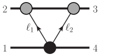
Figure 1: The generalized cut for leading-order contributions to $E^{2}$- or $B^{2}$-type tidal operators. Each blob is an on-shell amplitude, which in this case is local. Each exposed line is taken to be on shell and the blobs represent tree amplitudes. The dark blob contains an insertion of an $E^{2}$- or $B^{2}$-type higher-dimension operator with an arbitrary number of additional derivatives. The external momenta are all outgoing and the arrows indicated the direction of graviton momenta.

In this section we discuss the leading-order contribution of the two-graviton tidal operators constructed in Section 2. The analysis parallels to some extent that of Ref. [30], with the main difference being the choice of operator basis. Our choice aligns with the worldline approach [5, 28] making it straightforward to compare Love numbers. We also evaluate all integrals providing a proof of the results with arbitrary numbers of derivatives. Here we work in an amplitudes-based approach following Refs. [11, 12, 13, 21].

3.1 Constructing integrands

The first task is to write down a scattering amplitude from which classical scattering angles and Hamiltonians can be extracted. To obtain the integrand we use the generalized unitarity method [22]. In this method, the integrand is constructed from the generalized unitarity cut which we define to be

$$\mathcal{C}\equiv\sum_{\rm states}\mathcal{M}^{\rm tree}_{(1)}\mathcal{M}^{\rm tree}_{(2)}\mathcal{M}^{\rm tree}_{(3)}\cdots\mathcal{M}^{\rm tree}_{(m)}\,,$$ (3.1)

where the $\mathcal{M}^{\rm tree}_{(i)}$ are tree amplitudes, some of which can have operator insertion. As a simple example, Fig. 1 displays the unitarity cut containing the leading-order effect of an $R^{2}$ tidal operator.

In general, the cuts that can contribute to the conservative classical Hamiltonian satisfy some simple rules. The first is that generalized unitarity cuts must separate the two matter lines to opposite sides of a cut, which follows from the fact we are interested only in long-range interactions. Another general rule is that every independent loop must have at least one cut matter line, so the energy is restricted to a matter residue. Any contribution with a graviton propagator attached to the same matter line also does not contribute to the conservative classical part. Further details are found in Ref. [13].

In constructing the amplitude integrand we may immediately expand in soft-graviton momenta, since each power of graviton momentum effectively carries an additional power of $\hbar$ and is quantum suppressed. This expansion can be carries out either on at the level of the input tree amplitudes or after assembling the cuts. The order to which a give term needs to be expanded is dictated by simple counting rules. Terms with too high a scaling in the graviton momenta are dropped. For example, at one-loop for the case without tidal or other higher-dimension operators this implies that any term in a diagram numerator with more than a single power of loop momentum in the numerators yields only quantum-mechanical contributions; some terms require fewer loop-momentum factors. In the presence of higher-dimension operators, the leading classical contributions can have higher powers of loop momentum dictated simply by the number of extra derivatives in the operator compared to to the usual two derivative minimal coupling; the extra implicit powers of $\hbar$ are made up by the coefficient so the entire expression corresponds to a classical result.

In general to sew the trees together into generalized cuts one should use physical-state projectors which depend on null reference momenta

$$\mathbb{P}^{\mu\nu\rho\sigma}=\sum_{\rm states}{\varepsilon}^{\mu\nu}(-p){\varepsilon}^{\rho\sigma}(p)=\frac{1}{2}\Bigl{(}\mathbb{P}^{\mu\rho}\mathbb{P}^{\nu\sigma}+\mathbb{P}^{\mu\rho}\mathbb{P}^{\nu\sigma}\Bigr{)}-\frac{1}{D-2}\mathbb{P}^{\mu\nu}\mathbb{P}^{\rho\sigma}\,,$$ (3.2)

where $\mathbb{P}^{\mu\rho}=\eta^{\mu\rho}-(n^{\mu}p^{\rho}+n^{\rho}p^{\mu})/(n\cdot p)$ and $n^{\mu}$ is the null reference momentum. However, the reference momenta will drop out if the seed amplitudes are manifestly transverse. In fact, one can always arrange for such terms to automatically drop out [49].

Alternatively, we can also use four-dimensional helicity states to sew gravitons across unitarity cuts. In general, some caution is required in the presence of infrared or ultraviolet singularites, although at least through third post-Minkowskian order helicity methods have been shown to correctly capture all contributions [13]. For cases without non-trivial infrared or ultraviolet divergences , we can straightforwardly apply four-dimensional methods. In our cases, the above $D$-dimensional sewing is simple enough so we will not use four-dimensional helicities here.

Finally, the information from multiple generalized cuts must be merged into a single expression. This can either be accomplished at the level of the integrand or after integration. For leading tidal coefficients, effectively only a single cut contributes, so merging information from the cuts is trivial.

3.1.1 Simplifications from leading classical order

The on-shell amplitudes in the unitarity cut simplifies dramatically if we are only interested at leading classical order. Because there is no enhancement from iteration, any terms beyond the leading order in graviton momenta are quantum mechanical and can thus be ignored. For example, consider a three-point scalar-graviton-scalar amplitude at tree level

$${\cal M}_{3}(\phi(p),h(\ell),\phi(p^{\prime}))=-\kappa p^{\mu}p^{\nu}\varepsilon_{\mu\nu}(\ell)\,,$$ (3.3)

where $\kappa$ is related to Newton’s constant by $\kappa^{2}=32\pi G$. For any of the three-point amplitudes inserted in Fig. 1, we can replace the scalar momenta $p$ by the external momentum $p_{2}$ at leading classical order. Physically this implies that we ignore all back reaction on the particle 2, so all three-point amplitudes in Fig. 1 are approximately the same.

For the amplitude with higher-dimension operator, it suffices to use linearized version of the curvature operators. Expanding the metric in the usual way, $g_{\mu\nu}=\eta_{\mu\nu}+\kappa h_{\mu\nu}$, we find the Weyl tensor to leading order is

$$C_{\mu\nu\rho\sigma}=-2\kappa\partial_{[\mu|}\partial_{[\rho}h_{\sigma]|\nu]}+{\cal O}(\kappa^{2},\Box h)\,.$$ (3.4)

In deriving this expression we have also dropped terms proportional to the equations of motion for the graviton; this is because they do not contribute to the on-shell matrix elements necessary for the evaluation of the leading-order amplitude. The linearized Weyl tensor in momentum space then reads

$$C^{\rm lin}_{\mu\nu\rho\sigma}(\ell) \equiv\frac{\kappa}{2}\left[\ell_{\mu}\ell_{\rho}\,\varepsilon(\ell)_{\nu\sigma}-\ell_{\nu}\ell_{\rho}\,\varepsilon(\ell)_{\mu\sigma}-\ell_{\mu}\ell_{\sigma}\,\varepsilon(\ell)_{\nu\rho}+\ell_{\nu}\ell_{\sigma}\,\varepsilon(\ell)_{\mu\rho}\right].$$ (3.5)

The linearized Weyl tensor can be written a form that manifests the double copy in terms of two gauge-theory field strengths

$$C^{\rm lin}_{\mu\nu\rho\sigma}(\ell)=\frac{\kappa}{2}F^{\rm lin}_{\mu\nu}(\ell)F^{\rm lin}_{\rho\sigma}(\ell)\,,$$ (3.6)

where

$$F^{\rm lin}_{\mu\nu\rho\sigma}(\ell)\equiv\ell_{\mu}\varepsilon(\ell)_{\nu}-\ell_{\nu}\varepsilon(\ell)_{\mu}\,,$$ (3.7)

and we identify the graviton polarization tensor as $\varepsilon(\ell)_{\nu\sigma}=\varepsilon(\ell)_{\nu}\varepsilon(\ell)_{\sigma}$. This simple example of a double-copy relation [33, 34], which is trivial at the linearized level, then implies that the leading-order amplitudes for tidal operators display double-copy relations. The gauge invariance is manifest.

To make the gravitational coupling manifest in all equations, we will extract all factors of $\kappa$ from the building blocks of amplitudes. The linearized electric and magnetic components of the linearized Weyl tensor (3.5) follow from Eq. (2.30)

$${\cal E}_{\mu_{1}\mu_{2}}(\ell,p)=\frac{1}{2m^{2}}\left[\ell_{\mu_{1}}\ell_{\mu_{2}}(p\cdot\varepsilon(\ell)\cdot p)-(p\cdot\ell)\left(\ell_{\mu_{1}}\varepsilon(\ell)_{\mu_{2}\rho}p^{\rho}+\ell_{\mu_{2}}\varepsilon(\ell)_{\mu_{1}\rho}p^{\rho}\right)+\varepsilon(\ell)_{\mu_{1}\mu_{2}}(p\cdot\ell)^{2}\right],$$ (3.8)

$${\cal B}_{\mu_{1}\mu_{2}}(\ell,p)=\frac{1}{4m^{2}}\epsilon_{\alpha\beta\gamma\mu}\left[(p\cdot\ell)\,(\ell^{\alpha}\varepsilon(\ell)^{\beta}_{\,\;\mu_{2}}-\ell^{\beta}\varepsilon(\ell)^{\alpha}_{\,\;\mu_{2}})+\ell^{\beta}\ell_{\mu_{2}}(p\cdot\varepsilon(\ell))^{\alpha}-\ell^{\alpha}\ell_{\mu_{2}}(p\cdot\varepsilon(\ell))^{\beta}\right],$$ (3.9)

where the particle momentum and its four-velocity are related in the usual way, $p_{\mu}=mu_{\mu}$. It is then straightforward to assemble the amplitude with insertions of a higher-dimension operator from above formulae.

In general to sew trees into generalized cuts one should use physical-state projectors which depend on null reference momenta. However, for the leading-order contributions that we will mostly be studying here, the terms containing dependence on the reference momentum automatically drop out because they are contracted into manifestly gauge-invariant (transverse) quantities. Effectively, we can use the numerator of the de Donder gauge propagator,

$$\mathbb{P}^{\mu\nu\rho\sigma}=\sum_{\rm states}{\varepsilon}^{\mu\nu}(-p){\varepsilon}^{\rho\sigma}(p)\rightarrow\frac{1}{2}\Bigl{(}\eta^{\mu\rho}\eta^{\nu\sigma}+\eta^{\mu\rho}\eta^{\nu\sigma}\Bigr{)}-\frac{1}{D-2}\eta^{\mu\nu}\eta^{\rho\sigma}\,,$$ (3.10)

to sew gravitons across cuts. Combining the projector with the three-point amplitude in Eq. (3.3) at leading classical order, effectively turns the graviton polarization tensors of the higher-dimension operator into

$$\varepsilon_{\mu\nu}(\ell)\rightarrow T_{\mu\nu}(p_{2})=\left(p_{2,\mu}p_{2,\nu}-\frac{m_{2}^{2}}{D_{s}-2}\eta_{\mu\nu}\right)\,.$$ (3.11)

Crucially the result is independent of the loop momentum, implying that the sewing automatically imposes Bose symmetry for the gravitons of the higher-dimension operator. As we will outline in Sec. 4, this no longer holds beyond leading order where back-reaction becomes important. For example, at next-to-leading order pairs of the stress tensor in Eq. (3.3) can source a single graviton, acting as a sort of “impurity”, which may be interpreted as the first correction to the gravitational field of a free particle towards that of a Schwarzschild black hole.

The discussion above can be extended to include the leading-order scattering of scalars deformed by higher-dimension operators off higher-spin particles described the Lagrangian in Ref. [23]. For a generic spinning body the stress tensor is

$${\cal M}_{3}(\phi_{s}(p),h(\ell),\phi_{s}(p^{\prime})) =-\kappa\,V_{3}^{\mu\nu}(\phi_{s}(p),h(\ell),\phi_{s}(p^{\prime}))\varepsilon_{\mu\nu}(\ell)\,,$$ (3.12)

$$V_{3}^{\mu\nu}(\phi_{s}(p),h(\ell),\phi_{s}(p^{\prime})) ={p^{\mu}p^{\nu}}\sum_{n=0}^{\infty}\frac{C_{ES^{2n}}}{\left(2n\right)!}\left(\frac{\ell\cdot S(p)}{m}\right)^{2n}\!\!-i\ell_{\rho}p^{(\mu}S(p)^{\nu)\rho}\sum_{n=0}^{\infty}\frac{C_{BS^{2n+1}}}{\left(2n+1\right)!}\left(\frac{\ell\cdot S(p)}{m}\right)^{2n}\!,$$

where $\ell$ is the graviton momentum and $S(p)^{\mu}$ and $S(p)^{\mu\nu}$ are the covariant spin vector and spin tensor, related by

$$S^{\mu\nu}(p)=-\frac{1}{m}\epsilon^{\mu\nu\gamma\delta}{p}_{\gamma}{S}_{\delta}(p)\,,\hskip 56.9055ptS^{\mu}(p)=-\frac{1}{2m}\epsilon^{\mu\beta\gamma\delta}{p}_{\beta}{S}_{\gamma\delta}(p)\,,$$ (3.13)

and we recall that in the classical limit $\ell\cdot S(p)/m={\cal O}(1)$.

For the Kerr black hole the stress tensor, originally found in Ref. [42] from different considerations, is obtained by setting $C_{ES^{2n}}=C_{BS^{2n}}=1$ and has the closed-form expression

$${\cal M}^{\text{Kerr}}_{3}(\phi_{s}(p),h(\ell),\phi_{s}(p^{\prime}))=-\kappa\exp(ia*\ell){}^{(\mu}{}_{\rho}p^{\nu)}p^{\rho}\varepsilon_{\mu\nu}(\ell)\,,$$ (3.14)

where

$$a^{\mu}=\frac{1}{2p^{2}}\epsilon{}^{\mu}{}_{\nu\rho\sigma}p^{\nu}S^{\rho\sigma}(p)\,,\hskip 42.67912pt(a*\ell)^{\mu}{}_{\nu}\equiv\epsilon^{\mu}{}_{\nu\rho\sigma}a^{\rho}\ell^{\sigma}\,.$$ (3.15)

Despite the more complicated dependence on the graviton momentum, the sewing of the spinning three-point amplitudes with the composite operator contact term can be carried by a replacement analogous to Eq. (3.11). For example, for a particle with the stress of a Kerr black hole, it is

$$\varepsilon_{\mu\nu}(\ell)\rightarrow T^{\text{Kerr}}_{\mu\nu}(\ell,p_{2})=\exp(ia*\ell){}^{(\alpha}{}_{\rho}p^{\beta)}p^{\rho}\left(\delta_{\alpha}^{\mu}\delta_{\beta}^{\nu}-\eta_{\alpha\beta}\frac{\eta^{\mu\nu}}{D_{s}-2}\right)\,.$$ (3.16)

We note that only the terms with an even number of spin vectors, in general governed by the coefficients $C_{ES^{2n}}$, contribute to the trace part of this replacement. To shorten the ensuing equations, in the following we will use the replacement

$$\epsilon^{\mu\nu}(\ell)\rightarrow T_{\text{gen}}^{\mu\nu}(\ell,p_{2})=\left(p_{2}^{\mu}p_{2}^{\nu}-\frac{m_{2}^{2}}{D_{s}-2}\eta^{\mu\nu}\right)A(\ell)-\frac{i}{2}\ell_{\rho}(p_{2}^{\mu}S^{\nu\rho}(p_{2})+p_{2}^{\nu}S^{\mu\rho}(p_{2}))B(\ell)\,,$$ (3.17)

where $A(\ell)$ and $B(\ell)$ can be read off Eqs. (3.12) and (3.16).

3.2 Momentum-space analysis

Before discussing the leading-order effects of the most general tidal operators introduced in Sec. 2, we discuss here the simpler case of operators $E_{\mu_{1}\mu_{2}}^{(m)}$, corresponding to the multipoles of the gravitational field of the quadrupole operator $E_{\mu\nu}$.

The construction of the relevant four-point matrix element of the operator $\phi{E}_{\mu_{1}\mu_{2}}^{(m)}{E}^{(m)}{}^{\mu_{1}\mu_{2}}\phi$, corresponding to the darker blob in Fig. 1, is straightforward. The matrix element is

$${\cal M}_{{\rm E}^{2}_{l,2}}(h(\ell_{1}),h(\ell_{2}),\phi(p_{1}),\phi(p_{4})) =2\kappa^{2}m_{1}\left(D_{{\rm E}^{2}_{l,2}}(p_{1},\ell_{1},p_{4},\ell_{2})+D_{{\rm E}^{2}_{l,2}}(p_{1},\ell_{2},p_{4},\ell_{1})\right),$$

$$D_{{\rm E}^{2}_{l,2}}(p_{1},\ell_{1},p_{4},\ell_{2}) =\left(\frac{i}{m_{1}}\right)^{2l}(p_{1}\cdot\ell_{1})^{l}(p_{1}\cdot\ell_{2})^{l}{\cal E}_{\mu_{1}\mu_{2}}(\ell_{1},p_{1}){\cal E}^{\mu_{1}\mu_{2}}(\ell_{2},p_{4})\,.$$ (3.18)

As noted earlier, because tidal operators are gauge invariant and constructed out of Weyl tensors, this matrix element obeys the transversality conditions for the two gravitons. Thus, their contribution to generalized unitarity cut in Fig. 1 automatically accounts for the physical-state projection. The sewing is then simply given by the replacement in Eq. (3.11). To leading order in soft expansion we can also replace all $p_{1}\cdot\ell_{2}=-p_{1}\cdot\ell_{1}+\mathcal{O}(q)$.

The resulting amplitude is

$${\cal M}_{{\rm E}^{2}_{l,2}}(\bm{p},\bm{q}) =i\kappa^{2}\,\int\frac{d^{D}\ell_{1}}{(2\pi)^{D}}\frac{{\cal M}_{{\rm E}^{2}_{l,2}}(h(\ell_{1}),h(\ell_{2}),\phi(p_{3}),\phi(p_{4}))\big{|}_{\varepsilon_{\mu\nu}(\ell_{i})\rightarrow T_{\mu\nu}(p_{2})}}{\ell_{1}^{2}((\ell_{1}-p_{2})^{2}-m_{2}^{2})(q-\ell_{1})^{2}}$$

$$=4i\,m_{1}\kappa^{4}\,\int\frac{d^{D}\ell_{1}}{(2\pi)^{D}}\frac{(u_{1}\cdot\ell_{1})^{2l}{\cal E}_{\mu_{1}\mu_{2}}(\ell_{1},p_{1}){\cal E}^{\mu_{1}\mu_{2}}(\ell_{2},p_{1})\big{|}_{\varepsilon_{\mu\nu}(\ell_{i})\rightarrow T_{\mu\nu}(p_{2})}}{\ell_{1}^{2}((\ell_{1}-p_{2})^{2}-m_{2}^{2})(q-\ell_{1})^{2}}\,,$$ (3.19)

where the numerator is given more explicitly by

$${\cal E}_{\mu_{1}\mu_{2}}(\ell_{1},p_{1}){\cal E}^{\mu_{1}\mu_{2}}(\ell_{2},p_{1})\big{|}_{\varepsilon_{\mu\nu}(\ell_{i})\rightarrow T_{\mu\nu}(p_{2})}$$ (3.20)

$$\quad\;=\frac{1}{8}m_{2}^{4}\left[(u_{1}\cdot\ell_{1})^{2}((u_{1}\cdot\ell_{1})^{2}+{\frac{1}{2}}q^{2})-2\sigma^{2}q^{2}(u_{1}\cdot\ell_{1})^{2}+\frac{1}{8}q^{4}(1-2\sigma^{2})^{2}\right]+{\cal O}(q^{6})\,.$$

Further expanding the amplitude in the soft limit leads to

$${\cal M}_{{\rm E}^{2}_{l,2}}(\bm{p},\bm{q})=64i\pi^{2}G^{2}|\bm{q}|^{3+2l}m_{1}m_{2}^{3}((1-2\sigma^{2})^{2}I_{2l}+4(-1+4\sigma^{2})I_{2(1+l)}+8I_{2(2+l)})\,,$$

where $I_{2l}$ are triangle integrals

$$I_{2l}=\int\frac{d^{D}\ell}{(2\pi)^{D}}\frac{|\bm{q}|^{-2l+1}(\ell\cdot u_{1})^{2l}}{\ell^{2}(-2\ell\cdot u_{2})(\ell-q)^{2}}\,,$$ (3.21)

which must be evaluated in the potential region. The results of these integrals were conjectured in Ref. [30]. Here we present the proof, by going to the frame in which particle 2 is at rest

$$u_{1\mu}=-(\sigma,0,0,\sqrt{\sigma^{2}-1})\,,\qquad u_{2\mu}=-(1,0,0,0)\,,\qquad q_{\mu}=(0,\bm{q})=(0,q^{x},q^{y},q^{z})\,,$$ (3.22)

under which $\ell_{i\mu}=(\ell^{0}_{i},\bm{\ell}_{i})=(\ell^{0}_{i},\ell^{x}_{i},\ell^{y}_{i},\ell^{z}_{i})$. Note that since $q^{z}=\bm{q}\cdot\hat{\bm{z}}=\mathcal{O}(q^{2})$ by on shell conditions, we can treat $q^{z}\approx 0$ if we are only interested in the leading classical limit. We then have

$$I_{2l}=(\sigma^{2}-1)^{l}\int\frac{d^{D}\ell}{(2\pi)^{D}}\frac{|\bm{q}|^{-2l+1}(\ell^{z})^{2l}}{(2\ell^{0})\ell^{2}(\ell-q)^{2}}=\frac{i(\sigma^{2}-1)^{l}}{2^{2l+1}(4\pi)^{(D-1)/2}}\int\frac{d^{D-1}\bm{\ell}}{\pi^{(D-1)/2}}\frac{|\bm{q}|^{-2l+1}(2\ell^{z})^{2l}}{\bm{\ell}^{2}(\bm{\ell}-\bm{q})^{2}}\,,$$ (3.23)

where in the second equality we have evaluated the residue of the energy pole with a symmetry factor $1/2$ because the graviton propagators cannot be on shell in the potential region. The remaining integral is a Euclidean triangle with a linearized propagator and is given by Smirnov in Ref. [50],

$$\int\!\frac{\mathrm{d}^{D-1}\bm{\ell}}{\pi^{(D-1)/2}}\frac{(\bm{q}^{2})^{a+b+\frac{c}{2}-\frac{3}{2}}}{(\bm{\ell}^{2}-i0)^{a}[(\bm{\ell}-\bm{q})^{2}-i0]^{b}(2\ell^{z}-i0)^{c}}$$ (3.24)

$$\hskip 56.9055pt={}e^{\frac{i\pi c}{2}}|\bm{q}|^{-2\epsilon}\frac{\Gamma\left(\frac{c}{2}\right)\Gamma\left(\frac{3}{2}-a-\frac{c}{2}-\epsilon\right)\Gamma\left(\frac{3}{2}-b-\frac{c}{2}-\epsilon\right)\Gamma\left(a+b+\frac{c}{2}+\epsilon-\frac{3}{2}\right)}{2\Gamma(a)\Gamma(b)\Gamma(c)\Gamma(3-a-b-c-2\epsilon)}\,,$$

for $\bm{q}\cdot\hat{\bm{z}}=0$ which is valid for leading order in the classical limit. The result is

$$I_{2l}=-\frac{i(\sigma^{2}-1)^{l}}{4^{l+2-\epsilon}(4\pi)^{1/2-\epsilon}}|\bm{q}|^{-2\epsilon}\frac{\Gamma\left(\frac{1}{2}-\epsilon\right)\Gamma\left(\frac{1}{2}+\epsilon\right)}{\Gamma\left(\frac{1}{2}-l\right)\Gamma\left(1-\epsilon+l\right)}\,.$$ (3.25)

Using the result for these integrals with $\epsilon=0$ the amplitude is

$${\cal M}_{{\rm E}^{2}_{l,2}}(\bm{p},\bm{q}) =|\bm{q}|^{3+2l}{\overline{\cal M}}_{{\rm E}^{2}_{l,2}}(\bm{p})\,,$$ (3.26)

$${\overline{\cal M}}_{{\rm E}^{2}_{l,2}}(\bm{p}) =G^{2}m_{1}m_{2}^{3}\,\frac{(-1)^{l}\pi^{3/2}\Gamma(\textstyle{\frac{1}{2}}+l)}{2^{2(1+l)}\Gamma(3+l)}$$ (3.27)

$$\hskip 14.22636pt\times(\sigma^{2}-1)^{l}(11+4l(3+l)-6(5+2l)\sigma^{2}+(5+2l)(7+2l)\sigma^{4})\,.$$

The corresponding potential and eikonal phase are

$$V_{{\rm E}^{2}_{l,2}}(\bm{p},\bm{r}) =\frac{-1}{4E_{1}E_{2}|\bm{r}|^{2l+6}}\,\frac{2^{3+2l}\Gamma(3+l)}{\pi^{3/2}\Gamma(-\textstyle{\frac{3}{2}}-l)}\,{\overline{\cal M}}_{{\rm E}^{2}_{l,2}}(\bm{p})\,,$$ (3.28)

$$\delta_{{\rm E}^{2}_{l,2}}(\bm{p},{\bm{b}}) =\frac{1}{4m_{1}m_{2}\sqrt{\sigma^{2}-1}}\,\frac{1}{|\bm{b}|^{2l+5}}\,\frac{2^{3+2l}\Gamma(\textstyle{\frac{5}{2}}+l)}{\pi\Gamma(-\textstyle{\frac{3}{2}}-l)}\,{\overline{\cal M}}_{{\rm E}^{2}_{l,2}}(\bm{p})\,.$$ (3.29)

It is not difficult to see that, for $l=0$ and $l=1$, eq. (3.29) reproduces the expectation values of the operators $E^{2}$ and $({\dot{E}})^{2}$ evaluated in Ref. [28].

The calculation above can be easily repeated for the operator $B_{\mu\nu}^{(l)}B^{\mu\nu}{}^{(l)}$; it amounts to replacing in Eq. (3.2) ${\cal E}$ with ${\cal B}$ given in Eq. (3.9). The resulting amplitude, potential and eikonal phase are:

$${\cal M}_{{\rm B}^{2}_{l,2}}(\bm{p},\bm{q})=|\bm{q}|^{3+2l}{\overline{\cal M}}_{{\rm B}^{2}_{l,2}}(\bm{p})\,,$$ (3.30)

$${\overline{\cal M}}_{{\rm B}^{2}_{l,2}}(\bm{p})=G^{2}m_{1}m_{2}^{2}\frac{(-1)^{l}\pi^{3/2}\Gamma(\textstyle{\frac{1}{2}}+l)}{2^{2(l+1)}\Gamma(3+l)}(5+2l)(\sigma^{2}-1)^{l+1}(1+2l+(7+2l)\sigma^{2})\,,$$ (3.31)

$$V_{{\rm B}^{2}_{l,2}}(\bm{p},\bm{r})=\frac{-1}{4E_{1}E_{2}|\bm{r}|^{2l+6}}\,\frac{2^{3+2l}\Gamma(3+l)}{\pi^{3/2}\Gamma(-\textstyle{\frac{3}{2}}-l)}\,{\overline{\cal M}}_{{\rm B}^{2}_{l,2}}(\bm{p})\,,$$ (3.32)

$$\delta_{{\rm B}^{2}_{l,2}}(\bm{p},{\bm{b}})=\frac{1}{4m_{1}m_{2}\sqrt{\sigma^{2}-1}}\,\frac{1}{|\bm{b}|^{2l+5}}\,\frac{2^{3+2l}\Gamma(\textstyle{\frac{5}{2}}+l)}{\pi\Gamma(-\textstyle{\frac{3}{2}}-l)}\,{\overline{\cal M}}_{{\rm B}^{2}_{l,2}}(\bm{p})\,.$$ (3.33)

Similarly to eq. (3.29), the eikonal phase above evaluated on $l=0$ and $l=1$ reproduces the expectation values of the operators $B^{2}$ and $({\dot{B}})^{2}$ found in [28].

3.3 Position-space analysis

Alternatively, the calculation can be done in position space, more specifically in the rest frame of particle 2 as in Eq. (3.22). This approach will provide a simple way to generalize the analysis beyond one loop. There are two key observations here. First, the amplitude with $C^{2}$ operator insertion in Eq. (3.2) factorizes into a product of the multipole expansions of electric or magnetic tensors

$${\cal M}_{{\rm E}^{2}_{l,2}}(h(\ell_{1}),h(\ell_{2}),\phi(p_{1}),\phi(p_{4})) =4m_{1}\kappa^{2}\left(\frac{i}{m_{1}}\right)^{2l}((p_{1}\cdot\ell_{1})^{l}{\cal E}_{\mu_{1}\mu_{2}}(\ell_{1},p_{1}))((p_{1}\cdot\ell_{2})^{l}{\cal E}^{\mu_{1}\mu_{2}}(\ell_{2},p_{1}))$$

$$\hskip 56.9055pt\hbox{}+\mathcal{O}(q^{2l+4})\,,$$ (3.34)

where we have applied the classical limit $p_{4}=-p_{1}+\mathcal{O}(q)$ to Eq. (3.2). Second, in the potential region, we can integrated out graviton energy component by picking up residue from the matter propagator [11, 13]. This sets $\ell^{0}_{1}=\ell^{0}_{2}=0$ and implies the graviton momenta $\ell_{1},\ell_{2}$ are purely spatial. To exploit the factorization at the integrand level, we further Fourier transform the spatial $\bm{q}$ in Eq. (3.2) to position space

$$\mathcal{M}_{{\rm E}^{2}_{l,2}}(\bm{p},\bm{r}) \equiv\int\frac{d^{D-1}\bm{q}}{(2\pi)^{D-1}}e^{-i\bm{r}\cdot\bm{q}}\,\widetilde{\mathcal{M}}_{{\rm E}^{2}_{l,2}}(\bm{p},\bm{q})$$ (3.35)

$$=\frac{\kappa^{2}}{4m_{2}}\,\prod_{i=1}^{2}\int\frac{d^{D-1}\bm{\ell}_{i}}{(2\pi)^{D-1}}\,\frac{e^{-i\bm{r}\cdot\bm{\ell}_{i}}}{\bm{\ell}_{i}^{2}}\,{\cal M}_{{\rm E}^{2}_{l,2}}(h(\ell_{1}),h(\ell_{2}),\phi(p_{1}),\phi(p_{4}))\big{|}_{\varepsilon_{\mu\nu}(\ell_{i})\rightarrow T_{\mu\nu}(p_{2})}.$$

Crucially, the dependence on the two graviton momenta $\ell_{1},\ell_{2}$ factorizes and each of them can be treated as an independent variable. Together with the factorization in Eq. (3.34), the Fourier transform acts on individual electric tensor ${\cal E}_{\mu_{1}\mu_{2}}(\ell_{i},p_{1})$. We define

$${\cal E}_{\mu\nu}(\bm{r},p_{1})\equiv \int\frac{d^{D-1}\bm{\ell}_{i}}{(2\pi)^{D-1}}\frac{e^{-i\bm{r}\cdot\bm{\ell}_{i}}}{\bm{\ell}_{i}^{2}}{\cal E}_{\mu\nu}(\ell_{i},p_{1})\big{|}_{\varepsilon_{\rho\sigma}(\ell)\rightarrow T_{\rho\sigma}(p_{2})}$$

$$= \frac{-m_{2}^{2}}{16\pi|\bm{r}|^{5}}\Big{[}3\left(\bm{r}^{2}+2(\sigma^{2}-1)z^{2}\right)u_{2\mu}u_{2\nu}-3\sigma\bm{r}^{2}(u_{2\mu}u_{1\nu}+u_{2\mu}u_{1\nu})+2\bm{r}^{2}u_{1\mu}u_{1\nu}$$

$$\hskip 34.14322pt+3(2\sigma^{2}-1)r_{\mu}r_{\nu}-6\sigma\sqrt{\sigma^{2}-1}z\,(u_{2\mu}r_{\nu}+u_{2\mu}r_{\nu})+3\sqrt{\sigma^{2}-1}z\,(u_{1\mu}r_{\nu}+u_{1\mu}r_{\nu})$$

$$\hskip 34.14322pt+((3\sigma^{2}-2)\bm{r}^{2}-3(\sigma^{2}-1)z^{2})\eta_{\mu\nu}\Big{]},$$ (3.36)

where $r_{\mu}=(0,\bm{r})=(0,x,y,z)$ in the frame of Eq. (3.22) as the electric field sourced by $p_{2}$ in position space. The Fourier transform of scalar-graviton amplitude (with the graviton propagators) is then

$$\,{\cal M}_{{\rm E}^{2}_{l,2}}\left(h_{1},h_{2},\phi(p_{1}),\phi(p_{4})|\bm{r}\right)\equiv\prod_{i=1}^{2}\int\frac{d^{D-1}\bm{\ell}_{i}}{(2\Pi)^{D-1}}\frac{e^{-i\bm{r}\cdot\bm{\ell}_{i}}}{\bm{\ell}_{i}^{2}}{\cal M}_{{\rm E}^{2}_{l,2}}(h(\ell_{1}),h(\ell_{2}),\phi(p_{1}),\phi(p_{4}))$$

$$\qquad=\,{\cal M}_{{\rm E}^{2}_{l,2}}\left(h(\ell_{1}),h(\ell_{2}),\phi(p_{1}),\phi(p_{4})|{\cal E}_{\mu_{1}\mu_{2}}(\ell_{j},p_{1})\rightarrow{\cal E}_{\mu_{1}\mu_{2}}(\bm{r}_{j},p_{1}),\ell_{i}\rightarrow i\nabla_{j}\right)\big{|}_{\bm{r}_{j}\rightarrow\bm{r}},$$ (3.37)

where any loop momentum $\ell_{j}$ is replaced with the gradient on the position $\bm{r}_{j}$ of the electric field ${\cal E}_{\mu_{1}\mu_{2}}(\bm{r}_{j},p_{1})$ and all $\bm{r}_{j}$ are identified with $\bm{r}$. The two-scalar scattering amplitude in position space then has a simple form

$$\mathcal{M}_{{\rm E}^{2}_{l,2}}(\bm{p},\bm{r}) =\frac{\kappa^{2}}{4m_{2}}\,{\cal M}_{{\rm E}^{2}_{l,2}}\left(h_{1},h_{2},\phi(p_{1}),\phi(p_{4})|\bm{r}\right)$$

$$=\kappa^{4}\frac{m_{1}}{m_{2}}\,(\sigma^{2}-1)^{l}\left[(\hat{\bm{z}}\cdot\nabla)^{l}\,{\cal E}_{\mu_{1}\mu_{2}}(\bm{r},p_{1})\right]^{2}\,,$$ (3.38)

where in the second line we plug in the result in Eq. (3.34), apply the replacement in Eq. (3.37) and $\hat{\bm{z}}$ is the unit vector along $z$ direction.

The position-space result is generally not isotropic; namely, it could depend on $\hat{\bm{z}}\cdot\bm{r}$. To make the result isotropic, we go back to momentum space and impose the on-shell condition $\hat{\bm{z}}\cdot\bm{q}=\mathcal{O}(\bm{q}^{2})\simeq 0$,

$$\mathcal{M}_{\mathcal{O}}(\bm{p},\bm{q})=\int d^{D-1}\bm{r}\,e^{+i\bm{r}\cdot\bm{q}}\,\mathcal{M}_{\mathcal{O}}(\bm{p},\bm{r})\big{|}_{\hat{\bm{z}}\cdot\bm{q}=0}\,.$$ (3.39)

Since the result only depends on the covariant variables $\sigma$ and $q^{2}=-\bm{q}^{2}$, it can be promoted to any other frame. All Fourier-transforms that appear in this calculation are of the form

$$\int{d^{D-1}\bm{r}}\frac{e^{i\bm{r}\cdot\bm{q}}({\hat{\bm{z}}}\cdot\bm{r})^{s}}{\bm{r}^{h}}=\frac{(-1)^{s/2}\pi^{D/2}}{2^{h-s-D+1}}\frac{|\bm{q}|^{h-s-D+1}}{\sin(\textstyle{\frac{1}{2}}\pi(D-1-h))}\frac{\Gamma(\textstyle{\frac{1}{2}}(1+s))}{\Gamma(\textstyle{\frac{1}{2}}h)\Gamma(1+\textstyle{\frac{1}{2}}(h-s-D+1))}\ ,$$ (3.40)

for some exponents $h$ and integer $s$. The isotropic potential then follows from Eq. (2.10).

From the position-space amplitude we can directly obtain the eikonal phase, although it can be calculated easily once we have the amplitude ${\cal M}_{\mathcal{O}}(\bm{p},\bm{b})$. To see this, we simply invert the amplitude in terms of Eq. (2.5) and plug it into Eq. (2.6)

$$\delta_{\mathcal{O}}(\bm{p},\bm{b}) =\frac{1}{4m_{1}m_{2}\sqrt{\sigma^{2}-1}}\int\frac{d^{D-2}\bm{q}}{(2\pi)^{D-2}}e^{-i\bm{b}\cdot\bm{q}}\int d^{D-1}\bm{r}e^{i\bm{r}\cdot\bm{q}}\,{\cal M}_{\mathcal{O}}(\bm{p},\bm{r})\Big{|}_{\bm{q}=(q^{x},q^{y},0)}$$

$$=\frac{1}{4m_{1}m_{2}\sqrt{\sigma^{2}-1}}\,\int^{\infty}_{-\infty}dz\,{\cal M}_{\mathcal{O}}(\bm{p},\bm{r}=(\bm{b},z)),$$ (3.41)

where we use $\bm{b}=(b^{x},b^{y},0)$ and $\bm{r}=(x,y,z)$. Since we are only interested in the leading order, the particle trajectory can be treated as a straight line. In the frame where particle 2 is rest at the origin, the position of particle 1 is $x^{\mu}_{1}=(t,\bm{r})=b^{\mu}+u_{1}^{\mu}\tau=\tau(\sigma,b^{x},b^{y},\sqrt{\sigma^{2}-1})$. The above formula can be written as

$$\delta_{\mathcal{O}}(\bm{p},\bm{b}) =\frac{1}{4m_{1}m_{2}}\,\int^{\infty}_{-\infty}d\tau\,{\cal M}_{\mathcal{O}}(\bm{p},\bm{r}(\tau))\,.$$ (3.42)

So the eikonal phase can be obtained straightforwardly from ${\cal M}_{\mathcal{O}}(\bm{p},\bm{r}(\tau))$. This is expected because the eikonal phase is proportional to the worldline action integrated over a straight line. Our approach here offers a derivation from purely scattering-amplitudes perspective.

The advantage of position-space approach is that it is very general. The discussion above applies to contribution of any tidal operator at its leading classical order. The only integrals needed, to any loop order, are in Eq. (3.40). We will discuss and illustrate this point in more detail in Sec. 4.

The discussion above can be generalized easily to the case with magnetic operators. The position-space magnetic component of the linearized Weyl tensor, contracted with a point-particle stress tensor, is

$${\cal B}_{\mu\nu}(\bm{r},p_{1})\equiv \int\frac{d^{D-1}\bm{\ell}_{i}}{(2\pi)^{D-1}}\frac{e^{-i\bm{r}\cdot\bm{\ell}_{i}}}{\bm{\ell}_{i}^{2}}{\cal B}_{\mu\nu}(\ell_{i},p_{1})\big{|}_{\varepsilon_{\rho\sigma}(\ell)\rightarrow T_{\rho\sigma}(p_{2})}.$$ (3.43)

We have the scalar-graviton amplitude in position space

$$\,{\cal M}_{{\rm B}^{2}_{l,2}}\left(h(\ell_{1}),h(\ell_{2}),\phi(p_{1}),\phi(p_{4})|\bm{r}\right)\equiv\prod_{i=1}^{2}\int\frac{d^{D-1}\bm{\ell}_{i}}{(2\Pi)^{D-1}}\frac{e^{-i\bm{r}\cdot\bm{\ell}_{i}}}{\bm{\ell}_{i}^{2}}{\cal M}_{{\rm B}^{2}_{l,2}}(h(\ell_{1}),h(\ell_{2}),\phi(p_{1}),\phi(p_{4}))$$

$$\qquad={\cal M}_{{\rm B}^{2}_{l,2}}\left(h(\ell_{1}),h(\ell_{2}),\phi(p_{1}),\phi(p_{4})|{\cal B}_{\mu_{1}\mu_{2}}(\ell_{j},p_{1})\rightarrow{\cal B}_{\mu_{1}\mu_{2}}(\bm{r}_{j},p_{1}),\ell_{i}\rightarrow i\nabla_{j}\right)\big{|}_{\bm{r}_{j}\rightarrow\bm{r}}.$$ (3.44)

Again we identify all $\bm{r}_{j}$ in the end with $\bm{r}$. The position-space amplitude is then

$$\mathcal{M}_{{\rm B}^{2}_{l,2}}(\bm{r}) =\frac{1}{m_{2}}\left(\frac{\kappa}{2}\right)^{2}\,{\cal M}_{{\rm B}^{2}_{l,2}}\left(h_{1},h_{2},\phi(p_{1}),\phi(p_{4})|\bm{r}\right).$$ (3.45)

Let us comment on an interesting relation between electric and magnetic operators. In position space we find

$${\cal E}_{\mu\nu}(\bm{r},p_{1}){\cal E}^{\mu\nu}(\bm{r},p_{1}) =\frac{3m_{2}^{4}}{128\pi|\bm{r}|^{10}}\,\left[3(\sigma^{2}-1)(\bm{r}^{2}-z^{2})(\sigma^{2}\bm{r}^{2}-(\sigma^{2}-1)z^{2})+\bm{r}^{4}\right],$$ (3.46)

$${\cal B}_{\mu\nu}(\bm{r},p_{1}){\cal B}^{\mu\nu}(\bm{r},p_{1}) =\frac{9m_{2}^{4}}{128\pi|\bm{r}|^{10}}\,(\sigma^{2}-1)(\bm{r}^{2}-z^{2})(\sigma^{2}\bm{r}^{2}-(\sigma^{2}-1)z^{2})\,.$$ (3.47)

The two operators are almost identical. The difference between the two is independent of $\sigma$ which is sub-sub-leading in the high-energy limit $\sigma\gg 1$. As explained in Ref. [28], this is expected because the difference is proportional to Weyl tensor squared which is independent of $\sigma$. This behavior has also been observed at the next-to-leading order in Ref. [29].

3.4 General multipole operators

Following the example discussed in detail in the previous sections, we proceed to evaluate the amplitudes and the corresponding eikonal phases with one insertion of the generic tidal operators $\phi{E}{}^{(l)}_{\mu_{1}\dots\mu_{n}}{E}{}^{(l)}{}^{\mu_{1}\dots\mu_{n}}\phi$ and $\phi B^{(l)}_{\mu_{1}\dots\mu_{n}}B^{(l)}{}^{\mu_{1}\dots\mu_{n}}\phi$. As already mentioned for operators with $n=2$, we may choose without loss of generality, the two $E$ and $B$ factors to have equal upper index.

The calculations for the two operators are parallel. For this reason, in the common part we will collectively denote $E$ or $B$ by $X$, and specialize at them at the end. Thus, to leading order in $\kappa$, the momentum space expressions of ${{\hat{E}}}{}^{(l)}$ and ${{\hat{B}}}{}^{(l)}$ defined in Eq. (2.2.3) are

$${{X}}{}^{(l)}_{\mu_{1}\mu_{2}\dots\mu_{n}}=i^{2l+(n-2)}\left(\frac{i}{m}\right)^{l}(p\cdot\ell)^{l}{\rm Sym}_{\mu_{1}\dots\mu_{n}}[P_{\mu_{3}}^{\nu_{3}}(p)\ell_{\nu_{3}}\dots P_{\mu_{n}}^{\nu_{n}}(p)\ell_{\nu_{n}}{X}(\ell,p)_{\mu_{1}\mu_{2}}]+{\cal O}(\kappa^{2})\,,$$ (3.48)

where $P_{\mu_{i}}^{\nu_{i}}$ are the momentum space form of the projectors in Eq. (2.38) and $X_{\mu_{1}\mu_{2}}(\ell,p)$ being given by ${\cal E}_{\mu_{1}\mu_{2}}$ and ${\cal B}_{\mu_{1}\mu_{2}}$ in Eqs. (3.8)-(3.9) for the two operators, respectively. The symmetrization over the indices $\mu_{1},\dots,\mu_{n}$ includes division by the number of terms. In the expression above $\ell$ is the graviton momentum, $p$ is the scalar momentum and $\varepsilon(\ell)$ in the explicit expressions of ${\cal E}_{\mu_{1}\mu_{2}}$ and ${\cal B}_{\mu_{1}\mu_{2}}$ is the graviton polarization tensor.

The product of two linearized $X^{(l)}_{\mu_{1}\dots\mu_{n}}$ with different graviton momenta $\ell_{1}$ and $\ell_{2}$, and contracted as in Eqs. (2.47) and (2.48), contains three different structures: (1) all projectors are contracted with each other, (2) all but one projector are contracted with each other and (3) all but two projectors are contracted with each other. The four-point matrix element of the operator $\phi{X}^{(l)}_{\mu_{1}\dots\mu_{n}}{X}^{(l)}{}^{\mu_{1}\dots\mu_{n}}\phi$ needed for the construction of the four-scalar amplitude is

$${\cal M}_{{\rm X}^{2}_{l,n}}(h(\ell_{1}),h(\ell_{2}),\phi(p_{1}),\phi(p_{4})) =2\kappa^{2}m_{1}\left(D_{{\rm X}^{2}_{l,n}}(p_{1},\ell_{1},p_{4},\ell_{2})+D_{{\rm X}^{2}_{l,n}}(p_{1},\ell_{2},p_{4},\ell_{1})\right),$$ (3.49)

where

$$D_{{\rm X}^{2}_{l,n}}(p_{1},\ell_{1},p_{4},\ell_{2}) =i^{2(n-2)}i^{2l}(-1)^{l}\frac{2(n-2)!}{n!}(u_{1}\cdot\ell_{1})^{2l}\Big{[}(\ell_{1}\cdot P(p_{1})\cdot P(p_{4})\cdot\ell_{2})^{n-2}\Pi^{X}_{1}(p_{1},\ell_{1},p_{4},\ell_{2})$$

$$\qquad\qquad+2(n-2)(\ell_{1}\cdot P(p_{1})\cdot P(p_{4})\cdot\ell_{2})^{n-3}\Pi^{X}_{2}(p_{1},\ell_{1},p_{4},\ell_{2})$$ (3.50)

$$\qquad\qquad+\frac{1}{2}(n-2)(n-3)(\ell_{1}\cdot P(p_{1})\cdot P(p_{4})\cdot\ell_{2})^{n-4}\Pi^{X}_{3}(p_{1},\ell_{1},p_{4},\ell_{2})\Big{]}\,.$$

The three factors $\Pi^{X}_{1}(p_{1},\ell_{1},p_{4},\ell_{2})$ are given by

$$\Pi^{X}_{1}(p_{1},\ell_{1},p_{4},\ell_{2}) =X_{\mu_{1}\mu_{2}}(\ell_{1},p_{1})X^{\mu_{1}\mu_{2}}(\ell_{2},p_{4})\,,$$ (3.51)

$$\Pi^{X}_{2}(p_{1},\ell_{1},p_{4},\ell_{2}) =\ell_{1}\cdot P(p_{1})\cdot X(\ell_{2},p_{4})\cdot X(\ell_{1},p_{1})\cdot P(p_{4})\cdot\ell_{2}\,,$$ (3.52)

$$\Pi^{X}_{3}(p_{1},\ell_{1},p_{4},\ell_{2}) =\ell_{1}\cdot P(p_{1})\cdot X(\ell_{2},p_{4})\cdot P(p_{1})\cdot\ell_{1}\,\ell_{2}\cdot P(p_{4})\cdot X(\ell_{1},p_{1})\cdot P(p_{4})\cdot\ell_{2}\,.$$

To the order we are interested in we may freely replace $p_{4}\rightarrow-p_{1}$, since the difference is of subleading order in the expansion in small transferred momentum. For $n=2$, the second and third line vanish and, for $X\equiv E$, we recover the four-point matrix element of the operator $\phi{E}^{(l)}_{\mu_{1}\mu_{2}}{E}^{(l)}{}^{\mu_{1}\mu_{2}}\phi$ given in Eqs. (3.2).

Sewing this matrix element with two three-point scalar-graviton amplitudes in Eq. (3.3) using the rule (3.11) leads to

$${\cal M}_{{\rm X}^{2}_{l,n}}(\bm{p},\bm{q}) =8(8\pi G)^{2}i^{2(n-2)}m_{1}m_{2}^{4}\,\frac{2(n-2)!}{n!}$$ (3.53)

$$\quad\times\Big{[}{\cal M}{}_{n}^{(l)}(\Pi_{1}^{X})+2(n-2){\cal M}{}_{n}^{(l)}(\Pi_{2}^{X})+\frac{1}{2}(n-2)(n-3){\cal M}{}_{n}^{(l)}(\Pi_{3}^{X})\Big{]}\,,$$ (3.54)

$${\cal M}_{l,n}(\Pi_{k}^{X}) =\int\frac{d^{D}\ell}{(2\pi)^{D}}\frac{(u_{1}\cdot\ell)^{2l}((u_{1}\cdot\ell)^{2}+\frac{1}{2}q^{2})^{n-2}}{\ell^{2}((\ell-p_{2})^{2}-m_{2}^{2})(\ell-q)^{2}}\left(\frac{q^{2}}{(u_{1}\cdot\ell)^{2}+\frac{1}{2}q^{2}}\right)^{k-1}{{\cal M}}(\Pi_{k}^{X})\,,$$ (3.55)

where $k=1,2,3$.

Both ${{\cal M}}(\Pi_{k}^{\cal E})$ and ${{\cal M}}(\Pi_{k}^{\cal B})$ have the same general structure:

$${{\cal M}}(\Pi_{i}^{X}) =A_{i}^{X}(u_{1}\cdot\ell)^{2}((u_{1}\cdot\ell)^{2}+\textstyle{\frac{1}{2}}q^{2})+B_{i}^{X}q^{2}(u_{1}\cdot\ell)^{2}$$ (3.56)

$$\qquad\;+C_{i}^{X}q^{2}((u_{1}\cdot\ell)^{2}+\textstyle{\frac{1}{2}}q^{2})+D_{i}^{X}q^{4}(1-2\sigma^{2})^{2}\,.$$ (3.57)

The coefficients $A,\dots,D$ for the amplitude with an insertion of an electric-type operator are given by

$$A_{1}^{\cal E}=1\,,\quad B_{1}^{\cal E}=-2\sigma^{2}\,, C_{1}^{\cal E}=0\,,\quad D_{1}^{\cal E}=\frac{1}{8}\,,~{}$$ (3.58)

$$A_{2}^{\cal E}=\frac{1}{2}\,,\quad B_{2}^{\cal E}=\frac{1}{8}(1-8\sigma^{2})\,, C_{2}^{\cal E}=0\,,\quad D_{2}^{\cal E}=\frac{1}{16}\,,$$ (3.59)

$$A_{3}^{\cal E}=\frac{1}{2}\,,\quad B_{3}^{\cal E}=-\frac{1}{2}\sigma^{2}\,, C_{3}^{\cal E}=0\quad D_{3}^{\cal E}=\frac{1}{32} \,,$$ (3.60)

while those for the amplitude with an insertion of the “magnetic” operator are

$$A_{1}^{\cal B}=4\,,\quad B_{1}^{\cal B}=(1-8\sigma^{2})\,, C_{1}^{\cal B}=-1\,,\quad D_{1}^{\cal B}=\frac{1}{2}\,,$$ (3.61)

$$A_{2}^{\cal B}=2\,,\quad B_{2}^{\cal B}=-4\sigma^{2}\,, C_{2}^{\cal B}=-\frac{1}{2}\,,\quad D_{2}^{\cal B}=\frac{1}{4}\,,$$ (3.62)

$$A_{3}^{\cal B}=0\quad B_{3}^{\cal B}=\frac{1}{4}(1-8\sigma^{2})\,, C_{3}^{\cal B}=-\frac{1}{4}\,,\quad D_{3}^{\cal B}=\frac{1}{8} \,.$$ (3.63)

In the soft limit, all integrals in the amplitude (3.53) are of the type

$$I_{n,2l}=\int\frac{d^{D}\ell}{(2\pi)^{D}}\frac{|\bm{q}|^{1-2(n+l)}(u_{1}\cdot\ell)^{2l}((u_{1}\cdot\ell)^{2}+\frac{1}{2}q^{2})^{n}}{\ell^{2}(-2u_{2}\cdot\ell)(\ell-q)^{2}}\,;$$ (3.64)

they can be evaluated in terms of the triangle integrals (3.21) found in Sec. 3.2:

$$I_{n,2l} =\sum_{u=1}^{n}C_{n}^{u}\left(-\frac{1}{2}\right)^{n-u}I_{2(l+u)}$$ (3.65)

$$=-\frac{i}{32}\frac{(-)^{n+l}}{2^{2l+n}}\frac{\Gamma(l+\textstyle{\frac{1}{2}})}{\sqrt{\pi}\Gamma(l+1)}\;(\sigma^{2}-1)^{m}{}_{2}F_{1}\left(\textstyle{\frac{1}{2}}+l,-n,1+l,\textstyle{\frac{1}{2}}(1-\sigma^{2})\right)\,,$$ (3.66)

where $C_{n}^{u}$ are binomial coefficients. In terms of these integrals, the three terms ${\cal M}{}_{n}^{(l)}(\Pi_{k}^{X})$ making up the complete amplitude are

$${\cal M}_{l,n}(\Pi_{k}^{X}) =A_{k}^{X}I_{n+1-k,2(l+1)}+B_{k}^{X}I_{n-k,2(l+1)}+q^{2}C_{k}^{X}I_{n+1-k,2l}+(1-2\sigma^{2})D_{k}^{X}I_{n-k,2l})\,,$$ (3.67)

with coefficients $A,\dots,D$ given in (3.60) and (3.63). Using these building blocks it is then straightforward to assemble the amplitudes ${\cal M}_{{\rm E}^{2}_{l,n}}(\bm{p},\bm{q})$ and ${\cal M}_{{\rm B}^{2}_{l,n}}(\bm{p},\bm{q})$ in Eq. (3.53). The eikonal phases follows by Fourier-transforming them to impact parameter space and including the appropriate factors as in Eq. (3.29). Choosing $n=2$ we recover the amplitudes in Eqs. (3.26) and (3.30). Last, the two-body potential and the eikonal phase are related to the leading-order amplitude in the usual way as in Eqs. (2.5) and (2.6).

The position-space analysis also works in this case. In fact. for this approach it is convenient to sidestep the encoding of the tidal effects in a particular basis of higher-dimensions operators and work directly with the susceptibility $\chi$. From this perspective the matrix element of an arbitrary tidal operator quadratic in the electric field is

$${\cal M}_{\chi\rm{EE}}(h(\ell_{1}),h(\ell_{2}),\phi(p_{1}),\phi(p_{4})) =2m_{1}\kappa^{2}\chi_{\mu_{1}\nu_{1}\mu_{2}\nu_{2}}(u_{1}\cdot\ell_{1},\hat{\ell}_{1};u_{1}\cdot\ell_{2},\hat{\ell}_{2}){\cal E}_{\mu_{1}\nu_{1}}(\ell_{1},p_{1}){\cal E}^{\mu_{2}\nu_{2}}(\ell_{2},p_{1})$$

$$\quad+(p_{1}\leftrightarrow p_{4},u_{1}\leftrightarrow u_{4}).$$ (3.68)

Bose symmetry guarantees that this is symmetric in the two gravitons, so the manipulations in the previous section can be repeated here. The Fourier transform of the one-loop integrand, after sewing the unitarity cut and evaluating the energy integral, is

$$\mathcal{M}_{\chi\rm{EE}}(\bm{p},\bm{r}) =\frac{\kappa^{2}}{4m_{2}}\int\frac{d^{D-1}\bm{\ell}_{1}}{(2\pi)^{D-1}}\frac{e^{-i\bm{r}\cdot\bm{\ell}_{1}}}{\bm{\ell}_{1}^{2}}\,\int\frac{d^{D-1}\bm{\ell}_{2}}{(2\pi)^{D-1}}\frac{e^{-i\bm{r}\cdot\bm{\ell}_{2}}}{\bm{\ell}_{2}^{2}}\,{\cal M}_{\chi\rm{EE}}(h(\ell_{1}),h(\ell_{2}),\phi(p_{1}),\phi(p_{4}))\big{|}_{\varepsilon_{\mu\nu}(\ell)\rightarrow T_{\mu\nu}(p_{2})}$$ (3.69)

$$=\frac{m_{1}\kappa^{4}}{2m_{2}}\left[\chi_{\mu_{1}\nu_{1}\mu_{2}\nu_{2}}(v\hat{\bm{z}}\cdot i\bm{\nabla}_{1},\bm{\nabla}^{\perp}_{1};v\hat{\bm{z}}\cdot i\bm{\nabla}_{2},\bm{\nabla}^{\perp}_{2}){\cal E}_{\mu_{1}\nu_{1}}(\bm{r}_{1},p_{1}){\cal E}_{\mu_{2}\nu_{2}}(\bm{r}_{2},p_{1})\right]_{\bm{r}_{1}=\bm{r}_{2}=\bm{r}}\,,$$

where $v=\sqrt{\sigma^{2}-1}$, $\bm{\nabla}^{\perp}=\bm{\nabla}-v^{2}\,\hat{\bm{z}}\,(\hat{\bm{z}}\cdot\bm{\nabla})$, and we have introduced different positions, $\bm{r}_{i}$, for all the gravitons. They are to be set equal after the derivatives are evaluated. As before, we can obtain the isotropic potential by first generating the on-shell amplitude through Eq. (3.39) and Fourier transforming back to the position space. The eikonal phase can either be obtained from Eq. (2.6) or directly from $\mathcal{M}_{\chi\rm{EE}}(\bm{p},\bm{r})$ via Eq. (3.42).

3.5 Adding spin

It is not difficult to formally the calculation in the previous sections to include spin degrees of freedom for the particle with momentum $p_{2}$. It amounts to changing $T_{\mu\nu}(p_{2})$ in Eqs. (3.2), (3.35), (3.53) and (3.68) with $T_{\mu\nu}^{\text{Kerr}}(p_{2},l_{i})$ in Eq. (3.16) or its general form defined from Eq. (3.12) and parametrized as in Eq. (3.17) and multiplying the resulting amplitude by the product of spin-$S$ polarization tensors.

With this replacement, the contraction of two electric-type tensors ${\cal E}_{\mu_{1}\mu_{2}}(\ell_{i},p_{1})$ is

$${\cal E}_{\mu_{1}\mu_{2}}(\ell_{1},p_{1}){\cal E}^{\mu_{1}\mu_{2}}(\ell_{2},p_{1})\big{|}_{\varepsilon_{\mu\nu}(\ell_{i})\rightarrow T^{\text{gen}}_{\mu\nu}(p_{2})}$$ (3.70)

$$\quad\;=\frac{1}{8}m_{2}^{4}A(\ell_{1})A(\ell_{2})(8(\ell\cdot u_{1})^{4}+4(\ell\cdot u_{1})^{2}q^{2}(1-4\sigma^{2})+q^{4}(1-2\sigma^{2})^{2})$$ (3.71)

$$\quad\;{-\frac{i}{4}m_{2}^{3}A(\ell_{1})B(\ell_{2})q^{2}\sigma(-4(\ell\cdot u_{1})^{2}+q^{2}(-1+2\sigma^{2}))\,S_{2}[u_{1},q]}$$ (3.72)

$$\quad\;{+\frac{i}{2}m_{2}^{3}(A(\ell_{2})B(\ell_{1})+A(\ell_{1})B(\ell_{2}))\ell\cdot u_{1}\sigma(4(\ell\cdot u_{1})^{2}+q^{2}(1-2\sigma^{2}))\,S_{2}[\ell,q]}$$ (3.73)

$$\quad\;{-\frac{i}{4}m_{2}^{3}(A(\ell_{2})B(\ell_{1})-A(\ell_{1})B(\ell_{2}))q^{2}\sigma(4(\ell\cdot u_{1})^{2}+q^{2}(1-2\sigma^{2}))\,S_{2}[\ell,u_{1}]}$$ (3.74)

$$\quad\;{+\frac{1}{2}m_{2}^{2}B(\ell_{1})B(\ell_{2})(\ell\cdot u_{1})^{2}(-2(\ell\cdot u_{1})^{2}+q^{2}\sigma^{2})\,S_{2}[e^{\mu},q]S_{2}[e_{\mu},\ell]}$$ (3.75)

$$\quad\;{+\frac{1}{2}m_{2}^{2}B(\ell_{1})B(\ell_{2})(\ell\cdot u_{1})^{2}(2(\ell\cdot u_{1})^{2}-q^{2}\sigma^{2})\,S_{2}[e^{\mu},\ell]S_{2}[e_{\mu},\ell]}$$ (3.76)

$$\quad\;{+m_{2}^{2}B(\ell_{1})B(\ell_{2})\ell\cdot u_{1}((\ell\cdot u_{1})^{2}-q^{2}\sigma^{2})\,S_{2}[\ell,q]S_{2}[u_{1},q]}$$ (3.77)

$$\quad\;{-\frac{1}{2}m_{2}^{2}B(\ell_{1})B(\ell_{2})q^{2}((\ell\cdot u_{1})^{2}-q^{2}\sigma^{2})\,S_{2}[\ell,p_{1}]S_{2}[u_{1},q]}$$ (3.78)

$$\quad\;{-m_{2}^{2}B(\ell_{1})B(\ell_{2})(\ell\cdot u_{1})^{2}\sigma^{2}\,S_{2}[\ell,q]^{2}}$$ (3.79)

$$\quad\;{+\frac{1}{2}m_{2}^{2}B(\ell_{1})B(\ell_{2})q^{2}(-(\ell\cdot u_{1})^{2}+q^{2}\sigma^{2})\,S_{2}[\ell,u_{1}]^{2}}+{\cal O}(q^{5})\,,$$

where $\ell_{1}=\ell$, $\ell_{2}=q-\ell$ and

$$S_{2}[a,b]\equiv S(p_{2})^{\mu\nu}a_{\mu}b_{\nu}\,,\qquad S_{2}[e^{\mu},a]S_{2}[e_{\mu},b]\equiv\eta_{\mu\nu}S(p_{2})^{\mu\rho}a_{\rho}S(p_{2}){}^{\nu\sigma}b_{\sigma}\,.$$ (3.80)

For vanishing spin, $A(\ell_{i})=1$ and $B(\ell_{i})=0$, only the first line of Eq. (3.70) survives and we recover Eq. (3.2). One may expand Eq. (3.70) to arbitrary order in spin. For example, to first nontrivial order, which corresponds to inclusion of the spin-orbit interaction for particle 2, we find

$${\cal E}_{\mu_{1}\mu_{2}}(\ell_{1},p_{1}){\cal E}^{\mu_{1}\mu_{2}}(\ell_{2},p_{1})\big{|}_{\varepsilon_{\mu\nu}(\ell_{i})\rightarrow T^{\text{gen}}_{\mu\nu}(p_{2})}={\cal E}_{\mu_{1}\mu_{2}}(\ell_{1},p_{1}){\cal E}^{\mu_{1}\mu_{2}}(\ell_{2},p_{1})\big{|}_{\varepsilon_{\mu\nu}(\ell_{i})\rightarrow T_{\mu\nu}(p_{2})}$$ (3.81)

$$\quad\;+\frac{i}{4}C_{BS^{1}}m_{2}^{3}\,\sigma(4\ell\cdot u_{1}S_{2}[\ell,q]+q^{2}\,S_{2}[u_{1},q])(4(\ell\cdot u_{1})^{2}+q^{2}(1-2\sigma^{2}))+{\cal O}((q\cdot S)^{2})\,,$$

where the first term on the right-hand side is given by Eq. (3.20).

It is straightforward, albeit tedious, to write out explicitly an integral representation of the amplitude by plugging in Eq. (3.70) in Eq. (3.2). We will refrain however from doing so, and rather only comment on its structure. In addition to the integrals in Eq. (3.21), the spin dependence introduces also tensor integrals:

$$I_{l}^{\mu_{1}\dots\mu_{s}}=\int\frac{d^{D}\ell}{(2\pi)^{D}}\frac{|\bm{q}|^{-2l-s+1}\ell^{\mu_{1}}\dots\ell^{\mu_{s}}(\ell\cdot u_{1})^{l}}{\ell^{2}(-2\ell\cdot u_{2})(\ell-q)^{2}}\,;$$ (3.82)

they may be parametrized as a scalar integral $I_{l}[w,s]$ by contracting the free indices with an arbitrary vector $w$, from which the desired tensor integral is extracted by taking $s$ derivatives. Note that, unlike the triangle integrals in Eq. (3.21), here the exponent $l$ is not constrained to be even. To leading order in spin only the vector integral is relevant. To this order, Eq. (3.81) becomes:

$${\cal M}_{{\rm E}^{2}_{l,2},S(p_{2})}(\bm{p},\bm{q})=\varepsilon_{2}\cdot\varepsilon_{3}{\cal M}_{{\rm E}^{2}_{l,2}}(\bm{p},\bm{q})$$ (3.83)

$$\qquad\qquad+128(-1)^{l}C_{BS^{1}}G^{2}\pi^{2}\sigma|\bm{q}|^{2l+3}\Bigl{(}S_{2}[u_{1},q]\big{(}(-1+2\sigma^{2})I_{2l}+4I_{2+2l}\big{)}$$ (3.84)

$$\qquad\qquad\qquad\qquad\;+4S_{2}[e_{\mu},q]\big{(}(1-2\sigma^{2})I_{1+2l}^{\mu}-4I_{3+2l}^{\mu}\big{)}\Bigr{)}m_{1}m^{3}_{2}\varepsilon_{2}\cdot\varepsilon_{3}+{\cal O}((q\cdot S)^{2})\,.$$

It is not difficult to evaluate in the usual way the vector integrals, by writing them as a linear combination of $u_{1},u_{2}$ and $q$ and solving for the coefficients in terms of the scalar triangle integrals in Eq. (3.21). Alternatively, one may re-evaluate the integrals in Eq. (3.21) by treating $u_{1}$, $u_{2}$ and $q$ as uncorrelated vectors, differentiate $s$ times with respect to $u_{1}$ and then impose $u_{i}^{2}=1,u_{i}\cdot q=0$. For the vector integrals we find

$$I^{\mu}_{2l+1}=-\frac{u_{1}^{\mu}-u_{2}^{\mu}y}{y^{2}-1}I_{2l+2}\,.$$ (3.85)

Thus, the amplitude with the first spin-dependent term for particle 2 is

$${\cal M}_{{\rm E}^{2}_{l,2},S(p_{2})}(\phi(p_{1}),\phi(p_{2}),\phi(p_{3}),\phi(p_{4}))=\varepsilon_{2}\cdot\varepsilon_{3}{\cal M}_{{\rm E}^{2}_{l,2}}(\phi(p_{1}),\phi(p_{2}),\phi(p_{3}),\phi(p_{4}))$$ (3.86)

$$-C_{BS^{1}}G^{2}\pi^{3/2}\frac{\Gamma(\textstyle{\frac{1}{2}}+l)}{2^{2l-5}\Gamma(3+l)}m_{2}^{3}\sigma(-1+\sigma^{2})^{l}(-3+(7+2l)\sigma^{2})|\bm{q}|^{3+2l}S_{2}[p_{1},(iq)]\varepsilon_{2}\cdot\varepsilon_{3}+{\cal O}((q\cdot S)^{2})\,.$$

To extract the two-body potential in terms of the rest-frame spin it is necessary to expand the product of polarization tensors to leading order in spin, as discussed in Ref. [23]. Using the relations

$$\varepsilon_{2}\cdot\varepsilon_{3} =\left(1-i\frac{\epsilon_{rsk}p_{2}^{r}p_{3}^{s}S^{k}}{m_{2}(m_{2}+E({\bm{p}}_{2}))}+{\cal O}(\textrm{S}^{2}\bm{q}^{2})\right)+{\cal O}(q)\,,$$

$$\qquad\epsilon^{\mu\nu\rho\sigma}{p_{1}}_{\mu}{p_{2}}_{\nu}q_{\rho}{S_{i}}_{\sigma} =(E_{1}+E_{2})\,(\bm{p}\times\bm{q})\cdot\bm{S}_{i}\,,$$ (3.87)

the amplitude becomes

$${\cal M}_{{\rm E}^{2}_{l,2},S(p_{2})}(\phi(p_{1}),\phi(p_{2}),\phi(p_{3}),\phi(p_{4}))$$ (3.88)

$$={\overline{\cal M}}_{{\rm E}^{2}_{l,2}}(\bm{p})|\bm{q}|^{2l+3}+\left(\frac{{\overline{\cal M}}_{{\rm E}^{2}_{l,2}}(\bm{p})}{m_{2}(E_{2}+m_{2})}+(E_{1}+E_{2}){\overline{\cal M}}_{{\rm E}^{2}_{l,2},1}(\bm{p})\right)\;|\bm{q}|^{2l+3}\;i(\bm{p}\times\bm{q})\cdot\bm{S}_{2}+{\cal O}((q\cdot S)^{2})\,,$$

where ${\cal M}_{{\rm E}^{2}_{l,2},1}$ is the coefficient of $S_{2}[p_{1},(iq)]$ in Eq. (3.86) and, as before, the bar indicates that all $\bm{q}$ dependence has been extracted. The two-body potential and the eikonal phase are then extracted by three-dimensional and two-dimensional Fourier-transforms, in terms of their spinless counterparts and the coefficient of the spin-dependent structure in the amplitude:

$$V_{{\rm E}^{2}_{l,2},S_{2}}(\bm{p},\bm{r}) =V_{{\rm E}^{2}_{l,2}}(\bm{p},\bm{r})-\frac{(\bm{p}\times\bm{r})\cdot{\bm{S}}_{2}}{4E_{1}E_{2}|\bm{r}|^{2l+8}}\,\frac{2^{4+2l}\Gamma(4+l)}{\pi^{3/2}\Gamma(-\textstyle{\frac{3}{2}}-l)}$$

$$\hbox{}\hskip 68.28644pt\times\left(\frac{{\overline{\cal M}}_{{\rm E}^{2}_{l,2}}(\bm{p})}{m_{2}(E_{2}+m_{2})}+(E_{1}+E_{2}){\overline{\cal M}}_{{\rm E}^{2}_{l,2},1}(\bm{p})\right)+{\cal O}((\bm{r}\bm{S})^{2})\,,$$ (3.89)

$$\delta_{{\rm E}^{2}_{l,2},S_{2}}(\bm{p},{\bm{b}}) =\delta_{{\rm E}^{2}_{l,2}}(\bm{p},{\bm{b}})+\frac{1}{4m_{1}m_{2}\sqrt{\sigma^{2}-1}}\,\frac{(\bm{p}\times\bm{b})\cdot{\bm{S}}_{2}}{|\bm{b}|^{2l+7}}\,\frac{2^{4+2l}\Gamma(\textstyle{\frac{7}{2}}+l)}{\pi\Gamma(-\textstyle{\frac{3}{2}}-l)}$$

$$\hbox{}\hskip 68.28644pt\times\left(\frac{{\overline{\cal M}}_{{\rm E}^{2}_{l,2}}(\bm{p})}{m_{2}(E_{2}+m_{2})}+(E_{1}+E_{2}){\overline{\cal M}}_{{\rm E}^{2}_{l,2},1}(\bm{p})\right)+{\cal O}((\bm{r}\bm{S})^{2})\,.$$ (3.90)

The position-space analysis extended to include spin degrees of freedom is equally straightforward. It amounts to substituting in Eqs. (3.3) and (3.69) the stress tensor $T_{\mu\nu}(p_{2})$ by the general spin-dependent one in Eq. (3.17) or, for the scattering off a Kerr black hole, with $T^{\text{Kerr}}_{\mu\nu}(p_{2})$ in Eq. (3.16). As already emphasized, $T^{\text{gen}}_{\mu\nu}(\ell_{i},p_{2})$ depends on the graviton momentum $\ell_{i}$ which now makes a leading-order contribution because of the spin dependence. Nevertheless, the contribution of $T^{\text{gen}}_{\mu\nu}(\ell_{i},p_{2})$ can be organized as a differential operator acting on the position-space three-dimensional scalar propagator:

$${\cal E}_{\mu_{1}\mu_{2}}(\bm{r},p_{1}) ={\cal E}_{\mu_{1}\mu_{2}}(i{\bm{\nabla}},p_{1})\big{|}_{\varepsilon_{\mu\nu}(\ell_{i})\rightarrow T^{\text{gen}}_{\mu\nu}(i\bm{\nabla},p_{2})}\int\frac{d^{D-1}\bm{\ell}_{i}}{(2\pi)^{D-1}}\frac{e^{-i\bm{r}\cdot\bm{\ell}_{i}}}{\bm{\ell}_{i}^{2}}\,.$$ (3.91)

The structure of the stress tensor (3.16) implies that, for scattering off a Kerr black hole, the complete spin dependence is governed by the non-Abelian Fourier transform

$$\int\frac{d^{D-1}\bm{\ell}_{i}}{(2\pi)^{D-1}}\frac{e^{-i({\hat{\bm{r}}}-{\hat{\bm{a}}})\cdot\bm{\ell}_{i}}}{\bm{\ell}_{i}^{2}}\,,$$ (3.92)

where ${\hat{\bm{r}}}={\bm{r}}\,{{1\kern-2.79999pt{\rm l}}}_{4}$ and ${\hat{\bm{a}}}$ is a vector of matrices, $({\hat{\bm{a}}}_{\sigma}){}^{\mu}{}_{\nu}=\epsilon^{\mu}{}_{\nu\rho\sigma}a^{\rho}$, with $a$ defined in Eq. (3.15). One may evaluate it by formally expanding the integrand in ${\hat{\bm{a}}}$.

On general grounds, as discussed in Ref. [23], the impulse and spin kick is computed from the eikonal phase (3.90) through the relations (2.8) agree with those computed from Hamilton’s equations of motion based on the two-body potential (3.89). The same holds for the magnetic analog of Eqs. (3.90) and (3.89).

4 Nonlinear tidal effects

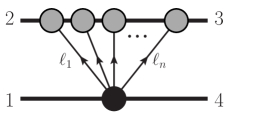
Figure 2: The generalized cut for leading order contributions to nonlinear tidal operators. Each blob is simply a (local) on-shell amplitude. The dark blob contains the $X^{n}$ tidal operator. The direction of graviton momentum flow is indicated by the arrows.

The amplitude with nonlinear tidal effect, i.e. the scattering with an $X^{n}$ operator insertion, where $X$ stands for $E$ or $B$, can be constructed from the unitarity cut in Fig. 2. We will mostly focus on leading contribution for such an operator in this section. In this case, the simplifications described in Section 3.1.1 are all applicable. Namely, the amplitude with $X^{n}$ tidal operator is still comprised of linearized electric and magnetic Weyl tensor in Eqs. (3.8) and (3.9); and the sewing of three-point amplitudes with the amplitude with $X^{n}$ tidal operator is effectively replacing the polarization $\varepsilon_{\mu\nu}(\ell_{i})\rightarrow T_{\mu\nu}(p_{2})$ for each graviton. Start from the the unitarity cut in Fig. 2. After sewing we find

$$\mathcal{M}_{{\rm X}^{n}}(\bm{p},\bm{q})= \frac{\kappa^{n}}{m_{2}^{n-1}}\int\mathcal{M}_{{\rm X}^{n}}(h(\ell_{1}),\dots,h(\ell_{n}),\phi(p_{1}),\phi(p_{4}))\big{|}_{\varepsilon_{\mu\nu}(\ell_{i})\rightarrow T_{\mu\nu}(p_{2})}$$

$$\quad\times\frac{1}{\ell_{1}^{2}\ell_{2}^{2}\cdots\ell_{n}^{2}}\left[\frac{i}{(-2u_{2}\cdot\ell_{1})}\frac{i}{(-2u_{2}\cdot\ell_{12})}\dotsc\frac{i}{(-2u_{2}\cdot\sum_{j=1}^{n-1}\ell_{j})}\right],$$ (4.1)

where we integrate over $\ell_{i}$ with $i=1,\dots,n-1$ and $\sum^{n}_{i=1}l_{i}=q$.

As discussed in the previous section, we can include spin degrees of freedom for the field without the tidal deformation by simply replacing in Eq (4.1) the point-particle stress tensor $T_{\mu\nu}$ with that of the general spinning particle $T^{\text{gen}}_{\mu\nu}$, cf. Eq. (3.17), or with that of a Kerr black hole, cf. (3.16).

The calculations from position space and momentum space also follow similarly as before. We discuss them in turn.

4.1 Leading order position-space analysis

Start with Eq. (4.1). Again we consider the rest frame of particle 2 in which we have Eq. (3.22). The first step is to integrate out energy in potential region. Using the identity [51]

$$\delta\left(\sum_{i=1}^{n}\ell^{0}_{i}\right)\left[\frac{i}{(-2u_{2}\cdot\ell_{1}+i0)}\frac{i}{(-2u_{2}\cdot\ell_{12}+i0)}\dotsc\frac{i}{(-2u_{2}\cdot\sum_{j=1}^{n-1}\ell_{j}+i0)}+\textrm{perm}\right]=\pi^{n-1}\prod_{i=1}^{n}\delta(\ell^{0}_{i})\,,$$ (4.2)

where perm is the rest of $n!$ permutations of $\ell_{1,\dots,n}$. Since the integrand is invariant under permutations, this localizes all $\ell^{0}_{i}=0$ with a $1/n!$ prefactor

$$\mathcal{M}_{{\rm X}^{n}}(\bm{p},\bm{q})= \frac{(-\kappa)^{n}}{(2m_{2})^{n-1}\,n!}\int\,\left[\prod_{i=1}^{n}\frac{d^{D-1}\bm{\ell}_{i}}{(2\pi)^{D-1}}\,\frac{1}{\bm{\ell}_{i}^{2}}\right]\,\delta\left(\bm{q}-\sum_{i=1}^{n}\bm{\ell}_{i}\right)$$

$$\quad\times\mathcal{M}_{{\rm X}^{n}}(h(\ell_{1}),\dots,h(\ell_{n}),\phi(p_{1}),\phi(p_{4}))\big{|}_{\varepsilon_{\mu\nu}(\ell_{i})\rightarrow T_{\mu\nu}(p_{2})},$$ (4.3)

To evaluate this integral, we use the same manipulations as at one loop. First consider the Fourier transform to position space

$$\mathcal{M}_{{\rm X}^{n}}(\bm{p},\bm{r})=\int\frac{d^{D-1}\bm{q}}{(2\pi)^{D-1}}e^{-i\bm{r}\cdot\bm{q}}\widetilde{\mathcal{M}}_{{\rm X}^{n}}(\bm{p},\bm{q})$$

$$\hskip 56.9055pt=\frac{(-\kappa)^{n}}{(2m_{2})^{n-1}\,n!}\prod_{i=1}^{n}\int\frac{d^{D-1}\bm{\ell}_{i}}{(2\pi)^{D-1}}\frac{e^{-i\bm{r}\cdot\bm{\ell}_{i}}}{\bm{\ell}_{i}^{2}}\,\mathcal{M}_{{\rm X}^{n}}(h(\ell_{1}),\dots,h(\ell_{n}),\phi(p_{1}),\phi(p_{4}))\big{|}_{\varepsilon_{\mu\nu}(\ell_{i})\rightarrow T_{\mu\nu}(p_{2})}$$

$$\hskip 56.9055pt=\frac{(-\kappa)^{n}}{(2m_{2})^{n-1}\,n!}\,\mathcal{M}_{{\rm X}^{n}}(h_{1},\dots,h_{n},\phi(p_{1}),\phi(p_{4})|\bm{r}),$$ (4.4)

where we use Eq. (3.3) to define

$$\,\mathcal{M}_{{\rm X}^{n}}(h_{1},\dots,h_{n},\phi(p_{1}),\phi(p_{4})|\bm{r})$$ (4.5)

$$\hskip 56.9055pt\equiv\prod_{i=1}^{n}\int\frac{d^{D-1}\bm{\ell}_{i}}{(2\pi)^{D-1}}\frac{e^{-i\bm{r}\cdot\bm{\ell}_{i}}}{\bm{\ell}_{i}^{2}}\,\mathcal{M}_{{\rm X}^{n}}(h(\ell_{1}),\dots,h(\ell_{n}),\phi(p_{1}),\phi(p_{4}))\big{|}_{\varepsilon_{\mu\nu}(\ell_{i})\rightarrow T_{\mu\nu}(p_{2})}$$

$$\hskip 56.9055pt=\,\mathcal{M}_{{\rm X}^{n}}(h(\ell_{1}),\dots,h(\ell_{n}),\phi(p_{1}),\phi(p_{4})|{X}_{\mu_{1}\mu_{2}}(\ell_{j},p_{1})\rightarrow{X}_{\mu_{1}\mu_{2}}(\bm{r}_{j},p_{1}),\bm{\ell}_{j}\rightarrow i\nabla_{j})\Big{|}_{\bm{r}_{j}\rightarrow\bm{r}}\,.$$

As before all the coordinates $\bm{r}_{j}$ are identified as $\bm{r}$ in the end. The above formula is very general and applies to higher multipole operators or general susceptibilities similar to Eq. (3.69). Recall that $\mathcal{M}_{{\rm X}^{n}}(h(\ell_{1}),\dots,h(\ell_{n}),\phi(p_{1}),\phi(p_{4}))$ is only a function of ${\cal E}_{\mu_{1}\mu_{2}}(\ell_{i},p_{2})$, ${\cal B}_{\mu_{1}\mu_{2}}(\ell_{i},p_{2})$, and Mandelstam invariants. The Fourier transform simply replaces them with their corresponding in position-space expressions defined in Eqs. (3.3) and (3.43). As before, the result of $\mathcal{M}_{{\rm X}^{n}}(\bm{p},\bm{r})$ is generally not isotropic, because any $u_{1}\cdot\ell$ in momentum space generates dependence on $\hat{\bm{z}}\cdot\bm{\ell}$. To bring it into the isotropic form, we Fourier transform back to momentum space, as in Eq. (3.39).

A simple example is the operator ${E}_{\mu}{}^{\nu}{E}_{\nu}{}^{\rho}{E}_{\rho}\,^{\mu}$, denoted as $(E^{3})$. With the contraction of three ${\cal E}$ tensors (3.3) given by

$${\cal E}_{\mu}{}^{\nu}(\bm{r},p_{1}){\cal E}_{\nu}{}^{\rho}(\bm{r},p_{1}){\cal E}_{\rho}\,^{\mu}(\bm{r},p_{1})=\frac{3m_{2}^{6}}{4096\pi^{3}|\bm{r}|^{13}}\,\left[9(\sigma^{2}-1)(\bm{r}^{2}-z^{2})(\sigma^{2}\bm{r}^{2}-(\sigma^{2}-1)z^{2})+2\bm{r}^{2}\right]\,,$$ (4.6)

the graviton-scalar amplitude is

$$\mathcal{M}_{({\rm E}^{3})}(h_{1},h_{2},h_{3},\phi(p_{1}),\phi(p_{4})|\bm{r})=12\kappa^{3}\,m_{1}\,{\cal E}_{\mu}{}^{\nu}(\bm{r},p_{1}){\cal E}_{\nu}{}^{\rho}(\bm{r},p_{1}){\cal E}_{\rho}\,^{\mu}(\bm{r},p_{1})\,.$$ (4.7)

Plugging into Eq. (4.4) then yields the four-scalar amplitude in position space

$$\mathcal{M}_{({\rm E}^{3})}(\bm{p},\bm{r})=-\frac{\kappa^{6}m_{1}}{2m_{2}^{2}}\,{\cal E}_{\mu}{}^{\nu}(\bm{r},p_{1}){\cal E}_{\nu}{}^{\rho}(\bm{r},p_{1}){\cal E}_{\rho}{}^{\mu}(\bm{r},p_{1}).$$ (4.8)

Using the Fourier transform formula in Eq. (3.40), we arrive the final result

$${\mathcal{M}}_{({\rm E}^{3})}(\bm{p},\bm{q}) =\frac{-|\bm{q}|^{6-4\epsilon}}{2\epsilon}\,\overline{{\mathcal{M}}}_{({\rm E}^{3})}(\bm{p})=\frac{18}{11!!}G^{3}m_{1}m_{2}^{4}\pi{}\Bigl{(}\frac{7}{4}-9\sigma^{2}+10\sigma^{4}\Bigr{)}\frac{|\bm{q}|^{6-4\epsilon}}{\epsilon}\,.$$ (4.9)

An important feature of the position-space scalar-graviton amplitude (4.5), which we already encountered in the one-loop analysis in Sec. 3.3, is that it factorizes into a product of position-space ${\cal E}$ tensor, defined in Eq. (3.3) and its magnetic counterpart, perhaps with additional derivatives. As explained in Sec. 2, the fact that these position-space tensors have rank 3 implies that such a product can be further expressed as a sum of products of traces of at most three factors. For example, Eq. (2.53) gives the decomposition of any power of a rank-3 matrix in terms of in terms of traces of two and three such matrices. It applies directly to the four-scalar amplitude with an insertion of $(E^{n})$ and expresses it as a sum of four-scalar amplitudes with an insertion of $(E^{2})^{n_{2}}(E^{3})^{n_{3}}$ with $n=2n_{2}+3n_{3}$. It also applies directly to amplitudes with an insertion of $(B^{n})$. While the resulting amplitude vanishes of $n$ is odd, it also further simplifies if $n$ is even. The parity-odd nature of ${\cal B}_{\mu,\nu}(\bm{r},\bm{p})$ and position-space factorization imply that, to leading order, $(B^{3})$ = 0 because there are insufficient vectors to saturate the Levi-Civita tensor. Therefore, to leading order, the analog of Eq. (2.53) for the magnetic operators reduces to

$$(B^{n=2k})=\frac{1}{2^{k-1}}(B^{2})^{k}\,.$$ (4.10)

The amplitudes collected in the Appendix A verify these formulas for up to $n=8$.

The momentum-space four-scalar amplitude is related to the position-space four-scalar amplitude by single $(D-1)$-dimensional Fourier transform. The structure of the position-space amplitude is essential. This observation allows us to evaluate amplitudes and the corresponding two-body potentials to leading order for arbitrary operators.

Since the position-space scalar-graviton amplitudes with one insertion of either one of $(E^{2})$, $(B^{2})$ or $(E^{3})$ have a similar structure, we will discuss them simultaneously, referring to these operators as $(\mathcal{O})$. They have the form,

$${\widetilde{\mathcal{M}}}_{(\mathcal{O})}={\mathcal{N}}_{(\mathcal{O})}\frac{1}{\bm{r}^{h}}\Bigl{(}a_{(\mathcal{O})}+b_{(\mathcal{O})}\frac{(\bm{r}\cdot\bm{u}_{1})^{2}}{\bm{r}^{2}}+c_{(\mathcal{O})}\frac{(\bm{r}\cdot\bm{u}_{1})^{4}}{\bm{r}^{4}}\Bigr{)}\,,$$ (4.11)

where $\mathcal{N}_{(\mathcal{O})}$ is an operator-dependent normalization factor. For the three operators it is,

$${\mathcal{N}}_{(\rm E^{2})}={\mathcal{N}}_{(\rm B^{2})}=2^{4}G^{2}\pi^{2}m_{1}m_{2}^{3}\,,\hskip 56.9055pt{\mathcal{N}}_{(\rm E^{3})}=2^{5}G^{3}\pi^{3}m_{1}m_{2}^{4}\,,$$ (4.12)

and the coefficients are

$$a_{\rm(E^{2})} =\frac{3(1-3\sigma^{2}+3\sigma^{4})}{2\pi^{2}}\,,\hskip 51.21504ptb_{\rm(E^{2})}=\frac{9(1-2\sigma^{2})}{2\pi^{2}}\,,\hskip 59.75095ptc_{\rm(E^{2})}=\frac{9}{2\pi^{2}}\,,$$

$$a_{\rm(B^{2})} =\frac{9\sigma^{2}(\sigma^{2}-1)}{2\pi^{2}}\,,\hskip 76.82234ptb_{\rm(B^{2})}=\frac{9(1-2\sigma^{2})}{2\pi^{2}}\,,\hskip 59.75095ptc_{\rm(B^{2})}=\frac{9}{2\pi^{2}}\,,$$

$$a_{\rm(E^{3})} =-\frac{3(2-9\sigma^{2}+9\sigma^{4})}{8\pi^{3}}\,,\hskip 42.67912ptb_{\rm(E^{3})}=-\frac{27(1-2\sigma^{2})}{8\pi^{3}}\,,\hskip 42.67912ptc_{\rm(E^{3})}=-\frac{27}{8\pi^{3}}\,.$$ (4.13)

The exponent of the overall $\bm{r}$ factor is $h=6$ for $({\cal O})=(E^{2})$ and $({\cal O})=(B^{2})$ and $h=9$ for $({\cal O})=(E^{3})$.

The position- space amplitude with an insertion of an operator made up of $n$ such traces is simply given by raising (4.11) to the $n$th power and adjusting the normalization factor,

$${\widetilde{\mathcal{M}}}_{(\mathcal{O})^{n}}={\mathcal{N}}_{(\mathcal{O})^{n}}\Bigl{[}\frac{1}{\bm{r}^{h}}\biggl{(}a_{(\mathcal{O})}+b_{(\mathcal{O})}\frac{(\bm{r}\cdot\bm{u}_{1})^{2}}{\bm{r}^{2}}+c_{(\mathcal{O})}\frac{(\bm{r}\cdot\bm{u}_{1})^{4}}{\bm{r}^{4}}\Bigr{)}\biggr{]}^{n}\,.$$ (4.14)

The change in normalization factor is related to the normalization of the tree-level amplitude with one insertion of the composite operator. We find

$${\mathcal{N}}_{(\rm E^{2})^{n}}={\mathcal{N}}_{(\rm B^{2})^{n}}=2^{2n+2}G^{2n}\pi^{2n}m_{1}m_{2}^{2n+1}\,,\qquad{\mathcal{N}}_{(\rm E^{3})^{n}}=2^{3n+2}G^{3n}\pi^{3n}m_{1}m_{2}^{3n+1}\,.$$ (4.15)

To obtained the momentum-space scattering amplitude with an insertion of an arbitrary operator $({\cal O})^{n}$ we first use twice the binomial expansion and put the position-space amplitude in the form

$${\widetilde{\mathcal{M}}}_{(\mathcal{O})^{n}}=\frac{{\mathcal{N}}_{(\mathcal{O})^{n}}}{\bm{r}^{nh}}\sum_{k=0}^{n}\sum_{l=0}^{k}{{n}\choose{k}}{{k}\choose{l}}a_{\mathcal{O}}^{n-k}\,b_{\mathcal{O}}^{l}\,c_{\mathcal{O}}^{k-l}\,\biggl{(}\frac{(\bm{r}\cdot\bm{u}_{1})^{2}}{\bm{r}^{2}}\biggr{)}^{\!2k-l}\,.$$ (4.16)

Using then the general tensor Fourier-transform relation (3.40) which enforces $\bm{q}\cdot\bm{u}_{1}=\bm{q}^{2}/2\rightarrow 0$ leads to the desired result:

$${\cal M}_{(\mathcal{O})^{n}}(\bm{p},\bm{q}) =\frac{{\mathcal{N}}_{(\mathcal{O})^{n}}}{|\bm{q}|^{D-nh-1}}\sum_{k=0}^{n}\sum_{l=0}^{k}{{n}\choose{k}}{{k}\choose{l}}a_{\mathcal{O}}^{n-k}\,b_{\mathcal{O}}^{l}\,c_{\mathcal{O}}^{k-l}$$ (4.17)

$$\qquad\times\frac{2^{D-hn-1}\pi^{D/2}(\sigma^{2}-1)^{2k-l}\Gamma(\frac{1}{2}+2k-l)}{\sin(\frac{\pi}{2}(D-hn-1))\Gamma(\frac{1}{2}(3+hn-D))\Gamma(2k-l+\frac{1}{2}hn)}\,,$$

where $D=4-2\epsilon$. The two-body potential and the eikonal phase follow then straightforwardly via Eqs. (2.9)-(2.12):

$$\hskip-8.5359ptV_{(\mathcal{O})^{n}}(\bm{p},\bm{r}) =-\frac{{\mathcal{N}}_{(\mathcal{O})^{n}}}{4E_{1}E_{2}\;|\bm{r}|^{nh}}\sum_{k=0}^{n}\sum_{l=0}^{k}{{n}\choose{k}}{{k}\choose{l}}a_{\mathcal{O}}^{n-k}\,b_{\mathcal{O}}^{l}\,c_{\mathcal{O}}^{k-l}\,(\sigma^{2}-1)^{2k-l}\frac{\Gamma(\frac{1}{2}+2k-l)\Gamma(\frac{1}{2}hn)}{\sqrt{\pi}\Gamma(2k-l+\frac{1}{2}hn)}\,,$$ (4.18)

$$\hskip-8.5359pt\delta_{(\mathcal{O})^{n}}(\bm{p},\bm{b}) =\frac{{\mathcal{N}}_{(\mathcal{O})^{n}}}{4m_{1}m_{2}\;|\bm{b}|^{nh-1}}\sum_{k=0}^{n}\sum_{l=0}^{k}{{n}\choose{k}}{{k}\choose{l}}a_{\mathcal{O}}^{n-k}\,b_{\mathcal{O}}^{l}\,c_{\mathcal{O}}^{k-l}\,(\sigma^{2}-1)^{2k-l-1/2}\frac{\Gamma(\frac{1}{2}+2k-l)\Gamma(\frac{1}{2}(hn-1))}{\Gamma(2k-l+\frac{1}{2}hn)}\,.$$

As discussed earlier, parity and factorization of the position-space amplitude implies that, to leading order in the classical limit, amplitudes with an insertion of an operator which has at least one parity-odd factor vanish identically even if the operator is overall parity-even. Thus, Eq. (2.53) with $E\rightarrow B$ implies that the approach described here yields the two-body potential for all nonlinear tidal operators of the type $(B^{2n})$.

The discussion above can be easily extended to cover amplitudes with one insertion of $(E^{n})$. Eq. (2.53) expresses it as a linear combination of amplitudes with one insertion of $(E^{2})^{n_{2}}(E^{3})^{n_{3}}$ with $2n_{2}+3n_{3}=n$. The position space form of the latter involves a product of two factors analogous to the right-hand side of Eq. (4.14). Each of them can be binomially expanded (with a slight simplification based on the equality $b_{(E^{2})}/b_{(E^{3})}=c_{(E^{2})}/c_{(E^{3})}$ visible in Eq. (4.13)) and put in a form analogous to the right-hand side of Eq. (4.16). Fourier-transforming using Eq. (3.40) and putting together all terms leads to the momentum-space amplitude with one insertion of $(E^{n})$.

The general formulas above show explicitly that the difference $E^{2n}-B^{2n}$ is subleading in the high-energy limit. This extends the observations of Refs. [28, 29] beyond the linear order.

4.2 Order by order momentum-space analysis

The above position-space evaluation is a very effective means for evaluating leading contributions to any given tidal operator. Momentum-space methods for evaluating the loop integrals instead offer a straightforward way to systematically extend the results to higher orders following the methods presented in Refs. [11, 12, 13]. Indeed following these methods, next to leading order contributions to $E^{2}$ and $B^{2}$ tidal operators were evaluated in Ref. [21]. A related approach for tidal operators based on world lines has been recently given in Ref. [29] where additional $E^{2}$ operators were evaluated.

Here we first re-evaluate the amplitudes in momentum space through $C^{4}$ and then discuss the extension to higher orders. The starting point is again the generalized cut shown in Fig. 2. We evaluate the expressions in $D$-dimensions. Here we do not make use of the special real-space factorization of the integrals discussed in the previous section, but rather simply carry out the evaluation of the cut and then reduce the result to a basis of independent momentum products. We can simplify the resulting expressions considerably by applying the cut conditions and expanding in small momentum transfer $q$. Specifically, we can choose a basis of momentum invariants which does not contain any of the products ($p_{2}\cdot\ell_{k}$), since the cut conditions give

$$\left(-p_{2}+\sum_{i=1}^{k}\ell_{i}\right)^{2}-m_{2}^{2}=0\, \rightarrow\,\,(p_{2}\cdot\ell_{k})=\sum_{i=2}^{k}\sum_{j=1}^{i-1}(\ell_{i}\cdot\ell_{j})-\sum_{i=1}^{k-1}(p_{2}\cdot\ell_{i})\,,$$ (4.19)

where the final term can be eliminated inductively starting with $p_{2}\cdot\ell_{1}=0$. Products of the form ($p_{3}\cdot\ell_{k}$) can then be eliminated using momentum conservation $p_{3}=-p_{2}-q=-p_{2}-\sum\ell_{i}$. Since the cut graviton momenta scale as ${\mathcal{O}}(q)$, the cut conditions thus ensure that the scaling of ($p_{2}\cdot\ell_{k}$) or ($p_{3}\cdot\ell_{k}$), which naively would be ${\mathcal{O}}(q)$, instead scale as ${\mathcal{O}}(q^{2})$. This greatly aids in the simplification of the integrand after expanding in small $q$.

Unlike in the position-space analysis, the integrals do not decouple into a product, and in general, the momentum-space integrals can be challenging to evaluate. To do so, we use FIRE6 [52] which uses integration by parts methods [35] to reduce the integrals a single master integral, which can then be evaluated either by direct integration or by differential equations [53]. Evaluating the integrals is the most significant bottleneck for this method, but the task is significantly aided by the use of special variables as described in [36],

$$p_{1}=-(\bar{p}_{1}-q/2)\,,\hskip 22.76228ptp_{4}=\bar{p}_{1}+q/2\,,\hskip 22.76228ptp_{2}=-(\bar{p}_{2}+q/2)\,,\hskip 22.76228ptp_{3}=\bar{p}_{2}-q/2\,.$$ (4.20)

The $\bar{p}_{i}$ are orthogonal to $q$ by construction: $\bar{p}_{i}\cdot q=0$. As described in more detail in Ref. [36], with these variables the matter propagators reduce to

$$\frac{1}{\left(p_{2}+\ell_{1\cdots i}\right)^{2}-m_{2}^{2}}=\frac{1}{2\bar{p}_{2}\cdot\ell_{1\cdots i}}+{\mathcal{O}}(q^{0})\,,$$ (4.21)

so the matter propagators are linear in the loop momenta. In addition, we can define normalized external momenta, $\bar{u}_{i}^{\mu}={\bar{p}_{i}^{\mu}}/{\sqrt{m_{i}^{2}-{q^{2}}/4}}$, such that $\bar{u}_{i}^{2}=1$ The net effect is that the $q^{2}$ dependence is scaled out of the integral so that it is only a function of a single-scale $\bar{u}_{1}\cdot\bar{u}_{2}=\sigma+\mathcal{O}(q^{2})$. Using these variables integral encountered at any order of perturbation theory can then be converted to a single scale integral. Such integrals are quite amenable to integration-by-parts methods, greatly speeding the evaluation.

The restriction to the potential region precludes pinching any propagators and the existence of irreducible scalar products. Thus, the result of IBP reduction is a single master integral, with a coefficient given by powers of $\bm{q}$ dictated by dimensional analysis, as well as a polynomial in $\sigma$. The master integral is the scalar fan integral in Fig. 3, which can be easily evaluated by factorizing the loops by going to position space and Fourier transforming back, with the result

$$I_{\text{fan}}^{(L)} =\int\left(\prod_{i=1}^{L+1}\frac{d^{D}\ell}{(2\pi)^{D}}\frac{1}{\ell_{i}^{2}}\right)\frac{|\bm{q}|^{2-L}\delta(\sum_{i}\ell_{i}-q)}{(-2u_{2}\cdot\ell_{1}+i0)(-2u_{2}\cdot\ell_{12}+i0)\cdots(-2u_{2}\cdot\ell_{1\cdots n-1}+i0)}$$

$$=\frac{i^{L+2}}{2^{L(4-2\epsilon)}\pi^{L\left(\frac{3}{2}-\epsilon\right)}}\frac{\Gamma\left(\frac{1}{2}-\epsilon\right)^{L+1}\Gamma\left((\epsilon-\frac{1}{2})L+1\right)}{\Gamma(L+2)\Gamma\left((\frac{1}{2}-\epsilon)(L+1)\right)}|\bm{q}|^{-2\epsilon L}\,.$$ (4.22)

At one loop this agrees with Eq. (3.25) with $l=0$, and at two and three loops it yields

$$I_{\text{fan}}^{(2)}=\frac{1}{768\pi^{2}}\frac{(\bm{q}^{2})^{-2\epsilon}}{2\epsilon}+\mathcal{O}(\epsilon^{0})\,,\hskip 42.67912ptI_{\text{fan}}^{(3)}=-\frac{i}{49152\pi^{2}}+\mathcal{O}(\epsilon)\,.$$ (4.23)

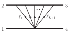
Figure 3: The $L$-loop fan integral.

The results of the IBP reduction at two loops gives the amplitudes with a single insertion of the tidal operators in terms of a single master integral:

$${\mathcal{M}}_{\rm(E^{3})} =\frac{1024}{385}\pi^{3}G^{3}m_{1}m_{2}^{4}|\bm{q}|^{6}\left(\frac{7}{4}-9\sigma^{2}+10\sigma^{4}\right)I_{\text{fan}}^{(2)}\,,$$

$${\mathcal{M}}_{\rm(EB^{2})} =\frac{1024}{1155}\pi^{3}G^{3}m_{1}m_{2}^{4}|\bm{q}|^{6}\left(\sigma^{2}-1\right)\left(1+10\sigma^{2}\right)I_{\text{fan}}^{(2)}\,,$$

$${\mathcal{M}}_{\rm(B^{3})} ={\mathcal{M}}_{\rm E^{2}B}=0\,.$$ (4.24)

As expected, the parity odd operators $E^{2}B$ and $B^{3}$ operator do not contribute.

At three loops, by reducing the integrand to the sole master integral we find the following for the amplitudes with an insertion of the single trace operators,

$$\mathcal{M}_{\rm(E^{4})} =-i\frac{983}{9031680}\pi^{4}G^{4}m_{1}m_{2}^{5}|\bm{q}|^{9}(1231-7304\sigma^{2}+18590\sigma^{4}-22880\sigma^{6}+12155\sigma^{8})I^{(3)}_{\text{fan}}\,,$$

$$\mathcal{M}_{\rm(B^{4})} =-i\frac{140569}{9031680}\pi^{4}G^{4}m_{1}m_{2}^{5}|\bm{q}|^{9}(\sigma^{2}-1)^{2}(1+10\sigma^{2}+85\sigma^{4})I^{(3)}_{\text{fan}}\,,$$

$$\mathcal{M}_{\rm(EEBB)} =-i\frac{10813}{27095040}\pi^{4}G^{4}m_{1}m_{2}^{5}|\bm{q}|^{9}(\sigma^{2}-1)(41+689\sigma^{2}-2925\sigma^{4}+3315\sigma^{6})I^{(3)}_{\text{fan}}\,,$$

$$\mathcal{M}_{\rm(EBEB)} =i\frac{10813}{27095040}\pi^{4}G^{4}m_{1}m_{2}^{5}|\bm{q}|^{9}(\sigma^{2}-1)(25+481\sigma^{2}-2925\sigma^{4}+3315\sigma^{6})I^{(3)}_{\text{fan}}\,.$$ (4.25)

Similarly, the amplitudes with double trace insertions evaluate to,

$$\mathcal{M}_{\rm(E^{2})^{2}} =-i\frac{983}{4515840}\pi^{4}G^{4}m_{1}m_{2}^{5}|\bm{q}|^{9}(1231-7304\sigma^{2}+18590\sigma^{4}-22880\sigma^{6}+12155\sigma^{8})I^{(3)}_{\text{fan}}\,,$$

$$\mathcal{M}_{\rm(B^{2})^{2}} =-i\frac{140569}{4515840}\pi^{4}G^{4}m_{1}m_{2}^{5}|\bm{q}|^{9}(\sigma^{2}-1)^{2}(1+10\sigma^{2}+85\sigma^{4})I^{(3)}_{\text{fan}}\,,$$

$$\mathcal{M}_{\rm(E^{2})(B^{2})} =-i\frac{10813}{4515840}\pi^{4}G^{4}m_{1}m_{2}^{5}|\bm{q}|^{9}(\sigma^{2}-1)(19+299\sigma^{2}-975\sigma^{4}+1105\sigma^{6})I^{(3)}_{\text{fan}}\,,$$

$$\mathcal{M}_{\rm(EB)^{2}} =0\,,$$ (4.26)

It is not difficult to check that these results satisfy the four-dimensional relations described in Sec. 2. In addition, they agree with the results obtained in the previous section for tidal operators with arbitrary numbers of $E$s and $B$s and collected in the Appendix for a variety of operators up to $E^{8}$ and $B^{8}$.

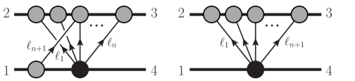
Figure 4: The generalized cuts that need to be evaluated at next to leading order for an $R^{n}$ type tidal operator.

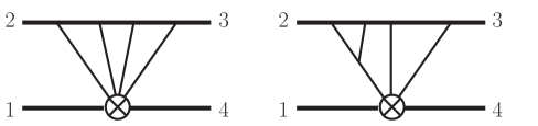
Figure 5: Sample diagrams for next-to-leading-order contributions for the $R^{3}$ tidal operators which are simple to evaluate.

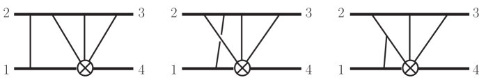
Figure 6: Sample diagrams next-to-leading order contributions for the $R^{3}$ tidal operators that involve iteration contributions or nontrivial integrals.

An important aspect of the momentum-space approach is that it gives a systematic means for obtaining corrections higher order in Newton’s constant for any operator insertion. For example Fig. 4 shows the generalized cuts that would need to be evaluated to obtain the next-to-leading order corrections from an $C^{3}$ tidal operator. In the first of these cuts the four-point amplitude can appear at any location on the top matter line. The mapping of the integrands resulting from these cuts onto a integral basis generates a number of diagrams. For example, in Fig. 5 we show a sample of the diagrams that that are quite easy to evaluate for an $R^{3}$ tidal operator, as we can again evaluate the integral using the real-space technique presented in the previous section. More complicated diagrams that involve iteration contributions or non-trivial integrations are shown in Fig. 6. In these cases, the integrals do not factorize, but the momentum-space approach of evaluating cuts and reducing to a basis of master integrals will still be quite feasible. As noted in Refs. [15, 21] the probe limit simplifies the evaluation of the contributions. In any case, it is clear that amplitude methods can be applied beyond leading order to understand the systematics of higher-dimension operators. We leave this to future studies.

5 Effective field theory extensions of GR

The same methods apply just as well to any operator, not just the tidal ones. For example, we can consider the $R^{n}$ operators arising from unknown short distance physics. Here we will not classify such operators, but pick illustrative examples. The effect of operators up to $R^{4}$ has already been discussed in some detail in Refs. [38, 39, 40]. In order to be concrete here we discuss an effective action of the form

$$S=\frac{1}{16\pi G}\int d^{D}x\sqrt{-g}\left(-R+c_{K}K_{\mu_{1}...\rho_{n}}R^{\mu_{1}\nu_{1}\sigma_{1}\rho_{1}}R^{\mu_{2}\nu_{2}\sigma_{2}\rho_{2}}\cdots R^{\mu_{n}\nu_{n}\sigma_{n}\rho_{n}}\right)\,,$$ (5.1)

where the first term is the usual Einstein-Hilbert action, and $K_{\mu_{1}...\rho_{n}}$ merely gives the contraction between the Riemann tensors. Each independent contraction carries an independent Wilson coefficient $c_{K}$.

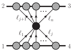
Figure 7: Cut for a general $R^{n}$ type operator. In the case $j=1$, it is convenient to take the single graviton attaching to the bottom matter line as off shell and part of a tree amplitude including the lower massive scalar line. All other gravitons and exposed matter lines are taken on shell. The direction of graviton momentum flow is indicated by the arrows.

We construct the integrands for pure $R^{n}$ modifications of gravity in a similar manner as for those of the tidal operators. The leading contribution to the potential due to $R^{n}$ operators is captured by the cuts in Fig. 7. The diagrams in general are a product of two fan diagrams, where all graviton legs, as well as the matter lines between the three point vertices, are on shell, the exception being the case where $(n-1)$ on-shell gravitons attach to one of the matter lines, while one graviton which we take to be off shell attaches to the other matter line. In this case, it is convenient to include the matter line to which the single graviton propagator is attached as part of a single tree amplitude.

To evaluate the cuts in Fig. 7 we use the replacement derived above (see Eq. (3.11)). This simplifies the form of the Riemann tensor:

$$R^{\mu\nu\rho\sigma}(\ell_{i})\big{|}_{\varepsilon_{\mu\nu}(\ell_{i})\rightarrow T_{\mu\nu}(p_{a})}=-\frac{1}{2}\left(\ell_{i}^{\mu}\ell_{i}^{\rho}\left(p_{a}^{\nu}p_{a}^{\sigma}-\frac{1}{2}\eta^{\nu\sigma}m_{a}^{2}\right)-(\sigma\leftrightarrow\rho)\right)+((\mu,\rho)\leftrightarrow(\nu,\sigma))+\mathcal{O}(q^{3})\,,$$ (5.2)

where $p_{a}$ and $m_{a}$ are the momentum and mass of the matter line the graviton attaches to. When contracted in sequence with other gravitons attaching to the same matter line, products involving the matter momenta in the above expression must reduce to $p_{a}\cdot p_{a}=m_{a}^{2}$, or the $q$ scaling will become sub-leading, as shown in the previous section.

The cut corresponding to Fig. 7 is simply a product of two fans,

$${\mathcal{C}}_{R^{n}}=K_{\mu_{1}...\rho_{n}}{\mathcal{O}}^{\mu_{1}...\rho_{j}}(\ell_{1},...,\ell_{j};p_{1}){\mathcal{O}}^{\mu_{j+1}...\rho_{n}}(\ell_{j+1},...,\ell_{n};p_{2})\,,$$ (5.3)

where, for instance,

$${\mathcal{O}}^{\mu_{1}...\rho_{j}}(\ell_{1},...,\ell_{j};p_{1})=R_{1}^{\mu_{1}\nu_{1}\sigma_{1}\rho_{1}}\cdots R_{j}^{\mu_{j}\nu_{j}\sigma_{j}\rho_{j}}\big{|}_{\varepsilon_{\mu\nu}(\ell_{i})\rightarrow T_{\mu\nu}(p_{1})}\,.$$ (5.4)

As in previous sections, the integrands obtained after restoring the cut propagators are also well suited for applying position-space techniques. In this case, we must introduce a fictitious momentum transfer $\bm{q}^{\prime}$ such that the integrand decouples in two parts, corresponding to the two terms in Eq. (5.3) decouple, and the corresponding propagators attached to one matter line or the other. The energy integrations can be carried out as in the previous sections with the result

$$\mathcal{M}_{R^{n}}(\bm{p},\bm{q}) =K_{\mu_{1}...\rho_{n}}\int d^{D-1}\bm{q}^{\prime}\,\delta(\bm{q}+\bm{q}^{\prime})\int\left(\prod_{a=1}^{j}\frac{d^{D-1}\bm{\ell}_{a}}{(2\pi)^{D-1}}\right)\frac{\delta(\sum_{a=1}^{j}\bm{\ell}_{a}+\bm{q}^{\prime}){\mathcal{O}}^{\mu_{1}...\rho_{j}}(\bm{\ell}_{1},...,\bm{\ell}_{j};p_{1})}{\bm{\ell}_{1}^{2}\cdots\bm{\ell}_{j}^{2}}$$

$$\hskip 56.9055pt\times\int\left(\prod_{a=j+1}^{n}\frac{d^{D-1}\bm{\ell}_{a}}{(2\pi)^{D-1}}\right)\frac{\delta(\sum_{a=j+1}^{n}\bm{\ell}_{a}-\bm{q}){\mathcal{O}}^{\mu_{j+1}...\rho_{n}}(\bm{\ell}_{j+1},...,\bm{\ell}_{n};p_{2})}{\bm{\ell}_{j+1}^{2}\cdots\bm{\ell}_{n}^{2}}\,.$$ (5.5)

Writing

$$\delta(\bm{q}+\bm{q}^{\prime})=\int\frac{d^{D-1}\bm{x}}{(2\pi)^{D-1}}e^{i(\bm{q}+\bm{q}^{\prime})\cdot\bm{x}}$$ (5.6)

and taking the Fourier transform of the amplitude we find

$$\mathcal{M}_{R^{n}}(\bm{p},\bm{r}) =\int\frac{d^{D-1}\bm{q}}{(2\pi)^{D-1}}e^{-i\bm{q}\cdot\bm{r}}\mathcal{M}_{R^{n}}(\bm{p},\bm{q})$$

$$=K_{\mu_{1}...\rho_{n}}\int d^{D-1}\bm{x}\int\left(\prod_{a=1}^{j}\frac{d^{D-1}\bm{\ell}_{a}}{(2\pi)^{D-1}}\frac{e^{-i\bm{\ell}_{a}\cdot\bm{x}}}{\bm{\ell}_{a}^{2}}\right){\mathcal{O}}^{\mu_{1}...\rho_{j}}(\bm{\ell}_{1},...,\bm{\ell}_{j};p_{1})$$

$$\hskip 28.45274pt\times\int\left(\prod_{a=j+1}^{n}\frac{d^{D-1}\bm{\ell}_{a}}{(2\pi)^{D-1}}\frac{e^{-i\bm{\ell}_{a}\cdot(\bm{r}-\bm{x})}}{\bm{\ell}_{a}^{2}}\right){\mathcal{O}}^{\mu_{j+1}...\rho_{n}}(\bm{\ell}_{j+1},...,\bm{\ell}_{n};p_{2})$$

$$=K_{\mu_{1}...\rho_{n}}\int d^{D-1}\bm{x}\,{\mathcal{O}}^{\mu_{1}...\rho_{j}}(\bm{x};p_{1}){\mathcal{O}}^{\mu_{j+1}...\rho_{n}}(\bm{r}-\bm{x};p_{2})\,.$$ (5.7)

The product in momentum space has become a convolution in position space over $\bm{x}$, which can be viewed as the position in the bulk, i.e. away from the massive particle trajectories, at which the $R^{n}$ operator is inserted. Note however that this formula does not have a natural interpretation in position space, given that the energy integrals in each factor were performed by going to the rest frame of different particles. In practice, as in previous sections, this formula can be used by transforming one last time to momentum space, so that the convolution is trivialized and each factor can be written in isotropic coordinates.

The inclusion of derivatives, $\nabla^{2m}R^{n}$, or of spin on the matter lines poses no obstruction to applying this method. In the former case one must organize the additional powers of loop momentum in the integrand into either factor in analogy with Eq. (5.3). The factorization argument carries over and the additional loop momenta become derivatives in position space acting on either factor of Eq. (5.7). For the case of spin, the only difference is that the Fourier transforms in Eq. (5.7) become non-Abelian Fourier transforms defined in Eq. (3.92).

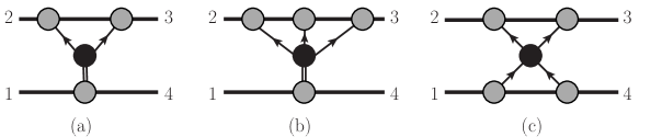
Figure 8: The corrections from (a) $R^{3}$ and (b,c) $R^{4}$ operators that appear in EFT extensions of GR. The double-line notation indicates that we have not used on-shell conditions on that line.

As simple examples, consider the cases of ${\mathcal{O}}_{R^{3}}=R^{\mu_{1}\nu_{1}}{}_{\mu_{2}\nu_{2}}R^{\mu_{2}\nu_{2}}{}_{\mu_{3}\nu_{3}}R^{\mu_{3}\nu_{3}}{}_{\mu_{1}\nu_{1}}$ and ${\mathcal{O}}_{(R^{2})^{2}}=(R^{\mu_{1}\nu_{1}}{}_{\mu_{2}\nu_{2}}R^{\mu_{2}\nu_{2}}{}_{\mu_{1}\nu_{1}})^{2}$. The contributing generalized unitarity cut for the $R^{3}$ operator are shown in Fig. 8(a) while the two potentially contributing cuts for the the $R^{4}$ operator are shown in Fig. 8(b,c). In the diagrams the double-line notation indicates that we have not used on-shell conditions on that line, but consider the two connected blobs as part of a single tree amplitude.

After carrying out the integration, the $R^{3}$ and $R^{4}$ amplitudes are

$${\mathcal{M}}_{R^{3}}= -6c_{R^{3}}G^{2}\pi^{2}m_{1}^{2}m_{2}^{2}(m_{1}+m_{2})|\bm{q}|^{3}(\sigma^{2}-1)\,,$$

$${\mathcal{M}}_{(R^{2})^{2}}= -\frac{2^{7}}{315}c_{(R^{2})^{2}}G^{3}\pi m_{1}^{2}m_{2}^{2}(m_{1}^{2}+m_{2}^{2})\frac{({\bm{q}}^{2})^{3-2\epsilon}}{2\epsilon}(3\sigma^{2}-1)\,,$$ (5.8)

where we took the operators to have coefficient $c_{R}^{3}$ and $c_{(}R^{2})^{2}$ respectively. Taking the Fourier transform (2.12) to position space gives the potentials

$$V_{R^{3}} =\frac{18}{E_{1}E_{2}}c_{R^{3}}G^{2}m_{1}^{2}m_{2}^{2}(m_{1}+m_{2})(\sigma^{2}-1)\,\frac{1}{r^{6}}\,,$$

$$V_{(R^{2})^{2}} =\frac{2^{8}}{E_{1}E_{2}}c_{(R^{2})^{2}}G^{3}\,m_{1}^{2}m_{2}^{2}(m_{1}^{2}+m_{2}^{2})(3\sigma^{2}-1)\,\frac{1}{r^{9}}\,.$$ (5.9)

The ${\mathcal{O}}_{R^{3}}$ amplitude and potential was obtained previously in Refs. [39, 40] and we find agreement. In Ref. [39] the authors also evaluate the effect of an additional $R^{3}$ operator,

$$G_{3}={\mathcal{O}}_{R^{3}}-R^{\mu\nu\alpha}{}_{\beta}R^{\beta\gamma}{}_{\nu\sigma}R^{\sigma}{}_{\mu\gamma\alpha}\,;$$ (5.10)

this is related to tidal operators via a field redefinition up to operators that vanish in four dimensions. This can be seen by evaluating its four-dimensional four-point amplitude, which feeds into the two-graviton cut, using spinor-helicity methods [39]:

$${\mathcal{M}}_{G^{3}}(\phi(p_{1}),h^{++}(k_{2}),h^{++}(k_{3}),\phi(p_{4}))\propto[23]^{4}(-q^{2}+2m_{1}^{2})\,.$$ (5.11)

Since this is a local contribution, it is already captured by tidal operators of the form $E^{2}$, $B^{2}$. Interestingly, though, if this operator were present with a sufficiently large coefficient, it would produce a result equivalent to the leading tidal Love numbers, even if these are set identically to zero for black holes in Einstein gravity [32].

The leading PN contribution from the $R^{4}$ operator (${\mathcal{O}}_{(R^{2})^{2}}$) was calculated in Ref. [38], with which we find agreement. We can also easily determine that the other operators considered in Ref. [38] give no contribution to the leading conservative potential. The contribution from ${\mathcal{O}}_{(R^{2})(R\tilde{R})}=(R^{\mu_{1}\nu_{1}}{}_{\alpha\beta}\epsilon^{\alpha\beta}{}_{\mu_{2}\nu_{2}}R^{\mu_{2}\nu_{2}}{}_{\mu_{1}\nu_{1}})(R^{\mu_{3}\nu_{3}}{}_{\mu_{4}\nu_{4}}R^{\mu_{4}\nu_{4}}{}_{\mu_{3}\nu_{3}})$ is zero simply because it is parity-odd. The operator ${\mathcal{O}}_{(R\tilde{R})^{2}}=(R^{\mu_{1}\nu_{1}}{}_{\alpha\beta}\epsilon^{\alpha\beta}{}_{\mu_{2}\nu_{2}}R^{\mu_{2}\nu_{2}}{}_{\mu_{1}\nu_{1}})^{2}$, while being parity even, contributes zero at leading order, in analogy to the tidal operator ${\mathcal{O}}_{(EB)^{2}}$. In both cases, the factorization of the integrand in real space forces the separate parity-odd factors to evaluate to zero, as discussed in Section 4.1

Here we refrain from evaluating the amplitudes for the $R^{5}$ and higher operators. However, in these cases, there is an additional link between the $R^{n}$ extensions of Einstein gravity and the tidal operators. After carrying out the soft expansion of the integrand for the $R^{n}$ operators, one encounters ultraviolet divergences that renormalize tidal operators [5]. For example, in principle the $R^{5}$ operator, which produces a diagram with three gravitons attached to one matter line and two attached to the other, could produce a UV subdivergence and thereby renormalize $E^{2}$ or $B^{2}$ tidal operators (with additional derivatives). It would be an interesting problem to systematically study this interplay for infinite sequences of $R^{n}$ operators.

6 Conclusions

In this paper we evaluated the leading-PM order contributions to the two-body Hamiltonian from infinite classes of tidal operators using momentum space and position space scattering amplitude and effective field theory methods. The same principles yield leading-PM order Hamiltonian terms from tidal deformations probed by a spinning particle and also from effective field theory modifications of general relativity. Our results offer a new perspective on the general structure of linear and nonlinear tidal effects in the relativistic two-body problem while also being of potential phenomenological interest.

Our analysis of $E^{2}$ and $B^{2}$ tidal operators arbitrary number of derivatives is similar to that of Ref. [30], except that we use a basis of operators which aligns with the more standard worldline tidal operators [5, 28]. Their Wilson coefficients are the same (up to an overall normalization that we provide) with the worldline electric and magnetic tidal coefficients which in turn are proportional to the corresponding multipole Love numbers. By directly evaluating all relevant integrals we obtain explicit expressions for the two-body Hamiltonian and the amplitude’s eikonal phase, from which both scattering and closed-orbit observables can be found straightforwardly. We illustrated the inclusion of spin by working out the leading-order tidal contributions from $E^{2}$-type operators with arbitrary number of derivatives for one object interacting with the spin of the other.

For tidal operators with arbitrary numbers of electric or magnetic components of the Weyl tensor, the integrand for the leading-order contributions are not difficult to construct because their building blocks are tree-level leading order on-shell matrix elements of the point-particle energy-momentum tensor and of the tidal operator. The simple loop-momentum dependence and the permutation symmetry of the three-point amplitude factors makes the integrals simple to evaluate. Indeed, Fourier-transforming all graviton propagators decouples all integrals from each other, making it straightforward to write down explicit results for infinite classes of tidal operators. We have verified that the results obtained this way thought direct momentum space integration. While position space methods make leading-order calculations straightforward, momentum-space methods can be applied systematically, to arbitrary PM order.

An interesting feature of gravitational tidal operators, which we exploited in their description, is their close similarity with gauge theory operators describing the interaction of extended charge distributions with electromagnetic fields. This formal connection extends to dynamical level double-copy relations. For leading-order contributions this is a straightforward consequence of the factorization of the linearized Riemann tensor into two gauge-theory field strengths and of the factorization of the energy-momentum tensor into two gauge theory currents. Such double-copy factorizations also hold for the energy-momentum tensor [23]. It would be very interesting to investigate double-copy relations beyond the leading PM order.

In summary, in this paper we took some steps towards systematically evaluating contributions to the two-body Hamiltonian from infinite families of tidal operators. The leading order in $G$ results are remarkably simple, suggesting that much more progress will be forthcoming.

Acknowledgments:

We are especially grateful for discussions with Clifford Cheung, Nabha Shah, and Mikhail Solon for discussions and sharing a draft of their article with us. We also thank Dimitrios Kosmopoulos, Andreas Helset and Andrés Luna for discussions. Z.B. and E.S. are supported by the U.S. Department of Energy (DOE) under award number DE-SC0009937. J.P.-M. is supported by the U.S. Department of Energy (DOE) under award number DE-SC0011632. R.R. is supported by the U.S. Department of Energy (DOE) under grant number DE-SC0013699. C.-H.S. is grateful for support by the Mani L. Bhaumik Institute for Theoretical Physics and by the U.S. Department of Energy (DOE) under award number DE-SC0009919.

Appendix A Appendix: Summary of Explicit Results

In this appendix we collect explicit results for scattering amplitudes with a tidal operator insertion. Using Eq. (2.5), this immediately gives us the potential. Here we consider the amplitudes with operator insertions of the type $E^{n-2m}B^{2m}$. We express the amplitude in terms of the variable $\sigma=p_{1}\cdot p_{2}/m_{1}m_{2}$. The general formulae for $(E^{2})^{n}$, $(B^{2})^{n}$ and $(E^{3})^{n}$ are given from Eq. (4.16) to Eq. (4.18) with the coefficients in Eq. (4.13). Here we give explicit results corresponding up to 7 loops in the amplitudes approach. As noted in the text, the amplitudes with an odd $B$-field insertions vanish by parity so we do not include those. We also do not explicitly list cases where a trace contains an odd number of $B$s since these also vanish.

To list the amplitudes we scale out the powers of $|\bm{q}|$ from the scattering amplitudes, following Eq. (2.9),

$${\mathcal{M}}_{{\rm X}^{2n}}=|\bm{q}|^{3(2n-1)}\overline{\mathcal{M}}_{{\rm X}^{2n}}=|\bm{q}|^{3(2n-1)}\textrm{C}_{{\rm X}^{2n}}\,,$$ (A.1)

for a tidal operator which we build from a total of $2n$ $E$s or $B$s, independent of the trace structure. For operators where total number of $E$s and $B$ is odd the rescaling is bit difference because of the appearance of a divergence

$${\mathcal{M}}_{{\rm X}^{2n+1}}=|\bm{q}|^{6n-4n\epsilon}\overline{\mathcal{M}}_{\rm X^{2n}}=-\frac{1}{2n}\frac{1}{\epsilon}|\bm{q}|^{6n-4n\epsilon}\,\textrm{C}_{\rm X^{2n+1}}\,,$$ (A.2)

The long-range classical contribution comes from the $\log\bm{q}^{2}$ term that arises from expanding in $\epsilon$.

As discussed in Sec. 2, the potential is given in the two-body Hamiltonian is given by a Fourier transform (2.5) and the eikonal phase is also given by Eq. (2.6). Carrying out the Fourier transform we have from Eq. (2.10) and Eq. (2.11)

$$V_{{\rm X}^{2n}} =-\frac{1}{4E_{1}E_{2}}\frac{8^{2n-1}\,\Gamma(3n)}{\pi^{3/2}\Gamma(\frac{3}{2}-3n)}\frac{\textrm{C}_{{\rm X}^{2n}}}{|\bm{r}|^{6n}}\,,$$ (A.3)

$$\delta_{{\rm X}^{2n}} =\frac{1}{4m_{1}m_{2}\sqrt{\sigma^{2}-1}}\frac{8^{2n-1}\,\Gamma(3n-\frac{1}{2})}{\pi\Gamma(\frac{3}{2}-3n)}\frac{\textrm{C}_{{\rm X}^{2n}}}{|\bm{b}|^{6n-1}}\,,$$ (A.4)

where we only keep the finite term in $\epsilon$. Similarly, for the odd powers

$$V_{{\rm X}^{2n+1}} =\frac{1}{4E_{1}E_{2}}\frac{(-1)^{n}\,\Gamma(6n+2)}{2\pi}\frac{\textrm{C}_{{\rm X}^{2n+1}}}{|\bm{r}|^{6n+3}}\,,$$ (A.5)

$$\delta_{{\rm X}^{2n+1}} =\frac{1}{4m_{1}m_{2}\sqrt{\sigma^{2}-1}}\frac{(-1)^{n-1}8^{2n}\,\Gamma(3n+1)^{2}}{\pi}\frac{\textrm{C}_{{\rm X}^{2n+1}}}{|\bm{b}|^{6n+2}}\,.$$ (A.6)

For $X^{2}$ we have,

$$\textrm{C}_{\rm(E^{2})} =\frac{5}{2^{3}}G^{2}m_{1}m_{2}^{3}\pi^{2}\Bigl{(}\frac{11}{5}-6\sigma^{2}+7\sigma^{4}\Bigr{)}\,,$$

$$\textrm{C}_{\rm(B^{2})} =\frac{5}{2^{3}}G^{2}m_{1}m_{2}^{3}\pi^{2}(\sigma^{2}-1)\Bigl{(}1+7\sigma^{2}\Bigr{)}\,,$$ (A.7)

where the parenthesis on the operator denote the matrix trace, as defined in Eq. (2.52)

For $X^{3}$:

$$\textrm{C}_{\rm(E^{3})} =-\frac{2^{2}\,3^{2}}{11!!}G^{3}m_{1}m_{2}^{4}\pi{}\Bigl{(}\frac{7}{4}-9\sigma^{2}+10\sigma^{4}\Bigr{)}\,,$$

$$\textrm{C}_{\rm(EB^{2})} =-\frac{2^{2}\,3}{11!!}G^{3}m_{1}m_{2}^{4}\pi{}(\sigma^{2}-1)\Bigl{(}1+10\sigma^{2}\Bigr{)}\,.$$ (A.8)

For $X^{4}$:

$$\textrm{C}_{\rm(E^{4})} =-\frac{11\cdot 13}{2^{12}\,(7!!)^{2}}G^{4}m_{1}m_{2}^{5}\pi^{2}\Bigl{(}\frac{1231}{143}-\frac{664}{13}\sigma^{2}+130\sigma^{4}-160\sigma^{6}+85\sigma^{8}\Bigr{)}\,,$$

$$\textrm{C}_{\rm(B^{4})} =-\frac{11\cdot 13}{2^{12}\,(7!!)^{2}}G^{4}m_{1}m_{2}^{5}\pi^{2}(\sigma^{2}-1)^{2}\Bigl{(}1+10\sigma^{2}+85\sigma^{4}\Bigr{)}\,,$$

$$\textrm{C}_{\rm(EEBB)} =-\frac{11\cdot 13}{2^{12}\,(7!!)^{2}}G^{4}m_{1}m_{2}^{5}\pi^{2}(\sigma^{2}-1)\Bigl{(}\frac{41}{39}+\frac{53}{3}\sigma^{2}-75\sigma^{4}+85\sigma^{6}\Bigr{)}\,,$$

$$\textrm{C}_{\rm(EBEB)} =\frac{11\cdot 13}{2^{12}\,(7!!)^{2}}G^{4}m_{1}m_{2}^{5}\pi^{2}(\sigma^{2}-1)\Bigl{(}\frac{25}{39}+\frac{37}{3}\sigma^{2}-75\sigma^{4}+85\sigma^{6}\Bigr{)}\,,$$

$$\textrm{C}_{\rm(E^{2})^{2}} =2\textrm{C}_{\rm(E^{4})}\,,$$

$$\textrm{C}_{\rm(B^{2})^{2}} =2\textrm{C}_{\rm(B^{4})}\,,$$

$$\textrm{C}_{\rm(E^{2})(B^{2})} =-\frac{11\cdot 13}{2^{11}\,(7!!)^{2}}G^{4}m_{1}m_{2}^{5}\pi^{2}(\sigma^{2}-1)\Bigl{(}\frac{19}{13}+23\sigma^{2}-75\sigma^{4}+85\sigma^{6}\Bigr{)}\,.$$ (A.9)

For $X^{5}$:

$$\textrm{C}_{\rm(E^{5})} =\frac{1}{2^{6}\,(19!!)}G^{5}m_{1}m_{2}^{6}\pi{}\Bigl{(}1094-8535\sigma^{2}+24608\sigma^{4}-32832\sigma^{6}+17280\sigma^{8}\Bigr{)}\,,$$

$$\textrm{C}_{\rm(E^{3}B^{2})} =\frac{1}{2^{6}\,5\,(19!!)}G^{5}m_{1}m_{2}^{6}\pi{}(\sigma^{2}-1)\Bigl{(}499+10144\sigma^{2}-46656\sigma^{4}+51840\sigma^{6}\Bigr{)}\,,$$

$$\textrm{C}_{\rm(EBEBE)} =-\frac{1}{2^{5}\,5\,(19!!)}G^{5}m_{1}m_{2}^{6}\pi{}(\sigma^{2}-1)\Bigl{(}61+1336\sigma^{2}-7776\sigma^{4}+8640\sigma^{6}\Bigr{)}\,,$$

$$\textrm{C}_{\rm(EB^{4})} =\frac{3^{2}}{2^{2}\,5\,(19!!)}G^{5}m_{1}m_{2}^{6}\pi{}(\sigma^{2}-1)^{2}\Bigl{(}1+12\sigma^{2}+120\sigma^{4}\Bigr{)}\,,$$

$$\textrm{C}_{\rm(E^{3})(B^{2})} =\frac{3}{2^{4}\,5\,(19!!)}G^{5}m_{1}m_{2}^{6}\pi{}(\sigma^{2}-1)\Bigl{(}61+1336\sigma^{2}-7776\sigma^{4}+8640\sigma^{6}\Bigr{)}\,,$$

$$\textrm{C}_{\rm(E^{2})(EB^{2})} =\frac{3}{2^{5}\,5\,(19!!)}G^{5}m_{1}m_{2}^{6}\pi{}(\sigma^{2}-1)\Bigl{(}85+1600\sigma^{2}-5184\sigma^{4}+5760\sigma^{6}\Bigr{)}\,,$$

$$\textrm{C}_{\rm(B^{2})(EB^{2})} =2\textrm{C}_{\rm EB^{4}}\,.$$ (A.10)

For $X^{6}$, $X^{7}$, $X^{8}$:

$$\textrm{C}_{\rm(E^{6})} =\frac{17\cdot 19\cdot 3^{5}}{2^{21}\,5^{2}\,(13!!)^{2}}G^{6}m_{1}m_{2}^{7}\pi^{2}\Bigl{(}\frac{5558245}{26163}-\frac{328930}{171}\sigma^{2}+\frac{609305}{81}\sigma^{4}-\frac{144980}{9}\sigma^{6}$$

$$\hskip 28.45274pt+\frac{183425}{9}\sigma^{8}-14950\sigma^{10}+5175\sigma^{12}\Bigr{)}\,,$$

$$\textrm{C}_{\rm(B^{6})} =\frac{17\cdot 19\cdot 3^{5}}{2^{21}\,5^{2}\,(13!!)^{2}}G^{6}m_{1}m_{2}^{7}\pi^{2}(\sigma^{2}-1)^{3}\Bigl{(}5+69\sigma^{2}+575\sigma^{4}+5175\sigma^{6}\Bigr{)}\,,$$

$$\textrm{C}_{\rm(E^{7})} =-\frac{3}{2^{12}\,(31!!)}G^{7}m_{1}m_{2}^{8}\pi{}\Bigl{(}1496063-15991430\sigma^{2}+71940660\sigma^{4}$$

$$\hskip 28.45274pt-177188000\sigma^{6}+253373120\sigma^{8}-200648448\sigma^{10}+69189120\sigma^{12}\Bigr{)}\,,$$ (A.11)

$$\textrm{C}_{\rm(E^{8})} =-\frac{23\cdot 29\cdot 3^{7}\cdot 5}{2^{31}\,7^{2}\,(19!!)^{2}}G^{8}m_{1}m_{2}^{9}\pi^{2}\Bigl{(}\frac{57426585223}{7293645}-\frac{10076129056}{105705}\sigma^{2}+\frac{32319394660}{63423}\sigma^{4}$$

$$\hskip 28.45274pt-\frac{1227512720}{783}\sigma^{6}+\frac{82520830}{27}\sigma^{8}-3916416\sigma^{10}+3294060\sigma^{12}$$

$$\hskip 28.45274pt-1718640\sigma^{14}+441595\sigma^{16}\Bigr{)}\,,$$

$$\textrm{C}_{\rm(B^{8})} =-\frac{23\cdot 29\cdot 3^{7}\cdot 5}{2^{31}\,7^{2}\,(19!!)^{2}}G^{8}m_{1}m_{2}^{9}\pi^{2}(\sigma^{2}-1)^{4}\Bigl{(}35+620\sigma^{2}+6138\sigma^{4}+47740\sigma^{6}+441595\sigma^{8}\Bigr{)}\,.$$

As noted in Sec. 4, in the high-energy limit, where $\sigma$ is large, simple relations are visible between amplitudes with $E^{2}$ and $B^{2}$ operators inserted [28, 29].

References

-
[1]
B. P. Abbott et al. [LIGO Scientific and Virgo Collaborations],
“Observation of gravitational waves from a binary black hole merger,”
Phys. Rev. Lett. 116, no. 6, 061102 (2016)
[arXiv:1602.03837 [gr-qc]];
B. P. Abbott et al. [LIGO Scientific and Virgo Collaborations], “GW170817: Observation of gravitational waves from a binary neutron star inspiral,” Phys. Rev. Lett. 119, no. 16, 161101 (2017) [arXiv:1710.05832 [gr-qc]]. -
[2]
M. Punturo et al., “The Einstein Telescope: A third-generation gravitational wave observatory,”
Class. Quant. Grav. 27 (2010) 194002;
S. Dwyer, D. Sigg, S. W. Ballmer, L. Barsotti, N. Mavalvala and M. Evans, “Gravitational wave detector with cosmological reach,” Phys. Rev. D 91, no.8, 082001 (2015) [arXiv:1410.0612 [astro-ph.IM]];
P. Amaro-Seoane et al. [LISA], “Laser Interferometer Space Antenna,” [arXiv:1702.00786 [astro-ph.IM]]. -
[3]
A. Buonanno and T. Damour,
“Effective one-body approach to general relativistic two-body dynamics,”
Phys. Rev. D 59, 084006 (1999)
[gr-qc/9811091];
A. Buonanno and T. Damour, “Transition from inspiral to plunge in binary black hole coalescences,” Phys. Rev. D 62, 064015 (2000) [gr-qc/0001013]. -
[4]
J. Droste. “The field of moving centres in Einstein’s theory of gravitation,”
Proc. Acad. Sci. Amst. 19:447–455 (1916);
H. A. Lorentz and J. Droste, “De beweging van een stelsel lichamen onder de theorie van Einstein I,II” Koninklijke Akademie Van Wetenschappen te Amsterdam 26 392, 649 (1917). English translation in “Lorentz Collected papers,” P. Zeeman and A. D. Fokker editors, Vol 5, 330 (1934-1939), The Hague: Nijhof;
A. Einstein, L. Infeld and B. Hoffmann, “The Gravitational equations and the problem of motion,” Annals Math. 39, 65 (1938);
T. Ohta, H. Okamura, T. Kimura and K. Hiida, “Physically acceptable solution of einstein’s equation for many-body system,” Prog. Theor. Phys. 50, 492 (1973);
P. Jaranowski and G. Schäfer, “Third post-Newtonian higher order ADM Hamilton dynamics for two-body point mass systems,” Phys. Rev. D 57, 7274 (1998) Erratum: [Phys. Rev. D 63, 029902 (2000)] [gr-qc/9712075];
T. Damour, P. Jaranowski and G. Schäfer, “Dynamical invariants for general relativistic two-body systems at the third post-Newtonian approximation,” Phys. Rev. D 62, 044024 (2000) [gr-qc/9912092];
L. Blanchet and G. Faye, “Equations of motion of point particle binaries at the third post-Newtonian order,” Phys. Lett. A 271, 58 (2000) [gr-qc/0004009];
T. Damour, P. Jaranowski and G. Schäfer, “Dimensional regularization of the gravitational interaction of point masses,” Phys. Lett. B 513, 147 (2001) [gr-qc/0105038];
T. Damour, P. Jaranowski and G. Schäfer, “Nonlocal-in-time action for the fourth post-Newtonian conservative dynamics of two-body systems,” Phys. Rev. D 89, no. 6, 064058 (2014) [arXiv:1401.4548 [gr-qc]];
P. Jaranowski and G. Schäfer, “Derivation of local-in-time fourth post-Newtonian ADM Hamiltonian for spinless compact binaries,” Phys. Rev. D 92, no. 12, 124043 (2015) [arXiv:1508.01016 [gr-qc]];
L. Bernard, L. Blanchet, A. Bohé, G. Faye and S. Marsat, “Fokker action of nonspinning compact binaries at the fourth post-Newtonian approximation,” Phys. Rev. D 93, no.8, 084037 (2016) [arXiv:1512.02876 [gr-qc]];
L. Bernard, L. Blanchet, A. Bohé, G. Faye and S. Marsat, “Energy and periastron advance of compact binaries on circular orbits at the fourth post-Newtonian order,” Phys. Rev. D 95, no.4, 044026 (2017) [arXiv:1610.07934 [gr-qc]];
D. Bini and T. Damour, “Gravitational scattering of two black holes at the fourth post-Newtonian approximation,” Phys. Rev. D 96, no.6, 064021 (2017) [arXiv:1706.06877 [gr-qc]];
L. Bernard, L. Blanchet, A. Bohé, G. Faye and S. Marsat, “Dimensional regularization of the IR divergences in the Fokker action of point-particle binaries at the fourth post-Newtonian order,” Phys. Rev. D 96, no.10, 104043 (2017) [arXiv:1706.08480 [gr-qc]];
T. Marchand, L. Bernard, L. Blanchet and G. Faye, “Ambiguity-Free Completion of the Equations of Motion of Compact Binary Systems at the Fourth Post-Newtonian Order,” Phys. Rev. D 97, no.4, 044023 (2018) [arXiv:1707.09289 [gr-qc]];
L. Bernard, L. Blanchet, G. Faye and T. Marchand, “Center-of-Mass Equations of Motion and Conserved Integrals of Compact Binary Systems at the Fourth Post-Newtonian Order,” Phys. Rev. D 97, no.4, 044037 (2018) [arXiv:1711.00283 [gr-qc]]. - [5] W. D. Goldberger and I. Z. Rothstein, “An effective field theory of gravity for extended objects,” Phys. Rev. D 73, 104029 (2006) [hep-th/0409156].
-
[6]
B. Kol and M. Smolkin,
“Classical effective field theory and caged black holes,”
Phys. Rev. D 77, 064033 (2008)
[arXiv:0712.2822 [hep-th]];
B. Kol and M. Smolkin, “Non-Relativistic gravitation: from Newton to Einstein and back,” Class. Quant. Grav. 25, 145011 (2008) [arXiv:0712.4116 [hep-th]];
J. B. Gilmore and A. Ross, “Effective field theory calculation of second post-Newtonian binary dynamics,” Phys. Rev. D 78, 124021 (2008) [arXiv:0810.1328 [gr-qc]];
S. Foffa and R. Sturani, “Effective field theory calculation of conservative binary dynamics at third post-Newtonian order,” Phys. Rev. D 84, 044031 (2011) [arXiv:1104.1122 [gr-qc]];
S. Foffa, P. Mastrolia, R. Sturani and C. Sturm, “Effective field theory approach to the gravitational two-body dynamics, at fourth post-Newtonian order and quintic in the Newton co nstant,” Phys. Rev. D 95, no. 10, 104009 (2017) [arXiv:1612.00482 [gr-qc]];
R. A. Porto and I. Z. Rothstein, “Apparent ambiguities in the post-Newtonian expansion for binary systems,” Phys. Rev. D 96, no. 2, 024062 (2017) [arXiv:1703.06433 [gr-qc]];
S. Foffa, P. Mastrolia, R. Sturani, C. Sturm and W. J. Torres Bobadilla, “Static two-body potential at fifth post-Newtonian order,” Phys. Rev. Lett. 122, no. 24, 241605 (2019) [arXiv:1902.10571 [gr-qc]];
J. Blümlein, A. Maier and P. Marquard, “Five-Loop static contribution to the gravitational interaction potential of two point masses,” Phys. Lett. B 800, 135100 (2020) [arXiv:1902.11180 [gr-qc]];
S. Foffa and R. Sturani, “Conservative dynamics of binary systems to fourth Post-Newtonian order in the EFT approach I: Regularized Lagrangian,” Phys. Rev. D 100, no. 2, 024047 (2019) [arXiv:1903.05113 [gr-qc]];
S. Foffa, R. A. Porto, I. Rothstein and R. Sturani, “Conservative dynamics of binary systems to fourth Post-Newtonian order in the EFT approach II: Renormalized Lagrangian,” Phys. Rev. D 100, no. 2, 024048 (2019) [arXiv:1903.05118 [gr-qc]];
J. Blümlein, A. Maier and P. Marquard, “Five-Loop Static Contribution to the Gravitational Interaction Potential of Two Point Masses,” Phys. Lett. B 800, 135100 (2020) [arXiv:1902.11180 [gr-qc]];
J. Blümlein, A. Maier, P. Marquard and G. Schäfer, “Fourth post-Newtonian Hamiltonian dynamics of two-body systems from an effective field theory approach,” arXiv:2003.01692 [gr-qc]. -
[7]
J. Blümlein, A. Maier, P. Marquard and G. Schäfer,
“Testing binary dynamics in gravity at the sixth post-Newtonian level,”
arXiv:2003.07145 [gr-qc];
D. Bini, T. Damour and A. Geralico, “Binary dynamics at the fifth and fifth-and-a-half post-Newtonian orders,” [arXiv:2003.11891 [gr-qc]];
D. Bini, T. Damour and A. Geralico, “Sixth post-Newtonian local-in-time dynamics of binary systems,” [arXiv:2004.05407 [gr-qc]]. -
[8]
Y. Mino, M. Sasaki and T. Tanaka,
“Gravitational radiation reaction to a particle motion,”
Phys. Rev. D 55, 3457 (1997)
doi:10.1103/PhysRevD.55.3457
[gr-qc/9606018];
T. C. Quinn and R. M. Wald, “An Axiomatic approach to electromagnetic and gravitational radiation reaction of particles in curved space-time,” Phys. Rev. D 56, 3381 (1997) doi:10.1103/PhysRevD.56.3381 [gr-qc/9610053]. -
[9]
F. Pretorius,
“Evolution of binary black hole spacetimes,”
Phys. Rev. Lett. 95, 121101 (2005)
[gr-qc/0507014];
M. Campanelli, C. O. Lousto, P. Marronetti and Y. Zlochower, “Accurate evolutions of orbiting black-hole binaries without excision,” Phys. Rev. Lett. 96, 111101 (2006) [gr-qc/0511048];
J. G. Baker, J. Centrella, D. I. Choi, M. Koppitz and J. van Meter, “Gravitational wave extraction from an inspiraling configuration of merging black holes,” Phys. Rev. Lett. 96, 111102 (2006) [gr-qc/0511103]. -
[10]
B. Bertotti,
“On gravitational motion”,
Nuovo Cimento 4:898-906 (1956)
doi:10.1007/BF02746175;
R. P. Kerr, “The Lorentz-covariant approximation method in general relativity”, I. Nuovo Cimento 13:469-491 (1959);
B. Bertotti, J. F. Plebański, “Theory of gravitational perturbations in the fast motion approximation”, Ann, Phys, 11:169-200 (1960);
M. Portilla, “Momentum and angular momentum of two gravitating particles,” J. Phys. A 12, 1075 (1979);
K. Westpfahl and M. Goller, “Gravitational scattering of two relativistic particles in postlinear approximation,” Lett. Nuovo Cim. 26, 573 (1979) M. Portilla, “Scattering of two gravitating particles: classical approach,” J. Phys. A 13, 3677 (1980) L. Bel, T. Damour, N. Deruelle, J. Ibanez and J. Martin, “Poincaré-invariant gravitational field and equations of motion of two pointlike objects: The postlinear approximation of general relativity,” Gen. Rel. Grav. 13, 963 (1981) doi:10.1007/BF00756073;
K. Westpfahl, “High-speed scattering of charged and uncharged particles in general relativity”, Fortschr. Phys., 33, 417 (1985);
T. Ledvinka, G. Schaefer and J. Bicak, “Relativistic closed-form Hamiltonian for many-body gravitating systems in the post-Minkowskian approximation,” Phys. Rev. Lett. 100, 251101 (2008) doi:10.1103/PhysRevLett.100.251101 [arXiv:0807.0214 [gr-qc]]. - [11] C. Cheung, I. Z. Rothstein and M. P. Solon, “From scattering amplitudes to classical potentials in the post-Minkowskian expansion,” Phys. Rev. Lett. 121, no. 25, 251101 (2018) [arXiv:1808.02489 [hep-th]].
- [12] Z. Bern, C. Cheung, R. Roiban, C. H. Shen, M. P. Solon and M. Zeng, “Scattering amplitudes and the conservative Hamiltonian for binary systems at third post-Minkowskian order,” Phys. Rev. Lett. 122, no. 20, 201603 (2019) doi:10.1103/PhysRevLett.122.201603 [arXiv:1901.04424 [hep-th]].
- [13] Z. Bern, C. Cheung, R. Roiban, C. H. Shen, M. P. Solon and M. Zeng, “Black hole binary dynamics from the double copy and effective theory,” JHEP 10 (2019), 206 [arXiv:1908.01493 [hep-th]].
- [14] A. Antonelli, A. Buonanno, J. Steinhoff, M. van de Meent and J. Vines, “Energetics of two-body Hamiltonians in post-Minkowskian gravity,” Phys. Rev. D 99, no. 10, 104004 (2019) doi:10.1103/PhysRevD.99.104004 [arXiv:1901.07102 [gr-qc]].
- [15] C. Cheung and M. P. Solon, “Classical gravitational scattering at from Feynman diagrams,” arXiv:2003.08351 [hep-th].
- [16] G. Kälin, Z. Liu and R. A. Porto, “Conservative Dynamics of Binary Systems to Third Post-Minkowskian Order from the Effective Field Theory Approach,” [arXiv:2007.04977 [hep-th]].
-
[17]
D. Bini, T. Damour and A. Geralico,
“Novel approach to binary dynamics: application to the fifth post-Newtonian level,”
Phys. Rev. Lett. 123, no. 23, 231104 (2019)
[arXiv:1909.02375 [gr-qc]];
N. Siemonsen and J. Vines, “Test black holes, scattering amplitudes and perturbations of Kerr spacetime,” arXiv:1909.07361 [gr-qc];
A. Antonelli, C. Kavanagh, M. Khalil, J. Steinhoff and J. Vines, “Gravitational spin-orbit coupling through third-subleading post-Newtonian order: from first-order self-force to arbitrary mass ratios,” [arXiv:2003.11391 [gr-qc]]. -
[18]
L. Blanchet,
“Gravitational radiation from post-Newtonian sources and inspiralling compact binaries,”
Living Rev. Rel. 17, 2 (2014)
[arXiv:1310.1528 [gr-qc]];
R. A. Porto, “The effective field theorist’s approach to gravitational dynamics,” Phys. Rept. 633, 1 (2016) [arXiv:1601.04914 [hep-th]];
G. Schäfer and P. Jaranowski, “Hamiltonian formulation of general relativity and post-Newtonian dynamics of compact binaries,” Living Rev. Rel. 21, no. 1, 7 (2018) [arXiv:1805.07240 [gr-qc]];
L. Barack and A. Pound, “Self-force and radiation reaction in general relativity,” Rept. Prog. Phys. 82, no. 1, 016904 (2019) [arXiv:1805.10385 [gr-qc]];
L. Barack et al., “Black holes, gravitational waves and fundamental physics: a roadmap,” Class. Quant. Grav. 36, no. 14, 143001 (2019) [arXiv:1806.05195 [gr-qc]];
M. Levi, “Effective field theories of post-Newtonian gravity: A comprehensive review,” arXiv:1807.01699 [hep-th]. -
[19]
Y. Iwasaki,
“Quantum theory of gravitation vs. classical theory—fourth-order potential,”
Prog. Theor. Phys. 46, 1587 (1971);
Y. Iwasaki, “Fourth-order gravitational potential based on quantum field theory,” Lett. Nuovo Cim. 1S2, 783 (1971) [Lett. Nuovo Cim. 1, 783 (1971)];
S. N. Gupta and S. F. Radford, “Improved gravitational coupling of scalar fields,” Phys. Rev. D 19, 1065 (1979);
B. R. Holstein and J. F. Donoghue, “Classical physics and quantum loops,” Phys. Rev. Lett. 93, 201602 (2004) [hep-th/0405239];
D. Neill and I. Z. Rothstein, “Classical space-times from the S matrix,” Nucl. Phys. B 877, 177 (2013) [arXiv:1304.7263 [hep-th]];
N. E. J. Bjerrum-Bohr, J. F. Donoghue and P. Vanhove, “On-shell techniques and universal results in quantum gravity,” JHEP 1402, 111 (2014) [arXiv:1309.0804 [hep-th]];
N. E. J. Bjerrum-Bohr, P. H. Damgaard, G. Festuccia, L. Planté and P. Vanhove, “General relativity from scattering amplitudes,” Phys. Rev. Lett. 121, no. 17, 171601 (2018) [arXiv:1806.04920 [hep-th]];
T. Damour, “Gravitational scattering, post-Minkowskian approximation and effective one-body theory,” Phys. Rev. D 94, no. 10, 104015 (2016) [arXiv:1609.00354 [gr-qc]];
F. Cachazo and A. Guevara, “Leading singularities and classical gravitational scattering,” JHEP 2002, 181 (2020) [arXiv:1705.10262 [hep-th]];
A. Cristofoli, N. E. J. Bjerrum-Bohr, P. H. Damgaard and P. Vanhove, “On post-Minkowskian Hamiltonians in general relativity,” arXiv:1906.01579 [hep-th];
D. A. Kosower, B. Maybee and D. O’Connell, “Amplitudes, observables, and classical scattering,” JHEP 1902, 137 (2019) [arXiv:1811.10950 [hep-th]];
G. Kälin and R. A. Porto, “From Boundary Data to Bound States,” JHEP 01, 072 (2020) doi:10.1007/JHEP01(2020)072 [arXiv:1910.03008 [hep-th]];
N. E. J. Bjerrum-Bohr, A. Cristofoli and P. H. Damgaard, “Post-Minkowskian Scattering Angle in Einstein Gravity,” JHEP 08, 038 (2020) doi:10.1007/JHEP08(2020)038 [arXiv:1910.09366 [hep-th]];
G. Kälin and R. A. Porto, “From boundary data to bound states. Part II. Scattering angle to dynamical invariants (with twist),” JHEP 02, 120 (2020) doi:10.1007/JHEP02(2020)120 [arXiv:1911.09130 [hep-th]]. - [20] T. Damour, “High-energy gravitational scattering and the general relativistic two-body problem,” Phys. Rev. D 97, no.4, 044038 (2018) [arXiv:1710.10599 [gr-qc]].
- [21] C. Cheung and M. P. Solon, “Tidal Effects in the Post-Minkowskian Expansion,” [arXiv:2006.06665 [hep-th]].
-
[22]
Z. Bern, L. J. Dixon, D. C. Dunbar and D. A. Kosower,
“One loop -point gauge-theory amplitudes, unitarity and collinear limits,”
Nucl. Phys. B 425, 217 (1994)
[hep-ph/9403226];
Z. Bern, L. J. Dixon, D. C. Dunbar and D. A. Kosower, “Fusing gauge-theory tree amplitudes into loop amplitudes,” Nucl. Phys. B 435, 59 (1995) [hep-ph/9409265];
Z. Bern and A. G. Morgan, “Massive loop amplitudes from unitarity,” Nucl. Phys. B 467, 479 (1996) [hep-ph/9511336];
Z. Bern, L. J. Dixon and D. A. Kosower, “One loop amplitudes for to four partons,” Nucl. Phys. B 513, 3 (1998) [hep-ph/9708239];
Z. Bern, L. J. Dixon, D. C. Dunbar, M. Perelstein and J. S. Rozowsky, “On the relationship between Yang-Mills theory and gravity and its implication for ultraviolet divergences,” Nucl. Phys. B 530, 401 (1998) [hep-th/9802162];
R. Britto, F. Cachazo and B. Feng, “Generalized unitarity and one-loop amplitudes in super-Yang-Mills,” Nucl. Phys. B 725, 275 (2005) [hep-th/0412103];
Z. Bern, J. J. M. Carrasco, H. Johansson and D. A. Kosower, “Maximally supersymmetric planar Yang-Mills amplitudes at five loops,” Phys. Rev. D 76, 125020 (2007) [arXiv:0705.1864 [hep-th]];
C. F. Berger, Z. Bern, L. J. Dixon, F. Febres Cordero, D. Forde, H. Ita, D. A. Kosower and D. Maitre, “An Automated Implementation of On-Shell Methods for One-Loop Amplitudes,” Phys. Rev. D 78, 036003 (2008) [arXiv:0803.4180 [hep-ph]]. - [23] Z. Bern, A. Luna, R. Roiban, C. H. Shen and M. Zeng, “Spinning Black Hole Binary Dynamics, Scattering Amplitudes and Effective Field Theory,” [arXiv:2005.03071 [hep-th]].
-
[24]
A. Buonanno and B. S. Sathyaprakash,
“Sources of Gravitational Waves: Theory and Observations,”
[arXiv:1410.7832 [gr-qc]];
T. Dietrich, T. Hinderer and A. Samajdar, “Interpreting Binary Neutron Star Mergers: Describing the Binary Neutron Star Dynamics, Modelling Gravitational Waveforms, and Analyzing Detections,” [arXiv:2004.02527 [gr-qc]];
K. Chatziioannou, “Neutron star tidal deformability and equation of state constraints,” [arXiv:2006.03168 [gr-qc]]. -
[25]
E. E. Flanagan and T. Hinderer,
“Constraining neutron star tidal Love numbers with gravitational wave detectors,”
Phys. Rev. D 77, 021502 (2008)
[arXiv:0709.1915 [astro-ph]];
T. Damour and A. Nagar, “Relativistic tidal properties of neutron stars,” Phys. Rev. D 80, 084035 (2009) [arXiv:0906.0096 [gr-qc]];
M. F. Carney, L. E. Wade and B. S. Irwin, “Comparing two models for measuring the neutron star equation of state from gravitational-wave signals,” Phys. Rev. D 98, no.6, 063004 (2018) [arXiv:1805.11217 [gr-qc]];
B. P. Abbott et al. [LIGO Scientific and Virgo], “GW170817: Measurements of neutron star radii and equation of state,” Phys. Rev. Lett. 121, no.16, 161101 (2018) [arXiv:1805.11581 [gr-qc]]. -
[26]
D. Bini and T. Damour,
“Gravitational self-force corrections to two-body tidal interactions and the effective one-body formalism,”
Phys. Rev. D 90, no.12, 124037 (2014)
[arXiv:1409.6933 [gr-qc]];
J. Steinhoff, T. Hinderer, A. Buonanno and A. Taracchini, “Dynamical Tides in General Relativity: Effective Action and Effective-One-Body Hamiltonian,” Phys. Rev. D 94, no.10, 104028 (2016) [arXiv:1608.01907 [gr-qc]]. -
[27]
Q. Henry, G. Faye and L. Blanchet,
“Tidal effects in the equations of motion of compact binary systems to next-to-next-to-leading post-Newtonian order,”
Phys. Rev. D 101, no.6, 064047 (2020)
[arXiv:1912.01920 [gr-qc]];
Q. Henry, G. Faye and L. Blanchet, “Tidal effects in the gravitational-wave phase evolution of compact binary systems to next-to-next-to-leading post-Newtonian order,” Phys. Rev. D 102, no.4, 044033 (2020) [arXiv:2005.13367 [gr-qc]];
Q. Henry, G. Faye and L. Blanchet, “Hamiltonian for tidal interactions in compact binary systems to next-to-next-to-leading post-Newtonian order,” [arXiv:2009.12332 [gr-qc]]. - [28] D. Bini, T. Damour and A. Geralico, “Scattering of tidally interacting bodies in post-Minkowskian gravity,” Phys. Rev. D 101, no.4, 044039 (2020) [arXiv:2001.00352 [gr-qc]].
- [29] G. Kälin, Z. Liu and R. A. Porto, “Conservative Tidal Effects in Compact Binary Systems to Next-to-Leading Post-Minkowskian Order,” [arXiv:2008.06047 [hep-th]].
- [30] K. Haddad and A. Helset, “Gravitational tidal effects in quantum field theory,” [arXiv:2008.04920 [hep-th]].
-
[31]
V. Cardoso, E. Franzin, A. Maselli, P. Pani and G. Raposo,
“Testing strong-field gravity with tidal Love numbers,”
Phys. Rev. D 95, no.8, 084014 (2017)
[arXiv:1701.01116 [gr-qc]];
N. Sennett, T. Hinderer, J. Steinhoff, A. Buonanno and S. Ossokine, “Distinguishing Boson Stars from Black Holes and Neutron Stars from Tidal Interactions in Inspiraling Binary Systems,” Phys. Rev. D 96, no.2, 024002 (2017) [arXiv:1704.08651 [gr-qc]];
A. Nelson, S. Reddy and D. Zhou, “Dark halos around neutron stars and gravitational waves,” JCAP 07, 012 (2019) [arXiv:1803.03266 [hep-ph]];
A. Addazi, A. Marciano and N. Yunes, “Can we probe Planckian corrections at the horizon scale with gravitational waves?,” Phys. Rev. Lett. 122, no.8, 081301 (2019) [arXiv:1810.10417 [gr-qc]];
A. Quddus, G. Panotopoulos, B. Kumar, S. Ahmad and S. K. Patra, “GW170817 constraints on the properties of a neutron star in the presence of WIMP dark matter,” J. Phys. G 47, no.9, 095202 (2020) [arXiv:1902.00929 [nucl-th]];
K. Chakravarti, S. Chakraborty, K. S. Phukon, S. Bose and S. SenGupta, “Constraining extra-spatial dimensions with observations of GW170817,” Class. Quant. Grav. 37, no.10, 105004 (2020) [arXiv:1903.10159 [gr-qc]];
R. Brustein and Y. Sherf, “Quantum Love,” [arXiv:2008.02738 [gr-qc]]. -
[32]
T. Binnington and E. Poisson,
“Relativistic theory of tidal Love numbers,”
Phys. Rev. D 80, 084018 (2009)
[arXiv:0906.1366 [gr-qc]];
T. Damour and A. Nagar, “Relativistic tidal properties of neutron stars,” Phys. Rev. D 80, 084035 (2009) [arXiv:0906.0096 [gr-qc]];
B. Kol and M. Smolkin, “Black hole stereotyping: Induced gravito-static polarization,” JHEP 02, 010 (2012) [arXiv:1110.3764 [hep-th]];
N. Gürlebeck, “No-hair theorem for Black Holes in Astrophysical Environments,” Phys. Rev. Lett. 114, no.15, 151102 (2015) [arXiv:1503.03240 [gr-qc]];
L. Hui, A. Joyce, R. Penco, L. Santoni and A. R. Solomon, “Static response and Love numbers of Schwarzschild black holes,” [arXiv:2010.00593 [hep-th]]. -
[33]
H. Kawai, D. C. Lewellen and S. H. H. Tye,
“A relation between tree amplitudes of closed and open strings,”
Nucl. Phys. B 269, 1 (1986);
Z. Bern, L. J. Dixon, M. Perelstein and J. S. Rozowsky, “Multileg one loop gravity amplitudes from gauge theory,” Nucl. Phys. B 546, 423 (1999) [hep-th/9811140]. -
[34]
Z. Bern, J. J. M. Carrasco and H. Johansson,
“New relations for gauge-theory amplitudes,”
Phys. Rev. D 78, 085011 (2008)
[arXiv:0805.3993 [hep-ph]];
Z. Bern, J. J. M. Carrasco and H. Johansson, “Perturbative quantum gravity as a double copy of gauge theory,” Phys. Rev. Lett. 105, 061602 (2010) [arXiv:1004.0476 [hep-th]];
Z. Bern, J. J. Carrasco, M. Chiodaroli, H. Johansson and R. Roiban, “The duality between color and kinematics and its applications,” arXiv:1909.01358 [hep-th]. -
[35]
K.G. Chetyrkin and F.V. Tkachov,
“Integration by parts: the algorithm to calculate beta functions in 4 loops,”
Nucl. Phys. B 192, 159 (1981);
S. Laporta, “High precision calculation of multiloop Feynman integrals by difference equations,” Int. J. Mod. Phys. A 15, 5087-5159 (2000) [arXiv:hep-ph/0102033 [hep-ph]]. - [36] J. Parra-Martinez, M. Ruf, and M. Zeng, “Extremal black hole scattering at : graviton dominance, eikonal exponentiation, and differential equations” [arXiv:2005.04236 [hep-th]].
-
[37]
J. F. Donoghue,
“General relativity as an effective field theory: The leading quantum corrections,”
Phys. Rev. D 50, 3874-3888 (1994)
[arXiv:gr-qc/9405057 [gr-qc]];
J. F. Donoghue, “Introduction to the effective field theory description of gravity,” [arXiv:gr-qc/9512024 [gr-qc]];
S. Endlich, V. Gorbenko, J. Huang and L. Senatore, “An effective formalism for testing extensions to General Relativity with gravitational waves,” JHEP 09, 122 (2017) [arXiv:1704.01590 [gr-qc]]. - [38] S. Endlich, V. Gorbenko, J. Huang and L. Senatore, “An effective formalism for testing extensions to General Relativity with gravitational waves,” JHEP 09 (2017), 122 [arXiv:1704.01590 gr-qc]].
- [39] A. Brandhuber and G. Travaglini, “On higher-derivative effects on the gravitational potential and particle bending,” JHEP 01 (2020), 010 [arXiv:1905.05657 [hep-th]].
-
[40]
W. T. Emond and N. Moynihan,
“Scattering Amplitudes, Black Holes and Leading Singularities in Cubic Theories of Gravity,”
JHEP 12, 019 (2019)
[arXiv:1905.08213 [hep-th]];
A. Cristofoli, “Post-Minkowskian Hamiltonians in Modified Theories of Gravity,” Phys. Lett. B 800, 135095 (2020) [arXiv:1906.05209 [hep-th]];
S. Cai and K. D. Wang, “Non-vanishing of tidal Love numbers,” [arXiv:1906.06850 [hep-th]]. - [41] M. Levi and J. Steinhoff, “Spinning gravitating objects in the effective field theory in the post-Newtonian scheme,” JHEP 1509, 219 (2015) [arXiv:1501.04956 [gr-qc]].
- [42] J. Vines, “Scattering of two spinning black holes in post-Minkowskian gravity, to all orders in spin, and effective-one-body mappings,” Class. Quant. Grav. 35, no.8, 084002 (2018) [arXiv:1709.06016 [gr-qc]].
- [43] C. Cheung, N. N. Shah, M. Solon, to appear simultaneously.
-
[44]
R. J. Glauber,
“Lectures in theoretical physics”, ed. by W. E. Brittin and L. G. Dunham,
Interscience Publishers, Inc., New York, Volume I, page 315, (1959);
D. Amati, M. Ciafaloni and G. Veneziano, “Higher order gravitational deflection and soft bremsstrahlung in planckian energy superstring collisions,” Nucl. Phys. B 347, 550 (1990);
R. Akhoury, R. Saotome and G. Sterman, “High energy scattering in perturbative quantum gravity at next to leading power,” arXiv:1308.5204 [hep-th];
Z. Bern, H. Ita, J. Parra-Martinez and M. S. Ruf, Phys. Rev. Lett. 125, no.3, 031601 (2020) [arXiv:2002.02459 [hep-th]]. - [45] Boyd, R.W. and Boyd, M.D., “Nonlinear Optics”, Academic Press (1959).
- [46] G. Mogull, J. Plefka and J. Steinhoff, “Classical black hole scattering from a worldline quantum field theory,” [arXiv:2010.02865 [hep-th]].
-
[47]
A. J. Buras and P. H. Weisz,
“QCD Nonleading Corrections to Weak Decays in Dimensional Regularization and ’t Hooft-Veltman Schemes,”
Nucl. Phys. B 333, 66-99 (1990);
M. J. Dugan and B. Grinstein, “On the vanishing of evanescent operators,” Phys. Lett. B 256, 239-244 (1991) -
[48]
S. Benvenuti, B. Feng, A. Hanany and Y. H. He,
“Counting BPS Operators in Gauge Theories: Quivers, Syzygies and Plethystics,”
JHEP 11, 050 (2007)
[arXiv:hep-th/0608050 [hep-th]];
B. Feng, A. Hanany and Y. H. He, “Counting gauge invariants: The Plethystic program,” JHEP 03, 090 (2007) [arXiv:hep-th/0701063 [hep-th]];
A. Hanany, E. E. Jenkins, A. V. Manohar and G. Torri, “Hilbert Series for Flavor Invariants of the Standard Model,” JHEP 03, 096 (2011) [arXiv:1010.3161 [hep-ph]]. - [49] D. Kosmopoulos, “Simplifying -Dimensional Physical-State Sums in Gauge Theory and Gravity,” [arXiv:2009.00141 [hep-th]].
- [50] V. A. Smirnov, “Evaluating Feynman integrals,” Springer Tracts Mod. Phys. 211, 1 (2004).
- [51] R. Saotome and R. Akhoury, “Relationship Between Gravity and Gauge Scattering in the High Energy Limit,” JHEP 01, 123 (2013) [arXiv:1210.8111 [hep-th]].
-
[52]
A. V. Smirnov,
“Algorithm FIRE – Feynman Integral REduction,”
JHEP 10, 107 (2008)
[arXiv:0807.3243 [hep-ph]];
A. V. Smirnov and F. S. Chuharev, “FIRE6: Feynman Integral REduction with Modular Arithmetic,” [arXiv:1901.07808 [hep-ph]]. -
[53]
A. V. Kotikov,
“Differential equations method: New technique for massive Feynman diagrams calculation,”
Phys. Lett. B 254, 158-164 (1991);
Z. Bern, L. J. Dixon and D. A. Kosower, “Dimensionally regulated pentagon integrals,” Nucl. Phys. B 412, 751-816 (1994) [arXiv:hep-ph/9306240 [hep-ph]];
E. Remiddi, “Differential equations for Feynman graph amplitudes,” Nuovo Cim. A 110, 1435-1452 (1997) [arXiv:hep-th/9711188 [hep-th]];
T. Gehrmann and E. Remiddi, “Differential equations for two loop four point functions,” Nucl. Phys. B 580, 485-518 (2000) [arXiv:hep-ph/9912329 [hep-ph]].