Phenomenology of diagrams
in Book II of the Elements

Abstract

In this paper, we provide an interpretation of Book II of the Elements from the perspective of figures which are represented and not represented on the diagrams. We show that Euclid’s reliance on figures not represented on the diagram is a proof technique which enables to turn his diagrams II.11–14 into ideograms of a kind.

We also discuss interpretations of Book II developed by J. Baldwin and A. Mueller, L. Corry, D. Fowler, R. Hartshorne, I. Mueller, K. Saito, and the so-called geometric algebraic interpretation in B. van der Waerden’s version.

1 Introduction

Proposition II.1 of Euclid’s Elements states that “the rectangle contained by A, BC is equal to the rectangle contained by A, BD, by A, DE, and, finally, by A, EC”, given BC is cut at D and E. In algebraic stylization, it is conveyed by the formula $A\cdot BC=A\cdot BD+A\cdot DE+A\cdot EC$, where $BC=BD+DE+EC$. In modern theory of rings, this formula is simplified to $a(b+c)=ab+ac$ and represents distributivity of multiplication over addition. In algebra, however, it is an axiom, therefore, it seems unlikely that Euclid managed to prove it, even in a geometric disguise. Moreover, if we apply algebraic formulea to read proposition II.1, it appears that the equality $a(b+c+c)=ab+ac+dc$ is both the starting-point and the conclusion of the proof. Yet, there is some in-between in Euclid’s proof. What is this residuum about? Although an algebraic formalization easily interprets the thesis of the proposition, it does not help to reconstruct its proof.

The above interpretation is an extreme. Usually, instead of the multiplication $A\cdot BC$ the term $A.BC$ is considered, which stands for a rectangle with sides $A$ and $BC$. Then, it is assumed that the equality $A.BC=A.BD+A.DE+A.EC$ is approved by the accompanying diagram. In this way, a mystified role of Euclid’s diagrams substitute detailed analyses of his proofs.

David Fowler, for example, ascribes to Euclid’s diagrams in Book II not only the power of proof makers. In his view, they summarize both subjects and proofs of propositions: “The subject of each proposition is best conveyed by its figure (and it is these figures, not what is made of them in their enunciations or proofs, that will enter my proposed reconstruction)” (Fowler 2003, 66).

Accordingly, he presents propositions II.1–8 as arguments based on diagrams: “In all of these propositions, almost all of the text of the demonstrations concerns the construction of the figures, while the substantive content of each enunciation is merely read off from constructed figures, at the end of the proof (Fowler 2003, 69). In propositions II.9–10, Euclid studies the use of the Pythagorean theorem, and the accompanying diagrams represent right-angle triangles rather then squares descried on their sides. Yet, to buttress his interpretation, Fowler provides alternative proofs, as he believes Euclid basically applies “the technique of dissecting squares”. In his view, Euclid’s proof technique is very simple: “With the exception of implied uses of I47 and 45, Book II is virtually self-contained in the sense that it only uses straightforward manipulations of lines and squares of the kind assumed without comment by Socrates in the Meno”(Fowler 2003, 70).

Fowler is so focused on dissection proofs that he cannot spot what actually is and what is not depicted on Euclid’s diagrams. As for proposition II.1, there is clearly no rectangle contained by A and BC, although there is a rectangle with vertexes B, C, H, G (see Fig. 7). Indeed, all throughout Book II Euclid deals with figures which are not represented on diagrams. Finally, in propositions II.11, 14 they appear to be a tool to establish results concerning figures represented on the diagrams.

The plan of the paper is as follows. Section § 2 provides an overview of Book II, specifically we discuss four groups of propositions, II.1–3, II.4–8, II.9–10, and II.11–14, in terms of applied proof techniques. In section § 3, we analyze basic components of Euclid’s propositions: lettered diagrams, word patterns, and the concept of parallelogram contained by. In section § 4, we scrutinize propositions II.1–4 and introduce symbolic schemes of Euclid’s proofs. In section § 5, we introduce non-geometrical rules which aim to explain relations between figures which are represented (visible) and not represented (invisible) on Euclid’s diagrams. In section § 6, we analyze the use of propositions II.5–6 in II.11, 14 to demonstrate how the technique of invisible figures enables to establish relations between visible figures.

Throughout the paper we confront specific aspects of our interpretation with readings of Book II by scholars such as J. Baldwin and A. Mueller, L. Corry, D. Fowler, R. Hartshorne, I. Mueller, and B. van der Waerden. In section § 7, we discus overall interpretations of Book II. Finally, in section § 8, we discuss proposition II.1 from the perspective of Descartes’s lettered diagrams. We show that there is a germ of algebraic style in Book II, however, it has not been developed further in the Elements.

2 Overview of Book II

2.1 Three groups of propositions

Book II of the Elements consists of two definitions and fourteen propositions. The first definition introduces the term parallelogram contained by, the second – gnomon. All parallelograms considered are rectangles and squares, and indeed there are two basic concepts applied throughout Book II, namely, rectangle contained by, and square on, while the gnomon is used only in propositions II.5–8.

Considering the results, proof techniques, and word and diagrammatic patterns, we distinguish three groups of propositions: 1–8, 9–10, 11–14.

II.1–8 are lemmas. II.1–3 introduce a specific use of the terms squares on and rectangles contained by. II.4–8 determine the relations between squares and rectangles resulting from dissections of bigger squares or rectangles. Gnomons play a crucial role in these results. Yet, from II.9 on, they are of no use.

Propositions II.9–10 apply the Pythagorean theorem for combining squares. To this end, Euclid considers right-angle triangles sharing a hypotenuse and equates squares built on their legs. Although these results could be obtained by dissections and the use of gnomons, proofs based on I.47 provide new insights.

II.11–14 present substantial geometric results. Their proofs are based on the lemmas II.4–7, and the use of the Pythagorean theorem in the way introduced in II.9–10.

Propositions II.1–3, when viewed from the perspective of deductive structure, seem redundant. Yet, we consider them as introducing the basics of the technique developed further in II.4–8. Similarly, II.9–10 also seem redundant – when viewed from this perspective. Yet, they introduce a technique of applying the Pythagorean theorem.

2.1.1 Ian Mueller on the structure of Book II

In regard to the structure of Book II, Ian Mueller writes: “What unites all of book II is the methods employed: the addition and subtraction of rectangles and squares to prove equalities and the construction of rectilinear areas satisfying given conditions. 1–3 and 8–10 are also applications of these methods; but why Euclid should choose to prove exactly those propositions does not seem to be fully explicable” (Mueller, 2006, 302).

Our comment on this remark is simple: the perspective of deductive structure, elevated by Mueller to the title of his book, does not cover propositions dealing with technique. Mueller’s perspective, as well as his Hilbert-style reading of the Elements, results in a distorted, though comprehensive overview of the Elements. Too many propositions do not find their place in this deductive structure of the Elements. While interpreting the Elements, Hilbert applies his own techniques, and, as a result, skips the propositions which specifically develop Euclid’s technique, including the use of the compass. Furthermore, in the Grundalgen, Hilbert does not provide any proof of the Pythagorean theorem, while in our interpretation it is both a crucial result (of Book I) and a proof technique (in Book II).

In modern mathematics, there are many important results concerning proof technique. The transfer principle relating standard and non-standard analysis, is a model example. Hilbert’s proposition that the equality of polygons built on the concept of dissection and Euclid’s theory of equal figures do not produce equivalent results could be another example. Viewed from that perspective, II.9–10 show how to apply I.47 instead of gnomons to acquire the same results. II.1–3 introduce a specific use of the terms square on and rectangle contained by which Mueller ignores in his analysis of Book II (see § 7 below).

2.2 Basic geometric results

In regard to geometric results, II.11 provides the so-called golden ratio construction. It is a crucial step in the cosmological plan of the Elements, namely – the construction of a regular pentagon and finally, a dodecahedron. The respective justification builds on II.6.

II.12, 13 are what we recognize as the cosine rule for the obtuse and acute triangle respectively. The former proof begins with a reference to II.4, the later – with a reference to II.7.

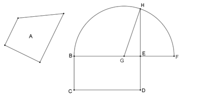
Figure 1: Elements, II.14.

In II.14, Euclid shows how to square a polygon. This construction crowns the theory of equal figures developed in propositions I.35–45; see (Błaszczyk 2018). In Book I, it involved showing how to build a parallelogram equal to a given polygon. In II.14, it is already assumed that the reader knows how to transform a polygon into an equal rectangle. The justification of the squaring of a polygon begins with a reference to II.5.

As for the proof technique, in II.11–14, Euclid combines the results of II.4–7 with the Pythagorean theorem by adding or subtracting squares described on the sides of right-angle triangles. Thus, II.5, 6 share the same scheme:

$$rectangle+\textit{square on}\ A=\textit{square on}\ B.$$

When applied, a right-angle triangle with a hypotenuse B and legs A, C is considered. Then, by I.47,

$$rectangle+\textit{square on}\ A=\textit{square on}\ A+\textit{square on}\ C.$$

By subtraction from both sides of the square on A, the equality characterizing II.11 and II.14 is obtained

$$rectangle=\textit{square on}\ C.$$

On the other hand, II.4, 7 share another scheme. In II.4, it is as follows

$$\textit{square on}\ A=\textit{square on}\ B+\textit{square on}\ C+2rectangles.$$

Addition to both sides another square gives the equality

$$\textit{square on}\ A+\textit{square on}\ D=\textit{square on}\ B+\textit{square on}\ D+\textit{square on}\ C+2rectangles.$$

D is a leg of two right-angle triangles: the first with another leg A and a hypotenuse E, the second with leg B and hypotenuse F. Thus, equality obtains

$$\textit{square on}\ E=\textit{square on}\ F+\textit{square on}\ C+2rectangles.$$

The use of II.7 starts with the equation

$$\textit{square on}\ A+\textit{square on}\ B=\textit{square on}\ C+2rectangles.$$

A square on the height AD of the triangle ABC is added to its both sides; see Fig. 2. The rest of the proof II.13 proceeds in a similar way.

Significantly, the accompanying diagram, next to sides of the triangle, features only the height AD. Thus, the point D represents the way the side BC is cut, namely at random. In this way, it makes a reference to II.7. The line AD represents the side of the square that is added to both sides of the above equation. All that illustrates our thesis, that although in II.11–14 Euclid relates squares and rectangles, the accompanying diagrams depict only the respective sides of the figures involved.

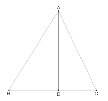
Figure 2: Elements, II.13.

2.3 In the search of patterns

References to II.4–7 follow a similar word pattern: For since the straight-line … has been cut … . Then comes a specification how new points are placed on the straight-line: in half (equally), at random (unequally), or a new line is added to the original one. Finally, a relation between resulting squares and rectangles established in the refereed proposition is reformulated due to new names of points.

For example, the respective part of II.14 is this: “since the straight-line BF has been cut equally at G, and unequally at E, the rectangle contained by BE, EF, together with the square on EG, is thus (ἄρα) equal to the square on GF”.

While II.5 states: “For let any straight-line AB have been cut equally at C and unequally at D. I say that the rectangle contained by AD, DB, together with the square on CD, is equal to the square on CB”.

Clearly, these statements differ only in names of points (for comparison, see Fig. 1 and Fig. 11).

In propositions II.1–8, depending on a distribution of cut points, a variety of squares and rectangles appears on the accompanying diagrams. Next to those represented on the diagrams, Euclid refers also to figures which are not represented on the diagrams; let us call them invisible figures. These are squares on and rectangles contained by some lines. Although the respective lines are represented on the diagrams, the related squares and rectangles are not. Indeed, whereas these invisible figures occur in the statements of propositions, Euclid’s proofs usually start with figures which are represented on the diagrams.

We recognized the following pattern in the procedures Euclid adopts in propositions II.1–8. Firstly, contrary to Book I, the diorisomos part of the proposition refers to figures not represented on the diagram. Secondly, in the kataskeuē, a geometric machinery is applied to construct figures represented on the diagram. Thirdly, in the apodeixis, a relation between figures which are represented and not represented on the diagram is determined. It is achieved by visual evidence, substitution rules, and the renaming of figures. In sections § 4–5, we will detail these issues, while section § 3 is dedicated to Euclid’s use of the terms square on and rectangle contained by.

As we proceed from II.1 to II.8, Euclid’s diagrams get more complicated: they depict more and more squares and rectangles. Then, in propositions II.9–10, they gain a new clarity. Indeed, II.9–10 explore the Pythagorean theorem in equating groups of squares, yet, the accompanying diagrams do not depict these squares. For example, II.10 reads: “For let any straight-line AB have been cut in half at C, and let any straight-line BD have been added to it straight-on. I say that the squares on AD, DB is double the squares on AC, CD” (see Fig. 3).

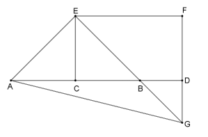
Figure 3: Elements, II.10.

Since the right-angle triangles ADG and AEG share the hypotenuse AG, squares on the legs of the first triangle, $AE$, $EG$, and on the legs of the second, $AD,DG$, are equal. The squares on $AE$ are $AC^{2},CE^{2}$; the squares on $EG$ are $FE^{2},FG^{2}$; and the squares on the legs of the second triangle are $AD^{2},DG^{2}$. Finally, Euclid determines equalities between squares to get the doubles of the squares, such as $2FE^{2}$ which is to be equal to the square on EG. Although the equality of line segments, $FG=EF$, is derived from I.6, the equality of respective squares, $FG^{2}=FE^{2}$, is based on an implicit rule: “since FG is equal to EF, the one on FG is equal to the one on EF”. In our interpretation, it is one of substitution rules discussed in section § 5.

Notice, that to justify the equality $FG^{2}=FE^{2}$, Euclid does not refer to the diagram. In fact, the accompanying diagram does not depict any square. It is also not the case, that this conclusion is taken for granted, since he provides a reason. Indeed, throughout Book II, Euclid reiterates the argument: since X is equal to Y, the square on X is equal to the square on Y.

Interestingly, the results II.9–10 could be obtained by dissection of the square on AB, in the case of II.9, and the square on AD, in the case of II.10, and then by the use of gnomons in a way similar to the proofs of II.5–8. Therefore, we view II.9–10 as introducing a new technique which combined with the results of lemmas II.4–7 is used in the proofs II.11–14.

The word pattern of references we identified above finds its diagrammatic counterparts in II.11–14. Starting from II.11, squares on are represented by lines, rectangles contained by – by lines with cut points. In II.11–14, diagrams look like ideograms rather than a simple composition of lines introduced throughout construction steps.

Let us focus on II.14 (see Fig. 1). The figure A and the rectangle BCDE refer to the theory of equal figures developed in Book I. The exposition of the line BF and the cut points G, E, refer to II.5. The semicircle BHF and the radius GH represent a new construction. The line EH represents the conclusion of the squaring of a polygon process.

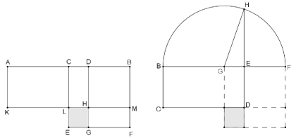
Figure 4: The scheme of application of II.5 in II.14.

In Fig. 4, we represent the way how II.5 is applied in II.14. The scheme of this application is as follows: Since the line BF is cut in half at G, and at random at E, by II.5, the equality obtains

$$rectangle\ BD+\textit{square on}\ GE=\textit{square on}\ GF.$$

Then, by I.47:

$$\textit{square on}\ GF=\textit{square on}\ GE+\textit{square on}\ HE.$$

Thus

$$rectangle\ BD+\textit{square on}\ GE=\textit{square on}\ GE+\textit{square on}\ HE.$$

By subtraction, the final equality obtains

$$rectangle\ BD=\textit{square on}\ HE.$$

Yet, instead of all these auxiliary lines that evoke the II.5 construction, Euclid’s original diagram is much simpler: it refers to II.5 by the way points G and E are located on the line EF. Note however, that Euclid reached this clarity due to the specific use of the term square on. Instead of the square on GH, he considers square on GF, instead of the square on GE, he considers another square – the gray one in Fig. 4, on the right. And that is why, in II.5, although he mentions the square on CD, he considers the square LEGH – the gray one in Fig. 4, on the left.

In sum, from the perspective of diagrams, Book II applies figures which are represented and not represented on the diagrams. These are squares on and rectangles contained by. II.9–10 apply line segments instead of squares on. II.11–14, besides lines representing squares on, apply also line segments with cut points instead of rectangles contained by.

3 Building-blocks of Euclid’s propositions of Book II

3.1 Individual vs abstract components of Euclid’s diagrams

There are two components of Euclid’s proposition: the text and the lettered diagram. The Greek text is linearly ordered – sentence follows sentence, from left to right, and from top to bottom. Diagrams consist of straight-lines and circles. The capital letters on the diagrams are located next to points; they name the ends of line segments, intersections of lines, or random points.

The text of the proposition is a schematic composition made up of six parts: protasis (stating the relations among geometrical objects by means of abstract and technical terms), ekthesis (identifying objects of protasis with lettered objects), diorisomos (reformulating protasis in terms of lettered objects), kataskeuē (a construction part which introduces auxiliary lines exploited in the proof that follows), apodeixis (proof, which usually proves the diorisomos’ claim), sumperasma (reiterating diorisomos). References to axioms, definitions, and previous propositions are made via the technical terms and phrases applied in prostasis.

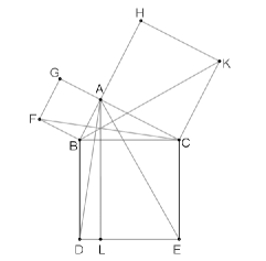
Figure 5: Elements, I.47.

In fact, it is the received account of Euclid’s propositions. For example, in proposition I.47, the protasis, ekthesis, and diorisomos are as follows (numerals in square brackets added, here they stand for subsequent parts of the proposition):

[1] “In a right-angle triangle, the square on the side subtending the right-angle is equal to squares on the sides surrounding the right-angle.

[2] Let ABC be a right-angled triangle having the right-angle BAC.

[3] I say that the square on BC is equal to the squares on BA and AC.”

Indeed, the triangle ABC as well as the squares constructed on lines BA and AC are all depicted on the accompanying diagram (see Fig. 5).

Yet, already in the first propositions of Book II, we observe a new phenomenon: figures mentioned in the diorisomos are not represented on the diagrams. Here are ekthesis and diorisomos of proposition II.2: “For let the straight-line AB have been cut, at random, at point C. I say that the rectangle contained by AB, BC together with the rectangle contained by BA, AC, is equal to the square on AB.”

On the accompanying diagram (see Fig. 6), we can see the lines AB, AC, and BC, however, neither the rectangle contained by AB, BC, nor the one contained byBA, AC is depicted on the diagram: line-segments AB, AC, and BC lay on the same straight line and do not contain a right-angle. Rectangles which are supposed to be formed by line segments not containing a right-angle occur in every proposition of Book II.

Furthermore, notice that in proposition II.14, Euclid shows how to “construct a square equal to a given rectilinear figure”. Although the accompanying diagram depicts a quadrilateral $A$, it is a symbol of a rectilinear figure rather than the individual object that is being studied in the proposition: it is not constructed, its vertices are not denoted by letters, and they are not involved in the constructions carried out in the proposition.

The diagram in proposition VI.31 plays an even more abstract role. The diorisomos part of VI.31 reads: “Let ABC be a right-angled triangle having the angle ABC a right-angle. I say that the figure on BC is equal to similar, and similarly described, figures on BA and AC.” Like figure A in proposition II.14, the rectangles on the sides of the triangle ABC are not constructed, they are not involved in the proof, and the proof does not rely on information read-off the diagram.

3.2 Rectangle contained by two straight-lines

Here is the crucial definition of Book II: “Any right-angled parallelogram is said to be contained by two straight-lines containing a right-angle”. Throughout the entire book, Euclid studies squares, rectangles, and triangles. The term right-angled parallelogram is applied only to rectangles, then it is reshaped to rectangle contained by two straight-lines. What, then, is the role of the term rectangle contained by two straight-lines? How does it differ from a simple rectangle?

Let us start with the most general concept, namely that of a figure. In Book I, Euclid defines a figure as follows: “A figure is that which is contained by some boundary or boundaries”. The term boundary applies to a circle only, boundaries apply to polygons. Hence, for example, a triangle is contained by three straight-lines, i.e., its sides. In other words, what we call a polygonal curve today is not considered to be a single line in the Elements – according to Euclid, it is a composition of lines.

In Book II, in addition to triangles, Euclid studies squares and rectangles. Definition I.22 clarifies these concepts. It reads: “And of quadrilateral figures: a square is that which is right-angled, and equilateral, a rectangle that which is right-angled but not equilateral”. The term parallelogram requires the concept of parallels and is not included in the list of definitions prefacing Book I. It occurs in proposition I.34 as parallelogrammic figure. Although not explicitly defined, it is clear what Euclid means: a parallelogram is a quadrilateral with two pairs of parallel sides (I.33 shows the existence of parallelograms). This term is closely related to Euclid’s theory of equal figures. Within this theory, in proposition I.44, Euclid shows how to construct a parallelogram when its two sides and an angle between them are given. Still, in Book II, all parallelograms are rectangles. What is, then, the reason for the term rectangle contained by two straight lines?

Firstly, this term is related to the ways figures are referred to in the text of the propositions, specifically, it is essential in protasis parts. Secondly, it plays an analogous role to the term square on a side: as the latter enables to identify a square with one side, the former enables to identify a rectangle with two sides with no reference to a diagram. Thirdly, since the terms square on a straight-line and rectangle contained by straight-lines are applied both to figures which are represented (visible) and not represented (invisible) on a diagram, these names make it possible to relate the visible and invisible figures. Due to substitution rules which we detail in section § 5, Euclid can claim that a rectangle contained by X,Y, which is not represented on the diagram, is contained by A, B, where segments A, B form a rectangle which is represented on the diagram.

3.2.1 Current interpretations of rectangle contained by

Within the so-called geometric algebra interpretation of Book II, all rectangles are represented by the formula $ab$, no matter whether lines $a,b$ contain a right-angle or not. Moreover, the term $ab$ is subject to some processing.

To be clear, we do not agree with the claim that this interpretation ignores the historical context by implying a multiplication of line segments. One may treat the terms $ab$, $a(b+c)$ as interpreting the phrases rectangle contained by lines $a,b$, or a rectangle contained by lines $a$ and $b,c$. Yet, when that the term $ab$ is applied in the same way to rectangles represented and not represented on a diagram, it blurs the essence of Book II.

John Baldwin and Andreas Mueller interpret a rectangle contained by X, Y as a rectangle of length X and height Y. They write: “This definition [II.1] allows us to study the areas of arbitrary rectangles by indexing each rectangle by its semi-perimeter and a cut point in that line” (Baldwin, Mueller 2019, 8). In proofs, instead of Y, they consider W such that W=Y, and lines X, W contain a right-angle. Thus, in fact, they reduce a rectangle contained by to a rectangle represented on a diagram. Still, they are the only authors that find Euclid’s definition “strange to modern ears”.

Ian Mueller tries yet another trick: “O(x,y) is used to designate a rectangle with arbitrary straight lines equal to $x$ and $y$ as adjacent sides” (Mueller 2006, 42). First of all, $\textbf{O}(x,y)$ denotes a rectangle and makes no difference between visible and invisible figures. For example, in Mueller’s formalization of II.2, there is no difference between O(AD,AC) and O(AB,AC), since $AB=AC$ (see Fig 6). By his notation alone, Mueller ignores the basic problem Euclid seeks to resolve in propositions II.1–8, namely the relation between a rectangle represented on the diagram, and one not represented on the diagram. As a result, he distorts Euclid’s original proofs, even though he can easily interpret the theses of his propositions.

Jeffrey Oaks provides a similar interpretation, as he writes in a commentary to proposition VI.16 of the Elements: “Here ‘the rectangle contained by the means’ in most cases will not be a particular rectangle given in position because the two lines determining it are not attached at one endpoint at a right angle. In fact, the sides determining rectangles cited in Greek works rarely satisfy Euclid’s definition at the beginning of Book II […]. Already in Proposition II.1 Euclid writes about ‘the rectangle contained by A, BC’ when the two lines may not be anywhere near each other. And the lines determining the rectangles cited in Proposition II.2 are absolutely not at right angles, since they are colinear. Propositions VI.16 and XI.34, like many propositions in Greek mathematics, are about the measures or sizes of geometric objects. ‘The rectangle contained by the means’ does not designate a particular rectangle given in position, but only the size of a rectangle whose sides are equal (we would say “congruent”) to those lines. Location and orientation of this rectangle relative to the other magnitudes in the diagram are undetermined and irrelevant to the argument. It is only the relative ‘measure’ that is intended” (Oaks 2018, 259).

At first, Oaks admits that not all rectangles contained by are featured on diagrams. Going beyond this observation, he links (invisible) rectangles with the concept of measure.

The above interpretations involve terms, figures and measure. We do not interpret the phrase rectangle contained by, but rather study its role in Euclid’s proofs. Eventually we view it as a proof technique not an object.

3.3 Identifying figures through letters and technical terms

In the Elements, Euclid adopts the following pattern of naming the figures featured on diagrams: squares and rectangles are, first of all, denoted by the letters located next to their vertices, they are also denoted by the letters which designate the diagonal. In proposition I.46, Euclid shows how to describe a square on a given straight-line. In the propositions that follow, squares are also identified by the phrase square on a straight-line, where the specific name of a line is given. We can illustrate this naming technique by referring to proposition I.47 (Fig. 5 represents the accompanying diagram).

Thus, in the text of the proposition, the square BDEC is also called the square on BC; the square on BA is also denoted by the two letters located on the diagonal, namely GB. Since the intersection of lines BC and AL is not named, rectangles that make up the square BDEC are named with two letters, as parallelogram BL and parallelogram CL.

In Book II, Euclid introduces yet another naming scheme for the rectangle: it is identified with its two sides and is called rectangle contained by, and the term is followed by the names of line-segments containing a right-angle.

All these naming rules – that is, by vertices, by a diagonal, square on, and rectangle contained by – apply to figures represented on the diagrams. Here, for example, is the text of proposition II.2 (Fig. 6 represents the accompanying diagram).

[1] “For let the straight-line AB have been cut, at random, at point C. I say that the rectangle contained by AB, BC together with the rectangle contained by BA, AC, is equal to the square on AB.

[2] For let the square ADEB have been described on AB, and let CF have been drawn through C parallel to either of AD or BE.

[3] So AE is equal to the AF, CE. And AE is the square on AB. And AF (is) the rectangle contained by BA, AC. For it is contained by DA, AC, and AD (is) equal to AB. And CE (is) by AB, BC. For BE (is) equal to AB. AB. Thus, by BA, AC, together with by AB, BC, is equal to the square on AB.”

Figure 6: Elements, II.2.

Thus, the square ADEB is also named the square on AB. Rectangle AF is also called the rectangle contained by DA, AC.

The phrases square on and rectangle contained by are also applied to figures not represented on diagram. In the text of proposition II.4, the term the square on AC occurs, although there is no such square on the accompanying diagram (see Fig. 8). Also in this proposition, the term rectangle contained by AC, CB occurs, although there is no such rectangle on the accompanying diagram.

In fact, rectangles contained by straight-lines lying on the same line and not containing a right-angle are common in Book II. Whether represented on diagrams or not, as a rule, they are contained by individual straight-lines. However, proposition II.1 represents a unique case in this respect. Therein, Euclid considers rectangles contained by A, BD, and A, DE, and A, EC (see Fig. 7). They are to be rectangles contained by BG, BD, by DK, DE, and by EL, EC respectively. Rectangles contained by A, BD, by A, DE, and A, EC are neither represented on the diagram, nor contained by individual line-segments: line A, considered as a side of these rectangles, is not an individual line.

To be clear, the relation between rectangles, contained on the one hand by A, BD, and on the other by BG, BD, is not an equality: it is stated that the former is the rectangle contained by BG, BD. The relevant part of the proposition reads: “BK is by A, BD. For it is contained by GB, BD, and BG is equal to A”. Here, BK is represented on the diagram, and Euclid claims that it is contained by BG, BD, which is simply another name of the rectangle BK. Still, Euclid also claims that BK is contained by A, BD, while the later rectangle is not represented on the diagram. Thus, the relation between figures represented and not represented on a diagram is founded on substitution and renaming rules. We will explicate these rules in section § 5. In general, Euclid engages a bunch of tricks to establish an equation between a rectangles contained by and a figures represented on a diagram.

Interestingly, Euclid never refers to proposition II.1. Moreover, its result, when viewed from the modern perspective, is reiterated in propositions II.2 and II.3. Hence, it seems that its role is to demonstrate the substitution rules which are applied throughout the rest of Book II, rather than to present a specific geometrical statement. All that is required to analyze these rules are propositions II.1–II.4. From the perspective of substitution rules, proposition II.1 introduces them, then proposition II.2 applies them to rectangles contained by, and proposition II.4 – to squares on. Proposition II.4 involves yet another object, namely the so-called complement. It shows how to apply the substitution rules to these objects.

From the perspective of represented vs not represented figures, proposition II.2 equates figures which are represented, on the one side, and not represented, on the other, while proposition II.3 equates figure not represented, on the one side, and figures represented and not represented, on the other side, proposition II.4 introduces yet another operation on figures which are not represented, as it includes an object called twice rectangle contained by, where the rectangle is not represented on the diagram.

3.3.1 Algebraic view on propositions II.1–3

Without paying attention to Euclid’s vocabulary, specifically to the terms square on and rectangle contained by, one cannot find a reason for propositions II.2 and II.3. Thus, Bartel van der Waerden in (Waerden 1961) considers them as special cases of II.1. Similarly, Robin Hartshorne, in the Appendix to (Hartshorne 2000), includes statements of “the most frequently quoted results” of the Elements. Regarding Book II, he refers to proposition II.1, then skips to II.4.

From the modern perspective, especially when the diorismos of Euclid’s proposition is stylized as an algebraic formula, such an interpretation seems reasonable. For, when II.1 is rendered as $a(b+c+d)=ab+ac+ad$, then II.2 is $a^{2}=ab+ac$, given $a=b+c$, and II.3 is $a(b+a)=ab+a^{2}$. Indeed, II.2 and II.3 follow from II.1 by suitable substitutions. In fact, however, proposition II.1 is never quoted in the Elements, and due to the role of line A it is a unique proposition in the entire Elements.

4 Schemes of propositions II.1 to II.4

In this section, we provide detailed analysis of propositions II.1 to II.4. They aim to reveal non-geometrical rules which enable to relate figures represented and not represented on the diagrams.

Here is the text of proposition II.1, starting with the diorismos:

Diorismos “Let A, BC be the two straight-lines, and let BC, be cut, at random, at points D, E. I say that the rectangle contained by A, BC is equal to the rectangles contained by A, BD, by A, DE, and, finally, by A, EC.”

Kataskeuē  “For let BF have been drawn from point B, at right angles to BC, and let BG be made equal to A […].”

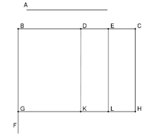
Figure 7: Elements, II.1.

“[1] So BH is equal to BK, DL, EH. [2] And BH is by A, BC. For it is contained by GB, BC, and BG is equal to A. [3] And BK (is) by A, BD. For it is contained by GB, BD, and BG is equal to A. [4] And DL is by A, DE. For DK, that is to say BG, is equal to A. [5] Similarly, EH (is) also by A, EC. [6] Thus, by A, BC is equal to by A, BD, by A, DE, and, finally, by A, EC.”

Now, we present this proposition in a more schematic form. In what follows, symbol $A\times BC$ stands for the phrase “rectangle contained by A, BC”, while $BH\,\pi\,GB\times BC$ stands for the phrase “BH is contained by GB, BC”.

Diorismos

$$A\times BC=A\times BD,\,A\times DE,\,A\times EC.$$

Kataskeuē $BF\perp BC,\ BG=A$; $GH\parallel BC$; $DK,EL,EH\parallel BG$.
Apodeixis

$${\color[rgb]{1,0,0}BH=BK,DL,EH}$$

$${\color[rgb]{0,0,1}BH\,\pi\,GB\times BC},\ BG=A \xrightarrow[]{} {\color[rgb]{.5,0,.5}BH\,\pi\,A\times BC}$$

$${\color[rgb]{0,0,1}BK\,\pi\,GB\times BD},\ BG=A \xrightarrow[]{} {\color[rgb]{.5,0,.5}BK\,\pi\,A\times BD}$$

$$DK=BG=A \xrightarrow[]{} {\color[rgb]{.5,0,.5}DL\,\pi\,A\times DE}$$

$$\xrightarrow[]{} {\color[rgb]{.5,0,.5}EH\,\pi\,A\times EC}$$

$$\xrightarrow[]{} {\color[rgb]{1,0,1}A\times BC=A\times BD,\,A\times DE,\,A\times EC}.$$

(1) The formula in red interprets sentence [1]. It is a simple statement with no justification and the starting point of the whole argument. Since the figures involved are represented on the diagram, we interpret it as based on purely visual evidence.

All of the rectangles mentioned in the diorismos are not represented on the diagram. Therefore, we are to explain how, starting from the relation between the figures represented on the diagram, Euclid gets the relation between figures not represented on the diagram.

(2) The next line in the apodeixis scheme interprets sentence [2]. The formula in blue stands for the phrase “BH […] is contained by GB, BC”. It is one of the three possible names for a rectangle represented on a diagram. Thus, it is a result of renaming figures rather than a geometrical or logical relation. Hereafter, formulas resulting from renaming will be represented in blue.

The equality $BG=A$ follows from the construction part of the proposition. Yet, the most puzzling is the phrase “BH is by A, BC”. We interpret it as a result of substituting A to the formula $BH\,\pi\,BG\times BC$ in place of BG. Arguments of this kind are applied all throughout Book II. The relation between the rectangle BH, and the one contained by A, BC is by no means an equality; the word pattern “BH is by A, BC” is systematically used by Euclid. Let us represent formulas obtained by this type of substitution in violet.

(3) In sentence [3], Euclid reiterates the previous argument.

(4) In sentence [4], Euclid skips supposition ${\color[rgb]{0,0,1}DL\,\pi\,DK\times DE}$ and notes the equalities $DK=BG=A$. They can be justified by Common Notion 1.

(5) In sentence [5], Euclid skips arguments relying on substitution and CN1, and simply states the result. It is a way of shortening repeated arguments, typical of Euclid.

(6) In sentence [6], with ἄρα, Euclid reaches the equality between invisible rectangles. We interpret this step as a result of another substitution rule: in the equality starting in apodeixis, $A\times BC$ is substituted for BH, then $A\times BD$ is substituted for BK, etc.

Let us represent the equality obtained by this type of substitution, i.e., substitutions for equality, in magenta.

The arrow $\rightarrow$ in the scheme stands for a conjunction, usually it is γάρ. It is by no means suggested to be a logical implication.

II.2 (see Fig. 6)

In the below scheme, the term $AB^{2}$ stands for the phrase “the square on AB”. Thus, for example, $AE\ is\ AB^{2}$ interprets the phrase “AE is the square on AB”, or “AE is on AB”.

Diorismos

$$AB\times BC,BA\times AC=AB^{2}.$$

Apodeixis

$${\color[rgb]{1,0,0}AE=AF,CE}$$

$${\color[rgb]{0,0,1}AE\ is\ AB^{2}}$$

$${\color[rgb]{0,0,1}AF\,\pi\,DA\times AC},\ AD=AB \xrightarrow[]{} {\color[rgb]{.5,0,.5}AF\,\pi\,BA\times AC}$$

$$BE=AB \xrightarrow[]{} {\color[rgb]{.5,0,.5}CE\,\pi\,AB\times BC}$$

$$\xrightarrow[]{} {\color[rgb]{1,0,1}BA\times AC,AB\times BC=AB^{2}}.$$

Lines (3) and (4) of the apodeixis scheme, represent, again, typical of Euclid way of shortening repeated arguments: in line (4), Euclid skips the premise CE is between CF, BC.

In this proposition, the diorismos equates the figure represented on the diagram, that is, the square on AB, with figures not represented on the diagram, namely rectangles contained by AB, BC, and AB, AC.

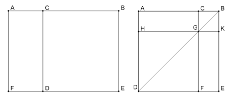
Figure 8: Elements II.3 (left) and II.4 (right).

II.3 (see Fig. 8)

Diorismos

$$AB\times BC=AC\times CB,\,BC^{2}.$$

Apodeixis

$${\color[rgb]{1,0,0}AE=AD,\,CE}$$

$${\color[rgb]{0,0,1}AE\,\pi\,AB\times BE},\ BE=BC \xrightarrow[]{} {\color[rgb]{.5,0,.5}AE\,\pi\,AB\times BC}$$

$$DC=CB \xrightarrow[]{} {\color[rgb]{.5,0,.5}AD\,\pi\,AC\times CB}$$

$${\color[rgb]{0,0,1}DB\ is\ CB^{2}} \xrightarrow[]{} {\color[rgb]{1,0,1}AB\times BC=AC\times CB,\,BC^{2}}.$$

Here, the square CE is also named by the second diagonal, as DB. Apart from this fact, this apodeixis is similar to the previous one.

In this proposition, Euclid equates the figure not represented on the diagram, $AB\times AC$, with figures both represented and not represented on the diagram, $AC\times CB,\,BC^{2}$.

Proposition II.1–3 share the same word patterns clearly represented by the colors of terms in our schemes. Since there are no explicit references to these propositions in the rest of Book II, we treat them as introducing a technique of dealing with figures which are not represented on diagrams.

With II.4, we pass to a proposition which will be referred to in the following propositions.

II.4 (see Fig. 8)

Diorismos

$$AB^{2}=AC^{2},\,CB^{2},\,2AC\times CB.$$

Apodeixis.

$${\color[rgb]{0,0,1}CGKB\ is\ CB^{2}}$$

$${\color[rgb]{0,0,1}HF\ is\ HG^{2}},{\color[rgb]{.5,0,.5}HF\ is\ AC^{2}} \xrightarrow[]{} HF,\,KC\ are\ AC^{2},\,CB^{2}$$

$$GC=CB \xrightarrow[]{} {\color[rgb]{.5,0,.5}AG\,\pi\,AC\times CB}$$

$$AG=GE \xrightarrow[]{} {\color[rgb]{1,0,1}GE=AC\times CB}$$

$$\xrightarrow[]{} AG,GE=2AC\times CB$$

$$HF,CK\ are\ AC^{2},CB^{2} \xrightarrow[]{} HF,\,CK,\,AG,\,GE=$$

$$=AC^{2},\,BC^{2},\,2AC\times CB$$

$${\color[rgb]{1,0,0}HF,\,CK,\,AG,\,CE=ADEB},$$

$${\color[rgb]{0,0,1}ADEB\ is\ AB^{2}} \xrightarrow[]{} {\color[rgb]{1,0,1}AB^{2}=AC^{2},\,CB^{2},\,2AC\times CB}.$$

In this proposition, Euclid equates the figure represented on the diagram, $AB^{2}$, with figures represented, $CB^{2}$, and not represented on the diagram, $AC^{2}$, $2AC\times CB$. A new component is the square on AC which is not represented on the diagram. Next, “twice the rectangle contained by AC, CB” means that Euclid handles not represented rectangles the same way as represented ones.

Formula $HF\ is\ HG^{2},HG^{2}\ is\ AC^{2}$ interprets the following phrase: “HF is also a square. And it is on HG, that is to say AC”. We formalize it like this:

$$HF\ is\ HG^{2},HF=AC\rightarrow HF\ is\ AC^{2}.$$

Thus, from the adopted perspective, it is a substitution rule applied to the square on, analogous to the one applied to the rectangle contained by. That is why it is highlighted in violet.

Now, let us focus on the lines (3) and (4) of the apodeixis scheme. They interpret the following part of Euclid’s proof: “AG is equal to GE. And AG is contained by AC, CB. For GC is equal to CB. Thus, GE is also equal to the one by AC, CB”. The equality $AG=GE$ follows from proposition I.43. $AG\,\pi\,AC\times CB$ is the result of the substitution rule we already identified. The conclusion “GE is also equal to the one by AC, CB” is the result of a substitution to the equality.

In regard to the term $AG,GE=2AC\times CB$, we cannot provide a clear justification for this conclusion. The same applies to the conclusion

$$HF,\,CK,\,AG,\,GE=AC^{2},\,BC^{2},\,2AC\times CB.$$

Although we could justify it by using logical tricks, it is not Euclid’s style to conceal complicated rules and explicate simple ones. It seems to be a puzzle Euclid could not resolve.

The formula in red interprets the following sentence: “HF, CK, AG, GE are the whole ADEB”. Like in previous cases, we take it to be justified by visual evidence. From a logical point of view, it could be the starting point of this proof.

4.0.1 David Fowler on proposition II.4

In regard to propositions II.1–8, Fowler writes: “In all of these propositions, almost all of the text of the demonstrations concerns the construction of the figures, while the substantive content of each enunciation is merely read off from constructed figures, at the end of the proof, as in lines 49 to 50 of II.4, the proposition just considered” (Fowler 2003, 69)

Our schemes evidence that arguments read off the diagrams are staring points of the proofs II.1–3. In II.4–8, they are at the end of proofs. However, the enunciations of propositions II.1–8 concern figures which are not represented on the diagrams, therefore the essential arguments can not be read off the diagrams.

Commenting on the final lines of the proof II.4, Fowler writes:

Therefore the four areas HF, CK, AG, GE are equal to the square on AC, CB, and twice the rectangle by AC, CB,

and the fact that this gives a decomposition of the square, the ostensible point of the proposition, is merely stated (lines 49 to 50):

But HF, CK, AG, GE are the whole ADEB, which is the square on AB” (Fowler 2003, 69)

The point is that HF, CK, AG, GE give the decomposition of the square ADEB, not “AC, CB, and twice the rectangle by AC, CB”.

4.0.2 Ian Mueller’s interpretation again

Interestingly, the equality $GE=AC\times CB$ follows from the equality $AG=GE$ rather than from the rule:

$$A\,\pi\,C\times D,\ C=E,\ D=F,\ B\,\pi\,E\times F\rightarrow A=B.$$

This alternative argument is obvious within the so-called geometric algebra, as well as Mueller’s interpretation (see § 3.2 above). More specifically, within Mueller’s interpretation the equality (congruence) obtains

$$x=A,y=B\Rightarrow\textbf{O}(x,y)\simeq\textbf{O}(A,B).$$

However, we have not identified this rule in Book II. On the contrary, proposition II.4 exemplifies different reason, namely

$$A\,\pi\,C\times D,\ A=B\rightarrow B=C\times D.$$

In words, since we know that figures A and B are equal and one of them is contained by C, D, then the other is also contained by C, D. It means, that the equality established within the theory of equal figures is more fundamental than the relation contained by. In a way, Euclid aims to introduce rectangles contained by into equalities of non-congruent figures. Within Mueller’s interpretation the equality between rectangles follows from a relation contained by.

5 Non-geometrical rules in Book II

Four colors in or schemes of Euclid’s propositions correspond to three groups of rules: visual evidence (red), renaming (blue) and substitutions (violet and magenta). In this section we scrutinize these rules.

5.1 Visual evidence

It is standard to identify two meanings of equality of figures in the Elements – congruence and the equality of non-congruent figures. The congruence of figures is usually linked to the idea of coinciding figures involved in Common Notion 4. It is also commonly assumed that the idea of coinciding figures plays a crucial role in proposition I.4. But the superposition of figures presupposes (rigid) motion.

The statements in red in our schemes are so simple that they do not engage any other concepts. If any needed justification, CN4 would be a good choice. Although such an interpretation finds no textual corroboration, there are no significant differences between the claim that CN4 is founded on visual evidence and the claim that statements in red are justified by CN4. In fact, Euclid provides no arguments for these statements.

5.2 Overlapping figures

At first, the range of visual evidence is obvious: it justifies the equality of a figure and their dissection parts, which are squares and rectangles. Yet, as we proceed further, in propositions II.5–8, Euclid extends its power to another cases. In II.5, the gnomon NOP is taken together with the square LG and Euclid declares that they form the square CEFG: “the gnomon NOP and the square LG are the whole square CEFB” (see Fig. 11). We interpret it as an equality based on visual evidence, $NOP,LG=CEFB$.

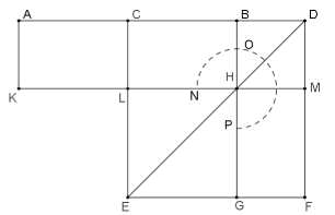
Figure 12: Elements II.6.

In the next proposition, the diagram is the same as regards the gnomon and its complementing square. This time, instead of the square LG, Euclid adds the square on BC to the gnomon NOP (see Fig. 12). His argument is this: since $LG=BC^{2}$, then $NOP,BC^{2}=CEFB$. However, while the equality $NOP,LG=CEFD$ is visually obvious, the equality $NOP,BC^{2}=CEFB$ requires other kind of justification, as $BC^{2}$ is not represented on the diagram. If we add an auxiliary line to represent the square on BC, we will get overlapping figures. Thus, the status of the equality $NOP,BC^{2}=CEFB$ is not as obvious as $NOP,LG=CEFB$ in II.5.

In II.7, Euclid goes a bit further in terms of abstraction. He explicitly considers overlapping figures: the rectangle AF, and the square CE. He claims that they together form the gnomon KLM and the square CF: “but AF, CE are the gnomon KLM and the square CF” (see Fig. 9). Here is the scheme of the proof.

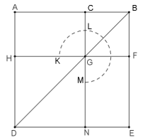
Figure 9: Elements II.7.

Diorismos

$$AB^{2},BC^{2}=2AB\times BC,CA^{2}.$$

Apodeixis

$$AG=GE \xrightarrow[CN3]{} AG,CF=GE,CF$$

$$AF=CE \xrightarrow[]{} AF,CE=2AF$$

$$\xrightarrow[]{} {\color[rgb]{1,0,0}KLM,CF=2AF}$$

$$BF=CB \xrightarrow[]{} {\color[rgb]{1,0,1}2AF=2AB\times BC}$$

$${\color[rgb]{0,0,1}DG\ is\ AC^{2}} \xrightarrow[]{} KLM,DG,GB=2AB\times BG,AC^{2}$$

$${\color[rgb]{1,0,0}KLM,DG,GB=ADEB,GB} \xrightarrow[]{} ADEB,GB=2AB\times BG,AC^{2}$$

$$\xrightarrow[]{} AB^{2},BC^{2}=2AB\times BG,AC^{2}.$$

Here, the red suggest that the respective formulas are based on visual evidence. Yet, since rectangles AF and CE overlap, i.e., share the square CF, they do not represent the same kind of evidence as red formulas in propositions II.1–4.

In II.8, Euclid’s considers even more complicated configuration of overlapping figures. Below we present the scheme of the key step (see Fig. 10).

$$DK=CK=GR=RN \xrightarrow[]{} DK,CK,GR,RN=4CK$$

$$AG=MQ=QL=RF \xrightarrow[]{} AG,MQ,QL,RF=4AG$$

$$\xrightarrow[]{} {\color[rgb]{1,0,0}DK,CK,GR,RN,AG,MQ,QL,RF=STU}$$

$$\xrightarrow[]{} {STU=4AK}.$$

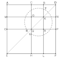
Figure 10: Elements II.8.

The red formula interprets the following sentence: “the eight, which comprise the gnomon STU”. Due to an implicit step

$$DK,CK,GR,RN,AG,MQ,QL,RF=4AK,$$

Euclid managed to bypass an explicit reference to overlapping figures. The missing step could be like this: AG=MQ=QL, CK=GR, then AK=MR=GL. However, here the square GR is counted twice. Thus, the square GR could be moved to cover the square DK. Argument of this kind characterize the so-called dissection proofs, for example, the famous Chinese proof the Pythagorean theorem. Significantly, Euclid does not apply dissection combined with a translation.

Another option could be a reference to CN2, namely: since AG=QL and CK=DK, then AG, CK= QL, DK. However, as a rule, Euclid does not apply CN2 when the resulting figure is not connected, i.e., it does not make a whole. Nevertheless, it is possible when the resulting figures overlap.

With the use of modern technology, overlapping figures are handled with shades, or colors. Yet, these are textbooks tricks. Foundational studies seek to eliminate overlapping figures, as we demonstrate in the next section.

5.2.1 Hilbert-style account of visual evidence

Within Hilbert’s tradition of reading the Elements, the congruence of line segments, angles, and triangles is covered by their respective axioms, Euclid’s proposition I.4 specifically is an axiom in the Hilbert system. Euclid’s theory of equal figures is covered by the idea of the content of a figure.

Robin Hartshorne develops Hilbert’s idea of content further to the modern concept of measure. Regarding Euclid’s theory of equal figures, he writes: “Looking at Euclid’s theory of area in Books I–IV, Hilbert saw how to give it a solid foundation. We define a notion of equal content by saying that two figures have equal content if we transform one figure into the other by adding and subtracting congruent triangles” (Hartshorne 2000, 195).

Indeed, figures involved in equalities in red also have equal content in the Hilbert-Hartshorne system. However, a justification is far from obvious. Let us take, for example, proposition II.2 and Euclid’s statements AE=AF, CE. Hartshorne’s definition of a figure reads: “A rectilinear figure […] is a subset of the plane that can be expressed as a finite non-overlapping union of triangles” (Hartshorne 2000, 196). AE, on the one hand, and AF, CE, on the other, meet the requirements of this definition. The next definition is this: “Two figures $P,P^{\prime}$ are equidecomposable if it possible to write them as non overlapping unions of triangles

$$P=T_{1}\cup....\cup T_{n},\ \ P^{\prime}=T^{\prime}_{1}\cup....\cup T^{\prime}_{n},$$

where for each $i$, the triangle $T_{i}$ is congruent to the triangle $T^{\prime}_{i}$” (Hartshorne 2000, 197). Then, the definition of equal content follows: “Two figures $P,P^{\prime}$ have equal content if there are other figure $Q,Q^{\prime}$ such that: (1) $P$ and $Q$ are not overlapping, (2) $P^{\prime}$ and $Q^{\prime}$ are not overlapping, (3) $Q$ and $Q^{\prime}$ are equidecomposable, (4) $P\cup Q$ and $P^{\prime}\cup Q^{\prime}$ are equidecomposable” (Hartshorne 2000, 197).

Thus, the proof that AE and AF, CE have equal content would be the same as the proof of the reflexibility of the relation have equal content, as if AE and AF, CE were the same figures. In fact, from the perspective of set theory, which makes the basis of the Hartshorne system, $AE=AF\cup CE$. However, it is not enough. To decide that AE and AF, CE are equidecomposable, we not only have to cover both sides with the same triangles, we also need to add to both sides another figure Q. This peculiar step is the price for the solid account of Euclid’s visual evidence.

Now, let us take the rectangle contained be BA, AC. Given Hartshorne’s definition, it is not a figure at all. Therefore $BA\times AC$ cannot be studied within this theory.

In sum, within the Hartshorne system, one can provide conceptually complicated proof of a statement which is obvious in the Elements. However, a complete reconstruction of Book II is impossible since there is no counterpart of the concept rectangle contained by. Hartshorne overestimates his system when he claims that “In Book II, all of the results make statements about certain figures having equal content to certain others, and all of these are valid in our framework” (Hartshorne 2000, 203) In fact, his system does not enable to identify the real problems of Book II, that is, a relation between the represented and not represented figures.

In modern system of geometry, the measure of a figure, that is a real number, plays the role of figures which are not represented.

5.3 Renaming

Our schemes of Euclid’s propositions clearly expose the role of the names of figures in the analyzed arguments. Rectangles represented on the diagrams are named by their vertices, diagonals, and as contained by two line segments. Squares represented on the diagrams, similarly, are named by their vertices, diagonals, and as a square on a side. Figures which are not represented get only one name: it could be a rectangle contained by two lines, or a square on a line. Thus, the most important factor is that figures represented on the diagrams can also be named rectangle contained by, or square on. Then, due to substitution rules, they can be related to figures not represented on the diagrams.

In a model example, in proposition II.2 (see Fig. 6), the rectangle AF is represented on the diagram and gets the name contained by DA, AC. Segments DA, AC are represented on the diagram and contain the right-angle. Then, Euclid claims that “AF is contained by BA, AC”, for “AD is equal to AB”. However, the rectangle contained by BA, AC is not represented on the diagram. Moreover, these lines do not contain a right-angle. That is why, in our scheme, $AF\,\pi\,DA\times AC$ is represented in blue – it is simply a new name for a visible figure. Nevertheless, to turn $AF\,\pi\,DA\times AC$ into $AF\,\pi\,BA\times AC$ a substitution rule is needed, namely rule (3) presented in the next section.

5.4 Substitution

First of all, observe that it is not explicit that the relation contained by is commutative, therefore we will not apply the following rule $X\times Y=Y\times X$. Euclid also does not apply this seemingly obvious rule: if $X=U,Y=W$, then $X\times Y=U\times W$.

The first substitution rule, applied all throughout Book II, is the one denoted in violet in our schemes. It is as follows

$$X\,\pi\,Y\times V,\ Y=U\Rightarrow X\,\pi\,U\times V.$$ (1)

The point is, while $X$ and $Y\times V$, as well as $Y$, $V$, and $U$, are represented on the diagram, $U\times V$ is not. The following line from the scheme of proposition II.2 exemplifies this rule:

$$AF\,\pi\,DA\times AC,\ AD=AB\rightarrow AF\,\pi\,AB\times AC.$$

A similar rule applies to square on, namely

$$X=Y^{2},Y=U\Rightarrow X=U^{2}.$$ (2)

The point is, while the square $X$ and its side $Y$ are represented on a diagram, the square $U^{2}$ is not, although the side $U$ is represented.

We exemplify it by an argument from proposition II.4:

$$HF\ is\ HG^{2},\ HG=AC\rightarrow HF\ is\ AC^{2}.$$

This formula interprets the following phrase: “HF is also a square. And it is on HG, that is to say on AC”. Results based on this rule could be also achieved by a reference to proposition I.36. Yet, it would require introducing another point and an extra construction. Significantly, Euclid does not refer to I.36 in this context.

Finally, the rule concerning substitution to an equality; in our schemes it is represented in magenta. It is as follows:

$$X=Y,\ X\,\pi\,U\times W\Rightarrow U\times W=Y.$$ (3)

Since the relation of equality is symmetric, by applying this rule, we can also get the following result

$$X=Y,\ \ X\,\pi\,U\times W,\ Y\,\pi\,Z\times V\Rightarrow U\times W=Z\times V.$$

Thus, in proposition II.1, the starting point is this

$$BH=BK,DL,EH.$$

Then, by rule (1), we get the following results

$$BH\,\pi\,A\times BC,\ BK\,\pi\,A\times BD,\ DL\,\pi\,A\times DE,\ EH\,\pi\,A\times EC.$$

Finally, by rule (3), we reach the conclusion

$$A\times BC=A\times BD,\ A\times DE,\ A\times EC.$$

To be clear, these substitution rules apply to the relation contained by rather than an equality of rectangles contained by. In II.11 and II.14, we can find a rectangle contained by equal to a square represented on the diagram. The equality is achieved by rule (3). Another way to equate rectangle contained by and a figure represented on a diagram is by combining the Pythagorean theorem and Common Notion 2. This trick is applied in II.11–14. In other words, whenever a rectangle contained by is equal to another figure, it is not a straightforward relation.

6 From visible to invisible and backward

In this section, we study the use of propositions II.5, 6 in II.11, 14, and show how through the technique of rectangles contained by Euclid has managed to establish a relation between visible figures. From a methodological point of view, he applies results obtained in one domain to determine results in another domain. It is like a factorization of real polynomial by its factorization in the domain of complex numbers, or, finding a solution to a problem in the domain of hyperreals, then, with its standard part, going back to the domain of real numbers.

6.1 Propositions II.5–6

Propositions II.5, 6 are often discussed in the literature, as scholars seek to provide a reason for including these seemingly twin propositions into Book II. First, we show how the substitution rules impact the interpretation of these propositions.

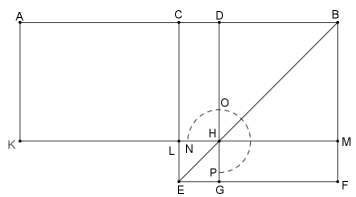
Figure 11: Elements II.5.

Viewed in terms of construction, they look alike (see Fig. 11 and 12). Line AB is cut in half at C, then point D is placed between C and B, or on the prolongation of AB. Yet, their protasis parts differ in wording: in the first case, Euclid considers equal and unequal lines, in the second case, the whole line and the added line. Still, when we proceed to their diagrams and diorismos, they are again similar. Moreover, their proofs apply the same trick: at first, Euclid shows that a rectangle is equal to a gnomom, then he adds a square that complements the gnomon to a bigger square.

We present a scheme of proposition II.5 starting from when it is established that the rectangle AH is equal to the gnomon NOP.

II.5

Diorismos

$$AD\times DB,CD^{2}=CB^{2}.$$

Apodeixis

$$... \xrightarrow[]{} AH=NOP$$

$$DH=DB \xrightarrow[]{} {\color[rgb]{.5,0,.5}AH\,\pi\,AD\times DB}$$

$$\xrightarrow[]{} {\color[rgb]{1,0,1}NOP=AD\times DB}$$

$${\color[rgb]{.5,0,.5}LG=CD^{2}} \xrightarrow[CN2]{} NOP,LG=AD\times DB,CD^{2}$$

$${\color[rgb]{1,0,0}NOL,LG=CEFB}$$

$${\color[rgb]{0,0,1}CEFB\ is\ CB^{2}} \xrightarrow[]{} AD\times DB,CD^{2}=CB^{2}.$$

Similarity, we schematize Euclid’s proof of the next proposition starting from the conclusion: the rectangle AM is equal to the gnomon NOP.

II.6

Diorismos

$$AD\times DB,CB^{2}=CD^{2}.$$

Apodeixis

$$... \xrightarrow[]{} AM=NOP$$

$$DM=DB \xrightarrow[]{} {\color[rgb]{.5,0,.5}AM\,\pi\,AD\times DB}$$

$$\xrightarrow[]{} {\color[rgb]{1,0,1}NOP=AD\times DB}$$

$${\color[rgb]{.5,0,.5}LG=BC^{2}} \xrightarrow[]{} AD\times DB,BC^{2}=NOP,BC^{2}$$

$$NOL,BC^{2}=CEFB$$

$${\color[rgb]{0,0,1}CEFD\ is\ CD^{2}} \xrightarrow[]{} AD\times DB,BC^{2}=CD^{2}.$$

In both propositions, figures not represented on the diagrams are to be equal to the squares represented on the diagrams. Euclid’s job is to show that these not represented are equal to some figures represented on the diagrams. The gnomon NOP plays the crucial role in that process.

When one pays no attention to the distinction between figures in terms of the representation on the diagram, these proofs are alike. However, in II.5, when Euclid takes together the square LG and the gnomon NOP, they make a figure represented on the diagram. Thus, equality $NOP,LG=CEFB$ is based on visual evidence. In II.6, Euclid adds the square on BC, which is not represented on the diagram, to the gnomon NOP. Thus, equality $NOP,BC^{2}=CEFB$ can not be based on visual evidence here. In fact, Euclid skips an argument justifying this step. Thus, the second proof is more abstract.

Let us consider the sequence of propositions II.5–8 from the perspective of visible and invisible figures. In II.5, the equality $NOL,LG=CEFB$ is based on visual evidence. In II.6, the equality $NOL,BC^{2}=CEFB$ is not so obvious, yet in the company of II.5 it is almost the same. In II.7, Euclid adds to the gnomon KLM, the complementing square DG and another one placed on the same diagonal DB. These figures are represented on the diagram, yet the equality $KLM,DG,GB=ADEB,GB$ involves overlapping figures. In II.8, Euclid considers overlapping figures but not represented on the diagram. It is typical of Euclid sequence of micro-steps, similar, e.g. to the first propositions in his theory of equal figures, when he considers parallelograms on the same base, then on equal bases (I.35–36), triangles on the same base, then on equal bases (I.37–38). Therefore, when II.5, 6 are considered in isolation, they provide almost the same result. When viewed in a bigger picture, they pave a way to a more abstract diagrams.

6.1.1 Van der Waerden’s and Corry’s interpretations

Here is van der Waerden’s interpretation: “We see therefore, that, at bottom, II 5 and II 6 are not propositions, but solutions of problems; II 5 calls for the construction of two segments x and y of which the sum and product are given, while in II 6 the difference and the product are given. The applications in the Elements themselves are consistent with this view” (Waerden 1961, 121).

In his view, II.5 and II.6 are two propositions for one formula, namely $(\frac{x+y}{2})^{2}=xy+(\frac{x-y}{2})^{2}$, which is why they need to be interpreted as solutions of problems rather than mere propositions. To illustrate his idea, van der Waerden interprets proposition II.11 as the solving of a specific equation. Yet, II.11 also allows a standard, say a Hilbert-style interpretation, where II.6 is referred to in order to get the result $CF\times FA,AE^{2}=EF^{2}$.

We interpret II.6 as lemma which is applied in II.11, while II.11 we view as the crucial step in Euclid’s construction of dodecahedron – a regular solid foreshadowed in Plato’s Timaeus.

Corry’s interpretation is as follows: “if we remain close to the Euclidean text we have to admit that, particularly in the cases of II.5 and II.6, both the proposition and its proof are formulated in purely geometric terms. There are no arithmetic operations involved, and surely there is no algebraic manipulation of symbols representing the magnitudes involved. The entire deduction relies on the basic properties of the figures that arise in the initial construction or that were proved in previous theorems (which in turn were proved in purely geometric terms)” (Corry 2013, 647).

Our schemes clearly show that Euclid’s deduction only partly relies on constructed figures. Euclid’s results in Book II also concern figures which are not represented on diagrams, and not constructed.

6.2 The use of II.5–6

We present propositions II.5–6 as lemmas. Indeed, II.5 is applied in II.14, II.6 – in II.11. The word pattern of these references is the same: Euclid simply repeats the ekthesis with new names of the respective points. In regard to II.5 it is: “For let any straight-line AB have been cut – equally at C, and unequally at D”. As for II.6 it is: “For since the straight-line AC has been cut in half at E, and FA has been added to it”. In this way, the applied propositions are identified by the patterns of the cut points: with II.5 it is equally and unequally, with II.6 – at half and a line added. This style of references compels Euclid to prove two propositions. Nevertheless, we provide a detailed analysis of the use of these propositions, as it reveals another relation between visible and invisible figures. In II.1–8, Euclid starts with visible figures to get a relation between invisible figures. In II.11, 14, by referencing to II.5, 6, he starts from invisible figures to get a relation between visible ones. Therefore, when one ignores Euclid’s proof techniques, one can still consider propositions II.11, 14 as a relation between visible figures, and retain a Euclid drawing of individual lines and circles.

Figure 13: The use of II.5 in II.14.

In II.14, it is required to construct a square equal to a rectilinear figure A. Due to a triangulation technique, A is turned into a rectangle BCDE. Here is where our scheme starts.

$$... \xrightarrow[II.5]{} BE\times EF,GE^{2}=GF^{2}$$

$$GF=GH \xrightarrow[]{} BE\times EF,GE^{2}=GH^{2}$$

$$HE^{2},GE^{2}=GH^{2} \xrightarrow[]{} BE\times EF,GE^{2}=HE^{2},GE^{2}$$

$$\xrightarrow[CN3]{} BE\times EF=HE^{2}$$

$$EF=ED \xrightarrow[]{} {\color[rgb]{.5,0,.5}BD\,\pi\,BE\times EF}$$

$$\xrightarrow[]{} {\color[rgb]{1,0,1}BD=HE^{2}}$$

$$BD=A \xrightarrow[]{} A=EH^{2}.$$

When we add the diagram of II.5 to the diagram of II.14, the proof supported by the compound diagram goes smoothly (see Fig. 13). On the one hand, by II.5, rectangle BCDE and the gray square are equal to the square on GF, which is equal to the square on GH. On the other hand, by I.47, the square on GH is equal to the square on HE and the gray square. By substitution, $BCED=EH^{2}$. The final result concerns figures represented on the diagram, modulo the square on HE represented by its side.

Note, however, that the result was achieved by a reversal of our rule (3). Specifically, by II.5 and CN3, $BE\times EF=HE^{2}$. By substitution rule (1), $BD\,\pi\,BE\times EF$. As a result, $BD=EH^{2}$. We can turn this process into the following rule

$$X=Y\times Z,\ W=Y\times Z\Rightarrow X=W.\$$ (4)

The invisible figure, the rectangle contained by Y, Z, enables the relation between visible figures X,W.

Figure 14: The use of II.6 in II.11.

Here is the scheme of II.11 starting from the reference to II.6.

$$... \xrightarrow[II.6]{} CF\times FA,AE^{2}=EF^{2}$$

$$EF=EB \xrightarrow[]{} {\color[rgb]{.5,0,.5}CF\times FA,AE^{2}=EB^{2}}$$

$$\angle A=\pi/2 \xrightarrow[I.47]{} AB^{2},AE^{2}=EB^{2}$$

$$\xrightarrow[]{} CF\times FA,AE^{2}=AB^{2},AE^{2}$$

$$\xrightarrow[CN3]{} CF\times FA=AB^{2}$$

$$AF=FG \xrightarrow[]{} {\color[rgb]{.5,0,.5}FK\,\pi\,CF\times FA}$$

$${\color[rgb]{0,0,1}AD\ is\ AB^{2}} \xrightarrow[]{} FK=AD$$

$$\xrightarrow[CN3]{} FK\setminus AK=AD\setminus AK$$

$$\xrightarrow[]{} {\color[rgb]{1,0,0}FH=HD}$$

$$AB=BD \xrightarrow[]{} {\color[rgb]{.5,0,.5}HD\,\pi\,AB\times BH}$$

$${\color[rgb]{0,0,1}FH\ is\ HA^{2}} \xrightarrow[]{} {\color[rgb]{1,0,1}AB\times BH=HA^{2}}.$$

We marked in red the equality $FH=HD$. In fact, equality $FK\setminus AK=FH$, and $AD\setminus AK=HD$ are based on visual evidence. Yet, Euclid skipped these steps.

The rectangle $FCKG$ and the gray square are equal to the square on EF, which is equal to the square on EB.

Here, by II.6 and CN3, Euclid gets the equality $CF\times FA=AB^{2}$. Then, by substitution rules, he aims to turn it into the equality of of figures represented on the diagram, $FK=AD$. Here, we can notice the pattern of our rule (4)

$$CF\times FA=AB^{2},\ FK\,\pi\,CF\times FA\Rightarrow FK=AB^{2}.$$

In the rest of the proof, Euclid handles visible figures, and the next step relies on visual evidence, $FH=HD$.

Let us have a look at figures Fig. 13, 14. In II.14, when we apply the diagram of II.5 to the line BF, no auxiliary lines are needed to finish the proof (modulo the square on HE). In II.11, when we adopt the same procedure, the square on AB deforms the diagram II.6, in a way.

Finally, let us adopt a mechanical perspective known, for example, through Descartes’ drawing instruments; see e.g. (Descartes 1637, 318, 320, 336). Diagram II.11 is, in fact, a project of a machine squaring a rectangle, where a sliding point E determines its perimeter. As figure A can change in the original diagram II.11, line GE has to change accordingly. In this context, the term at random, applied also as a synonym of unequally, may suggest a dynamic interpretation. On the other hand, in II.11, the solution is determined by the right-angle triangle AEB, and no line can play the role of a variable.

7 Interpretations of Book II

So far, we commented on the recent interpretations of Book II regarding the specific aspects of our schemes. In this section, we discuss broader analyses.

7.1 Historians

7.1.1 Ken Saito

Saito interprets the propositions of Book II as a relation between visible and invisible figures. He writes: “The propositions II 1–10 are those concerning invisible figures, and they must be proved by reducing invisible figures to visible ones, for one can apply to the latter the geometric intuition which is fundamental in Greek geometric arguments” (Saito 2004, 167).

Instead of the description of visible vs invisible, we prefer to address this duality as represented vs not represented on a diagram. It seems a better choice, since two sides of parallelograms contained by straight-lines containing a right angle are visible, that is, represented on a diagram. Nevertheless, we should give Saito the credit for this general observation, especially as Euclid scholars usually uphold the dogma that “Greek mathematical proofs are about specific objects in specific diagrams” (Netz 1999, 241). Since we identify the rules relating visible and invisible figures, one may view our study as a development of Saito’s basic observation.

7.1.2 Leo Corry

Corry applies Saito’s distinction of visible vs invisible in his analysis of Book II. Accordingly, regarding proposition II.1, he formalizes its diorismos as the following equation

$$R(A,BC)=R(A,BD)+R(A,DE)+R(A,EC),$$ (Eq. 1)

and the starting point of Euclid’s proof (the formula in red in our scheme) as

$$R(BG,BC)=R(BG,BD)+R(DK,DE)+R(EL,EC).$$ (Eq. 2)

Then, he points out that a relation between these equalities can be explained in terms of visible and invisible figures. Hence, Corry writes: “what Saito draws our attention to, in particular, is the fact that the rectangles used in (Eq. 2) are all ‘visible’ in the diagram, whereas those of (Eq. 1) are ‘invisible’. […] In other words, situations embodied in (Eq. 2) […] involve visible figures and hence do not require further justification other than what the figure itself shows. The situation embodied in (Eq. 1), in contrast, does require a proof precisely because the rectangles involved are, as indicated by Saito, invisible. In Book II, then, Euclid shows how the properties of invisible figures can be derived from those of visible ones” (Corry 2013, 650–651).

Regarding the crucial point, namely “how the properties of invisible figures can be derived from those of visible ones”, Corry’s explanation is as follows: “The proof itself, on the other hand, is based on (i) taking a segment BG = A, (ii) constructing the parallelograms and proving on purely geometric grounds (using I.34) that DK = A = EL, and (iii) then realizing that, according to the diagram:

$$R(BG,BC)=R(BG,BD)+R(DK,DE)+R(EL,EC).$$ (Eq. 2)

So, what is the big difference between (Eq. 1) and (Eq. 2) and in what sense does the latter prove the former? Notice, in the first place, that proving DK = A = EL is fundamental since otherwise the three rectangles in the figure cannot be concatenated into a single one in (Eq. 2). But what Saito draws our attention to, in particular, is the fact that the rectangles used in (Eq. 2) are all ‘visible’ in the diagram, whereas those of (Eq. 1) are ’invisible’” (Corry 2013, 650).

Indeed, step (i) is the kataskeuē part of Euclid’s proof. As for step (ii), it is Corry’s argument rather than Euclid’s, since the text of the proposition is: “DK, that is to say BG, is equal A”. It means that Euclid does not justify the equalities $DK=BG=A$. Nevertheless, it is a favorable argument, if needed. Step (iii) is what we consider as visual evidence. However, steps (i)–(iii) do not provide a complete account of Euclid’s proof. Corry does not explain how Euclid relates the visible figure $R(BG,BC)$ and the invisible $R(A,BC)$. The simple observation that, on the one hand, there are visible figures, on the other hand, invisible ones, does not tell us how Euclid turns equation Eq.1 into equation Eq.2. We believe that our substitution rules enable an adequate explanation.

7.1.3 Ian Mueller

In most of his review of Book II, Mueller argues against algebraic interpretation; see (Mueller 2006, 41–52, 301–302). In this subsection, we try to separate his own interpretation from this polemic. In section § 3, we have shown that Mueller adopts a notation which revokes the distinction between visible and invisible figures. Let us recall his definitions: “O(x,y) is used to designate a rectangle with arbitrary straight lines equal to $x$ and $y$ as adjacent sides”, “I use T(x) to stand for the square on a straight line equal to $x$” (Mueller 2006, 42, 45)

Actually, there is no significant difference between $\textbf{O}(x,y)$ and the algebraic term $xy$. On the one hand, algebraic interpretation takes it for granted that $x(y+z)=xy+xz$, on the other hand, the rule $\textbf{O}(x,y+z)\simeq\textbf{O}(x,y)+\textbf{O}(x,z)$ is self-evident for Mueller. Moreover, like in algebraic interpretation, the term $\textbf{O}(x,y)$ is applied to visible and invisible figures in the same way.

For example, here is Mueller’s reading of II.1: “It should be clear, once the construction is described, II.1 becomes a geometrically trivial proposition” (Mueller 2006, 42). However, according to our scheme of II.1, only the first step represented by the formula in red is trivial. The rest of the proof is far from obvious.

As long as Mueller interprets the diorismos parts, his formalism works well. When he seeks to analyze Euclid’s proofs, it leads him astray. Here is his reading of the proof of II.4:

$\textbf{T}(BC)\simeq squareBG$,

$\textbf{T}(AC)\simeq square\ HF$,

$\textbf{O}(AC,BC)\simeq rectangle\ AG\simeq[by\ I.43]\ rectangle\ GE$,

since $\textbf{T}(AB)\simeq square\ AE$, the theorem follows, that is

$\textbf{T}(AB)\simeq\textbf{T}(AC)+\textbf{T}(CB)+2\textbf{O}(AC,CB)$.

The relations between visible and invisible figures, which we explain via substitution rules, are covered by the congruence $\simeq$ alone in Mueller’s interpretation. Thus, the line of arguments

$$\textbf{O}(AC,BC)\simeq rectangle\ AG\simeq[by\ I.43]\ rectangle\ GE,$$

aims to interpret Euclid’s two different relations: AG is contained by AC, BC, and $AG=GE$. Moreover, $\simeq$ is used to explain what we call the renaming of figures. Thus, Euclid’s “CGKB is the square on CB”, Mueller interprets also by the congruence: $\textbf{T}(BC)\simeq squareBG$. Since this congruence is supposed to be transitive – Mueller does not explain why it is so, in the context of Book II – Euclid’s proof seems to go smoothly. However, it breaks as the conclusion $\textbf{T}(AB)\simeq\textbf{T}(AC)+\textbf{T}(CB)+2\textbf{O}(AC,CB)$ comes out of nothing. Mueller skips any reference to the relation $AE\simeq\textbf{T}(AC)+\textbf{T}(CB)+2\textbf{O}(AC,CB)$. Why?

Euclid’s argument is this:

$${\color[rgb]{1,0,0}HF,\,CK,\,AG,\,CE=ADEB},$$

$${\color[rgb]{0,0,1}ADEB\ is\ AB^{2}} \xrightarrow[]{} {\color[rgb]{1,0,1}AB^{2}=AC^{2},\,CB^{2},\,2AC\times CB}.$$

Since the term $\textbf{O}(x,y)$ applies both to visible and invisible figures, within Mueller’s formalization, it would assume such a form:

Since

$$\textbf{T}(AC)+\textbf{T}(BC)+\textbf{O}(AC,CB)+\textbf{O}(AC,CB)\simeq square\ AE,$$

$${\textbf{T}(AB)\simeq square\ AE},$$

then

$$\textbf{T}(AB)\simeq\textbf{T}(AC)+\textbf{T}(CB)+2\textbf{O}(AC,CB).$$

It would result in a vicious circle argument. Therefore, Mueller had to skip Euclid’s reference to visual evidence. As a result, he mischaracterized Euclid’s proof.

7.2 Mathematicians

7.2.1 Bart van der Waerden

Van der Waerden is a prominent advocate for the so-called geometric algebra interpretation of Book II. Recent papers by Victor Blåsjö and Mikhail Katz recount this fascinating debate between mathematicians and historians. From our perspective, however, it is too abstract, as it does not stick to source texts closely enough. The analysis of van der Waerden’s arguments below certyfies our claim.

Van der Waerden writes: “When one opens Book II of the Elements, one finds a sequence of propositions which are nothing but geometric formulations of algebraic rules. So, e.g., II.1: […] corresponds to the formula $a(b+c+...)=ab+ac+...$. II 2 and 3 are special cases of this proposition. II 4 corresponds to the formula $(a+b)^{2}=a^{2}+b^{2}+2ab$. The proof can be read off immediately from Fig 34” (Waerden 1961, 118).

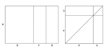
Figure 15: Van der Waerden’s diagrams for II.1 and II.4.

Our Fig. 15 represents van der Waerden’s Figures 33 and 34. They aim to emulate Euclid’s diagrams accompanying propositions II.1 and II.4. Let us notice that these diagrams differ from Euclid’s in regard to the names of line segments – it never happens in the Elements diagrams that different individual lines have got the same name. Moreover, there is no counterpart of line A in Figure 33. It looks like van der Waerden had to modify Euclid’s diagrams to develop his interpretation.

Now, let us take the formula $a(b+c+d)=ab+ac+ad$ designed to correspond to proposition II.1. Which part of the proposition does it formalize: the diorisomos, or the starting point of the proof (the formula in red in our scheme)? In fact, since van der Waerden’s diagram does not represent line A, his account of Euclid’s proof would look like this

$$a(b+c+d)=ab+ac+ad \xrightarrow[]{}$$

$$\vdots$$

$$\xrightarrow[]{} a(b+c+d)=ab+ac+ad.$$

Thus, there is no need for any proof at all.

The same applies to his interpretation of proposition II.4. Instead of

$${\color[rgb]{1,0,0}HF,\,CK,\,AG,\,CE=ADEB} \xrightarrow[]{}$$

$$\vdots$$

$$\xrightarrow[]{} {\color[rgb]{1,0,1}AB^{2}=AC^{2},\,CB^{2},\,2AC\times CB},$$

van der Waerden-style proof would look like this

$$(a+b)^{2}=a^{2}+b^{2}+2ab \xrightarrow[]{}$$

$$\vdots$$

$$\xrightarrow[]{} (a+b)^{2}=a^{2}+b^{2}+2ab.$$

There is also no need for any proof. Indeed, regarding proposition II.4, he writes “The proof can be read off immediately from Fig 34”. However, in the Elements, only the equality in red is read off the diagram, while the final conclusion requires some arguments.

In sum, whatever van der Waerden interprets, these are not Euclid’s propositions.

Finally, we find the following speculations: “We were not able to find any interesting geometrical problem that would give rise to theorems like II 1–4. On the other hand, we found that the explanation of these theorems as arising from algebra worked well” (Waerden 1975, 203). There is no need to dispute whether the distinction between figures represented and not represented on a diagram is a geometrical problem. Whatever it is, it provides an explanation for Euclid’s propositions II.1 to II.4. As regards strictly geometrical problems, II.4 is applied in II.12 which is the ancient counterpart for the cosine rule for obtuse triangle. Below diagram illustrates the use of II.4

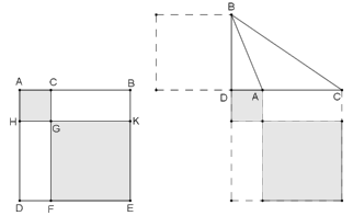
Figure 16: Euclid, Elements, II.4, 12.

Here is the respective scheme.

Diorismos

$$CB^{2}=CA^{2},AB^{2},2CA\times AD.$$

Apodeixis

$$\xrightarrow[II.4]{} DC^{2}=AC^{2},AD^{2},2CA\times AD$$

$$\xrightarrow[]{} DC^{2},DB^{2}=AC^{2},AD^{2},DB^{2},2CA\times AD$$

$$\angle D=\pi/2 \xrightarrow[]{} CD^{2},DB^{2}=CB^{2}$$

$$\xrightarrow[]{} AD^{2},DB^{2}=AB^{2}$$

$$\xrightarrow[]{} CB^{2}=CA^{2},AB^{2},2CA\times AD.$$

The reference to II.4 is easily identified by the way the line CD is cut at the point A: “since the straight-line CD has been cut, at random, at point A, the one on DC is thus equal to the squares on CA, AD, and twice the rectangle contained by CA, AD”. Again, we will not dispute whether the cosine rule is an “interesting geometrical problem”.

In section § 6.1.1, we showed that van der Waerden interprets II.4, 5, 11 as solving specific equations. Significantly, he did not provided similar interpretations for II.12–14.

7.2.2 John T. Baldwin and Andreas Mueller

(Baldwin, Mueller 2019) provides a series of arguments for autonomy of geometry. It includes historical, conceptual and model theoretical ones. As regards history, the paper develops a geometric interpretation of Book II as opposed to van der Waerden’s ‘geometric algebraic’ interpretation, as they call it. Geometry in this context, implicitly, means for them a study of figures represented on the diagrams.

Baldwin and Mueller place Book II within Euclid’s theory of equal figures: “On reflection, there is a natural geometric motivation for the main themes of Book II: Determine a precise method for determining which of two disjoint rectilinear figures (polygons) has the greater area” (Baldwin, Mueller 2019, 8). In fact, only two propositions of Book II, namely II.5 and II.14, complete the theory of equal figures as developed in Book I.

Baldwin and Mueller continue: “Thus, Proposition II.2 certainly implies that if a square is split into two non overlapping rectangles the sum of the areas of the rectangles is the area of the square” (Baldwin, Mueller 2019, 8). However, what they refer to it is the starting point of II.2, not the conclusion. This starting point (the formula in red, in our scheme), as based on visual evidence needs no proof.

Accordingly, they present II.5 as a dissection proof; see (Baldwin, Mueller 2019, 9–10). Here is their proof schematized according to the rules we have already applied to Euclid’s proofs.

By construction, $DB\cong BM$, and $CD\cong MF$. The rest is as follows.

$${\color[rgb]{1,0,0}ADHK=ACLK,CDHL} \xrightarrow[]{}$$

$$ACLK\cong BFGD \xrightarrow[]{}$$

$${\color[rgb]{0,0,1}CB^{2}\ (is)\ (CBFE)} \xrightarrow[]{}$$

$${\color[rgb]{1,0,0}CB^{2}=BFGD,CDHL,LHGE}$$

$$LHGE=CD^{2} \xrightarrow[]{}$$ .

Indeed, Baldwin–Mueller’s proof is a series of observations rather than arguments. It also does not provide a final conclusion. To get it, one should apply the substitution rule, namely ${\color[rgb]{1,0,1}CB^{2}=ADHK,CD^{2}}$.

In the above scheme, equalities in red interpret the phrase “is composed”, the formula $LHGE=CD$ interprets the phrase “LHGE (which has the same area as the square on CD)”. Thus, Baldwin and Mueller provide a styling on Euclidean proof rather than an interpretation of the actual Euclid’s proof.

Historians often point out that algebraic interpretation ignores the role of gnomons in Book II. Baldwin and Mueller managed to turn that objection into a more specific argument, namely: “Much of Book II considers the relation of the areas of various rectangles, squares, and gnomons, depending where one cuts a line. While gnomons have a clear role in decomposing parallelograms, the algebraic representation for the area of gnomon, is not a tool in polynomial algebra. That is, while such equations as $(a+b)(a-b)=a^{2}-b^{2}$ or the formula for product of binomials are tools in algebra which have nice geometric explanation, the area of a gnomon has an algebraic expression, $2ab+a^{2}$, which does not recur in algebra (e.g., as a method of factorization)” (Baldwin, Mueller 2019, 9).

Although Baldwin and Mueller emphasize the role of gnomons, in fact, in their proof of II.5, Euclid’s gnomon NOP is simply a composition of two rectangles: BFGD, CDHL. As a result, they do not provide a counterpart of Euclid’s decisive argument, namely $NOP=AD\times DB$.

What is, then, the role of the gnomon in II.5. Starting from the equality $NOP=AD\times DB$, with προςϰείϑω, Euclid refers to CN2 to get $NOP,LG=AD\times DB,CD^{2}$. What Baldwin and Mueller get by visual evidence, Euclid gets by deduction.

How about Baldwin–Mueller congruence $ACLK\cong BFGD$? By no means it is obvious, as we gave up an algebraic mode. Dissection also seems useless.

Here is how Euclid gets the result $AH=NOP$ in proposition II.5 (see Fig. 11).

$$\xrightarrow[I.43]{} CH=HF$$

$$\xrightarrow[CN2]{} CH,DM=HF,DM$$

$$\xrightarrow[]{} {\color[rgb]{1,0,0}CM=DF}$$

$$AC=CB \xrightarrow[]{} CM=AL$$

$$AL,CH=CM,HF \xrightarrow[]{} {\color[rgb]{1,0,0}AH=NOP}.$$

While Baldwin and Mueller did not manage to represent Euclid’s reliance on gnomons in II.5, contrary to Euclid, they apply gnomon in their proof of II.14.

In II.14, let us remind, it is required to construct a square equal to a rectilinear figure $A$. Within the theory of equal figures, $A$ is turned into a rectangle $BCDE$. And here is where our scheme starts.

$$... \xrightarrow[II.5]{} BE\times EF,GE^{2}=GF^{2}$$

$$GF=GH \xrightarrow[]{} BE\times EF,GE^{2}=GH^{2}$$

$$HE^{2},GE^{2}=GH^{2} \xrightarrow[]{} BE\times EF,GE^{2}=HE^{2},GE^{2}$$

$$\xrightarrow[CN3]{} BE\times EF=HE^{2}$$

$$EF=ED \xrightarrow[]{} {\color[rgb]{.5,0,.5}BD\,\pi\,BE\times EF}$$

$$\xrightarrow[]{} {\color[rgb]{1,0,1}BD=HE^{2}}$$

$$BD=A \xrightarrow[]{} A=EH^{2}.$$

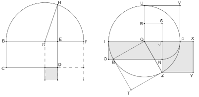
Figure 17: Euclid’s proof of II.14 (left), Baldwin-Meuller version (right).

And here is Baldwin–Meuller proof (see Fig. 17).

$$... \xrightarrow[II.5]{} IJNO,QJ^{2}=QP^{2}$$

$$QP\cong QZ \xrightarrow[]{} {\color[rgb]{1,0,1}QP^{2}=QZ^{2}}$$

$$\xrightarrow[I.47]{} QP^{2}=QJ^{2},JZ^{2}$$

$$\xrightarrow[CN3]{} QP^{2}\setminus QJ^{2}=UVPJR=IJNO=JZ^{2}.$$

The reference to the gnomon $UVPJR$ does not add anything to this proof – from the deductive perspective it is useless. Yet, Baldwin and Mueller created a diagram for II.14 in which every argument (every line in the scheme of their proof) is represented by an individual figure. Yet, they did not manage to find a similar solution for this argument

$$QP\cong QZ\rightarrow QP^{2}=QZ^{2}.$$

Now, let us compare Baldwin–Mueller’s and Euclid’s diagrams. On the one hand, there is a complex composition of rectangles and squares designed to represent every textual argument (Baldwin and Mueller’s arguments, instead of Euclid’s). On the other hand, there is a simple composition which represents, actually, abstract arguments. If we take Euclid’s diagram in its original form (see Fig. 1), we can still recognize how II.5 is applied, and the diagram becomes an ideogram. If there are no other reasons for the use of the terms rectangle contained by and square on, this diagrammatic representation of Euclid’s abstract arguments is the most solid one.

8 Descartes’ lettered diagrams

In this final section, we discuss one of Descartes’ diagrams included in his Geometry. By this contrast, we aim to underline the crucial steps in Euclid’s procedures used in Book II.

In the fragment cited below, Descartes illustrates one of his rules for solving fourth degree equations. The details of his problem are irrelevant for our analysis, therefore they are skipped.

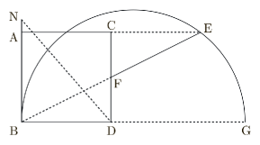
Figure 18: Descartes, Geometry, p. 388.

Here is Descartes’ account of the diagram represented in Fig. 18:

“For, putting $a$ for BD or CD, and $c$ for EF, and $x$ for DF, we have CF $=a-x$, and, as CF or $a-x$ is to FE or $c$, so FD or $x$ is to BF, which as a result gives $\frac{cx}{a-x}$. Now, in the right-angle triangle BDF one side is $x$, another is $a$, then their squares, which are (leures carrés, qui sont) $xx+aa$, are equal to the square of base, which is $\frac{ccxx}{xx-2ax+aa}$” (Descartes 1637/2007, 388/191).

On this diagram, Descartes applies the ancient technique of naming vertices and intersections of lines with capital letters. Nevertheless, when it comes to analysis, he assigns new letters, specifically one letter to different lines: in this case, he puts $a$ for BD and CD. We have already observed that Euclid applies the same trick in proposition II.1. Yet, in the following propositions, he does not explore this idea. As for Descartes, it is his standard procedure. We believe that is where the algebra begins: giving the same name to different objects. The next step in algebraic account of geometry is symbolic computation. As we all know, Descartes developed a technique of symbolic computation. It is the arithmetic of line segments. However, in regard to this initial step, it seems that Descartes does not appreciate it. That is how he explains his technique of naming lines:

“Finally, so that we may be sure to remember the names of these lines, a separate list should always be made as often as names are assigned or changed. For example, we may write, AB=1, that is AB is equal to 1; GH=a; BD = b, and so on. If, then, we wish to solve any problem, we first suppose the solution already effected, and give names to all the lines that seem needful for its construction, to those that are unknown as well as to those that are known. Then, making no distinction between known and unknown lines, we must unravel the difficulty in any way that shows most naturally the relations between these lines, until we find it possible to express a single quantity in two ways. This will constitute an equation, since the terms of one of these two expressions all together equal to the terms of the other” (Descartes 2007, 6–9).

The same letter, x, y or z, can name unknown, and unequal lines. Yet, Descartes does not mention that the same letter can name different, though known and equal lines. It is his practice, not an explicit method. From his perspective, the most important notion is that “a single quantity”, i.e. a line segment, can get two names. In his system, these two names make an equation of two arithmetic terms. However, within the theory of polynomials developed in Book III, these names can be transformed into a polynomial equation $f(x)=0$, and their original meaning, i.e. a reference to a specific line, evaporates.

From our perspective, the crux of Descartes’ method consists in giving one name to different objects: that is the starting point of his equations. However, Euclid has a technique of asserting different names to the same object (renaming, in our terms). The transformations of these names allowed him to relate figures which are represented and not represented on diagrams. The latter only have one name: it can be rectangle contained by or square on. Thus, if one looks for an algebraic prelude in Euclid’s Book II, it could be proposition II.1. Yet, the technique of assigning one name to different objects has not been developed further in the Elements.

References

- [1] Baldwin, J.T., Mueller, A. (2019): The Autonomy of Geometry. Annales Universitatis Paedagogicae Cracoviensis. Studia ad Didacticam Mathematicae Pertinentia 11, 5–24.
- [2] Blåsjö, V. (2016): In defence of geometrical algebra. Archive for History of Exact Science 70, 325–359.
- [3] Błaszczyk, P. (2018): From Euclid’s Elements to the methodology of mathematics. Two ways of viewing mathematical theory. Annales Universitatis Paedagogicae Cracoviensis. Studia ad Didacticam Mathematicae Pertinentia 10, 5–15; https://www.researchgate.net/profile/Piotr_Blaszczyk3/publications
- [4] Błaszczyk, P., Mrówka, K. (2015): Kartezjusz, Geometria. Tłumaczenie i komentarz. Universitas, Kraków.
- [5] Błaszczyk, P., Petiurenko, A. (2019): Euclid’s theory of proportion revised. Annales Universitatis Paedagogicae Cracoviensis. Studia ad Didacticam Mathematicae Pertinentia 11, 37–61; https://www.researchgate.net/profile/Piotr_Blaszczyk3/publications
- [6] Błaszczyk, P., Petiurenko, A. (2020): Modes of diagrammatic reasoning in Euclid’s Elements. In A. Pietarinen, P. Chapman, L. Bosveld de Smet, V. Giardino, J. Corter, S. Linker (eds.) Diagrammatic Representation and Inference - 11th International Conference, Diagrams 2020, Proceedings. Lecture Notes in Artificial Intelligence (LNAI) 12169 Springer.
- [7] Corry, L. (2013): Geometry and arithmetic in the medieval traditions of Euclid’s Elements: a view from Book II. Archive for History of Exact Science 67, 637–705.
- [8] Descartes, R. (1637): La Géométrie. Jan Maire, Lejda.
- [9] Descartes, R. (2007): Geometry of Rene Descartes. Translated from the French and Latin by D.E. Smith and L. M. Lethan. CosimoCLassics, New York.
- [10] Fitzpatrick, R. (2007): Euclid’s Elements of Geometry translated by R. Fiztpatrick; http://farside.ph.utexas.edu/Books/Euclid/Elements.pdf
- [11] Fowler, D. (2003): The Mathematics of Plato’s Academy. Clarendon Press, Oxford.
- [12] Hartshorne, R. (2000): Geometry: Euclid and Beyond. Springer, New York.
- [13] Hilbert, D. (1902); Foundations of Geometry. Authorized translation by E.J. Townsend, Open Court, Chicago.
- [14] Hilbert, D. (1903): Grundlagen der Geometrie. Teubner, Leipzig.
- [15] Mueller, I. (2006): Philosophy of Mathematics and Deductive Structure in Euclid’s Elements. Dover, New York (reprint of the first edition: MIT Press, Cambridge, Massachusetts, 1981).
- [16] Katz, M. (2020). Mathematical Conquerors, Unguru Polarity, and the Task of History. Journal of Humanistic Mathematics 10(1), 475–515.
- [17] Netz, R. (1999): The Shaping of Deduction in Greek Mathematics. Cambridge University Press, Cambridge.
- [18] Oaks, J.A. (2018): François Viète’s revolution in algebra. Archive for History of Exact Science, 72, 245–302.
- [19] Saito, K. (2004): Book II of Euclid’s Elements in the light of the theory of conic sections. Historia Scientiarum 28, 1985: 31–60. Reprinted in Jean Christianidis (ed.). Classics in the History of Greek Mathematics, Kluwer, Dordrecht-Boston, pp. 139–168.
- [20] Van der Waerden, B.L. (1961): Science Awaking. Oxford University Press, New York.
- [21] Van der Waerden, B.L. (1975): Defence of a ‘shocking’ point of view. Archive for the History of Exact Sciences 15(3), 199–210.