Statistics of wide pre-main sequence binaries in the Orion OB1 association

Abstract

Statistics of low-mass pre-main sequence binaries in the Orion OB1 association with separations ranging from 0$\farcs$6 to 20″ (220 to 7400 au at 370 pc) are studied using images from the VISTA Orion mini-survey and astrometry from Gaia. The input sample based on the CVSO catalog contains 1137 stars of K and M spectral types (masses between 0.3 and 0.9 ${\cal M}_{\odot}$), 1021 of which are considered to be association members. There are 135 physical binary companions to these stars with mass ratios above $\sim$0.13. The average companion fraction is 0.09$\pm$0.01 over 1.2 decades in separation, slightly less than, but still consistent with, the field. We found a difference between the Ori OB1a and OB1b groups, the latter being richer in binaries by a factor 1.6$\pm$0.3. No overall dependence of the wide-binary frequency on the observed underlying stellar density is found, although in the Ori OB1a off-cloud population these binaries seem to avoid dense clusters. The multiplicity rates in Ori OB1 and in sparse regions like Taurus differ significantly, hinting that binaries in the field may originate from a mixture of diverse populations.

1. Introduction

Orbital parameters and mass ratios of binary stars depend on their formation environment. It is known that star formation regions (SFRs) of low stellar density, like Taurus-Auriga, spawn a rich binary population, including a substantial number of very wide pairs (Joncour et al., 2017). In contrast, in more dense SFRs the binary fraction is lower, comparable to the field binary population (Duchêne & Kraus, 2013; King et al., 2012). It is generally accepted that most stars in the field were formed in relatively dense environments and that some young wide binaries were destroyed by dynamical interaction with neighboring stars. However, Duchêne et al. (2018) found an excess of close (10–60 au) binaries in the dense Orion Nebula Cluster (ONC), compared to the field. These close binaries are not susceptible to dynamical disruption (Parker & Meyer, 2014). Critical examination of binary statistics in several nearby SFRs has led Duchêne et al. (2018) to the disconcerting conclusion that none of those groups is compatible with the binary statistics in the field. However, the excess of binaries with separations $<$60 au in the ONC has later been contested by De Furio et al. (2019).

The ongoing debate on the origin of the field binary population and the role of SFR density and dynamical interactions in shaping the binary separation distribution stimulates further observational studies. Currently available data on multiplicity statistics suffer from large errors owing to the small size of available samples and from various biases caused by observational constraints or sample selection effects. Modern large–scale surveys and catalogs change the landscape by providing large and homogeneous data sets. For example, the Gaia census of nearby wide binaries gave new insights on the distribution of their separations and mass ratios (El-Badry et al., 2019). A sample of $\sim$600 stars in the Upper Scorpius SFR has been recently observed with high angular resolution to refine the binary statistics (Tokovinin & Briceño, 2020).

Here we use the opportunity to learn about young binaries offered by the combination of three modern surveys: CVSO, VISTA Orion, and Gaia. The CVSO (CIDA Variability Survey of Orion; Briceño et al., 2019) was an optical, multi-epoch imaging survey that produced a large sample of pre-main sequence (PMS) stars across $\rm\sim 180\deg^{2}$ in the Orion OB1 association, spanning all the region between $\alpha_{J2000}=5^{|rmh}-6^{\rm h}$, and $\delta_{J2000}=-6\arcdeg$ to +6° (Figure 1), with an average resolution of 3″ (equivalent to 1112 au at 370 pc) as measured in the original CVSO images. The young stars were selected based on photometric variability and confirmed by follow-up spectroscopy. These PMS stars are mostly located outside the Orion A and B molecular clouds (Maddalena et al., 1986) and we refer to them as off-cloud PMS stars. The off-cloud stars have on average low extinction ($A_{V}\lesssim 0.5$ mag). The spectral types range, mostly, from M5 to K0 and correspond to masses $\sim 0.3-0.9$ ${\cal M}_{\odot}$. The off-cloud CVSO PMS stars are localized in the two main sub-associations in which Ori OB1 was been traditionally subdivided, namely Ori OB1a and Ori OB1b (Blaauw, 1964; Warren & Hesser, 1977), with further sub–clustering within each group (Briceño et al., 2019).

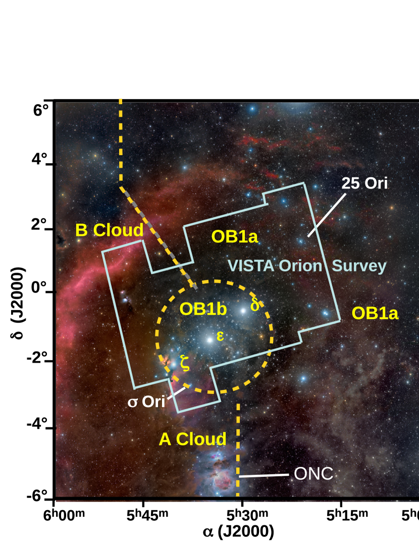
Figure 1.— Wide field optical image of the area encompassed by the CVSO in the Orion OB1 association, showing as an irregular polygon the approximate footprint of the VISTA Orion Survey (Petr-Gotzens et al., 2011). The Orion OB1b sub-association is the region within the dashed line circle, as in Briceño et al. (2005). The OB1a sub-association is the area to the west of the OB1b region and the dashed lines north and south of it, which roughly mark the limits of the Orion A and B molecular clouds, as indicated by the labels. We also indicate the location of the three Orion belt stars $\delta$, $\epsilon$, and $\zeta$ Ori, as well as the $\sigma$ Ori and 25 Ori clusters. The Orion Nebula Cluster (ONC) is also indicated. Photo courtesy of Rogelio Bernal Andreo (http://www.deepskycolors.com/).

The VISTA Orion survey (Petr-Gotzens et al., 2011) covers a 30 square degree area toward the Orion belt and was designed to overlap in large parts with the CVSO footprint, although the total area covered is much smaller, as shown in Figure 1. Its near infra-red (nIR) images in the $Z,Y,J,H,K_{s}$ photometric bands have a typical stellar point spread function FWHM (full width at half maximum) resolution of 0$\farcs$9, and allow us to detect binaries down to 0$\farcs$6 separation (projected separation of $\sim$220 au at 370 pc distance). Statistics of wide binaries can be studied after accounting for chance pairs of unrelated field stars (optical companions). However, distinguishing statistically true binaries from random asterisms becomes progressively uncertain with increasing separation and magnitude difference.

The Gaia Data Release 2 (Gaia collaboration, 2018), hereafter GDR2, contains parallaxes and proper motions (PMs) of most bright stars in the VISTA Orion catalog, allowing a much more reliable distinction between real and optical pairs. At the same time, it helps to clean the main CVSO sample. However, GDR2 has its own problems, mostly caused by close (unresolved) binaries. As a result, reliable GDR2 astrometry is available for most, but not all, stars and companions in Ori OB1. This difficulty can be partially circumvented by using the CVSO and VISTA Orion data. So, all three data sources are more powerful when used jointly.

We define the CVSO-VISTA-Gaia sample of PMS stars in section 2 and discuss its properties such as distance, clustering, etc. Then in section 3 the data on binary stars derived from the combination of the three surveys are presented and characterized. The resulting binary statistics are studied in section 4. We summarize our findings and present our conclusions in section  5.

2. The CVSO-VISTA-Gaia sample of PMS stars

2.1. Target sample selection

The CVSO catalog of young stars in Orion by Briceño et al. (2019) served as a starting point for our target selection. The CVSO contains 2062 spectroscopically confirmed T Tauri stars widely distributed across the Orion OB1 association, mostly in the off-cloud regions, covering well over 100 square degrees on the sky (Figure 1; also, Figure 21 of Briceño et al., 2019). Though not complete, we consider the CVSO to be a representative sample of the population of PMS K and M type dwarfs in the off-cloud regions of the Orion OB1 association, spanning the OB1a and OB1b sub-associations. First, because of how the sample was selected, it is not biased toward accreting stars with optically thick disks, as would be the case of surveys that select objects with strong H$\alpha$ emission or near-IR excesses. Therefore, we expect it to contain a reasonable representation of both accreting and non-accreting PMS stars, most importantly because the later constitute the bulk of the population in the slightly more evolved off-cloud areas of the association. Second, the spatial distribution of the CVSO PMS stars across the OB1a and 1b sub-associations is uniform enough, and there should be no significant, unexpected biases due to sampling only a small area of one or the other region. We point out that because of how it was constructed, the CVSO does not represent the much younger, on-cloud population, which we do not address here.

Positions reported in the CVSO were determined with a custom pipeline that measured an ($x,y$) weighted centroid for each object; these positions were translated to coordinates on the celestial sphere using astrometric transformation matrices referenced to the USNO A-2.0 catalog (Monet, 1998). A positional match between CVSO right ascension and declination coordinates and the 2MASS catalog (Skrutskie et al., 2006), using a $1\arcsec$ radius, yields a Root-Mean-Square (RMS) difference of 0$\farcs$21 $\pm$ 0$\farcs$17, sufficient for matching each source with other catalogs.

We used TOPCAT (Taylor, 2005) to match the CVSO catalog star positions with the VISTA Orion source catalog, that provides accurate positions for $\sim 3\,$ million sources referenced to 2MASS (RMS of $\sim 80$ mas for the residual differential astrometry). The VISTA Orion source positions are an average of the positions determined in each of the photometric bands in which a source was detected. A comparison of the VISTA source positions with the UCAC 4.0 catalog (Zacharias et al., 2013) resulted in an RMS of $\sim 0\farcs 27$ for the absolute astrometry, with no systematic offset (Spezzi et al., 2015). Running a sky match with a $1\arcsec$ search radius between the CVSO and VISTA catalogs yielded 1216 matches, with an RMS of 0$\farcs$22 $\pm$ 0$\farcs$17, which is dominated by the errors in the CVSO positions.

We further restricted the matched sample as follows. We selected all stars that spatially belong to the populations Ori OB1a or OB1b, as shown in Figure 1, but we excluded a 0$\fdg$5 radius around the star $\sigma$ Ori, which is the center of the eponymous stellar cluster. This led to an initial list of 1137 stars, 405 in Ori OB1b, and 732 in Ori OB1a including the 25 Ori and HR 1833 clusters. Table 1 contains all targets, numbered sequentially from 1 to 732 and from 1001 to 1407 for the OB1a and OB1b groups, respectively. These internal numbers $N$, along with the original CVSO numbers, are used throughout the paper.

2.2. Cross-match with Gaia and characteristics of the sample

The next step was to match the sample of 1137 CVSO stars with VISTA catalog information against the Gaia Data Release 2 catalog (GDR2). We first used Vizier to download all stars in GDR2 within a 30″ radius of each of the 1137 CVSO target coordinates. Then, we did a cross-match between this temporary catalog and the CVSO positions, using a 5″ radius and selecting the nearest Gaia source. Coordinate differences between CVSO and Gaia were small for single targets but offsets up to 2″ were found for binaries, because CVSO positions refer to their unresolved (blended) images. When the offsets between the CVSO positions and the actual positions of primary components, determined from the VISTA images as explained below, are accounted for, the rms coordinate difference with Gaia is 0$\farcs$06. Overall, 1078 CVSO stars have GDR2 astrometry. As for the other 59 objects, 55 of them have no parallax and PM information in GDR2, and 4 had no match at all in the GDR2 for no apparent reason (these stars are single and of average brightness: CVSO 685, 1097, 1283, 1819). Finally, we replaced the CVSO equatorial coordinates with the GDR2 coordinates (equinox J2000, epoch J2015.5), which we use from now on.

Having folded in GDR2 astrometry with the CVSO-VISTA sample, we can now take a look at the overall astrometric properties of our target sample. The top panel of Figure 2 shows the location of the 1137 target stars on the sky, where the symbols are colored according to the GDR2 parallax. The 55 stars with no parallaxes or PMs in the GDR2 and the 4 missing stars are marked with crosses. The bottom panel of Figure 2 shows the PM distribution of the 1078 targets having GDR2 astrometry. The closer stars (in red) are more tightly concentrated in PM space, while the more distant population (green and blue) has a larger PM scatter.

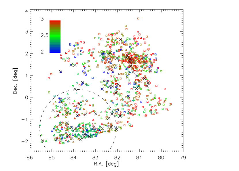
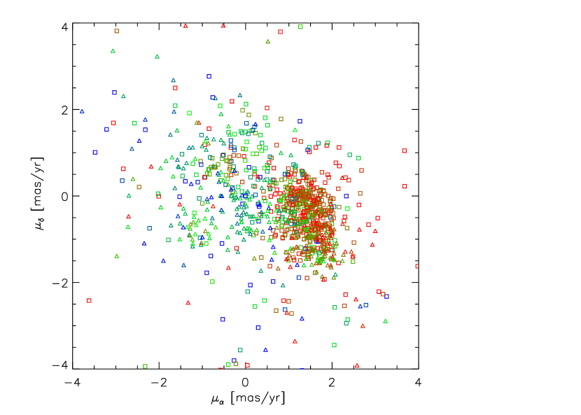
Figure 2.— Top: location of the 1137 CVSO-VISTA objects on the sky (squares for OB1a, triangles for OB1b). The points are colored by parallax in the range from 2 to 3 mas, as shown by the color bar. Black crosses are stars without GDR2 parallaxes. The dashed circle indicates the approximate boundary of the Ori OB1b group. Bottom: distribution of the sample of 1078 objects with GDR2 astrometry in proper motion space. The symbols and colors are the same as in the top panel.

As already noted by Briceño et al. (2019), the GDR2 astrometry shows that Ori OB1 stars are mostly located at distances from 300 to 450 pc, depending on the group. They also show, in accord with Figure 2, that the parallaxes in Ori OB1b have a bi-modal distribution, indicating that closer stars, possibly belonging to Ori OB1a, project on the more distant Ori OB1b group.

The detailed structure of the Orion star-formation region is complex. It has been the subject of several studies using GDR2 astrometry (Zari et al., 2019) and, additionally, radial velocities (Kounkel et al., 2018). Most of our targets belong to the groups C and D identified by Kounkel et al.; these groups have different mean distances (416 and 350 pc, respectively) and radial velocities but spatially overlap on the sky. Since the structure of the Ori OB1 association is outside the scope of this paper, and our focus is on binaries, we use the traditional division into OB1a and OB1b groups based only on the sky location, following the boundaries used by Briceño et al. (2005, 2019). Their mean parallaxes are 2.748 and 2.576 mas respectively, corresponding to distances of 363 and 388 pc. The mean PMs are close to zero and have a dispersion of $\sim$2 mas yr^-1. We point out that groups OB1a and OB1b as considered here are, however, not homogeneous in terms of their age and distance. OB1a contains clusters like 25 Ori and HR1833 within the more widely spread ”field” PMS population. Though it seems clear that OB1a as a whole is a population originating in an earlier star-forming episode compared to OB1b (Kounkel et al., 2018; Briceño et al., 2019), the ages and distances we use are only indicative.

Using GDR2 astrometry, in the next section we will investigate the membership of our targets to Ori OB1a and Ori OB1b, and identify likely non-members. In fact, Briceño et al. (2019) note that their catalog of Orion PMS stars can still be slightly contaminated by active foreground K- and M-type dwarfs with spectral signatures resembling those of PMS stars. For example, CVSO 569 is a 6$\farcs$2 pair of similar stars with almost identical PMs of $(-20,-7)$ mas yr^-1 and parallaxes about 4 mas; this is a physical binary, and its spectrum does show H$\alpha$ in emission and Li I 6707 in absorption, therefore it is clearly a low-mass, PMS star but likely foreground and unrelated to the Orion OB1 PMS population. Finding young stars with motions discrepant from those generally agreed to characterize the bona-fide Orion OB1 population seems increasingly less surprising, since recent studies find that the structure of the stellar population across Orion is richer and more complex than previously thought (Chen et al., 2019; Kos et al., 2019).

2.3. Analysis of the GDR2 astrometry

The large distance to Ori OB1 and its small PM mean that very accurate astrometry is needed to discriminate true association members from foreground and background stars. In addition, unresolved binaries degrade the quality of GDR2 astrometry. Therefore, we focus in the following on filtering out from our targets the likely non-members, but keep those that potentially have their Gaia astrometry compromised due to the presence of a binary companion. The latter can be evidenced in three different ways.

First, pairs with separations from 0$\farcs$1 to 0$\farcs$7 and moderate magnitude difference $\Delta m$ often have undetermined astrometric parameters (parallax and PM) because they were recognized as non-point sources. For example, all GDR2 stars without parallaxes were resolved in the speckle interferometric survey of Upper Scorpius (Tokovinin & Briceño, 2020). There are 55 of our targets that do not have GDR2 parallaxes (section 2.2). Second, the GDR2 astrometry of many close binaries, when present, is often substantially biased because their motion does not conform to the standard 5-parameter astrometric model. Typically, these stars have large errors of astrometric parameters, e.g. the parallax error $\sigma_{\varpi}$. Our experience shows that the parameters of such stars can deviate from their true values (known, e.g., from wide components of well-resolved physical triple systems) much larger than allowed even by those inflated errors. In short, the GDR2 astrometry of these stars is unreliable. Third, even when the 5-parameter astrometric model is adequate, the PM can still be slightly biased by the orbital motion in a long-period binary. A solar-mass binary with a semimajor axis $a$ (in au) and a typical mass ratio of 0.5 would have the orbital PM on the order of $1.8(10/a)^{0.5}$ mas yr^-1 at a distance of 370 pc.

Figure 3.— Parallax errors vs. $G$ magnitude (crosses). The full line is $\sigma_{0}(G)$ defined by equation. 1, the dashed line represents $2\sigma_{0}(G)$.

In order to define a measure for the reliability of GDR2 astrometry specific to our target sample, we plot in Figure 3 the parallax error vs. $G$ magnitude for all targets with GDR2 astrometry and having $G<19$. Note, for very faint targets the GDR2 astrometry becomes very uncertain and we therefore reject a priori 17 stars with $G>19$, which means in the context of our analysis we define those as non-members. The distribution shown in Figure 3 follows a well-defined trend which we approximate by the formula

$$\sigma_{0}(G)\approx 0.024+0.017(G-13)+[0.025(G-16)^{2}],$$ (1)

where the quadratic term is added only for $G>16$ and $\sigma_{0}(G)$ is in mas. We then use the ratio of the parallax error to its model, $r_{\varpi}=\sigma_{\varpi}/\sigma_{0}(G)$, as a measure of the excess astrometric noise indicative of biased GDR2 astrometry. The Gaia errors depend on the source position on the sky, and we caution against using our simplistic model (1) in a more general context; it is just suitable for Orion.

Figure 4 plots the parallax and total PM of our targets with colors that correspond to $r_{\varpi}$. Targets with reliable astrometry, defined here as $r_{\varpi}<2$, are tightly concentrated at parallaxes between 2.2 and 3.2 mas and PMs below 3 mas yr^-1. A bi-modal distribution of parallaxes can be noted. Considering potential biases caused by unresolved binaries, we adopt the following relaxed criteria. Targets with $G<19$ and parallaxes from 1.5 to 4 mas and a total PM less than 5 mas yr^-1, irrespective of their excess noise $r_{\varpi}$, are considered astrometrically confirmed members of Ori OB1. There are 934 stars that comply with these criteria and are assigned a membership flag 2 in Table 1. The high rate of astrometrically confirmed members of Ori OB1 validates the spectroscopic and photometric selection of young stars adopted in the construction of the CVSO sample. For comparison, Kounkel et al. (2018) adopted a parallax range from 2 to 5 mas and the PM limit of $\pm$4 mas yr^-1 in both coordinates as membership criteria.

All targets with reliable astrometry, i.e. $r_{\varpi}<2$, but total PM and parallax values outside our adopted selection box are considered astrometric non-members (membership flag 0 in Table 1, 89 stars). The remaining 41 stars with unreliable GDR2 astrometry (likely close binaries) outside the adopted parallax and PM limits (including three with negative parallaxes) are considered as members, unless their total PM is larger than 13 mas yr^-1. This PM threshold is chosen by examining the tail of the PM distribution and applies to only 6 stars, which means 35 stars are finally considered as members. These members are assigned the membership flag 1 to distinguish them from astrometrically confirmed members. Membership flag 1 is also assigned to 52 stars with missing GDR2 astrometry and $G<19$. Admittedly, the threshold $r_{\varpi}<2$ used here to define reliable astrometry is arbitrary; a smaller threshold of 1.5 increases the number of targets with questionable astrometry by 56, but combination of all membership criteria leads to the same sample size of 1021.

The four stars not found in GDR2, the 17 stars fainter than $G=19$ mag, and the 6 stars with unreliable GDR2 astrometry and total PM larger than 13 mas yr^-1 are excluded from the following statistical analysis together with the astrometrically confirmed non-members (membership flag 0). The numbers of targets with various membership status are reported in Table 2. Overall, there are 1021 members, 658 in Ori OB1a and 363 in Ori OB1b. We provide data for all 1137 targets of the original sample and their companions and use the membership flag defined here only for evaluation of the multiplicity statistics.

The CVSO-VISTA-Gaia targets are listed in Table 1. They are numbered sequentially from 1 to 732 for stars in Ori OB1a and from 1001 to 1407 for those in Ori OB1b (the latter group contains 405 stars). Within each group, the targets are ordered in the right ascension. These numbers $N$, along with the CVSO numbers from Briceño et al. (2019), link the targets to the lists of double stars presented below. In the following columns of Table 1 we give the information extracted from GDR2, namely the equatorial coordinates (equinox J2000, epoch 2015.5), parallax $\varpi$, its error, proper motions $\mu^{*}_{\alpha}$ and $\mu_{\delta}$, and the $G$ band magnitude. The $J$ magnitude from 2MASS and the spectral type are retrieved from the CVSO catalog. The last three columns contain the excess noise $r_{\varpi}$ (zero if parallax is not known), the membership flag, and, for binaries, the separation in arcseconds.

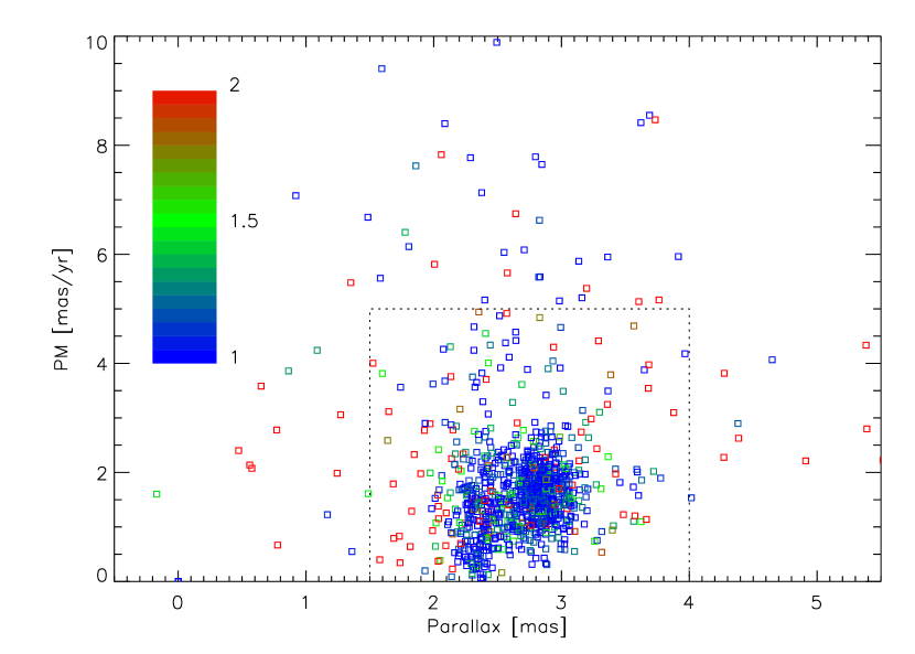
Figure 4.— Correlation between parallax and total PM for our sample. The symbols are colored according to the excess error $r_{\varpi}$, as shown by the color bar. The dotted box shows the limits of parallax and PM adopted for the 934 astrometric members.

Table 1CVSO-VISTA-Gaia sample (fragment)

$N$	CVSO	$\alpha_{2000}$	$\delta_{2000}$	$\varpi$	$\sigma_{\varpi}$	$\mu^{*}_{\alpha}$	$\mu_{\delta}$	$G$	$J$	Spectral	$r_{\varpi}$	Memb.	$\rho$
		(deg)	(deg)	(mas)	(mas)	(mas yr-1)		(mag)	(mag)	type			(″)
1	405	79.57240	$-$0.32216	3.41	0.37	0.98	$-$0.28	18.56	14.99	M4.5	1.30	2	0.00
2	408	79.60478	$-$0.33421	2.73	0.27	1.14	0.38	18.56	15.02	M3.0	0.96	2	0.00
3	416	79.68400	$-$0.56678	2.86	0.03	10.50	17.79	14.73	12.59	M0.0	0.51	0	0.00
4	425	79.76144	$-$0.54096	3.00	0.08	1.73	$-$1.02	16.07	13.11	M3.0	1.04	2	0.00
5	427	79.78025	$-$0.09696	2.55	0.17	1.52	$-$0.89	17.62	14.41	M3.0	1.01	2	0.00
6	432	79.82293	$-$0.18850	2.78	0.08	2.00	$-$0.82	16.51	13.49	M4.0	0.86	2	3.44

Table 2Classification of the targets

Member flag	$N$	$0<r_{\varpi}<2$	$r_{\varpi}>2$	$r_{\varpi}=0$
2	934	869	65	0
1	87	0	35	52
0	116	102	7	7

2.4. Photometry and CMD

Figure 5.— Cumulative distributions of $J$ magnitudes for all targets classified as members (flag 1 or 2).

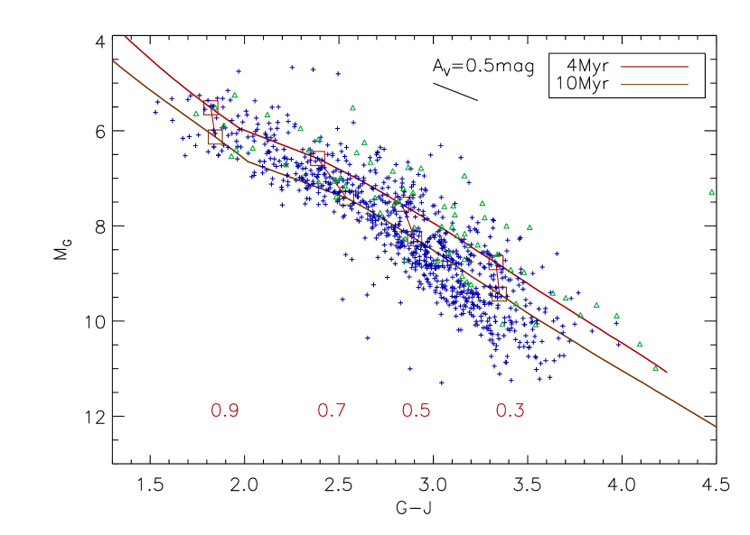
Figure 6.— Color-magnitude diagram. Known binaries with separations less than 5″ are plotted by green triangles, other stars by blue crosses. Absolute magnitudes have been derived for each star based on its parallax. Two PARSEC isochrones for solar metallicity are plotted. The squares on the isochrones and numbers mark masses from 0.3 to 0.9 ${\cal M}_{\odot}$. The line marks the effect of an $A_{V}=0.5$ mag extinction.

Figure 5 shows cumulative distributions of $J$ magnitudes for members of Ori OB1a and Ori OB1b. The medians are 13.21 and 12.93 mag, respectively, consistent with Ori OB1a being slightly older than Ori OB1b; the median $G$ magnitudes in these groups are 16.20 and 15.89 mag.

The color-absolute magnitude diagram (CMD) in Figure 6 shows only 934 astrometrically confirmed members of the association with measured parallaxes. We plot the 4 Myr and 10 Myr PARSEC isochrones for solar metallicity (Tang et al., 2014) using the 2MASS and Gaia colors and mark corresponding masses; these ages are consistent with those adopted by Briceño et al. (2019) for OB1b (5 Myr) and OB1a ($\sim 11$ Myr); remember though that these groups are not strictly coeval, as noted before. We do not use here the VISTA Orion photometry because for brighter targets it is biased by saturation. The extinction is not corrected for, but since these are off-cloud populations, the overall reddening is small. In fact, for our sample the median extinction $A_{V}$ determined in the CVSO catalog (Briceño et al., 2019) is 0.36 mag. About 24% targets have $A_{V}=0$, and only 11% have $A_{V}>1$ mag. According to Danielsky et al. (2018), $A_{V}=1$ mag corresponds to $A_{G}=0.47$ mag and $A_{J}=0.24$ mag for a star of 4000 K effective temperature. The $A_{V}=0.5$ mag vector plotted in Figure 5 displaces stars almost parallel to the isochrones. The low-mass stars appear to be bluer (or fainter) compared to the isochrones, showing that evolutionary models of PMS stars are still far from perfect. This systematic deviation from the isochrones is confirmed by our photometry of binaries, see section 3.5.

Binary stars are located on the CMD above the single-star isochrone. Known binaries with separations less than 5″ are distinguished in Figure 6 by green triangles. The $G$ magnitudes of those 61 targets refer to the primary components resolved by Gaia, while their $J$ magnitudes from 2MASS refer to the combined light, displacing the points to the right by as much as 0.75 mag. However, the majority of binaries are not recognized because they are closer than 0$\farcs$6, the resolution limit of our survey. Binarity certainly contributes to the scatter in the CMD.

The CMDs of various sub-groups of the Ori OB1 associations are plotted and discussed by Briceño et al. (2019) and Kounkel et al. (2018). They derive model-dependent ages ranging from 4 to 13 Myr for various sub-groups. However, even within one sub-group the spread of the CMD is substantial. One of the reasons is that all CVSO stars are variable (this was one of the selection criteria in building the sample). The variability of low-mass PMS stars ranges from a median value of 0.5 mag in the $V$ band for accreting Classical T Tauri stars, caused by a combination of variable accretion, rotational modulation by hot/cold spots and possible disk obscuration, down to $\sim 0.3$ mag for the non-accreting Weak-lined T Tauri stars, in which variability is mainly due to rotational modulation by dark spots and chromospheric activity (Briceño et al., 2019). The photometry provided in the CVSO catalog is averaged over time, reducing the impact of variability. But the 2MASS and Gaia photometry are not simultaneous, and they are mostly single-epoch measurements, therefore variability contributes to the errors of colors and increases the scatter in the CMD.

Figure 6 implies that most CVSO stars have masses between 0.3 and 0.9 ${\cal M}_{\odot}$, with 0.4 to 0.8 ${\cal M}_{\odot}$ being dominant, i.e., spectral types $\sim$K2 to M4 (see Figure 1 in Briceño et al., 2019). However, masses of PMS stars estimated from absolute magnitudes or colors are known to be highly uncertain. The isochrones appear to deviate systematically from the observed pre-main sequence, and the problem is aggravated by the intrinsic variability of all CVSO stars that adds uncertainty of magnitudes and colors. Moreover, ages for individual stars are not well determined and there appears to be a considerable age spread in both sub-associations. Given these intrinsic uncertainties, we refrain here from estimating individual masses and mass ratios. A crude estimate of mass ratios based on the isochrones is used here only for the purpose of translating the limit of our survey from photometric contrast into approximate mass ratio. The isochrones suggest that the magnitude difference in the $J$ band is related to the mass ratio of a young binary $q=M_{2}/M_{1}$ as $q\approx 10^{-0.3\Delta J}$ (see section 4.1). In the following, we estimate approximate mass ratios using this formula without insisting on its correctness or uniqueness. According to this relation, binaries with $\Delta J<3(2)$ mag have $q>0.13(0.25)$. Therefore, by restricting our statistical analysis to pairs with $\Delta J<3$ mag, we cover most of the mass ratio range, while rejecting fainter (and mostly unrelated) companions.

2.5. Clustering and chance projections

Figure 7.— Surface density of companions vs. separation in Ori OB1a and OB1b. The dotted line shows the companion density in Taurus according to Larson (1995).

Companions belonging to the Ori OB1 group according to the astrometric and photometric criteria are not necessarily bound to the main targets. Instead, they could be random pairs of association members projecting close to each other on the sky. To elucidate this issue, we computed the spatial density of CVSO stars around each target in 4 annular zones with a logarithmic radius step of 0.5 dex, from 9″ to 900″ (0$\fdg$25). The two subgroups OB1a and OB1b are treated separately. The surface density of association members in annular zones around our targets is plotted in Figure 7, assuming a common distance of 370 pc. The average density in both groups is similar, about 55 stars per square degree.

The dotted line in Figure 7 depicts the companion density in Taurus which, according to Larson (1995), is well approximated by a broken power law with the exponents of $-0.62$ at separations exceeding $10^{4}$ au and $-2.15$ at closer separations. Compared to Orion OB1, Taurus has a much lower density and a stronger clustering inherited from the structure of molecular clouds. In contrast, in the older Orion OB1 association the stars are well mixed at scales less than a parsec, although they retain clustering at larger scales (Briceño et al., 2019, see also Figure 2).

The first bin shows a reduced stellar density in Ori OB1a compared to larger scales, in strong contrast with Taurus. Taken at face value, this implies an anti-correlation, i.e. avoidance of close pairs relative to a uniform distribution. Most likely, this is a selection effect that arises from the construction of the CVSO sample. It used multi-fiber spectroscopy for confirming the PMS nature of $\sim 70$% of the candidates. Because there is a minimum distance on the sky between adjacent fibers (e.g. $20\arcsec$ for Hectospec; Fabricant et al., 2005), close companions (also PMS stars) would not have been observed for this technical reason. Therefore, we ignore this effect and assume that the average density is 55 stars per square degree in both groups. This means that we expect to find 1.4 and 5.4 random pairs of association members within 10″ and 20″, respectively, in a sample of 1021 stars. However, this is only a lower limit because the CVSO does not contain a complete census of the association members; this is further explored below using GDR2. The expected number of random pairs is subtracted in the following analysis of the separation distribution. We restrict the statistical analysis to separations below 20″ and to moderate $\Delta m$ to minimize the impact of random pairs. Extending these limits would aggravate the uncertainty caused by random pairs of association members.

3. Observational data and their analysis

Our primary source of data on binaries is the examination of the images from the VISTA Orion mini-survey. We attempted to detect almost all companions within 7″ from all original 1137 CVSO stars visible in the images and only later realized that the detection depth is excessive for our survey that needs only a contrast up to 3 mag. When studying the binary frequencies (section 4) we will restrict the analysis to the members of Ori OB1. We complemented the image analysis by searching for wider pairs in the VISTA Orion photometric catalog and by identifying all pairs in the GDR2. Joint analysis of this information allows us to discriminate real binaries from unrelated (optical) asterisms and sets the stage for the statistical analysis presented in section 4.

3.1. Detecting binaries in the VISTA images

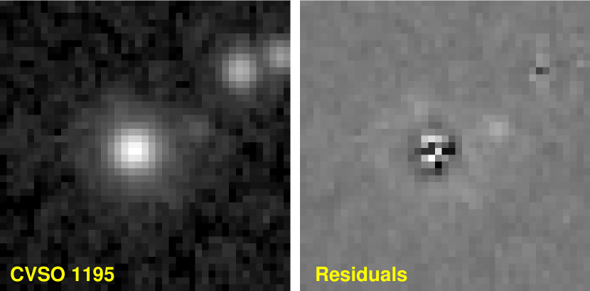
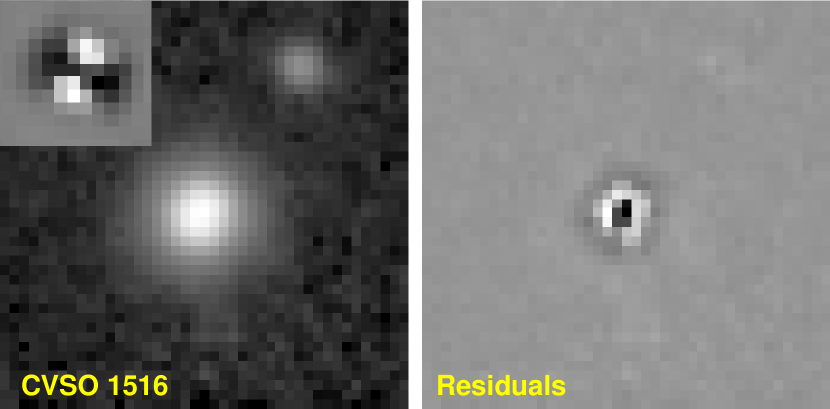
Figure 8.— Modeling the postage-stamp images by Moffat functions. The images are shown on the left, the residuals on the right. Top: the image of target 1027 (CVSO 1195) in the $H$ band with three stars. Note another faint star in-between that has been ignored. Bottom: the image of target 1176 (CVSO 1516) in the $J$ band, with an insert showing residuals for the main star indicating the elongation. The residuals after fitting three stars (on the right) are smaller.

The VISTA Orion mini-Survey (Petr-Gotzens et al., 2011) provides seeing-limited images with a typical FWHM resolution of 0$\farcs$9 (details are given at the end of this section). Data were acquired with VIRCAM, the VISTA nIR wide-field imaging camera that has an average pixel scale of 0$\farcs$341/pix. Observations at $Z,Y,J,H,K_{s}$ bands for one field were executed sequentially in all filters, spanning no more than 2–3 hours in total. This way effects of variability on the stars’ colors should have been diminished.

For each CVSO target, fragments of VISTA images of 43$\times$43 pixels, corresponding to a size of 14$\farcs$7$\times$14$\farcs$7, centered on the nominal target position reported in the CVSO catalog were selected. They are called “postage stamps” or “stamps”. Companions with separations up to 7″ (up to 10″ in the corners) can be found in these postage stamps. The VISTA/VIRCAM focal plane is a mosaic of detectors, with large gaps in between, that must be dithered in a 6-point pattern to contiguously fill the field of view. Furthermore, at $Z$ and $Y$ filters long and short exposures were taken. This means targets were imaged several times in all five filters. However, images where targets fall near a detector edge are partially truncated. Among the 37,464 postage stamps used in this project, 836 severely truncated ones are ignored. On average, there are 5 images per target in the filters $Z$ and $Y$, 10 images in $J$ and $H$, and only 2.4 in $K_{s}$; some targets lack the $K_{s}$–band images altogether.

We used a custom IDL code to process these images, automating the work as much as possible. For each target, the program selects all postage stamps and displays the chosen (usually the first) image in a graphical window. The user defines the number of visible stars and their approximate positions and fits a model to determine accurate relative positions and intensities of these stars. Modeling of all other images of this same target can then be done by one command, using previous results as a first approximation.

Several important comments are in order here. First, all CVSO targets are 4 to 6 mag brighter than the faint magnitude limit of the VSTA Orion survey, assuring that well-resolved companions with a contrast under 3 mag are always securely above the noise-limited detection threshold. Second, no good estimates of the point spread function (PSF) are available because many postage stamps contain just one star, the target itself. So, a decision on whether the PSF asymmetry is caused by a close semi-resolved companion or by a residual telescope jitter (the ellipticity of most images reported in the headers is under 0.05, but in some cases reaches 0.1) is not always straightforward. Unlike the situation in the survey of De Furio et al. (2019), where accurate models of both PSF and noise were available, detections of close companions in the VISTA images cannot be automated and their significance cannot be rigorously evaluated by a metric like $\chi^{2}$. On the positive side, however, we have multiple images of each target obtained under different seeing conditions in five filters. Therefore, the companions are confirmed as many times as there are images. Mutual agreement of binary-star parameters derived from many independent postage-stamp images guarantees the reliability of detections; they are all secure and there are no false positives, as indicated by the independent detection of all, except one, VISTA close binaries (0$\farcs$6 $<\rho<$ 1$\farcs$2) by GAIA and/or high spatial resolution observations (cf. section 3.7). The detection limit is further discussed in section 3.4.

The background level in each image is determined by the median pixel value and further refined by excluding pixels around known stars within a radius of four times the FWHM resolution, typically about 12 pixels. Images of stars that do not overlap significantly can be modeled by fitting a symmetric Moffat profile

$$F(x,y)=\frac{p_{2}}{[1+r^{2}/a^{2}]^{\beta}},\;\;r^{2}=(x-p_{0})^{2}+(y-p_{1})^{2}$$ (2)

with five free parameters $p_{0},p_{1},p_{2},p_{3}=a,p_{4}=\beta$. The first two parameters are pixel coordinates of the center, the third is the maximum intensity, the parameters $a$ and $\beta$ define the width and shape of the point spread function (PSF). The FWHM equals $2a\sqrt{2^{1/\beta}-1}$. The background level is subtracted prior to fitting and not included in the model. The PSF is fitted by minimizing $R$, the un-weighted normalized rms difference between the image $I_{i}$ and its model $M_{i}$ over all pixels $i$ within a radius of 10 from the center:

$$R=\sqrt{\sum_{i}(I_{i}-M_{i})^{2}}/\sqrt{\sum_{i}I_{i}^{2}}.$$ (3)

The residuals for single stars are dominated by the difference between the actual PSF shape and its model (2), rather than by the detector and photon noise. Hence $R$ is the appropriate goodness of fit metric and its minimization achieves the best approximation of the PSF shape. For modeling saturated stars, pixels near the center can be excluded. We also tested elliptical Moffat models with two additional parameters, ellipticity and orientation, but found that the symmetric model (2) works well in most cases; therefore, the elliptical Moffat function was not used.

When the pair is well separated, we model the secondary star by fixing the PSF parameters to those of the primary and fit only the position and relative intensity. For partially overlapping stars, we have the option of adjusting the common parameters $a$ and $\beta$ for all stars, i.e. $2+3n$ parameters for an image containing $n$ stars. This method works very well even for close (blended) pairs and it was used for measuring all companions. Residuals after fitting a triple source 1027 (CVSO 1195) are shown in Figure 8. The two companions are separated from the main star by 6$\farcs$7 and 8$\farcs$7 and have $\Delta J$ of 2.3 and 2.9 mag, respectively; both are unrelated field stars.

Detection of close binaries with separation less than the FWHM is helped by modeling the PSF by a symmetric Moffat function and visual examination of the residuals. A persistent asymmetry of multiple images of the same target indicates a real companion, as opposed to occasional PSF elongation. An a posteriori test of companion detection is furnished by comparison with Gaia (section 3.3). The lower panel of Figure 8 illustrates modeling of the close binary star 1176 (CVSO 1516) in an image with a FWHM resolution of 0$\farcs$96. The residuals after approximating the central star by a symmetric Moffat function (in the insert) have a “butterfly” shape indicative of asymmetry and are large, $R=0.156$. Modeling the central star by two point sources separated by 0$\farcs$61 yields smaller residuals of $R=0.056$. This pair and the 0$\farcs$75 pair # 697 (CVSO 1567) were overlooked initially in the VISTA images but found in Gaia and re-fitted. All other overlooked Gaia pairs are closer than 0$\farcs$6.

Table 3Companions found in the images (fragment)

$N$	CVSO	$\theta$	$\rho$	$\sigma_{\rho}$	$\Delta Z$	$\Delta Y$	$\Delta J$	$\Delta H$	$\Delta K_{s}$	$\sigma_{\Delta Z}$	$\sigma_{\Delta Y}$	$\sigma_{\Delta J}$	$\sigma_{\Delta H}$	$\sigma_{\Delta Ks}$
		(degr)	(″)	(″)	(mag)	(mag)	(mag)	(mag)	(mag)	(mag)	(mag)	(mag)	(mag)	(mag)
1	405	340.1	3.653	0.201	5.61	5.59	5.06	4.89	…	0.19	0.35	0.16	0.00	…
4	425	154.6	3.457	0.019	5.06	5.12	5.24	5.23	4.93	0.15	0.24	0.00	0.00	0.00
5	427	12.1	7.249	0.026	2.64	3.23	3.57	3.88	3.76	0.02	0.16	0.16	0.30	0.08
6	432	101.9	3.440	0.019	2.15	1.91	1.76	1.89	1.76	0.03	0.04	0.00	0.04	0.01
14	455	228.5	7.596	0.147	5.58	5.59	5.73	5.70	…	0.19	0.31	0.00	0.00	…
19	461	40.5	7.402	0.041	4.62	4.64	4.14	3.94	3.16	0.13	0.24	0.15	0.07	0.07

Although our statistical analysis considers only companions with a contrast up to 3 mag, for the sake of completeness we report in Table 3 all companions with $\Delta m<7$ mag found in the postage stamp images. Its first two columns give the sequential and CVSO numbers matching those in Table 1. The position angle $\theta$ and separation $\rho$ are average values for all processed images in all filters where the given companion is detected. The rms scatter $\sigma_{\rho}$ gives an idea of the internal agreement between these measurements. The following five columns give the average magnitude differences in the VISTA $Z,Y,J,H,K_{s}$ bands. The remaining five columns contain the rms scatter of $\Delta m$ in each filter where two or more measurements are available. For a single measurement, the scatter is zero. Some companions lack measurements in some filters either because these images are unavailable or because the companions were not detected owing to noise or truncation. Table 3 contains 490 rows, i.e. unique companions to our 1137 targets, with all companions having a detection in at least two filters. The majority of targets have one companion, and at most four. Most of these companions are unrelated field stars.

The Moffat models also provide the FWHM resolution in each image through parameters $a$ and $\beta$. Its median value is 0$\farcs$88, the mean is 0$\farcs$89, and the dispersion is 0$\farcs$20. Ninety per cent of FWHM values are comprised between 0$\farcs$74 and 1$\farcs$12.

3.2. Wide pairs in the VISTA Orion photometric catalog

The VISTA Orion photometric catalog contains equatorial coordinates and $Z,Y,J,H,K_{s}$ magnitudes of all point sources found in the survey. The catalog is typically complete (at $10\sigma$ significance) to $Z=21.7$, $J=19.6$, and $K_{s}=17.9$ mag, as inferred from the histograms of the magnitudes. This ensures that the companion search in the catalog is sensitive to all companions with $\Delta J<3$ mag, as the faintest target has $J\sim 16$ mag.

The catalog was also used to study the stellar density as a function of magnitude in the area of the Ori OB1 association, to account statistically for the background contamination. The number of stars $n$ per square degree brighter than a certain $J$ magnitude is $\log_{10}n(J)\approx 3.44+0.24(J-15)$ in both groups of Ori OB1. These models are no longer needed in the light of Gaia, but could be used to compute the density of unrelated companions.

We retrieved as companions all catalog stars that are separated between $2\arcsec-20\arcsec$ from the CVSO target position and have $\Delta J<3$ mag. Separations and position angles of these wide pairs are deduced from the equatorial coordinates. We compared the results of our postage-stamp processing with the VISTA Orion catalog for pairs wider than $\sim$2″. The comparison revealed that coordinates of single stars in the CVSO catalog match their VISTA Orion coordinates with a median offset of only 0$\farcs$047 and the maximum offset of 0$\farcs$23. However, for binaries the spatial match was much worse because the CVSO positions refer to the centroids of blended images owing to its 3″ typical FWHM resolution. Our image analysis gives the offsets of the main component from the postage-stamp center (which is at the CVSO position). The CVSO coordinates corrected for these offsets match the VISTA positions with a median difference of 0$\farcs$05. The improved target coordinates also help to match the main stars to the GDR2 without ambiguity. Overall, we found a very good agreement between the relative astrometry and photometry of common pairs produced by our image modeling with those derived from the VISTA Orion catalog, although there are a few outliers. Companions wider than 7″ are found in the VISTA Orion catalog, without the need to examine the images. We added 411 wide pairs with $\Delta J<3$ mag and separation 7″$<\rho<20\arcsec$ to the companion list, thus extending the separation range to 20″. The majority of these wide companions are unrelated field stars, as shown below in section 3.5.

3.3. Companions in GDR2

Figure 9.— Separation versus $\Delta G$ of companions found in Gaia within 20″. The line shows the detection limit $\Delta G<5(\rho-0.5)^{0.4}$ that approximates the detection limit at 50% probability found by Brandeker & Cataldi (2019).

The GDR2 catalog was queried within 30″ radius of each target. The coordinate offsets determined from the image analysis helped to match securely the main targets with GDR2 (the coordinates agree within $\sim$0$\farcs$06).

Most stars found in GDR2 around each target are unrelated (optical) companions. Their separations and $\Delta G$ are plotted in Figure 9. We matched the VISTA Orion pairs to the list of companions in GDR2 and thus retrieved the GDR2 astrometry and photometry for all pairs, except for four close ones with separations below $\sim$0$\farcs$7 (targets No. 392, 597, 1071, 1270) not resolved by Gaia (possibly their secondary components were too faint in the $G$ band). Conversely, six close pairs in GDR2 were not recognized in the VISTA images (targets No. 253, 458, 697, 1176 1257, 1258). All except two have separations below 0$\farcs$6. Sources 697 (0$\farcs$75) and 1176 (0$\farcs$61) were overlooked in the original analysis of the VISTA images and added later (see Figure 8). All other companions found in GDR2 with separations $>$0$\farcs$6 were also detected in the VISTA images or in the survey catalog.

The membership in the Ori OB1 association was tested for each companion candidate with reliable astrometry (measured parallax and PM and $r_{\varpi}<2$). If its parallax and PM satisfy the membership criteria adopted here (Figure 4), the pair is considered real (physical) and its flag is set to $p_{\rm astro}=1$. Otherwise, $p_{\rm astro}=0$ and the pair is considered optical. For 78 companions with missing or unreliable astrometry, we set $p_{\rm astro}=0.5$ and use other criteria to test their membership (see section 3.5). The rms PM difference between the primary and secondary components of 40 physical pairs with $p_{\rm astro}=1$, $\rho<5\arcsec$, and reliable GDR2 data for both components is 0.6 mas yr^-1. We suspect that unrecognized inner subsystems contribute to the scatter of relative motions in these wide pairs.

Figure 10.— Comparison of double-star astrometry between VISTA Orion and Gaia. Squares are astrometrically confirmed association members, pluses are other (mostly optical) companions with $\Delta G<3$ mag. The top plot compares separations, the lower plot shows the tangential difference $\rho\sin\Delta\theta$. The axis scale is in arcseconds.

We compared the relative astrometry derived from the VISTA images with the presumably more accurate GDR2 astrometry (Figure 10). The agreement is excellent for astrometrically confirmed members with $p_{\rm astro}=1$ and $\rho<7^{\prime\prime}$, measured by us in the images. The mean offsets between the relative companion’s positions in the VISTA images and in Gaia in the radial and tangential directions are +1 and +2 mas, respectively, while the rms scatter of these offsets is 8 mas in both directions. On the other hand, the positions of pairs wider than 7″ rely on the coordinates from the VISTA Orion catalog and are accurate only to a fraction of an arcsecond.

3.4. Detection limit

Figure 11.— Location of companions in the $(\rho,\Delta J)$ plane. Squares denote pairs found in our image analysis, crosses plot companions found both in the images and in the VISTA Orion catalog. The dashed line is the empirical detection limit (eq. 4), the dotted rectangle marks the limits of our statistical analysis.

Figure 11 plots the location of all companions in the $(\rho,\Delta J)$ plane. One can appreciate the advantage of our image analysis in terms of resolution and contrast, compared to using solely the VISTA Orion catalog.

The companion detection in the VISTA images depends on the variable FWHM resolution and on the signal to noise ratio. Here we use the simplified optimistic empirical detection limit (dashed line in Figure 11) described by the formula

$$\Delta J<6(\log\rho+0.25)^{0.5},\;\;\;\rho>0\farcs 6.$$ (4)

This formula is chosen “by eye” to fit the envelope of the points. We also studied the empirical detection threshold as a function of FWHM resolution, but, considering the limited range of FWHM variation and multiple images available for each target, decided on a simpler alternative (4). According to this formula, all pairs with separation $\rho>1\farcs 2$ and $\Delta J<3$ mag are detected in the images. In the following, we restrict the statistical analysis to pairs with $\Delta J<3$ mag and ignore fainter companions, making their detection limit irrelevant to our study. Only the contrast and resolution limit at small separations is relevant.

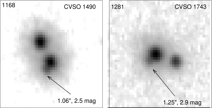
Figure 12.— Postage-stamp $H$-band images of two triple systems with close faint companions, in negative rendering. Separations and $\Delta J$ of close inner pairs are indicated. Left: target 1168 (CVSO 1490), FWHM resolution 0$\farcs$73. Right: target 1281 (CVSO 1743), FWHM resolution 0$\farcs$87.

As noted above, all our detections with $\rho>0\farcs 6$ are secure (no false positives). However, visual detection of close companions by examination of residuals after subtracting the Moffat profile is subjective. Comparison with Gaia reveals that two close pairs were actually missed by our subjective procedure; they were recovered later by modeling images as a double, rather than single, source. Conversely, four similarly close pairs were unresolved by Gaia. The mean $\Delta J$ of physical companions in the 0$\farcs$6-1$\farcs$2 and 1$\farcs$2-2$\farcs$4 separation bins are 0.86 and 0.95 mag, respectively.

To further probe the adopted detection limit, we examined five pairs with $\rho<0\farcs 7$ and $\Delta J>1$ mag (targets No. 392, 565, 674, 689, and 1366), near or beyond the dashed line in Figure 11. Only the first and most difficult one (No. 392, 0$\farcs$50, 1.4 mag) was undetected by Gaia. This pair is measured from 2 to 4 times in each VISTA band (12 measurements in total) with consistent parameters (rms separation scatter of 0$\farcs$08), hence its detection is highly significant. We also re-examined four close and high-contrast pairs with $1^{\prime\prime}<\rho<1\farcs 5$ and $\Delta J>2.5$ mag, near the lower-left corner of the relevant parameter space (targets No. 1042, 1168, 1190, and 1281). All these companions are resolved by Gaia. Two targets illustrated in Figure 12 are triple systems where the 1″ high-contrast pairs are accompanied by wider and brighter companions at $\sim$3″ separation, also members of the association according to the GDR2 astrometry. These young triple systems with comparable separations may be interesting in their own right. They are shown here to prove that their close high-contrast inner pairs are quite obvious and hard to miss.

An external test of our detections is furnished by Gaia. We selected all GDR2 companions to our targets with $0\farcs 6<\rho<20\arcsec$ that conform to our astrometric criteria of membership in Ori OB1 and cross-matched them with our list of companions derived from the VISTA Orion survey. No missed pairs closer than 7″ were found, apart from the two close ones mentioned above. We conclude that the number of missed pairs (false negatives) is very small or zero. The joint use of two independent surveys, VISTA-Orion and GDR2, produces high-confidence results.

3.5. Discrimination between physical and optical pairs

The GDR2 astrometry of 78 companions with $p_{\rm astro}=0.5$ is either not available or unreliable. Their membership status is decided based on the photometry and other criteria and formalized by the flag $p_{\rm phys}$. For the majority of other companions with good astrometry, $p_{\rm phys}=p_{\rm astro}$ takes the values of either 1 or 0.

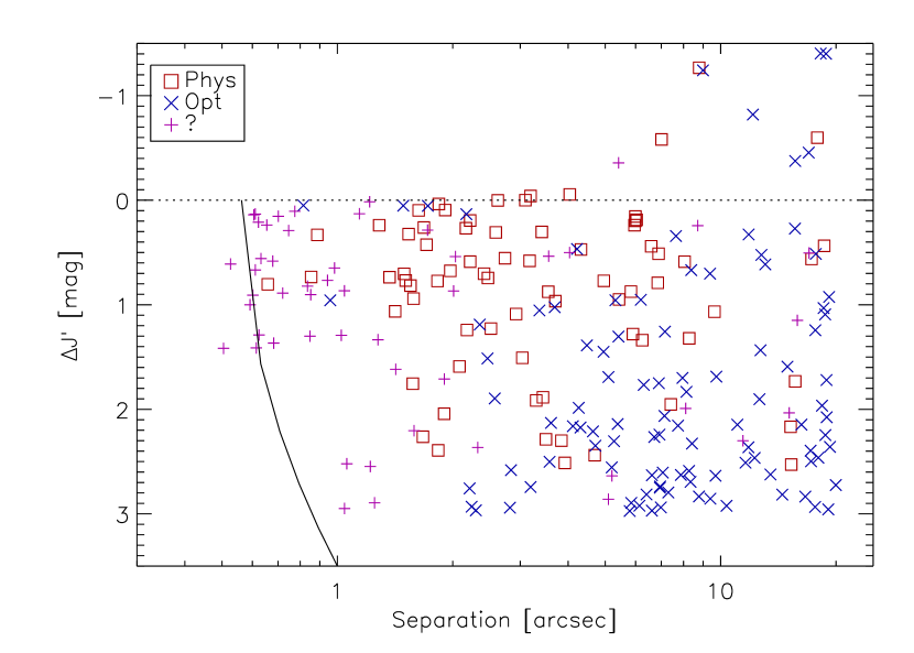
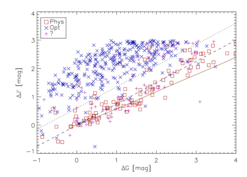
Figure 13.— Distribution of companions in the $(\rho,\Delta J^{\prime})$ plane (top) and in the $(\Delta G,\Delta J^{\prime})$ plane (bottom). Astrometrically confirmed companions are plotted by red squares, non-members by blue crosses, and uncertain companions with $p_{\rm astro}=0.5$ by magenta plus signs. The brown solid line in the lower panel is derived from the 4 Myr PARSEC isochrone for a primary component of 0.6 ${\cal M}_{\odot}$mass.

Table 4Meaning of the $p_{\rm phys}$ flag

$p_{\rm phys}$	$p_{\rm astro}$	$N$	Comment
0	0	397	Astrometric non-members
0.1	0.5	27	Photometric non-members
0.2	1	13	$\rho>7^{\prime\prime}$ photometric non-members
0.3	0.5/1	8	$\Delta J<-0.5$ mag, $\rho>7^{\prime\prime}$
0.8	0.5	5	$\rho<2\arcsec$, $\Delta J<2$ mag, no parallax
0.9	0.5	46	Photometric members
1	1	91	Astrometric members

Figure 13 plots parameters of the companions divided by the $p_{\rm astro}$ flag into three groups: physical, optical, and uncertain. The upper panel shows the expected behavior, where physical pairs concentrate at small separations and small $\Delta J$, optical pairs show the opposite trend, and most uncertain pairs are close, lacking Gaia astrometry for this reason. Note there are several wide ($\rho>7^{\prime\prime}$) pairs in which the secondary components are brighter than the primary, $\Delta J<0$. Some of those companions are astrometrically confirmed members of Ori OB1, meaning that these CVSO targets are the secondary components to brighter stars. Such pairs should not be considered in the statistics. However, in pairs of comparable stars it is difficult to distinguish primary and secondary components, especially considering their variability. We include wide pairs with $\Delta J>-0.5$ mag in our statistics and reject 8 wide pairs with brighter companions.

A physical companion is expected to have a lower temperature and a redder color, compared to the main target. In the lower panel of Figure 13 this trend $\Delta J\approx 0.75\Delta G$ (dashed line) is confirmed. However, the empirical slope of 0.75, chosen to match the trend, is steeper than the slope deduced from the isochrones; in other words, secondary components are slightly bluer than predicted. This trend matches the CMD in Figure 6 where most low-mass stars are located to the left of the isochrones, i.e. have bluer colors. This suggests a potential bias in masses and mass ratios derived from the isochrones.

On the other hand, most optical pairs (blue crosses) are elevated above the $\Delta J=0.75\Delta G$ line by at least 0.6 mag and satisfy the condition

$$\Delta J>0.6+0.75\Delta G$$ (5)

(dotted line in the Figure); most optical companions are bluer than the astrometrically confirmed physical companions. This allows us to classify the pairs that lack good astrometry. We set $p_{\rm phys}=0.9$ for 46 pairs below the dotted line (5) and $p_{\rm phys}=0.1$ for 27 pairs above this line. The close and faint companion to target 1281 (Figure 12) is just above the line and, although possibly physical, it got $p_{\rm phys}=0.1$. Of the 36 pairs with $\rho<2^{\prime\prime}$ lacking reliable GDR2 astrometry, 30 are physical and one optical according to the photometric criterion; five pairs with $\Delta J<2$ mag that lack Gaia photometry are considered likely physical and assigned $p_{\rm phys}=0.8$, based on the low probability of chance projections at close separations. For a typical $J=13$ mag target, we expect to find 2.7 optical companions within 2″ with $\Delta J<2$ mag based on the stellar density in the VISTA Orion catalog, so one or two pairs with $p_{\rm phys}=0.8$ can still be chance alignments.

Selection of physical companions based on the GDR2 astrometry uses rather loose tolerances on the PM and parallax adopted to accommodate effects of unresolved close binaries. One notes in Figure 4 blue and green points (stars with good astrometry) within our selection box but outside the main cluster of points. The astrometric filter alone does not reject all wide ($\rho>7^{\prime\prime}$) optical companions, and we note in Figure 13 several red squares above the dotted line, i.e. photometric non-members; 13 such pairs are assigned $p_{\rm phys}=0.2$ despite their $p_{\rm astro}=1$ flag. Individual examination of their GDR2 astrometry indeed shows that the parallaxes and/or PMs of both components disagree significantly, although both satisfy our loose astrometric membership criteria. Some remaining wide pairs with $p_{\rm astro}=p_{\rm phys}=1$ may still be optical, and we address this issue in the following statistical analysis.

The meaning of the $p_{\rm phys}$ flag and the number of companions in each group are summarized in Table 4. Overall, we consider 142 pairs with $p_{\rm phys}>0.5$ as physical (binaries); 135 of those have main targets that are deemed to be members of Ori OB1. The remaining pairs either are optical (chance projections) or do not belong to Ori OB1.

At wide separations, the contamination by unrelated association members and other stars that pass the astrometric and photometric selection criteria is far from being negligible. The density of these contaminants, or interlopers, must be estimated to make appropriate correction to the binary statistics. The lower limit of 55 stars per square degree is obtained by star counts in the CVSO catalog in section 2.5. The upper limit of $\sim$4000 stars per square degree results from the star count in the Vista Orion catalog. We estimated the realistic density of interlopers by selecting companions in the GDR2 with separations from 20″ to 30″ from our targets that pass the adopted astrometric criteria, ignoring their $r_{\varpi}$. The $J$-band magnitudes of these companions were retrieved from the VISTA Orion catalog by positional match (typically within 0$\farcs$06). The resulting list of 71 companions was further filtered by colors using equation 5, leaving 29 companions with $\Delta J<3$ mag, 24 of those having $\Delta J<2$ mag. Assuming that all those wide companions are interlopers, we derive their density of 226(187) stars per square degree for $\Delta J<3(2)$, respectively. The statistical error of this estimate is about 20%. Considering other uncertainties, we assign the relative error of 30% to the estimated density of interlopers.

3.6. List of binaries in Ori OB1

Table 5Companions with $\Delta J<3$ mag (fragment)

$N$	CVSO	$\theta$	$\rho$	$\Delta J$	$\Delta G$	$p_{\rm astro}$	$p_{\rm phys}$
		(degr)	(″)	(mag)	(mag)
5	427	304.3	16.730	$-$0.41	$-$2.41	0.0	0.0
6	432	101.9	3.440	1.89	2.53	1.0	1.0
8	438	328.9	15.482	2.08	0.45	0.0	0.0
9	439	123.5	17.400	2.16	3.05	0.0	0.0
10	444	303.1	15.419	1.52	0.78	0.0	0.0
11	449	11.3	17.845	2.48	1.00	0.5	0.1
13	453	100.5	16.993	2.94	1.39	0.0	0.0

Figure 14.— Top: comparison of magnitude differences in the $Z$ and $K_{s}$ bands for 86 physical companions with $\rho>2^{\prime\prime}$; the dotted line marks equality. Bottom: Magnitude difference vs. wavelength for physical binaries. Squares plot the median values in each band, the bars show the first and third quartiles.

Multi-band photometry provided by the VISTA Orion survey can potentially help in distinguishing physical and optical pairs. However, magnitudes of a given low-mass young star in all VISTA nIR bands are very similar. The top panel of Figure 14 compares magnitude differences of physical binaries at the shortest and longest VISTA wavelengths. The slope is barely different from one, while the large scatter results from a combination of variability, photometric errors, and/or circumstellar extinction. We base our statistical analysis on the magnitude differences in the $J$ band, which are very close to $\Delta m$ in the adjacent photometric bands $Y$ and $H$. For physical companions, the rms differences between $\Delta m$ in the band $J$ compared to the bands $Z,Y,H,K_{s}$ are 0.38, 0.28, 0.29, and 0.19 mag, respectively. Hence, in the following table we replace $\Delta J$ by $\Delta J^{\prime}$ — the median $\Delta m$ in the $Y,J,H$ bands — in order to reduce random errors and the impact of variability and taking advantage of the fact that there is no systematic difference between $\Delta m$ in these three bands. We use $\Delta J^{\prime}$ in the following in place of $\Delta J$.

Figure 14 illustrates the distributions of $\Delta m$ in six photometric bands for physical binaries by plotting medians and quartiles of the distributions. The distributions in all nIR bands are remarkably similar, with median $\Delta m$ around 0.8 mag. Remember that we keep only pairs with $\Delta J<3$ mag. If the magnitude differences were distributed uniformly, the median would be close to 1.5 mag; instead, real binaries prefer small $\Delta m$. The median $\Delta G=1.2$ mag is larger than in the nIR, as expected for low-mass, low-temperature companions.

The list of 587 companions with $\Delta J<3$ mag found in the images and including wider pairs added from the VISTA Orion catalog is presented in Table 5. Its first four columns are identical to those of Table 3. The next two columns give the magnitude difference $\Delta J^{\prime}$ (median over $Y,J,H$ bands) and the Gaia $\Delta G$. The last columns contain the flags $p_{\rm astro}$ and $p_{\rm phys}$ introduced above. There are 142 likely physical pairs with $p_{\rm phys}>0.5$. To distinguish the 7 physical pairs where the main star is not a member of Ori OB1 (e.g. CVSO 569, see above), their $p_{\rm phys}$ are listed as negative.

3.7. Close binaries observed at SOAR

Figure 15.— Separations $\rho$ and magnitude differences $\Delta I$ of CVSO pairs resolved at SOAR (note: 2 pairs with respective separation of 3$\farcs$7 and 3$\farcs$1 are outside the plotting area). The full and dashed lines show the median detection limit and its quartiles. The separation range between 0$\farcs$15 and 0$\farcs$6 used in the statistical analysis is delimited by the vertical dotted lines.

To probe binary frequency at smaller separations, we observed 123 relatively bright stars in Ori OB1 selected from the CVSO catalog with the speckle camera at the 4.1 m Southern Astrophysical Research (SOAR) telescope in 2016 January. The instrument, data reduction, and results are published in Tokovinin et al. (2019). We detected 28 pairs, including some wide ones also found in the VISTA Orion images (Figure 15). The closest pair has a separation of 0$\farcs$09; 12 pairs have separations between 0$\farcs$15 and 0$\farcs$6, and all these detections are reliable. Some close CVSO pairs discovered in 2016 were confirmed by further speckle observations in 2017–2019. The SOAR data are published and we do not duplicate them here.

Only 74 stars observed at SOAR overlap with the present CVSO-VISTA-Gaia sample, the rest are located outside the sky region studied here. We can use the higher spatial resolution of SOAR observations to double-check VISTA detection sensitivity at small separations, although restricted to the overlap sample. The SOAR observations confirmed that no companions with separations $>$1″ were missed in the VISTA companion search, thereby affirming the assumed completeness for separations $>$1$\farcs$2 and $\Delta J<3$ mag. At smaller separations, i.e. 0$\farcs$6–1$\farcs$2, there is only one binary resolved at SOAR that was missed by VISTA (No. 214, CVSO 2001, 0$\farcs$64, $\Delta I=4.1$ mag, close to or below the VISTA detection limit).

Since this paper is devoted to wide binaries in our well-defined sample, we evoke the SOAR data on closer pairs in a different sample only for reference. The SOAR sample is, on average, brighter than the CVSO-VISTA-Gaia sample. More massive stars are expected to have an increased binary frequency and, indeed, the data hint at a larger companion fraction in the SOAR sample, although the difference is not statistically significant. Moreover, a higher companion fraction among the SOAR sample is naturally expected due to the general shape of the separation distribution that has a peak at $<$100 au.

4. Binary statistics

In this section, we study the statistics of real (physical) binaries with separations from 0$\farcs$6 to 20″ and $\Delta J<3$ mag discovered in the VISTA images and in the VISTA Orion catalog. The parent sample of 1021 members of Ori OB1 contains 135 physical companions, including 4 triples; 131 members have at least one companion. We ignore wide secondary companions that are brighter than our targets by more than 0.5 mag in the $J$ band.

4.1. Distribution of the mass ratio

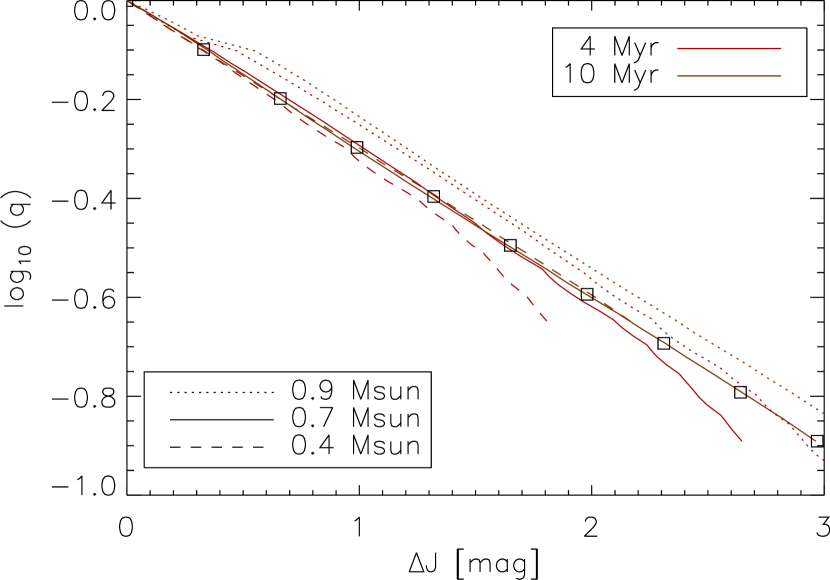
Figure 16.— Relation between $\log_{10}q$ and $\Delta J$ derived from the PARSEC isochrones for primary stars of 0.4, 0.7, and 0.9 ${\cal M}_{\odot}$mass and companions more massive than 0.075 ${\cal M}_{\odot}$. Squares correspond to the linear formula $\log_{10}q=-0.3\Delta J$.

Figure 17.— Cumulative distribution of the mass ratio $q$ for 58 binaries with separations between 1$\farcs$2  and 5″(line and crosses). The dashed and dotted lines correspond to the field binaries (see the text) and to the uniform distribution, respectively.

As noted above, we do not attempt to derive masses and mass ratios. The empirical distribution of mass ratios is evaluated here only to access the fraction of missed companions at close separations and to quantify the survey depth. Fortunately, this fraction and the associated incompleteness correction are small and hence have little influence on our results.

First, we study the distribution of the magnitude difference $\Delta J$ for 57 binaries in the 1$\farcs$2–5″ separation range, where the detection is complete to $\Delta J<3$ mag and the contamination by random pairs of association members is negligible. The distribution is non-uniform, with a preference of small $\Delta J$, as can be inferred by looking at Figure 13. Only 10/58=0.17 fraction of pairs have $2<\Delta J<3$ mag, so by further restricting our analysis to $\Delta J<2$ mag we would reject $\sim$17% of binaries.

The PMS stars and their companions in Orion OB1 are variable. Therefore, there is no unique relation between magnitude difference and mass ratio $q$; for any given binary, different values of $q$ can be inferred from observations at different moments or in different photometric bands. Different circumstellar extinction (so-called infra-red companions) and accretion rates can further complicate translation of relative photometry into $q$. Here we adopt the relation $q\approx 10^{-0.3\Delta J}$ derived from the 4 and 10 Myr isochrones (Figure 16). There is little dependence on the age, except maybe for the youngest and lowest mass stars in Ori OB1b, which represent at most $\sim$15% of the binaries. Our formula is an excellent approximation for 0.7 ${\cal M}_{\odot}$ primary components, roughly equivalent to a spectral type K7-M0, while for 0.9 ${\cal M}_{\odot}$ stars it works less well, with an rms error of 0.06 dex in $\log_{10}q$. For 0.4 ${\cal M}_{\odot}$ stars at 4 Myr the derived mass ratios could be overestimated by 0.1 dex in $\log_{10}q$, but the number of binaries in this parameter space is small; their hydrogen-burning companions have $\Delta J<2$ mag.

The mass ratios deduced by the crude formula from $\Delta J$ appear to be distributed uniformly (Figure 17). Reassuringly, a uniform distribution of $q$ is known to hold for field solar-type binaries (Raghavan et al., 2010; Tokovinin, 2014). El-Badry et al. (2019) studied the mass ratio distribution of wide field binaries, grouping them by the primary mass and separation. They modeled the distribution by a broken power law plus some twins with $q>0.95$. We average the model parameters from their Table F1 in the mass range from 0.4 to 0.8 ${\cal M}_{\odot}$ and the separation range from 600 to 2500 au, roughly matching our survey, and adopt $\gamma_{\rm smallq}=0.25$, $\gamma_{\rm largeq}=-0.8$, and $f_{\rm twin}=0.02$. The corresponding cumulative distribution is over-plotted in Figure 17 by the dashed line; it barely differs from the uniform distribution.

Adopting a uniform distribution of $q$, we evaluate the fraction of missing binaries with small separations using the detection limit $\Delta J(\rho)$ in equation (4). This correction, relevant only at separations below 1$\farcs$2, is small (factor $\sim$1.12, see below). Therefore, our results are little affected by the assumptions regarding the mass ratio conversion and the detection limit.

Table 6Multiplicity on Ori OB1

Separation		Full sample				Ori OB1a			Ori OB1b
′′	au	$N_{i}$	$N^{\prime}_{i}$	$N_{\rm rand}$	$f_{i}$	$N_{i}$	$N^{\prime}_{i}$	$f_{i}$	$N_{i}$	$N^{\prime}_{i}$	$f_{i}$
0.6 – 1.2	314	26	24	0.1	9.4$\pm$1.9	16	16	9.0$\pm$2.3	10	8	10.2$\pm$3.4
1.2 – 2.4	627	33	28	0.2	10.7$\pm$1.9	16	13	8.0$\pm$2.1	17	15	15.5$\pm$3.9
2.4 – 4.8	1255	23	19	1.0	7.2$\pm$1.6	11	10	5.2$\pm$1.8	12	9	10.7$\pm$3.3
4.8 – 9.6	2511	16	16	3.9	3.9$\pm$1.4	10	10	3.8$\pm$1.7	6	6	4.2$\pm$2.5
9.6 – 19.2	5023	31	18	15.5	5.1$\pm$2.4	20	10	5.1$\pm$2.8	11	8	5.0$\pm$3.5
0.6 – 9.6	…	98	87	5.2	9.4$\pm$0.9	53	49	7.8$\pm$1.1	45	38	12.2$\pm$1.8

4.2. Separation distribution and companion fraction

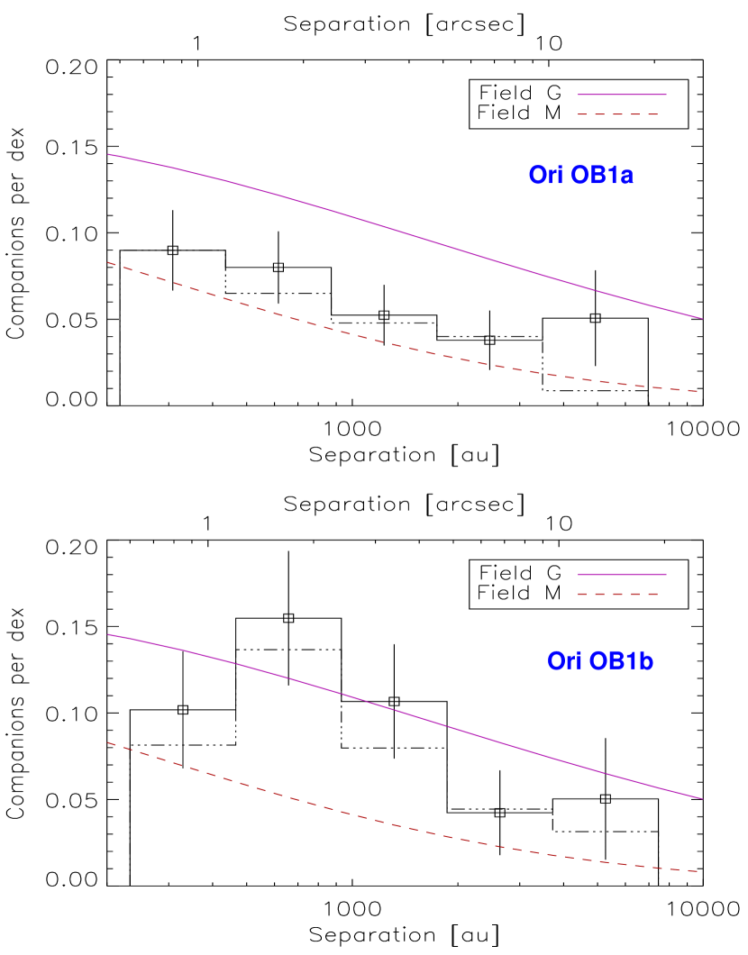
Figure 18.— Companion frequency vs. separation (fraction per decade) in Ori OB1a (top) and Ori OB1b (bottom). The full line corresponds to binaries with $\Delta J<3$ mag, the dash-dot line to binaries with $\Delta J<2$ mag. The log-normal distributions for field stars (solid and dashed curves) are described in the text.

The distribution of separations and the companion frequency are determined in five logarithmic bins of 2$\times$ width covering the separation range from 0$\farcs$6 to 19$\farcs$2 (1.5 dex, 222 to 7104 au at 370 pc distance). Binaries with $\Delta J<3$ mag and $\Delta J<2$ mag are counted in each bin. These numbers $N_{i}$ are used to compute the companion frequency per decade of separation $f_{i}=(N_{i}-N_{\rm rand})/(N_{\rm tot}\log_{10}2)$, where $N_{\rm tot}$ is the sample size. The errors of $f_{i}$ assume the Poisson statistics. The first bin is corrected for undetected companions relatively to other bins; however, this correction is minor, 1.12 and 1.04 times for the two $\Delta J$ thresholds. The expected number of random pairs $N_{\rm rand}$ is estimated from the density of potential contaminants (interlopers) deduced in section 3.5 by selecting companions in the 20″-30″ separation range and applying the same astrometric and photometric filters as used for the closer companions: 226 and 187 stars per square degree for $\Delta J<3$ mag and $\Delta J<2$ mag, respectively; a relative error of 30% is assumed for the density of interlopers and included in the estimated errors of $f_{i}$.

The separation distribution for the full sample and for the OB1a and OB1b groups is given in Table 6, where $N_{i}$ and $N^{\prime}_{i}$ are the numbers of pairs with $\Delta J<3$ mag and $\Delta J<2$ mag, respectively, in each bin and $f_{i}$ are the fractions per decade for $\Delta J<3$ mag in per cent, corrected for incompleteness in the first bin and for the random pairs. The estimated numbers $N_{\rm rand}$ of contaminants with $\Delta J<3$ mag are listed for the full sample. They become comparable to the actual number of companions in the last bin, increasing the $f_{i}$ error. Considering this uncertainty, the last line gives the total number of binaries and the companion frequency in the first four bins only covering 1.2 dex in separation.

The separation distributions in Ori OB1a and Ori OB1b are plotted in Figure 18. Projected separations are translated into au using distances of 363 and 388 pc, respectively (section 2.2); a common distance of 370 pc is used for the full sample. The distributions appear to be different, especially in the second bin, where there are almost twice as many binaries in Ori OB1b as in Ori OB1a. However, bear in mind that the projected separation $s$ equals the semimajor axis $a$ only statistically and their ratio $s/a$ varies by a factor of 2 (i.e. the bin width) both ways owing to projections and random orbital phases. Therefore, even if the distribution of semimajor axes had a sharp feature, it would be spread over adjacent bins in the distribution of $s$. Modeling shows that the distribution of $s/a$ depends on the eccentricity distribution: its median is 0.9 when the average eccentricity is around 0.5 and 0.98 if the eccentricity distribution is linear (thermal), $f(e)=2e$ (see the Appendix). The latter is appropriate for wide binaries considered here (Tokovinin, 2020). Although various correction factors on the order of 1 have been proposed in the literature to convert $s$ into $a$, no correction is actually needed and the statistical distributions of $\log s$ and $\log a$ can be compared directly, provided they are smooth on a $>$0.3 dex scale.

The different multiplicity fractions in both groups can be seen even from the raw numbers. In Ori OB1a, we detect 74 binaries out of 658 targets (multiplicity 11.2$\pm$1.3%). In contrast, in Ori OB1b there are 61 binaries among 363 targets (multiplicity 16.8$\pm$2.2%). The difference of 5.6$\pm$3.2% is significant at the $1.8\sigma$ level. The corrected multiplicity fractions in the last line of Table 6 differ by 4.4$\pm$2.1%, their ratio is 1.6$\pm$0.3.

For reference, we plot in Figure 18 the log-normal distribution for field solar-type binaries derived by Raghavan et al. (2010) with a median of 50 au, separation dispersion of 1.52 dex (2.28 dex in period), and companion frequency of 0.60. The dotted line is the log-normal distribution for field M-type dwarfs found by Winters et al. (2019), with the median at 20 au, dispersion 1.16 dex, and the companion frequency of 0.35, appropriate for early M dwarfs. While the separation distribution of binaries in Ori OB1a is consistent with those of early M-dwarfs, as expected given that the distribution of spectral types in the CVSO sample is weighted to M stars, Ori OB1b shows a high binary fraction, that partially is even higher than for solar-type dwarfs. In both sub-groups of Ori OB1, the companion frequency at separations above $\sim$4000 au (in the last bin) has a large uncertainty caused by the substantial and uncertain fraction of contaminants.

As mentioned above, we refrain from assigning individual masses to the stars of our sample. Instead, we use the $J$-band magnitude as a proxy for mass, in order to explore the dependence of multiplicity on stellar mass. We split the members of Ori OB1 into three equal sets grouped by $J$ magnitude: brighter than $J=12.63$, intermediate, and fainter than $J=13.56$, with 340 stars in each group. The numbers of non-single stars in these groups (61, 48, and 26, respectively, or multiplicity fractions 0.18$\pm$0.023, 0.14$\pm$0.02, and 0.08$\pm$0.016) suggest a substantial dependence of multiplicity on mass, as observed for field binaries.

4.3. Close binaries

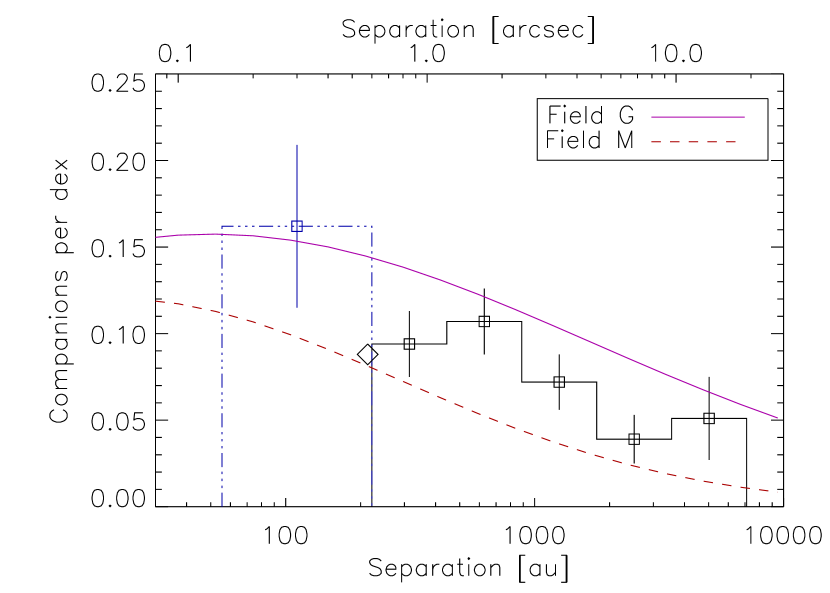
Figure 19.— Distribution of separation in the full sample. The dash-dot line shows the result for the SOAR sample. The diamond is the companion frequency in the ONC from Reipurth et al. (2007). A distance of 370 pc is used.

Figure 19 presents the distribution of projected separations in the full CVSO-VISTA-Gaia sample, including the observed frequency of closer pairs derived from the SOAR observations (the wide dash-dot bar). The latter is $12/123=0.162\pm 0.047$ in the separation range from 0$\farcs$15 to 0$\farcs$6. The faintest companion in this range has a magnitude difference $\Delta I=3.4$ mag. If it is excluded, the binary frequency would be $0.148\pm 0.045$. SOAR observations have variable resolution and contrast sensitivity because they used a laser to correct for atmospheric turbulence and depended on the variable atmospheric conditions. The median detection limit is $\Delta I\sim 2$ mag. Therefore, the SOAR survey is somewhat shallower compared to our survey. The SOAR sample, selected from amongst the brightest CVSO stars, differs from the CVSO-VISTA-Gaia sample in that it contains, on average, brighter, earlier K-type, more massive stars, known to have a larger multiplicity in comparison with late K- and M-type dwarfs. Considering these differences, direct comparison between the SOAR and VISTA Orion multiplicity surveys has to be done with caution. All we can affirm is a qualitative agreement.

Table 7Close binaries in Gaia

Group	$N_{\rm tot}$	No $\varpi$	$r_{\varpi}>2$	$f_{\rm close}$
OB1a	658	25	65	0.137$\pm$0.014
OB1b	363	27	35	0.171$\pm$0.022

Yet another way to probe the frequency of close binaries is offered by Gaia. Stars without measured parallaxes are almost certainly close binaries with separations between 0$\farcs$1 and 0$\farcs$7, as demonstrated, e.g., by Tokovinin & Briceño (2020). Moreover, stars with excess parallax error are also likely close binaries. The total number of these close binary candidates can be used to estimate the frequency of close binaries $f_{\rm close}$, with the caveat that the exact range of separations and mass ratios of these close binaries is not defined and the numbers are not directly comparable to the frequency per decade computed above. The numbers are reported in Table 7. We note the increased fraction of candidate close binaries in Ori OB1b compared to Ori OB1a. This echoes the difference between these groups found for wider pairs, although the difference between the frequency of close Gaia binaries, 3.6$\pm$2.6%, is not statistically significant.

Reipurth et al. (2007) measured the companion frequency for 781 low-mass stars in the periphery of the ONC at projected separations from 67.5 to 675 au and found it to be 8.8$\pm$1.1% (represented by the diamond symbol in Figure 19). Their result agrees, within errors, with the multiplicity in Ori OB1. However, the decline in the binary frequency at separations beyond $\sim$200 au suggested by their study is certainly refuted by our data. Even in the ONC, Jerabkova et al. (2019) found a substantial number of binaries with separations from 1 to 3 kau. The 14 low-mass binaries in the ONC with separations from 30 to 160 au discovered by De Furio et al. (2019) match, within errors, the frequency of M-type binaries in the field.

4.4. Spatial distribution of binaries

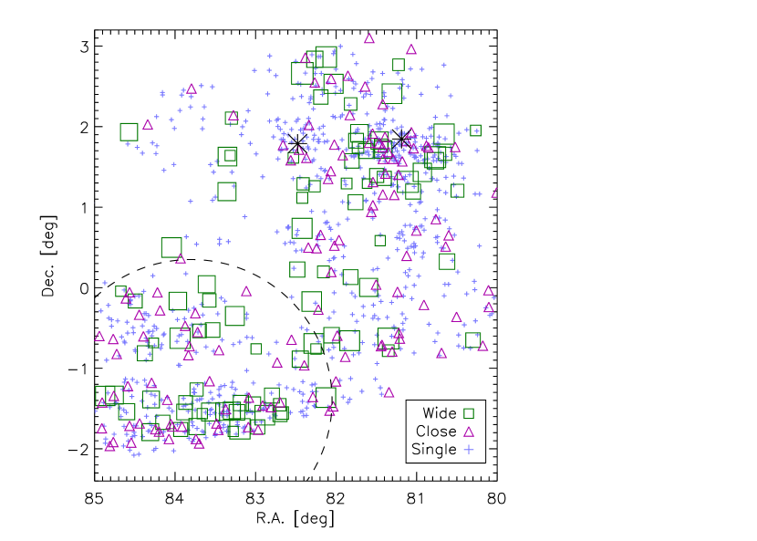
Figure 20.— Spatial distribution of single stars (blue crosses), close Gaia binaries (magenta triangles), and wider VISTA Orion binaries (green squares). The size of the squares reflects binary separation ranging from 0$\farcs$6 to 10″. The two black asterisks show the locations of 25 Ori and HR 1833. The dashed circle depicts the boundary of Ori OB1b.

The difference in the binary statistics between the two subgroups of Orion OB1 is intriguing. To clarify it further, we plot in Figure 20 the spatial distribution of single (i.e. unresolved) stars, wide binaries with separations between 0$\farcs$6 and 10″, and potential close binaries inferred from Gaia. Binaries with separations $>$10″ are ignored because several of them are likely random pairs of association members.

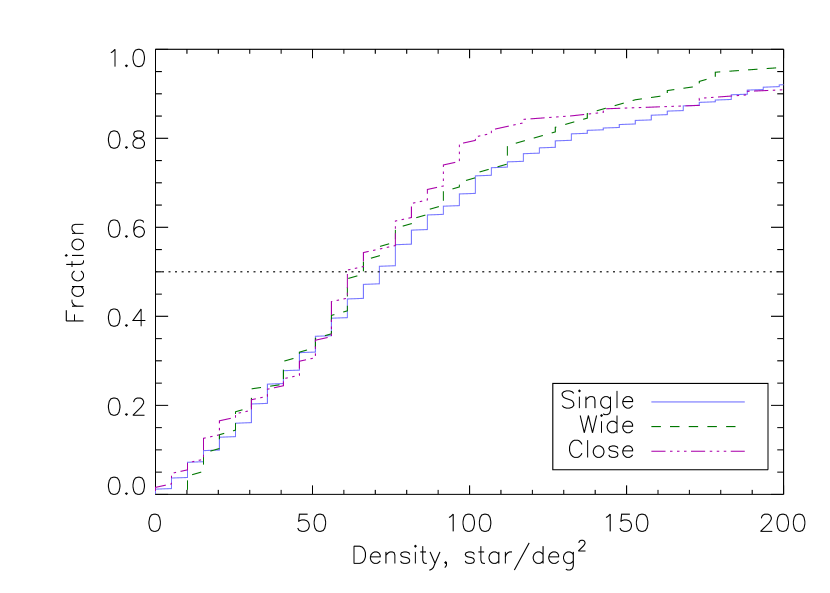
Figure 21.— Cumulative distributions of the density of association members around single stars, wide, and close binaries, computed for 0$\fdg$25 radius.

One notable feature of Figure 20 is the apparent absence of wide binaries in the two stellar over-densities of Ori OB1a near the stars 25 Ori and HR 1833 (marked by asterisks). The latter group lacks wide binaries completely. In the 25 Ori cluster, wide binaries are located on the periphery, at a distance of $\sim$0$\fdg$5 from the central star, and avoid the center. Meanwhile, both clusters contain closer Gaia binaries.

We estimated the mean stellar surface density around each target by counting association members within 0$\fdg$25 radius, which gives an average number of 11 stars in this area. Figure 21 plots the cumulative distribution of surface density in the three groups: single stars, wide binaries with separations between 0$\farcs$6 and 10″, and close binaries inferred from Gaia (763, 97, and 127 stars, respectively). The distributions do not differ significantly (the two-sided Kolmogorov-Smirnov test gives a probability of 0.60 for wide binaries and single stars having the same parent distribution). Therefore, we cannot claim that the frequency of wide binaries in Ori OB1 depends on the stellar density.

On the other hand, the region has dynamically evolved and the density structures seen today most likely differ from the actual birth configuration. Yet, stars in Ori OB1a appear more clustered than those in Ori OB1b, despite being roughly twice the age. Adopting the velocity dispersion in a subgroup of 0.5 mas yr^-1, which corresponds to 0.8 km s^-1, consistent with typical velocity dispersion of young stellar groups and clusters in Orion OB1 (Briceño et al., 2007; Kounkel et al., 2018), we find that in 7 Myr stars can move from their birthplace by $\sim$1°. Stars within $\sim$0$\fdg$5 from the 25 Ori cluster center could have experienced dynamical interactions and been ejected 6-7 Myr ago. This timescale is nicely consistent with the age of the 25 Ori group (Briceño et al., 2019). On the other hand, wide binaries around it could have formed in a low-density environment rather than in the cluster. If the 198 stars located within 0$\fdg$5 from 25 Ori and HR 1833 are removed from the Ori OB1a sample, the frequency of binaries closer than 9$\farcs$6 among the remaining 460 members becomes larger, $\sim$0.1, similar to their frequency in Ori OB1b.

5. Discussion and summary

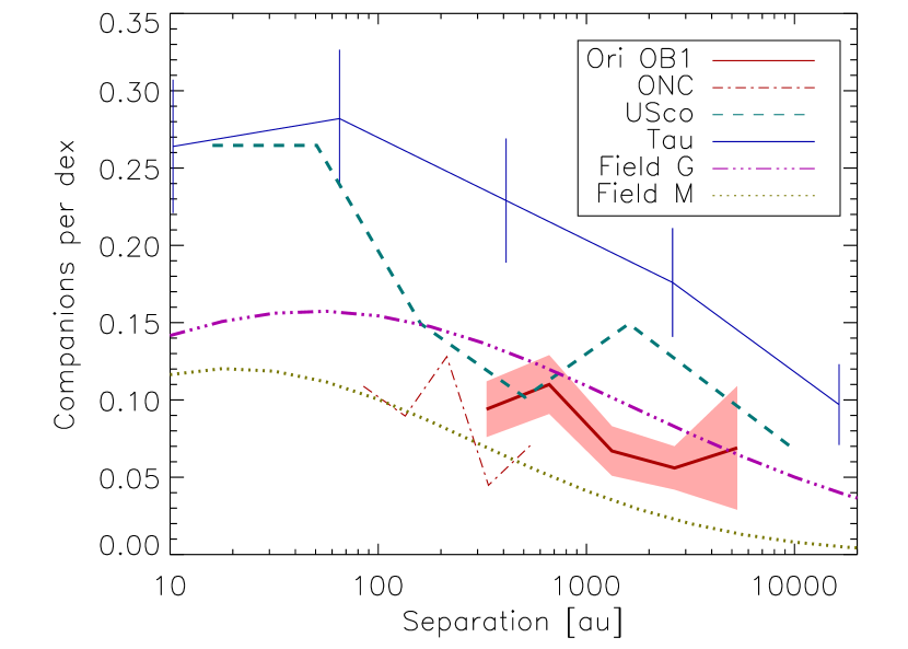
Figure 22.— Comparison of multiplicity in different populations (see text).

In Figure 22 we put our results in the context of multiplicity in other regions, with the obvious caveat related to the differences in the stellar mass range and completeness of various surveys. Assuming a uniform distribution of $q$ between 0.05 and 1, we correct our estimate of multiplicity fraction in Ori OB1 by 0.95/0.9=1.055. The band shows the $1\sigma$ statistical errors. The canonical companion frequency of 0.6 for the field solar-type dwarfs (Raghavan et al., 2010) is assumed. The multiplicity in the Upper Scorpius OB association measured by Tokovinin & Briceño (2020) is similarly corrected by 0.95/0.7=1.36, considering their lower mass ratio limit of $q>0.3$. Their data in the mass range from 0.4 to 1.5 ${\cal M}_{\odot}$ are averaged because no clear dependence of multiplicity on mass was found. We plot the multiplicity in Taurus using the data from Joncour et al. (2017), without any correction. Data from Reipurth et al. (2007) for the ONC are also left uncorrected because the lower limit of the mass ratio in their survey is not known.

The diversity of the multiplicity statistics in young stellar populations, noted already by King et al. (2012) from the scarce data available at the time, is emerging with a stronger confidence from the modern large multiplicity surveys, including this one. In the overall Orion OB1 association the binary fraction is somewhat less than in the field; the opposite is true in Taurus, where the excess of binary fraction over the field is well documented (Duchêne & Kraus, 2013). In the separation range of 1.2 dex from 222 to 3552 au that corresponds to the first four bins in Table 6, the sample of 142 stars in Taurus counts 31 companions (Joncour et al., 2017), hence $f=0.22\pm 0.04$ (the same number can be deduced by summing the last 4 bins of Fig. 4 in Kraus et al., 2011). In Ori OB1, the multiplicity in the same separation range corrected by 1.055 is $0.099\pm 0.009$, and the difference of $0.12\pm 0.04$ is statistically significant. Deacon & Kraus (2020) found a significant deficit of binaries with separations 300–3000 au in open clusters compared to the field and moving groups, confirming the critical role of environment in the binary population statistics.

Considering Ori OB1a and OB1b individually, we note that OB1b shows a binary fraction comparable to the field and is more similar to Upper Scorpius, at least for the wide binaries that we probe in our study. There is accumulating evidence that Upper Scorpius, as well as other OB associations, most likely were formed in a configuration similar to how they appear today — i.e. as an assembly of loose stellar groups with moderate to low stellar density (Wright & Mamajek, 2018; Lim et al., 2019). If the initial stellar density of a star forming environment largely dictates the formation or dynamical destruction of wide binaries, one might speculate that a different stellar birth density causes the observed difference in binary fraction between Ori OB1a and Ori OB1b. In this picture Ori OB1a would have formed from a dense cluster, while Ori OB1b would stem from a wide-spread population with only some sparsely clustered substructures. Future kinematic studies with Gaia providing higher precision than GDR2 will hopefully allow to further explore this issue. Regarding the origin of the field binaries, a mix of Orion-type and Taurus-type binary populations in a suitable proportion would resemble the field.

The main results of our study are as follows:

• Double stars in a sample of 1021 low-mass PMS stars of the Orion OB1 association, selected from the CVSO catalog, have been identified by the analysis of the nIR images from the VISTA Orion mini-survey. Using Gaia astrometry and photometry, we rejected unrelated pairs and arrived at a list of 135 most likely real (physical) companions, arranged in 127 binaries and 4 triples, with projected separations from 0$\farcs$6 to 20″(222 – 7400 au at 370 pc) and magnitude difference $\Delta J<3$ mag.

• The distribution of magnitude difference $\Delta J$ of these binaries is compatible with a uniform mass ratio distribution. Our survey is almost complete for wide binaries with mass ratios above 0.13.

• We found that the two sub-groups, Ori OB1a and Ori OB1b, likely have a different multiplicity rate: 0.078$\pm$0.011 and 0.122$\pm$0.018, respectively, in the 1.2 dex separation range from 0$\farcs$6 to 9$\farcs$6 (222 to 3600 au at 370 pc).

• The frequency of wide binaries in Ori OB1 depends on mass (more companions around more massive stars similarly to the field) but is independent of the currently observed surface density of stars. Location of wide binaries on the sky suggests that they avoid cluster centers.

• Our survey highlights the differences in multiplicity properties between star-forming regions. The binary population in the field could result from a mixture of these diverse populations.

Appendix A Relation between projected separation and semimajor axis

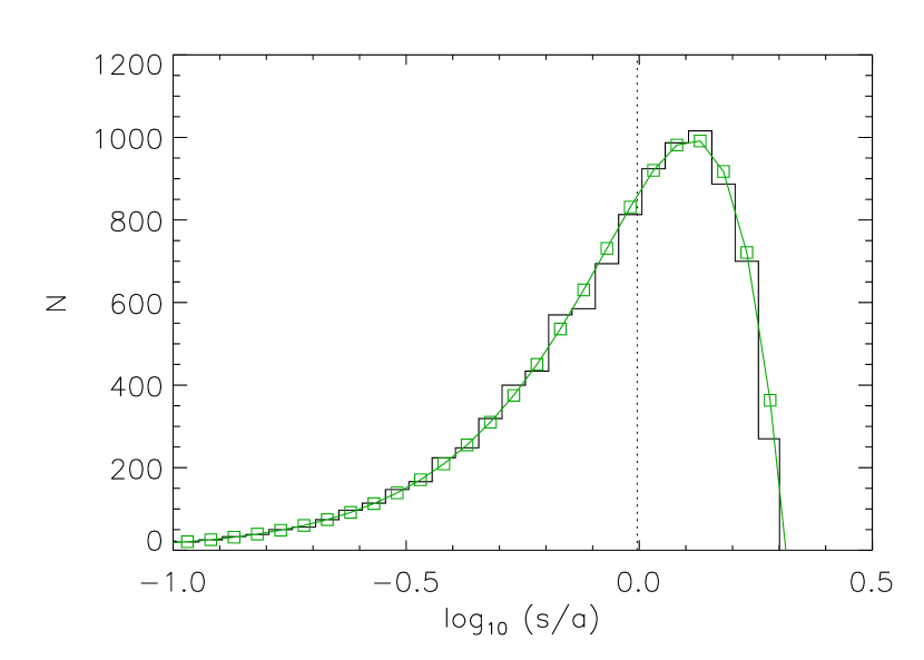
Figure 23.— Left: cumulative distribution of the ratio $s/a$ (line) and its analytic model (squares) for thermal eccentricity distribution. Right: histogram of the same data and their model (green squares and line); vertical dotted line marks the median.

On Referee’s request, we include a short discussion of the statistical relation between projected separation $s$ used throughout this paper and the true semimajor axis $a$ of the binary orbit. The ratio $x=s/a$ is computed for $10^{4}$ simulated binaries with random orbit orientation and random phase. The resulting distribution of $x$ slightly depends on the adopted eccentricity distribution; here we assume the thermal distribution $f(e)=2e$ appropriate for wide binaries. Figure 23 (left) shows the cumulative distribution of $x$ for simulated binaries and its analytic model

$$F(x)=0.5+0.5\sin[\pi/2\;(x/x_{0})^{\alpha}],$$ (A1)

where $x_{0}=0.98$ is the median and $\alpha=0.94$ encodes deviation from the pure sine curve. These parameters were fitted to the simulated distribution. The analytical model (A1) is remarkably good, with rms deviation of 0.0005 and the maximum deviation of 0.005. If a uniform eccentricity distribution is assumed, the fitted parameters are $x_{0}=0.92$ and $\alpha=1.05$, but the difference between distribution and its model is $\sim$6$\times$ larger than for thermal eccentricities.

For a thermal eccentricity distribution, the median projected separation $s$ is an accurate measure of the true median semimajor axis, no correction is needed. In a sample of binaries, 82.8% of projected separations differ from the true semimajor axis by a factor less than two, and the remaining 17.2% have $s<0.5a$.

Multiplicative factors slightly larger than one have been proposed in the literature to convert $s$ into $a$ (e.g. Raghavan et al., 2010). Different values of scaling factors are obtained depending on the assumed eccentricity distribution and on the metric used to compute the factor (median, mean $s/a$, mean $a/s$, mean $\log a/s$, etc.). The distribution of $s/a$ in Figure 23 is almost symmetric, its mean is very close to the median. However, the distribution of the logarithm is skewed, and $\langle\log(s/a)\rangle=-0.073$ might suggest $a\approx 1.18s$, while $\langle a/s\rangle=1.59$. The correct approach is to de-convolve the observed distributions of $s$ from projection using the kernel from simulations (or its analytical approximation), instead of simple scaling. Example of such deconvolution is provided in the Appendix of (Tokovinin, 2018).

References

- Blaauw (1964) Blaauw, A. 1964, ARA&A, 2, 213
- Brandeker & Cataldi (2019) Brandeker, A. & Cataldi, G. 2019, A&A, 621, A86
- Briceño et al. (2005) Briceño, C., Calvet, N., Hernández, J., et al. 2005, AJ, 129, 907
- Briceño et al. (2007) Briceño, C., Hartmann, L., Hernández, J., et al. 2007, ApJ, 661, 1119
- Briceño et al. (2019) Briceño, C., Calvet, N., Hernández, J., et al. 2019, AJ, 157, 85
- Chen et al. (2019) Chen, B., D’Onghia, E., Alves, J., & Adamo, A. 2019, eprint arXiv:1905.11429
- Danielsky et al. (2018) Danielsky, C., Barbuisaux, C., Ruiz-Dern, L., et al. 2018, A&A, 614, 19
- Deacon & Kraus (2020) Deacon, N. R. & Kraus, A. L. 2020, MNRAS, 496, 5176
- De Furio et al. (2019) De Furio, M., Reiter, M., Meyer, M. R., et al. 2019, ApJ, 886, 95
- Duchêne & Kraus (2013) Duchêne, G. & Kraus, A. 2013, ARA&A, 51, 269
- Duchêne et al. (2018) Duchêne, G., Lacour, S., Moraux, E., et al. 2018, MNRAS, 478, 1825
- El-Badry et al. (2019) El-Badry, K., Rix, H.-W. & Tian, H. 2019, MNRAS, 489, 5822
- Gaia collaboration (2018) Gaia Collaboration, Brown, A. G. A., Vallenari, A., Prusti, T., et al. 2018, A&A, 595A, 2 (Vizier Catalog I/345/gaia2; GDR2).
- Fabricant et al. (2005) Fabricant D., Fata, R., Roll, J., et al. 2005, PASP, 117, 1411
- Jerabkova et al. (2019) Jerabkova, T., Beccari, G., Boffin, H. M. J., et al. 2019, A&A, 627, 57
- Joncour et al. (2017) Joncour, I., Duchêne, G. & Moraux, E. 2017, A&A, 599, 14
- King et al. (2012) King, R. R., Goodwin, S. P., Parker, R. J., & Patience, J. 2012, MNRAS, 427, 2036
- Kos et al. (2019) Kos, J., Bland-Hawthorn, J., Asplund, M., et al. 2019, A&A, 631, 166
- Kounkel et al. (2018) Kounkel, M., Covey, K., Suárez, G., et al. 2018, AJ, 156, 84
- Kraus et al. (2011) Kraus, A., Ireland, M. J., Martinache, F., & Hillenbrandt, L. A. 2011, ApJ, 731, 8
- Larson (1995) Larson, R. B. 1995, MNRAS, 272, 213
- Lim et al. (2019) Lim, B., Nazé, Y., Gosset, E., & Rauw, G. 2019, MNRAS, 490, 440
- Maddalena et al. (1986) Maddalena, R. J., Morris, M., Moscowitz, J., & Thaddeus, P., 1986, ApJ, 303, 375
- Monet (1998) Monet, D. 1998, USNO-A2.0
- Parker & Meyer (2014) Parker, R. J., & Meyer, M. R. 2014, MNRAS, 442, 3722
- Petr-Gotzens et al. (2011) Petr-Gotzens, M., Alcalá, J. M., Briceño, C., et al. 2011, Messenger, 145, 29
- Raghavan et al. (2010) Raghavan, D., McAlister, H. A., Henry, T. J., et al. 2010, ApJS, 190, 1
- Reipurth et al. (2007) Reipurth, B., Guimarães, M. M., Conneley, M., & Mally, J. 2007, AJ, 134, 2272
- Skrutskie et al. (2006) Skrutskie, M. F., Cutri, R. M., Stiening, R., et al. 2006, AJ, 131, 1163
- Spezzi et al. (2015) Spezzi, L., Petr-Gotzens, M. G., Alcalá, J. M., et al. 2015, A&A, 581, A140
- Tang et al. (2014) Tang, J., Bressan, A., Rosenfield, P., et al. 2014, MNRAS, 445, 4287
- Taylor (2005) Taylor, M. B. 2005, Astronomical Data Analysis Software and Systems XIV, 29
- Tokovinin (2014) Tokovinin, A. 2014, AJ, 147, 87
- Tokovinin (2018) Tokovinin, A. 2018, ApJS, 235, 6
- Tokovinin (2020) Tokovinin, A. 2020, MNRAS, 496, 987
- Tokovinin & Briceño (2020) Tokovinin, A. & Briceño, C. 2020, AJ, 159, 15
- Tokovinin et al. (2019) Tokovinin, A., Mason, B. D., Mendez, R. A., et al. 2019, AJ, 158, 48
- Warren & Hesser (1977) Warren, W. H. & Hesser, J. E. 1977, ApJS, 34, 115
- Winters et al. (2019) Winters, J. G., Henry, T. J., Wei-Chun, J., et al. 2019, AJ, 157, 216
- Wright & Mamajek (2018) Wright, N. J. & Mamajek, E. E. 2018, MNRAS, 476, 381
- Zacharias et al. (2013) Zacharias, N., Finch, C., Girard, T., et al. 2013, AJ, 145, 44
- Zari et al. (2019) Zari, E., Brown, A. G. D. & de Zeeuw, P. T. 2019, A&A, 628, 123