The sum of the masses of the Milky Way and M31: a likelihood-free inference approach

Abstract

We use Density Estimation Likelihood-Free Inference, $\Lambda$ Cold Dark Matter simulations of $\sim 2M$ galaxy pairs, and data from Gaia and the Hubble Space Telescope to infer the sum of the masses of the Milky Way and Andromeda (M31) galaxies, the two main components of the Local Group. This method overcomes most of the approximations of the traditional timing argument, makes the writing of a theoretical likelihood unnecessary, and allows the non-linear modelling of observational errors that take into account correlations in the data and non-Gaussian distributions. We obtain an $M_{200}$ mass estimate $M_{\rm MW+M31}=$ $4.6^{+2.3}_{-1.8}\times 10^{12}\text{\,}\mathrm{\mathit{M_{\odot}}}$ ($68\%$ C.L.), in agreement with previous estimates both for the sum of the two masses and for the individual masses. This result is not only one of the most reliable estimates of the sum of the two masses to date, but is also an illustration of likelihood-free inference in a problem with only one parameter and only three data points.

I Introduction

Likelihood-free inference (LFI) has emerged as a very promising technique for inferring parameters from data, particularly in cosmology. It provides parameter posterior probability estimation without requiring the calculation of an analytic likelihood (i.e. the probability of the data being observed given the parameters). LFI uses forward simulations in place of an analytic likelihood function. Writing a likelihood for cosmological observables can be extremely complex, often requiring the solution of Boltzmann equations, as well as approximations for highly nonlinear processes such as structure formation and baryonic feedback. While simulations have their own limitations and are computationally expensive, the quality and efficiency of cosmological simulations are constantly increasing, and they are likely to soon far surpass the accuracy or robustness of any likelihood function.

This is a rapidly growing topic in cosmology, due to the emergence of novel methods for likelihood-free inference (see e.g. Leclercq, 2018; Alsing et al., 2019), with applications to data sets such as the Joint Light Curve (JLA) and Pantheon supernova datasets (Betoule et al., 2014; Wang et al., 2020), and the Dark Energy Survey Science Verification data (Jeffrey et al., 2020), amongst others (Brehmer et al., 2019; Ramanah et al., 2020; Tortorelli et al., 2020). There are, therefore, many applications for which LFI could improve the robustness of parameter inference using cosmological data. In this work we perform a LFI-based parameter estimation of the sum of masses of the Milky Way and M31. The likelihood function for this problem requires significant simplifications, but forward simulations can be obtained easily.

The Milky Way and Andromeda are the main components of the Local Group, which includes tens of smaller galaxies. We define $M_{\rm MW+M31}$ as the sum of the MW and M31 masses. Estimating $M_{\rm MW+M31}$ remains an elusive and complex problem in astrophysics. As the mass of each of the Milky Way and M31 is known only to within a factor of 2, it is important to constrain the sum of their masses. The traditional approach is to use the so-called timing argument (TA) (Kahn and Woltjer, 1959). The timing argument estimates $M_{\rm MW+M31}$ using Newtonian Dynamics integrated from the Big Bang. This integration is an extremely simplified version of a very complex problem. Therefore, alternative methods that do not rely on the same approximations become extremely useful.

In this work, we use the MultiDark Planck (MDPL) simulation Prada et al. (2012); Riebe et al. (2013), combined with data from the Hubble Space Telescope (HST, Meylan et al., 2004) and Gaia (Gaia Collaboration, 2016), to estimate $M_{\rm MW+M31}$. A similar data set was previously used in (McLeod et al., 2017) to obtain a point estimate of $M_{\rm MW+M31}$ using Artificial Neural Networks (ANN) in conjunction with the TA. In contrast, our work uses Density Estimation Likelihood-Free Inference (DELFI Bonassi et al., 2011; Fan et al., 2012; Papamakarios and Murray, 2016; Alsing et al., 2019), using the pyDELFI package, combined with more recent data. While the result is important on its own, this paper also illustrates the fundamental methodology of DELFI in a problem that is statistically simple but physically complex.

The structure of the paper is as follows: Sec. II reviews and describes previous estimates of $M_{\rm MW+M31}$. Sec. III describes the basics of LFI, and the particular techniques used in this work. Sec. IV and Sec. V describe the simulations and data, respectively, used in this work. Sec. VI shows our results, and conclusions are presented in Sec. VII.

II Previous Estimates

Table 1: Estimates of $M_{\rm MW+M31}$ from previous work. The third column shows the data used, with $r$ in $\mathrm{Mpc}$ and $v_{r},v_{t}$ in $\mathrm{km}\text{\,}{\mathrm{s}}^{-1}$. The fourth column shows $M_{\rm MW+M31}$ in units of $\mathrm{1}\mathrm{0}^{12}\mathrm{\mathit{M_{\odot}}}$. Note that Gaussian approximations have been used to convert the reported confidence levels to $68\%$ confidence levels in some cases.

Reference	method	assumed ($r,v_{r},v_{t}$ )	$M_{\rm MW+M31}$
Li & White (2008) (Li and White, 2008)	TA calibrated on Sims	(0.784, 130, 0)	$5.27^{+2.48}_{-0.91}$
Gonzalez & Kravtsov (2014) (Gonzalez et al., 2014)	Sims	(0.783, 109.3, 0)	$4.2^{+2.1}_{-1.2}$
McLeod et al. (2017) (McLeod et al., 2017)	TA+$\Lambda$	($0.77\pm 0.04,109.4\pm 4.4,17\pm 17$)	$4.7^{+0.7+2.9}_{-0.6-1.8}$
McLeod et al. (2017) (McLeod et al., 2017)	Sims + ANN +Shear	($0.77\pm 0.04,109.4\pm 4.4,17\pm 17$)	$4.9^{+0.8+1.7}_{-0.8-1.3}$
Phelps et al. (2013) (Phelps et al., 2013)	Least Action	(0.79, 119, 0)	$6.0\pm 0.5$

A first approach to estimating $M_{\rm MW+M31}$ from dynamics, known as TA, is based on the simple idea that MW and M31 are point masses approaching each other on a radial orbit that obeys

$$\ddot{r}=-\frac{GM_{\rm MW+M31}}{r^{2}}+\frac{1}{3}\Lambda\,r,$$ (1)

where $M_{\rm MW+M31}$ is the sum of the masses of the two galaxies (Kahn and Woltjer, 1959; Lynden-Bell, 1981), and where the $\Lambda$ term, which represents a form of dark energy, was added in later studies (Binney and Tremaine, 1987; Partridge et al., 2013). It was also extended for modified gravity models (McLeod and Lahav, 2019). Since we know the present-day distance $r$ between MW and M31 and their relative radial velocity $v_{r}$, and if we assume the age of the universe and $\Lambda$, we can infer the mass $M_{\rm MW+M31}$. The analysis can be extended to cover the case of non-zero tangential $v_{t}$ velocity (e.g. McLeod et al., 2017; Benisty et al., 2019). The pros and cons of the timing argument are well known. It is a simple model which assumes only two point mass bodies; this ignores, for example, the tidal forces due to neighbouring galaxy haloes in the Local Group and the extended cosmic web around it. While the timing argument model does not capture the complexity of the cosmic structure and resulting cosmic variance, it gives a somewhat surprisingly good estimate for $M_{\rm MW+M31}$. As shown below, it can also serve to test the sensitivity of the results to parameters such as the cosmological constant $\Lambda$ and the Hubble constant $H_{0}$, in case simulations are not available for different values of these parameters.

A second approach is to consider the dynamics of all the galaxies in the Local Group using the Least Action Principle (Peebles, 1994), as, for example, was implemented in Phelps et al. (2013). In this approach all members of the Local Group appear in the model, but as a result the derived masses are correlated, and the error bars should be interpreted accordingly. A third approach is to use N-body simulations of the local universe, assuming a cosmological model such as $\mathrm{\Lambda CDM}$ (Li and White, 2008; Gonzalez et al., 2014; McLeod et al., 2017). In this paper we apply this third method, but using the DELFI method (this provides significant improvements over other methods, as discussed in the following section).

Representative results for $M_{\rm MW+M31}$ from previous works are given in Tab. 1. Throughout the paper we quote $68\%$ credible intervals.

III Likelihood-Free Inference

In Bayesian statistics we often face the following problem: given observed data $D_{\rm obs}$, and a theoretical model $I$ with a set of parameters $\theta$, calculate the probability of the parameters given the data. In other words, we want to calculate the posterior distribution $\mathcal{P}\equiv p(\theta|D_{\rm obs},I)$; here $p$ is a probability (for a model with discrete parameters) or a probability density (for continuous parameters). We do so using Bayes’ theorem:

$$p(\theta|D_{\rm obs},I)={p(D_{\rm obs}|\theta,I)p(\theta|I)\over p(D_{\rm obs}|I)}\Leftrightarrow\mathcal{P}={\mathcal{L}\times\Pi\over\mathcal{Z}}$$ (2)

where $\mathcal{L}$ is called the likelihood, $\Pi$ the prior, and $\mathcal{Z}$ the Bayesian Evidence. The Bayesian Evidence acts as an overall normalization in parameter estimation, and can therefore be ignored for this task. Thus, given a choice of prior distribution and a likelihood function, we can estimate the posterior distribution. However, obtaining a likelihood function is not always easy. The likelihood function provides a probability of measuring the data as a function of the parameter values, and often requires approximations both in the statistics and in the theoretical modelling.

Likelihood-Free Inference is an alternative method for calculating the posterior distribution; in this method we do not formally write down a likelihood function. Instead, we use forward simulations of the model to generate samples of the data and parameters. In the simplest version of LFI, we select only the forward simulations that are the most similar to the observed data, rejecting the rest. This method is known as Approximate Bayesian Computation (ABC, Rubin, 1984); it relies on choices of a distance metric (to measure similarity between simulated and observed data) and of a maximum distance parameter $\epsilon$ (used to accept or rejected simulations).

In this work, we will use a version of LFI called Density Estimation Likelihood-Free Inference (DELFI). In this approach, we use all existing forward simulations to learn a conditional density distribution of the data $d$ given the parameters $\theta$, using a density estimation algorithm. Examples of density estimation algorithms are Kernel Density Estimation (KDE, Rosenblatt, ; Parzen, ; Simonoff, 1996), Mixture Models, Mixture Density Networks (Bishop, 1994, 2006), and Masked Autoregressive Flows (Papamakarios et al., 2017). We use the package pyDELFI, and estimate the likelihood function from the forward simulations using Gaussian Mixture Density Networks (GMDN) and Masked Autoregressive Flows (MAF). In this sense, the name Likelihood-Free Inference is perhaps misleading: the inference is not ‘likelihood-free’, we simply avoid writing a likelihood and instead model it using forward simulations. A more accurate name for the method could therefore be ‘explicit-likelihood-free’. A more extended discussion of our choice of density estimation algorithms and conditional distribution is presented in Appendix A.

DELFI has several advantages over the simpler ABC approach to LFI: it does not rely on a choice of a distance parameter $\epsilon$ (although admittedly the choice of basis in parameter space can change the implicit distance metric of the density estimator) and it uses all available forward simulations to build the conditional distribution, making it far more efficient.

While relatively new, likelihood-free inference has already been applied to several problems in astrophysics (e.g. Cameron and Pettitt, 2012; Weyant et al., 2013; Akeret et al., 2015; Hahn et al., 2017; Peel et al., 2017; Kacprzak et al., 2018; Jeffrey et al., 2020). However, most applications involving LFI suffer from the curse of dimensionality: there can be hundreds, thousands, or even millions of observables (such as $\sim 2000$ multipoles in Cosmic Microwave Background surveys, or $~{}500$ redshift and angular bins in cosmic shear analyses), and it is impossible to perform density estimation. Some form of data compression is therefore usually needed (Alsing et al., 2018; Alsing and Wandelt, 2018; Heavens et al., 2020). Similarly, due to the high dimensionality and complexity of these parameter spaces, efficient methods to generate the simulations (so as to minimize the number needed) have been developed (Papamakarios et al., 2019; Lueckmann et al., 2019; Alsing et al., 2019). However, our $M_{\rm MW+M31}$ problem has only three data points and one parameter of interest, making it an extremely simple application of the method from the statistical point of view; it illustrates all necessary techniques, and does not require data compression.

To summarize, the steps that we will follow are:

• Generate a large number of simulations of systems similar to the one of interest. The simulations used in this work are described in Sec. IV.

• Use a density estimator, in our case GMDN and MAF as part of the pyDELFI package, to obtain the sampling distribution for any data realization $p(d|\theta,I)$.

• Evaluate this distribution at the observed data (which will be described in Sec. V) to obtain the likelihood function for our observed data realization: $p(d=D_{\rm obs}|\theta,I)$.

• From a prior distribution and the likelihood, and using Bayes’ theorem (Eq. 2), get a posterior distribution $p(\theta|D_{\rm obs},I)$.

IV Simulations

We use the publicly available MDPL simulation. This is an $N$-body simulation of a periodic box with side length $L_{\rm box}=$ $1\text{\,}\mathrm{Gpc}\text{\,}{\mathrm{\mathit{h}}}^{-1}$, populated with $2048^{3}$ dark matter particles. Such a simulation achieves a mass resolution of $8.7\text{\times}{10}^{9}\text{\,}\mathrm{\mathit{M_{\odot}}}\text{\,}{\mathrm{\mathit{h}}}^{-1}$ and a Plummer equivalent gravitational softening of $7\text{\,}\mathrm{kpc}$. The simulation was run with the ART code and assumed a $\Lambda$CDM power spectrum of fluctuations with $\Omega_{\Lambda}=0.73$, $\Omega_{\rm b}=0.047$, $\Omega_{\rm m}=0.27$, $\sigma_{\rm 8}=8.2$ and $H_{0}=$100\text{\,}\mathrm{\mathit{h}}\text{\,}\mathrm{km}\text{\,}{\mathrm{s}}^{-1}\text{\,}{\mathrm{Mpc}}^{-1}$$, with $h=0.7$.

Haloes are identified with the AHF halo finder (Knebe et al., 2011). AHF identifies local over-densities in the density field as possible halo centres. The local potential minimum is computed for each density peak and the particles that are gravitationally bound are identified. Haloes with more than 20 particles are recorded in the halo catalogue. The AHF catalogue includes some 11,960,882 dark matter haloes.

The halo catalogue is then searched for pairs of galaxies as follows. We first identify those haloes in the mass range $5\times 10^{10}<M/M_{\odot}h^{-1}<5\times 10^{13}$. For each such halo, we find all haloes (irrespective of mass) within $\sim$$4\text{\,}\mathrm{Mpc}$ and sort these by distance. If the closest of these is within the mass range $[5\times 10^{10},5\times 10^{13}]$ and is separated by more than $500\text{\,}\mathrm{kpc}$ but less than $1500\text{\,}\mathrm{kpc}$, the two haloes are considered a potential pair. The partner is then examined to ensure that the pair is isolated (namely that there is no other halo with a mass $>5\times 10^{10}$ and closer to either pair member than the pair separation). If this is the case then the pair is kept for the analysis described here. In this way, 1,094,839 pairs are found (as opposed to the $30,190$ pairs used in (McLeod et al., 2017)).

We believe the criteria used to select the halo pairs in this work are not very restrictive and any cuts lie well outside the realistic limits for the actual MW-M31 system. Though these selections are unrestrictive, we note that including more pairs does improve the density estimation, as DELFI can use all the available simulated data, and not only those that are close to the observation.

V Data

Figure 1: An illustration of our non-Gaussian error modelling for the tangential velocity. The plot was obtained taking the components of the tangential velocity for a randomly chosen simulation (with fixed $M$), scattering a large number of times by the errors of Eq. 3, and calculating the norm for each sample. The black dashed line shows the norm of the components for the tangential velocity of the simulation without measurement error.

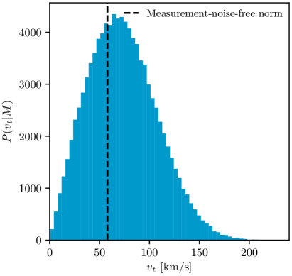
We use three observations to constrain $M_{\rm MW+M31}$: the distance to M31, and the radial and tangential components of its velocity. While the TA requires other observables, such as the age of the Universe $t_{0}$ and the cosmological constant $\Lambda$, in our approach these are already included in the simulations at fixed values. We discuss below how uncertainties in cosmological parameters affect the estimated mass.

For the distance to M31, we adopt the commonly used value $r=$ $770\pm 40\text{\,}\mathrm{kpc}$ (Holland, 1998; Joshi et al., 2003; Ribas et al., 2005; McConnachie and Irwin, 2006). For the velocity, we follow the results of (van der Marel et al., 2019, henceforth VdM19). The radial velocity in the galactocentric rest frame is $v_{r}=$-109.4\pm 4.4\text{\,}\mathrm{km}\text{\,}{\mathrm{s}}^{-1}$$ (van der Marel et al., 2012) from HST observations. The tangential velocity is slightly more cumbersome. VdM19 report the following value for components of the tangential velocity of M31 from a combination of Gaia DR2 and HST:

$$\mu=\left(10\pm 11,-16\pm 11\right)$\mathrm{\SIUnitSymbolMicro as}\text{\,}{\mathrm{yr}}^{-1}$,$$ (3)

already in the galactocentric frame, i.e. after correcting for the solar reflex motion. VdM19 uses the distance to M31 to convert this to $\mathrm{km}\text{\,}{\mathrm{s}}^{-1}$. They then use a method described in (van der Marel and Guhathakurta, 2008) to correct for the fact that taking the norm of the two components leads to a ‘bias’ in the reported tangential velocity. However, in this work, we take a different approach: for each simulation, we scatter the value of each component of the tangential velocity for the simulation according the observational error of each components shown in Eq. 3. By doing this, we are putting the observational errors in the simulated measurements, instead attempting to ‘debias’ the tangential velocity summary statistic. We convert to $\mathrm{km}\text{\,}{\mathrm{s}}^{-1}$ using the value of the distance for that sample, to account for the covariance between $r$ and $v_{t}$. We take as the observed value the norm of the two observed components, $v_{t}=$ $72\text{\,}\mathrm{km}\text{\,}{\mathrm{s}}^{-1}$. While this differs from the value reported in VdM19, this should not be a problem, as long as the way in which we calculate the tangential velocity in simulations and observations is consistent, and we use a summary statistic that extracts all the available information (which the norm of the components does). Furthermore, Appendix C shows that our results do not significantly change if we repeat the analysis using a purely radial motion ($v_{t}=0$).

This approach takes into account both the non-Gaussian errors in $v_{t}$ and the correlation of $v_{t}$ with the errors in the distance measurement (these have not been accounted for in previous estimates of $M_{\rm MW+M31}$).

VI Results

VI.1 Overview

Figure 2: Illustration of DELFI for the estimation of $M_{\rm MW+M31}$. The left panel is a scatter plot of the simulations described in Sec. IV. The right panel adds the observational errors by scattering the simulations.

Figure 3: Conditional distribution $p(d|\theta,I)$ density estimate from the points shown in the right panel of Fig. 2. The 2D subplots in the left column show the probabilities of the data $d=\left\{r,v_{r},v_{t}\right\}$ conditional on the parameter $\theta=M$ (which has been given a uniform distribution), while the remaining 2D subplots have been marginalised over this uniform distribution. By evaluating this function at the observed data points $d=\left\{r,v_{r},v_{t}\right\}$ we obtain the likelihood function. The points were sampled using the Nested Sampling (Skilling et al., 2006) code PolyChord (Handley et al., 2015a, b). Note that the one dimensional distribution on $M$ is flat by construction, as this is the parameter, and the distributions on $r$ and $v_{r}$ appear to be ‘cut’ because of the selection criteria described in Sec. IV.

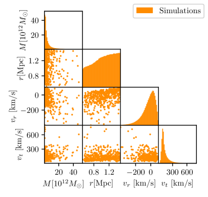
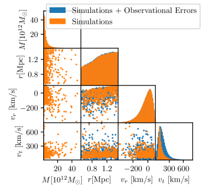
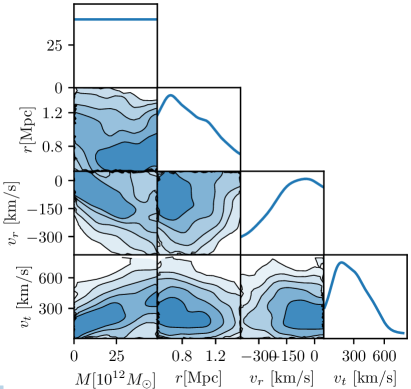
Having discussed the method, the simulations, and the data, we have everything we need to perform LFI using DELFI. We have three data points $d=\left\{r,v_{r},v_{t}\right\}$ and one parameter $\theta=M$. The process is illustrated in Fig. 2 and Fig. 3, and consists of the following:

1. Left panel of Fig. 2: We generate a large number of forward simulations, as discussed in Sec. IV. Increasing the number of simulations will increase the accuracy of the density estimation, and of the resulting posterior. Reference (Alsing et al., 2019) demonstrates an active learning scheme with pyDELFI, providing criteria to run new simulations based on discrepancies between the density estimates in the neural density estimator ensemble. However, due to our initial large number of simulations, we had no need to run such extra simulations on-the-fly.

2. Right panel of Fig. 2: The observational errors are introduced as scatter in the forward simulations. More specifically, we displace the simulations by a number sampled from the error model presented in Sec. V. Note how in Fig. 2 this step does not affect the mass. This is because the mass in this problem is part of the parameters $\theta$, not the data, as it is our goal to obtain a posterior distribution for the mass.

3. We use density estimation to get the conditional density distribution $p(d|\theta,I)$, as shown in Fig. 3. While it might seem counter-intuitive to learn the likelihood instead of directly learning the posterior, this allows us to then sample from a chosen prior, instead of being limited to the prior that is implicit in the simulations. This is discussed in more detail in Appendix A.

   There are several algorithms that can be used to get a conditional probability distribution from samples. In this work we use GMDN and MAF (as part of the pyDELFI package).

4. Finally, we evaluate this conditional density distribution at the observed data

   $$D_{\rm obs}=\{r=$0.77\text{\,}\mathrm{Mpc}$,\\ v_{r}=$-109.3\text{\,}\mathrm{km}\text{\,}{\mathrm{s}}^{-1}$,v_{t}=$72\text{\,}\mathrm{km}\text{\,}{\mathrm{s}}^{-1}$\},$$ (4)

   as discussed in Sec. V. This way, we get the likelihood function:

   $$\mathcal{L}\equiv p(d=D_{\rm obs}|\theta,I).$$ (5)

Through this process we obtain a likelihood function, without ever having to write a theory or use a Gaussian approximation. While this process is limited by the number and accuracy of the available simulations, it has a big advantage over likelihood-based problems that use simplifying approximations to make the likelihood more tractable, or easier to compute. The calculation of $M_{\rm MW+M31}$ is a good example: the likelihood-based approach relies on the TA and data modelling approximations, which we know oversimplifies the problem. Instead, using DELFI, we can account for the complex nonlinear evolution of the system through our N-body simulation.

VI.2 Density estimation validation

For the density estimation, with pyDELFI we use a combination of two GMDNs (with four and five Gaussian components) and two MAFs (with three and four components). The GMDNs have two layers with fifty components each, while the MAFs have thirty components on each of the two hidden layers. For a more robust density estimation we stack the results weighted by each density estimation’s relative likelihood, as described in (Alsing et al., 2019).

Figure 4: Validation plot for our density estimation. We use 10,000 simulations that have not be used for training. For all these, we use $r$, $v_{r}$ and $v_{t}$ to estimate a mass, and compare with the true mass. The top figure plots predicted vs true mass, while the bottom plot shows the residuals. The bars show the 68 % CL obtained using the method described in this paper.

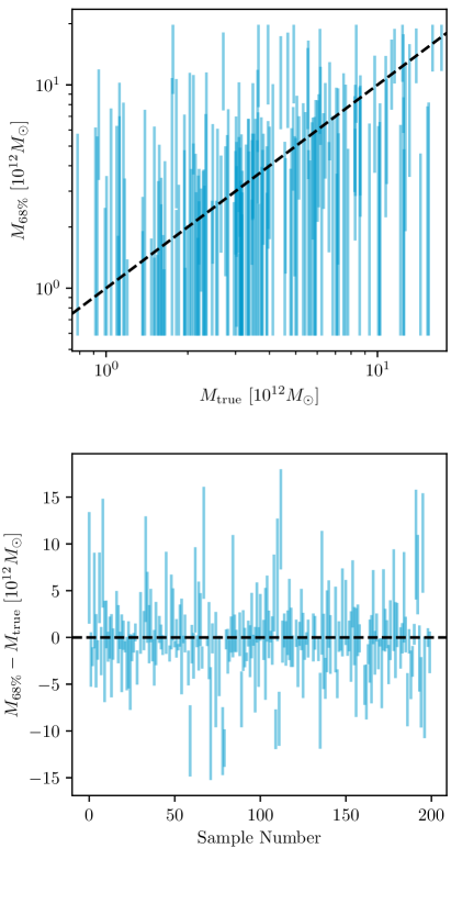
We hold back 10,000 simulations from the training set to be used for validating the likelihood that we have learned through the simulations. Each validation simulation has a ‘true’ mass, position and velocity, and we can use these to estimate how well our likelihood works. The results from this validation are shown in Fig. 4. We also perform a quartile test, finding that $95.485\%$ of the simulations fall within the $2\sigma$ predicted posterior, as expected.

VI.3 Prior distribution

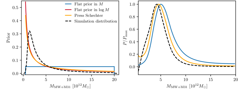
As previously discussed, we have the freedom to choose a suitable prior distribution (this is because we have used the simulations to learn a likelihood function, instead of directly learning the posterior distribution). The left panel of Fig. 8 shows four priors relevant to this study. Uninformative priors in this case could be either a flat prior or a logarithmic prior. In addition, in this problem Press-Schechter theory Press and Schechter (1974) supplies us with a physically-motivated prior. The Press-Schechter formalism predicts the number of virialized objects with a given mass. While this would be a fully correct prior only if the MW and M31 formed a single halo, it can provide a good prior distribution for the problem. We calculate the Press-Schechter prior using the code Colossus (Diemer, 2018), and the Tinker mass function (Tinker et al., 2008). Finally, the prior shown as a black dashed line is the one that would have been in use if we have learned the posterior directly from the simulations (when learning the posterior directly, we still have a prior, we simply lose the freedom to choose it). In this work, we adopt the Press-Schechter prior, which as shown in Fig. 8 is virtually equivalent to a flat prior in $\log M$. The effect of using different priors in our results will be discussed in Appendix B.

Once we have obtained a likelihood function and prior, we can get a posterior using Bayes’ theorem Eq. 2. We can describe this posterior by sampling from it using an algorithm such as Markov chain Monte Carlo (MCMC) or Nested Sampling (Skilling, ). However, in our case, a ‘brute-force’ approach is more practical (because the posterior is only one-dimensional): we simply calculate the posterior on a grid of mass values.

Our result using the Press-Schechter prior is shown in Fig. 5 (solid blue). Our peak and $68\%$ confidence levels are $M_{\rm MW+M31}=$ $4.6^{+2.3}_{-1.8}\times 10^{12}\text{\,}\mathrm{\mathit{M_{\odot}}}$, in good agreement with (McLeod et al., 2017) (also shown in Fig. 5) but with improved error bars.

VI.4 Results discussion

Figure 5: The posterior on $M_{\rm MW+M31}$ obtained in this work (solid blue) compared to the timing argument result of (McLeod et al., 2017) that includes $\Lambda$ and the tangential velocity from (van der Marel et al., 2019) (dashed orange). While our peak is lower, the posteriors are fully consistent.

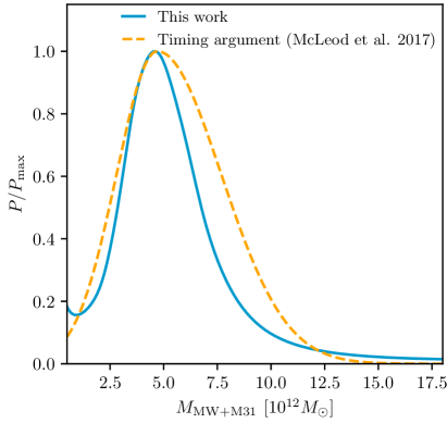
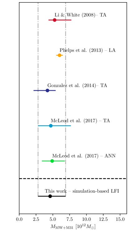
Our result is compared to previous results in Fig. 7. We see that all other estimates considered in this work are within the $68\%$ confidence interval of our posterior in the mass, despite the different methods used. We notice that the Least Action result of (Phelps et al., 2013)) obtains tighter constraints than our method; however, our result is the first one to fully account for the distribution of the observed errors in a robust (and Bayesian) manner. Other results use Gaussian approximations for observational errors, or neglect them completely, and therefore our result is the most accurate estimate of $M_{\rm MW+M31}$ to date. This framework also allows for more accurate estimates, in particular accounting for the presence of M33 and the LMC in the local group. This will be explored in future work.

The simulation was run using one particular set of cosmological parameters but in reality these parameters are uncertain and we should marginalise over them. This is infeasible for us, as we have a pre-run set of simulations with fixed cosmological parameters, but we can estimate the size of the effect by reference to the timing argument (TA).

The TA uses the same observational constraints as does this work, and like this work is based on modelling/simulating the trajectories of galaxies similar to those in the MW+M31 system; as a result the TA should have similar sensitivities to cosmological parameters as this work. The TA sensitivities can be estimated by numerically differentiating the mass estimation algorithm described in Partridge et al. (2013). We parameterise this algorithm using $h$ and $\Omega_{\Lambda}$ (from which $\Lambda$ and the age of the universe may be derived, the latter assuming $\Omega_{m}+\Omega_{\Lambda}=1$). We find $\partial M_{\rm MW+M31}/\partial\Omega_{\Lambda}=$-2.4\text{\times}{10}^{12}\text{\,}\mathrm{\mathit{M_{\odot}}}$$ and $\partial M_{\rm MW+M31}/\partial h=$7.4\text{\times}{10}^{12}\text{\,}\mathrm{\mathit{M_{\odot}}}$$. Multiplying these sensitivities by uncertainties on cosmological parameters ($\Delta\Omega_{\Lambda}=0.006$ and $\Delta h=0.004$ Planck Collaboration (2020)) yields uncertainties on the mass estimate that are immaterial compared to the uncertainty implied by the posterior width, and hence will be ignored. This conclusion continues to hold even if we assume a larger uncertainty on $h$ reflecting the current tension between early- and late-Universe measurements of this parameter. For example, a change in $h$ of $0.066\text{\,}\mathrm{i}$nduces a change in the TA $M_{\rm MW+M31}$ of $0.49\text{\times}{10}^{12}\text{\,}\mathrm{\mathit{M_{\odot}}}$ (in agreement with (McLeod and Lahav, 2019)); adding this in quadrature to the uncertainty implied by the posterior width yields only a marginal increase in total uncertainty (from $2.3\text{\times}{10}^{12}\text{\,}\mathrm{\mathit{M_{\odot}}}$ to $2.35\text{\times}{10}^{12}\text{\,}\mathrm{\mathit{M_{\odot}}}$). This calculation illustrates that in a simulation-based approach it is important to have a benchmark analytical model, to gauge if parameters not explored by the simulations are relevant and if extra simulations are needed.

Figure 6: A comparison of the estimates of the separate masses of M31, the MW, and their sum, the latter from this work. The plot shows the small discrepancy between separate estimates of the individual masses of the MW and M31 and this work.

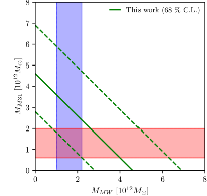
Finally, we can compare our results with separate estimates of the masses of the Milky Way and M31. There are several values in the literature for the separate masses of each galaxy, in some cases discrepant. Given this discrepancy, we take a number of estimates of each mass obtained through different methods, and assume that the true value is contained within the ranges of the different estimates, as done in Libeskind et al. (2020). While conservative, this method should provide with ranges that contain the true mass of each galaxy, and allow us to combine estimates in tension. Through this method, we get the following:

• $M_{\rm MW}\in(1.0,2.2)$ $\text{\,}\times\mathrm{1}\mathrm{0}^{12}\mathrm{\mathit{M_{\odot}}}$, from (Diaz et al., 2014; Zaritsky and Courtois, 2017; Hattori et al., 2018; Posti and Helmi, 2019; Watkins et al., 2019; Karukes et al., 2020)

• $M_{\rm M31}\in(0.6,2.0)$ $\text{\,}\times\mathrm{1}\mathrm{0}^{12}\mathrm{\mathit{M_{\odot}}}$, from (Corbelli et al., 2010; Tamm et al., 2012; Diaz et al., 2014; Kafle et al., 2018)

Combining these two measurements yields $M_{\rm MW+M31}\in(1.6,4.2)$ $\text{\,}\times\mathrm{1}\mathrm{0}^{12}\mathrm{\mathit{M_{\odot}}}$. This is slightly lower than our result, but still in agreement, as illustrated in Fig. 6. We can see in Fig. 7 that all estimates of the sum of the masses based on the relative distance and velocity of the bodies (TA, ANN and our approach) obtain slightly larger values than the sum of the separate masses. A possible explanation for this could be the fact that all these approaches ignore the effect of other bodies such as the LMC and M33 in the observed velocities, which could bias the sum of the masses to higher values (Peñarrubia et al., 2016). The effect of the LMC and M33 in our posterior mass will be explored in future work.

Figure 7: Comparison of this work with previous estimates of the $M_{\rm MW+M31}$, shown as best fit and $68\%$ confidence intervals. The result of this work is shown at the bottom; it is the first to account fully for the observational errors, and to not rely on the approximation of the TA.

VII Conclusions

In this work we have used Density Estimation Likelihood-Free Inference with forward-modelling to estimate the posterior distribution for sum of the masses of the Milky Way and M31 using observations of the distance and velocity to M31. We obtain a mass $M_{\rm MW+M31}=$ $4.6^{+2.3}_{-1.8}\times 10^{12}\text{\,}\mathrm{\mathit{M_{\odot}}}$ ($M_{200}$). Our method overcomes the several approximations of the traditional Timing Argument, accounts for non-Gaussian sources of observational measurement error, and uses a physically motivated prior; this makes it the most reliable estimate of $M_{\rm MW+M31}$ mass to date.

The sensitivity analysis performed in this study illustrates that in any simulation-based approach it is important to have a benchmark analytical (or semi-analytical) model, to assess how to cover the parameter space of required simulations.

This works serves not only to obtain state-of-the-art estimates of the $M_{\rm MW+M31}$; by applying Likelihood-Free Inference to a problem that is physically rich and complex yet statistically simple (thanks to its low dimensionality), we can illustrate how the method works, what different choices need to be made, and what challenges need to be tackled. The ability to robustly infer $M_{\rm MW+M31}$ without requiring an analytic theory or a likelihood demonstrates the potential of Likelihood-Free Inference methods in astronomy and cosmology.

Appendix A Density Estimators

Figure 8: On the left, a comparison of four possible priors: a flat prior in the mass (blue), a flat prior in the logarithm of the mass (red), a physically motivated Press-Schechter prior (orange), and the prior from the distribution of the simulations (dashed black). On the right, the corresponding posterior obtained from each prior. Note that we did not show the posterior for the flat prior in the logarithm of the mass, as this is equivalent to the Press-Schechter prior.

One of the key elements of DELFI is the estimation of a probability distribution from samples. This corresponds to going from Fig. 2 (right panel) to Fig. 3. The density estimation problem arises in many fields (for example image analysis (Theis and Bethge, 2015; Salimans et al., 2017)) and several algorithms have been developed to address it. In this section, we review some of the most popular density estimation methods in the context of LFI. For an overview of neural density estimation in the context of LFI we recommend Alsing et al. (2019).

Density estimation algorithms that rely on there being samples near the point of interest, such as spline or Kernel Density Estimation (KDE), struggle in high dimensional spaces due to the sparsity of the sampling. They are very useful, however, for estimating low dimensional PDFs, which is why they are often used for plotting marginalised posterior distributions. Public codes such as GetDist (Lewis, 2019), ChainConsumer (Hinton, 2016) or anesthetic (Handley, 2019) use KDE to generate plots of marginalised posterior distributions.

A Mixture Model (MM) represents a PDF $p$ as a weighted sum of component distributions:

$$p(\mathbf{y})=\sum_{c=1}^{N}\alpha_{c}\mathcal{D}(\mathbf{y};\Phi_{c}).$$ (6)

Here $N$ is the number of components in the mixture while $\mathcal{D}$ is some family of distributions described by parameters $\Phi$; the weights $\left\{\alpha_{c}\right\}$ and parameters $\left\{\Phi_{c}\right\}$ are fit to observed or training data. A common choice is the Gaussian Mixture Model (GMM), in which each component distribution is Gaussian: $\mathcal{D}(\mathbf{y};\Phi_{c})=\mathcal{N}(\mathbf{y};\mu_{c},\sigma_{c})$.

GMMs can successfully represent a large number of PDFs. In addition, they have the advantage that the weights and parameters $\left\{\alpha_{c},\mu_{c},\sigma_{c}\right\}$ can be easily fit to the data using the Expectation-Maximization algorithm (Dempster et al., 1977). There are, however, some issues with GMMs: they are sensitive to the choice of $N$, and they have problems fitting certain features (such as the sharp edges that can arise when flat priors are used).

In the context of LFI we are interested in modelling a conditional distribution $p(\mathbf{y}|\mathbf{x})$ (for example in our case $p$ is the conditional likelihood, for which $\mathbf{y}=d$ and $\mathbf{x}=\theta$). Such conditional distributions can be modelled by Mixture Density Networks (MDNs) (Bishop, 1994, 2006). As with MMs, they model the PDF as a weighted sum of component distributions, but now the weights and parameters describing the components are themselves (possibly non-linear) functions of $\mathbf{x}$:

$$p(\mathbf{y}|\mathbf{x})=\sum_{c=1}^{N}\mathbf{\alpha}_{c}(\mathbf{x})\mathcal{D}_{c}(\mathbf{y};\Phi_{c}(\mathbf{x})).$$ (7)

Again, a common choice is the Gaussian MDN (GMDN), in which each component is Gaussian: $\mathcal{D}(\mathbf{y};\Phi_{c}(\mathbf{x}))=\mathcal{N}(\mathbf{y};\mu_{c}(\mathbf{x}),\sigma_{c}(\mathbf{x}))$.

The functions $\left\{\mathbf{\alpha}_{c}(\mathbf{x}),\mu_{c}(\mathbf{x}),\sigma_{c}(\mathbf{x})\right\}$ can be modelled by a neural network with a set of weights; these weights are then fit to the data. As with GMMs, GMDNs require specification of the number $N$ of mixture components to be used; however, this dependence is much smaller than in the case of GMMs (as GMDNs can fit complex distributions using only a small number of components).

We finish by describing Masked Autoregressive Flows (MAFs), which have recently emerged as a powerful density estimation method (Papamakarios et al., 2017, 2019). They do not rely on a choice of number of components, and have the advantage of providing simple tests of the goodness of fit to the samples.

Here is the motivation for masking as a strategy for density estimation. Consider training a neural network NN to mimic; one can imagine training a parrot, for example. The trainer speaks (= input signal), and rewards the bird if its output matches this training input. If NN has sufficient complexity then it will learn to mimic the input. Now repeat the process but with a bird with covered (= masked) ears. The bird can’t hear the input, but nevertheless receives the training reward if its output matches the input. Now the bird can only ‘play the percentages’; it learns the optimal strategy, which is to output a weighted average of the input signals (weighted by their frequency of usage by the trainer). In this way the masked parrot learns the probability distribution of the input signal i.e. has become a density estimator.

That was the one-dimensional case. The two dimensional case needs two parrots. The first is trained on signal $x_{1}$, which it can’t hear, with the result that it learns $p(x_{1})$. The second is trained on $x_{2}$, which it can’t hear, but it is allowed to hear $x_{1}$. As a result it learns $p(x_{2}|x_{1})$. Thus between them they learn $p(x_{1})p(x_{2}|x_{1})=p(x_{1},x_{2})$ as desired. The multi-dimensional case is similar. This strategy is called an autoregressive autoencoder. Note that it treats the coordinates asymmetrically.

The conditional distributions $p(x_{i}|x_{1},\dots,x_{i-1})$ learned by NN are typically modelled as Gaussian. Consider generating samples from the estimated probability distribution $p$; for each sample we need we a set of $n$ random unit normals (i.e. a draw from $N(0,I)$), which we transform to get samples from $p$ - call this transform $T$. The details of $T$ come from the means and standard deviations of the conditional distributions, which can be obtained from $n$ evaluations of NN. However, importantly, the inverse mapping $T^{-1}$ can be found with just one evaluation of NN. This is the idea of the Masked Autoencoder for Distribution Estimation (MADE) algorithm (Germain et al., 2015).

Now apply $T^{-1}$ to the training data $D$. The resulting ‘pulled-back’ data $T^{-1}(D)$ will ideally be a set of samples from $N(0,I)$ and its deviation from this ideal gives a direct measure of how imperfect is our modelling of $p$. We can then use the ‘pulled-back’ data as the training data for yet another MADE process, and so on through several iterations. Between iterations we permute the coordinate axes, thereby symmetrising how we treat them. With sufficient iterations, the multiply-pulled-back training data approaches $N(0,I)$; at this point the algorithm has an easy-to-evaluate mapping between $p$ and $N(0,I)$, which suffices for doing calculations. This is the Masked Autoregressive Flows (MAF) algorithm (Papamakarios et al., 2017, 2019).

Appendix B Dependence on Priors

In this appendix, we explore how the posterior distribution of $M_{\rm MW+M31}$ (as shown in Fig. 5 and discussed in Sec. VI) depends on our choice of prior. We consider the four different priors illustrated in Fig. 8:

• A flat prior in the mass;

• A logarithmic prior in the mass;

• A prior based on the Press-Schechter distribution (as adopted in this work);

• A prior distribution matching the distribution of masses in the simulation.

In our case the second and third choices are virtually the same (as shown in the left panel of Fig. 8), and so we omit the ‘logarithmic in mass’ prior when examining how the priors affect our results. The posteriors obtained when using the remaining three priors are shown in the right panel of Fig. 8, and we see that our result is essentially independent of our choice of prior, be it the Press-Schechter prior, a flat prior on the mass ($M_{\rm LG}(\textrm{Flat prior})=5.0^{+2.7}_{-1.7}\times 10^{12}M_{\odot}$) or the prior from the simulation distribution. ($M_{\rm LG}(\textrm{Simulation Distribution})=4.3\pm 1.7\times 10^{12}M_{\odot}$)

Appendix C Dependence on Tangential Velocity

Figure 9: The posterior on $M_{\rm MW+M31}$ for different values of the tangential velocity: $v_{t}=$ $72\text{\,}\mathrm{km}\text{\,}{\mathrm{s}}^{-1}$ as used in this work (solid blue), and a purely radial motion $v_{t}=0$ (dashed red).

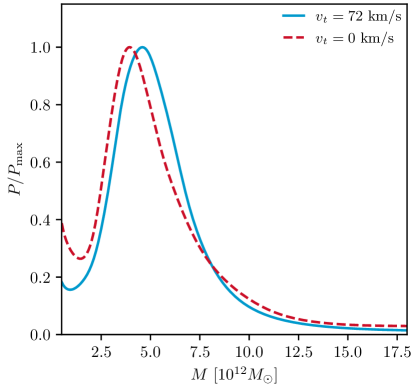
Imagine a 2-dimensional velocity vector ${\bf V}=(V_{x},V_{y})$. If $V_{x},V_{y}$ are uncorrelated, normally distributed with zero mean and equal variance $\sigma$, then the overall speed $V={\sqrt{(V_{x}^{2}+V_{y}^{2})}}$ will be characterized by the Rayleigh distribution (Rayleigh, 1905), with mean ${\bar{V}}=\sigma\sqrt{\pi/2}$, rather than naively zero. Similarly, non-zero measurements of ${V_{x},V_{y}}$ with error bars will result in a distribution function with a mean that is not ${\bar{V}}={\sqrt{(V_{x}^{2}+V_{y}^{2})}}$. In our analysis we pay attention to this via the forward modeling approach, starting with simulated $(V_{x},V_{y})$ and propagating their impact on the final posterior for $M_{\rm MW+M31}$.

While distance and radial velocity have been measured in numerous occasions using different methods, observations of the tangential velocity are far more scarce (van der Marel and Guhathakurta, 2008; van der Marel et al., 2012, 2019). Their work treats the effect of converting measurements of two components of the tangential velocity into a modulus in a novel way. We check the robustness of our approach in this section. We do so by comparing the main result of the paper to the case of no tangential velocity. As shown in Fig. 9, our posterior on the mass does not depend strongly on the tangential velocity. Therefore, we are confident on the accuracy of our posterior in the mass.

References

- Leclercq [2018] Florent Leclercq. Bayesian optimization for likelihood-free cosmological inference. Phys. Rev. D, 98(6):063511, September 2018. doi: 10.1103/PhysRevD.98.063511.
- Alsing et al. [2019] Justin Alsing, Tom Charnock, Stephen Feeney, and Benjamin Wand elt. Fast likelihood-free cosmology with neural density estimators and active learning. MNRAS, 488(3):4440–4458, September 2019. doi: 10.1093/mnras/stz1960.
- Betoule et al. [2014] M. Betoule, R. Kessler, J. Guy, J. Mosher, and D. Hardin et al. Improved cosmological constraints from a joint analysis of the SDSS-II and SNLS supernova samples. A&A, 568:A22, August 2014. doi: 10.1051/0004-6361/201423413.
- Wang et al. [2020] Yu-Chen Wang, Yuan-Bo Xie, Tong-Jie Zhang, Hui-Chao Huang, Tingting Zhang, and Kun Liu. Likelihood-free Cosmological Constraints with Artificial Neural Networks: An Application on Hubble Parameters and SN Ia. arXiv e-prints, art. arXiv:2005.10628, May 2020.
- Jeffrey et al. [2020] Niall Jeffrey, Justin Alsing, and Francois Lanusse. Likelihood-free inference with neural compression of DES SV weak lensing map statistics. arXiv e-prints, art. arXiv:2009.08459, September 2020.
- Brehmer et al. [2019] Johann Brehmer, Siddharth Mishra-Sharma, Joeri Hermans, Gilles Louppe, and Kyle Cranmer. Mining for Dark Matter Substructure: Inferring subhalo population properties from strong lenses with machine learning. 9 2019. doi: 10.3847/1538-4357/ab4c41.
- Ramanah et al. [2020] Doogesh Kodi Ramanah, Radosław Wojtak, and Nikki Arendse. Simulation-based inference of dynamical galaxy cluster masses with 3D convolutional neural networks. 9 2020.
- Tortorelli et al. [2020] Luca Tortorelli, Martina Fagioli, Jörg Herbel, Adam Amara, Tomasz Kacprzak, and Alexandre Refregier. Measurement of the B-band galaxy Luminosity Function with Approximate Bayesian Computation. J. Cosmology Astropart. Phys, 2020(9):048, September 2020. doi: 10.1088/1475-7516/2020/09/048.
- Kahn and Woltjer [1959] F. D. Kahn and L. Woltjer. Intergalactic Matter and the Galaxy. ApJ, 130:705, November 1959. doi: 10.1086/146762.
- Prada et al. [2012] Francisco Prada, Anatoly A. Klypin, Antonio J. Cuesta, Juan E. Betancort-Rijo, and Joel Primack. Halo concentrations in the standard cold dark matter cosmology. MNRAS, 423(4):3018–3030, July 2012. doi: 10.1111/j.1365-2966.2012.21007.x.
- Riebe et al. [2013] K. Riebe, A. M. Partl, H. Enke, J. Forero-Romero, S. Gottlöber, A. Klypin, G. Lemson, F. Prada, J. R. Primack, M. Steinmetz, and V. Turchaninov. The MultiDark Database: Release of the Bolshoi and MultiDark cosmological simulations. Astronomische Nachrichten, 334(7):691–708, August 2013. doi: 10.1002/asna.201211900.
- Meylan et al. [2004] Georges Meylan, Juan P. Madrid, and Duccio Macchetto. Hubble Space Telescope Science Metrics. PASP, 116(822):790–796, August 2004. doi: 10.1086/423227.
- Gaia Collaboration [2016] Gaia Collaboration. The Gaia mission. A&A, 595:A1, November 2016. doi: 10.1051/0004-6361/201629272.
- McLeod et al. [2017] M. McLeod, N. Libeskind, O. Lahav, and Y. Hoffman. Estimating the mass of the Local Group using machine learning applied to numerical simulations. J. Cosmology Astropart. Phys, 2017(12):034, December 2017. doi: 10.1088/1475-7516/2017/12/034.
- Bonassi et al. [2011] F.V. Bonassi, L. You, and M. West. Bayesian Learning from Marginal Data in Bionetwork Models. Statistical applications in genetics and molecular biology, 2011(10,1):49, October 2011. doi: 10.2202/1544-6115.1684.
- Fan et al. [2012] Y. Fan, D. J. Nott, and S. A. Sisson. Approximate Bayesian Computation via Regression Density Estimation. arXiv e-prints, art. arXiv:1212.1479, December 2012.
- Papamakarios and Murray [2016] George Papamakarios and Iain Murray. Fast -free Inference of Simulation Models with Bayesian Conditional Density Estimation. arXiv e-prints, art. arXiv:1605.06376, May 2016.
- Li and White [2008] Yang-Shyang Li and Simon D.M. White. Masses for the Local Group and the Milky Way. Mon. Not. Roy. Astron. Soc., 384:1459–1468, 2008. doi: 10.1111/j.1365-2966.2007.12748.x.
- Gonzalez et al. [2014] Roberto E. Gonzalez, Andrey V. Kravtsov, and Nickolay Y. Gnedin. On the mass of the Local Group. Astrophys. J., 793:91, 2014. doi: 10.1088/0004-637X/793/2/91.
- Phelps et al. [2013] Steven Phelps, Adi Nusser, and Vincent Desjacques. The mass of the Milky Way and M31 using the method of least action. Astrophys. J., 775:102, 2013. doi: 10.1088/0004-637X/775/2/102.
- Lynden-Bell [1981] D. Lynden-Bell. The dynamical age of the local group of galaxies. The Observatory, 101:111–114, August 1981.
- Binney and Tremaine [1987] James Binney and Scott Tremaine. Galactic dynamics. 1987.
- Partridge et al. [2013] Candace Partridge, Ofer Lahav, and Yehuda Hoffman. Weighing the Local Group in the Presence of Dark Energy. Mon. Not. Roy. Astron. Soc., 436:45, 2013. doi: 10.1093/mnrasl/slt109.
- McLeod and Lahav [2019] Michael McLeod and Ofer Lahav. The Two Body Problem in the Presence of Dark Energy and Modified Gravity: Application to the Local Group. arXiv e-prints, art. arXiv:1903.10849, March 2019.
- Benisty et al. [2019] David Benisty, Eduardo I. Guendelman, and Ofer Lahav. Milky Way and Andromeda past-encounters in different gravity models: the impact on the estimated Local Group mass. arXiv e-prints, art. arXiv:1904.03153, April 2019.
- Peebles [1994] P. J. E. Peebles. Orbits of the Nearby Galaxies. ApJ, 429:43, July 1994. doi: 10.1086/174301.
- Rubin [1984] Donald B Rubin. Bayesianly justifiable and relevant frequency calculations for the applied statistician. The Annals of Statistics, pages 1151–1172, 1984.
- [28] Murray Rosenblatt. Remarks on some nonparametric estimates of a density function. Ann. Math. Statist., (3):832–837, 09 . doi: 10.1214/aoms/1177728190.
- [29] Emanuel Parzen. On estimation of a probability density function and mode. Ann. Math. Statist., (3):1065–1076, 09 . doi: 10.1214/aoms/1177704472.
- Simonoff [1996] J.S. Simonoff. Smoothing Methods in Statistics. Springer Series in Statistics. Springer, 1996. ISBN 9780387947167. URL https://books.google.co.uk/books?id=wFTgNXL4feIC.
- Bishop [1994] Christopher M. Bishop. Mixture density networks. Technical report, 1994.
- Bishop [2006] Christopher M. Bishop. Pattern Recognition and Machine Learning (Information Science and Statistics). Springer-Verlag, Berlin, Heidelberg, 2006. ISBN 0387310738.
- Papamakarios et al. [2017] George Papamakarios, Theo Pavlakou, and Iain Murray. Masked autoregressive flow for density estimation. In Advances in Neural Information Processing Systems, pages 2338–2347, 2017.
- Cameron and Pettitt [2012] E. Cameron and A. N. Pettitt. Approximate Bayesian Computation for astronomical model analysis: a case study in galaxy demographics and morphological transformation at high redshift. MNRAS, 425(1):44–65, September 2012. doi: 10.1111/j.1365-2966.2012.21371.x.
- Weyant et al. [2013] Anja Weyant, Chad Schafer, and W. Michael Wood-Vasey. Likelihood-free Cosmological Inference with Type Ia Supernovae: Approximate Bayesian Computation for a Complete Treatment of Uncertainty. ApJ, 764(2):116, February 2013. doi: 10.1088/0004-637X/764/2/116.
- Akeret et al. [2015] Joël Akeret, Alexandre Refregier, Adam Amara, Sebastian Seehars, and Caspar Hasner. Approximate Bayesian Computation for Forward Modeling in Cosmology. JCAP, 08:043, 2015. doi: 10.1088/1475-7516/2015/08/043.
- Hahn et al. [2017] ChangHoon Hahn, Mohammadjavad Vakili, Kilian Walsh, Andrew P. Hearin, David W. Hogg, and Duncan Campbell. Approximate Bayesian computation in large-scale structure: constraining the galaxy–halo connection. Mon. Not. Roy. Astron. Soc., 469(3):2791–2805, 2017. doi: 10.1093/mnras/stx894.
- Peel et al. [2017] Austin Peel, Chieh-An Lin, Francois Lanusse, Adrienne Leonard, Jean-Luc Starck, and Martin Kilbinger. Cosmological constraints with weak lensing peak counts and second-order statistics in a large-field survey. Astron. Astrophys., 599:A79, 2017. doi: 10.1051/0004-6361/201629928.
- Kacprzak et al. [2018] T. Kacprzak, J. Herbel, A. Amara, and A. Réfrégier. Accelerating Approximate Bayesian Computation with Quantile Regression: application to cosmological redshift distributions. JCAP, 02:042, 2018. doi: 10.1088/1475-7516/2018/02/042.
- Alsing et al. [2018] Justin Alsing, Benjamin Wandelt, and Stephen Feeney. Massive optimal data compression and density estimation for scalable, likelihood-free inference in cosmology. MNRAS, 477(3):2874–2885, July 2018. doi: 10.1093/mnras/sty819.
- Alsing and Wandelt [2018] Justin Alsing and Benjamin Wandelt. Generalized massive optimal data compression. MNRAS, 476(1):L60–L64, May 2018. doi: 10.1093/mnrasl/sly029.
- Heavens et al. [2020] Alan F Heavens, Elena Sellentin, and Andrew H Jaffe. Extreme data compression while searching for new physics. Monthly Notices of the Royal Astronomical Society, 498(3):3440–3451, 2020.
- Papamakarios et al. [2019] George Papamakarios, David Sterratt, and Iain Murray. Sequential neural likelihood: Fast likelihood-free inference with autoregressive flows. In The 22nd International Conference on Artificial Intelligence and Statistics, pages 837–848. PMLR, 2019.
- Lueckmann et al. [2019] Jan-Matthis Lueckmann, Giacomo Bassetto, Theofanis Karaletsos, and Jakob H Macke. Likelihood-free inference with emulator networks. In Symposium on Advances in Approximate Bayesian Inference, pages 32–53. PMLR, 2019.
- Knebe et al. [2011] Alexander Knebe, Steffen R. Knollmann, Stuart I. Muldrew, Frazer R. Pearce, and Miguel Angel Aragon-Calvo et al. Haloes gone MAD: The Halo-Finder Comparison Project. MNRAS, 415(3):2293–2318, August 2011. doi: 10.1111/j.1365-2966.2011.18858.x.
- Holland [1998] Stephen Holland. The Distance to the M31 Globular Cluster System. Astron. J., 115:1916, 1998. doi: 10.1086/300348.
- Joshi et al. [2003] Y.C. Joshi, A.K. Pandey, D. Narasimha, R. Sagar, and Y. Giraud-Hiraud. Identification of 13 Cepheids and 333 other variables in M 31. Astron. Astrophys., 402:113–123, 2003. doi: 10.1051/0004-6361:20030136.
- Ribas et al. [2005] Ignasi Ribas, Carme Jordi, Francesc Vilardell, Edward L. Fitzpatrick, Ron W. Hilditch, and Edward F. Guinan. First determination of the distance and fundamental properties of an eclipsing binary in the andromeda galaxy. Astrophys. J. Lett., 635:L37–L40, 2005. doi: 10.1086/499161.
- McConnachie and Irwin [2006] Alan McConnachie and Mike Irwin. Structural parameters for the m31 dwarf spheroidals. Mon. Not. Roy. Astron. Soc., 365:1263, 2006. doi: 10.1111/j.1365-2966.2005.09806.x.
- van der Marel et al. [2019] Roeland P. van der Marel, Mark A. Fardal, Sangmo Tony Sohn, Ekta Patel, Gurtina Besla, Andrés del Pino, Johannes Sahlmann, and Laura L. Watkins. First Gaia Dynamics of the Andromeda System: DR2 Proper Motions, Orbits, and Rotation of M31 and M33. ApJ, 872(1):24, February 2019. doi: 10.3847/1538-4357/ab001b.
- van der Marel et al. [2012] Roeland P. van der Marel, Gurtina Besla, T. J. Cox, Sangmo Tony Sohn, and Jay Anderson. The M31 Velocity Vector. III. Future Milky Way M31-M33 Orbital Evolution, Merging, and Fate of the Sun. ApJ, 753(1):9, July 2012. doi: 10.1088/0004-637X/753/1/9.
- van der Marel and Guhathakurta [2008] Roeland P. van der Marel and Puragra Guhathakurta. M31 Transverse Velocity and Local Group Mass from Satellite Kinematics. Astrophys. J., 678:187, 2008. doi: 10.1086/533430.
- Skilling et al. [2006] John Skilling et al. Nested sampling for general bayesian computation. Bayesian analysis, 1(4):833–859, 2006.
- Handley et al. [2015a] W. J. Handley, M. P. Hobson, and A. N. Lasenby. POLYCHORD: nested sampling for cosmology. MNRAS, 450:L61–L65, June 2015a. doi: 10.1093/mnrasl/slv047.
- Handley et al. [2015b] W. J. Handley, M. P. Hobson, and A. N. Lasenby. POLYCHORD: next-generation nested sampling. MNRAS, 453:4384–4398, November 2015b. doi: 10.1093/mnras/stv1911.
- Handley [2019] Will Handley. anesthetic: nested sampling visualisation. The Journal of Open Source Software, 4(37):1414, Jun 2019. doi: 10.21105/joss.01414.
- O’Brien et al. [2016] Travis O’Brien, Karthik Kashinath, Nicholas Cavanaugh, William Collins, and John O’Brien. A fast and objective multidimensional kernel density estimation method: Fastkde. Computational Statistics & Data Analysis, 101, 03 2016. doi: 10.1016/j.csda.2016.02.014.
- O’Brien et al. [2014] Travis O’Brien, William Collins, Sara Rauscher, and Todd Ringler. Reducing the computational cost of the ecf using a nufft: A fast and objective probability density estimation method. Computational Statistics & Data Analysis, 79, 11 2014. doi: 10.1016/j.csda.2014.06.002.
- Press and Schechter [1974] William H. Press and Paul Schechter. Formation of Galaxies and Clusters of Galaxies by Self-Similar Gravitational Condensation. ApJ, 187:425–438, February 1974. doi: 10.1086/152650.
- Diemer [2018] Benedikt Diemer. COLOSSUS: A python toolkit for cosmology, large-scale structure, and dark matter halos. Astrophys. J. Suppl., 239(2):35, 2018. doi: 10.3847/1538-4365/aaee8c.
- Tinker et al. [2008] Jeremy L. Tinker, Andrey V. Kravtsov, Anatoly Klypin, Kevork Abazajian, Michael S. Warren, Gustavo Yepes, Stefan Gottlober, and Daniel E. Holz. Toward a halo mass function for precision cosmology: The Limits of universality. Astrophys. J., 688:709–728, 2008. doi: 10.1086/591439.
- [62] John Skilling. Nested sampling for general bayesian computation. Bayesian Anal., (4):833–859, 12 . doi: 10.1214/06-BA127.
- Planck Collaboration [2020] Planck Collaboration. Planck 2018 results - vi. cosmological parameters. A&A, 641:A6, 2020. doi: 10.1051/0004-6361/201833910.
- Libeskind et al. [2020] Noam I. Libeskind, Edoardo Carlesi, Robert J. J. Grand, Arman Khalatyan, Alexander Knebe, Ruediger Pakmor, Sergey Pilipenko, Marcel S. Pawlowski, Martin Sparre, Elmo Tempel, Peng Wang, Hélène M. Courtois, Stefan Gottlöber, Yehuda Hoffman, Ivan Minchev, Christoph Pfrommer, Jenny G. Sorce, Volker Springel, Matthias Steinmetz, R. Brent Tully, Mark Vogelsberger, and Gustavo Yepes. The HESTIA project: simulations of the Local Group. MNRAS, 498(2):2968–2983, August 2020. doi: 10.1093/mnras/staa2541.
- Diaz et al. [2014] J. D. Diaz, S. E. Koposov, M. Irwin, V. Belokurov, and N. W. Evans. Balancing mass and momentum in the Local Group. MNRAS, 443(2):1688–1703, September 2014. doi: 10.1093/mnras/stu1210.
- Zaritsky and Courtois [2017] Dennis Zaritsky and Helene Courtois. A dynamics-free lower bound on the mass of our Galaxy. MNRAS, 465(3):3724–3728, March 2017. doi: 10.1093/mnras/stw2922.
- Hattori et al. [2018] Kohei Hattori, Monica Valluri, Eric F. Bell, and Ian U. Roederer. Old, Metal-Poor Extreme Velocity Stars in the Solar Neighborhood. Astrophys. J., 866(2):121, 2018. doi: 10.3847/1538-4357/aadee5.
- Posti and Helmi [2019] Lorenzo Posti and Amina Helmi. Mass and shape of the Milky Way’s dark matter halo with globular clusters from Gaia and Hubble. A&A, 621:A56, January 2019. doi: 10.1051/0004-6361/201833355.
- Watkins et al. [2019] Laura L. Watkins, Roeland P. van der Marel, Sangmo Tony Sohn, and N. Wyn Evans. Evidence for an Intermediate-mass Milky Way from Gaia DR2 Halo Globular Cluster Motions. ApJ, 873(2):118, March 2019. doi: 10.3847/1538-4357/ab089f.
- Karukes et al. [2020] Ekaterina V. Karukes, Maria Benito, Fabio Iocco, Roberto Trotta, and Alex Geringer-Sameth. A robust estimate of the Milky Way mass from rotation curve data. JCAP, 05:033, 2020. doi: 10.1088/1475-7516/2020/05/033.
- Corbelli et al. [2010] E. Corbelli, S. Lorenzoni, R. Walterbos, R. Braun, and D. Thilker. A wide-field H I mosaic of Messier 31. II. The disk warp, rotation, and the dark matter halo. A&A, 511:A89, February 2010. doi: 10.1051/0004-6361/200913297.
- Tamm et al. [2012] A. Tamm, E. Tempel, P. Tenjes, O. Tihhonova, and T. Tuvikene. Stellar mass map and dark matter distribution in M 31. A&A, 546:A4, October 2012. doi: 10.1051/0004-6361/201220065.
- Kafle et al. [2018] Prajwal R. Kafle, Sanjib Sharma, Geraint F. Lewis, Aaron S. G. Robotham, and Simon P. Driver. The Need for Speed: Escape velocity and dynamical mass measurements of the Andromeda galaxy. Mon. Not. Roy. Astron. Soc., 475(3):4043–4054, 2018. doi: 10.1093/mnras/sty082.
- Peñarrubia et al. [2016] Jorge Peñarrubia, Facundo A. Gómez, Gurtina Besla, Denis Erkal, and Yin-Zhe Ma. A timing constraint on the (total) mass of the Large Magellanic Cloud. MNRAS, 456(1):L54–L58, February 2016. doi: 10.1093/mnrasl/slv160.
- Theis and Bethge [2015] Lucas Theis and Matthias Bethge. Generative image modeling using spatial lstms. In Advances in Neural Information Processing Systems, pages 1927–1935, 2015.
- Salimans et al. [2017] Tim Salimans, Andrej Karpathy, Xi Chen, and Diederik P. Kingma. PixelCNN++: Improving the PixelCNN with Discretized Logistic Mixture Likelihood and Other Modifications. arXiv e-prints, art. arXiv:1701.05517, January 2017.
- Lewis [2019] Antony Lewis. GetDist: a Python package for analysing Monte Carlo samples. 2019. URL https://getdist.readthedocs.io.
- Hinton [2016] S. R. Hinton. ChainConsumer. The Journal of Open Source Software, 1:00045, August 2016. doi: 10.21105/joss.00045.
- Dempster et al. [1977] A. P. Dempster, N. M. Laird, and D. B. Rubin. Maximum likelihood from incomplete data via the em algorithm. Journal of the Royal Statistical Society. Series B (Methodological), 39(1):1–38, 1977. ISSN 00359246. URL http://www.jstor.org/stable/2984875.
- Germain et al. [2015] Mathieu Germain, Karol Gregor, Iain Murray, and Hugo Larochelle. Made: Masked autoencoder for distribution estimation. In International Conference on Machine Learning, pages 881–889, 2015.
- Rayleigh [1905] Lord Rayleigh. The problem of the random walk. Nature, 72(1866):318, 1905.