Towards Accurate Knowledge Transfer via Target-awareness Representation Disentanglement

Abstract

Fine-tuning deep neural networks pre-trained on large scale datasets is one of the most practical transfer learning paradigm given limited quantity of training samples. To obtain better generalization, using the starting point as the reference (SPAR), either through weights or features, has been successfully applied to transfer learning as a regularizer. However, due to the domain discrepancy between the source and target task, there exists obvious risk of negative transfer in a straightforward manner of knowledge preserving. In this paper, we propose a novel transfer learning algorithm, introducing the idea of Target-awareness REpresentation Disentanglement ($\mathrm{TRED}$), where the relevant knowledge with respect to the target task is disentangled from the original source model and used as a regularizer during fine-tuning the target model. Specifically, we design two alternative methods, maximizing the Maximum Mean Discrepancy (Max-MMD) and minimizing the mutual information (Min-MI), for the representation disentanglement. Experiments on various real world datasets show that our method stably improves the standard fine-tuning by more than 2% in average. $\mathrm{TRED}$ also outperforms related state-of-the-art transfer learning regularizers such as $\mathrm{L^{2}\text{-}SP}$, $\mathrm{AT}$, $\mathrm{DELTA}$, and $\mathrm{BSS}$.

I Introduction

Deep convolutional networks achieve great success on large scale vision tasks such as ImageNet [1] and Places365 [2]. In addition to their notable improvements of accuracy, deep representations learned on modern CNNs are demonstrated transferable across relevant tasks [3]. This is rather fortunate for many real world applications with inefficient labeled examples. Transfer learning aims to obtain good performance on such tasks by leveraging knowledge learned by relevant large scale datasets. The auxiliary and desired tasks are called the source and target tasks respectively. According to [4], we focus on inductive transfer learning, which cares about the situation that the source and target tasks have different label spaces.

The most popular practice is to fine-tune a model pre-trained on the source task with the $\mathrm{L^{2}}$ regularization, which has the effect of constraining the parameter around the origin of zeros. [5] points out that since the parameter may be driven far from the starting point of the pre-trained model, a major disadvantage of naive fine-tuning is the risk of catastrophic forgetting [6] of the knowledge learned from source. They recommend to use the $\mathrm{L^{2}\text{-}SP}$ regularizer instead of the popular $\mathrm{L^{2}}$. While in parallel, knowledge distillation, which is originally designed for compressing the knowledge in a complex model to a simple one [7], is proved to be useful for transfer learning tasks where knowledge is distilled from a different dataset [8, 9]. Recent work [10] formulates knowledge distillation in transfer learning as a regularizer on features and further improves through unactivated channel reusing for better fitting the training samples. These methods adopt a common assumption that, the relevant knowledge contained in the source model is expected to facilitate the generalization of the target model. This leads to the motivation of regularizing the fine-tuned model using the starting point as the reference (SPAR) in a mainstream group of inductive transfer learning algorithms [5, 8, 10].

Although the advanced methods with SPAR have succeed to preserve the knowledge contained in the source model, fine-tuning also takes the obvious risk of negative transfer [11]. Intuitively, if the source and target data distribution are dissimilar to some extent, not all the knowledge from the source is transferable to the target and an indiscriminate transfer could be detrimental to the target model. However, the impact of negative transfer has been rarely considered in inductive transfer learning studies. The most related work, [12], proposed to investigate the regularizer of Batch Spectral Shrinkage ($\mathrm{BSS}$) to inhibit negative transfer, where the small singular values of feature representations are considered as not transferable and suppressed. Yet, it is hard to adaptively determine the scope of small singular value when faced with different target tasks. Moreover, $\mathrm{BSS}$ does not take consideration of the catastrophic forgetting risk, which means it has to be equipped with other fine-tuning techniques (e.g., $\mathrm{L^{2}\text{-}SP}$ [5], Attention-Transfer [8], $\mathrm{DELTA}$ [10], etc.) to achieve considerable performance.

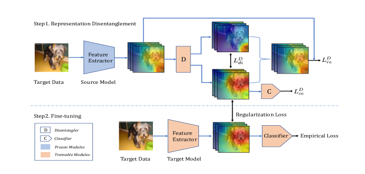
According to the above analysis, it is straightforward to think about a better solution which simultaneously takes the consideration of preserving relevant knowledge and avoiding negative transfer. In this paper, we intend to improve the standard fine-tuning paradigm by accurate knowledge transfer. Assuming that the knowledge contained in the source model consists of one part relevant to the target task and the other part which is irrelevant, we are going to explicitly disentangle the former from the source model. Thus, a target task specific starting point is used as the reference instead of the original one. Specifically, we design a novel regularizer of deep transfer learning through Target-awareness REpresentation Disentanglement ($\mathrm{TRED}$). The whole algorithm includes two steps. First we use a lightweight disentangler to separate middle representations of the pre-trained source model into the positive and negative parts. The core component of the disentangler is a differentiable module which is capable of separating the positive and negative group of features. We propose two alternative methods for the disentanglement, which are maximizing the Maximum Mean Discrepancy (Max-MMD) on the spatial dimension, and minimizing the Mutual Information (Min-MI) on the channel dimension. Intuitively, we intend to distill the relevant ingredients from noisy features by separating irrelevant ingredients which should: (1) pay attention to different regions with the the relevant ones; or (2) have independent semantic representations with the relevant ones. The disentanglement is achieved by simultaneously optimizing the disentangling module and ensuring to reconstruct the original representation. Supervision information from labeled target examples is utilized to distinguish the positive part from the negative part. The second step is to perform fine-tuning using the disentangled positive part of representations as the reference. In summary, our main contributions are as following:

• We are the first to involve the idea of representation disentanglement to improve inductive transfer learning.

• Our algorithm aiming at accurate knowledge transfer contributes to the study of negative transfer.

• Our proposed $\mathrm{TRED}$ significantly outperforms state-of-the-art transfer learning regularizers including $\mathrm{L^{2}}$, $\mathrm{L^{2}\text{-}SP}$, $\mathrm{AT}$, $\mathrm{DELTA}$ and $\mathrm{BSS}$ on various real world datasets.

[t] Comparison among different fine-tuning approaches. Approach Risk $Considered$ CF^* NT^* $\mathrm{L^{2}}$ [13]  ✗  ✗ SPAR [8, 5, 10]  ✓  ✗ BSS [12]  ✗  ✓ TRED  ✓  ✓

• CF=Catastrophic Forgetting, NT=Negative Transfer, SPAR=Starting Point As the Reference.

Figure 1: The architecture of deep transfer learning through Target-awareness Representation Disentanglement ($\mathrm{TRED}$).

II Related Work

II-A Shrinkage Towards Chosen Parameters

Regularization techniques have a long history since Stein’s paradox [14, 15], showing that shrinking towards chosen parameters obtains an estimate more accurate than simply using observed averages. Most common choices like Lasso and Ridge Regression pull the model towards zero, while it is widely believed that shrinking towards “true parameters” is more effective. In transfer learning, models pre-trained on relevant source tasks with sufficient labeled examples are often regarded as “true parameters”. Earlier works demonstrate its effectiveness on Maximum Entropy [16] or Support Vector Machine models [17, 18, 19].

Despite that the notion of “true parameters” of deep neural networks is intractable, several studies [20, 3, 21] have demonstrated the great transferability of representations trained on large scale datasets for general purpose.  [22] theoretically studies properties of the pre-traind model and explains why it outperforms training from scratch.

II-B Deep Inductive Transfer Learning

Despite the great transferability, recent work [5] points out that naive fine-tuning the pre-trained model with $\mathrm{L^{2}}$ regularization may cause losses of the original knowledge. In order to overcome over-fitting, various transfer learning regularizers have been proposed. According to the type of regularized objectives, they can be categorized as parameter based [5], feature based [8, 9, 10] or spectral based [12] methods.

[12] improves the regularization of transfer learning from another angle. They propose Batch Spectral Shrinkage (BSS) to regularize spectral components of deep representations by penalizing small singular values. BSS is complementary to other regularizers. However, it doesn’t deal with the issue of knowledge preserving.

Our paper adopts the general idea of preserving knowledge by regularizing features of the source model. While unlike previous methods, we do not directly use the original knowledge provided by the source model. Instead, we disentangle the useful part for reference to avoid negative transfer. There main differences are summarized in Table I.

Studies from other angles, such as sample selection [23, 24, 25], dynamic computing [26], sparse transfer [27] and cross-modality transfer [28] are also important topics but out of this paper’s scope.

II-C Representation Disentanglement

The key assumption of representation disentanglement is that, a satisfactory representation should separate underlying factors of variations, which are compact, explanatory and independent with each other [29, 30]. Representation disentanglement has been widely applied in advanced generative algorithms such as Generative Adversarial Networks [31] and Variational Autoencoder [32]. Some works investigate general disentangling methods for data generating, including InfoGAN [33], AC-GAN [34], $\beta$-VAE [35], FactorVAE [36] and so on.

Recently representation disentanglement is also demonstrated to be useful in tasks of unsupervised image-to-image translation and domain adaptation, which are more related to our work. [37] proposes to perform joint representation disentanglement and domain adaptation with only attribute supervision available in the source domain. [38] further generalizes the previous study to a unified feature disentanglement network. In this work, the data domain is first regarded as an interested underlying factor to be disentangled.  [39] improves above studies by employing class disentanglement and minimizing the mutual information between disentangled features to enhance the disentanglement further.

Our work is highly inspired and encouraged by the progress of domain information disentanglement [38] and disentangling techniques [40, 39], while we are the first to utilize disentanglement methods to improve inductive transfer learning, aiming at (target) task specific feature disentanglement rather than domain invariant feature extraction in unsupervised domain adaptation.

III Preliminaries

III-A Problem Definition

In inductive transfer learning, we are given a model pre-trained on the source task, with the parameter vector $\bm{\omega^{0}}$. For the desired task, the training set contains n tuples, each of which is denoted as $(\bm{x}_{i},y_{i})$. $\bm{x}_{i}$ and $y_{i}$ refers to the $i$-th example and its corresponding label.

Let’s further denote $z$ as the function of the neural network and $\bm{\omega}$ as the parameter vector of the target network. We have the objective of structural risk minimization

$$\min_{\bm{\omega}}\ \sum_{i=1}^{n}L(z(\bm{x}_{i},\bm{\omega}),y_{i})+\lambda\cdot\Omega(\bm{\omega},\bm{\omega}^{0}),$$ (1)

where the first term is the empirical loss and the second is the regularization term. $\lambda$ is the coefficient to balance the effect between data fitting and reducing over-fitting.

III-B Regularizers for Transfer Learning

Recent studies in the deep learning paradigm show that SGD itself has the effect of implicit regularization that helps generalizing in over-parameterized regime [41]. In addition, since fine-tuning is usually performed with a smaller learning rate and fewer epochs, it can be regarded as a form of implicit regularization towards the initial solution with good generalization properties [22]. Besides, we give a brief introduction of state-of-the-art explicit regularizers for deep transfer learning.

$\mathbf{L^{2}\ Penalty}$. The most common choice is the $\mathrm{L^{2}}$ penalty with the form of $\|\bm{\omega}\|^{2}_{2}$, also named weight decay in deep learning. From a Bayesian perspective, it refers to a Gaussian prior of the parameter with a zero mean. The shortcoming is that the meaningful initial point $\bm{\omega^{0}}$ is ignored.

$\mathbf{L^{2}}$-$\mathbf{SP}$. [5] follows the idea of shrinking towards chosen targets instead of zero. They propose to use the starting point as the reference

$$\Omega(\bm{\omega})=\frac{\alpha}{2}\|\bm{\omega_{s}}-\bm{\omega^{0}_{s}}\|^{2}_{2}+\frac{\beta}{2}\|\bm{\omega_{\overline{s}}}\|^{2}_{2},$$ (2)

where the first term refers to constraining the parameter of the part responsible for representation learning around the starting point, and the second is weight decay of the remaining part which is task specific. Since $\bm{\omega_{\overline{s}}}$ is general in all mentioned methods, we ignore it in following formulas.

$\mathbf{DELTA}$. [10] extends the framework of feature distillation [42, 8] by incorporating an attention mechanism. They constrain 2-d activation maps with respect to different channels by different strengths according to their values to the target task. Given a tuple of training example $(\bm{x}_{i},y_{i})$ and the distance metric between activation maps $\bm{D}$, the regularization is formulated as

$$\Omega{{}^{i}}(\bm{\omega_{s}})=\frac{\alpha}{2}\sum_{j=1}^{C}\mathrm{W}_{j}(\bm{\omega^{0}_{s}},\bm{x}_{i},y_{i})\cdot\bm{D}{{}^{i}_{j}},$$ (3)

where $C$ is the number of channels and $\mathrm{W}_{j}(\cdot)$ refers to the regularization weight assigned to the $j$-th channel. Specifically, each weight is independently evaluated by the performance drop when disabling that channel.

$\mathbf{BSS}$. Authors in [12] propose Batch Spectral Shrinkage ($\mathrm{BSS}$), towards penalizing untransferable spectral components of deep representations. They figure out that spectral components which are less transferable are those corresponding to relatively small singular values. They apply differentiable SVD to compute all singular values of a feature matrix and penalize the smallest $k$ ones:

$$\Omega(\bm{\omega_{s}})=\alpha\sum_{i=1}^{k}\sigma^{2}_{b+1-i},$$ (4)

where all singular values [$\sigma_{1},\sigma_{2}...,\sigma_{b}$] are in the descending order. $\bm{\omega^{0}}$ is not involved as $\mathrm{BSS}$ doesn’t consider preserving the knowledge in the source model.

Input: labeled target dataset $\{(\bm{x}_{i},y_{i})\}_{i=1}^{n}$, model pre-trained on the source task $F_{s}$, representation disentangler $D$, classifier for disentangled representations $C$ and target model $F_{t}$.

Output: well-trained target model $\widehat{F}_{t}$.

1

// Representation Disentanglement

2 Set ($D$, $C$) trainable and $F_{s}$ frozen;

3 while not converged do

4       Sample mini-batch $\mathcal{B}$: $\{(\bm{x}_{j},y_{j})\}_{j=1}^{\|\mathcal{B}\|}$;

5       Calculate ($FM_{pos},FM_{neg}$) by Eq. 5 given ($\mathcal{B},F_{s},D$);

6       Calculate $L^{D}_{di}$ by Max-MMD(Eq. 8) or Min-MI(Eq. 12);

7       Calculate $L=L^{D}_{di}+L^{D}_{re}+L^{D}_{ce}$ by Eq. 13–14;

8       Update $D$ and $C$ with SGD by minimizing $L$;

9      

10 end while

11Obtain well-trained $\widehat{D}$ = $D$;

12

// Fine-tuning

13 Set ($F_{s}$, $\widehat{D}$) frozen and $F_{t}$ trainable;

14 while not converged do

15       Sample mini-batch $\mathcal{B}$: $\{(\bm{x}_{j},y_{j})\}_{j=1}^{\|\mathcal{B}\|}$;

16       Obtain $FM_{pos}$ by Eq. 5 given ($\mathcal{B},F_{s},\widehat{D}$);

17       Calculate $\Omega(\bm{\omega_{s}})=\sum_{j=1}^{\|\mathcal{B}\|}\Omega{{}^{j}}(\bm{\omega_{s}})$ by Eq 15;

18       Update $F_{t}$ by Eq 1;

19      

20 end while

return $\widehat{F_{t}}=F_{t}$

Algorithm 1 The framework of $\mathrm{TRED}$

IV Target-awareness Disentanglement

Features extracted from the source model, which is usually pre-trained over a large scale dataset with diverse categories, are often noisy for a specific target task. Irrelevant ingredients w.r.t. the target task contained the general knowledge may lead to negative transfer. Our aim is to disentangle the positive ingredients (relevant to the target task) from the entire representation. To achieve this goal, three conditions: distinguishable, discriminative, and recoverable should be satisfied:

• The positive part should be distinguishable from the negative part. In other words, two features with similar patterns or semantic relations should not be disentangled into different parts. This is the most crucial component in this framework.

• The positive part should be discriminative on the target task. The aforementioned disentangler is usually symmetric, i.e. we can define either part as the “positive” if without external supervision. Therefore, an extra signal is needed to discriminate the positive part.

• The original representation should be recoverable by the disentangled parts. For a disentangling operation, both the disentangled parts should not represent knowledge beyond the original representation. Otherwise, the transformation may result in non-generalizable features.

IV-A General definitions and notations

. We first specify general definitions and notions used in our algorithm. Different with the main stream of disentanglement studies which try to separate various atomic attributes such as the color or angle, we care about disentangling components relevant to the target task from the whole representation produced by the source model. Formally, we disentangle the original representation $FM_{ori}\in R^{C\times H\times W}$ obtained from the pre-trained model into the positive and negative part with the disentangler module $D$:

$$FM_{pos},FM_{neg}=D(FM_{ori}),$$ (5)

where $FM_{pos}$ and $FM_{neg}$ have the same shape with $FM_{ori}$. For efficient estimation and optimization of the disentanglement, we further denote the mapping functions $\mathcal{F^{C}}:R^{C\times H\times W}\to R^{C}$ and $\mathcal{F^{S}}:R^{C\times H\times W}\to R^{H\times W}$, representing dimension reduction along the spatial and channel direction respectively. Therefore we get

$$f^{c}_{*}=\mathcal{F^{C}}(FM_{*}),f^{s}_{*}=\mathcal{F^{S}}(FM_{*}),$$ (6)

where $*$ refers to either $pos$ or $neg$.

IV-B Feature Disentanglement

The design of our disentangling is motivated by the following two assumptions, to which the ideally disentangled relevant (positive) and irrelevant (negative) part are expected to conform.

• Non-overlapped Visual Attention. The visual attention can be regarded as a most interpretable kind of knowledge learned by DNNs [8]. Intuitively, the disentangled two parts should pay attention to different visual regions. Otherwise, similar patterns are more likely to concurrently exist in different parts, implying an incomplete disentanglement.

• Independent Semantic Representation. Another common assumption is that, patterns relevant to a same target object are likely to have dependence with each other, but not vice versa. For example, in order to recognize different dogs, a pattern on eyes often implies a pattern on noses, but not much likely to imply a pattern on indoor objects such as cups or floors.

Both aforementioned assumptions can be demonstrated by the example in Figure 1. Next we describe the two methods in details.

Non-overlapped Visual Attention with Max-MMD. Imitating the visual attention mechanism of humans, we force the two parts to pay attention to different spatial regions within the original image. This is achieved by enlarging their statistical distributions along the spatial dimension. We use the Maximum Mean Discrepancy (MMD) to measure the distribution distance between the two spatial representations. Maximum Mean Discrepancy (MMD) is originally designed to test whether two distributions are the same [43]. Further, it’s also widely used as a criterion to measure the distance of two distributions in domain adaptation tasks [44, 45, 46] and generative adversarial networks [47, 48]. Under a commonly adopted Reproducing Kernel Hilbert Space (RKHS) assumption, the MMD can be represented as an unbiased approximation with the kernel form as follows.

Denoting $X_{s}=\{x_{s}^{1},x_{s}^{2},...,x_{s}^{n}\}$ and $X_{t}=\{x_{t}^{1},x_{t}^{2},...,x_{t}^{m}\}$ as random variable sets with distributions $P$ and $Q$, an empirical estimate [45, 49] of the MMD between $P$ and $Q$ compares the square distance between the empirical kernel mean embeddings as

$$\mathbf{MMD}(P,Q) =\|\frac{1}{m}\sum_{i=1}^{m}k(x_{s}^{i})-\frac{1}{n}\sum_{j=1}^{n}k(x_{t}^{j})\|^{2},$$ (7)

where $k$ refers to the kernel, as which a Gaussian radial basis function (RBF) is usually used in practice [49, 50].

Our objective is to enlarge the MMD between the disentangled positive and negative part along the spatial dimension. Intuitively, this would explicitly encourage these two parts to recognize different regions of the input image. For stabler optimization, we minimize the negative exponent of the MMD as followed:

$$L^{D}_{di}=\lambda_{di}e^{-\mathbf{MMD}(f^{s}_{pos},f^{s}_{neg})}.$$ (8)

Independent Semantic Representation with Min-MI. In information theory, mutual information (MI) between two random variables quantifies the amount of information obtained about one through observing the other. Formally, the mutual information between random variables $X$ and $Z$ is defined as

$$I(X;Z)=D_{KL}(\mathbb{P}_{XZ}\|\mathbb{P}_{X}\otimes\mathbb{P}_{Z})$$ (9)

, where $\mathbb{P}_{X}$ and $\mathbb{P}_{Z}$ are the marginal distributions, and $\mathbb{P}_{XZ}$ is their joint distribution. In general, $I(X;Z)$ is non-negative and zero only when $X$ and $Z$ are independent.

Recent study [35] demonstrated that disentanglement of interested factors can be enhanced by encouraging independence between them. Further, [39] practically minimized the mutual information between disentangled features to strengthen class/domain disentanglement. Inspired by  [39], to achieve the goal of disentangling the original representation into two parts which are both meaningful and complementary, we minimize the mutual information between probability distributions of $f^{c}_{pos}$ and $f^{c}_{neg}$.

Since the exact computation of mutual information for high-dimensional data is rather hard, we leverage recent approach for efficient estimation of mutual information [40] by a neural network $T_{\theta}$:

$$I(\widehat{X;Z})_{n}=\sup_{\theta\in\Theta}\mathbb{E}_{\mathbb{P}_{XZ}^{(n)}}[T_{\theta}]-\mathrm{log}(\mathbb{E}_{\mathbb{P}_{X}^{(n)}\otimes\mathbb{\hat{P}}_{Z}^{(n)}}[e^{T_{\theta}}]).$$ (10)

Denoting the optimal solution as $\hat{\theta}$, the mutual information can be computed by Monte-Carlo approximation for a mini-batch of $b$ examples as

$$I(X;Z;\hat{\theta})_{b}=\frac{1}{b}\sum_{i=1}^{b}T(x^{i},z^{i},\hat{\theta})-\mathrm{log}(\frac{1}{b}\sum_{i=1}^{b}e^{T(x^{i},\overline{z}^{i},\hat{\theta})})$$ (11)

, where each $(x^{i},z^{i})$ is drawn from the joint distribution $\mathbb{P}_{XZ}$, and $\overline{z}^{i}$ is drawn from the marginal distribution $\mathbb{P}_{Z}$.

Mutual information estimation by Eq 10 is a maximizing problem by optimizing on $T_{\theta}$, while our objective is to minimize the mutual information by learning the disentangled representations. Therefore, we adopt common practice to alternatively update $T_{\theta}$ and $D$. Given $T_{\hat{\theta}}$ estimated for the current distributions of $f^{c}_{pos}$ and $f^{c}_{neg}$, we update $D$ with

$$L^{D}_{di}=\lambda_{di}I(f^{c}_{pos};f^{c}_{neg};\hat{\theta})_{b}$$ (12)

Table I: Comparison of top-1 accuracy (%) with different methods. Baselines are No Regularization, $\mathrm{L^{2}}$, $\mathrm{BSS}$ [12], $\mathrm{L^{2}\text{-}SP}$ [5], $\mathrm{AT}$ [8] and $\mathrm{DELTA}$ [10]. $\mathrm{TRED}$-MMD refers to $\mathrm{TRED}$ with Max-MMD and $\mathrm{TRED}$-MI refers to $\mathrm{TRED}$ with Min-MI.

Dataset	No Reg.	$\mathrm{L^{2}}$	$\mathrm{BSS}$	$\mathrm{L^{2}\text{-}SP}$	$\mathrm{AT}$	$\mathrm{DELTA}$	$\mathrm{TRED}$-MMD	$\mathrm{TRED}$-MI
CUB-200-2011	79.31$\pm$0.20	78.96$\pm$0.14	79.52$\pm$0.13	79.51$\pm$0.23	80.34$\pm$0.09	80.93$\pm$0.11	82.07$\pm$0.07	82.93$\pm$0.18
Stanford-Dogs	84.47$\pm$0.08	84.56$\pm$0.08	84.74$\pm$0.13	90.16$\pm$0.09	87.88$\pm$0.05	89.83$\pm$0.05	90.36$\pm$0.14	90.80$\pm$0.07
Stanford-Cars	88.62$\pm$0.12	88.65$\pm$0.23	89.78$\pm$0.02	89.40$\pm$0.03	88.03$\pm$0.08	89.12$\pm$0.01	90.02$\pm$0.07	90.64$\pm$0.12
Flower-102	89.43$\pm$0.08	89.72$\pm$0.29	89.71$\pm$0.1	89.87$\pm$0.33	89.08$\pm$0.08	89.76$\pm$0.17	91.34$\pm$0.23	91.74$\pm$0.12
MIT-Indoor	82.20$\pm$0.15	81.94$\pm$0.41	82.31$\pm$0.3	84.89$\pm$0.11	85.23$\pm$0.07	85.53$\pm$0.34	85.79$\pm$0.15	85.56$\pm$0.23
Texture	68.32$\pm$0.24	68.22$\pm$0.22	68.65$\pm$0.38	69.68$\pm$0.59	69.78$\pm$0.22	70.85$\pm$0.27	71.58$\pm$0.52	71.51$\pm$0.44
Oxford-Pet	93.75$\pm$0.13	93.7$\pm$0.25	93.91$\pm$0.15	93.94$\pm$0.2	94.09$\pm$0.05	93.90$\pm$0.24	94.37$\pm$0.15	94.43$\pm$0.10
Average	83.73	83.67	84.09	85.35	84.91	85.70	86.51	86.80

IV-C Reconstruction Requirement

. As both the positive and negative part are trained by the flexible disentangler, it is easy to produce two parts of meaningless representations with the only objective of disentangling with Max-MMD or Min-MI. To ensure the disentanglement is restricted within the knowledge of the source model rather than an arbitrary transformation, we add the reconstruction requirement to constrain the disentangled results. Specifically, the disentangled positive and negative parts are required to be capable of recovering the original representation by point-wise addition:

$$L^{D}_{re}=\lambda_{re}\|FM_{pos}+FM_{neg}-FM_{ori}\|^{2}_{2}.$$ (13)

IV-D Distinguishing the Positive Part

. Since above representation disentanglement is actually symmetry for each part, an explicit signal is required to distinguish features which are useful for the target task. In particular, the selected layer for representation transfer is followed by a classifier consisting of a global pooling layer and a fully connected layer sequentially. A regular cross entropy loss is added to explicitly drive the disentangler to extract into the positive part components which are discriminative for the target task. Denoting the involved classifier as $C$, we have

$$L^{D}_{ce}=\lambda_{ce}\mathbf{CrossEntropy}(C(f^{c}_{pos}),y_{i}).$$ (14)

IV-E Regularizing the Disentangled Representation

. After the step of representation disentanglement, we perform fine-tuning over the target task. We regularize the distance between a feature map and its corresponding starting point. Quite different from previous feature map based regularizers as [42, 8, 10], the starting point here is the disentangled positive part of the original representation. The regularization term corresponding to some example ($\bm{x}_{i},y_{i}$) becomes:

$$\Omega{{}^{i}}(\bm{\omega_{s}})=\frac{\alpha}{2}\|FM(\bm{\omega_{s}},\bm{x}_{i})-FM_{pos}(\bm{\omega_{s}^{0}},\bm{\omega_{di}},\bm{x}_{i})\|_{2}^{2},$$ (15)

where $\bm{\omega_{di}}$ refers to the parameter of the disentangler $D$ which is frozen during the fine-tuning stage. The complete training procedure is presented in Algorithm 1.

V Experiments

Table II: Comparison of top-1 accuracy (%) on CUB-200-2011 with respect to different sampling rates.

Algorithm	Sampling Rate
	50%	30%	15%
$\mathrm{L^{2}}$	70.44	60.64	34.98
$\mathrm{BSS}$	71.09	62.31	38.36
$\mathrm{L^{2}\text{-}SP}$	70.37	60.93	36.71
$\mathrm{AT}$	71.85	59.87	35.84
$\mathrm{DELTA}$	71.96	64.22	38.19
$\mathrm{TRED}$-MMD	73.84	65.47	41.77
$\mathrm{TRED}$-MI	75.46	67.42	42.07

V-A Datasets

We select several popular transfer learning datasets to evaluate the effectiveness of our method.

Stanford Dogs. The Stanford Dogs [51] dataset consists of images of 120 breeds of dogs, each of which containing 100 examples used for training and 72 for testing. It’s a subset of ImageNet.

MIT Indoor-67. MIT Indoor-67 [52] is an indoor scene classification task consisting of 67 categories. There are 80 images for training and 20 for testing for each category.

CUB-200-2011. Caltech-UCSD Birds-200-2011 [53] contains 11,788 images of 200 bird species from around the world. Each species is associated with a Wikipedia article and organized by scientific classification.

Flower-102. Flower-102 [54] consists of 102 flower categories. 1020 images are used for training and 6149 images for testing. Only 10 samples are provided for each category during training.

Stanford Cars. The Stanford Cars [55] dataset contains 16,185 images of 196 classes of cars. The data is split into 8,144 training and 8,041 testing images.

Oxford-IIIT Pet. The Oxford-IIIT Pet [56] dataset is a 37-category pet dataset with about 200 cat or dog images for each class.

Textures. Describable Textures Dataset [57] is a texture database, containing 5640 images organized by 47 categories according to perceptual properties of textures.

V-B Settings and Hyperparameters

We implement transfer learning experiments based on ResNet [58]. For MIT indoor-67, we use ResNet-50 pre-trained with large scale scene recognition dataset Places 365 [2] as the source model. For remaining datasets, we use ImageNet pre-trained ResNet-101 as the source model. Input images are resized with the shorter edge being 256 and then random cropped to $224\times 224$ during training.

For optimization, we first train 5 epochs to optimize the disentangler by Adam with the learning rate of 0.01. All involved hyperparameters are set to default values of $\lambda_{di}=10^{-2},\lambda_{ce}=10^{-3},\lambda_{re}=10^{-2}$. Then we use SGD with the momentum of 0.9, batch size of 64 and initial learning rate of 0.01 for fine-tuning the target model. We train 40 epochs for each dataset. The learning rate is divided by 10 after 25 epochs. We run each experiment three times and report the average top-1 accuracy.

$\mathrm{TRED}$ (both with Max-MMD and Min-MI) is compared with state-of-the-art transfer learning regularizers including $\mathrm{L^{2}\text{-}SP}$ [5], $\mathrm{AT}$ [8], $\mathrm{DELTA}$ [10] and $\mathrm{BSS}$ [12]. We perform 3-fold cross validation searching for the best hyperparameter $\alpha$ in each experiment. For $\mathrm{L^{2}\text{-}SP}$, $\mathrm{DELTA}$ and $\mathrm{TRED}$, the search space is [$10^{-3}$, $10^{-2}$, $10^{-1}$]. Although authors in $\mathrm{AT}$ and $\mathrm{BSS}$ recommended fixed values of $\alpha$ ($10^{3}$ for $\mathrm{AT}$ and $10^{-3}$ for $\mathrm{BSS}$), we also extend the search space to [$10^{2}$, $10^{3}$, $10^{4}$] for $\mathrm{AT}$ and [$10^{-4}$, $10^{-3}$, $10^{-2}$] for $\mathrm{BSS}$.

(a) Input

(b) Origin

(c) Positive

(d) Negative

(a) Input

(b) Origin

(c) Positive

(d) Negative

Figure 2: The effectiveness of representation disentanglement on CUB-200-2011 (left) and Stanford Cars (right). For each dataset, we select three typical cases for demonstration. In addition to the input image (a), we add spatial attention map onto the original image in column (b), (c), and (d) using the input image and the desired representation of the last convolutional layer of ResNet-101. Specifically, (b) is the original representation generated by the ImageNet pre-trained model. (c) and (d) are the disentangled positive and negative part by $\mathrm{TRED}$.

(a) Flower-102 Original

(b) Flower-102 Disentangled

(c) Indoor-67 Original

(d) Indoor-67 Disentangled

Figure 3: Visualization of the original (a, c) and disentangled (b, d) feature representations by t-SNE. Different colors and markers are used to denote different categories.

V-C Results

While recent theoretical studies proved that weight decay actually has no regularization effect [59, 60] when combined with common used batch normalization, we use No Regularization as the most naive baseline, reevaluating $\mathrm{L^{2}}$. From Table I we observe that $\mathrm{L^{2}}$ does not outperform fine-tuning without any regularization. This may imply that deep transfer learning hardly benefits from regularizers of non-informative priors.

Advanced works [8, 5, 10] adopt regularizers using the starting point of the reference for knowledge preserving. From the perspective of Bayes theory, these are equivalent to the informative prior which believes the knowledge contained in the source model, in the form of either parameters or behavior. Table I shows that these algorithms obtain significant improvements on some datasets such as Stanford Dogs and MIT indoor-67, where the target dataset is very similar to the source dataset. However, benefits are much less on other datasets such as CUB-200-2011, Flower-102 and Stanford Cars.

Table I illustrates that $\mathrm{TRED}$ consistently outperforms all above baselines over all evaluated datasets. It outperforms naive fine-tuning regularizer $\mathrm{L^{2}}$ by more than 2% on average. Except for Stanford Dogs and MIT Indoor-67, improvements are still obvious even compared with state-of-the-art regularizers $\mathrm{L^{2}\text{-}SP}$, $\mathrm{AT}$, $\mathrm{DELTA}$ and $\mathrm{BSS}$.

To evaluate the scalability of our algorithm with more limited data, we conduct additional experiments on subsets of the standard dataset CUB-200-2011. Baseline methods include $\mathrm{L^{2}}$, $\mathrm{BSS}$ [12], $\mathrm{L^{2}\text{-}SP}$ [5], $\mathrm{AT}$ [8] and $\mathrm{DELTA}$ [10]. Specifically, we random sample 50%, 30% and 15% training examples for each category to construct new training sets. Results show that our proposed $\mathrm{TRED}$ achieves remarkable improvements compared with all competitors, as presented in Table II. We will provide more explanations about the results in the supplementary material.

VI Discussions

In this section, we dive deeper into the mechanism and experiment results to explain why target-awareness disentanglement provides better reference. In subsection Representation Visualization, we show the effect of our method by visualizing attention maps and feature embeddings. In subsection Shrinking Towards True Behavior, we briefly discuss the theoretical understanding related with shrinkage estimation. Then we provide more statistical evidences to validate the advantage of the disentangled positive representation. In subsection Ablation Study, we empirically analyze why the disentanglement component is essential.

(a) Stanford Cars

(b) CUB-200-2011

Figure 4: Singular values of the original and disentangled deep representation.

VI-A Representation Visualization

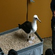
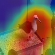
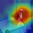
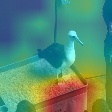
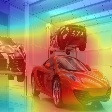
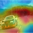
Show Cases. Authors in [8] show that the spatial attention map plays a critical role in knowledge transfer. We demonstrate the effect of representation disentanglement by visualizing the attention map in Fig 2. As observed in typical cases from CUB-200-2011 and Stanford Cars, the original representations generated by the ImageNet pre-trained model usually contain a wide range of semantic features, such as objects or backgrounds, in addition to parts of birds. Our proposed disentangler is able to “purify” the interested concepts into the positive part, while the negative part pays more attention to the complementary constituent.

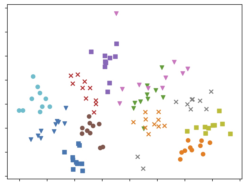
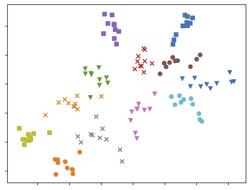
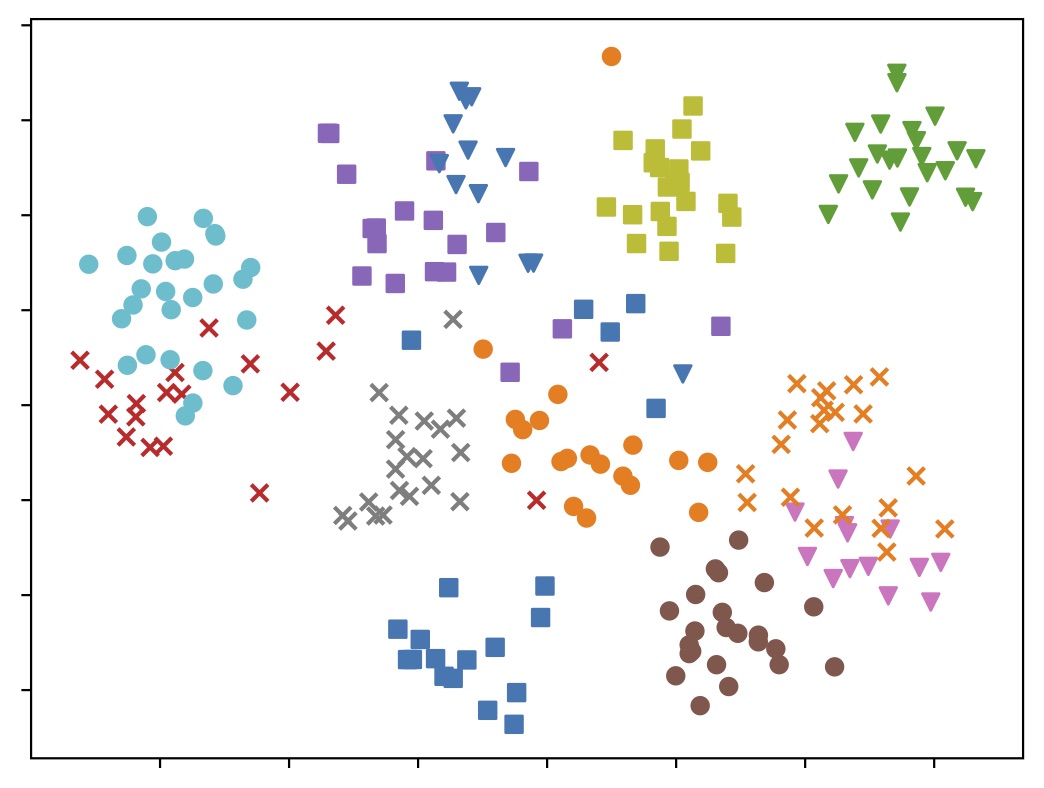
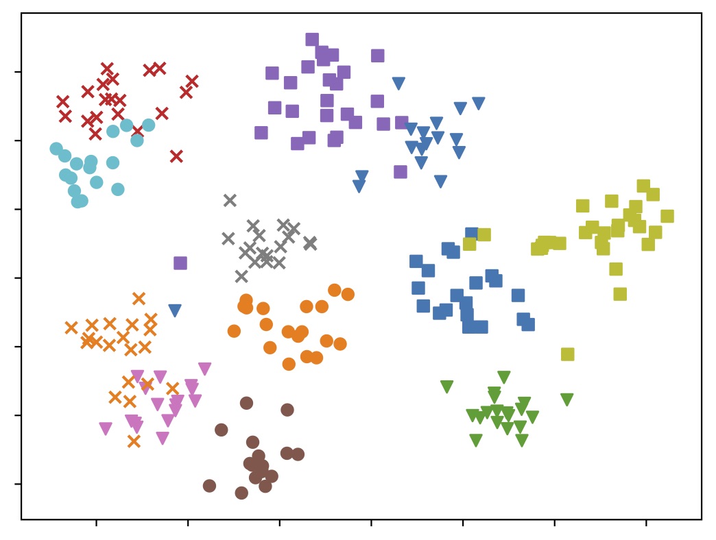
Embedding Visualization. Since the most important change of our method is to use the disentangled rather than the original representation as the reference, we are interested in comparing the properties of these two representations on the target task. We visualize the original and disentangled feature representations of Flower-102 and MIT Indoor-67. The dimension of features is reduced along the spatial direction and then plotted in the 2D space using t-SNE embeddings. As illustrated in Figure 3, deep representations derived by our proposed disentangler are separated more clearly than the original ones for different categories and clustered more tightly for samples of the same category.

VI-B Shrinking Towards True Behavior

Recent work [5] discusses the connection between their proposed $\mathrm{L^{2}\text{-}SP}$ and classical statistical theory of shrinkage estimation [15]. The key hypothesis is that shrinking towards a value which is close to the “true parameters” is more effective than an arbitrary one.  [5] argues that the starting point is supposed to be more close to the “true parameters” than zero. [8, 10] regularize the feature rather than the parameter, which can be interpreted as shrinking towards the “true behavior”. Our proposed $\mathrm{TRED}$ further improves them by explicitly disentangling “truer behavior” by utilizing the global distribution and supervision information of the target dataset. To support the claim, We provide some additional evidences as followed.

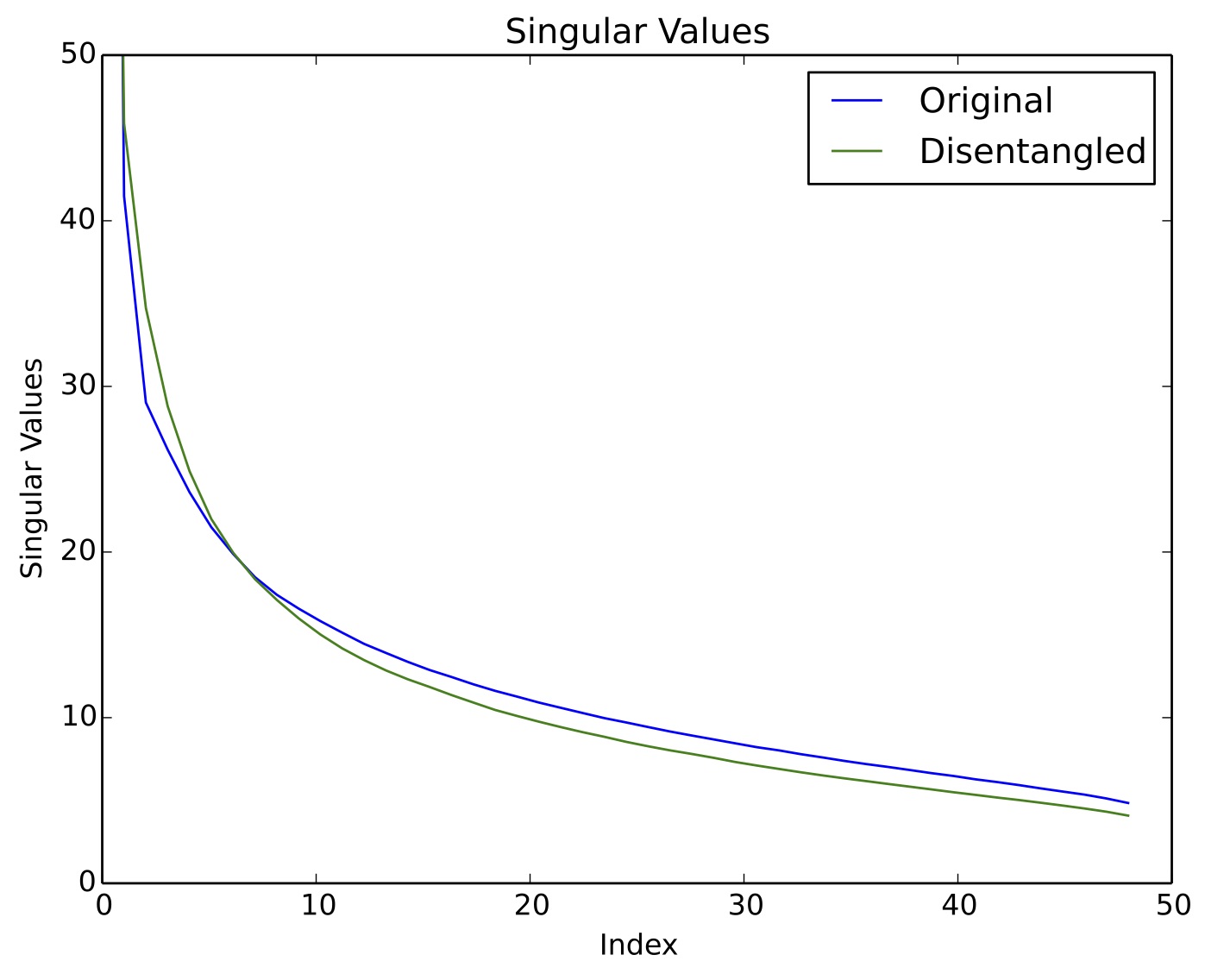
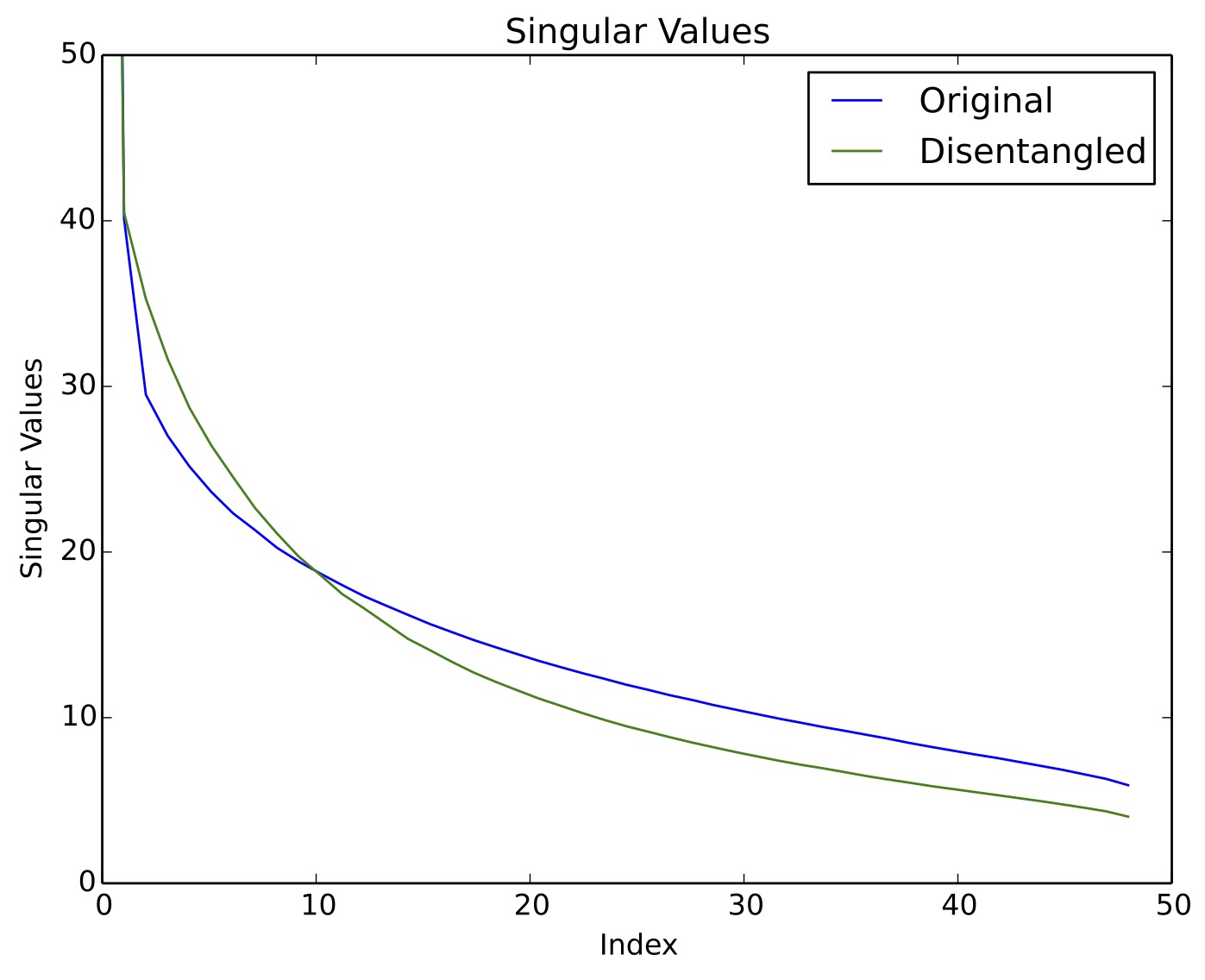
Reducing Untransferable Components. We compute singular eigenvectors and values of the deep representation by SVD. All singular values are sorted in descending order and plotted in Fig 4. Authors in [12] demonstrate that the spectral components corresponding to smaller singular values are less transferable. They find that these less transferable components can be suppressed by involving more training examples. Interestingly, we find similar trends by the proposed representation disentanglement. As observed in Fig 4, smaller singular values of the disentangled positive representation are further reduced compared with the original representation. Fig 4 also shows the phenomenon that spectral components corresponding to larger singular values are increased, which does not exist in [12]. This is intuitively consistent to the hypothesis that features relevant to the target task are disentangled and strengthened.

Robustness to Regularization Strength. We also provide an empirical evidence to illustrate the effect of “truer behavior” obtained by our proposed disentangler. The intuition is very straightforward that, if the behavior (representation) used as the reference is “truer”, it is supposed to be more robust to the larger regularization strength. We compare with $\mathrm{DELTA}$ which uses the original representation as the reference. We select three transfer learning tasks for evaluation, which are Places365 $\rightarrow$ MIT indoor-67, ImageNet $\rightarrow$ Stanford Cars and Places365 $\rightarrow$ Stanford Dogs. The regularization strength $\alpha$ is gradually increased from 0.001 to 1. As illustrated in Fig 5, the performance of $\mathrm{DELTA}$ falls rapidly as $\alpha$ increases, especially in ImageNet $\rightarrow$ Stanford Cars and Places365 $\rightarrow$ Stanford Dog, indicating that the regularizer using original representations as the reference suffers from negative transfer seriously. While $\mathrm{TRED}$ performs much more robust to the increasing of $\alpha$.

Figure 5: Top-1 accuracy of transfer learning tasks corresponding to different regularization strength $\alpha$.

Table III: Top-1 accuracy (%) of the target and source task. $\mathrm{TRED}$- refers to $\mathrm{TRED}$ without disentanglement.

Dataset	Target Task		Source Task
	$\mathrm{TRED}$	$\mathrm{TRED}$-	$\mathrm{TRED}$	$\mathrm{TRED}$-
Flower-102	91.34	89.79	71.23	69.73
CUB-200-2011	82.07	78.84	72.65	70.11
MIT Inddors 67*	85.79	82.42	28.92	25.57

• Pre-trained on Places365 and evaluated on ImageNet.

VI-C Mechanism Analysis

In this part, we briefly discuss about the necessity and relationship of the main components in our method. As our purpose is to disentangle the knowledge which is relevant to the target task, the supervision from the target dataset is of course necessary. We will first discuss whether a simple supervision is enough to “disentangle” the relevant knowledge from the source model. Next we will explain why the component of reconstruction is essential to ensure the effectiveness.

Why disentanglement is useful. It seems reasonable to obtain the discriminative representation only using the classifier corresponding to $L^{D}_{ce}$. This is equivalent to perform a pre-adaptation upon the source model before fine-tuning. Unfortunately, such straightforward adaptation in a pure supervised manner is prone to over-fitting the limited target examples, as which the resultant representation is not adequate to serve as the prior knowledge. Encouraging the disentanglement between the relevant and irrelevant part, however, provides a distribution-level guarantee to simultaneously preserve the generalization capacity of the source model and adapt for the new task. That is achieved by restricting the integrity of the underlying data structure in a self-supervised way, e.g. disentanglement and reconstruction. To verify the hypothesis, we conduct an ablation study to compare the simpler framework without the disentanglement part, which performs direct transformation on the original representation. This version is denoted by $\mathrm{TRED}$-.

We can observe in Table III that, all evaluated tasks get significant performance drop on the target task without disentanglement. A reasonable guess is that, disentangling helps preserve knowledge in the source model and restrain the representation transformation from over-fitting the classifier $C$. To verify this hypothesis, we compare the top-1 accuracy of ImageNet classification (the source task) between $\mathrm{TRED}$ (we only use $\mathrm{TRED}$-MMD here) and $\mathrm{TRED}$-. Specifically, we train a random initialized classifier to recognize the category of ImageNet, using the fixed transformed representation as input. The top-1 accuracy of the pre-trained ResNet-101 model is 75.99%. As shown in Table III, $\mathrm{TRED}$- gets more performance drops on ImageNet than $\mathrm{TRED}$, indicating that representation disentanglement performs better in preserving the general knowledge learned by the source task.

The interdependence between disentanglement and reconstruction. Disentanglement and reconstruction compose a complete self-supervised requirement. Without the force of disentanglement between the positive and negative part, the transformation will fall into the case of no disentanglement. Therefore, the reconstruction requirement alone is not capable of ensuring the preservation of the source knowledge of the learned positive part. Removing the reconstruction requirement results in an analogy situation, as the transformation can be arbitrary, pursuing to enlarge the discrepancy or independence between the two parts with no knowledge constraint. Intuitively, given that the positive part focus on the supervision information, the negative part can be easily learned to adapt either one (alone) of the two requirements. That causes both cases are almost equivalent to removing the entire disentangler.

In condition of the reconstruction guarantee, maximizing the attention discrepancy or minimizing the semantic independence between the positive and negative part encourages the two parts to focus on patterns related with different semantic concepts, with as less overlaps or interactions as possible. This is exact a form of representation disentanglement. For example the positive part is activated on heads and feathers of birds, while the negative part is activated on objects such as trees and wires as shown in Fig. 2. Moreover, this is achieved at a distribution level so that the semantic separation is consistent in the entire dataset.

VII Conclusion

In this paper, we extend the study of catastrophic forgetting and negative transfer in inductive transfer learning. Specifically, we propose a novel approach $\mathrm{TRED}$ to regularize the disentangled deep representation, achieving accurate knowledge transfer. We succeed to implement the target-awareness disentanglement, by maximizing the Maximum Mean Discrepancy (MMD) on visual attentions and minimizing the Mutual Information (MI) on semantic features. Extensive experimental results on various real-world transfer learning datasets show that $\mathrm{TRED}$ significantly outperforms the state-of-the-art transfer learning regularizers. Moreover, we provide empirical analysis to verify that the disentangled target-awareness representation is closer to the expected “true behavior” of the target task.

Michael Shell Biography text here.

John Doe Biography text here.

Jane Doe Biography text here.

References

- [1] O. Russakovsky, J. Deng, H. Su, J. Krause, S. Satheesh, S. Ma, Z. Huang, A. Karpathy, A. Khosla, M. Bernstein et al., “Imagenet large scale visual recognition challenge,” International journal of computer vision, vol. 115, no. 3, pp. 211–252, 2015.
- [2] B. Zhou, A. Lapedriza, A. Khosla, A. Oliva, and A. Torralba, “Places: A 10 million image database for scene recognition,” IEEE transactions on pattern analysis and machine intelligence, vol. 40, no. 6, pp. 1452–1464, 2017.
- [3] J. Yosinski, J. Clune, Y. Bengio, and H. Lipson, “How transferable are features in deep neural networks?” in Advances in neural information processing systems, 2014, pp. 3320–3328.
- [4] S. J. Pan and Q. Yang, “A survey on transfer learning,” IEEE Transactions on knowledge and data engineering, vol. 22, no. 10, pp. 1345–1359, 2009.
- [5] X. Li, Y. Grandvalet, and F. Davoine, “Explicit inductive bias for transfer learning with convolutional networks,” Thirty-fifth International Conference on Machine Learning, 2018.
- [6] J. Kirkpatrick, R. Pascanu, N. Rabinowitz, J. Veness, G. Desjardins, A. A. Rusu, K. Milan, J. Quan, T. Ramalho, A. Grabska-Barwinska et al., “Overcoming catastrophic forgetting in neural networks,” Proceedings of the national academy of sciences, vol. 114, no. 13, pp. 3521–3526, 2017.
- [7] G. Hinton, O. Vinyals, and J. Dean, “Distilling the knowledge in a neural network,” arXiv preprint arXiv:1503.02531, 2015.
- [8] S. Zagoruyko and N. Komodakis, “Paying more attention to attention: Improving the performance of convolutional neural networks via attention transfer,” arXiv preprint arXiv:1612.03928, 2016.
- [9] J. Yim, D. Joo, J. Bae, and J. Kim, “A gift from knowledge distillation: Fast optimization, network minimization and transfer learning,” in The IEEE Conference on Computer Vision and Pattern Recognition (CVPR), vol. 2, 2017.
- [10] X. Li, H. Xiong, H. Wang, Y. Rao, L. Liu, and J. Huan, “Delta: Deep learning transfer using feature map with attention for convolutional networks,” arXiv preprint arXiv:1901.09229, 2019.
- [11] L. Torrey and J. Shavlik, “Transfer learning,” in Handbook of research on machine learning applications and trends: algorithms, methods, and techniques. IGI global, 2010, pp. 242–264.
- [12] X. Chen, S. Wang, B. Fu, M. Long, and J. Wang, “Catastrophic forgetting meets negative transfer: Batch spectral shrinkage for safe transfer learning,” in Advances in Neural Information Processing Systems, 2019, pp. 1906–1916.
- [13] J. Donahue, Y. Jia, O. Vinyals, J. Hoffman, N. Zhang, E. Tzeng, and T. Darrell, “Decaf: A deep convolutional activation feature for generic visual recognition,” in International conference on machine learning, 2014, pp. 647–655.
- [14] C. Stein, “Inadmissibility of the usual estimator for the mean of a multivariate normal distribution,” Stanford University Stanford United States, Tech. Rep., 1956.
- [15] B. Efron and C. Morris, “Stein’s paradox in statistics,” Scientific American, vol. 236, no. 5, pp. 119–127, 1977.
- [16] C. Chelba and A. Acero, “Adaptation of maximum entropy capitalizer: Little data can help a lot,” Computer Speech & Language, vol. 20, no. 4, pp. 382–399, 2006.
- [17] J. Yang, R. Yan, and A. G. Hauptmann, “Adapting svm classifiers to data with shifted distributions,” in Seventh IEEE International Conference on Data Mining Workshops (ICDMW 2007). IEEE, 2007, pp. 69–76.
- [18] X. Li, Regularized adaptation: Theory, algorithms and applications. Citeseer, 2007, vol. 68.
- [19] Y. Aytar and A. Zisserman, “Tabula rasa: Model transfer for object category detection,” in 2011 international conference on computer vision. IEEE, 2011, pp. 2252–2259.
- [20] Y. Bengio, “Deep learning of representations for unsupervised and transfer learning,” in Proceedings of ICML workshop on unsupervised and transfer learning, 2012, pp. 17–36.
- [21] M. Oquab, L. Bottou, I. Laptev, and J. Sivic, “Learning and transferring mid-level image representations using convolutional neural networks,” in Proceedings of the IEEE conference on computer vision and pattern recognition, 2014, pp. 1717–1724.
- [22] H. Liu, M. Long, J. Wang, and M. I. Jordan, “Towards understanding the transferability of deep representations,” arXiv preprint arXiv:1909.12031, 2019.
- [23] W. Ge and Y. Yu, “Borrowing treasures from the wealthy: Deep transfer learning through selective joint fine-tuning,” in Proceedings of the IEEE conference on computer vision and pattern recognition, 2017, pp. 1086–1095.
- [24] J. Ngiam, D. Peng, V. Vasudevan, S. Kornblith, Q. V. Le, and R. Pang, “Domain adaptive transfer learning with specialist models,” arXiv preprint arXiv:1811.07056, 2018.
- [25] Y. Jeon, Y. Choi, J. Park, S. Yi, D. Cho, and J. Kim, “Sample-based regularization: A transfer learning strategy toward better generalization,” arXiv preprint arXiv:2007.05181, 2020.
- [26] Y. Guo, H. Shi, A. Kumar, K. Grauman, T. Rosing, and R. Feris, “Spottune: transfer learning through adaptive fine-tuning,” in Proceedings of the IEEE Conference on Computer Vision and Pattern Recognition, 2019, pp. 4805–4814.
- [27] K. Wang, X. Gao, Y. Zhao, X. Li, D. Dou, and C.-Z. Xu, “Pay attention to features, transfer learn faster cnns,” in International Conference on Learning Representations, 2019.
- [28] D. Hu, X. Li, L. Mou, P. Jin, D. Chen, L. Jing, X. Zhu, and D. Dou, “Cross-task transfer for multimodal aerial scene recognition,” arXiv preprint arXiv:2005.08449, 2020.
- [29] I. Goodfellow, H. Lee, Q. V. Le, A. Saxe, and A. Y. Ng, “Measuring invariances in deep networks,” in Advances in neural information processing systems, 2009, pp. 646–654.
- [30] Y. Bengio, A. Courville, and P. Vincent, “Representation learning: A review and new perspectives,” IEEE transactions on pattern analysis and machine intelligence, vol. 35, no. 8, pp. 1798–1828, 2013.
- [31] I. Goodfellow, J. Pouget-Abadie, M. Mirza, B. Xu, D. Warde-Farley, S. Ozair, A. Courville, and Y. Bengio, “Generative adversarial nets,” in Advances in neural information processing systems, 2014, pp. 2672–2680.
- [32] D. P. Kingma and M. Welling, “Auto-encoding variational bayes,” arXiv preprint arXiv:1312.6114, 2013.
- [33] X. Chen, Y. Duan, R. Houthooft, J. Schulman, I. Sutskever, and P. Abbeel, “Infogan: Interpretable representation learning by information maximizing generative adversarial nets,” in Advances in neural information processing systems, 2016, pp. 2172–2180.
- [34] A. Odena, C. Olah, and J. Shlens, “Conditional image synthesis with auxiliary classifier gans,” in Proceedings of the 34th International Conference on Machine Learning-Volume 70. JMLR. org, 2017, pp. 2642–2651.
- [35] I. Higgins, L. Matthey, A. Pal, C. Burgess, X. Glorot, M. Botvinick, S. Mohamed, and A. Lerchner, “beta-vae: Learning basic visual concepts with a constrained variational framework.” ICLR, vol. 2, no. 5, p. 6, 2017.
- [36] H. Kim and A. Mnih, “Disentangling by factorising,” arXiv preprint arXiv:1802.05983, 2018.
- [37] Y.-C. Liu, Y.-Y. Yeh, T.-C. Fu, S.-D. Wang, W.-C. Chiu, and Y.-C. Frank Wang, “Detach and adapt: Learning cross-domain disentangled deep representation,” in Proceedings of the IEEE Conference on Computer Vision and Pattern Recognition, 2018, pp. 8867–8876.
- [38] A. H. Liu, Y.-C. Liu, Y.-Y. Yeh, and Y.-C. F. Wang, “A unified feature disentangler for multi-domain image translation and manipulation,” in Advances in Neural Information Processing Systems, 2018, pp. 2590–2599.
- [39] X. Peng, Z. Huang, X. Sun, and K. Saenko, “Domain agnostic learning with disentangled representations,” arXiv preprint arXiv:1904.12347, 2019.
- [40] M. I. Belghazi, A. Baratin, S. Rajeswar, S. Ozair, Y. Bengio, A. Courville, and R. D. Hjelm, “Mine: mutual information neural estimation,” arXiv preprint arXiv:1801.04062, 2018.
- [41] M. Soltanolkotabi, A. Javanmard, and J. D. Lee, “Theoretical insights into the optimization landscape of over-parameterized shallow neural networks,” IEEE Transactions on Information Theory, vol. 65, no. 2, pp. 742–769, 2018.
- [42] A. Romero, N. Ballas, S. E. Kahou, A. Chassang, C. Gatta, and Y. Bengio, “Fitnets: Hints for thin deep nets,” CoRR, vol. abs/1412.6550, 2014.
- [43] A. Gretton, K. M. Borgwardt, M. J. Rasch, B. Schölkopf, and A. Smola, “A kernel two-sample test,” The Journal of Machine Learning Research, vol. 13, no. 1, pp. 723–773, 2012.
- [44] S. J. Pan, I. W. Tsang, J. T. Kwok, and Q. Yang, “Domain adaptation via transfer component analysis,” IEEE Transactions on Neural Networks, vol. 22, no. 2, pp. 199–210, 2010.
- [45] E. Tzeng, J. Hoffman, N. Zhang, K. Saenko, and T. Darrell, “Deep domain confusion: Maximizing for domain invariance,” arXiv preprint arXiv:1412.3474, 2014.
- [46] M. Long, H. Zhu, J. Wang, and M. I. Jordan, “Deep transfer learning with joint adaptation networks,” in Proceedings of the 34th International Conference on Machine Learning-Volume 70. JMLR. org, 2017, pp. 2208–2217.
- [47] D. J. Sutherland, H.-Y. Tung, H. Strathmann, S. De, A. Ramdas, A. Smola, and A. Gretton, “Generative models and model criticism via optimized maximum mean discrepancy,” arXiv preprint arXiv:1611.04488, 2016.
- [48] M. Arbel, D. Sutherland, M. Bińkowski, and A. Gretton, “On gradient regularizers for mmd gans,” in Advances in Neural Information Processing Systems, 2018, pp. 6700–6710.
- [49] M. Long, Y. Cao, J. Wang, and M. Jordan, “Learning transferable features with deep adaptation networks,” in International conference on machine learning. PMLR, 2015, pp. 97–105.
- [50] C. Louizos, K. Swersky, Y. Li, M. Welling, and R. S. Zemel, “The variational fair autoencoder,” in ICLR, 2016.
- [51] A. Khosla, N. Jayadevaprakash, B. Yao, and L. Fei-Fei, “Novel dataset for fine-grained image categorization,” in First Workshop on Fine-Grained Visual Categorization, IEEE Conference on Computer Vision and Pattern Recognition, Colorado Springs, CO, June 2011.
- [52] A. Quattoni and A. Torralba, “Recognizing indoor scenes,” in 2009 IEEE Conference on Computer Vision and Pattern Recognition. IEEE, 2009, pp. 413–420.
- [53] P. Welinder, S. Branson, T. Mita, C. Wah, F. Schroff, S. Belongie, and P. Perona, “Caltech-UCSD Birds 200,” California Institute of Technology, Tech. Rep. CNS-TR-2010-001, 2010.
- [54] M.-E. Nilsback and A. Zisserman, “Automated flower classification over a large number of classes,” in 2008 Sixth Indian Conference on Computer Vision, Graphics & Image Processing. IEEE, 2008, pp. 722–729.
- [55] J. Krause, M. Stark, J. Deng, and L. Fei-Fei, “3d object representations for fine-grained categorization,” in 4th International IEEE Workshop on 3D Representation and Recognition (3dRR-13), Sydney, Australia, 2013.
- [56] O. M. Parkhi, A. Vedaldi, A. Zisserman, and C. Jawahar, “Cats and dogs,” in 2012 IEEE conference on computer vision and pattern recognition. IEEE, 2012, pp. 3498–3505.
- [57] M. Cimpoi, S. Maji, I. Kokkinos, S. Mohamed, , and A. Vedaldi, “Describing textures in the wild,” in Proceedings of the IEEE Conf. on Computer Vision and Pattern Recognition (CVPR), 2014.
- [58] K. He, X. Zhang, S. Ren, and J. Sun, “Deep residual learning for image recognition,” in Proceedings of the IEEE conference on computer vision and pattern recognition, 2016, pp. 770–778.
- [59] T. Van Laarhoven, “L2 regularization versus batch and weight normalization,” arXiv preprint arXiv:1706.05350, 2017.
- [60] A. S. Golatkar, A. Achille, and S. Soatto, “Time matters in regularizing deep networks: Weight decay and data augmentation affect early learning dynamics, matter little near convergence,” in Advances in Neural Information Processing Systems, 2019, pp. 10 678–10 688.