The assembly bias of emission line galaxies

Abstract

The next generation of spectroscopic surveys will target emission-line galaxies (ELGs) to produce constraints on cosmological parameters. We study the large scale structure traced by ELGs using a combination of a semi-analytical model of galaxy formation, a code that computes the nebular emission from HII regions using the properties of the interstellar medium, and a large-volume, high-resolution N-body simulation. We consider fixed number density samples where galaxies are selected by either their H$\alpha$, [OIII]$\lambda 5007$ or [OII]$\lambda\lambda 3727-3729$ emission line luminosities. We investigate the assembly bias signatures of these samples, and compare them to those of stellar mass and SFR selected samples. Interestingly, we find that the [OIII]- and [OII]-selected samples display scale-dependent bias on large scales and that their assembly bias signatures are also scale-dependent. Both these effects are more pronounced for lower number density samples. The [OIII] and [OII] emitters that contribute most to the scale dependence tend to have a low gas-phase metallicity and are preferentially found in low-density regions. We also measure the baryon acoustic oscillation (BAO) feature and the $\beta$ parameter related to the growth rate of overdensities. We find a slight tendency for the BAO peak to shift toward smaller scales for [OII] emitters and that $\beta$ is scale-dependent at large scales. Our results suggest that ELG samples include environmental effects that should be modelled in order to remove potential systematic errors that could affect the estimation of cosmological parameters.

1 Introduction

Mapping the Universe using photometric and spectroscopic surveys allows us to measure the cosmic large-scale structure which encodes valuable cosmological information. However, since the galaxy distribution is not a direct tracer of the underlying density field it is essential to understand the connection between galaxies and dark matter haloes to obtain an accurate interpretation of the Universe (for a review see Wechsler & Tinker 2018). A relevant statistical property of the galaxy distribution is the clustering signal which is often quantified using the two-point correlation function (2PCF). Measuring galaxy clustering allows us to extract two pieces of information that can be used to constrain the cosmological model (Weinberg et al., 2013): (i) the scale of standard ruler features, such as the baryonic acoustic oscillation (BAO) peak, from which we can obtain the cosmic expansion history, and (ii) the magnitude of redshift-space distortions (RSD) in the clustering signal, which are driven by the rate at which structure grows. Both of these quantities depend on the amount of dark matter and dark energy.

Precise measurements of BAO and RSD are difficult to obtain because cosmic (sample) variance and shot noise are significant when the sampled volume is small (Kaiser, 1986a). The Sloan Digital Sky Survey (SDSS) and the 2dF Galaxy Redshift Survey (2dFGRS) were the first to observe hundreds of thousands of galaxies in large volumes, obtaining convincing detections of the BAO (Eisenstein et al., 2005; Cole et al., 2005). Observations have continued throughout the last fifteen years mostly using massive luminous red galaxies (LRGs) as the tracers of the large-scale structure (e.g Eisenstein et al., 2011; Zehavi et al., 2011; Dawson et al., 2013; Bautista et al., 2018).

Advances in wide field spectroscopy have opened up the opportunity to trace the large-scale structure using emission-line galaxies (ELGs). The nebular emission of these galaxies is produced by gas in HII regions which is photoionized by radiation from young stars. Some emission line luminosities have therefore been used to infer star formation rates, although in general the relation between line emission and SFR can be complicated as the emission depends on the local properties of the ISM such as gas metallicity, temperature and density (e.g Levesque et al., 2010; Gutkin et al., 2016; Byler et al., 2017) and on the attenuation by dust of the line luminosity. Moreover, ELGs do not trace the field in the same way as LRGs; ELGs tend to reside in low mass haloes (Favole et al., 2016; Gonzalez-Perez et al., 2018) and live in filaments and sheets rather than in the knots of the cosmic web occupied by LRGs (Gonzalez-Perez et al., 2020).

Typically, given the depth of upcoming surveys with spectrographs that operate in the optical, ELG catalogues have redshift distributions that peak around $z\sim 1$ which, in combination with Ly$\alpha$ emitters at $z\gtrsim 2$, enables us to investigate the history of cosmic expansion at previously unexplored epochs. The SDSS-IV/eBOSS survey (Dawson et al., 2016) provides one of the largest ELG catalogues to date, and the next generation of surveys like DESI (DESI Collaboration et al., 2016) and Euclid (Laureijs et al., 2011) will detect millions of ELGs. This will potentially enable us to measure cosmological parameters with exceptional precision.

To fully exploit the future ELG data it is essential to understand any systematic effects that may influence the inferred cosmological constraints. Galaxy formation models can be used for this purpose, to provide insights into the galaxy-halo connection with the by-product of testing different prescriptions for the physical processes that regulate galaxy evolution. A useful approach to explore galaxy formation is to use semi-analytical models (SAMs Cole et al., 2000; Baugh, 2006; Somerville et al., 2008). These models use simplified descriptions of physical processes that shape the fate of baryons within the dark matter halo merger trees extracted from N-body dark matter only simulations, expressed in a set of coupled differential equations with parameters to encapsulate “sub-grid” physics. SAMs can successfully reproduce, amongst other things, the observed luminosity and stellar mass functions (e.g Croton et al., 2006; Henriques et al., 2015; Croton et al., 2016; Stevens et al., 2016; Lagos et al., 2018; Baugh et al., 2019). Alternatively, hydrodynamical simulations offer a complementary approach to follow baryonic physics, which in general requires fewer assumptions and approximations than are needed in SAMs, but which nevertheless still appeal to using sub-grid recipes for unresolved processes (e.g Vogelsberger et al., 2014; Schaye et al., 2015; Nelson et al., 2018). Due to the higher computational overhead of hydrodynamical simulations compared with SAMs, the largest volumes probed by state-of-the-art hydrodynamical simulations are still 10-100 times smaller than the typical SAM volume.

Another approach used to connect galaxies with their host haloes is to employ an empirical model such as the halo occupation distribution (HOD) framework (e.g Benson et al., 2000; Scoccimarro et al., 2001; Berlind & Weinberg, 2002; Kravtsov et al., 2004; Zheng et al., 2005). The HOD provides an empirical relation between the average number of galaxies $\rm N$ hosted by haloes with mass $\rm M$. This relation is characterized by a probability distribution $\rm P(N|M)$ that depends on the redshift, number density and selection criteria of a galaxy sample. Here, the standard assumption is that the galaxy content depends only on halo mass, but this may not be true if the galaxy distribution correlates with the assembly history of haloes. N-body simulations have shown that the clustering of dark matter haloes does depend on secondary halo properties like formation time, concentration and spin (e.g Gao et al., 2005; Gao & White, 2007; Wechsler et al., 2006), an effect called halo assembly bias. Likewise, the manifestation of assembly bias in galaxy clustering, commonly referred to as galaxy assembly bias, has been found both in SAMs (e.g Croton et al., 2007; Contreras et al., 2019; Zehavi et al., 2018, 2019; Jiménez et al., 2019; Xu et al., 2020) and hydrodynamical simulations (e.g Artale et al., 2018; Xu & Zheng, 2020; Montero-Dorta et al., 2020). Assessing the existence of assembly bias in the real Universe is an important task; cosmological constraints from future surveys will most likely be limited by how well we can model the observations rather than the precision of the measurements.

In general, assembly bias enhances the clustering amplitude on large scales for stellar mass selected samples and suppresses it for SFR selections (Contreras et al., 2019, 2020). However, as we found in these studies, these trends can change depending on the number density and redshift of the sample. So far, there are no direct measurements of the assembly bias signature in ELG catalogues, but, in principle, the effect should be similar to that reported for SFR selections as ELGs are a subset of star-forming galaxies.

Here we aim to study the large-scale structure of ELGs by measuring the clustering and galaxy assembly bias signature of these samples. We employ galaxies from the SAG semi-analytical model (Cora et al., 2018) run on the MultiDark Planck cosmological simulation (Klypin et al., 2016). The total simulated volume is ${\rm(1}\ h^{-1}{\rm Gpc)^{3}}$, so the effect of the sample variance is greatly reduced. Thus, we can accurately sample the 2PCF up to scales of the BAO feature and determine whether or not the impact of assembly bias from ELG selections is significant. We calculate the nebular emission in SAG galaxies using the GET_EMLINES code from Orsi et al. (2014), and then store the H$\alpha$, [OIII] and [OII] line emission luminosities. These emission lines at $\rm z\sim 1$ correspond either to the near-infrared and optical range sampled by DESI and Euclid, respectively.

The layout of the paper is as follows. Section 2 describes the SAG galaxy formation model and the N-body simulation in which it is implemented, along with how we define our galaxy samples, while in Section 3 we compare and characterize these samples. In Section 4 we show the assembly bias signatures, and in Section 5 we study a possible origin for features in the assembly bias of ELGs. The BAO and the $\beta$ parameter, which quantifies the strength of anisotropies produced by the RSD, are shown in Section 6 for each sample. We conclude in Section 7. Brief discussions about results from other SAMs, and ELG sample completeness, are presented in Appendix A and B, respectively.

Throughout the paper masses are measured in $h^{-1}\rm M_{\odot}$, the SFR is measured in $h^{-1}\rm M_{\odot}yr^{-1}$ and distances are measured in $h^{-1}\rm Mpc$ and are in comoving units.

2 Simulation data

2.1 The galaxy formation model: SAG

Here we use the Semi-Analytical Galaxies (SAG) model of galaxy formation (Cora, 2006). Semi-analytical models use the merger trees extracted from N-Body simulations to model the main physical processes involved in the evolution of a galaxy, such as the treatment of radiative cooling of hot gas, star formation, feedback effects from supernovae and active galactic nucleus (AGN) feedback, chemical enrichment of the gas, the growth of supermassive black holes, and the impact from galaxy mergers, among others.

The version of SAG used in this work is the one presented in Cora et al. (2018), which uses the outputs of the MultiDark2 cosmological simulation (hereafter MDPL2, Klypin et al. 2016, see section 2.2 for more details). The main output of the simulation and the SAM are publicly available as a part of the MultiDark comparison project (Knebe et al., 2018). The SAG SAM was originally presented in Cora (2006) and is based on the model by Springel et al. (2001). Since then the code has been through several updates (Lagos et al., 2008; Tecce et al., 2010; Orsi et al., 2014; Padilla et al., 2014; Muñoz Arancibia et al., 2015; Gargiulo et al., 2015) and is capable of reproducing observations both at low and high redshift. One of the key features of this model is the use of particle swarm optimization technique (PSO) to automatically set the model parameters by requiring the output to fit several observables (Ruiz et al., 2015).

The galaxy properties produced by this model include stellar mass, cold gas, black hole and bulge masses, the average and instantaneous star formation rates (SFR), where the latter corresponds to the SFR in the most recent time sub-step, which is a subdivision of the timestep between the simulation snapshots. Sub-step sizes range from 5 and 15 Myr, whereas the time between snapshots is of the order of 100 Myr. These quantities are computed separately for disks and bulges, where the former are the result of quiescent star formation in cooled gas disks and the latter form via starburst episodes. The gas-phase metallicity for both components is calculated by modelling the chemical enrichment of the ISM, which takes into account mass loss from massive stars and supernovae. These two ways to compute the SFR are important when computing the emission line fluxes of the galaxies (see section 2.3 for more details).

2.2 The MultiDark Planck 2 simulation

As mentioned in the previous section, SAG was run on the halo merger trees from the MULTIDARK simulation MDPL2 (Klypin et al., 2016). The MDPL2 adopts a $\Lambda$CDM Universe, charaterized by Planck cosmological parameters (Planck Collaboration et al., 2014): $\Omega_{\rm m}=0.307$, $\Omega_{\rm b}=0.048$, $\Omega_{\Lambda}=0.693$, $h=0.678$ and $n_{\rm s}=0.96$. The simulation follows $3840^{3}$ particles within a cubic box of comoving side-length $1\ h^{-1}\rm Gpc$, with a mass resolution of ${\rm m_{p}=1.51\times 10^{9}}h^{-1}{\rm M_{\odot}}$. The particles are followed from $z=120$ until z=0 and their positions and velocities are output at 126 snaphots. The dark matter haloes are identified with the ROCKSTAR halo finder (Behroozi et al., 2013a), and the CONSISTENT TREES code (Behroozi et al., 2013b) is used to construct the merger trees. These halo finder and halo merger tree algorithms identify objects in phase space, keeping a better track of the substructures after their infall.

The large cosmological volume of the MDPL2 allows us to make accurate clustering measurements up to scale separations that encapsulate useful cosmological information.

2.3 The calculation of nebular emission

To model the nebular emission of the star-forming galaxies we use the GET_EMLINES model introduced by Orsi et al. (2014) (hereafter O14) to post-process the output from the SAG model. The GET_EMLINES code uses the output of the photoionisation code MAPPINGS-III (Dopita & Sutherland, 1995; Groves et al., 2004), as tabulated by Levesque et al. (2010). MAPPINGS-III predicts the nebular emission from HII regions. The grid calculated by Levesque et al. (2010) tabulates the emission line fluxes as a function of the gas-phase metallicity and the ionization parameter of the HII region, $q$. O14 uses the gas metallicities of the bulges and disks from the SAG galaxies, but it does not predict the ionization parameter within individual HII regions due to a lack of resolution to resolve the internal structure of galaxies. Instead, O14 advocated a model in which $q$ could be inferred from the gas-phase metallicity, an assumption which is inspired by observational results which suggest that $q$ is anti-correlated with the metallicity of the cold star-forming gas (e.g Nagao et al., 2006; Groves & Allen, 2010; Shim & Chary, 2013). O14 show that parameters selected in their model to calculate $q$ from the gas phase metallicity allowed the SAG model to reproduce the locus of star forming galaxies in the so-called BPT diagram relating the line ratios [OIII$\lambda$5007]/H$\beta$ and [NII$\lambda$6854]/H$\alpha$ (Baldwin et al., 1981).cNote that O14 showed that the predictions were robust to substantial perturbations to the parameter values in the model for $q$. Ideally, the GET_EMLINES code uses the instantaneous SFR rather than a time-averaged SFR, as the instantaneous SFR is a better indicator of the number of Lyman continuum photons which make up the ionising radiation field and, as a consequence, of the H$\alpha$ luminosity. Nevertheless, Favole et al. (2020) used the averaged SFR predicted by the SAGE (Croton et al., 2016) and GALACTICUS (Benson, 2012) SAMs to infer the [OII] line emission, and found reasonable agreement with observational data at $z\sim 1$.

We use GET_EMLINES and instantaneous SFRs to compute the luminosities for the H$\alpha$, [OIII]$\lambda 5007$, [OII]$\lambda\lambda 3727-3729$ and [NII]$\lambda\lambda 6548-6584$ emission lines (hereafter H$\alpha$, [OIII], [OII] and [NII] respectively). As these values are calculated separately for the bulge and disk components of a galaxy, we sum these contributions to obtain the total nebular emission for each galaxy. Note that we do not apply any attenuation to the line luminosity.

2.4 The galaxy samples

We use galaxy samples characterised by fixed number densities of objects. We achieve this by ranking the galaxies from the highest to lowest values of a given property (e.g. their emission line luminosity, averaged SFR or stellar mass), and then retaing only those galaxies above a threshold value that corresponds to the desired number density. The number densities used in this work are $n=0.001\ h^{3}{\rm Mpc^{-3}}$, $n=0.00316\ h^{3}{\rm Mpc^{-3}}$ and $n=0.01\ h^{3}{\rm Mpc^{-3}}$.

As the samples selected by line emission are star-forming galaxies, it is expected that they will have some overlap with galaxies selected by their SFR. Hence, we also include SFR selected samples and perform the same analysis on these as carried out for the ELG samples. We also consider stellar-mass selected samples to allow further comparisons with assembly bias signatures which have been studied in several galaxy formation models (e.g Artale et al., 2018; Zehavi et al., 2018; Contreras et al., 2019). The cumulative distribution functions for the different selections are shown in Fig. 1. The number densities adopted to define our samples are shown by the horizontal thin dashed lines. Note that the galaxies included in each sample are those to the right of the intersection between the cumulative functions with the horizontal lines. We also include a selection based on the combined luminosity of the H$\alpha$+doublet [NII]$\lambda\lambda 6548-6584$ lines; this combination mimics the flux that the Euclid mission will capture for its sources due to its limited spectral resolution. This allows us to assess the contribution of the [NII] flux to the predictions for H$\alpha$ (see also Merson et al. 2018).

The data used here correspond to a subsample of SAG where galaxies were selected with a stellar-mass cut of ${\rm 5\times 10^{8}}\ h^{-1}{\rm M_{\odot}}$. This cut affects the completeness of SFR and ELG selections. In Appendix B we explain that this has a negligible impact on the trends and results we obtain.

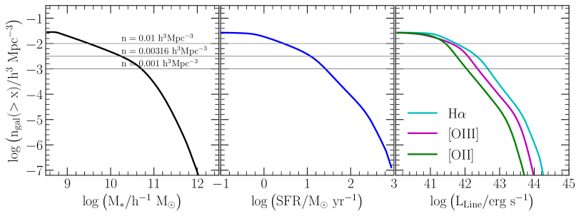
Figure 1: The cumulative distribution functions of SAG galaxies selected by stellar mass (left), SFR (middle) and $\rm H\alpha$, [OIII], [OII] line luminosities (right). The horizontal dashed lines indicate the number densities used to define our galaxy samples. Note the plateau at low SFR and $\rm L_{Line}$, which is due to a stellar mass cut in the parent catalogue, which is discussed further in Appendix B.

3 Properties of ELG selected samples

To assess the level of similarity between the ELG and star-forming galaxy samples we compare their two-point correlation functions (2PCF). The 2PCF measures the excess probability of finding a pair of objects at a separation $r$ compared to a homogeneously distributed sample. We measure the 2PCF using the CorrFunc public code presented in Sinha & Garrison (2017). The resulting 2PCF are shown in the main panel of Fig. 2 for the SFR and ELG samples with number density $n=0.00316\ h^{3}{\rm Mpc^{-3}}$; the sub-panel shows the ratios between these measurements and the 2PCF of the SFR selected sample. The first impression is that the shapes of the 2PCFs are largely similar, irrespective of separation, with variations within $10\%$. On large scales, the differences are mostly due to the different bias parameters of the samples, with the [OIII] and [OII] selected samples showing weaker clustering than the H$\alpha$ and SFR samples. On small scales, the differences may be due to the additional dependence on the physical conditions in the ISM; the H$\alpha$ emission mostly traces the SFR, but the [OIII] and [OII] emission also depends on the cold gas metallicity. Hence, differences in the one-halo terms suggest a possible connection between the spatial distribution of ELGs and the properties of their ISM. As can be seen from Fig. 2, the difference in the 2PCF compared with that measured for the SFR selected sample depends on which line is chosen to construct the sample. Both the H$\alpha$ and H$\alpha$ + [NII] selections result in an amplitude for the 2PCF that is similar to that found for the SFR selection. This is expected as the strength of H$\alpha$ emission is almost an instantaneous measure of the star formation rate, with little dependence on the metallicity of the star forming gas. The 2PCFs measured for the [OIII] and [OII] selections show a bigger difference from that found for the star formation sample, with an amplitude reduction of $\sim 20$ and $30$ per cent, respectively. This change in the effective bias parameter of these samples is related to the selection of galaxies with specific combinations of SFR and gas metallicity, as we demonstrate below.

Figure 2: The 2PCFs for SAG samples selected according to different properties, as indicated by the key; in each case the number density is $n=0.00316\ h^{3}{\rm Mpc^{-3}}$. The bottom panel shows the ratio of the correlation functions measured for each sample with respect to the SFR-selected sample.

One way to interpret the 2PCF is by using the halo occupation distribution (HOD) framework. The HOD characterises a galaxy population via the halo occupation function, the average number of galaxies as a function of the host halo mass. Whereas HODs are typically used as an empirical model with parameters which are set to reproduce the measured abundance and 2PCF of a galaxy samples, SAMs predict the form of the HOD. So, in the case of SAMs, the HOD formalism produces a concise description of the model output that can be readily interpreted in relation to the 2PCF. In general, this function is separated into the contribution from central galaxies and from satellites with specific forms that depend on the selection criteria (Zheng et al., 2005). For example, when samples are defined by luminosity or stellar mass cuts, the HOD for central galaxies follows a step-like form. When samples are defined by SFR or colour cuts, on the other hand, the HOD of centrals reaches a peak followed by a dip to values below unity as the halo mass increases (e.g Zehavi et al., 2011; Contreras et al., 2013; Gonzalez-Perez et al., 2018; Jiménez et al., 2019). The output of a SAM for these selections can be tabulated as an HOD, without having to adopt a particular parametric form, which is very powerful when considering selections for which there is little available data, such as ELGs.

Fig. 3 shows the HODs predicted by the SAG model for SFR and ELG selections with a number density $n=0.00316\ h^{3}{\rm Mpc^{-3}}$. We also show results for a stellar mass selected sample to illustrate the differences compared to the star-forming and ELG samples. The stellar mass selected sample in the figure shows the canonical step-like form for the HODs of centrals, with the HOD for satellites exhibiting a power-law behaviour. In contrast, the ELG selections show a peak in the HOD of central galaxies, which shifts to lower masses for the [OIII] and [OII] selections. This indicates that model ELGs are mostly hosted by low halo masses, consistent with previous results from simulations (e.g Gonzalez-Perez et al., 2018). For large halo masses, the HODs of both centrals and satellites increase with halo mass.

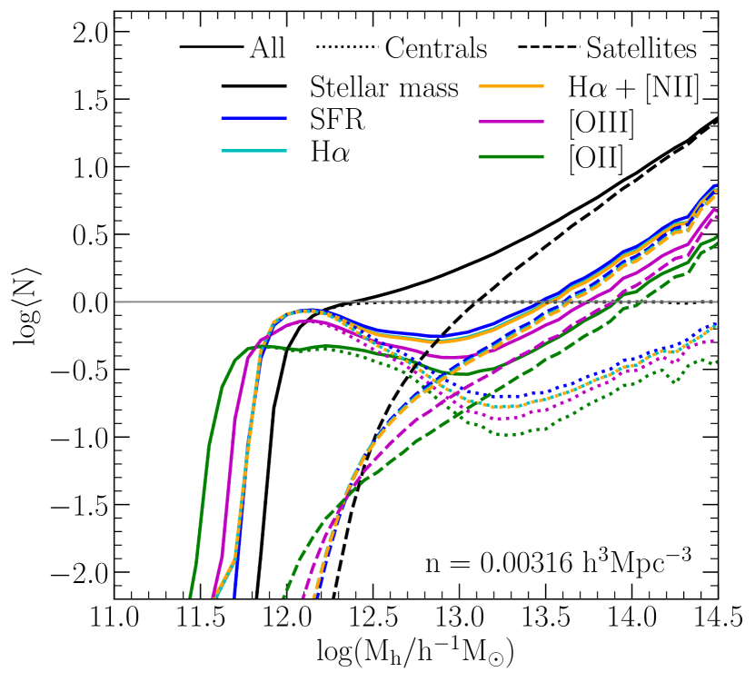
Figure 3: The HODs predicted by the SAG model for all galaxies (solid), centrals (dotted) and satellites (dashed), with different colours indicating different galaxy selections, as shown by the figure key. All samples have a number density of $n=0.00316\ h^{3}{\rm Mpc^{-3}}$.

The overlap between the SFR and ELG-selected samples can be quantified by analysing the similarities in their galaxy properties. Fig. 4 shows the distribution of galaxies in the instantaneous SFR vs. gas metallicity plane for the SFR, H$\alpha$ and [OII] selections, in all cases with a number density $n=0.00316\ h^{3}{\rm Mpc^{-3}}$. As can be seen, the distribution of the H$\alpha$ selected sample is in very good agreement with that of the SFR selection, as expected. In contrast, the distribution for the [OII]-selected sample is shifted to lower instantaneous SFR and cold gas metallicity. Still, an important fraction of [OII] emitters overlap with the SFR and H$\alpha$ selections. Table 1 shows the fraction of overlap between the ELG and SFR selections. Note that ELG and SFR selected samples have less overlap at lower number densities.

$n/h^{3}\rm Mpc^{-3}$	$\rm H\alpha$	$\rm[OIII]$	$\rm[OII]$
$\rm 0.001$	$0.81$	$0.57$	$0.39$
$\rm 0.00316$	$0.91$	$0.71$	$0.47$
$\rm 0.01$	$0.96$	$0.91$	$0.79$

Table 1: Fraction of SFR-selected galaxies that also satisfy the ELG selection criteria. Different rows indicate the number density of the samples as shown in the first column. Columns 2, 3 and 4 give the fraction of objects that also meet the H$\alpha$, [OIII] and [OII] selections, respectively.

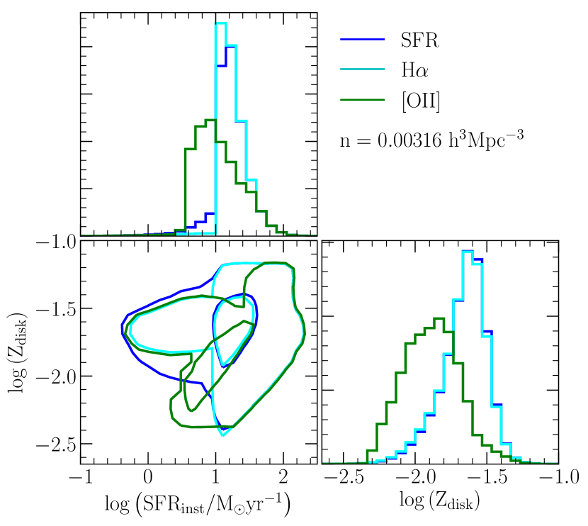
Figure 4: Distributions of instantaneous SFR ($\rm SFR_{inst}$) and cold gas metallicity of the disk ($\rm Z_{disk}$) for SAG samples with fixed number density $n=0.00316\ h^{3}{\rm Mpc^{-3}}$. Different colours correspond to different selections as shown by the key; the density contours enclose 68% and 99% of the distribution of galaxies. The corner panel shows the bivariate distributions, whereas the top and right panels show the marginalised distributions of instantaneous SFR and cold gas metallicity, respectively.

4 The galaxy assembly bias of ELG samples

Measurements from N-body simulations have shown that in order to fully determine the clustering of dark matter haloes one needs, in addition to their masses, knowledge of secondary halo properties such as formation time, concentration, subhalo occupation and spin (e.g Gao et al., 2005; Wechsler et al., 2006; Gao & White, 2007). This effect, termed halo assembly bias, may potentially have an impact on the galaxy content of haloes, producing variations in the halo occupation functions and therefore affecting the large-scale galaxy clustering amplitude (e.g Artale et al., 2018; Zehavi et al., 2018; Contreras et al., 2019). Hence, it is important to model this effect when interpreting the correlation function using the standard HOD framework.

SAM samples that are obtained using halo merger histories extracted from N-body simulations are affected by assembly bias because the growth histories of dark matter haloes, and therefore the level of assembly bias that haloes are subject to, also affect the galaxies that evolve within them. To measure the impact of assembly bias on the clustering of our galaxy samples we compare their 2PCFs with that of “shuffled” galaxy samples. The shuffling removes information about the assembly history of haloes by randomly exchanging the galaxy populations between haloes of the same mass (Croton et al., 2007; Xu et al., 2020). The standard approach preserves the central-satellites distances, therefore the one-halo terms of the shuffled catalogues are the same as those of the original SAM samples. The assembly bias signature can be obtained by comparing the 2PCF of the SAM samples to that of the shuffled samples.

The impact of assembly bias on galaxy clustering depends on the selection criteria, number density and redshift of the sample (e.g Contreras et al., 2019). As the ELG selection shows substantial overlap with selection by SFR (see Fig. 4), we can estimate how much of the effect of assembly bias on the clustering of ELGs comes from the SFR selection. We do this by looking at the assembly bias effect present in a purely SFR-selected sample. Even though nebular emission traces SFR, some properties of the gas in the ISM, such as metallicity, can introduce additional effects that are not included when selecting by SFR alone. The assembly bias signatures for SFR-, stellar mass- and ELG-selected samples are shown in Fig. 5 for the three number densities. It can be seen from Fig. 5 that the assembly bias in the H$\alpha$ and H$\alpha$ + [NII] selections is similar to that seen in the SFR selection. In contrast, assembly bias suppresses the galaxy clustering of [OIII] and [OII] selections by up to $30$ per cent. Table 1 shows that the H$\alpha$ sample has a high overlap with the SFR selected sample for all number densities considered. For [OIII] emitters, the overlap with the SFR-selection is high for the highest number density sample, explaining their similar clustering in the top panel of Fig. LABEL:fig:GAB. For the other number densities considered, the overlap between the [OIII] and SFR selected samples is much smaller and their clustering is different.

Furthermore, the assembly bias is scale-dependent, particularly in the case of [OII]. This steepness in the ratio of the 2PCF to the shuffled samples is also present in the SFR, H$\alpha$ and H$\alpha$+[NII] selections but only for the lowest number densities and, in any case, it is not as scale-dependent as in the [OIII] and [OII] cases. Moreover, there is a “bump" feature in the ratio that is present only for the latter two selections around the transition from the one-halo to the two-halo term ($\log(r/h^{-1}{\rm Mpc})\sim-0.4$). Overall, there is a clear trend between number density and the impact of assembly bias on galaxy clustering; for all ELG selections, the suppression of the clustering amplitude is larger for samples with lower number densities (i.e. for galaxies with higher emission line luminosities). Also, note that the steepness of the assembly bias signature in the [OIII] and [OII] selections is more pronounced for lower number densities. We also show the impact in the stellar mass-selected samples; it can be seen that assembly bias enhances the galaxy clustering and shows no scale-dependence for any of the number densities explored here.

To investigate the origin of the steepness in the assembly bias signature, we analyse the galaxy clustering of the SAG and shuffled samples separately, by comparing their 2PCFs to that of the dark matter. The dark matter 2PCF is obtained from the linear power spectra used in the MDPL2 simulation, which is Fourier transformed to obtain the linear theory matter correlation function. Using the 2PCF of the dark matter, $\xi_{\rm mm}$, and the 2PCF of the galaxy sample $\xi_{\rm gal}$ we compute the large scale bias of each sample using

$$b(r)=\sqrt{\frac{\xi_{\rm gal}}{\xi_{\rm mm}}}.$$ (1)

The value of the bias parameter is expected to be constant to first-order on linear scales and to vary with the galaxy selection.

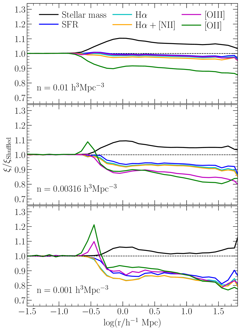
Figure 5: The assembly bias signature in the SAG samples. Each panel shows a different number density as labelled. Note that the assembly bias for the [OIII] and [OII] selections exhibits a clear scale-dependent signature for the two lowest number densities.

The main panels of Fig. 6 show the 2PCFs of the dark matter and the SAG and shuffled samples for the H$\alpha$, [OIII] and [OII] selections, for the number density of $n=0.00316\ h^{3}{\rm Mpc^{-3}}$. For clarity, we show results for the two-halo term only ($\log(r/h^{-1}{\rm Mpc})\gtrsim 0.5$). The estimate of the bias parameter, $b(r)$, for each sample is shown as a coloured line in the bottom panels. We average these values between $25$ and ${\rm 50\ }h^{-1}{\rm Mpc}$ to obtain a constant large-scale bias, which is shown by the gray horizontal lines for comparison with $b(r)$. For the H$\alpha$ selection the bias parameter is roughly constant over the range ${\rm 25<r/}h^{-1}{\rm Mpc\ <50}$, for both the SAG and shuffled samples. In contrast, the bias parameters for the SAG [OIII] and [OII] selections show a scale-dependence. The bias for the shuffled samples is seen to be roughly constant. For the lowest number density sample (not shown here), we find that the bias parameter has an even steeper scale dependence for [OII] and [OIII] selections. The larger value found for the bias of the H$\alpha$ selected sample indicates that, in this case, galaxies trace higher peaks in the density field than galaxies in the other ELG-selected samples.

The prediction of a scale-dependent bias parameter for the SAG [OIII]- and [OII]-selected samples indicates that there are additional features which shape the large scale clustering of these tracers. This suggests that the gas metallicity, which has an impact on the [OII] and [OIII] emission for a given amount of star formation, has some dependence on environment. This is confirmed by the much weaker scale dependence found for the bias on large scales in the shuffled samples.

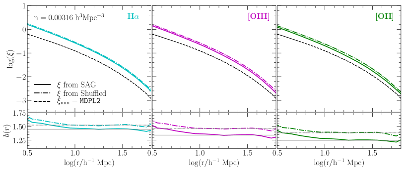
Figure 6: (Top) The 2PCFs of the SAG samples (solid) and the shuffled samples (dashed-dotted) for the H$\alpha$ (left panel), [OIII] (middle panel) and [OII] (right panel) selections. The black dashed lines correspond to the 2PCF of the dark matter distribution of the MDPL2 simulation. (Bottom) The bias parameter, as a function of scale-separation, for the SAG and shuffled samples. The horizontal solid (dashed) grey line corresponds to the bias parameters of the SAG (shuffled) samples averaged between $25$ and $50\ h^{-1}\rm Mpc$.

5 Origin of scale-dependent assembly bias

In this section we investigate the origin of the scale-dependence of the galaxy assembly bias signature in galaxies selected by their [OIII] and [OII] line emission. As just noted, the scale-dependent bias is only present in the original SAG samples and not in their shuffled counterparts. This suggests that the preference for the environment that characterises galaxies with strong line emission, that could cause this scale dependence, is removed when shuffling these samples. Gonzalez-Perez et al. (2020) analyzed how model ELGs trace the large scale structure in an N-Body simulation. They found that about half of [OII] emitters live in filaments while one-third live in sheets. This indicates that the galaxies selected using [OII] line luminosity will be preferentially located in low density regions. Hence, quantifying the effect that the shuffling procedure has of moving ELGs to random locations in the cosmic web can provide an insight into the relation between the environment of [OII] emitters and the scale-dependent assembly bias. Whilst there is some overlap between the SFR and [OII] selected samples, the SFR-selected sample shows little sign of scale dependent bias. Hence, the source of the scale dependence is likely to be found in the galaxies that are not in common between the two samples. Indeed, Table 1 shows that the overlap between the SFR and [OII] emitters is less than 50 per cent for the two lowest density samples. This indicates that the origin of the scale dependence is encoded in the selection by [OII] luminosity.

One approach to quantifying the environment of a galaxy sample is to compute the local number density of main haloes around each galaxy. We use the main halos as we associate galaxies with their host dark matter haloes rather than with subhaloes; not all of the satellite galaxies may be associated with a resolved subhalo. We define the number density, $n_{\rm local}$, using the distance to the fifth nearest main halo in the MDPL2 simulation, $r_{5}$, as $n_{\rm local}=5/V(r_{5})$, where $V(r_{5})$ is the volume of a sphere of radius $r=r_{5}$. To count neighbouring haloes we use those with masses $M_{\rm h}>10^{10.8}h^{-1}\rm M_{\odot}$ for all galaxy selections.

We now consider the contribution of different halos to the sample bias and their environment. Following Kim et al. (2009), we compute the effective clustering bias as a function of halo mass for each galaxy sample, and show the results in the top panel of Fig 7. This parameter quantifies the contribution of galaxies in haloes of a given mass to the large scale galaxy clustering amplitude of the sample. The effective bias is simply computed as $b(M)\times\Phi(M)\times\left<N(M)\right>$ where $b(M)$ is the bias function, $\Phi(M)$ is the halo mass function and $\left<N(M)\right>$ is the halo occupation function of the galaxy sample. For each selection, the effective bias reaches a peak at different halo masses, close to the location of the “knee" of the occupation function (i.e. when the highest fraction of haloes of a given mass contain a central). The middle panel shows the average $n_{\rm local}$ for the SAG and shuffled samples; the bottom panel shows the ratios between the $n_{\rm local}$ of the SAG and shuffled samples for each galaxy selection. Note that a ratio higher than unity indicates that galaxies in the SAG samples are in higher density regions than their shuffled counterparts.

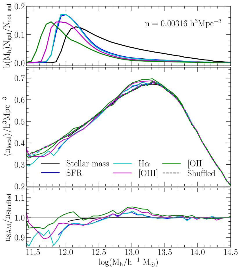
Figure 7: (Top) The contribution to the effective clustering bias from halos as a function of halo mass. (Middle) the average local number densities for the SAG samples (solid) and their shuffled samples (dashed) as a function of halo mass, defined as described in the text. (Bottom) The ratio between the SAG and shuffled density measurements. Different colours indicate different galaxy selections as labelled in the middle panel.

The SAG galaxy samples exhibit different average $n_{\rm local}$, which suggest that these different galaxy populations live in different environments. In contrast, the averaged $n_{\rm local}$ for the shuffled samples are largely the same for all selections. Therefore, it appears that the shuffling procedure removes correlations between the selection and environment. For example, for the [OII]-selected galaxies from SAG, the shuffling removes the strong environmental preference for [OII] emitters to reside in filaments and sheets. As the shuffling procedure moves galaxies between haloes of the same mass, the resulting HODs of the shuffled samples are similar to those of their SAG counterparts, which in turn are notably different between selections (see Fig. 3). Thus, their $b(M)$ and 2PFCs are also different even when their averaged $n_{\rm local}$ are similar. For the stellar mass-selected sample, we see that the ratio of $n_{\rm local}$ in the SAG model to that in the shuffled counterpart is close to unity which indicates that the shuffling procedure does not modify the environment for this particular selection. For the SFR- and ELG-selected samples, on the other hand, the ratios in the bottom panel of Fig. 7 show clear departures from unity. Moreover, these ratios depend on halo mass, which suggests that the mass of the host haloes is related to the strength of the environmental selection of SAG galaxies. Even though all selections show this dependence on mass, in principle, its impact on galaxy clustering only appears to be important when this dependence is seen at halo masses around the peak of the contribution to the effective clustering bias for each selection. In particular, for the [OII] selection, there is an overlap between the peak of the effective bias and the mass dependence of the density ratio in the halo mass range $11.6<\log(M_{\rm h}/h^{-1}{\rm M_{\odot}})<12$. In contrast, for the SFR and H$\alpha$ selections, we find no dependence on halo mass around the peak of the effective bias in $\log(M_{\rm h}/h^{-1}{\rm M_{\odot}})\sim 12$. For the [OIII]-selected sample, the ratio also depends on halo mass but in a narrower range ${\rm 11.7<\log(M_{h}/}h^{-1}{\rm M_{\odot}})<11.9$, which is close to the peak of the effective bias.

Another approach to explore the origin of the scale-dependent assembly bias signature is to analyse the distribution of the gas-phase metallicity in the SAG samples. As the GET_EMLINES code uses this property as an input to predict the [OIII] and [OII] emission line luminosities, we expect that it is correlated to some extent with the spatial distribution of the [OIII] and [OII] selections. Fig. 8 shows the distributions of SAG galaxies in the stellar mass-L[OII] and L(H$\alpha$)-L[OII] planes. The points are colour-coded by metallicity averaged weighting by the mass of cold gas in both disks and bulges. We divide the galaxies into four subsamples separated by cuts in stellar mass, L(H$\alpha$) and L[OII] (dashed lines) that correspond to a number density $n=0.00316\ h^{3}{\rm Mpc^{-3}}$. Galaxies to the right (above) of the vertical (horizontal) dashed lines are contained in the [OII]-selected sample (stellar mass and H$\alpha$ selections). In this way, the overlap between the galaxy samples can be easily seen; for the L(H$\alpha$)-L[OII] plane we see that about half of [OII]-selected galaxies are contained in the H$\alpha$ selection, while for the stellar mass-L[OII] comparison, the [OII] emitters account for 25 per cent of galaxies in the stellar mass selection. Moreover, galaxies in the [OII] selection tend to be more metal-poor than for their H$\alpha$ or stellar mass counterparts, which is consistent with the metallicity distributions in Fig. 4. Indeed, it is clear that a large fraction of the [OII]-selected galaxies, in the bottom-right sectors, are the most metal poor.

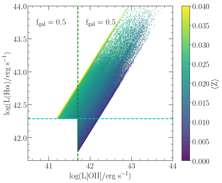
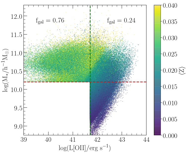
Figure 8: (Left) The H$\alpha$ emission as a function of [OII] emission colour-coded by the cold mass-weighted metallicity of the disks and bulges. The cyan (green) dashed line indicates the cut in H$\alpha$ ([OII]) for a sample of number density $n=0.00316\ h^{3}{\rm Mpc^{-3}}$. The fraction of galaxies with [OII] emission below and above the [OII] cut are included in both sectors. (Right) Same as the left but for stellar mass as a function of [OII] emission.

We compute the auto-correlation functions of galaxies in each sector of the stellar mass-L[OII] plane to look for interesting features in their spatial clustering. We apply the shuffling procedure to these subsamples and measure the 2PCF of the resulting shuffled samples. We also compute the ratios of the 2PCF measured from the SAG subsamples to those of their shuffled counterparts to obtain the assembly bias signatures. The top right panel in Fig. 9 shows the assembly bias signatures for each subsample, colour-coded by its location in the stellar mass-L[OII] plane, as indicated in the left panel. There is a remarkable difference between the assembly bias signatures of the H$\alpha$ subsamples; the red-coded galaxies, which are not included in the [OII] selection, show almost no assembly bias, but the blue-coded ones show a prominent scale-dependence. Moreover, the assembly bias for the grey-coded subsample (which mostly contains metal-poor galaxies), exhibits a steeper dependence on separation. These two results suggest that galaxies with low gas-phase metallicity are driving the scale-dependent assembly bias. To connect this information with the environment of host haloes, we show, in the bottom-right panel of Fig. 9, the distribution of local number densities for galaxies in each subsample. There is a subtle preference for grey-coded galaxies to live in less dense regions than galaxies in the other subsamples. These results suggest that the gas-phase metallicity is the property of the [OIII] and [OII] selections that produces the scale-dependent assembly bias. Specifically, galaxies with low metallicity, that live in low-density regions, appear to account for most of the scale-dependence. Nevetheless, further studies are needed to fully understand the correlation between metallicity and the spatial distribution of galaxies.

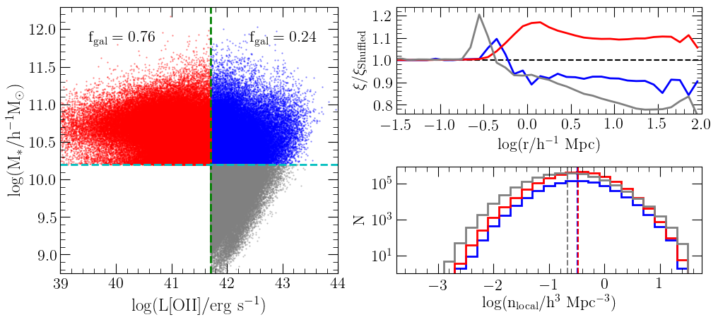
Figure 9: (Left) Same as the right panel of Fig. 8 but with galaxies colour-coded by their location in the stellar mass-L[OII] plane. (Top-right) the assembly bias signatures for the three colour-coded subsamples. (Bottom-right) The local density distribution for galaxies in the color-coded subsamples, where dashed vertical lines correspond to the mean of each distribution.

6 Impact on cosmology

In the previous sections we analyzed the scale-dependent assembly bias in the [OIII] and [OII] selected samples and its relation to the gas-phase metallicity and the environment of the galaxies. The scale dependence was found to be driven by low metallicity galaxies in underdense environments. The scale dependence may have important implications for cosmological analyses.

In this section we focus on the baryon acoustic oscillation (BAO) feature and the $\beta$ parameter. These quantities are measured from each of the SAG samples to check if the ELG selection introduces any systematic effects into the inference of cosmological parameters. This analysis is particularly important for the [OIII] and [OII] selections, as they contain particular features such as a non constant bias and a galaxy assembly bias signal driven by the environment of these galaxies.

Fig. 10 shows the 2PCFs of the SAG (top panels) and shuffled samples (bottom panels) for different selection criteria and number densities. Note that, in order to focus on the BAO peak, we display $r^{2}\times\xi(r)$. For comparison, we show the $\rm z\sim 1$ linear theory prediction for the dark matter 2PCF of the MDPL2. The vertical dotted lines mark the position of the BAO peak for the dark matter.

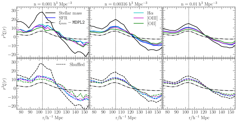
Figure 10: The baryon acoustic oscillation (BAO) feature for the SAG samples (top) and their shuffled counterparts (bottom) with number densities $n=0.001\ h^{3}{\rm Mpc^{-3}}$ (left, $n=0.00316\ h^{3}{\rm Mpc^{-3}}$ (middle) and $n=0.00316\ h^{3}{\rm Mpc^{-3}}$ (right). Colours correspond to the different selections adopted, as shown in the keys. The vertical lines are included to guide the eye and indicate the position of the BAO peak for the dark matter, according to the linear theory prediction (black dot-dashed line).

The amplitudes of the BAO peaks are affected by the large-scale bias of each sample, which depends on the selection criteria, number density and the degree of assembly bias present in the samples (recall the wide range of values found for the large-scale bias for the SAG and shuffled samples in Fig 6). Interestingly, the shape of the BAO peak for the SAG [OII]-selected sample with the intermediate number density (top-middle panel), is notably different with respect to the other samples. The BAO peak position for this selection differs at the $\sim 3$ per cent level from the scale predicted by linear perturbation theory. For the lowest number density, the [OII] selection does not show a clear shift in the BAO scale, although it must be noted that all 2PCFs are somewhat noisy due to the sparsity of this number density. For the highest number density, the BAO scale for the [OII] selection is in agreement with the prediction from linear theory. This result suggests that selecting galaxies with lower [OII] line luminosity washes out the correlation between the [OII] selection and environment (see § 5). Moreover, note that the BAO peak in the [OII] shuffled sample (bottom-middle panel) is not shifted as in the SAG counterpart which suggests that the shuffling procedure removes the shift in the BAO peak. Nevertheless, it is still unclear whether the $\sim 3$ per cent shift would result in a biased measurement of cosmological parameters as the environment effects which influence the clustering measurements for the [OII] sample could also be interpreted as a non-local bias, which can be introduced as a nuisance parameter in BAO peak analyses (e.g. Sánchez et al. 2008).

We also compute the $\beta$ parameter for the SAG samples. This parameter is a function of the logarithmic growth rate, which depends on the matter density parameter, and the bias parameter of the galaxy sample. Following Padilla et al. (2019), we compute $\beta$ for shuffled samples where the relative velocities of the galaxies within haloes – in addition to their positions – are maintained when shuffling satellites between haloes. The $\beta$ parameter can be obtained from the ratio between the monopoles of the correlation functions in real and redshift space (Kaiser, 1986b):

$$\xi_{0}(s)=\left(1+\frac{2}{3}\beta+\frac{1}{5}\beta^{2}\right)\xi(r).$$ (2)

The main panel of Fig. 11 shows the $\beta$ parameter, calculated from Eq. 2, as a function of scale for the SAG (solid) and shuffled samples (dashed) with a number density of $n=0.00316\ h^{3}{\rm Mpc^{-3}}$. For the SAG samples, we see that the $\beta$ parameter is roughly constant for the stellar mass selection, and it is scale-dependent for the other selections. However, for the shuffled samples, the scale dependence of $\beta$ remains. The bottom panel of Fig. 11 shows the ratios between the $\beta$ parameter of the SAG samples to that of their shuffled counterparts. For the stellar mass selection, the ratio is almost constant for all scales. For SFR- and ELG-selected samples, the ratio is more affected by noise, but it appears to be consistent with a constant value, with the SFR and ELG selected samples returning a higher value of beta than their shuffled counterparts. In principle, the steepness of $\beta$ could be so slight that it falls below our noise level, even though we do find a scale-dependent bias for the ELG SAG samples, and a roughly constant one for the shuffled catalogues, especially for the [OIII] and [OII] selections (see Fig. 6).

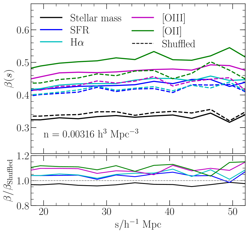
Figure 11: (Top) The $\beta$ parameter as a function of separation for the SAG (solid) and shuffled samples (dotted) with number density $n=0.00316\ h^{3}{\rm Mpc^{-3}}$. Different colours correspond to different selection criteria as indicated by the keys. (Bottom) the ratio between the $\beta$ parameters of the SAG and shuffled samples. The gray dashed line indicates unit ratio.

7 Conclusions

The next generation of galaxy surveys such as DESI and Euclid will map the sky by measuring redshifts to unprecedented numbers of emission-line galaxies. To fully exploit this upcoming data we need to understand how these galaxies trace the underlying density of the Universe and to establish if there are any systematic effects which might impair our ability to extract unbiased cosmological information.

To investigate the potential of ELGs to constrain cosmological parameters, we study the clustering and halo occupation of the model galaxies from the SAG semi-analytical model (Cora et al., 2018) applied to the MDPL2 simulation outputs (Klypin et al., 2016). We use the instantaneous SFR and gas-phase metallicities of galaxies as the inputs to the GET_EMLINES code to obtain the nebular line emission of the galaxies. To mimic the selection criteria of future surveys, we use fixed number density samples where galaxies are ranked according to their [OIII], [OII], H$\alpha$ and H$\alpha$+[NII] line luminosities. For comparison, we also include SFR- and stellar mass-selected samples.

We measure the two-point correlation functions (2PCFs), the halo occupation distributions (HODs) and the galaxy assembly bias signatures for each galaxy sample. The galaxy assembly bias is measured via the ratio between the 2PCF of a SAG sample with that of a shuffled version of the sample, which, by construction, does not contain assembly bias. We also compute the absolute large scale bias of ELGs to look for correlations between assembly bias, large-scale bias, the environment of the galaxies, and the gas-phase metallicity of the ELG-selected samples. Finally, we measure the BAO feature and the $\beta$ parameter for the SAG and shuffled samples to investigate the implications for cosmological studies using ELGs. Our results can be summarised as follows:

• ELG-selected samples have 2PCFs and HODs that are similar to those of SFR selected galaxies. However, the [OIII]- and [OII]-selected samples are less clustered than either the SFR or H$\alpha$ samples. Moreover, their HODs indicate that most of the selected galaxies live in low mass haloes. These differences explain why selecting by the luminosity of the [OIII] or [OII] lines does not reproduce the behaviour of a SFR selected sample.

• The assembly bias signature (i.e. the ratio between the 2PCFs measured for the SAG and shuffled samples) for the [OIII] and [OII] selected samples is scale-dependent, with a steepness which becomes more pronounced for lower density samples (higher [OIII] and [OII] thresholds). For the SFR and H$\alpha$ selections, the assembly bias is scale-dependent for samples with the lowest number density. In the case of galaxies selected by stellar mass, the assembly bias is roughly constant for all number densities.

• The large-scale bias, defined as the ratio between the 2PCF of a galaxy sample and that of the dark matter, is scale-dependent for the [OIII]- and [OII]-selected samples in the SAG model. For the shuffled samples, in contrast, the large-scale bias is roughly constant for all selections. This suggests that the shuffling procedure removes an encoded dependence between the galaxy properties of [OIII] and [OII] selections with the environment.

• For a fixed halo mass the local number density - that we use to quantify the environment of host haloes - is roughly the same for all shuffled samples. This indicates that the shuffling procedure eliminates the correlation between the selection and the environment of host haloes. In contrast, for the SAG samples the local number densities are notably different between the selection criteria which indicates that in some cases the selected galaxies live in special regions of the cosmic web. Moreover, the change of the environment of the [OII]-selected sample has a strong dependence with halo mass (see Fig. 7).

• Galaxies with low gas-phase metallicities are the ones that produce the scale-dependent assembly bias signature. Indeed, for the SAG sample, a larger fraction of metal-poor galaxies results in a steeper scale-dependent assembly bias signature (see Fig. 9). Moreover, these galaxies tend to live in low-density regions, which is more common for the ELG selected samples.

• The scale of the BAO feature in the [OII]-selected sample with number density $n=0.00316\ h^{3}{\rm Mpc^{-3}}$, differs at the 3 per cent level from that recovered using the other selections. Interestingly, this shift in the BAO peak is not seen for the shuffled counterpart of the [OII] sample. Conversely, for the other selected samples, the BAO feature is located at the same position for both the SAG and shuffled samples. There is no clear shift in the position of the BAO feature for the [OII] selections with lower and higher number densities.

• The $\beta$ parameter for the SFR- and ELG-selected samples is non-constant as a function of scale for the SAG and the shuffled samples. This is clearer for the [OII] and [OIII] selections and can be explained as a combination of the scale-dependent large scale bias and a possible non-constant logarithmic growth rate. For the stellar mass case, in contrast, $\beta$ is roughly constant.

Our results show that care must be given when using future galaxy samples from Euclid and DESI, which will be selected by their emission line luminosities. We find that this type of selection can produce samples that lie in special environments, and because of this their clustering can show a different slope than that of the underlying matter density field. This type of environment selection needs to be modelled and marginalised over in cosmological parameter constraints from such samples in order to avoid systematic effects in their analysis.

Data availability statement

The data underlying this article will be shared on reasonable request to the corresponding author.

Appendix A Assembly bias of ELGs in L-GALAXIES

To assess if the scale-dependent assembly bias can be found in other semi-analytical models, we select galaxy samples at z=0 from the Guo et al. (2013) model (hereafter G13) which is a version of the L-GALAXIES code from the Munich group (De Lucia et al., 2004; Croton et al., 2006; De Lucia & Blaizot, 2007; Guo et al., 2011; Henriques et al., 2013). G13 is a semi-analytic model, and as such it models a set of physical processes that shape the formation and evolution of galaxies, applied to halo merger trees drawn from the Millennium-WMAP7 simulation. This simulation was carried out in a box of 500 $h^{-1}$ Mpc a side, and is the same as the original Millennium simulation (Springel et al., 2005) but with updated cosmological parameters that match the results from the WMAP7 observations.

We use the GET_EMLINES code to obtain the nebular emission for G13 galaxies. The instantaneous SFR is not a direct output of G13, hence, we use the average SFR instead to infer line emission luminosities. This is motivated by the results of Favole et al. (2020); they demonstrate that using average SFRs as inputs for GET_EMLINES produces good predictions to study average populations of [OII] emission-line galaxies. We then define new stellar mass, SFR, H$\alpha$, [OIII] and [OII] selected samples following the procedure in § 2.4.

Fig. 12 shows the assembly bias signatures for the G13 samples with three different number densities (the same ones used to define the SAG samples). Note that the 2PCFs of the H$\alpha$ and SFR selections are the same, which is a consequence of H$\alpha$ luminosity having a simple dependence on the SFR, with little variation with the cold gas metallicity. Even though the clustering measurements are noisier at very large scales, we still find that the [OIII] and [OII] selections have a clear scale-dependent assembly bias. In contrast, for the SFR and H$\alpha$ selections, the scale-dependence is there for the lowest number density sample alone, while for the stellar mass-selected samples the signature is roughly flat in all cases.

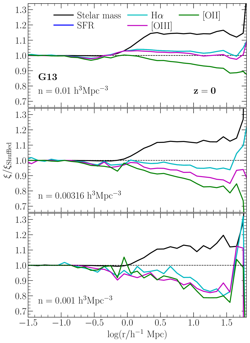
Figure 12: Same as Fig. 5 but for galaxy samples extracted from the Guo et al. (2013) SAM.

Appendix B Completeness of ELG selected samples

Selecting by emission line luminosities produces samples that trace the amplitude of SFR but also other additional properties, such as the cold gas metallicity. Thus, in principle, a low-SFR galaxy may be included in an ELG-selected sample. Because of this we analyze the effect of the moderate stellar mass cut imposed on the SAG data, which is present in the subsamples analyzed in this work; this moderate cut is $M_{*}>10^{8.7}h^{-1}{\rm M_{\odot}}$ which is slightly lower than the resolution of the MDPL2 and Millennium simulations (${\rm\sim 10^{9}}\ h^{-1}{\rm M_{\odot}}$).

As SAG and G13 show similar trends for assembly bias (see Fig. 12), we expect that the effect of the completeness stellar mass cut on these trends should be also similar for both models. Fig. 13 displays the cumulative SFR function for subsamples of G13, defined by different stellar mass cuts. As expected from the stellar mass-SFR relation, we see that the larger the cut, the smaller the number of low-SFR galaxies.

We define a subsample of G13 by selecting galaxies with stellar mass above the cut imposed for SAG. Then, following the procedure in §. 2.4, we define our galaxy samples with this new cut. We measure the assembly bias signatures for these samples, and we compare them with the assembly bias of G13 samples with no previous cuts in stellar mass. We find that the assembly bias signatures are almost identical for all selections and number densities. Noticeable differences only arise at very large scales(${\rm\log(r/h^{-1}\ Mpc)>1.5}$). This indicates that the moderate stellar mass cut introduced to impose completeness has only a minor impact on the assembly bias signature, which includes the scale-dependence for [OIII] and [OII] selections.

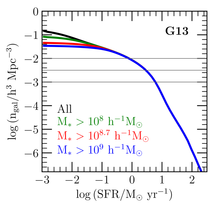
Figure 13: The cumulative SFR function of subsamples of the Guo et al. (2013) model defined by different stellar mass cuts indicated by the colors and labels. Horizontal lines indicate the different number densities used to define the galaxy samples.

References

- Artale et al. (2018) Artale M. C., Zehavi I., Contreras S., Norberg P., 2018, MNRAS, 480, 3978
- Baldwin et al. (1981) Baldwin J. A., Phillips M. M., Terlevich R., 1981, PASP, 93, 5
- Baugh (2006) Baugh C. M., 2006, Reports on Progress in Physics, 69, 3101
- Baugh et al. (2019) Baugh C. M., et al., 2019, MNRAS, 483, 4922
- Bautista et al. (2018) Bautista J. E., et al., 2018, ApJ, 863, 110
- Behroozi et al. (2013a) Behroozi P. S., Wechsler R. H., Wu H.-Y., 2013a, ApJ, 762, 109
- Behroozi et al. (2013b) Behroozi P. S., Wechsler R. H., Wu H.-Y., Busha M. T., Klypin A. A., Primack J. R., 2013b, ApJ, 763, 18
- Benson (2012) Benson A. J., 2012, New Astron., 17, 175
- Benson et al. (2000) Benson A. J., Cole S., Frenk C. S., Baugh C. M., Lacey C. G., 2000, MNRAS, 311, 793
- Berlind & Weinberg (2002) Berlind A. A., Weinberg D. H., 2002, ApJ, 575, 587
- Byler et al. (2017) Byler N., Dalcanton J. J., Conroy C., Johnson B. D., 2017, ApJ, 840, 44
- Cole et al. (2000) Cole S., Lacey C. G., Baugh C. M., Frenk C. S., 2000, MNRAS, 319, 168
- Cole et al. (2005) Cole S., et al., 2005, MNRAS, 362, 505
- Contreras et al. (2013) Contreras S., Baugh C. M., Norberg P., Padilla N., 2013, MNRAS, 432, 2717
- Contreras et al. (2019) Contreras S., Zehavi I., Padilla N., Baugh C. M., Jiménez E., Lacerna I., 2019, MNRAS, 484, 1133
- Contreras et al. (2020) Contreras S., Angulo R., Zennaro M., 2020, arXiv e-prints, p. arXiv:2005.03672
- Cora (2006) Cora S. A., 2006, MNRAS, 368, 1540
- Cora et al. (2018) Cora S. A., et al., 2018, MNRAS, 479, 2
- Croton et al. (2006) Croton D. J., et al., 2006, MNRAS, 365, 11
- Croton et al. (2007) Croton D. J., Gao L., White S. D. M., 2007, MNRAS, 374, 1303
- Croton et al. (2016) Croton D. J., et al., 2016, ApJS, 222, 22
- DESI Collaboration et al. (2016) DESI Collaboration et al., 2016, arXiv e-prints, p. arXiv:1611.00036
- Dawson et al. (2013) Dawson K. S., et al., 2013, AJ, 145, 10
- Dawson et al. (2016) Dawson K. S., et al., 2016, AJ, 151, 44
- De Lucia & Blaizot (2007) De Lucia G., Blaizot J., 2007, MNRAS, 375, 2
- De Lucia et al. (2004) De Lucia G., Kauffmann G., White S. D. M., 2004, MNRAS, 349, 1101
- Dopita & Sutherland (1995) Dopita M. A., Sutherland R. S., 1995, ApJ, 455, 468
- Eisenstein et al. (2005) Eisenstein D. J., et al., 2005, ApJ, 633, 560
- Eisenstein et al. (2011) Eisenstein D. J., et al., 2011, AJ, 142, 72
- Favole et al. (2016) Favole G., et al., 2016, MNRAS, 461, 3421
- Favole et al. (2020) Favole G., et al., 2020, MNRAS,
- Gao & White (2007) Gao L., White S. D. M., 2007, MNRAS, 377, L5
- Gao et al. (2005) Gao L., Springel V., White S. D. M., 2005, MNRAS, 363, L66
- Gargiulo et al. (2015) Gargiulo I. D., et al., 2015, MNRAS, 446, 3820
- Gonzalez-Perez et al. (2018) Gonzalez-Perez V., et al., 2018, MNRAS, 474, 4024
- Gonzalez-Perez et al. (2020) Gonzalez-Perez V., et al., 2020, arXiv e-prints, p. arXiv:2001.06560
- Groves & Allen (2010) Groves B. A., Allen M. G., 2010, New Astron., 15, 614
- Groves et al. (2004) Groves B. A., Dopita M. A., Sutherland R. S., 2004, ApJS, 153, 9
- Guo et al. (2011) Guo Q., et al., 2011, MNRAS, 413, 101
- Guo et al. (2013) Guo Q., White S., Angulo R. E., Henriques B., Lemson G., Boylan-Kolchin M., Thomas P., Short C., 2013, MNRAS, 428, 1351
- Gutkin et al. (2016) Gutkin J., Charlot S., Bruzual G., 2016, MNRAS, 462, 1757
- Henriques et al. (2013) Henriques B. M. B., White S. D. M., Thomas P. A., Angulo R. E., Guo Q., Lemson G., Springel V., 2013, MNRAS, 431, 3373
- Henriques et al. (2015) Henriques B. M. B., White S. D. M., Thomas P. A., Angulo R., Guo Q., Lemson G., Springel V., Overzier R., 2015, MNRAS, 451, 2663
- Jiménez et al. (2019) Jiménez E., Contreras S., Padilla N., Zehavi I., Baugh C. M., Gonzalez-Perez V., 2019, MNRAS, 490, 3532
- Kaiser (1986a) Kaiser N., 1986a, MNRAS, 219, 785
- Kaiser (1986b) Kaiser N., 1986b, MNRAS, 222, 323
- Kim et al. (2009) Kim H.-S., Baugh C. M., Cole S., Frenk C. S., Benson A. J., 2009, MNRAS, 400, 1527
- Klypin et al. (2016) Klypin A., Yepes G., Gottlöber S., Prada F., Heß S., 2016, MNRAS, 457, 4340
- Knebe et al. (2018) Knebe A., et al., 2018, MNRAS, 474, 5206
- Kravtsov et al. (2004) Kravtsov A. V., Berlind A. A., Wechsler R. H., Klypin A. A., Gottlöber S., Allgood B., Primack J. R., 2004, ApJ, 609, 35
- Lagos et al. (2008) Lagos C. D. P., Cora S. A., Padilla N. D., 2008, MNRAS, 388, 587
- Lagos et al. (2018) Lagos C. d. P., Tobar R. J., Robotham A. S. G., Obreschkow D., Mitchell P. D., Power C., Elahi P. J., 2018, MNRAS, 481, 3573
- Laureijs et al. (2011) Laureijs R., et al., 2011, arXiv e-prints, p. arXiv:1110.3193
- Levesque et al. (2010) Levesque E. M., Kewley L. J., Larson K. L., 2010, AJ, 139, 712
- Merson et al. (2018) Merson A., Wang Y., Benson A., Faisst A., Masters D., Kiessling A., Rhodes J., 2018, MNRAS, 474, 177
- Montero-Dorta et al. (2020) Montero-Dorta A. D., et al., 2020, MNRAS, 496, 1182
- Muñoz Arancibia et al. (2015) Muñoz Arancibia A. M., Navarrete F. P., Padilla N. D., Cora S. A., Gawiser E., Kurczynski P., Ruiz A. N., 2015, MNRAS, 446, 2291
- Nagao et al. (2006) Nagao T., Maiolino R., Marconi A., 2006, A&A, 459, 85
- Nelson et al. (2018) Nelson D., et al., 2018, MNRAS, 475, 624
- Orsi et al. (2014) Orsi Á., Padilla N., Groves B., Cora S., Tecce T., Gargiulo I., Ruiz A., 2014, MNRAS, 443, 799
- Padilla et al. (2014) Padilla N. D., Salazar-Albornoz S., Contreras S., Cora S. A., Ruiz A. N., 2014, MNRAS, 443, 2801
- Padilla et al. (2019) Padilla N., Contreras S., Zehavi I., Baugh C. M., Norberg P., 2019, MNRAS, 486, 582
- Planck Collaboration et al. (2014) Planck Collaboration et al., 2014, A&A, 571, A16
- Ruiz et al. (2015) Ruiz A. N., et al., 2015, ApJ, 801, 139
- Sánchez et al. (2008) Sánchez A. G., Baugh C. M., Angulo R. E., 2008, MNRAS, 390, 1470
- Schaye et al. (2015) Schaye J., et al., 2015, MNRAS, 446, 521
- Scoccimarro et al. (2001) Scoccimarro R., Feldman H. A., Fry J. N., Frieman J. A., 2001, ApJ, 546, 652
- Shim & Chary (2013) Shim H., Chary R.-R., 2013, ApJ, 765, 26
- Sinha & Garrison (2017) Sinha M., Garrison L., 2017, Corrfunc: Blazing fast correlation functions on the CPU, Astrophysics Source Code Library (ascl:1703.003)
- Somerville et al. (2008) Somerville R. S., Hopkins P. F., Cox T. J., Robertson B. E., Hernquist L., 2008, MNRAS, 391, 481
- Springel et al. (2001) Springel V., White S. D. M., Tormen G., Kauffmann G., 2001, MNRAS, 328, 726
- Springel et al. (2005) Springel V., et al., 2005, Nature, 435, 629
- Stevens et al. (2016) Stevens A. R. H., Croton D. J., Mutch S. J., 2016, MNRAS, 461, 859
- Tecce et al. (2010) Tecce T. E., Cora S. A., Tissera P. B., Abadi M. G., Lagos C. D. P., 2010, MNRAS, 408, 2008
- Vogelsberger et al. (2014) Vogelsberger M., et al., 2014, MNRAS, 444, 1518
- Wechsler & Tinker (2018) Wechsler R. H., Tinker J. L., 2018, ARA&A, 56, 435
- Wechsler et al. (2006) Wechsler R. H., Zentner A. R., Bullock J. S., Kravtsov A. V., Allgood B., 2006, ApJ, 652, 71
- Weinberg et al. (2013) Weinberg D. H., Mortonson M. J., Eisenstein D. J., Hirata C., Riess A. G., Rozo E., 2013, Phys. Rep., 530, 87
- Xu & Zheng (2020) Xu X., Zheng Z., 2020, MNRAS, 492, 2739
- Xu et al. (2020) Xu X., Zehavi I., Contreras S., 2020, arXiv e-prints, p. arXiv:2007.05545
- Zehavi et al. (2011) Zehavi I., et al., 2011, ApJ, 736, 59
- Zehavi et al. (2018) Zehavi I., Contreras S., Padilla N., Smith N. J., Baugh C. M., Norberg P., 2018, ApJ, 853, 84
- Zehavi et al. (2019) Zehavi I., Kerby S. E., Contreras S., Jiménez E., Padilla N., Baugh C. M., 2019, ApJ, 887, 17
- Zheng et al. (2005) Zheng Z., et al., 2005, ApJ, 633, 791