Recursion relation for instanton counting for $SU(2)$ ${\cal N}=2$ SYM in NS limit of $\Omega$ background

Abstract

In this paper we investigate different ways of deriving the A-cycle period as a series in instanton counting parameter $q$ for ${\cal N}=2$ SYM with up to four antifundamental hypermultiplets in NS limit of $\Omega$ background. We propose a new recursive method for calculating the period and demonstrate its efficiency by explicit calculations. The new way of doing instanton counting is more advantageous compared to known standard techniques and allows to reach substantially higher order terms with less effort. This approach is applied for the pure case as well as for the case with several hypermultiplets.

In addition we suggest a numerical method for deriving the $A$-cycle period for arbitrary values of $q$. In the case when one has no hypermultiplets for the A-cycle an analytic expression for large $q$ asymptotics is obtained using a conjecture by Alexei Zamolodchikov. We demonstrate that this expression is in convincing agreement with the numerical approach.

1 Introduction

The focus of this paper is the A-cycle period for the ${\cal N}=2$ SYM with gauge group $SU(2)$ in $\Omega$ background (see Lossev:1997bz ; Nekrasov:2002qd and further developments Flume:2002az ; Nekrasov:2003rj ; Bruzzo:2002xf ). The background is parameterized by two parameters $\epsilon_{1}$ and $\epsilon_{2}$ which can be interpreted as angular velocities on two orthogonal planes of the space time. We will be interested in the case when one of the parameters say $\epsilon_{2}$ is sent to zero while the other one is kept finite, commonly referred as Nekrasov-Shatashvili (NS) limit Nekrasov:2009rc .

According to the AGT relation Alday:2009aq the instanton partition function in $\Omega$ background is closely related to the conformal block of $2d$ Liouville CFT. Thus any result related to the partition function can be reinterpreted in terms of the conformal block and vice versa. The NS limit corresponds to the so called heavy classical limit of the conformal block Seiberg:1990eb ; Zamolodchikov:1995aa . The four point conformal block satisfies a well known recursion relation discovered by Alexei Zamolodchikov Zamolodchikov:1984aj ; Zamolodchikov:1987aj (for the analog in gauge theory side see Poghossian:2009mk and for generalizations of CFT see Poghossian:2017atl ; Hadasz:2006qb ; Hadasz:2008dt ). Surely, Zamolodchikov’s recursion relation may be explored to investigate the heavy conformal block, by computing first the exact block and only afterwords tacking the heavy limit. Nevertheless this procedure appears to be rather inefficient. Meanwhile constructing a heavy analog of Zamolodchikov’s recursion relation directly is not straightforward, due to arising strong singularities Alekseev:2019gkl ; Beccaria:2016wop ; Gorsky:2017ndg . A natural question is whether a kind of alternative procedure, efficiently working in heavy limit, can be found. The current article provides a positive answer to this question.

The method we suggest is the following: the Nekrasov partition function can be represented as a sum over pairs of ($N$-tuples if the gauge group is $U(N)$) Young diagrams Nekrasov:2002qd ; Flume:2002az . In NS limit only a single term of this sum contributes dominantly. A major role is played by an entire function whose zeros are determined by the column length of dominant Young diagrams mentioned above. This function satisfies a difference equation Poghossian:2010pn , which can be reformulated in such a way that it closely resembles the ordinary Seiberg–Witten curve equation Seiberg:1994rs ; Seiberg:1994aj . We have made use of this difference equation to obtain a recursion relation in terms of continued fractions.

To demonstrate the simplicity of our approach we compere it with two other well known methods. One of which is by making use of the combinatorial formula for the instanton partition function and the other one performing contour integration of the deformed SW differential and using generalized Matone relation Flume:2004rp . Another well known way of deriving the A-cycle is with the help of the holomorphic anomaly equations Huang:2011qx ; Huang:2014nwa . Although the result by this approach has the advantage of giving exact expressions in instanton parameter $q$ but now it is a series in $\epsilon$.

In this paper we also investigate a numerical approach to derive the A-cycle period again directly applicable in NS limit. Via Fourier transform from the already mentioned difference equation a second order ordinary differential equation (ODE) can be derived Fucito:2011pn (for earlier works using different approach see Mironov:2009uv ; Mironov:2009dv ; Maruyoshi:2010iu ). Since the coefficients entering in this differential equation are periodic one deduces that it admits quasi-periodic solutions. The index of quasi periodicity or the characteristic exponent commonly referred as Floquet exponent is just the A-cycle period. In particular when one considers pure $SU(2)$ SYM the differential equation is just the (modified) Mathieu equation which is well studied in mathematical literature (for example see NIST:DLMF ). The fact that it can serve as a basis for numerical computations is emphasized in Zamolodchikov:2000unpb ; Fioravanti:2019awr . In this work we demonstrate how the corresponding differential equations for $SU(2)$ SYM with several hypermultiplets can be used for numerical computations in similar manner. In particular in the case when one has four hypers, due to the AGT correspondence, this numerical approach can be used to investigate the heavy conformal block.

There was recent progress in generalizing the SW curve for generic $\Omega$-background too Nekrasov:2015wsu ; Poghosyan:2016mkh ; Poghosyan:2018sae . Extension of our analyses is an interesting task, though beyond the scope of the current paper. The numerical approach via the monodromy matrix is applicable for the case of $N=2^{*}$ too but the analog for our recursion relation here is not clear since in this case the difference equation is of infinite order Fucito:2011pn ; Nekrasov:2013xda .

Using results of Zamolodchikov:2000unpb we derive an analytic expression for $a(q)$ for large values of instanton counting parameter $q$ and check its validity by numerical computations. This is achieved only for the pure case and it would be interesting to find analogous expressions in the presence of matter hypermultiplets.

This article is organized as follows: section 2 we review few known things connected to instanton counting and the A-cycle period to make clear the notations we used. In section 3 we give our recursion relation for pure SYM. A numerical approach is presented in subsections 3.2, 3.3 which is applied to investigate the A-cycle in $SU(2)$ SYM. This numerical method was previously used in Zamolodchikov:2000unpb to investigate the Floquet exponent in the context of Ordinary Differential Equation/Integrable Model (ODE/IM) correspondence Dorey:1998pt ; Bazhanov:1998wj and also for $SU(3)$ pure SYM Fioravanti:2019awr . We show that results obtained by this numerical method are consistent with our recursion relation. In addition we derive an analytic formula for $a(q)$ valid in large $q$ limit. The latter is achieved with the help of a conjecture about the Floquet exponent of Mathieu equation Zamolodchikov:2000unpb ; Zamolodchikov:2000kt . We end section 3 by checking the asymptotic formula for $a(q)$ numerically. In section 4 we extend previous results to the case with hypermultiplets. Equation (59) expresses our recursion relation for arbitrary number of hypermultiplets. Using our new recursive method in final section 5 we compute the heavy conformal block as a series in cross ratio of insertion points.

2 A brief review of instanton counting and A-cycle period

In this section we briefly review the combinatorial expression for instanton partition function, the difference relation emerging in NS limit and define the period cycles. Connection between the differences relation and generalized SW curve is explained. We discus some of the similarities and differences between the ordinary SW curve and its generalization for NS limit of $\Omega$ background. The A-period computation is performed using two approaches, first, using instanton counting combined with Matone relation and the second by integrating deformed SW differential.

2.1 The deformed prepotential in the NS limit

Consider ${\cal N}=2$ SYM with gauge group $SU(2)$ and four hypermultiplets in $\Omega$-background parameterized by $\epsilon_{1}$ and $\epsilon_{2}$. The instanton part of the partition function Nekrasov:2002qd of this theory can be represented as Flume:2002az ; Bruzzo:2002xf

$$Z_{inst}(a,\epsilon_{1},\epsilon_{2},q)=\sum_{\vec{Y}}\frac{Z_{f}(\vec{Y})}{Z_{g}(\vec{Y})}q^{|\vec{Y}|},$$ (1)

where $\vec{Y}$ is a pair of Young diagrams $\vec{Y}=(Y_{1},Y_{2})$ and $|\vec{Y}|$ is the total number of boxes. The sum is over all possible pairs of Young diagrams and $q$ is the instanton counting parameter related to the gauge coupling $g$ and the CP violating parameter $\theta$ in the standard manner: $q=\exp(2\pi i\tau)$, with $\tau=\frac{i}{g^{2}}+\frac{\theta}{2\pi}$. We denote the VEV of adjoint scalar of ${\cal N}=2$ vector multiplet by $a_{1}=-a_{2}=a$. The contribution of antifundamental hypermultiplets $Z_{f}$ and the gauge multiplet $Z_{g}$ can be represented as Flume:2002az ; Bruzzo:2002xf

$$Z_{f}(\vec{Y}) = \prod_{\ell=1}^{N_{f}}\prod_{u=1}^{2}\prod_{(i,j)\in Y_{u}}\left(m_{\ell}+a_{u}+(i-1)\epsilon_{1}+(j-1)\epsilon_{2}\right)\,,$$ (2)

$$Z_{g}(\vec{Y}) = \prod_{u,v=1}^{2}\displaystyle\prod_{s\in Y_{u}}\big{(}a_{u}-a_{v}-\epsilon_{1}L_{\mu}(s)+\epsilon_{2}(1+A_{\lambda}(s))\big{)}\times$$

$$\quad\,\,\times\,\displaystyle\prod_{s\in Y_{v}}\big{(}a_{u}-a_{v}+\epsilon_{1}(1+L_{\lambda}(s))-\epsilon_{2}A_{\mu}(s)\big{)}\,.$$

Here by $m_{\ell}$ we denote the masses of the hypermultiplets, $A_{\lambda}(s)$ and $L_{\lambda}(s)$ are the arm-length and leg-length of the box $s$ with respect to the Young diagram $\lambda$ respectively. The arm-length $A_{\lambda}(s)$ (leg-length $L_{\lambda}(s)$) is the number of steps needed to reach from the box $s$ to the outer boundary of $\lambda$ in vertical (horizontal) direction as demonstrated in Fig.1. The coordinates $(i,j)$ in (2.1) specify the position of a box (see Fig.1).

Figure 1: Arm and leg length with respect to the Young diagram whose borders are outlined by dark black: $A(s_{1})=-2$, $L(s_{1})=-2$, $A(s_{2})=2$, $L(s_{2})=3$, $A(s_{3})=-3$, $L(s_{3})=-4$. The coordinate $(i,j)$ of the box $s_{2}$ is $(3,1)$.

The deformed prepotential in the NS limit is defined as

$$F_{inst}(a,\epsilon_{1},q)=-\lim\limits_{\epsilon_{2}\to 0}\epsilon_{1}\epsilon_{2}\log Z_{inst}(a,\epsilon_{1},\epsilon_{2},q)\,.$$ (4)

From here on the notation $\epsilon_{1}\equiv\epsilon$ will be used. We will need also the Matone relation Matone:1995rx

$$u=\langle{\rm tr\phi^{2}}\rangle=2a^{2}+2q\frac{\partial F_{inst}}{\partial q}=2q\frac{\partial F}{\partial q}\,,$$ (5)

which holds also in the presence of $\Omega$ background Flume:2004rp . With the help of this expressions one can derive the A-cycle period as a power series in $q$ (see appendix B.2 for explicit calculations). Most of the time instead of the VEV parameter $u$ we will us the parameter $p$ defined as

$$p^{2}\equiv\frac{u}{2}=\frac{\langle{\rm tr\phi^{2}}\rangle}{2}\,.$$ (6)

2.2 The difference equation and the SW curve equation

According to Poghossian:2010pn the sum (1) in NS limit is dominated by a single term corresponding to a unique pair of Young diagrams $\vec{Y}^{(cr)}$. By using this fact one defines an entire function $Y(z)$ whose zeros $z_{u,k}$ are determined by (rescaled) column lengths $\lambda_{u,k}$ of $\vec{Y}^{(cr)}$:

$$z_{u,k}=a_{u}+(k-1)\epsilon+\lambda_{u,k}\,,\quad u=1,2.$$ (7)

For later use we will also need the fact that $\lambda_{u,k}\sim O(q^{k})$. It was shown in Poghossian:2010pn that such function $Y(z)$, if defined properly satisfies the difference equation

$$Y(z+\epsilon)+\epsilon^{-4}Q_{N_{f}}(z+\epsilon)Y(z-\epsilon)=\epsilon^{-2}P_{N_{f}}(z+\epsilon)Y(z)\,.$$ (8)

This difference equation leads to a kind of generalization of the Seiberg-Witten curve equation. Introducing the meromorphic function

$$y(z)=\epsilon^{2}\frac{Y(z)}{Y(z-\epsilon)}\,,$$ (9)

from (8) one immediately gets

$$y(z)+\frac{Q_{N_{f}}(z)}{y(z-\epsilon)}=P_{N_{f}}(z)\,.$$ (10)

In the case $N_{f}=4$ one has

$$Q_{4}(z)=q\prod_{j=1}^{4}(z+m_{j}-\epsilon)\,;$$ (11)

$$P_{4}(z)=(1+q)z^{2}+\left(s_{1}-2\epsilon\right)qz+q\left(s_{2}-\epsilon s_{1}+p^{2}+\epsilon^{2}\right)-p^{2}\,,$$ (12)

where $s_{1}$ and $s_{2}$ are elementary symmetric polynomials of masses

$$s_{1}=\sum_{i=1}^{4}m_{i};\,\,\,s_{2}=\sum_{1\leq i<j\leq 4}m_{i}m_{j};\,\,\,s_{3}=\sum_{1\leq i<j<k\leq 4}m_{i}m_{j}m_{k};\,\,\,s_{4}=m_{1}m_{2}m_{3}m_{4}.$$ (13)

As usual less number of flavors can be obtained from above expressions by sending some of the masses to infinity simultaneously rescaling the instanton parameter appropriately (for details see appendix A). Notice that by setting $\epsilon=0$ in (10) one obtains the usual SW curve equation Seiberg:1994rs ; Seiberg:1994aj presented as in Nekrasov:2003rj

$$y(z)+\frac{Q_{N_{f}}(z)}{y(z)}=P_{N_{f}}(z)\,,$$ (14)

where $y(z)$ is related to Seiberg-Witten differential as

$$\lambda_{SW}=z\frac{d}{dz}\log y(z)\,.$$ (15)

From the curve equation (14)

$$y(z)=\frac{1}{2}\left(P_{N_{f}}(z)+\sqrt{P_{N_{f}}(z)^{2}-4Q_{N_{f}}(z)}\right)\,.$$ (16)

We have chosen the plus sign to ensure the appropriate large $z$ behavior $y(z)\sim z^{2}$. The branch points on $z$ plane can be found from vanishing discriminant condition

$$P_{N_{f}}(z)^{2}-4Q_{N_{f}}(z)=0\,.$$ (17)

Let us denote the roots by $z_{j}$, $j=1,2,3,4$ ordered as $z_{1}<z_{2}<z_{3}<z_{4}$ (here for simplicity we assume that the parameters $m$ and $q$ are real and $q\ll 1$). We choose the branch cuts to be extended from $z_{1}$ to $z_{2}$ and from $z_{3}$ to $z_{4}$ (see Fig.2). The Seiberg-Witten curve is obtain by gluing two Riemann sheets along the cuts.

Figure 2: Branch points and cycles on $z$ plane

The monodromy cycles $a$ and $a_{D}$ are integrals of SW differential (15) along non contractible curves $\mathcal{C}_{A}$, $\mathcal{C}_{B}$ respectively (see Fig.2)

$$a=\oint_{\mathcal{C}_{A}}\frac{dz}{2\pi i}z\partial_{z}\log y(z)\,,$$ (18)

$$a_{D}=\oint_{\mathcal{C}_{B}}\frac{dz}{2\pi i}z\partial_{z}\log y(z)\,.$$ (19)

If $\epsilon\neq 0$, everything goes surprisingly similar to the original Seiberg-Witten theory. For example the analogue of Seiberg-Witten differential is defined by the same expression (15). The VEV’s of adjoint scalar of vector multiplet $\phi$ $\langle\textbf{tr}\,\phi^{J}\rangle$, $J=1,2$ is given by

$$\langle\textbf{tr}\,\phi^{J}\rangle=\oint_{\cal C}\frac{dz}{2\pi i}z^{J}\partial_{z}\log y(z)\,,$$ (20)

where $\cal C$ is a large contour, enclosing all zeros and poles of $y(z)$. Thus according to (9) these are exactly the zeros of $Y(z)$ and $Y(z-\epsilon)$. Due to the symmetry $a\to-a$ the contributions of zeros associated with $z_{1,k}$ and $z_{2,k}$ (7) in (20) for the case $J=1$ cancel each other, so that $\langle\textbf{tr}\,\phi\rangle=0$. The deformed A-cycle is naturally defined by the same formula (18), where $\mathcal{C}_{A}$ is assumed to enclose only the zeros associated with $z_{1,k}$. For the simplest case $N_{f}=0$, in appendix B.1, we have explicitly demonstrated the calculation of A-cycle up to two instanton order. Notice that in this appendix we set $\epsilon=1$. This is not a restriction because the $\epsilon$ dependence can be recovered easily on dimensional grounds. From now on we will keep using this convention.

3 Recurrence relation for pure SYM A-cycle and comparison with results obtained by numerical investigation of Mathieu equation

In this section a recursion relation is derived for both the A-cycle and the VEV parameter $p$ (6). We briefly review derivation of Mathieu differential equation whose Floquet-Bloch monodromy matrix eigenvalues are identified with $\exp(\pm 2\pi ia)$. It is explained how one can use the monodromy matrix to derive the A-cycle numerically for an arbitrary value of the instanton counting parameter $q$. Finally we will explicitly demonstrate the power of this approach by checking the conjecture Zamolodchikov:2000unpb on the asymptotic behavior of Baxter’s $T$ function, which emerges from the Mathieu equation.

3.1 From difference equation to the recursion relation

From (10), (6) and (85) we see that the generalized Seiberg-Witten curve equation for pure SYM is

$$y(z)+\frac{q}{y(z-1)}=z^{2}-p^{2}\,.$$ (21)

Formally one can represent $y(z)$ as a continued fraction in two alternative ways, by subsequently shifting the parameter $z$ either in negative or positive direction. We will see below that the latter continued fraction is divergent for generic values of $z$. But, fortunately, at $z=a$ this continued fraction becomes convergent (at least when $q$ is sufficiently small), a key fact which eventually leads to our recursion relation.

First let us write $y(z)$ as a continued fraction with negative shifts. From (21) we see that

$$y(z)=z^{2}-p^{2}-\frac{q}{y(z-1)},\quad...\quad,\,y(z-k+1)=(z-k+1)^{2}-p^{2}-\frac{q}{y(z-k)}\,,$$

therefore

$$y(z)=z^{2}-p^{2}-\cfrac{q}{(z-1)^{2}-p^{2}-\cfrac{q}{(z-2)^{2}-p^{2}-\vphantom{\cfrac{q}{y(z-k)}}\raisebox{3.87498pt}{$\displaystyle\raisebox{0.5pt}{$\ddots$}-\cfrac{q}{y(z-k)}$}}}\,.$$ (22)

Formally sending $k\to\infty$ we get

$$y(z)=z^{2}-p^{2}-\cfrac{q}{(z-1)^{2}-p^{2}-\cfrac{q}{(z-2)^{2}-p^{2}-\cfrac{q}{(z-3)^{2}-p^{2}-...}}}\,.$$ (23)

As we will see, this continued fraction is convergent for generic values of $z$.

Now let us write $y(z)$ as a continued fraction with positive shifts of $z$. From (21)

$$y(z)=\frac{q}{(z+1)^{2}-p^{2}-y(z+1)},\quad...\,,\quad y(z+k-1)=\frac{q}{(z+k)^{2}-p^{2}-y(z+k)}\,,$$

so that

$$y(z)=\cfrac{q}{(z+1)^{2}-p^{2}-\cfrac{q}{(z+2)^{2}-p^{2}-\vphantom{\cfrac{q}{(z+k)^{2}-p^{2}-y(z+k)}}\raisebox{3.87498pt}{$\displaystyle\raisebox{0.5pt}{$\ddots$}-\cfrac{q}{(z+k)^{2}-p^{2}-y(z+k)}$}}}\,.$$ (24)

Again in formal $k\to\infty$ one would obtain

$$y(z)=\cfrac{q}{(z+1)^{2}-p^{2}-\cfrac{q}{(z+2)^{2}-p^{2}-\cfrac{q}{(z+3)^{2}-p^{2}-...}}}\,.$$ (25)

In this case however as explained later this continued fraction converges only for very specific values of $z$.

Coming back to (23) $Re(z)\to-\infty$ the asymptotic behavior $y(z)\sim z^{2}$ is valid, thus truncating the fraction (23) at sufficiently large positive integer $k$, the reminder term (22) $\frac{q}{y(z-k)}\sim\frac{q}{k^{2}}\to 0$.

As for the fraction (25) the analogous argument fails since now the remainder term $y(z+k)$ (24) for generic $z$ diverges at $k\to\infty$. Luckily at specific values e.g. when $z=a$ the situation is much better. From the definition (9) of $y(z)$ we see that it is a meromorphic function with zeros, and poles located at

$$a+(k-1)+\lambda_{1,k}\,,\qquad a+k+\lambda_{1,k}\,;\quad k=1,2,3...$$ (26)

respectively. So, separating $k+1$’th zero and $k$’th pole (which are close to each other at large $k$) $y(z)$ can be represented as

$$y(z)=\tilde{y}(z)\frac{z-(a+k+\lambda_{1,k+1})}{z-(a+k+\lambda_{1,k})}\,,$$ (27)

where $\tilde{y}$ has neither zero nor pole at $z=a+k$. Hence

$$y(a+k)=\tilde{y}(a+k)\frac{\lambda_{1,k+1}}{\lambda_{1,k}}\sim q\,,$$ (28)

since $\lambda_{1,k}\sim O(q^{k})$. This is why truncating (24) at $z=a$ on the level $k$ produces only an error of order $O(q^{k+1})$.

Now we can use the continued fractions we have built to obtain the recursion relation. From (23) and (25) it is straightforward to see that

$$y(a)+y(-a)-a^{2}+p^{2}=0\,,$$ (29)

where the equality holds in the sense of power expansion in $q$.

By using (29) and (23) we will obtain $p^{2}$ as a series in $q$ with $a$ dependent coefficients. For instance up to order $O\left(q^{3}\right)$ from (23) we get

$$y(a)=a^{2}-p^{2}-\cfrac{q}{(a-1)^{2}-p^{2}-\cfrac{q}{(a-2)^{2}-p^{2}}}+O\left(q^{3}\right)\,,$$ (30)

$$y(-a)=a^{2}-p^{2}-\cfrac{q}{(a+1)^{2}-p^{2}-\cfrac{q}{(a+2)^{2}-p^{2}}}+O\left(q^{3}\right)\,.$$ (31)

Representing $p^{2}$ as power series in $q$

$$p^{2}=v_{0}+v_{1}q+v_{2}q^{2}+O\left(q^{3}\right)$$ (32)

and inserting it in (30) and (31) from (29) we get

$$\left(a^{2}-v_{0}\right)-q\left(\frac{1}{(a-1)^{2}-v_{0}}+\frac{1}{(a+1)^{2}-v_{0}}+v_{1}\right)-\quad\qquad\qquad\qquad\qquad\qquad\qquad\qquad$$ (33)

$$-q^{2}\left(\frac{\left(a^{2}v_{1}-4av_{1}-v_{0}v_{1}+4v_{1}+1\right)}{\left(a^{2}-4a-v_{0}+4\right)\left(a^{2}-2a-v_{0}+1\right){}^{2}}+\frac{\left(a^{2}v_{1}+4av_{1}-v_{0}v_{1}+4v_{1}+1\right)}{\left(a^{2}+2a-v_{0}+1\right){}^{2}\left(a^{2}+4a-v_{0}+4\right)}+v_{2}\right)+O\left(q^{3}\right)=0\,.$$

This equality uniquely specifies $v_{0}$, $v_{1}$ and $v_{2}$ inserting which in (32) one obtains

$$p^{2}=a^{2}+\frac{2q}{4a^{2}-1}+\frac{\left(20a^{2}+7\right)q^{2}}{2\left(a^{2}-1\right)\left(4a^{2}-1\right)^{3}}+O\left(q^{3}\right)\,.$$ (34)

In fact without much efforts with simple mathematica code we have extended this series up to 10 instantons. Of course inverting the series (34) one can express $a$ in terms $p$ and $q$, but this goal can be achieved also directly from the recursion relation. In a similar manner without having to derive the series (34) we will get $a$ as a series in $q$. We consider $p^{2}$ fixed and represent the A-cycle as a series in $q$

$$a=a_{0}+a_{1}q+a_{2}q^{2}+O\left(q^{3}\right)\,.$$ (35)

Again with the help of (29)-(30) we find

$$\left(a_{0}^{2}-p^{2}\right)+q\left(-\frac{1}{\left(a_{0}-1\right){}^{2}-p^{2}}-\frac{1}{\left(a_{0}+1\right){}^{2}-p^{2}}+2a_{0}a_{1}\right)+q^{2}\left(\frac{4a_{0}a_{1}\left(a_{0}^{2}\left(a_{0}^{2}-2p^{2}+2\right)+(p^{2}-1)(p^{2}+3)\right)}{\left(-2a_{0}^{2}(p^{2}+1)+a_{0}^{4}+(p^{2}-1)^{2}\right){}^{2}}-\right.$$

$$\left.-\frac{1}{\left(\left(a_{0}+1\right){}^{2}-p^{2}\right){}^{2}\left(\left(a_{0}+2\right){}^{2}-p^{2}\right)}-\frac{1}{\left(\left(a_{0}-2\right){}^{2}-p^{2}\right)\left(\left(a_{0}-1\right){}^{2}-p^{2}\right){}^{2}}+a_{1}^{2}+2a_{0}a_{2}\right)+O\left(q^{3}\right)=0\,,$$ (36)

which immediately determines $a_{0}$, $a_{1}$ and $a_{2}$. The result is

$$a=p+\frac{q}{p(1-4p^{2})}+\frac{5(7-12p^{2})p^{2}-2}{8(p^{2}-1)p^{3}(4p^{2}-1)^{3}}q^{2}+O\left(q^{3}\right)\,.$$ (37)

The results for the $A$-cycle and $p$ (34) could be derived using at least two other methods, presented in appendix B.2 and B.1, which are in agreement with our result. Notice that the symmetry $a\to-a$ is manifest in equation (29). In the cases with extra hypermultiplets this property no longer holds. Nevertheless exploring two inequivalent representations of $y(a)$ as continued fractions we will find analogues recursive representation for these cases too.

3.2 Numerical computation of the $A$ cycle via Floquet-Bloch monodromy matrix

As demonstrated in appendix D.1 from the difference equation one can derive a second order ordinary differential equation which, in the pure case, coincides with the Mathieu equation. We will use this differential equation as a basis for numerical computations. This method was explored earlier in Fioravanti:2019awr for pure $SU(3)$ SYM case. Here we will start with pure $SU(2)$ and then generalize to the case with one fundamental hypermultiplet (generalization to the cases with more hypermultiplets is straightforward). In our context the Mathieu equation conveniently is presented as (see appendix (D.1))

$$f^{\prime\prime}(x)-\left(2\Lambda^{2}\cosh x+p^{2}\right)f(x)=0\,,\quad q=\Lambda^{4}\,.$$ (38)

Consider solutions $f_{1}(x)$, $f_{2}(x)$ satisfying the standard initial conditions

$$f_{1}(0)=1\,,\quad f_{1}^{\prime}(0)=0\,,$$ (39)

$$f_{2}(0)=0\,,\quad f_{2}^{\prime}(0)=1\,,$$ (40)

where $f_{1}(x)$ and $f_{2}(x)$ are commonly referred as basic solutions. From the initial conditions we see that the Wronskian

$$W\left[f_{1}(x),f_{2}(x)\right]\equiv f_{1}(x)f^{\prime}_{2}(x)-f_{2}(x)f^{\prime}_{1}(x)=1$$

is different from zero so that the basic solutions are linearly independent. Hence an arbitrary solution can be expressed as their linear combination. Thanks to periodicity of the coefficients in equation (38) it is obvious that $f_{1}(x+2\pi i)$ and $f_{2}(x+2\pi i)$ are solutions too. The monodromy matrix $M$ is defined as

$$f_{n}(x+2\pi i)=\sum_{k=1}^{2}f_{k}(x)M_{kn}\,.$$ (41)

Thus, from (39) and (40) for the matrix elements we get

$$M_{k,n}=f_{n}^{(k-1)}(2\pi i)\,.$$ (42)

As it is well known the Mathieu equation (38) admits two quasi-periodic solutions (see e.g. NIST:DLMF for more details on Mathieu equation and its solutions):

$$f_{\pm}(x+2\pi i)=e^{2\pi ia}f_{\pm}(x)\,.$$ (43)

Obviously the function $f(x)$ defined by (113) coincides with $f_{+}(c)$ (up to an $x$ independent multiplayer). Representing above quasiperiodic solutions as linear combinations of basic solutions from (41) we deduce that $e^{\pm 2\pi ia}$ are the two eigenvalues of monodromy matrix $M_{k,n}$. So that

$${\rm tr}\,M=2\,\cos(2\pi a)\,.$$ (44)

Now we have everything in our disposal to evaluate the A-cycle numerically. For given $p$ and $\Lambda$ one numerically evaluates the solutions $f_{1}(x)$ and $f_{2}(x)$ with initial data (39) and (40) respectively in the interval $x\in[0,2\pi i]$. Then one inserts this data into (42) and obtains the two by two monodromy matrix $M$. Finally the A-cycle can be found using (44).

It is essential that this numerical method can be applied also for large values of the $\Lambda$-parameter, which is beyond the scope of analytic methods described in previous section and in appendix B.

3.3 Explicit demonstration of the numerical approach

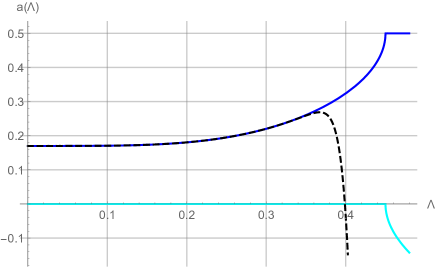
Figure 3: The black dashed line is the $a$ cycle derived with the recursion relation until ten instantons for $p=0.17$, the blue (cyan) line is the real (imaginary) part of the A-cycle derived with (44).

Here we demonstrate the numerical approach and compere it with the result of our recursion relation, then for large $q$ we give an analytic expression for $a$ and demonstrate that it is in agreement with the numerical method too.

To apply (44) we need the monodromy matrix, defined as in (42), where $f_{1}$ and $f_{2}$ are solutions to the Mathieu equation (38) with boundary conditions (39) and (40) respectively. As an example using Mathematica for $p=0.17$ and $\Lambda=0.2$ we find these solutions and their first order derivatives by solving the Mathieu equation numerically. The resulting monodromy matrix is

$$M=\left(\begin{array}[]{cc}0.423191\,+21.6727i&15.6243\\ 30.0101&0.423193\,-21.6727i\\ \end{array}\right)\,,$$ (47)

so that from (44) we get $a=0.180455$.

For $p=0.17$ and several values of $\Lambda$ we derived the A-cycle up to ten instantons using our recursion formula and compered it against the non perturbative numerical approach described above

$\Lambda$	$a$ by monodromy	$a$ by recursion
0.1	0.1706	0.1706
0.2	0.1804	0.1804
0.3	0.2202	0.2202
0.34	0.2508	0.2504
0.37	0.282	0.26819
0.4	0.3238	-0.0348
0.5	0.5 -0.1853 i	-3504.7

As it was expected these two approaches give close results provided the instanton counting parameter is small enough, in the table we kept five significant digits. To visualize this in Fig.3 for the fixed value $p=0.17$ we have plotted $a(\Lambda)$.

We can find analytically the large $\Lambda$ asymptotic behavior of $a$ from known results of (ODE/IM) correspondence Dorey:1998pt ; Bazhanov:1998wj . In this context two linearly independent solution $U_{0}(x,\Lambda)$ and $V_{0}(x,\Lambda)$ of Mathieu equation (38), uniquely specified by their behavior:

$${\rm for}\quad x\to\infty\quad U_{0}(x)\sim\sqrt{\frac{1}{u}}e^{-u}\quad{\rm where}\quad u=2\Lambda e^{\frac{x}{2}}$$

$${\rm for}\quad x\to-\infty\quad V_{0}(x)\sim\sqrt{\frac{1}{v}}e^{-v}\quad{\rm where}\quad v=2\Lambda e^{-\frac{x}{2}}$$

are considered. In Zamolodchikov:2000unpb ; Zamolodchikov:2000kt it was shown that one can define a Baxter’s $X(\theta)$ as the Wronskian of these two solutions (up to a $p$ independent factor it coincides with the spectral determinant of Mathieu operator)

$$X(\theta)=W[V_{0}(x,\theta),U_{0}(x,\theta)]$$ (48)

satisfying the functional relations

$$X(\theta+\frac{i\pi}{2})X(\theta-\frac{i\pi}{2})=1+X^{2}(\theta)\,,$$ (49)

$$T(\theta)X(\theta)=X(\theta+\frac{i\pi}{2})+X(\theta-\frac{i\pi}{2})\,.$$ (50)

Here $T(\theta)$ is an entire function and

$$\Lambda=\frac{\Gamma^{2}\left(\frac{1}{4}\right)}{16\sqrt{\pi}}e^{\theta}.$$ (51)

The specific choice of prefactor in (51) ensures a simple form of large $\theta$ asymptotic behavior for $X$:

$$X(\theta)\sim{\rm exp}\left(-\frac{\pi}{2}\,e^{\theta}\right)={\rm exp}\left(-\frac{8\pi^{3/2}\Lambda}{\Gamma^{2}\left(\frac{1}{4}\right)}\right)\,,$$ (52)

valid inside the strip $|{\rm Im}\theta|<\pi$. It was conjectured that the Floquet exponent $\mu$ of Mathieu equation is connected to $T(\theta)$ as

$$T=2\,\text{cos}\,(2\pi\mu)\,.$$ (53)

In Fioravanti:2019vxi ; Grassi:2019coc it was noticed that the Floquet exponent in the context of ${\cal N}=2$ SYM coincides with the A-cycle period $a$.

We can find the asymptomatic behavior for $a(\Lambda)$ straightforwardly by inserting (52) into (50) and taking into account (53), the result is

$$\text{cos}\,(2\pi a)\sim{\rm exp}\left(\frac{8\pi^{3/2}\Lambda}{\Gamma^{2}\left(\frac{1}{4}\right)}\right)\cos\left(\frac{8\pi^{3/2}\Lambda}{\Gamma^{2}\left(\frac{1}{4}\right)}\right)\,,$$ (54)

valid inside the strip $|\arg\Lambda|<\pi$.

Though $a$ is not a single valued function of $q$ nevertheless $\cos(2\pi a)$ behaves much better since $T$ is an entire function.

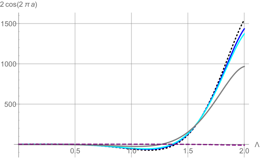
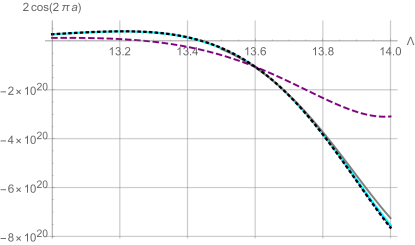
Figure 4: The graphics present the dependence of $2\cos(2\pi a)$ on $\Lambda$. The blue is for $p=0.1$, cyan for $p=0.2$, gray for $p=0.5$ and purple dashed for $p=2$. The black dotted line is the asymptotic curve given by (54). Notice that in the second picture $\Lambda$ reaches $14$ corresponding to $q=38416$.

These behavior is in agreement with the numerical results as presented in the table below, where $r$ is the ratio of the asymptotic and numerical values of $\cos 2\pi a$.

$\Lambda$	$\cos 2\pi a$ asymptotics	$\cos 2\pi a$ for $p=0.17$	$r$ for $p=0.17$	$r$ for $p=2$
$0.1$	$2.6471$	$0.9562$	$2.7683$	$1.3237$
$9$	$2.1446\times 10^{13}$	$2.1536\times 10^{13}$	$0.9958$	$1.4011$
$13$	$2.7087\times 10^{19}$	$2.6793\times 10^{19}$	$1.0109$	$2.2280$
$25$	$-1.2382\times 10^{37}$	$-1.2321\times 10^{37}$	$1.0049$	$1.3694$
$50$	$7.5854\times 10^{73}$	$7.5668\times 10^{73}$	$1.0025$	$1.1397$
$100$	$2.7545\times 10^{147}$	$2.7517\times 10^{147}$	$1.0011$	$1.0473$

Fig.4 demonstrates that $\cos(2\pi a)$ is quite regular in the interval $0\leq\Lambda\leq 14$, which includes the branch point of $a$ depicted in Fig.3. As one can see from (54) large $\Lambda$ asymptotic behavior is independent of $p$, nevertheless the smaller $p$ is, the faster the asymptotic region is reached.

4 $SU(2)$ SYM with hypermultiplets

In this section we are going to obtain a recursion relation for the A-cycle in the presence of several hypermultiplets. We will generalize the numerical approach using the differential equation for one fundamental hypermultiplet and demonstrate that the results are in agreement with the recursion relation.

From (10) we see

$$y(a)=P_{N_{f}}(a)-\frac{Q_{N_{f}}(a)}{y(a-1)}\,,\quad y(a-1)=P_{N_{f}}(a-1)-\frac{Q_{N_{f}}(a-1)}{y(a-2)}\,,\quad...\quad.$$ (55)

So that

$$y(a)=P_{N_{f}}(a)-\cfrac{Q_{N_{f}}(a)}{P_{N_{f}}(a-1)-\cfrac{Q_{N_{f}}(a-1)}{P_{N_{f}}(a-2)-\cfrac{Q_{N_{f}}(a-2)}{P_{N_{f}}(a-3)-...}}}\,.$$ (56)

Again from (10) we observe that

$$y(a)=\frac{Q_{N_{f}}(a+1)}{P_{N_{f}}(a+1)-y(a+1)}\,,\quad y(a+1)=\frac{Q_{N_{f}}(a+2)}{P_{N_{f}}(a+2)-y(a+2)}\,,\quad...\quad\,,$$ (57)

hence

$$y(a)=\cfrac{Q_{N_{f}}(a+1)}{P_{N_{f}}(a+1)-\cfrac{Q_{N_{f}}(a+2)}{P_{N_{f}}(a+2)-\cfrac{Q_{N_{f}}(a+3)}{P_{N_{f}}(a+3)-...}}}\,.$$ (58)

By taking the difference of (56) and (58) we will obtain our final recursion relation for the A-cycle (or alternatively $p^{2}$) for arbitrary number of flavors

$$P_{N_{f}}(a)-\cfrac{Q_{N_{f}}(a)}{P_{N_{f}}(a-1)-\cfrac{Q_{N_{f}}(a-1)}{P_{N_{f}}(a-2)-...}}-\cfrac{Q_{N_{f}}(a+1)}{P_{N_{f}}(a+1)-\cfrac{Q_{N_{f}}(a+2)}{P_{N_{f}}(a+2)-...}}=0\,,$$ (59)

where $P_{N_{f}}$ and $Q_{N_{f}}$ for arbitrary $N_{f}$ can be found in appendix A and like in the pure case the equality holds in the sense of power expansion in $q$. Below we do some explicit demonstration of these approach for four hypermultiplets.

The recursion (59) in one instanton order is

$$P_{4}(a)-\frac{Q_{4}(a)}{P_{4}(a-1)}-\frac{Q_{4}(a+1)}{P_{4}(a+1)}+O\left(q^{2}\right)=0\,,$$ (60)

where $P_{4}$ and $Q_{4}$ are given in (12) and (11) respectively. After inserting

$$a=a_{0}+a_{1}q+O\left(q^{2}\right)$$ (61)

one gets two equations by solving which determine $a_{0}$ and $a_{1}$ uniquely. Here is the result

$$a=p+\frac{-2\left(p^{4}+s_{4}\right)+p^{2}\left(s_{1}-2s_{2}\right)+s_{3}}{8p^{3}-2p}q+O\left(q^{2}\right)\,.$$ (62)

Results for two instantons can be found in appendix B. Alternatively we could considered

$$p^{2}=v_{0}+v_{1}+O\left(q^{2}\right)$$ (63)

leading to

$$p^{2}=a^{2}-\frac{-2\left(a^{4}+s_{4}\right)+a^{2}\left(s_{1}-2s_{2}\right)+s_{3}}{4a^{2}-1}q+O\left(q^{2}\right)\,.$$ (64)

To carry out computations for less number of flavors one should use coefficients (86)-(90).

Notice also that due to the AGT duality the four point conformal block in $2$d CFT is related to the instanton partition function with four hypermultiplets. This allows us to derive the heavy conformal block directly from recursions relation, as demonstrated in section 5.

4.1 Numerical method via the monodromy matrix when $N_{f}=1$

We shall generalize the method explored in subsection 3.3 for the cases with one hypermultiplet. Here instead of the Mathieu equation we have

$$\psi^{\prime\prime}(x)-\Lambda_{1}^{2}\left(e^{2x}+\frac{m}{\Lambda_{1}}e^{x}+e^{-x}\right)\psi(x)-p^{2}\psi(x)=0\,.$$ (65)

Once again, we have two solutions such that

$$\psi_{1}(0)=1\,,\quad\psi_{1}^{\prime}(0)=0\,,$$ (66)

$$\psi_{2}(0)=0\,,\quad\psi_{2}^{\prime}(0)=1\,.$$

Notice that their Wronskian is $W[\psi_{1}(x),\psi_{2}(x)]=1$. The monodromy matrix $M$ as in Mathieu case is defined by

$$\psi_{n}(x+2\pi i)=\sum_{k=1}^{2}\psi_{k}(x)M_{kn}\,.$$ (67)

Now it is easy to check that $W[\psi_{1}(2\pi i),\psi_{2}(2\pi i)]=\det M_{kn}=\mu_{1}\mu_{2}\,,$ where $\mu_{1}$ and $\mu_{2}$ are the eigenvalues of $M_{kn}$. So, taking into account that the Wronskian does not depend on $x$ we conclude that

$$\mu_{1}\mu_{2}=1\,.$$ (68)

It follows from (118) that (65) admits a quasiperiodic solution

$$\psi_{+}(x+2\pi i)=e^{2\pi ia}\psi_{+}(x)\,.$$ (69)

Hence one of the eigenvalues of $M$ is $e^{2\pi ia}$ but due to (68) the remaining eigenvalue must be $e^{-2\pi ia}$. Consequentially as in Mathieu case

$${\rm tr}M=2\cos(2\pi a)$$ (70)

and we can derive A-cycle numerically.

To summarize for fixed values of $\Lambda_{1}$, $p$ and $m$ we can numerically solve the differential equation (65) along the imaginary axis and find $\psi_{i}(2\pi i)$ and $\psi^{\prime}_{i}(2\pi i)$, $i=1,2$. As in the pure case we obtain the monodromy matrix (67) which with the help of (70) allows to derive $a$. Fig.5 demonstrates that numerical results derived with the instanton series (obtained through our recursion method) is in agreement with this numerical approach.

Notice that the above numerical approach based on differential equations can be successfully applied also for the cases with more hypermultiplets as well as in quiver theories and theories with higher rank gauge groups. The differential equations for these cases can be found in Poghossian:2016rzb ; Ashok:2016yxz .

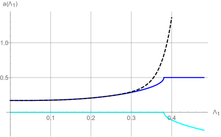
Figure 5: The black dashed line is the $a$ cycle derived with the recursion relation until five instanton for $p=0.17$, $m=0.7$, the blue line is the real part of the A-cycle and the cyan is its imaginary part derived with (70).

5 The recursion relation for the conformal block

In this section we will demonstrate how to use our recursion (59) to derive the conformal block. According to AGT conjecture Alday:2009aq the instanton partition function with $N_{f}=4$ antifundamental hypermultiplets is related to the generic $4$-point conformal block ${\cal B}$ as

$$Z_{inst}^{(4)}(a,m_{i},q)=x^{\Delta_{1}+\Delta_{2}-\Delta}(1-x)^{2(\lambda_{2}+\frac{Q}{2})(\lambda_{3}+\frac{Q}{2})}{\cal B}(\Delta,\Delta_{i},x),$$ (71)

where $\Delta_{i}$, $i=1,2,3,4$ are the dimensions of external (primary) fields (placed at the points $0$, $x$, $1$ and $\infty$ respectively) and $\Delta$ is the internal dimension parameterized as

$$\Delta_{i}=\frac{Q^{2}}{4}-\lambda_{i}^{2}\,,\hskip 28.45274pt\Delta=\frac{Q^{2}}{4}-\alpha^{2}\,.$$ (72)

$Q=b+1/b$ is related to the central charge of the Virasoro algebra through

$$c=1-6Q^{2}.$$ (73)

To define the heavy asymptotic limit let us introduce new parameters $\eta_{i}$ and $\eta$ by

$$\lambda_{i}=\frac{\eta_{i}}{b}\,,\qquad\alpha=\frac{\eta}{b}$$ (74)

and assume that in $b\to 0$ limit $\eta_{i}$ and $\eta$ are kept fixed. In this limit the conformal block ${\cal B}$ is conveniently represented as

$${\cal B}(\Delta,\Delta_{i},x)=e^{\frac{1}{b^{2}}f(\eta,\eta_{i},x)}\,$$ (75)

where the function $f(\eta,\eta_{i},x)$ has a finite limit at $b\to 0$.

AGT maps the instanton counting parameter $q$ to the cross ratio $x$ of insertion points in CFT block. The background charge parameter $b$ is related to the $\Omega$ background parameters by

$$b=\sqrt{\frac{\epsilon_{2}}{\epsilon_{1}}}\,,$$ (76)

the masses ot anti-fundamental hypermultiplet $m_{i}$ are related to CFT parameters as

$$\frac{m_{1}}{\sqrt{\epsilon_{1}\epsilon_{2}}} = \left(\lambda_{1}+\lambda_{2}+\frac{Q}{2}\right)\,,\,\,\frac{m_{2}}{\sqrt{\epsilon_{1}\epsilon_{2}}}=\left(\lambda_{2}-\lambda_{1}+\frac{Q}{2}\right)\,,\,\,$$ (77)

$$\frac{m_{3}}{\sqrt{\epsilon_{1}\epsilon_{2}}} = \left(\lambda_{3}+\lambda_{4}+\frac{Q}{2}\right)\,,\,\,\frac{m_{4}}{\sqrt{\epsilon_{1}\epsilon_{2}}}=\left(\lambda_{3}-\lambda_{4}+\frac{Q}{2}\right)\,$$ (78)

and finally the expectation value $a$ is related to the internal conformal dimension through

$$\frac{a}{\sqrt{\epsilon_{1}\epsilon_{2}}}=\alpha\,.$$ (79)

Thus from (79) and (76) in heavy limit we get

$$\frac{a}{\epsilon_{1}}=\eta$$ (80)

and similarly from (77) and (74)

$$\frac{m_{1}}{\epsilon_{1}} = \left(\eta_{1}+\eta_{2}+\frac{1}{2}\right)\,,\,\,\frac{m_{2}}{\epsilon_{1}}=\left(\eta_{2}-\eta_{1}+\frac{1}{2}\right)\,,\,\,$$ (81)

$$\frac{m_{3}}{\epsilon_{1}} = \left(\eta_{3}+\eta_{4}+\frac{1}{2}\right)\,,\,\,\frac{m_{4}}{\epsilon_{1}}=\left(\eta_{3}-\eta_{4}+\frac{1}{2}\right)\,.$$ (82)

From (4) and (71) we see that

$$\frac{F_{inst}}{\epsilon_{1}^{2}}=(\eta_{1}^{2}+\eta_{2}^{2}-\eta^{2}-\frac{1}{4})\log x-2\left(\eta_{2}+\frac{1}{2}\right)\left(\eta_{3}+\frac{1}{2}\right)\log(1-x)-f(\eta,\eta_{i},x)\,.$$ (83)

With the recursion relation (59) we can derive $u$ as a series in instanton counting parameter $q$ (see (64)) which can be inserted in the formula (5) allowing us to obtain $\frac{\partial F_{inst}}{\partial q}$. Integrating the result with respect to $q$ (integration constant is fixed from condition $f_{inst}\to 0$ when $q\to 0$) we can apply (83) and restore $f$ as a series in cross ratio $x$. The result is

$$f(\eta,\eta_{i},x)=(\eta_{1}^{2}+\eta_{2}^{2}-\eta^{2}-\frac{1}{4})\log x-\frac{\left(4\eta^{2}+4\eta_{2}^{2}-4\eta_{1}^{2}-1\right)\left(4\eta^{2}+4\eta_{3}^{2}-4\eta_{4}^{2}-1\right)}{8(4\eta^{2}-1)}x+...\,,$$ (84)

which is in agreement with known results in literature (for a recent paper see Litvinov:2013sxa ). The second order calculation can be inferred from (112).

Appendix A $P_{N_{f}}$ and $Q_{N_{f}}$ for less then four flavors

It is obvious from the expressions of $Q_{4}(z)$ and $P_{4}(z)$ above that they are invariant under the exchange of the masses. From here we can obtain the cases with less flavors by renormalizing the instanton coupling and sending some of the masses to infinity. To get the $N_{f}=0$ case from (11) and (12) we must simultaneously $m_{1}\to\mu,\dots,m_{4}\to\mu$, $q\to\frac{q}{\mu^{4}}$ and $\mu\to\infty$

$$P_{0}(z)=z^{2}-p^{2}\,,\quad Q_{0}(z)=q\,.$$ (85)

The procedure is similar for higher flavors:

• For $N_{f}=1$ $m_{i}\to\mu$, $i=1,2,3,$ $q\to\frac{q}{\mu^{3}}$ and then $\mu\to\infty$

  $$P_{1}(z)=z^{2}-p^{2}\,,$$ (86)

  $$Q_{1}(z)=q\left(m_{4}+z-1\right)\,.$$ (87)

• For $N_{f}=2$ $m_{i}\to\mu$, $i=1,2$ $q\to\frac{q}{\mu^{2}}$ and then $\mu\to\infty$

  $$P_{2}(z)=z^{2}-p^{2}+q\,,$$ (88)

  $$Q_{2}(z)=q\left(m_{3}+z-1\right)\left(m_{4}+z-1\right)\,.$$ (89)

• For $N_{f}=3$ $m_{1}\to\mu$ $q\to\frac{q}{\mu}$ and then $\mu\to\infty$

  $$P_{3}(z)=z^{2}-p^{2}+q(z-1)+\left(m_{2}+m_{3}+m_{4}\right)q\,,$$ (90)

  $$Q_{3}(z)=q\left(m_{2}+z-1\right)\left(m_{3}+z-1\right)\left(m_{4}+z-1\right)\,.$$ (91)

Appendix B A-cycle derivation for pure SYM

B.1 A-cycle derivation with the SW differential

We will derive the A-cycle from the formula (20) for pure SYM

$$a=\oint_{\mathcal{C}_{A}}\frac{dz}{2\pi i}z\partial_{z}\log y(z)\,,$$ (92)

where the contour $\mathcal{C}_{A}$ contains half of the poles in SW differential to be specified below. Let us write $y(z)$ as a series in $q$

$$y(z)=z^{2}-p^{2}+qy_{1}(z)+q^{2}y_{2}(z)+O(q)^{3}$$ (93)

after inserting this in (21) we will get

$$y_{1}(z)=\frac{1}{p^{2}-(z-1)^{2}};\quad y_{2}(z)=\frac{1}{\left(p^{2}-(z-2)^{2}\right)\left(p^{2}-(z-1)^{2}\right)^{2}}\,.$$ (94)

From here and (93) by direct computation we obtain

$$z\partial_{z}\log y(z)=\frac{2z^{2}}{z^{2}-p^{2}}+q\left(\frac{2z^{2}}{\left(z^{2}-p^{2}\right)^{2}\left((z-1)^{2}-p^{2}\right)}+\frac{2z(z-1)}{\left(z^{2}-p^{2}\right)\left((z-1)^{2}-p^{2}\right)^{2}}\right)+\qquad\qquad\qquad$$ (95)

$$+q^{2}\left(\frac{2z^{2}}{\left(p^{2}-(z-1)^{2}\right)^{2}\left(z^{2}-p^{2}\right)^{3}}+\frac{2z(1-z)}{\left(p^{2}-(z-1)^{2}\right)^{3}\left(z^{2}-p^{2}\right)^{2}}-\frac{2z^{2}}{\left(p^{2}-(z-1)^{2}\right)^{2}\left(p^{2}-(z-2)^{2}\right)\left(z^{2}-p^{2}\right)^{2}}+\right.$$

$$\qquad+\left.\frac{4(z-1)z}{\left(p^{2}-(z-1)^{2}\right)^{3}\left(p^{2}-(z-2)^{2}\right)\left(z^{2}-p^{2}\right)}+\frac{2(z-2)z}{\left(p^{2}-(z-1)^{2}\right)^{2}\left(p^{2}-(z-2)^{2}\right)^{2}\left(z^{2}-p^{2}\right)}\right)+O\left(q^{3}\right)\,.$$

To derive the A-cycle we need to insert the last result in (92) and perform integration. From the above expression we observe that the poles of it are located at:

$$q^{0}:\quad\pm p$$

$$q^{1}:\quad\pm p,\quad\pm p+1$$

$$q^{2}:\quad\pm p,\quad\pm p+1,\quad\pm p+2$$

The contour $\mathcal{C}_{A}$ encloses all the poles where $p$ appears with plus sign (the alternative choice with minus signs would give $-a$ instead). The final result is (37).

B.2 $A$ cycle period for pure SYM via instanton counting

We can derive $u$ by using (1) together with (2.1). The result is

$$Z_{inst}=1+\frac{2q}{\epsilon_{1}\epsilon_{2}\left(-2a+\epsilon_{1}+\epsilon_{2}\right)\left(2a+\epsilon_{1}+\epsilon_{2}\right)}+$$ (96)

$$+\frac{q^{2}\left(-8a^{2}+8\epsilon_{1}^{2}+8\epsilon_{2}^{2}+17\epsilon_{1}\epsilon_{2}\right)}{\epsilon_{1}^{2}\epsilon_{2}^{2}\left(-2a+\epsilon_{1}+\epsilon_{2}\right)\left(2a+\epsilon_{1}+\epsilon_{2}\right)\left(-2a+2\epsilon_{1}+\epsilon_{2}\right)\left(2\left(a+\epsilon_{1}\right)+\epsilon_{2}\right)\left(-2a+\epsilon_{1}+2\epsilon_{2}\right)\left(2\left(a+\epsilon_{2}\right)+\epsilon_{1}\right)}+O\left(q^{3}\right)\,.$$

After inserting this in (4) we will obtain

$$F_{inst}(a,\epsilon,q)=\frac{2q}{4a^{2}-\epsilon^{2}}+\frac{q^{2}\left(20a^{2}+7\epsilon^{2}\right)}{4\left(a^{2}-\epsilon^{2}\right)\left(4a^{2}-\epsilon^{2}\right)^{3}}+O\left(q^{3}\right)\,.$$ (97)

Thus from (5) we will get

$$u=2a^{2}+\frac{4q}{4a^{2}-\epsilon^{2}}+\frac{q^{2}\left(20a^{2}+7\epsilon^{2}\right)}{\left(a^{2}-\epsilon^{2}\right)\left(4a^{2}-\epsilon^{2}\right)^{3}}+O\left(q^{3}\right)\,.$$ (98)

This coincides with (34) after setting $\epsilon=1$. By inverting this series we will arrive at (37).

Appendix C Two instanton expressions for the $A$ cycle period with $N_{f}=4,3,2,1$ flavors

In this section we perform two instanton computations using our recursion relation (59). In two instanton approximation we have

$$0=P_{N_{f}}(a)-\cfrac{Q_{N_{f}}(a)}{P_{N_{f}}(a-1)-\cfrac{Q_{N_{f}}(a-1)}{P_{N_{f}}(a-2)}}-\cfrac{Q_{N_{f}}(a+1)}{P_{N_{f}}(a+1)-\cfrac{Q_{N_{f}}(a+2)}{P_{N_{f}}(a+2)}}+O\left(q^{3}\right)\,.$$ (99)

Using (11), (12) (or (86)-(90) for the cases with less number of flavors) and inserting the expansion

$$a=a_{0}+a_{1}q+a_{2}q^{2}+O\left(q^{3}\right)$$ (100)

into (99) we’ll find equations, uniquely specifying the coefficients $a_{0}$, $a_{1}$ and $a_{2}$. Here are the results:
$\bullet$ For $N_{f}=1$

$$a=p+\frac{\left(1-2m_{4}\right)q}{8p^{3}-2p}+\frac{q^{2}\left(-2\left(m_{4}-1\right)m_{4}\left(60p^{4}-35p^{2}+2\right)+24p^{6}-42p^{4}+19p^{2}-1\right)}{8p^{3}\left(p^{2}-1\right)\left(4p^{2}-1\right)^{3}}+O\left(q^{3}\right)\,,$$ (101)

$$p^{2}=a^{2}+\frac{\left(1-2m_{4}\right)q}{1-4a^{2}}+\frac{q^{2}\left(-12a^{4}+\left(20a^{2}+7\right)\left(m_{4}-1\right)m_{4}+11a^{2}+1\right)}{2\left(a^{2}-1\right)\left(4a^{2}-1\right)^{3}}+O\left(q^{3}\right)\,,\qquad\qquad$$ (102)

$\bullet$ For $N_{f}=2$

$$a=p+\frac{s_{1}-2\left(p^{2}+s_{2}\right)}{8p^{3}-2p}q+\frac{A_{2}}{8p^{3}\left(p^{2}-1\right)\left(4p^{2}-1\right)^{3}}q^{2}+O\left(q^{3}\right)\,,$$ (103)

$$p^{2}=a^{2}+\frac{2\left(a^{2}+s_{2}\right)-s_{1}}{4a^{2}-1}q+\frac{p_{2}}{2\left(a^{2}-1\right)\left(4a^{2}-1\right)^{3}}q^{2}+O\left(q^{3}\right)\,,$$ (104)

where

$$A_{2}=2s_{1}\left((p-1)(p+1)\left(12p^{2}+1\right)p^{2}+\left(60p^{4}-35p^{2}+2\right)s_{2}\right)-\qquad\quad$$ (105)

$$-2\left(p^{2}+s_{2}\right)\left((p-1)(p+1)\left(12p^{2}+1\right)p^{2}+\left(60p^{4}-35p^{2}+2\right)s_{2}\right)+$$

$$+\left(24p^{6}-42p^{4}+19p^{2}-1\right)s_{1}^{2}\,,$$

$$p_{2}=\left(20a^{2}+7\right)s_{2}^{2}+\left(a^{2}-1\right)\left(a^{2}\left(4a^{2}-5\right)-\left(12a^{2}+1\right)\left(s_{1}-1\right)s_{1}\right)+$$ (106)

$$+s_{2}\left(24a^{4}-\left(20a^{2}+7\right)s_{1}-2a^{2}+5\right)\,,$$

where $s_{1}$ and $s_{2}$ are elementary symmetric polynomials in $m_{3}$ and $m_{4}$ (i.e. $s_{1}=m_{3}+m_{4}$ and $s_{2}=m_{3}m_{4}$).
$\bullet$ For $N_{f}=3$

$$a=p+\frac{-2p^{2}s_{1}+p^{2}+s_{2}-2s_{3}}{8p^{3}-2p}q+\frac{A_{2}}{8p^{3}\left(p^{2}-1\right)\left(4p^{2}-1\right)^{3}}q^{2}+O\left(q^{3}\right)\,,$$ (107)

$$p^{2}=a^{2}+\frac{-2a^{2}s_{1}+a^{2}+s_{2}-2s_{3}}{1-4a^{2}}q+\frac{p_{2}}{2\left(a^{2}-1\right)\left(4a^{2}-1\right)^{3}}q^{2}+O\left(q^{3}\right)\,,$$ (108)

where

$$A_{2}=2p^{2}s_{1}\left((p-1)(p+1)\left(12p^{2}+1\right)\left(p^{2}+s_{2}\right)+\left(-72p^{4}+46p^{2}-1\right)s_{3}\right)-\qquad\qquad\qquad$$

$$-2\left(60p^{4}-35p^{2}+2\right)s_{3}^{2}+2\left(60p^{4}-35p^{2}+2\right)s_{3}\left(p^{2}+s_{2}\right)+\left(-24p^{8}+22p^{6}+2p^{4}\right)s_{1}^{2}-$$

$$-(p-1)(p+1)\left(p^{2}+s_{2}\right)\left(8p^{6}+2p^{4}+p^{2}+\left(-24p^{4}+18p^{2}-1\right)s_{2}\right)\,,\qquad\qquad$$ (109)

$$p_{2}=\left(20a^{2}+7\right)s_{3}^{2}+\left(a^{2}-1\right)a^{2}\left(4a^{4}+\left(4a^{2}-5\right)\left(s_{1}-1\right)s_{1}-a^{2}-1\right)+\quad$$

$$+\left(-12a^{4}+11a^{2}+1\right)s_{2}^{2}-\left(a^{2}-1\right)s_{2}\left(8a^{4}-\left(12a^{2}+1\right)s_{1}+2a^{2}+1\right)+$$ (110)

$$+s_{3}\left(-36a^{4}-\left(20a^{2}+7\right)s_{2}+13a^{2}+\left(24a^{4}-2a^{2}+5\right)s_{1}-4\right)\,.\,\,$$

In this case $s_{1}$, $s_{2}$ and $s_{3}$ are the elementary symmetric polynomials in $m_{1}$, $m_{2}$ and $m_{3}$ (i.e. $s_{1}=m_{1}+m_{2}+m_{3}$, $s_{2}=m_{1}m_{2}+m_{1}m_{3}+m_{2}m_{3}$, $s_{3}=m_{1}m_{2}m_{3}$).
$\bullet$ For $N_{f}=4$

$$a=p+\frac{-2\left(p^{4}+s_{4}\right)+p^{2}\left(s_{1}-2s_{2}\right)+s_{3}}{8p^{3}-2p}q+\frac{A_{2}}{8p^{3}\left(p^{2}-1\right)\left(4p^{2}-1\right)^{3}}q^{2}+O\left(q^{3}\right)\,,$$ (111)

$$p^{2}=a^{2}-\frac{-2\left(a^{4}+s_{4}\right)+a^{2}\left(s_{1}-2s_{2}\right)+s_{3}}{4a^{2}-1}q+\frac{p_{2}}{2\left(a^{2}-1\right)\left(4a^{2}-1\right)^{3}}q^{2}+O\left(q^{3}\right)\,,$$ (112)

where

$$A_{2}=2p^{2}s_{1}\left(\left(p^{2}-1\right)p^{2}\left(28p^{4}+\left(12p^{2}+1\right)s_{2}+2\left(4p^{2}-5\right)s_{3}-7p^{2}+1\right)+\left(60p^{4}-35p^{2}+2\right)s_{4}\right)-$$

$$-2\left(60p^{4}-35p^{2}+2\right)s_{4}^{2}+(p-1)(p+1)\left(-2p^{4}\left(p^{2}+s_{2}\right)\left(28p^{4}+\left(12p^{2}+1\right)s_{2}-7p^{2}+1\right)+\right.$$

$$\left.+2p^{2}s_{3}\left(28p^{4}+\left(12p^{2}+1\right)s_{2}-7p^{2}+1\right)+\left(24p^{4}-18p^{2}+1\right)s_{3}^{2}\right)-2s_{4}\left(\left(-60p^{4}+35p^{2}-2\right)s_{3}+\right.$$

$$\left.+p^{2}\left(88p^{6}-70p^{4}+10p^{2}+\left(72p^{4}-46p^{2}+1\right)s_{2}-1\right)\right)+\left(-8p^{10}+6p^{8}+p^{6}+p^{4}\right)s_{1}^{2}$$

$$p_{2}=\left(20a^{2}+7\right)s_{4}^{2}+\left(a^{2}-1\right)\left(-\left(12a^{2}+1\right)s_{3}^{2}+a^{2}\left(a^{2}+s_{2}\right)\left(52a^{4}+\left(4a^{2}-5\right)s_{2}-21a^{2}+1\right)+\right.$$

$$\left.+s_{3}\left(-20a^{4}+\left(12a^{2}+1\right)s_{2}+13a^{2}-1\right)\right)+\left(4a^{8}-5a^{6}+a^{2}\right)s_{1}^{2}+s_{1}\left(\left(-36a^{4}+13a^{2}-4\right)s_{4}-\right.$$

$$-\left.\left(a^{2}-1\right)\left(36a^{6}-17a^{4}+\left(4a^{2}-5\right)a^{2}s_{2}+a^{2}+\left(8a^{4}+2a^{2}+1\right)s_{3}\right)\right)+$$

$$+s_{4}\left(72a^{6}-66a^{4}-\left(20a^{2}+7\right)s_{3}+22a^{2}+\left(24a^{4}-2a^{2}+5\right)s_{2}-1\right)\,\,$$

Appendix D From the difference equation to the differential equation

In this section we will derive differential equations from the difference equation (8) with the help of inverse Fourier transform:

$$f(x)=\sum_{z\in\mathbb{Z}+a}e^{x(z+1)}Y(z)\,.$$ (113)

D.1 From the difference equation to Mathieu equation

According to (8), the difference equation for pure SYM (85) is

$$Y(z+1)+qY(z-1)-\left((z+1)^{2}-p^{2}\right)Y(z)=0\,.$$ (114)

By means of inverse Fourier transform (113) we can derive the following second order differential equation

$$f^{\prime\prime}(x)-\left(qe^{x}+e^{-x}+p^{2}\right)f(x)=0\,.$$ (115)

Shifting $x$ by $\sqrt{q}$ one immediately arrives at the Mathieu equation (38), where $q=\Lambda^{4}$.

Appendix E The differential equation for $N_{f}=1$

The cases with flavors are similar to the pure one. When $N_{f}=1$ we have (86), so that (8) becomes

$$Y(z+1)+q(m_{4}+z)Y(z-1)-((z+1)^{2}-p^{2})Y(z)=0\,.$$ (116)

From this and (113) we obtain

$$f^{\prime\prime}(x)-qe^{x}f^{\prime}(x)-\left(qm_{4}e^{x}+e^{-x}+p^{2}\right)f(x)=0\,.$$ (117)

By taking

$$f(x)=e^{\frac{qe^{x}}{2}}\psi(x)\,,$$ (118)

it is straightforward to see that

$$\psi^{\prime\prime}(x)-\left(\frac{1}{4}q^{2}e^{2x}+\left(m_{4}-\frac{1}{2}\right)qe^{x}+e^{-x}+p^{2}\right)\psi(x)=0\,.$$ (119)

Shifting $x\to x-\frac{2}{3}{\rm ln}(q/2)$ one gets

$$\psi^{\prime\prime}(x)-\left(\frac{q}{2}\right)^{2/3}\left(e^{2x}+2\left(m_{4}-\frac{1}{2}\right)\left(\frac{q}{2}\right)^{-1/3}e^{x}+e^{-x}\right)\psi(x)-p^{2}\psi(x)=0\,.$$ (120)

Using the notations

$$m\equiv 2\left(m_{4}-\frac{1}{2}\right)\,,\quad\Lambda_{1}\equiv\left(\frac{q}{2}\right)^{1/3}\,,$$ (121)

we will obtain (65).

References

• (1) A. Lossev, N. Nekrasov, and S. L. Shatashvili, Testing Seiberg-Witten solution, in Strings, branes and dualities. Proceedings, NATO Advanced Study Institute, Cargese, France, May 26-June 14, 1997, 1997. [hep-th/9801061].
• (2) N. A. Nekrasov, Seiberg-Witten prepotential from instanton counting, Adv. Theor. Math. Phys. 7 (2003), no. 5 831–864, [hep-th/0206161].
• (3) R. Flume and R. Poghossian, An Algorithm for the microscopic evaluation of the coefficients of the Seiberg-Witten prepotential, Int. J. Mod. Phys. A18 (2003) 2541, [hep-th/0208176].
• (4) N. Nekrasov and A. Okounkov, Seiberg-Witten theory and random partitions, Prog. Math. 244 (2006) 525–596, [hep-th/0306238].
• (5) U. Bruzzo, F. Fucito, J. F. Morales, and A. Tanzini, Multiinstanton calculus and equivariant cohomology, JHEP 05 (2003) 054, [hep-th/0211108].
• (6) N. A. Nekrasov and S. L. Shatashvili, Quantization of Integrable Systems and Four Dimensional Gauge Theories, in Proceedings, 16th International Congress on Mathematical Physics (ICMP09), 2009. [arXiv:0908.4052].
• (7) L. F. Alday, D. Gaiotto, and Y. Tachikawa, Liouville Correlation Functions from Four-dimensional Gauge Theories, Lett. Math. Phys. 91 (2010) 167–197, [arXiv:0906.3219].
• (8) N. Seiberg, Notes on quantum Liouville theory and quantum gravity, Prog. Theor. Phys. Suppl. 102 (1990) 319–349.
• (9) A. B. Zamolodchikov and A. B. Zamolodchikov, Structure constants and conformal bootstrap in Liouville field theory, Nucl. Phys. B477 (1996) 577–605, [hep-th/9506136].
• (10) A. B. Zamolodchikov, Conformal symmetry in two-dimensions: an explicit recurrence formula for the conformal partial wave amplitude, Commun. Math. Phys. 96 (1984) 419–422.
• (11) A. B. Zamolodchikov, Conformal symmetry in two-dimensional space: recursion representation of conformal block, Theor. Math. Phys. 73 (1987) 1088–1093.
• (12) R. Poghossian, Recursion relations in CFT and N=2 SYM theory, JHEP 12 (2009) 038, [arXiv:0909.3412].
• (13) R. Poghossian, Recurrence relations for the ${\mathcal{W}}_{3}$ conformal blocks and $\mathcal{N}=2$ SYM partition functions, JHEP 11 (2017) 053, [arXiv:1705.00629]. [Erratum: JHEP 01, 088 (2018)].
• (14) L. Hadasz, Z. Jaskolski, and P. Suchanek, Recursion representation of the Neveu-Schwarz superconformal block, JHEP 03 (2007) 032, [hep-th/0611266].
• (15) L. Hadasz, Z. Jaskolski, and P. Suchanek, Elliptic recurrence representation of the N=1 superconformal blocks in the Ramond sector, JHEP 11 (2008) 060, [arXiv:0810.1203].
• (16) S. Alekseev, A. Gorsky, and M. Litvinov, Toward the Pole, JHEP 03 (2020) 157, [arXiv:1911.01334].
• (17) M. Beccaria, On the large $\Omega$-deformations in the Nekrasov-Shatashvili limit of $\mathcal{N}=2^{*}$ SYM, JHEP 07 (2016) 055, [arXiv:1605.00077].
• (18) A. Gorsky, A. Milekhin, and N. Sopenko, Bands and gaps in Nekrasov partition function, JHEP 01 (2018) 133, [arXiv:1712.02936].
• (19) R. Poghossian, Deforming SW curve, JHEP 04 (2011) 033, [arXiv:1006.4822].
• (20) N. Seiberg and E. Witten, Electric - magnetic duality, monopole condensation, and confinement in N=2 supersymmetric Yang-Mills theory, Nucl. Phys. B426 (1994) 19–52, [hep-th/9407087]. [Erratum: Nucl. Phys.B430,485(1994)].
• (21) N. Seiberg and E. Witten, Monopoles, duality and chiral symmetry breaking in N=2 supersymmetric QCD, Nucl. Phys. B431 (1994) 484–550, [hep-th/9408099].
• (22) M. x. Huang, A. K. Kashani-Poor and A. Klemm, Annales Henri Poincare 14, 425-497 (2013) doi:10.1007/s00023-012-0192-x [arXiv:1109.5728].
• (23) M. x. Huang, A. Klemm, J. Reuter and M. Schiereck, JHEP 02 (2015), 031 doi:10.1007/JHEP02(2015)031 [arXiv:1401.4723].
• (24) F. Fucito, J. F. Morales, D. R. Pacifici, and R. Poghossian, Gauge theories on $\Omega$-backgrounds from non commutative Seiberg-Witten curves, JHEP 05 (2011) 098, [arXiv:1103.4495].
• (25) A. Mironov and A. Morozov, Nekrasov Functions and Exact Bohr-Zommerfeld Integrals, JHEP 04 (2010) 040, [arXiv:0910.5670].
• (26) A. Mironov and A. Morozov, Nekrasov Functions from Exact BS Periods: The Case of SU(N), J. Phys. A43 (2010) 195401, [arXiv:0911.2396].
• (27) K. Maruyoshi and M. Taki, Deformed Prepotential, Quantum Integrable System and Liouville Field Theory, Nucl. Phys. B 841 (2010) 388–425, [arXiv:1006.4505].
• (28) G. Wolf, Mathieu Functions and Hill’s EquationNIST Digital Library of Mathematical Functions.” https://dlmf.nist.gov/28.
• (29) A. Zamolodchikov, Generalized Mathieu equation and Liouville TBA, 2000, in Quantum Field Theories in Two Dimensions, vol. 2, World Scientific, 2012.
• (30) D. Fioravanti, H. Poghosyan, and R. Poghossian, $T$, $Q$ and periods in $SU(3)$ ${\cal N}=2$ SYM, JHEP 03 (2020) 049, [arXiv:1909.11100].
• (31) N. Nekrasov, BPS/CFT correspondence: non-perturbative Dyson-Schwinger equations and qq-characters, [arXiv:1512.05388].
• (32) G. Poghosyan and R. Poghossian, VEV of Baxter’s Q-operator in N=2 gauge theory and the BPZ differential equation, JHEP 11 (2016) 058, [arXiv:1602.02772].
• (33) G. Poghosyan, VEV of $Q$-operator in $U(1)$ linear quiver 5d gauge theories, [arXiv:1801.04303].
• (34) N. Nekrasov, V. Pestun and S. Shatashvili, Commun. Math. Phys. 357, no.2, 519-567 (2018) doi:10.1007/s00220-017-3071-y [arXiv:1312.6689].
• (35) P. Dorey and R. Tateo, J. Phys. A 32, L419-L425 (1999) doi:10.1088/0305-4470/32/38/102, [arXiv:9812211].
• (36) V. V. Bazhanov, S. L. Lukyanov and A. B. Zamolodchikov, J. Statist. Phys. 102, 567-576 (2001) doi:10.1023/A:1004838616921 [arXiv:9812247].
• (37) P. Dorey, C. Dunning and R. Tateo, J. Phys. A 40, R205 (2007) doi:10.1088/1751-8113/40/32/R01, [arXiv:0703066].
• (38) A. B. Zamolodchikov, On the thermodynamic Bethe ansatz equation in sinh-Gordon model, J. Phys. A 39 (2006) 12863–12887, [hep-th/0005181].
• (39) M. Matone, Instantons and recursion relations in N=2 SUSY gauge theory, Phys. Lett. B357 (1995) 342–348, [hep-th/9506102].
• (40) R. Flume, F. Fucito, J. F. Morales, and R. Poghossian, Matone’s relation in the presence of gravitational couplings, JHEP 04 (2004) 008, [hep-th/0403057].
• (41) D. Fioravanti and D. Gregori, Integrability and cycles of deformed ${\cal N}=2$ gauge theory, [arXiv:1908.08030].
• (42) A. Grassi, J. Gu and M. Mariño, JHEP 07 (2020), 106 doi:10.1007/JHEP07(2020)106 [arXiv:1908.07065].
• (43) R. Poghossian, Deformed SW curve and the null vector decoupling equation in Toda field theory, [arXiv:1601.05096].
• (44) S. K. Ashok, D. P. Jatkar, R. R. John, M. Raman, and J. Troost, Exact WKB analysis of $\mathcal{N}$ = 2 gauge theories, JHEP 07 (2016) 115, [arXiv:1604.05520].
• (45) A. Litvinov, S. Lukyanov, N. Nekrasov, and A. Zamolodchikov, Classical Conformal Blocks and Painleve VI, JHEP 07 (2014) 144, [arXiv:1309.4700].