ONLINE NON-CONVEX OPTIMIZATION WITH IMPERFECT FEEDBACK

Abstract.

We consider the problem of online learning with non-convex losses. In terms of feedback, we assume that the learner observes – or otherwise constructs – an inexact model for the loss function encountered at each stage, and we propose a mixed-strategy learning policy based on dual averaging. In this general context, we derive a series of tight regret minimization guarantees, both for the learner’s static (external) regret, as well as the regret incurred against the best dynamic policy in hindsight. Subsequently, we apply this general template to the case where the learner only has access to the actual loss incurred at each stage of the process. This is achieved by means of a kernel-based estimator which generates an inexact model for each round’s loss function using only the learner’s realized losses as input.

1. Introduction

In this paper, we consider the following online learning framework:

1. At each stage $t=1,2,\dotsc$ of a repeated decision process, the learner selects an action $x_{t}$ from a compact convex subset $\mathcal{K}$ of a Euclidean space $\mathbb{R}^{n}$.

2. The agent’s choice of action triggers a loss $\ell_{t}(x_{t})$ based on an a priori unknown loss function $\ell_{t}\colon\mathcal{K}\to\mathbb{R}$; subsequently, the process repeats.

If the loss functions $\ell_{t}$ encountered by the agent are convex, the above framework is the standard online convex optimization setting of Zinkevich [58] – for a survey, see [45, 16, 29] and references therein. In this case, simple first-order methods like online gradient descent (OGD) allow the learner to achieve $\operatorname{\mathcal{O}}(T^{1/2})$ regret after $T$ rounds [58], a bound which is well-known to be min-max optimal in this setting [1, 45]. At the same time, it is also possible to achieve tight regret minimization guarantees against dynamic comparators – such as the regret incurred against the best dynamic policy in hindsight, cf. [23, 21, 11, 30, 33] and references therein.

On the other hand, when the problem’s loss functions are not convex, the situation is considerably more difficult. When the losses are generated from a stationary stochastic distribution, the problem can be seen as a version of a continuous-armed bandit in the spirit of Agrawal [3]; in this case, there exist efficient algorithms guaranteeing logarithmic regret by discretizing the problem’s search domain and using a UCB-type policy [18, 37, 48]. Otherwise, in an adversarial context, an informed adversary can impose linear regret to any deterministic algorithm employed by the learner [45, 31, 50]; as a result, UCB-type approaches are no longer suitable.

In view of this impossibility result, two distinct threads of literature have emerged for online non-convex optimization. One possibility is to examine less demanding measures of regret – like the learner’s local regret [31] – and focus on first-order methods that minimize it efficiently [31, 28]. Another possibility is to consider randomized algorithms, in which case achieving no regret is possible: Krichene et al. [38] showed that adapting the well-known Hedge (or multiplicative / exponential weights) algorithm to a continuum allows the learner to achieve $\operatorname{\mathcal{O}}(T^{1/2})$ regret, as in the convex case. This result is echoed in more recent works by Agarwal et al. [2] and Suggala & Netrapalli [50] who analyzed the “follow the perturbed leader” (FTPL) algorithm of Kalai & Vempala [34] with exponentially distributed perturbations and an offline optimization oracle (exact or approximate); again, the regret achieved by “follow the perturbed leader” (FTPL) in this setting is $\operatorname{\mathcal{O}}(T^{1/2})$, i.e., order-equivalent to that of Hedge in a continuum.

Our contributions and related work.

A crucial assumption in the above works on randomized algorithms is that, after selecting an action, the learner receives perfect information on the loss function encountered – i.e., an exact model thereof. This is an important limitation for the applicability of these methods, which led to the following question by Krichene et al. [38, p. 8]:

One question is whether one can generalize the Hedge algorithm to a bandit setting, so that sublinear regret can be achieved without the need to explicitly maintain a cover.

To address this open question, we begin by considering a general framework for randomized action selection with imperfect feedback – i.e., with an inexact model of the loss functions encountered at each stage. Our contributions in this regard are as follows:

1. We present a flexible algorithmic template for online non-convex learning based on dual averaging with imperfect feedback [42].

2. We provide tight regret minimization rates – both static and dynamic – under a wide range of different assumptions for the loss models available to the optimizer.

3. We show how this framework can be extended to learning with bandit feedback, i.e., when the learner only observes their realized loss and must construct a loss model from scratch.

Viewed abstractly, the dual averaging (DA) algorithm is an “umbrella” scheme that contains Hedge as a special case for problems with a simplex-like domain. In the context of online convex optimization, the method is closely related to the well-known “follow the regularized leader” (FTRL) algorithm of Shalev-Shwartz & Singer [46], the FTPL method of Kalai & Vempala [34], “lazy” mirror descent (MD) [45, 16, 15], etc. For an appetizer to the vast literature surrounding these methods, we refer the reader to [46, 42, 45, 55, 16, 14, 57] and references therein.

	Convex Losses		Non-Convex Losses
Feedback	Static regret	Dynamic regret	Static regret	Dynamic regret
Exact	$\operatorname{\mathcal{O}}\big{(}T^{1/2}\big{)}$   [58]	$\operatorname{\mathcal{O}}\big{(}T^{2/3}V_{T}^{1/3}\big{)}$   [11]	$\operatorname{\mathcal{O}}\big{(}T^{1/2}\big{)}$   [38, 50]	$\boldsymbol{\operatorname{\mathcal{O}}\big{(}T^{2/3}V_{T}^{1/3}\big{)}}$
Unbiased	$\operatorname{\mathcal{O}}\big{(}T^{1/2}\big{)}$   [58]	$\operatorname{\mathcal{O}}\big{(}T^{2/3}V_{T}^{1/3}\big{)}$   [11]	$\boldsymbol{\operatorname{\mathcal{O}}\big{(}T^{1/2}\big{)}}$	$\boldsymbol{\operatorname{\mathcal{O}}\big{(}T^{2/3}V_{T}^{1/3}\big{)}}$
Bandit	$\operatorname{\mathcal{O}}\big{(}T^{1/2}\big{)}$   [17, 19]	$\operatorname{\mathcal{O}}\big{(}T^{4/5}V_{T}^{1/5}\big{)}$   [11]	$\boldsymbol{\operatorname{\mathcal{O}}\big{(}T^{\frac{n+2}{n+3}}\big{)}}$	$\boldsymbol{\operatorname{\mathcal{O}}\big{(}T^{\frac{n+3}{n+4}}V_{T}^{\frac{1^{\vphantom{1}}}{n+4}}\big{)}}$

Table 1. Overview of related work. In regards to feedback, an “exact” model means that the learner acquires perfect knowledge of the encountered loss functions; “unbiased” refers to an inexact model that is only accurate on average; finally, “bandit” means that the learner records their incurred loss and has no other information. We only report here the best known bounds in the literature; all bounds derived in this paper are typeset in bold.

In the non-convex setting, our regret minimization guarantees can be summarized as follows (see also Table 1 above): if the learner has access to inexact loss models that are unbiased and finite in mean square, the DA algorithm achieves in expectation a static regret bound of $\operatorname{\mathcal{O}}(T^{1/2})$. Moreover, in terms of the learner’s dynamic regret, the algorithm enjoys a bound of $\operatorname{\mathcal{O}}(T^{2/3}V_{T}^{1/3})$ where $V_{T}\coloneqq\sum\nolimits_{t=1}^{T}\lVert\ell_{t+1}-\ell_{t}\rVert_{\infty}$ denotes the variation of the loss functions encountered over the horizon of play (cf. Section 4 for the details). Importantly, both bounds are order-optimal, even in the context of online convex optimization, cf. [20, 11, 1].

With these general guarantees in hand, we tackle the bandit setting using a “kernel smoothing” technique in the spirit of Bubeck et al. [19]. This leads to a new algorithm, which we call bandit dual averaging (BDA), and which can be seen as a version of the DA method with biased loss models. The bias of the loss model can be controlled by tuning the “radius” of the smoothing kernel; however, this comes at the cost of increasing the model’s variance – an incarnation of the well-known “bias-variance” trade-off. By resolving this trade-off, we are finally able to answer the question of Krichene et al. [38] in the positive: bandit dual averaging (BDA) enjoys an $\operatorname{\mathcal{O}}(T^{\frac{n+2}{n+3}})$ static regret bound and an $\operatorname{\mathcal{O}}(T^{\frac{n+3}{n+4}}V_{T}^{1/(n+4)})$ dynamic regret bound, without requiring an explicit discretization of the problem’s search space.

This should be contrasted with the case of online convex learning, where it is possible to achieve $\operatorname{\mathcal{O}}(T^{3/4})$ regret through the use of simultaneous perturbation stochastic approximation (SPSA) techniques [25], or even $\operatorname{\mathcal{O}}(T^{1/2})$ by means of kernel-based methods [17, 19]. This represents a drastic drop from $\operatorname{\mathcal{O}}(T^{1/2})$, but this cannot be avoided: the worst-case bound for stochastic non-convex optimization is $\Omega(T^{(n+1)/(n+2)})$ [36, 37], so our static regret bound is nearly optimal in this regard (i.e., up to $\operatorname{\mathcal{O}}(T^{-1/(n+2)(n+3)})$, a term which is insignificant for horizons $T\leq 10^{12}$). Correspondingly, in the case of dynamic regret minimization, the best known upper bound is $\operatorname{\mathcal{O}}(T^{4/5}V_{T}^{1/5})$ for online convex problems [11, 24]. We are likewise not aware of any comparable dynamic regret bounds for online non-convex problems; to the best our knowledge, our paper is the first to derive dynamic regret guarantees for online non-convex learning with bandit feedback.

We should stress here that, as is often the case for methods based on lifting, much of the computational cost is hidden in the sampling step. This is also the case for the proposed DA method which, like [38], implicitly assumes access to a sampling oracle. Estimating (and minimizing) the per-iteration cost of sampling is an important research direction, but one that lies beyond the scope of the current paper, so we do not address it here.

2. Setup and preliminaries

2.1. The model

Throughout the sequel, our only blanket assumption will be as follows:

Assumption 1.

The stream of loss functions encountered is uniformly bounded Lipschitz, i.e., there exist constants $R,L>0$ such that:

1. $\lvert\ell_{t}(x)\rvert\leq R$ for all $x\in\mathcal{K}$; more succinctly, $\lVert\ell_{t}\rVert_{\infty}\leq R$.

2. $\lvert\ell_{t}(x^{\prime})-\ell_{t}(x)\rvert\leq L\lVert x^{\prime}-x\rVert$ for all $x,x^{\prime}\in\mathcal{K}$.

Other than this meager regularity requirement, we make no structural assumptions for $\ell_{t}$ (such as convexity, unimodality, or otherwise). In this light, the framework under consideration is akin to the online non-convex setting of Krichene et al. [38], Hazan et al. [31], and Suggala & Netrapalli [50]. The main difference with the setting of Krichene et al. [38] is that the problem’s domain $\mathcal{K}$ is assumed convex; this is done for convenience only, to avoid technical subtleties involving “uniform fatness” conditions and the like.

In terms of playing the game, we will assume that the learner can employ mixed strategies to randomize their choice of action at each stage; however, because this mixing occurs over a continuous domain, defining this randomization requires some care. To that end, let $\mathcal{M}\equiv\mathcal{M}(\mathcal{K})$ denote the space of all finite signed Radon measures on $\mathcal{K}$. Then, a mixed strategy is defined as an element $\pi$ of the set of Radon probability measures $\operatorname{\Delta}\equiv\operatorname{\Delta}(\mathcal{K})\subseteq\mathcal{M}(\mathcal{K})$ on $\mathcal{K}$, and the player’s expected loss under $\pi$ when facing a bounded loss function $\ell\in\mathcal{L}^{\infty}(\mathcal{K})$ will be denoted as

$$\textstyle\langle\ell,\pi\rangle\coloneqq\operatorname{\mathbb{E}}_{\pi}[\ell]=\int_{\mathcal{K}}\ell(x)\>d\pi(x).$$ (1)

Remark 1.

We should note here that $\operatorname{\Delta}$ contains a vast array of strategies, including atomic and singular distributions that do not admit a density. For this reason, we will write $\operatorname{\Delta}_{\text{cont}}$ for the set of strategies that are absolutely continuous relative to the Lebesgue measure $\lambda$ on $\mathcal{K}$, and $\operatorname{\Delta}_{\perp}$ for the set of singular strategies (which are not); by Lebesgue’s decomposition theorem [26], we have $\operatorname{\Delta}=\operatorname{\Delta}_{\text{cont}}\cup\operatorname{\Delta}_{\perp}$. By construction, $\operatorname{\Delta}_{\perp}$ contains the player’s pure strategies, i.e., Dirac point masses $\delta_{x}$ that select $x\in\mathcal{K}$ with probability $1$; however, it also contains pathological strategies that admit neither a density, nor a point mass function – such as the Cantor distribution [26]. By contrast, the Radon-Nikodym (RN) derivative $p\coloneqq d\pi/d\lambda$ of $\pi$ exists for all $\pi\in\operatorname{\Delta}_{\text{cont}}$, so we will sometimes refer to elements of $\operatorname{\Delta}_{\text{cont}}$ as “Radon-Nikodym strategies”; in particular, if $\pi\in\operatorname{\Delta}_{\text{cont}}$, we will not distinguish between $\pi$ and $p$ unless absolutely necessary to avoid confusion.

Much of our analysis will focus on strategies $\chi$ with a piecewise constant density on $\mathcal{K}$, i.e., $\chi=\sum_{i=1}^{k}\alpha_{i}\operatorname{\mathds{1}}_{\mathcal{C}_{i}}$ for a collection of weights $\alpha_{i}\geq 0$ and measurable subsets $\mathcal{C}_{i}\subseteq\mathcal{K}$, $i=1,\dotsc,k$, such that $\int_{\mathcal{K}}\chi=\sum_{i}\alpha_{i}\lambda(\mathcal{C}_{i})=1$. These strategies will be called simple and the space of simple strategies on $\mathcal{K}$ will be denoted by $\mathcal{X}\equiv\mathcal{X}(\mathcal{K})$. A key fact regarding simple strategies is that $\mathcal{X}$ is dense in $\operatorname{\Delta}$ in the weak topology of $\mathcal{M}$ [26, Chap. 3]; as a result, the learner’s expected loss under any mixed strategy $\pi\in\operatorname{\Delta}$ can be approximated within arbitrary accuracy $\varepsilon>0$ by a simple strategy $\chi\in\mathcal{X}$. In addition, when $k$ (or $n$) is not too large, sampling from simple strategies can be done efficiently; for all these reasons, simple strategies will play a key role in the sequel.

2.2. Measures of regret

With all this in hand, the regret of a learning policy $\pi_{t}\in\operatorname{\Delta}$, $t=1,2,\dotsc$, against a benchmark strategy $\pi^{\ast}\in\operatorname{\Delta}$ is defined as

$$\textstyle\operatorname{Reg}_{\pi^{\ast}}(T)=\sum\nolimits_{t=1}^{T}\big{[}\operatorname{\mathbb{E}}_{\pi_{t}}[\ell_{t}]-\operatorname{\mathbb{E}}_{\pi^{\ast}}[\ell_{t}]\big{]}=\sum\nolimits_{t=1}^{T}\langle\ell_{t},\pi_{t}-\pi^{\ast}\rangle,$$ (2)

i.e., as the difference between the player’s mean cumulative loss under $\pi_{t}$ and $\pi^{\ast}$ over $T$ rounds. In a slight abuse of notation, we write $\operatorname{Reg}_{p^{\ast}}(T)$ if $\pi^{\ast}$ admits a density $p^{\ast}$, and $\operatorname{Reg}_{x}(T)$ for the regret incurred against the pure strategy $\delta_{x}$, $x\in\mathcal{K}$. Then, the player’s (static) regret under $\pi_{t}$ is given by

$$\textstyle\operatorname{Reg}(T)=\max_{x\in\mathcal{K}}\operatorname{Reg}_{x}(T)=\sup_{\chi\in\mathcal{X}}\operatorname{Reg}_{\chi}(T)$$ (3)

where the maximum is justified by the compactness of $\mathcal{K}$ and the continuity of each $\ell_{t}$. The lemma below provides a link between pure comparators and their approximants in the spirit of Krichene et al. [38]; to streamline our discussion, we defer the proof to the supplement:

Lemma 1.

Let $\mathcal{U}$ be a convex neighborhood of $x$ in $\mathcal{K}$ and let $\chi\in\mathcal{X}$ be a simple strategy supported on $\mathcal{U}$. Then, $\operatorname{Reg}_{x}(T)\leq\operatorname{Reg}_{\chi}(T)+L\operatorname{diam}(\mathcal{U})T$.

This lemma will be used to bound the agent’s static regret using bounds obtained for simple strategies $\chi\in\mathcal{X}$. Going beyond static comparisons of this sort, the learner’s dynamic regret is defined as

$$\textstyle\operatorname{DynReg}(T)=\sum\nolimits_{t=1}^{T}[\langle\ell_{t},\pi_{t}\rangle-\min_{\pi\in\operatorname{\Delta}}\langle\ell_{t},\pi\rangle]=\sum\nolimits_{t=1}^{T}\langle\ell_{t},\pi_{t}-\pi^{\ast}_{t}\rangle$$ (4)

where $\pi^{\ast}_{t}\in\operatorname*{arg\,min}_{\pi\in\operatorname{\Delta}}\langle\ell_{t},\pi\rangle$ is a “best-response” to $\ell_{t}$ (that such a strategy exists is a consequence of the compactness of $\mathcal{K}$ and the continuity of each $\ell_{t}$). In regard to its static counterpart, the agent’s dynamic regret is considerably more ambitious, and achieving sublinear dynamic regret is not always possible; we examine this issue in detail in Section 4.

2.3. Feedback models

After choosing an action, the agent is only assumed to observe an inexact model $\hat{u}_{t}\in\mathcal{L}^{\infty}(\mathcal{K})$ of the $t$-th stage loss function $\ell_{t}$; for concreteness, we will write

$$\hat{u}_{t}=\ell_{t}+e_{t}$$ (5)

where the “observation error” $e_{t}$ captures all sources of uncertainty in the player’s model. This uncertainty could be both “random” (zero-mean) or “systematic” (non-zero-mean), so it will be convenient to decompose $e_{t}$ as

$$e_{t}=z_{t}+b_{t}$$ (6)

where $z_{t}$ is zero-mean and $b_{t}$ denotes the mean of $e_{t}$.

To define all this formally, we will write $\mathcal{F}_{t}=\mathcal{F}(\pi_{1},\dotsc,\pi_{t})$ for the history of the player’s mixed strategy up to stage $t$ (inclusive). The chosen action $x_{t}$ and the observed model $\hat{u}_{t}$ are both generated after the player chooses $\pi_{t}$ so, by default, they are not $\mathcal{F}_{t}$-measurable. Accordingly, we will collect all randomness affecting $\hat{u}_{t}$ in an abstract probability law $\operatorname{\mathbb{P}}$, and we will write $b_{t}=\operatorname{\mathbb{E}}[e_{t}\nonscript\,|\nonscript\,\mathopen{}\mathcal{F}_{t}]$ and $z_{t}=e_{t}-b_{t}$; in this way, $\operatorname{\mathbb{E}}[z_{t}\nonscript\,|\nonscript\,\mathopen{}\mathcal{F}_{t}]=0$ by definition.

In view of all this, we will focus on the following descriptors for $\hat{u}_{t}$:

$$a)\quad \lVert b_{t}\rVert_{\infty} \leq B_{t}$$ Bias: (7a)

$$b)\quad \operatorname{\mathbb{E}}[\lVert z_{t}\rVert_{\infty}^{2}\nonscript\,|\nonscript\,\mathopen{}\mathcal{F}_{t}] \leq\sigma_{t}^{2}$$ Variance: (7b)

$$c)\quad \operatorname{\mathbb{E}}[\lVert\hat{u}_{t}\rVert_{\infty}^{2}\nonscript\,|\nonscript\,\mathopen{}\mathcal{F}_{t}] \leq M_{t}^{2}\hskip 160.00024pt$$ Mean square: (7c)

In the above, $B_{t}$, $\sigma_{t}$ and $M_{t}$ are deterministic constants that are to be construed as bounds on the bias, (conditional) variance, and magnitude of the model $\hat{u}_{t}$ at time $t$. In obvious terminology, a model with $B_{t}=0$ will be called unbiased, and an unbiased model with $\sigma_{t}=0$ will be called exact.

$\blacktriangleright$ Example 1 (Parametric models).

An important application of online optimization is the case where the encountered loss functions are of the form $\ell_{t}(x)=\ell(x;\theta_{t})$ for some sequence of parameter vectors $\theta_{t}\in\mathbb{R}^{m}$. In this case, the learner typically observes an estimate $\hat{\theta}_{t}$ of $\theta_{t}$, leading to the inexact model $\hat{u}_{t}=\ell(\cdot;\hat{\theta}_{t})$. Importantly, this means that $\hat{u}_{t}$ does not require infinite-dimensional feedback to be constructed. Moreover, the dependence of $\ell$ on $\theta$ is often linear, so if $\hat{\theta}_{t}$ is an unbiased estimate of $\theta_{t}$, then so is $\hat{u}_{t}$. $\blacktriangleleft$

$\blacktriangleright$ Example 2 (Online clique prediction).

As a specific incarnation of a parametric model, consider the problem of finding the largest complete subgraph – a maximum clique – of an undirected graph $\mathcal{G}=(\mathcal{V},\mathcal{E})$. This is a key problem in machine learning with applications to social networks [27], data mining [9], gene clustering [49], feature embedding [56], and many other fields. In the online version of the problem, the learner is asked to predict such a clique in a graph $\mathcal{G}_{t}$ that evolves over time (e.g., a social network), based on partial historical observations of the graph. Then, by the Motzkin-Straus theorem [41, 13], this boils down to an online quadratic program of the form:

$$\textstyle\textrm{maximize}\;\;u_{t}(x)=\sum_{i,j=1}^{n}x_{i}A_{ij,t}x_{j}\qquad\textrm{subject to}\;\;x_{i}\geq 0,\;\sum_{i=1}^{n}x_{i}=1,$$ (MCP)

where $A_{t}=(A_{ij,t})_{i,j=1}^{n}$ denotes the adjacency matrix of $\mathcal{G}_{t}$. Typically, $\hat{A}_{t}$ is constructed by picking a node $i$ uniformly at random, charting out its neighbors, and letting $\hat{A}_{ij,t}=\lvert\mathcal{V}\rvert/2$ whenever $j$ is connected to $i$. It is easy to check that $\hat{A}_{t}$ is an unbiased estimator of $A_{t}$; as a result, the function $\hat{u}_{t}(x)=x^{\top}\hat{A}_{t}x$ is an unbiased model of $u_{t}$. $\blacktriangleleft$

$\blacktriangleright$ Example 3 (Online-to-batch).

Consider an empirical risk minimization model of the form

$$\textstyle f(x)=\frac{1}{m}\sum_{i=1}^{m}f_{i}(x)$$ (8)

where each $f_{i}\colon\mathbb{R}^{n}\to\mathbb{R}$ corresponds to a data point (or “sample”). In the “online-to-batch” formulation of the problem [45], the optimizer draws uniformly at random a sample $i_{t}\in\{1,\dotsc,m\}$ at each stage $t=1,2,\dotsc$, and observes $\hat{\ell}_{t}=f_{i_{t}}$. Typically, each $f_{i}$ is relatively easy to store in closed form, so $\hat{\ell}_{t}$ is an easily available unbiased model of the empirical risk function $f$. $\blacktriangleleft$

3. Prox-strategies and dual averaging

The class of non-convex online learning policies that we will consider is based on the general template of dual averaging (DA) / “follow the regularized leader” (FTRL) methods. Informally, this scheme can be described as follows: at each stage $t=1,2,\dotsc$, the learner plays a mixed strategy that minimizes their cumulative loss up to round $t-1$ (inclusive) plus a “regularization” penalty term (hence the “regularized leader” terminology). In the rest of this section, we provide a detailed construction and description of the method.

3.1. Randomizing over discrete vs. continuous sets

We begin by describing the dual averaging method when the underlying action set is finite, i.e., of the form $\mathcal{A}=\{1,\dotsc,n\}$. In this case, the space of mixed strategies is the $n$-dimensional simplex $\operatorname{\Delta}_{n}\coloneqq\operatorname{\Delta}(\mathcal{A})=\{p\in\mathbb{R}_{+}^{n}:\sum_{i=1}^{n}p_{i}=1\}$, and, at each $t=1,2,\dotsc$, the dual averaging algorithm prescribes the mixed strategy

$$\textstyle p_{t}\leftarrow\operatorname*{arg\,min}_{p\in\operatorname{\Delta}_{n}}\{\eta\sum_{s=1}^{t-1}\langle\hat{u}_{t},p\rangle+h(p)\}.$$ (9)

In the above, $\eta>0$ is a “learning rate” parameter and $h\colon\operatorname{\Delta}_{n}\to\mathbb{R}$ is the method’s “regularizer”, assumed to be continuous and strongly convex over $\operatorname{\Delta}_{n}$. In this way, the algorithm can be seen as tracking the “best” choice up to the present, modulo a “day 0” regularization component – the “follow the regularized leader” interpretation.

In our case however, the method is to be applied to the infinite-dimensional set $\operatorname{\Delta}\equiv\operatorname{\Delta}(\mathcal{K})$ of the learner’s mixed strategies, so the issue becomes considerably more involved. To illustrate the problem, consider one of the prototypical regularizer functions, the negentropy $h(p)=\sum_{i=1}^{n}p_{i}\log p_{i}$ on $\operatorname{\Delta}_{n}$. If we naïvely try to extend this definition to the infinite-dimensional space $\operatorname{\Delta}(\mathcal{K})$, we immediately run into problems: First, for pure strategies, any expression of the form $\sum_{x^{\prime}\in\mathcal{K}}\delta_{x}(x^{\prime})\log\delta_{x}(x^{\prime})$ would be meaningless. Second, even if we focus on Radon-Nikodym strategies $p\in\operatorname{\Delta}_{\text{cont}}$ and use the integral definition $h(p)=\int_{\mathcal{K}}p\log p$, a density like $p(x)\propto 1/(x(\log x)^{2})$ on $\mathcal{K}=[0,1/2]$ has infinite negentropy, implying that even $\operatorname{\Delta}_{\text{cont}}$ is too large to serve as a domain.

3.2. Formal construction of the algorithm

To overcome the issues identified above, our starting point will be that any mixed-strategy incarnation of the dual averaging algorithm must contain at least the space $\mathcal{X}\equiv\mathcal{X}(\mathcal{K})$ of the player’s simple strategies. To that end, let $\mathcal{V}$ be an ambient Banach space which contains the set of simple strategies $\mathcal{X}$ as an embedded subset. For technical reasons, we will also assume that the topology induced on $\mathcal{X}$ by the reference norm $\lVert\cdot\rVert$ of $\mathcal{V}$ is not weaker than the natural topology on $\mathcal{X}$ induced by the total variation norm; formally, $\lVert\cdot\rVert_{\mathrm{TV}}\leq\alpha\lVert\cdot\rVert$ for some $\alpha>0$. For example, $\mathcal{V}$ could be the (Banach) space $\mathcal{M}(\mathcal{K})$ of finite signed measures on $\mathcal{K}$, the (Hilbert) space $\mathcal{L}^{2}(\mathcal{K})$ of square integrable functions on $\mathcal{K}$ endowed with the $L^{2}$ norm, or an altogether different model for $\mathcal{X}$. We then have:

Definition 1.

A regularizer on $\mathcal{X}$ is a lower semi-continuous (l.s.c.) convex function $h\colon\mathcal{V}\to\mathbb{R}\cup\{\infty\}$ such that:

1. $\mathcal{X}$ is a weakly dense subset of the effective domain $\operatorname{dom}h\coloneqq\{p:h(p)<\infty\}$ of $h$.

2. The subdifferential $\partial h$ of $h$ admits a continuous selection, i.e., there exists a continuous mapping $\nabla h$ on $\operatorname{dom}\partial h\coloneqq\{\partial h\neq\varnothing\}$ such that $\nabla h(q)\in\partial h(q)$ for all $q\in\operatorname{dom}\partial h$.

3. $h$ is strongly convex, i.e., there exists some $K>0$ such that $h(p)\geq h(q)+\langle\nabla h(q),p-q\rangle+(K/2)\lVert p-q\rVert^{2}$ for all $p\in\operatorname{dom}h$, $q\in\operatorname{dom}\partial h$.

The set $\mathcal{Q}\coloneqq\operatorname{dom}\partial h$ will be called the prox-domain of $h$; its elements will be called prox-strategies.

Remark.

For completeness, recall that the subdifferential of $h$ at $q$ is the set $\partial h(q)=\{\psi\in\mathcal{V}^{\ast}:h(p)\geq h(q)+\langle\psi,p-q\rangle\text{ for all }q\in\mathcal{V}\}$; also lower semicontinuity means that the sublevel sets $\{h\leq c\}$ of $h$ are closed for all $c\in\mathbb{R}$. For more details, we refer the reader to Phelps [44].

Some prototypical examples of this general framework are as follows (with more in the supplement):

$\blacktriangleright$ Example 4 ($L^{2}$ regularization).

Let $\mathcal{V}=\mathcal{L}^{2}(\mathcal{K})$ and consider the quadratic regularizer $h(p)=(1/2)\lVert p\rVert_{2}^{2}=(1/2)\int_{\mathcal{K}}p^{2}$ if $p\in\operatorname{\Delta}_{\text{cont}}\cap\mathcal{L}^{2}(\mathcal{K})$, and $h(p)=\infty$ otherwise. In this case, $\mathcal{Q}=\operatorname{dom}h=\operatorname{\Delta}_{\text{cont}}\cap\mathcal{L}^{2}(\mathcal{K})$ and $\nabla h(q)=q$ is a continuous selection of $\partial h$ on $\mathcal{Q}$. $\blacktriangleleft$

$\blacktriangleright$ Example 5 (Entropic regularization).

Let $\mathcal{V}=\mathcal{M}(\mathcal{K})$ and consider the entropic regularizer $h(p)=\int_{\mathcal{K}}p\log p$ whenever $p$ is a density with finite entropy, $h(p)=\infty$ otherwise. By Pinsker’s inequality, $h$ is $1$-strongly convex relative to the total variation norm $\lVert\cdot\rVert_{\mathrm{TV}}$ on $\mathcal{V}$; moreover, we have $\mathcal{Q}=\{q\in\operatorname{\Delta}_{\text{cont}}:\operatorname{supp}(q)=\mathcal{K}\}\subsetneq\operatorname{dom}h$ and $\nabla h(q)=1+q\log q$ on $\mathcal{Q}$. In the finite-dimensional case, this regularizer forms the basis of the well-known Hedge (or multiplicative/exponential weights) algorithm [54, 39, 6, 5]; for the infinite-dimensional case, see [38, 43] (and below). $\blacktriangleleft$

With all this in hand, the dual averaging algorithm can be described by means of the abstract recursion

$$y_{t+1}=y_{t}-\hat{u}_{t},\quad p_{t+1}=Q(\eta_{t+1}y_{t+1}),$$ (DA)

where (it n) $t=1,2,\dotsc$denotes the stage of the process (with the convention $y_{0}=\hat{u}_{0}=0$); (it n) $p_{t}\in\mathcal{Q}$is the learner’s strategy at stage $t$; (it n) $\hat{u}_{t}\in\mathcal{L}^{\infty}(\mathcal{K})$is the inexact model revealed at stage $t$; (it n) $y_{t}\in\mathcal{L}^{\infty}(\mathcal{K})$is a “score” variable that aggregates loss models up to stage $t$; (it n) $\eta_{t}>0$is a “learning rate” sequence; and (it n) $Q\colon\mathcal{L}^{\infty}(\mathcal{K})\to\mathcal{Q}$is the method’s mirror map, viz.

$$\textstyle Q(\psi)=\operatorname*{arg\,max}_{p\in\mathcal{V}}\{\langle\psi,p\rangle-h(p)\}.$$ (10)

Algorithm 1 Dual averaging with imperfect feedback [Hedge variant: $Q\leftarrow\operatorname{\Lambda}$]

1:mirror map $Q\colon\mathcal{L}^{\infty}(\mathcal{K})\to\mathcal{Q}$; learning rate $\eta_{t}>0$; initialize: $y_{1}\leftarrow 0$

2:for $t=1,2,\dotsc$ do

3:    set $p_{t}\leftarrow Q(\eta_{t}y_{t})$   [$p_{t}\leftarrow\operatorname{\Lambda}(\eta_{t}y_{t})$ for Hedge] # update mixed strategy

4:    play $x_{t}\sim p_{t}$ # choose action

5:    observe $\hat{u}_{t}$ # model revealed

6:    set $y_{t+1}\leftarrow y_{t}-\hat{u}_{t}$ # update scores

7:end for

For a pseudocode implementation, see Alg. 1 above. In the paper’s supplement we also show that the method is well-posed, i.e., the $\operatorname*{arg\,max}$ in (10) is attained at a valid prox-strategy $p_{t}\in\mathcal{Q}$. We illustrate this with an example:

$\blacktriangleright$ Example 6 (Logit choice).

Suppose that $h(p)=\int_{\mathcal{K}}p\log p$ is the entropic regularizer of Example 5. Then, the corresponding mirror map is given in closed form by the logit choice model:

$$\operatorname{\Lambda}(\varphi)=\frac{\exp(\varphi)}{\int_{\mathcal{K}}\exp(\varphi)}\quad\text{for all $\varphi\in\mathcal{L}^{\infty}(\mathcal{K})$}.$$ (11)

This derivation builds on a series of well-established arguments that we defer to the supplement. Clearly, $\int_{\mathcal{K}}\operatorname{\Lambda}(\varphi)=1$ and $\operatorname{\Lambda}(\varphi)>0$ as a function on $\mathcal{K}$, so $\operatorname{\Lambda}(\varphi)$ is a valid prox-strategy. $\blacktriangleleft$

4. General regret bounds

4.1. Static regret guarantees

We are now in a position to state our first result for (DA):

Proposition 1.

For any simple strategy $\chi\in\mathcal{X}$, Alg. 1 enjoys the bound

$$\textstyle\operatorname{Reg}_{\chi}(T)\leq\eta_{T+1}^{-1}[h(\chi)-\min h]+\sum\nolimits_{t=1}^{T}\langle e_{t},\chi-p_{t}\rangle+\frac{1}{2K}\sum\nolimits_{t=1}^{T}\eta_{t}\lVert\hat{u}_{t}\rVert_{\ast}^{2}.$$ (12)

Proposition 1 is a “template” bound that we will use to extract static and dynamic regret guarantees in the sequel. Its proof relies on the introduction of a suitable energy function measuring the match between the learner’s aggregate model $y_{t}$ and the comparator $\chi$. The main difficulty is that these variables live in completely different spaces ($\mathcal{L}^{\infty}(\mathcal{K})$ vs. $\mathcal{X}$ respectively), so there is no clear distance metric connecting them. However, since bounded functions $\psi\in\mathcal{L}^{\infty}(\mathcal{K})$ and simple strategies $\chi\in\mathcal{X}$ are naturally paired via duality, they are indirectly connected via the Fenchel–Young inequality $\langle\psi,\chi\rangle\leq h(\chi)+h^{\ast}(\psi)$, where $h^{\ast}(\psi)=\max_{p\in\mathcal{V}}\{\langle\psi,p\rangle-h(p)\}$ denotes the convex conjugate of $h$ and equality holds if and only if $Q(\psi)=\chi$. We will thus consider the energy function

$$\textstyle E_{t}\coloneqq\eta_{t}^{-1}[h(\chi)+h^{\ast}(\eta_{t}y_{t})-\langle\eta_{t}y_{t},\chi\rangle].$$ (13)

By construction, $E_{t}\geq 0$ for all $t$ and $E_{t}=0$ if and only if $p_{t}=Q(\eta_{t}y_{t})=\chi$. More to the point, the defining property of $E_{t}$ is the following recursive bound (which we prove in the supplement):

Lemma 2.

For all $\chi\in\mathcal{X}$, we have:

$$\textstyle E_{t+1}\leq E_{t}+\langle\hat{u}_{t},\chi-p_{t}\rangle+\left(\eta_{t+1}^{-1}-\eta_{t}^{-1}\right)[h(\chi)-\min h]+\frac{\eta_{t}}{2K}\lVert\hat{u}_{t}\rVert_{\ast}^{2}.$$ (14)

Proposition 1 is obtained by telescoping (14); subsequently, to obtain a regret bound for Alg. 1, we must relate $\operatorname{Reg}_{x}(T)$ to $\operatorname{Reg}_{\chi}(T)$. This can be achieved by invoking Lemma 1 but the resulting expressions are much simpler when $h$ is decomposable, i.e., $h(p)=\int_{\mathcal{K}}\theta(p(x))\>dx$ for some $C^{2}$ function $\theta\colon[0,\infty)\to\mathbb{R}$ with $\theta^{\prime\prime}>0$. In this more explicit setting, we have:

Theorem 1.

Fix $x\in\mathcal{K}$, let $\mathcal{C}$ be a convex neighborhood of $x$ in $\mathcal{K}$, and suppose that Alg. 1 is run with a decomposable regularizer $h(p)=\int_{\mathcal{K}}\theta\circ p$. Then, letting $\phi(z)=z\theta(1/z)$ for $z>0$, we have:

$$\operatorname{\mathbb{E}}[\operatorname{Reg}_{x}(T)]\leq\frac{\phi(\lambda(\mathcal{C}))-\phi(\lambda(\mathcal{K}))}{\eta_{T+1}}+L\operatorname{diam}(\mathcal{C})T+2\sum\nolimits_{t=1}^{T}B_{t}+\frac{\alpha^{2}}{2K}\sum\nolimits_{t=1}^{T}\eta_{t}M_{t}^{2}.$$ (15)

In particular, if Alg. 1 is run with learning rate $\eta_{t}\propto 1/t^{\rho}$, $\rho\in(0,1)$, and inexact models such that $B_{t}=\operatorname{\mathcal{O}}(1/t^{\beta})$ and $M_{t}^{2}=\operatorname{\mathcal{O}}(t^{2\mu})$ for some $\beta,\mu\geq 0$, we have:

$$\operatorname{\mathbb{E}}[\operatorname{Reg}(T)]=\operatorname{\mathcal{O}}(\phi(T^{-n\kappa})T^{\rho}+T^{1-\kappa}+T^{1-\beta}+T^{1+2\mu-\rho})\quad\text{for all $\kappa\geq 0$}.$$ (16)

Corollary 1.

If the learner’s feedback is unbiased and bounded in mean square (i.e., $B_{t}=0$ and $\sup_{t}M_{t}<\infty$), running Alg. 1 with learning rate $\eta_{t}\propto 1/t^{\rho}$ guarantees

$$\operatorname{\mathbb{E}}[\operatorname{Reg}(T)]=\operatorname{\mathcal{O}}(\phi(T^{-n\rho})T^{\rho}+T^{1-\rho}).$$ (17)

In particular, for the regularizers of Examples 4 and 5, we have:

1. For $\theta(z)=(1/2)z^{2}$, Alg. 1 with $\eta_{t}\propto t^{-1/(n+2)}$ guarantees $\operatorname{\mathbb{E}}[\operatorname{Reg}(T)]=\operatorname{\mathcal{O}}(T^{\frac{n+1}{n+2}})$.

2. For $\theta(z)=z\log z$, Alg. 1 with $\eta_{t}\propto t^{-1/2}$ guarantees $\operatorname{\mathbb{E}}[\operatorname{Reg}(T)]=\operatorname{\mathcal{O}}(T^{1/2})$.

Remark 2.

Here and in the sequel, logarithmic factors are ignored in the Landau $\operatorname{\mathcal{O}}(\cdot)$ notation. We should also stress that the role of $\mathcal{C}$ in Theorem 1 only has to do with the analysis of the algorithm, not with the derived bounds (which are obtained by picking a suitable $\mathcal{C}$).

First, in online convex optimization, dual averaging with stochastic gradient feedback achieves $\operatorname{\mathcal{O}}(\sqrt{T})$ regret irrespective of the choice of regularizer, and this bound is tight [1, 45, 16]. By contrast, in the non-convex setting, the choice of regularizer has a visible impact on the regret because it affects the exponent of $T$: in particular, $L^{2}$ regularization carries a much worse dependence on $T$ relative to the Hedge variant of Alg. 1. This is due to the term $\operatorname{\mathcal{O}}(\phi(T^{-n\kappa})T^{\rho})$ that appears in (16) and is in turn linked to the choice of the “enclosure set” $\mathcal{C}$ having $\lambda(\mathcal{C})\propto T^{-n\kappa}$ for some $\kappa\geq 0$.

The negentropy regularizer (and any other regularizer with quasi-linear growth at infinity, see the supplement for additional examples) only incurs a logarithmic dependence on $\lambda(\mathcal{C})$. Instead, the quadratic growth of the $L^{2}$ regularizer induces an $\operatorname{\mathcal{O}}(1/\lambda(\mathcal{C}))$ term in the algorithm’s regret, which is ultimately responsible for the catastrophic dependence on the dimension of $\mathcal{K}$. Seeing as the bounds achieved by the Hedge variant of Alg. 1 are optimal in this regard, we will concentrate on this specific instance in the sequel.

4.2. Dynamic regret guarantees

We now turn to the dynamic regret minimization guarantees of Alg. 1. In this regard, we note first that, in complete generality, dynamic regret minimization is not possible because an informed adversary can always impose a uniformly positive loss at each stage [45]. Because of this, dynamic regret guarantees are often stated in terms of the variation of the loss functions encountered, namely

$$\textstyle V_{T}\coloneqq\sum\nolimits_{t=1}^{T}\lVert\ell_{t+1}-\ell_{t}\rVert_{\infty}=\sum\nolimits_{t=1}^{T}\max_{x\in\mathcal{K}}\lvert\ell_{t+1}(x)-\ell_{t}(x)\rvert,$$ (18)

with the convention $\ell_{t+1}=\ell_{t}$ for $t=T$. We then have:

Theorem 2.

Suppose that the Hedge variant of Alg. 1 is run with learning rate $\eta_{t}\propto 1/t^{\rho}$ and inexact models with $B_{t}=\operatorname{\mathcal{O}}(1/t^{\beta})$ and $M_{t}^{2}=\operatorname{\mathcal{O}}(t^{2\mu})$ for some $\beta,\mu\geq 0$. Then:

$$\operatorname{\mathbb{E}}[\operatorname{DynReg}(T)]=\operatorname{\mathcal{O}}(T^{1+2\mu-\rho}+T^{1-\beta}+T^{2\rho-2\mu}V_{T}).$$ (19)

In particular, if $V_{T}=\operatorname{\mathcal{O}}(T^{\nu})$ for some $\nu<1$ and the learner’s feedback is unbiased and bounded in mean square (i.e., $B_{t}=0$ and $\sup_{t}M_{t}<\infty$), the choice $\rho=(1-\nu)/3$ guarantees

$$\operatorname{\mathbb{E}}[\operatorname{DynReg}(T)]=\operatorname{\mathcal{O}}(T^{\frac{2+\nu}{3}}).$$ (20)

To the best of our knowledge, Theorem 2 provides the first dynamic regret guarantee for online non-convex problems. The main idea behind its proof is to examine the evolution of play over a series of windows of length $\Delta=\operatorname{\mathcal{O}}(T^{\gamma})$ for some $\gamma>0$. In so doing, Theorem 1 can be used to obtain a bound for the learner’s regret relative to the best action $x\in\mathcal{K}$ within each window. Obviously, if the length of the window is chosen sufficiently small, aggregating the learner’s regret per window will be a reasonable approximation of the learner’s dynamic regret. At the same time, if the window is taken too small, the number of such windows required to cover $T$ will be $\Theta(T)$, so this approximation becomes meaningless. As a result, to obtain a meaningful regret bound, this window-by-window examination of the algorithm must be carefully aligned with the variation $V_{T}$ of the loss functions encountered by the learner. Albeit intuitive, the details required to make this argument precise are fairly subtle, so we relegate the proof of Theorem 2 to the paper’s supplement.

We should also observe here that the $\operatorname{\mathcal{O}}(T^{\frac{2+\nu}{3}})$ bound of Theorem 2 is, in general, unimprovable, even if the losses are linear. Specifically, Besbes et al. [11] showed that, if the learner is facing a stream of linear losses with stochastic gradient feedback (i.e., an inexact linear model), an informed adversary can still impose $\operatorname{DynReg}(T)=\Omega(T^{2/3}V_{T}^{1/3})$. Besbes et al. [11] further proposed a scheme to achieve this bound by means of a periodic restart meta-principle that partitions the horizon of play into batches of size $(T/V_{T})^{2/3}$ and then runs an algorithm achieving $(T/V_{T})^{1/3}$ regret per batch. Theorem 2 differs from the results of Besbes et al. [11] in two key aspects: (it n) Alg. 1does not require a periodic restart schedule (so the learner does not forget the information accrued up to a given stage); and (it n) more importantly, it applies to general online optimization problems, without a convex structure or any other structural assumptions (though with a different feedback structure).

5. Applications to online non-convex learning with bandit feedback

As an application of the inexact model framework of the previous sections, we proceed to consider the case where the learner only observes their realized reward $\ell_{t}(x_{t})$ and has no other information. In this “bandit setting”, an inexact model is not available and must instead be constructed on the fly.

When $\mathcal{K}$ is a finite set, $\ell_{t}$ is a $\lvert\mathcal{K}\rvert$-dimensional vector, and an unbiased estimator for $\ell_{t}$ can be constructed by setting $\hat{u}_{t}(x)=[\operatorname{\mathds{1}}\{x=x_{t}\}/\operatorname{\mathbb{P}}(x=x_{t})]\,\ell_{t}(x_{t})$ for all $x\in\mathcal{K}$. This “importance weighted” estimator is the basis for the EXP3 variant of the Hedge algorithm which is known to achieve $\operatorname{\mathcal{O}}(T^{1/2})$ regret [8]. However, in the case of continuous action spaces, there is a key obstacle: if the indicator $\operatorname{\mathds{1}}\{x=x_{t}\}$ is replaced by a Dirac point mass $\delta_{x_{t}}(x)$, the resulting loss model $\hat{u}_{t}\propto\delta_{x_{t}}$ would no longer be a function but a generalized (singular) distribution, so the dual averaging framework of Alg. 1 no longer applies.

To counter this, we will take a “smoothing” approach in the spirit of [19] and consider the estimator

$$\hat{u}_{t}(x)=K_{t}(x_{t},x)\cdot\ell_{t}(x_{t})/p_{t}(x_{t})$$ (21)

where $K_{t}\colon\mathcal{K}\times\mathcal{K}\to\mathbb{R}$ is a (time-varying) smoothing kernel, i.e., $\int_{\mathcal{K}}K_{t}(x,x^{\prime})\>dx^{\prime}=1$ for all $x\in\mathcal{K}$. For concreteness (and sampling efficiency), we will assume that losses now take values in $[0,1]$, and we will focus on simple kernels that are supported on a neighborhood $\mathcal{U}_{0pt}(x)=\mathbb{B}_{0pt}(x)\cap\mathcal{K}$ of $x$ in $\mathcal{K}$ and are constant therein, i.e., $K^{0pt}(x,x^{\prime})=[\lambda(\mathcal{U}_{0pt}(x))]^{-1}\operatorname{\mathds{1}}\{\lVert x^{\prime}-x\rVert\leq 0pt\}$.

The “smoothing radius” $0pt$ in the definition of $K^{0pt}$ will play a key role in the choice of loss model being fed to Alg. 1. If $0pt$ is taken too small, $K^{0pt}$ will approach a point mass, so it will have low estimation error but very high variance; at the other end of the spectrum, if $0pt$ is taken too large, the variance of the induced estimator will be low, but so will its accuracy. In view of this, we will consider a flexible smoothing schedule of the form $0pt_{t}=1/t^{\mu}$ which gradually sharpens the estimator over time as more information comes in. Then, to further protect the algorithm from getting stuck in local minima, we will also incorporate in $p_{t}$ an explicit exploration term of the form $\varepsilon_{t}/\lambda(\mathcal{K})$.

Algorithm 2 BDA [Hedge variant: $Q\leftarrow\operatorname{\Lambda}$]

1:mirror map $Q\colon\mathcal{L}^{\infty}(\mathcal{K})\to\mathcal{Q}$; parameters $\eta_{t},0pt_{t},\varepsilon_{t}>0$; initialize: $y_{1}\leftarrow 0$

2:for $t=1,2,\dotsc$ do

3:    set $p_{t}\leftarrow(1-\varepsilon_{t})Q(\eta_{t}y_{t})+\varepsilon_{t}/\lambda(\mathcal{K})$  [$Q\leftarrow\operatorname{\Lambda}$ for Hedge] # mixed strategy

4:    play $x_{t}\sim p_{t}$ # choose action

5:    set $\hat{u}_{t}=K^{0pt_{t}}(x_{t},\cdot)\cdot\ell_{t}(x_{t})/p_{t}(x_{t})$ # payoff model

6:    set $y_{t+1}\leftarrow y_{t}-\hat{u}_{t}$ # update scores

7:end for

Putting all this together, we obtain the bandit dual averaging (BDA) algorithm presented in pseudocode form as Alg. 2 above. By employing a slight variation of the analysis presented in Section 4 (basically amounting to a tighter bound in Lemma 2), we obtain the following guarantees for Alg. 2:

Proposition 2.

Suppose that the Hedge variant of Alg. 2 is run with learning rate $\eta_{t}\propto 1/t^{\rho}$ and smoothing/exploration schedules $0pt_{t}\propto 1/t^{\mu}$, $\varepsilon_{t}\propto 1/t^{\beta}$ respectively. Then, the learner enjoys the bound

$$\operatorname{\mathbb{E}}[\operatorname{Reg}(T)]=\operatorname{\mathcal{O}}(T^{\rho}+T^{1-\mu}+T^{1-\beta}+T^{1+n\mu+\beta-\rho}).$$ (22)

In particular, if the algorithm is run with $\rho=(n+2)/(n+3)$ and $\mu=\beta=1/(n+3)$, we obtain the bound $\operatorname{\mathbb{E}}[\operatorname{Reg}(T)]=\operatorname{\mathcal{O}}(T^{\frac{n+2}{n+3}})$.

Proposition 3.

Suppose that the Hedge variant of Alg. 2 is run with parameters as in Proposition 2 against a stream of loss functions with variation $V_{T}=\operatorname{\mathcal{O}}(T^{\nu})$. Then, the learner enjoys

$$\operatorname{\mathbb{E}}[\operatorname{DynReg}(T)]=\operatorname{\mathcal{O}}(T^{1+n\mu+\beta-\rho}+T^{1-\beta}+T^{1-\mu}+T^{\nu+2\rho-n\mu-\beta}).$$ (23)

In particular, if the algorithm is run with $\rho=(1-\nu)(n+2)/(n+4)$ and $\mu=\beta=(1-\nu)/(n+4)$, we obtain the optimized bound $\operatorname{\mathbb{E}}[\operatorname{DynReg}(T)]=\operatorname{\mathcal{O}}(T^{\frac{n+3+\nu}{n+4}})$.

To the best of our knowledge, Proposition 3 is the first result of its kind for dynamic regret minimization in online non-convex problems with bandit feedback. We conjecture that the bounds of Propositions 2 and 3 can be tightened further to $\operatorname{\mathcal{O}}(T^{\frac{n+1}{n+2}})$ and $\operatorname{\mathcal{O}}(T^{\frac{n+2+\nu}{n+3}})$ by dropping the explicit exploration term; we defer this finetuning to future work.

Appendix A Examples

In this appendix, we provide some more decomposable regularizers that are commonly used in the literature:

$\blacktriangleright$ Example 7 (Log-barrier regularization).

Let $\mathcal{V}=\mathcal{M}(\mathcal{K})$ as above and consider the so-called Burg entropy $h(p)=-\int_{\mathcal{K}}\log p$ [4]. In this case, $\mathcal{Q}=\operatorname{dom}\partial h=\{q\in\operatorname{\Delta}_{\text{cont}}:\operatorname{supp}(q)=\mathcal{K}\}=\operatorname{dom}h$ and $\nabla h(q)=-1/q$ on $\mathcal{Q}$. In the finite-dimensional case, this regularizer plays a fundamental role in the affine scaling method of Karmarkar [35], see e.g., Tseng [52], Vanderbei et al. [53] and references therein. The corresponding mirror map is obtained as follows: let $L(p;\lambda)=\int_{\mathcal{K}}\psi p+\int_{\mathcal{K}}\log p-\lambda\int_{\mathcal{K}}p$ denote the Lagrangian of the problem (10), so $q=Q(\psi)$ satisfies the first-order optimality condition

$$\psi+1/q-\lambda=0.$$ (A.1)

Solving for $q$ and integrating, we get $\int_{\mathcal{K}}(\lambda-\psi)^{-1}=\int_{\mathcal{K}}q=1$. The function $\phi(\lambda)=\int_{\mathcal{K}}(\lambda-\psi)^{-1}$ is decreasing in $\lambda$ and continuous whenever finite; moreover, since $\psi\in\mathcal{L}^{\infty}(\mathcal{K})$, it follows that $\phi$ is always finite (and hence continuous) for large enough $\lambda$, and $\lim_{\lambda\to\infty}\phi(\lambda)=0$. Since $\sup_{\lambda}\phi(\lambda)=\infty$, there exists some maximal $\lambda^{*}$ such that (A.1) holds (in practice, this can be located by a simple line search initialized at some $\lambda>\lVert\psi\rVert_{\infty}$). We thus get $Q(\psi)=(\lambda^{\ast}-\psi)^{-1}$. $\blacktriangleleft$

$\blacktriangleright$ Example 8 (Tsallis entropy).

A generalization of the Shannon-Gibbs entropy for nonextensive variables is the Tsallis entropy [51] defined here as $h(p)=\int_{\mathcal{K}}\theta(p)$ where $\theta(z)=[\gamma(1-\gamma)]^{-1}(z-z^{\gamma})$ for $\gamma\in(0,1]$, with the continuity convention $(z-z^{\gamma})/(1-\gamma)=z\log z$ for $\gamma=1$ (corresponding to the Shannon-Gibbs case). Working as in Example 7, we have $\mathcal{Q}=\operatorname{dom}\partial h=\{q\in\operatorname{\Delta}_{\text{cont}}:\operatorname{supp}(q)=\mathcal{K}\}\subsetneq\operatorname{dom}h$, and the corresponding mirror map $q=Q(\psi)$ is obtained via the first-order stationarity equation

$$\psi-\frac{1-\gamma q^{\gamma-1}}{\gamma(1-\gamma)}-\lambda=0.$$ (A.2)

Then, solving for $q$ yields $Q(\psi)=(1-\gamma)^{1/(\gamma-1)}\int_{\mathcal{K}}(\mu-\psi)^{1/(\gamma-1)}$ with $\mu>\lVert\psi\rVert_{\infty}$ chosen so that $\int_{\mathcal{K}}Q(\psi)=1$. $\blacktriangleleft$

Appendix B Basic properties of regularizers and mirror maps

The goal of this appendix is to prove some basic results on regularizer functions and mirror maps that will be used liberally in the sequel. Versions of the results presented here already exist in the literature, but our infinite-dimensional setting introduces some subtleties that require further care. For this reason, we state and prove all required results for completeness.

We begin by recalling some definitions from the main part of the paper. First, we write $\mathcal{M}\equiv\mathcal{M}(\mathcal{K})$ for the space of all finite signed Radon measures on $\mathcal{K}$ equipped with the total variation norm $\lVert\mu\rVert_{\mathrm{TV}}=\mu^{+}(\mathcal{K})+\mu^{-}(\mathcal{K})$, where $\mu^{+}$ (resp. $\mu^{-}$) denotes the positive (resp. negative) part of $\mu$ coming from the Hahn-Banach decomposition of signed measures on $\mathcal{K}$. As we discussed in Section 3, we also assume given a model Banach space $\mathcal{V}$ containing the set of simple strategies $\mathcal{X}$ as an embedded subset and such that $\lVert\cdot\rVert_{\mathrm{TV}}\leq\alpha\lVert\cdot\rVert$ for some $\alpha>0$.

With all this in hand, we begin by discussing the well-posedness of Alg. 1. To that end, we have the following basic result:

Lemma B.1.

Let $h$ be a regularizer on $\mathcal{X}$. Then:

1. $Q(\psi)\in\mathcal{Q}$ for all $\psi\in\mathcal{V}^{\ast}$; in particular:

   $$q=Q(\psi)\;\iff\;\psi\in\partial h(q).$$ (B.1)

2. If $q=Q(\psi)$ and $p\in\operatorname{dom}h$, we have

   $$\langle\nabla h(q),q-p\rangle\leq\langle\psi,q-p\rangle.$$ (B.2)

3. The convex conjugate $h^{\ast}(\psi)=\max_{p\in\mathcal{V}}\{\langle\psi,p\rangle-h(p)\}$ is Fréchet differentiable and satisfies

   $$\operatorname{D}_{v}h^{\ast}(\psi)=\langle v,Q(\psi)\rangle\quad\text{for all $\psi,v\in\mathcal{V}^{\ast}$}.$$ (B.3)

Corollary 2.

Alg. 1 is well-posed, i.e., $p_{t}\in\mathcal{Q}$ for all $t=1,2,\dotsc$ if $\hat{u}_{t}\in\mathcal{L}^{\infty}(\mathcal{K})$.

Proof.

We proceed item by item:

1. First, since $h$ is strongly convex and lower semi-continuous, the maximum in (10) is attained. Hence, by Fermat’s rule for subdifferentials, $q$ solves (10) if and only if $\psi-\partial h(q)\ni 0$. We thus get the string of equivalences:

   $$q=Q(\psi)\iff\psi-\partial h(q)\ni 0\iff\psi\in\partial h(q).$$ (B.4)

   In particular, this implies that $\psi\in\operatorname{dom}\partial h(q)\neq\varnothing$, i.e., $q\in\operatorname{dom}\partial h\eqqcolon\mathcal{Q}$, as claimed.

2. To establish (B.2), it suffices to show that it holds for all $q\in\mathcal{Q}$ (by continuity). To do so, let

   $$\phi(t)=h(q+t(p-q))-[h(q)+\langle\psi,q+t(p-q)\rangle].$$ (B.5)

   Since $h$ is strongly convex relative $\psi\in\partial h(q)$ by (B.1), it follows that $\phi(t)\geq 0$ with equality if and only if $t=0$. Moreover, note that $\psi(t)=\langle\nabla h(q+t(p-q))-\psi,p-q\rangle$ is a continuous selection of subgradients of $\phi$. Given that $\phi$ and $\psi$ are both continuous on $[0,1]$, it follows that $\phi$ is continuously differentiable and $\phi^{\prime}=\psi$ on $[0,1]$. Thus, with $\phi$ convex and $\phi(t)\geq 0=\phi(0)$ for all $t\in[0,1]$, we conclude that $\phi^{\prime}(0)=\langle\nabla h(q)-\psi,p-q\rangle\geq 0$, from which our claim follows.

Finally, the Fréchet differentiability of $h^{\ast}$ is a straightforward application of the envelope theorem, which is sometimes referred to in the literature as Danskin’s theorem, cf. Berge [10, Chap. 4] ∎

As we mentioned in the main text, much of our analysis revolves around the energy function (13) defined by means of the Fenchel-Young inequality. To formalize this, it will be convenient to introduce a more general pairing between $p\in\mathcal{V}$ and $\psi\in\mathcal{V}^{\ast}$, known as the Fenchel coupling. Following [40], this is defined as

$$F(p,\psi)=h(p)+h^{\ast}(\psi)-\langle\psi,p\rangle\quad\text{for all $p\in\operatorname{dom}h,\psi\in\mathcal{V}^{\ast}$}.$$ (B.6)

The following series of lemmas gathers some basic properties of the Fenchel coupling. The first is a lower bound for the Fenchel coupling in terms of the ambient norm in $\mathcal{V}$:

Lemma B.2.

Let $h$ be a regularizer on $\mathcal{X}$ with strong convexity modulus $K$. Then, for all $p\in\operatorname{dom}h$ and all $\psi\in\mathcal{V}^{\ast}$, we have

$$F(p,\psi)\geq\frac{K}{2}\lVert Q(\psi)-p\rVert^{2}.$$ (B.7)

Proof.

By the definition of $F$ and the inequality (B.2), we have:

$$F(p,\psi) =h(p)+h^{\ast}(\psi)-\langle\psi,p\rangle=h(p)+\langle\psi,Q(\psi)\rangle-h(Q(\psi))-\langle\psi,p\rangle$$

$$\geq h(p)-h(Q(\psi))-\langle\nabla h(\psi),Q(\psi)-p\rangle$$

$$\geq\frac{K}{2}\lVert Q(\psi)-p\rVert^{2}$$ (B.8)

where we used (B.2) in the second line, and the strong convexity of $h$ in the last. ∎

Our next result is the primal-dual analogue of the so-called “three-point identity” for the Bregman divergence [22]:

Proposition B.1.

Let $h$ be a regularizer on $\mathcal{X}$, fix some $p\in\mathcal{V}$, $\psi,\psi^{+}\in\mathcal{V}^{\ast}$, and let $q=Q(\psi)$. Then:

$$F(p,\psi^{+})=F(p,\psi)+F(q,\psi^{+})+\langle\psi^{+}-\psi,q-p\rangle.$$ (B.9)

Proof.

By definition:

$$F(p,\psi^{+}) =h(p)+h^{\ast}(\psi^{+})-\langle\psi^{+},p\rangle$$ (B.10)

$$F(p,\psi) =h(p)+h^{\ast}(\psi)-\langle\psi,p\rangle.$$

Thus, by subtracting the above, we get:

$$F(p,\psi^{+})-F(p,\psi) =h(p)+h^{\ast}(\psi^{+})-\langle\psi^{+},p\rangle-h(p)-h^{\ast}(\psi)+\langle\psi,p\rangle$$

$$=h^{\ast}(\psi^{+})-h^{\ast}(\psi)-\langle\psi^{+}-\psi,p\rangle$$

$$=h^{\ast}(\psi^{+})-\langle\psi,Q(\psi)\rangle+h(Q(\psi))-\langle\psi^{+}-\psi,p\rangle$$

$$=h^{\ast}(\psi^{+})-\langle\psi,q\rangle+h(q)-\langle\psi^{+}-\psi,p\rangle$$

$$=h^{\ast}(\psi^{+})+\langle\psi^{+}-\psi,q\rangle-\langle\psi^{+},q\rangle+h(q)-\langle\psi^{+}-\psi,p\rangle$$

$$=F(q,\psi^{+})+\langle\psi^{+}-\psi,q-p\rangle$$ (B.11)

and our proof is complete. ∎

We are now in a position to state and prove a key inequality for the Fenchel coupling:

Proposition B.2.

Let $h$ be a regularizer on $\mathcal{X}$ with convexity modulus $K$, fix some $p\in\operatorname{dom}h$, and let $q=Q(\psi)$ for some $\psi\in\mathcal{V}^{\ast}$. Then, for all $v\in\mathcal{V}^{\ast}$, we have:

$$F(p,\psi+v)\leq F(p,\psi)+\langle v,q-p\rangle+\frac{1}{2K}\lVert v\rVert_{\ast}^{2}$$ (B.12)

Proof.

Let $q=Q(\psi)$, $\psi^{+}=\psi+v$, and $q^{+}=Q(\psi^{+})$. Then, by the three-point identity (B.9), we have

$$F(p,\psi)=F(p,\psi^{+})+F(q^{+},\psi)+\langle\psi-\psi^{+},q^{+}-p\rangle.$$ (B.13)

Hence, after rearranging:

$$F(p,\psi^{+}) =F(p,\psi)-F(q^{+},\psi)+\langle v,q^{+}-p\rangle$$

$$=F(p,\psi)-F(q^{+},\psi)+\langle v,q-p\rangle+\langle v,q^{+}-q\rangle.$$ (B.14)

By Young’s inequality, we also have

$$\langle v,q^{+}-q\rangle\leq\frac{K}{2}\lVert q^{+}-q\rVert^{2}+\frac{1}{2K}\lVert v\rVert_{\ast}^{2}.$$ (B.15)

Thus, substituting in (B), we get

$$F(p,\psi^{+})\leq F(p,\psi)+\langle v,q-p\rangle+\frac{1}{2K}\lVert v\rVert_{\ast}^{2}-F(q^{+},\psi)+\frac{K}{2}\lVert q^{+}-q\rVert^{2}.$$ (B.16)

Our claim then follows by noting that $F(q^{+},\psi)\geq\frac{K}{2}\lVert q^{+}-q\rVert^{2}$ (cf. Lemma B.2 above). ∎

Appendix C Regret derivations

Notation: from losses to payoffs.

In this appendix, we prove the general regret guarantees for Alg. 1. For notational convenience, we will switch in what follows from “losses” to “payoffs”, i.e., we will assume that the learner is encountering a sequence of payoff functions $u_{t}=-\ell_{t}$ and gets as feedback the model $\hat{u}_{t}=-\hat{u}_{t}$.

C.1. Basic bounds and preliminaries

We begin by providing some template regret bounds that we will use as a toolkit in the sequel. As a warm-up, we prove the basic comparison lemma between simple and pure strategies:

See 1

Proof.

By 1, we have $u_{t}(x)\leq u_{t}(x^{\prime})+L\lVert x-x^{\prime}\rVert\leq u_{t}(x^{\prime})+L\operatorname{diam}(\mathcal{U})$ for all $x^{\prime}\in\mathcal{U}$. Hence, taking expectations on both sides relative to $\chi$, we get $u_{t}(x)\leq\langle u_{t},\chi\rangle+L\operatorname{diam}(\mathcal{U})$. Our claim then follows by summing over $t=1,2,\dotsc,T$ and invoking the definition of the regret. ∎

We now turn to the derivation of our main regret guarantees as outlined in Section 4. Much of the analysis to follow will revolve around the energy function (13) which, for convenience, we restate below in terms of the Fenchel coupling (B.6):

$$E_{t}\coloneqq\frac{1}{\eta_{t}}[h(\chi)+h^{\ast}(\eta_{t}y_{t})-\langle\eta_{t}y_{t},\chi\rangle]=\frac{1}{\eta_{t}}F(\chi,\eta_{t}y_{t}).$$ (13)

In words, $E_{t}$ essentially measures the primal-dual “distance” between the benchmark strategy $\chi$ and the aggregate model $y_{t}$, taking into account the inflation of the latter by $\eta_{t}$ in (DA). Our overall proof strategy will then be to relate the regret incurred by the optimizer to the evolution of $E_{t}$ over time. To that end, an application of Abel’s summation formula gives:

$$E_{t+1}-E_{t} =\frac{1}{\eta_{t+1}}F(\chi,\eta_{t+1}y_{t+1})-\frac{1}{\eta_{t}}F(\chi,\eta_{t}y_{t})$$

$$=\frac{1}{\eta_{t+1}}F(\chi,\eta_{t+1}y_{t+1})-\frac{1}{\eta_{t}}F(\chi,\eta_{t}y_{t+1})$$ (C.1a)

$$+\frac{1}{\eta_{t}}F(\chi,\eta_{t}y_{t+1})-\frac{1}{\eta_{t}}F(\chi,\eta_{t}y_{t}).$$ (C.1b)

We now proceed to unpack the two terms (C.1a) and (C.1b) separately, beginning with the latter.

To do so, substituting $p\leftarrow\chi$, $\psi\leftarrow\eta_{t}y_{t}$ and $\psi^{+}\leftarrow\eta_{t}y_{t+1}$ in Proposition B.1 yields

$$\eqref{eq:energy-update} =\frac{1}{\eta_{t}}[F(\chi,\eta_{t}y_{t}+\eta_{t}u_{t})-F(\chi,\eta_{t}y_{t})]$$

$$=\frac{1}{\eta_{t}}[F(p_{t},\eta_{t}y_{t+1})+\langle\eta_{t}u_{t},p_{t}-\chi\rangle]$$

$$=\frac{F(p_{t},\eta_{t}y_{t+1})}{\eta_{t}}+\langle u_{t},p_{t}-\chi\rangle$$ (C.2)

where we used the definition $p_{t}=Q(\eta_{t}y_{t})$ of $p_{t}$. We thus obtain the interim expression

$$E_{t+1} =E_{t}+\eqref{eq:energy-const}+\langle u_{t},p_{t}-\chi\rangle+\frac{F(p_{t},\eta_{t}y_{t+1})}{\eta_{t}}$$ (C.3)

Moving forward, for the term (C.1a), the definition of the Fenchel coupling (B.6) readily yields:

$$\eqref{eq:energy-const} =\left[\frac{1}{\eta_{t+1}}-\frac{1}{\eta_{t}}\right]h(\chi)+\frac{1}{\eta_{t+1}}h^{\ast}(\eta_{t+1}y_{t+1})-\frac{1}{\eta_{t}}h^{\ast}(\eta_{t}y_{t+1}).$$ (C.4)

Consider now the function $\varphi(\eta)=\eta^{-1}[h^{\ast}(\eta\psi)+\min h]$ for arbitrary $\psi\in\mathcal{L}^{\infty}(\mathcal{K})$. By Lemma B.1, $h^{\ast}$ is Fréchet differentiable with $\operatorname{D}_{v}h^{\ast}(\cdot)=\langle v,Q(\cdot)\rangle$ for all $v\in\mathcal{V}^{\ast}$, so a simple differentiation yields

$$\varphi^{\prime}(\eta) =\frac{1}{\eta}\langle\psi,Q(\eta\psi)\rangle-\frac{1}{\eta^{2}}[h^{\ast}(\eta\psi)+\min h]$$

$$=\frac{1}{\eta^{2}}[\langle\eta\psi,Q(\eta\psi)\rangle-h^{\ast}(\eta\psi)-\min h]$$

$$=\frac{1}{\eta^{2}}[h(Q(\eta\psi))-\min h]\geq 0,$$ (C.5)

where we used the Fenchel-Young inequality as an equality in the second-to-last line. Since $\eta_{t+1}\leq\eta_{t}$, the above shows that $\varphi(\eta_{t})\geq\varphi(\eta_{t+1})$. Hence, substituting $\psi\leftarrow y_{t+1}$, we ultimately obtain

$$\frac{1}{\eta_{t+1}}h^{\ast}(\eta_{t+1}y_{t+1})-\frac{1}{\eta_{t}}h^{\ast}(\eta_{t}y_{t+1})\leq\left[\frac{1}{\eta_{t}}-\frac{1}{\eta_{t+1}}\right]\min h.$$ (C.6)

Therefore, combining (C.3) and (C.6), we have proved the following template bound:

Lemma C.1.

For all $\chi\in\mathcal{X}$, the policy (DA) enjoys the bound

$$E_{t+1}\leq E_{t}+\langle u_{t},p_{t}-\chi\rangle+\left(\frac{1}{\eta_{t+1}}-\frac{1}{\eta_{t}}\right)[h(\chi)-\min h]+\frac{1}{\eta_{t}}F(p_{t},\eta_{t}y_{t+1}).$$ (C.7)

We are now in a position to prove our basic energy inequality (restated below for convenience):

See 2

Proof.

Going back to Proposition B.2 and setting $p\leftarrow p_{t}$, $\psi\leftarrow\eta_{t}y_{t}$ and $v\leftarrow\eta_{t}u_{t}$, we get

$$F(p_{t},\eta_{t}y_{t+1})\leq F(p_{t},\eta_{t}y_{t})+\langle\eta_{t}u_{t},p_{t}-p_{t}\rangle+\frac{\eta_{t}^{2}}{2K}\lVert u_{t}\rVert_{\ast}^{2}=\frac{\eta_{t}^{2}}{2K}\lVert u_{t}\rVert_{\ast}^{2}$$ (C.8)

where we used the fact that $p_{t}=Q(\eta_{t}y_{t})$. Our claim then follows by dividing both sides by $\eta_{t}$ and substituting in Lemma C.1. ∎

We will come back to these results as needed.

C.2. Static regret guarantees

We are now ready to prove our static regret results for Alg. 1. We begin with the precursor to our main result in that respect:

See 1

Proof.

Recalling the decomposition $u_{t}=u_{t}+e_{t}$ for the learner’s inexact models, a simple rearrangement of Lemma 2 gives

$$\langle u_{t},\chi-p_{t}\rangle\leq E_{t}-E_{t+1}+\langle e_{t},p_{t}-\chi\rangle+\left(\eta_{t+1}^{-1}-\eta_{t}^{-1}\right)[h(\chi)-\min h]+\frac{\eta_{t}}{2K}\lVert u_{t}\rVert_{\ast}^{2}.$$ (C.9)

Thus, telescoping over $t=1,2,\dotsc,T$, we get

$$\operatorname{Reg}_{\chi}(T) \leq E_{1}-E_{T+1}+\left(\frac{1}{\eta_{T+1}}-\frac{1}{\eta_{1}}\right)[h(\chi)-\min h]+\sum_{t=1}^{T}\langle e_{t},p_{t}-\chi\rangle+\frac{1}{2K}\sum_{t=1}^{T}\eta_{t}\lVert u_{t}\rVert_{\ast}^{2}$$

$$\leq\frac{h(\chi)-\min h}{\eta_{T+1}}+\sum_{t=1}^{T}\langle e_{t},p_{t}-\chi\rangle+\frac{1}{2K}\sum_{t=1}^{T}\eta_{t}\lVert u_{t}\rVert_{\ast}^{2},$$ (C.10)

where we used the fact that $E_{t}\geq 0$ for all $t$ and $E_{1}=\eta_{1}^{-1}[h(\chi)+h^{\ast}(0)]=\eta_{1}^{-1}[h(\chi)-\min h]$. ∎

As a simple application of Lemma 2, we get the following bound for simple comparators:

Corollary 3.

For all $\chi\in\mathcal{X}$, Alg. 1 guarantees

$$\operatorname{\mathbb{E}}[\operatorname{Reg}_{\chi}(T)]\leq\frac{h(\chi)-\min h}{\eta_{T+1}}+2\sum_{t=1}^{T}B_{t}+\frac{1}{2K}\sum_{t=1}^{T}\eta_{t}\operatorname{\mathbb{E}}[\lVert u_{t}\rVert_{\ast}^{2}],$$ (C.11)

Proof.

Simply take expectations over (12) and use the fact that

$$\operatorname{\mathbb{E}}[\langle e_{t},p_{t}-\chi\rangle]=\operatorname{\mathbb{E}}[\langle\operatorname{\mathbb{E}}[e_{t}\nonscript\,|\nonscript\,\mathopen{}\mathcal{F}_{t}],p_{t}-\chi\rangle]=\operatorname{\mathbb{E}}[\langle b_{t},p_{t}-\chi\rangle\nonscript\,|\nonscript\,\mathopen{}]\leq\operatorname{\mathbb{E}}[\lVert b_{t}\rVert_{\infty}\lVert p_{t}-\chi\rVert_{1}]\leq 2B_{t}.\qed$$

We are finally in a position to prove the main static regret guarantee of Alg. 1:

See 1

Proof.

To simplify the proof, we will make the normalizing assumption $\theta(0)=0$; if this is not the case, $\theta$ can always be shifted by $\theta(0)$ for this condition to hold. [Note that Examples 4 and 5 both satisfy this convention.]

With this in mind, let $\mathcal{C}$ be a convex neighborhood of $x$ in $\mathcal{K}$, and let $\operatorname{unif}_{\mathcal{C}}=\lambda(\mathcal{C})^{-1}\operatorname{\mathds{1}}_{\mathcal{C}}$ denote the (simple) strategy that assigns uniform probability to the elements of $\mathcal{C}$ and zero to all other points in $\mathcal{C}$. We then have:

$$h(\operatorname{unif}_{\mathcal{C}})=\int_{\mathcal{K}}\theta(\operatorname{unif}_{\mathcal{C}})=\int_{\mathcal{K}}\theta(\operatorname{\mathds{1}}_{\mathcal{C}}/\lambda(\mathcal{C}))=\int_{\mathcal{C}}\theta(1/\lambda(\mathcal{C}))=\lambda(\mathcal{C})\theta(1/\lambda(\mathcal{C}))=\phi(\lambda(\mathcal{C})).$$ (C.12)

Moreover, since $h$ is decomposable and the probability constraint $\int_{\mathcal{K}}\chi=1$ is symmetric, the minimum of $h$ over $\mathcal{X}$ will be attained at the uniform strategy $\operatorname{unif}_{\mathcal{K}}=\lambda(\mathcal{K})^{-1}\operatorname{\mathds{1}}_{\mathcal{K}}$. Thus, with $\mathcal{X}$ weakly dense in $\operatorname{dom}h$, we obtain

$$\min h=h(\operatorname{unif}_{\mathcal{K}})=\int_{\mathcal{K}}\theta(\operatorname{\mathds{1}}_{\mathcal{K}}/\lambda(\mathcal{K}))=\phi(\lambda(\mathcal{K})).$$ (C.13)

In view of all this, Corollary 3 applied to $\chi=\operatorname{unif}_{\mathcal{C}}$ yields

$$\operatorname{\mathbb{E}}[\operatorname{Reg}_{\chi}(T)]\leq\frac{\phi(\lambda(\mathcal{C}))-\phi(\lambda(\mathcal{K}))}{\eta_{T+1}}+2\sum_{t=1}^{T}B_{t}+\frac{\alpha^{2}}{2K}\sum_{t=1}^{T}\eta_{t}M_{t}^{2},$$ (C.14)

where we used the fact that $\lVert\cdot\rVert_{\mathrm{TV}}\leq\alpha\lVert\cdot\rVert$ so $\lVert\cdot\rVert_{\ast}\leq\alpha\lVert\cdot\rVert_{\infty}$. The bound (15) then follows by combining the above with Lemma 1.

Regarding the bound (16), we first note that this is not a pseudo-regret bound but a bona fide bound for the learner’s expected regret (so we cannot simply our point-dependent bound over $x\in\mathcal{K}$). In light of this, our first step will be to consider a “uniform” simple approximant for every $x\in\mathcal{K}$. To that end, building on an idea by Blum & Kalai [12] and Krichene et al. [38], fix a shrinkage factor $0pt>0$ and let $\mathcal{K}_{0pt}(x)=\{x+0pt(x^{\prime}-x):x^{\prime}\in\mathcal{K}\}\subseteq\mathcal{K}$ denote the homothetic transformation that shrinks $\mathcal{K}$ to a fraction $0pt$ of its original size and then transports it to $x\in\mathcal{K}$. By construction, we have $x\in\mathcal{K}_{0pt}(x)\subseteq\mathcal{K}$ and, moreover, $\operatorname{diam}(\mathcal{K}_{0pt}(x))=0pt\operatorname{diam}(\mathcal{K})$ and $\lambda(\mathcal{K}_{0pt}(x))=0pt^{n}\lambda(\mathcal{K})$. Then, letting $\mu_{x}\coloneqq\operatorname{unif}_{\mathcal{K}_{0pt}(x)}$ denote the uniform strategy supported on $\mathcal{K}_{0pt}(x)$, we get

$$\operatorname{\mathbb{E}}[\operatorname{Reg}(T)]=\operatorname{\mathbb{E}}\left[\max_{x\in\mathcal{K}}\operatorname{Reg}_{x}(T)\right]\leq\operatorname{\mathbb{E}}\left[\max_{x\in\mathcal{K}}\operatorname{Reg}_{\mu_{x}}(T)\right]+0ptL\operatorname{diam}(\mathcal{K})T,$$ (C.15)

where, in the last step, we used Lemma 1.

Now, by Proposition 1, we have

$$\operatorname{Reg}_{\mu_{x}}(T) \leq\frac{h(\mu_{x})-\min h}{\eta_{T+1}}+\sum_{t=1}^{T}\langle e_{t},p_{t}-\mu_{x}\rangle+\frac{1}{2K}\sum_{t=1}^{T}\eta_{t}\lVert u_{t}\rVert_{\ast}^{2}$$

$$\leq\frac{\phi(0pt^{n}\lambda(\mathcal{K}))-\phi(\lambda(\mathcal{K}))}{\eta_{T+1}}+\sum_{t=1}^{T}\langle e_{t},p_{t}-\mu_{x}\rangle+\frac{\alpha^{2}}{2K}\sum_{t=1}^{T}\eta_{t}\lVert u_{t}\rVert_{\infty}^{2}.$$ (C.16)

and hence

$$\operatorname{\mathbb{E}}\left[\max_{x\in\mathcal{K}}\operatorname{Reg}_{\mu_{x}}(T)\right]\leq\frac{\phi(0pt^{n}\lambda(\mathcal{K}))-\phi(\lambda(\mathcal{K}))}{\eta_{T+1}}+\operatorname{\mathbb{E}}\left[\max_{x\in\mathcal{K}}\sum_{t=1}^{T}\langle e_{t},p_{t}-\mu_{x}\rangle\right]+\frac{\alpha^{2}}{2K}\sum_{t=1}^{T}\eta_{t}M_{t}^{2}.$$ (C.17)

Thus, to proceed, it suffices to bound the second term of the above expression.

To do so, introduce the auxiliary process

$$\tilde{y}_{t+1}=\tilde{y}_{t}-z_{t},\quad\tilde{p}_{t+1}=Q(\eta_{t+1}\tilde{y}_{t+1}),$$ (C.18)

with $\tilde{p}_{1}=p_{1}$. We then have

$$\sum_{t=1}^{T}\langle e_{t},p_{t}-\mu_{x}\rangle =\sum_{t=1}^{T}\langle e_{t},(p_{t}-\tilde{p}_{t})+(\tilde{p}_{t}-\mu_{x})\rangle$$

$$=\sum_{t=1}^{T}\langle e_{t},p_{t}-\tilde{p}_{t}\rangle+\sum_{t=1}^{T}\langle b_{t},\tilde{p}_{t}-\mu_{x}\rangle+\sum_{t=1}^{T}\langle z_{t},\tilde{p}_{t}-\mu_{x}\rangle$$ (C.19)

so it suffices to derive a bound for each of these terms. This can be done as follows:

1. The first term of (C.2) does not depend on $x$, so we have

   (C.20)

   where, in the last step, we used the definition (7a) of $B_{t}$ and the bound

   $$\langle b_{t},p_{t}-\tilde{p}_{t}\rangle\leq\lVert p_{t}-\tilde{p}_{t}\rVert_{1}\lVert b_{t}\rVert_{\infty}\leq 2B_{t}.$$ (C.21)

2. The second term of (C.2) can be similarly bounded as

   $$\operatorname{\mathbb{E}}\left[\max_{x\in\mathcal{K}}\sum_{t=1}^{T}\langle b_{t},\tilde{p}_{t}-\mu_{x}\rangle\right]\leq\operatorname{\mathbb{E}}\left[\lVert\tilde{p}_{t}-\mu_{x}\rVert_{1}\lVert b_{t}\rVert_{\ast}\right]\leq 2B_{t}.$$ (C.22)

3. The third term is more challenging; the main idea will be to apply Proposition 1 on the sequnce $-z_{t}$, $t=1,2,\dotsc$, viewed itself as a sequence of virtual payoff functions. Doing just that, we get:

   $$\sum_{t=1}^{T}\langle z_{t},\tilde{p}_{t}-\mu_{x}\rangle \leq\frac{h(\mu_{x})-\min h}{\eta_{T+1}}+\frac{1}{2K}\sum_{t=1}^{T}\eta_{t}\lVert z_{t}\rVert_{\ast}^{2}$$

   $$\leq\frac{\phi(0pt^{n}\lambda(\mathcal{K}))-\phi(\lambda(\mathcal{K}))}{\eta_{T+1}}+\frac{\alpha^{2}}{2K}\sum_{t=1}^{T}\eta_{t}\lVert z_{t}\rVert_{\infty}^{2}.$$ (C.23)

   Thus, after maximizing and taking expectations, we obtain

   $$\operatorname{\mathbb{E}}\left[\max_{x\in\mathcal{K}}\langle z_{t},\tilde{p}_{t}-\mu_{x}\rangle\right]\leq\frac{\phi(0pt^{n}\lambda(\mathcal{K}))-\phi(\lambda(\mathcal{K}))}{\eta_{T+1}}+\frac{\alpha^{2}}{2K}\sum_{t=1}^{T}\eta_{t}\sigma_{t}^{2}.$$ (C.24)

   Therefore, plugging Eqs. C.20, C.22 and C.24 into (C.2) and substituting the result to (C.17), we finally get

   $$\operatorname{\mathbb{E}}\left[\max_{x\in\mathcal{K}}\operatorname{Reg}_{\mu_{x}}(T)\right]\leq 2\frac{\phi(0pt^{n}\lambda(\mathcal{K}))-\phi(\lambda(\mathcal{K}))}{\eta_{T+1}}+\frac{\alpha^{2}}{2K}\sum_{t=1}^{T}\eta_{t}(M_{t}^{2}+\sigma_{t}^{2}).$$ (C.25)

   The guarantee (16) then follows by taking $0pt^{n}\lambda(\mathcal{K})=T^{-n\kappa}$ for some $\kappa\geq 0$ and plugging everything back in (C.15). ∎

   C.3. Dynamic regret guarantees

   We now turn to the algorithm’s dynamic regret guarantees, as encoded by Theorem 2 (stated below for convenience):

   See 2

   Proof of Theorem 2.

   As we discussed in the main body of our paper, our proof strategy will be to decompose the horizon of play into $m$ virtual segments, estimate the learner’s regret over each segment, and then compare the learner’s regret per-segment to the corresponding dynamic regret over said segment. We stress here again that this partition is only made for the sake of the analysis, and does not involve restarting the algorithm – e.g., as in Besbes et al. [11].

   To make this precise, we first partition the interval $\mathcal{T}=[1\,.\,.\,T]$ into $m$ contiguous segments $\mathcal{T}_{k}$, $k=1,\dotsc,m$, each of length $\Delta$ (except possibly the $m$-th one, which might be smaller). More explicitly, take the window length to be of the form $\Delta=\lceil T^{\gamma}\rceil$ for some constant $\gamma\in[0,1]$ to be determined later. In this way, the number of windows is $m=\lceil T/\Delta\rceil=\Theta(T^{1-\gamma})$ and the $k$-th window will be of the form $\mathcal{T}_{k}=[(k-1)\Delta+1\,.\,.\,k\Delta]$ for all $k=1,\dotsc,m-1$ (the value $k=m$ is excluded as the $m$-th window might be smaller). For concision, we will denote the learner’s static regret over the $k$-th window as $\operatorname{Reg}(\mathcal{T}_{k})=\max_{x\in\mathcal{K}}\sum_{t\in\mathcal{T}_{k}}\langle u_{t},\delta_{x}-p_{t}\rangle$ (and likewise for its dynamic counterpart).

   To proceed, let $\mathcal{S}\subseteq\mathcal{T}$ be a sub-interval of $\mathcal{T}$ and write $x^{\ast}_{\mathcal{S}}\in\operatorname*{arg\,max}_{x\in\mathcal{K}}\sum_{s\in\mathcal{S}}u_{s}(x)$ for any action that is optimal on average over the interval $\mathcal{S}$. To ease notation, we also write $x^{\ast}_{t}\equiv x^{\ast}_{\{t\}}\in\operatorname*{arg\,max}_{x\in\mathcal{K}}u_{t}(x)$ for any action that is optimal at time $t$, and $x^{\ast}_{k}\equiv x^{\ast}_{\mathcal{T}_{k}}$ for any action that is optimal on average over the $k$-th window. Then, for all $t\in\Delta_{k}$, $k=1,2,\dotsc,m$, we have

   $$\langle u_{t},\delta_{x^{\ast}_{t}}-p_{t}\rangle=\langle u_{t},\delta_{x^{\ast}_{k}}-p_{t}\rangle+[u_{t}(x^{\ast}_{t})-u_{t}(x^{\ast}_{k})]$$ (C.26)

   so the learner’s dynamic regret over $\mathcal{T}_{k}$ can be bounded as

   $$\operatorname{DynReg}(\mathcal{T}_{k})=\sum_{t\in\mathcal{T}_{k}}\langle u_{t},\delta_{x^{\ast}_{k}}-p_{t}\rangle+\sum_{t\in\mathcal{T}_{k}}[u_{t}(x^{\ast}_{t})-u_{t}(x^{\ast}_{k})]=\operatorname{Reg}(\mathcal{T}_{k})+\sum_{t\in\mathcal{T}_{k}}[u_{t}(x^{\ast}_{t})-u_{t}(x^{\ast}_{k})].$$ (C.27)

   Following a batch-comparison technique originally due to Besbes et al. [11], let $\tau_{k}=\min\mathcal{T}_{k}$ denote the beginning of the $k$-th window, and let $x^{\ast}_{\tau_{k}}$ denote a maximizer of the first payoff function encountered in the window $\mathcal{T}_{k}$ (this choice could of course be arbitrary). Thus, given that $x^{\ast}_{k}$ maximizes the per-window aggregate $\sum_{t\in\mathcal{T}_{k}}u_{t}(x)$, we obtain:

   $$\sum_{t\in\mathcal{T}_{k}}[u_{t}(x^{\ast}_{t})-u_{t}(x^{\ast}_{k})] \leq\sum_{t\in\mathcal{T}_{k}}[u_{t}(x^{\ast}_{t})-u_{t}(x^{\ast}_{\tau_{k}})]$$

   $$\leq\lvert\mathcal{T}_{k}\rvert\max_{t\in\mathcal{T}_{k}}[u_{t}(x^{\ast}_{t})-u_{t}(x^{\ast}_{\tau_{k}})]\leq 2\Delta V_{k},$$ (C.28)

   where we let $V_{k}=\sum_{t\in\mathcal{T}_{k}}\lVert u_{t+1}-u_{t}\rVert_{\infty}$. In turn, combining (C.3) with (C.27), we get:

   $$\operatorname{DynReg}(\mathcal{T}_{k})\leq\operatorname{Reg}(\mathcal{T}_{k})+2\Delta V_{k},$$ (C.29)

   and hence, after summing over all windows:

   $$\operatorname{DynReg}(T)\leq\sum_{k=1}^{m}\operatorname{Reg}(\mathcal{T}_{k})+2\Delta V_{T}.$$ (C.30)

   Now Theorem 1 applied to the Hedge variant of Alg. 1 readily yields

   $$\operatorname{\mathbb{E}}[\operatorname{Reg}(\mathcal{T}_{k})]=\operatorname{\mathcal{O}}\left((k\Delta)^{\rho}+\Delta^{1-\kappa}+\sum_{t\in\mathcal{T}_{k}}t^{-\beta}+\sum_{t\in\mathcal{T}_{k}}t^{1+2\mu-\rho}\right)$$ (C.31)

   so, after summing over all windows, we have

   $$\sum_{k=1}^{m}\operatorname{\mathbb{E}}[\operatorname{Reg}(\mathcal{T}_{k})] =\operatorname{\mathcal{O}}\left(\Delta^{\rho}\sum_{k=1}^{m}k^{\rho}+m\Delta^{1-\kappa}+\sum_{t=1}^{T}t^{-\beta}+\sum_{t=1}^{T}t^{2\mu-\rho}\right)$$

   $$=\operatorname{\mathcal{O}}\left(\Delta^{\rho}m^{1+\rho}+m\Delta^{1-\kappa}+T^{1-\beta}+T^{1+2\mu-\rho}\right).$$ (C.32)

   Since $\Delta=\operatorname{\mathcal{O}}(T^{\gamma})$ and $m=\operatorname{\mathcal{O}}(T/\Delta)=\operatorname{\mathcal{O}}(T^{1-\gamma})$, we get

   $$\Delta^{\rho}m^{1+\rho}=\operatorname{\mathcal{O}}((m\Delta)^{\rho}\,m)=\operatorname{\mathcal{O}}(T^{\gamma\rho}T^{(1-\gamma)(1+\rho)})=\operatorname{\mathcal{O}}(T^{1+\rho-\gamma})$$ (C.33)

   and, likewise

   $$m\Delta^{1-\kappa}=\operatorname{\mathcal{O}}(T\Delta^{-\kappa})=\operatorname{\mathcal{O}}(TT^{-\gamma\kappa})=\operatorname{\mathcal{O}}(T^{1-\gamma\kappa}).$$ (C.34)

   Then, substituting in (C.3) and (C.30), we finally get the dynamic regret bound

   $$\operatorname{\mathbb{E}}[\operatorname{DynReg}(T)]=\operatorname{\mathcal{O}}\left(T^{1+\rho-\gamma}+T^{1-\gamma\kappa}+T^{1-\beta}+T^{1+2\mu-\rho}+T^{\gamma}V_{T}\right).$$ (C.35)

   To balance the above expression, we take $\gamma=2\rho-2\mu$ for the window size exponent (which calibrates the first and fourth terms in the sum above) and $\kappa=\beta/\gamma=\beta/(2\rho-2\mu)$ (for the second and the third). In this way, we finally obtain

   $$\operatorname{\mathbb{E}}[\operatorname{DynReg}(T)]=\operatorname{\mathcal{O}}\left(T^{1-\beta}+T^{1+2\mu-\rho}+T^{2\rho-2\mu}V_{T}\right)$$ (C.36)

   and our proof is complete. ∎

   Appendix D Derivations for the bandit framework

   In this appendix, we aim at deriving guarantees for the Hedge variant of Alg. 2 using template bounds from Appendix C. We start by stating preliminary results that are used in the sequel.

   D.1. Preliminary results

   We first present a technical bound for the convex conjugate of the entropic regularizer (more on this below):

   Lemma D.1.

   For all $\psi,v\in\mathcal{V}^{\ast}$, there exists $\xi\in[0,1]$ such that:

   $$\log\left(\int_{\mathcal{K}}\exp(\psi+v)\right)\leq\log\left(\int_{\mathcal{K}}\exp(\psi)\right)+\langle v,\operatorname{\Lambda}(\psi)\rangle+\frac{1}{2}\langle v^{2},\operatorname{\Lambda}(\psi+\xi v)\rangle.$$ (D.1)

   Proof.

   Consider the function $\phi\colon[0,1]\to\mathbb{R}$ with $\phi(t)=\log\left(\int_{\mathcal{K}}\exp(\psi+tv)\right).$ By construction, $\phi(0)=\log\left(\int_{\mathcal{K}}\exp(\psi)\right)$ and $\phi(1)=\log\left(\int_{\mathcal{K}}\exp(\psi+v)\right)$. Thus, by a second-order Taylor expansion with Lagrange remainder, we have:

   $$\phi(1)=\phi(0)+\phi^{\prime}(0)+\frac{1}{2}\phi^{\prime\prime}(\xi)$$ (D.2)

   for some $\xi\in[0,1]$.

   Now, for all $t\in[0,1]$, $\phi^{\prime}(t)=\frac{\int_{\mathcal{K}}v\exp(\psi+tv)}{\int_{\mathcal{K}}\exp(\psi+tv)}$, which in turns gives

   $$\phi^{\prime}(0)=\frac{\int_{\mathcal{K}}v\exp(\psi)}{\int_{\mathcal{K}}\exp(\psi)}=\langle v,\operatorname{\Lambda}(\psi)\rangle.$$ (D.3)

   As for the second order derivative of $\phi$, we have for all $t\in[0,1]$:

   $$\phi^{\prime\prime}(t) =\frac{\partial}{\partial t}\left[\frac{\int_{\mathcal{K}}v\exp(\psi+tv)}{\int_{\mathcal{K}}\exp(\psi+tv)}\right]$$

   $$=\frac{\int_{\mathcal{K}}v^{2}\exp(\psi+tv)\int_{\mathcal{K}}\exp(\psi+tv)-\left(\int_{\mathcal{K}}v\exp(\psi+tv)\right)^{2}}{\left(\int_{\mathcal{K}}\exp(\psi+tv)\right)^{2}}$$

   $$\leq\frac{\int_{\mathcal{K}}v^{2}\exp(\psi+tv)\int_{\mathcal{K}}\exp(\psi+tv)}{\left(\int_{\mathcal{K}}\exp(\psi+tv)\right)^{2}}=\frac{\int_{\mathcal{K}}v^{2}\exp(\psi+tv)}{\int_{\mathcal{K}}\exp(\psi+tv)}$$ (D.4)

   Thus, for all $t\in[0,1]$, we get

   $$\phi^{\prime\prime}(t)\leq\langle v^{2},\operatorname{\Lambda}(\psi+tv)\rangle.$$ (D.5)

   Our claim then follows by injecting (D.3) and (D.5) into (D.2). ∎

   In the next lemma, we now present an expression of the Fenchel coupling in the specific case of the negentropy regularizer $h(p)=\int_{\mathcal{K}}p\log p$.

   Lemma D.2.

   In the case of the negentropy regularizer $h(p)=\int_{\mathcal{K}}p\log p$, the Fenchel coupling for all $\psi\in\mathcal{V}^{\ast}$ and $p\in\operatorname{dom}h$ is given by

   $$F(p,\psi)=\int_{\mathcal{K}}p\log p+\log\left(\int_{\mathcal{K}}\exp(\psi)\right)-\langle\psi,p\rangle.$$ (D.6)

   Proof.

   We remind the general expression of the Fenchel coupling given in (B.6):

   $$F(p,\psi)=h(p)+h^{\ast}(\psi)-\langle\psi,p\rangle\quad\text{for all $p\in\operatorname{dom}h,\psi\in\mathcal{V}^{\ast}$},$$ (D.7)

   where $h^{\ast}(\psi)=\max_{p\in\mathcal{V}}\{\langle\psi,p\rangle-h(p)\}$. In the case of the negentropy regularizer $h(p)=\int_{\mathcal{K}}p\log p$, we have that $\operatorname*{arg\,max}_{p\in\mathcal{V}}\{\langle\psi,p\rangle-h(p)\}=\operatorname{\Lambda}(\psi)$ and

   $$h^{\ast}(\psi)=\langle\psi,\operatorname{\Lambda}(\psi)\rangle-h(\operatorname{\Lambda}(\psi)).$$ (D.8)

   Combining the above, we then get:

   $$h^{\ast}(\psi) =\int_{\mathcal{K}}\psi\operatorname{\Lambda}(\psi)-\int_{\mathcal{K}}\operatorname{\Lambda}(\psi)\log\operatorname{\Lambda}(\psi)$$

   $$=\int_{\mathcal{K}}\psi\operatorname{\Lambda}(\psi)-\int_{\mathcal{K}}\operatorname{\Lambda}(\psi)\psi+\int_{\mathcal{K}}\log\left(\int_{\mathcal{K}}\exp(\psi)\right)\operatorname{\Lambda}(\psi)$$

   $$=\log\left(\int_{\mathcal{K}}\exp(\psi)\right).$$

   which, combined with (B.6), delivers (D.6). ∎

   Finally we state a result enabling to control the difference between the regret $\operatorname{Reg}(T)$ and $\operatorname{\widetilde{Reg}}(T)$ induced respectively by two policies $p_{t}$ and $\tilde{p}_{t}$ against the same rewards and models.

   Lemma D.3.

   For $t=1,\dots,T$, let $p_{t}$, $\tilde{p}_{t}$ be two policies with respective regret $\operatorname{Reg}(T)$ and $\operatorname{\widetilde{Reg}}(T)$ against a given sequence of models $(u_{t})_{t}$ for the rewards $(u_{t})_{t}$. Then:

   $$\operatorname{Reg}(T)\leq\operatorname{\widetilde{Reg}}(T)+\sum\limits_{t=1}^{T}\lVert p_{t}-\tilde{p}_{t}\rVert_{\infty}.$$ (D.9)

   Proof.

   See Slivkins [47, Chap. 6]. ∎

   D.2. Hedge-specific bounds

   We are now ready to adapt the template bound of Lemma C.1 to the Hedge case.

   Lemma D.4.

   Assuming the regularizer $h$ is the negentropy $h(p)=\int_{\mathcal{K}}p\log p$, and that the mirror map $Q$ corresponds to the logit operator $\operatorname{\Lambda}$, there exists $\xi\in[0,1]$ such that, for all $\chi\in\mathcal{X}$ the policy (DA) enjoys the bound:

   $$E_{t+1}\leq E_{t}+\langle u_{t},p_{t}-\chi\rangle+\left(\frac{1}{\eta_{t+1}}-\frac{1}{\eta_{t}}\right)[h(\chi)-\min h]+\frac{\eta_{t}}{2}G_{t}(\xi)^{2}.$$ (D.10)

   where for all $\xi\in[0,1]$, $G_{t}(\xi)^{2}=\langle\operatorname{\Lambda}(\eta_{t}y_{t}+\xi\eta_{t}u_{t}),u_{t}^{2}\rangle$.

   Proof.

   We know from Lemma D.4 that the policy (DA) enjoys the bound:

   $$E_{t+1}\leq E_{t}+\langle u_{t},p_{t}-\chi\rangle+\left(\frac{1}{\eta_{t+1}}-\frac{1}{\eta_{t}}\right)[h(\chi)-\min h]+\frac{1}{\eta_{t}}F(p_{t},\eta_{t}y_{t+1}).$$ (D.11)

   The following lemma will help us handle the Fenchel coupling term in (D.11)

   Lemma D.5.

   For a given $t$ in the policy (DA), there exists $\xi\in[0,1]$ such that the following bounds holds:

   $$F(p_{t},\eta_{t}y_{t+1})\leq\frac{\eta_{t}^{2}}{2}G_{t}(\xi)^{2}.$$ (D.12)

   Injecting the result given in Lemma D.5 in Eq. D.11 yields the stated claim. ∎

   Moving forward, we are only left to prove Lemma D.5.

   Proof.

   Since we are in the case of the negentropy regularizer, Lemma D.2 enables to rewrite the Fenchel coupling term of (D.11) as:

   $$F(p_{t},\eta_{t}y_{t+1})=\int_{\mathcal{K}}p_{t}\log p_{t}+\log\left(\int_{\mathcal{K}}\exp(\eta_{t}y_{t+1})\right)-\langle\eta_{t}y_{t+1},p_{t}\rangle.$$ (D.13)

   Injecting $y_{t+1}=y_{t}+u_{t}$ in (D.13) yields:

   $$F(p_{t},\eta_{t}y_{t+1}) =\int_{\mathcal{K}}p_{t}\log p_{t}+\log\left(\int_{\mathcal{K}}\exp(\eta_{t}y_{t}+\eta_{t}u_{t})\right)-\langle\eta_{t}y_{t},p_{t}\rangle-\langle\eta_{t}u_{t},p_{t}\rangle$$

   $$=F(p_{t},\eta_{t}y_{t})+\left(\log\int_{\mathcal{K}}\exp(\eta_{t}y_{t}+\eta_{t}u_{t})-\log\int_{\mathcal{K}}\exp(\eta_{t}y_{t})\right)-\langle\eta_{t}u_{t},p_{t}\rangle$$

   $$=\log\left(\int_{\mathcal{K}}\exp(\eta_{t}y_{t}+\eta_{t}u_{t})\right)-\log\left(\int_{\mathcal{K}}\exp(\eta_{t}y_{t})\right)-\langle\eta_{t}u_{t},p_{t}\rangle$$ (D.14)

   where we used the fact that $F(p_{t},\eta_{t}y_{t})=0$.

   Now, by Lemma D.1 applied to $\psi\leftarrow\eta_{t}y_{t}$ and $v\leftarrow\eta_{t}u_{t}$, there exists $\xi\in[0,1]$ such that

   $$\log\left(\int_{\mathcal{K}}\exp(\eta_{t}y_{t}+\eta_{t}u_{t})\right)\leq\log\left(\int_{\mathcal{K}}\exp(\eta_{t}y_{t})\right)+\eta_{t}\langle u_{t},\operatorname{\Lambda}(\eta_{t}y_{t})\rangle+\frac{\eta_{t}^{2}}{2}\langle u_{t}^{2},\operatorname{\Lambda}(\eta_{t}y_{t}+\xi\eta_{t}u_{t})\rangle,$$ (D.15)

   where we used the fact that $p_{t}=\operatorname{\Lambda}(\eta_{t}y_{t})$. Our claim then follows by injecting (D.15) into our prior expression for the Fenchel coupling $F(p_{t},\eta_{t}y_{t+1})$ in the case of the Hedge variant. ∎

   Proposition D.1.

   If we run the Hedge variant of Alg. 1, there exists a sequence $\xi_{t}\in[0,1]$ such that:

   $$\operatorname{\mathbb{E}}[\operatorname{Reg}_{x}(T)]\leq\frac{\log(\lambda(\mathcal{K})/\lambda(\mathcal{C}))}{\eta_{T+1}}+L\operatorname{diam}(\mathcal{C})T+2\sum\nolimits_{t=1}^{T}B_{t}+\frac{1}{2}\sum\nolimits_{t=1}^{T}\eta_{t}\operatorname{\mathbb{E}}[G_{t}(\xi_{t})^{2}\nonscript\,|\nonscript\,\mathopen{}\mathcal{F}_{t}],$$ (D.16)

   where $\mathcal{C}$ is a convex neighborhood of $x$ in $\mathcal{K}$.

   Proof.

   This result is obtained by using the template bound given in Lemma D.4, then by proceeding exactly as in the proofs of Proposition 1 and Theorem 1. ∎

   We stress here that Proposition D.1 does not correspond to the Hedge instantiation Theorem 1. Indeed, the second order term $\frac{1}{2}\sum\nolimits_{t=1}^{T}\eta_{t}\operatorname{\mathbb{E}}[G_{t}(\xi_{t})^{2}\nonscript\,|\nonscript\,\mathopen{}\mathcal{F}_{t}]$ builds on results that are specific to Hedge, and is a priori considerably sharper than $\frac{\alpha^{2}}{2K}\sum\nolimits_{t=1}^{T}\eta_{t}M_{t}^{2}$, the second order term of Theorem 1.

   D.3. Guarantees for Alg. 2

   For clarity, we begin by reminding the specific assumptions relative to Alg. 2. In particular, we are still considering throughout a dual averaging policy (DA) with a negentropy regularizer. We additionally assume that at each round $t$, we receive a model $u_{t}$ built according to the “smoothing” approach described in Section 5 where for all $t$:

   $$u_{t}(x)=K_{t}(x_{t},x)\cdot u_{t}(x_{t})/p_{t}(x_{t})$$ (D.17)

   where $K_{t}\colon\mathcal{K}\times\mathcal{K}\to\mathbb{R}$ is a (time-varying) smoothing kernel, i.e., $\int_{\mathcal{K}}K_{t}(x,x^{\prime})\>dx^{\prime}=1$ for all $x\in\mathcal{K}$. For concreteness (and sampling efficiency), we will assume that payoffs now take values in $[0,1]$, and we will focus on simple kernels that are supported on a neighborhood $\mathcal{U}_{0pt}(x)=\mathbb{B}_{0pt}(x)\cap\mathcal{K}$ of $x$ in $\mathcal{K}$ and are constant therein, i.e., $K^{0pt}(x,x^{\prime})=[\lambda(\mathcal{U}_{0pt}(x))]^{-1}\operatorname{\mathds{1}}\{\lVert x^{\prime}-x\rVert\leq 0pt\}$. we incorporate in $p_{t}$ an explicit exploration term of the form $\varepsilon_{t}/\lambda(\mathcal{K})$.

   Under these assumptions, we may now bound both the bias and variance terms in (D.16).

   Lemma D.6.

   The following inequality holds, where $L$ is a uniform Lipschitz coefficient for the reward functions $u_{t}$ (as described in 1)

   $$B_{t}\leq L\delta_{t}.$$ (D.18)

   Moreover, there exists a constant $C_{\mathcal{K}}$ (depending only on the set $\mathcal{K}$) such that:

   $$\underset{\xi\in[0,1]}{\sup}\operatorname{\mathbb{E}}[G_{t}(\xi)^{2}\nonscript\,|\nonscript\,\mathopen{}\mathcal{F}_{t}] \leq C_{\mathcal{K}}\delta_{t}^{-n}\epsilon_{t}^{-1}.$$ (D.19)

   Note that bounding the second order term of Theorem 1 under the same assumptions would have yielded a $\delta_{t}^{-2n}$ factor instead of $\delta_{t}^{-n}$, which is a strictly weaker result!

   Proof.

   We first prove (D.18). Using the fact that $u_{t}(x)=\int_{\mathcal{K}}u_{t}(x)K_{t}(x_{t},x)dx_{t},$ we obtain:

   $$\lvert\operatorname{\mathbb{E}}[u_{t}(x)-u_{t}(x)\nonscript\,|\nonscript\,\mathopen{}\mathcal{F}_{t}]\rvert =\left\lvert\int_{\mathcal{K}}K_{t}(x_{t},x)\frac{u_{t}(x_{t})}{p_{t}(x_{t})}p_{t}(x_{t})dx_{t}-\int_{\mathcal{K}}u_{t}(x)K_{t}(x_{t},x)dx_{t}\right\rvert$$

   $$=\left\lvert\int_{\mathcal{K}}(u_{t}(x_{t})-u_{t}(x))K_{t}(x_{t},x)dx_{t}\right\rvert$$

   $$=[\lambda(\mathcal{U}_{0pt_{t}}(x))]^{-1}\left\lvert\int_{\mathcal{K}}\operatorname{\mathds{1}}\{\lVert x^{\prime}-x\rVert\leq 0pt_{t}\}(u_{t}(x_{t})-u_{t}(x))dx_{t}\right\rvert$$

   $$\leq L[\lambda(\mathcal{U}_{0pt_{t}}(x))]^{-1}\underbrace{\int_{\mathcal{K}}\operatorname{\mathds{1}}\{\lVert x^{\prime}-x\rVert\leq 0pt_{t}\}(u_{t}\lVert x_{t})-u_{t}(x)\rVert}_{\leq\lambda(\mathcal{U}_{0pt_{t}}(x))0pt_{t}}\leq L0pt_{t}.$$ (D.20)

   This bound is uniform (does not depend on the point $x$), and thus implies the stated inequality for $B_{t}$.

   We now turn to (D.19). To that end, let $\xi\in[0,1]$. We will prove a uniform bound on $\operatorname{\mathbb{E}}[G_{t}(\xi)^{2}\nonscript\,|\nonscript\,\mathopen{}\mathcal{F}_{t}]$. As a preliminary it is capital to note that, $\mathcal{K}$ being convex compact, there exists constants $C_{\mathcal{K}}^{M}$ and $C_{\mathcal{K}}^{m}$ such that for all $x\in\mathcal{K}$,

   $$C_{\mathcal{K}}^{m}\delta_{t}^{n}\leq[\lambda(\mathcal{U}_{0pt_{t}}(x))]\leq C^{M}_{\mathcal{K}}\delta_{t}^{n}.$$

   Now, using $G_{t}(\xi)^{2}=\langle\operatorname{\Lambda}(\eta_{t}y_{t}+\xi\eta_{t}u_{t}),u_{t}^{2}\rangle$ and $u_{t}(x)=K_{t}(x_{t},x)\cdot u_{t}(x_{t})/p_{t}(x_{t})$, we may write:

   $$\operatorname{\mathbb{E}}\left[G_{t}(\xi)^{2}\nonscript\,\middle|\nonscript\,\mathopen{}\mathcal{F}_{t}\right] =\operatorname{\mathbb{E}}\left[\int_{\mathcal{K}}\operatorname{\Lambda}(\eta_{t}y_{t}+\xi\eta_{t}u_{t})(x)K_{t}(x_{t},x)^{2}\frac{u_{t}(x_{t})^{2}}{p_{t}(x_{t})^{2}}dx\nonscript\,\middle|\nonscript\,\mathopen{}\mathcal{F}_{t}\right]$$

   $$\leq\int_{\mathcal{K}}\frac{\overbrace{u_{t}(x^{\prime})^{2}}^{\leq 1}}{p_{t}(x^{\prime})^{2}}p_{t}(x^{\prime})\left(\int_{\mathcal{K}}\operatorname{\Lambda}(\eta_{t}y_{t}+\xi\eta_{t}u_{t})(x)K_{t}(x^{\prime},x)^{2}dx\right)dx^{\prime}$$

   $$\leq\int_{\mathcal{K}}\frac{1}{\underbrace{p_{t}(x^{\prime})}_{\geq\varepsilon_{t}/\lambda(\mathcal{K})}}\underbrace{[\lambda(\mathcal{U}_{0pt_{t}}(x^{\prime}))]^{-2}}_{\leq(C_{\mathcal{K}}^{m})^{2}0pt^{-2n}}\left(\int_{\mathcal{K}}\operatorname{\Lambda}(\eta_{t}y_{t}+\xi\eta_{t}u_{t})(x)\operatorname{\mathds{1}}\{\lVert x^{\prime}-x\rVert\leq 0pt_{t}\}dx\right)dx^{\prime}$$

   $$\leq\frac{\lambda(\mathcal{K})}{(C_{\mathcal{K}}^{m})^{2}0pt_{t}^{2n}\varepsilon_{t}}\int_{\mathcal{K}}\left(\int_{\mathcal{K}}\operatorname{\Lambda}(\eta_{t}y_{t}+\xi\eta_{t}u_{t})(x)\operatorname{\mathds{1}}\{\lVert x^{\prime}-x\rVert\leq 0pt_{t}\}dx\right)dx^{\prime}$$

   $$=\frac{\lambda(\mathcal{K})}{(C_{\mathcal{K}}^{m})^{2}0pt_{t}^{2n}\varepsilon_{t}}\int_{\mathcal{K}}\left(\int_{\mathcal{K}}\operatorname{\Lambda}(\eta_{t}y_{t}+\xi\eta_{t}u_{t})(x)\operatorname{\mathds{1}}\{\lVert x^{\prime}-x\rVert\leq 0pt_{t}\}dx^{\prime}\right)dx\ \ \text{(Fubini)}$$

   $$=\frac{\lambda(\mathcal{K})}{(C_{\mathcal{K}}^{m})^{2}0pt_{t}^{2n}\varepsilon_{t}}\int_{\mathcal{K}}\operatorname{\Lambda}(\eta_{t}y_{t}+\xi\eta_{t}u_{t})(x)\underbrace{\left(\int_{\mathcal{K}}\operatorname{\mathds{1}}\{\lVert x^{\prime}-x\rVert\leq 0pt_{t}\}dx^{\prime}\right)}_{=\lambda(\mathcal{U}_{0pt_{t}}(x))\leq C_{\mathcal{K}}^{M}0pt_{t}^{n}\lambda(\mathcal{K})}dx$$

   $$\leq\frac{\lambda(\mathcal{K})}{(C_{\mathcal{K}}^{m})^{2}0pt_{t}^{2n}\varepsilon_{t}}C_{\mathcal{K}}^{M}0pt_{t}^{n}\underbrace{\left(\int_{\mathcal{K}}\operatorname{\Lambda}(\eta_{t}y_{t}+\xi\eta_{t}u_{t})(x)dx\right)}_{=1}$$

   $$=\left(\frac{\lambda(\mathcal{K})C_{\mathcal{K}}^{M}}{(C_{\mathcal{K}}^{m})^{2}}\right)0pt_{t}^{-n}\varepsilon_{t}^{-1}.$$ (D.21)

   This bound depends only on $\mathcal{K}$, and is notably independent on $\xi\in[0,1]$. The result (D.19) follows directly. ∎

   We are now ready to prove Proposition 2 and Eq. 23.

   See 2

   Proof.

   Let us consider a slight modification of Alg. 2 in which

   • The models $(u_{t})$ received by the learner are the same models than those generated by running Alg. 2,

   • At each round $t$, the action $x_{t}$ is sampled according to $\tilde{p}_{t}=\operatorname{\Lambda}(\eta_{t}y_{t})$ (without taking into account the explicit exploration term).

   The regret of this algorithm may be bounded using the Hedge template bound stated in Proposition D.1, since we are indeed considering the regret induced by Hedge against the sequence of reward models $u_{t}$. Then, writing $\widetilde{\operatorname{Reg}}(T)$ for the regret induced by the policy $(\tilde{p}_{t})_{t}$, we get

   $$\operatorname{\mathbb{E}}[\widetilde{\operatorname{Reg}}_{x}(T)]\leq\frac{\log(\lambda(\mathcal{K})/\lambda(\mathcal{C}))}{\eta_{T+1}}+L\operatorname{diam}(\mathcal{C})T+2\sum\nolimits_{t=1}^{T}B_{t}+\frac{1}{2}\sum\nolimits_{t=1}^{T}\eta_{t}\operatorname{\mathbb{E}}[G_{t}(\xi_{t})^{2}\nonscript\,|\nonscript\,\mathopen{}\mathcal{F}_{t}].$$ (D.22)

   Using the bounds presented in Lemma D.6 we then get:

   $$\operatorname{\mathbb{E}}[\widetilde{\operatorname{Reg}}_{x}(T)]\leq\frac{\log(\lambda(\mathcal{K})/\lambda(\mathcal{C}))}{\eta_{T+1}}+L\operatorname{diam}(\mathcal{C})T+2L\sum\nolimits_{t=1}^{T}0pt_{t}+\frac{1}{2}C_{\mathcal{K}}\sum\nolimits_{t=1}^{T}\eta_{t}\delta_{t}^{-n}\epsilon_{t}^{-1}.$$ (D.23)

   We are however interested in guarantees for Alg. 2, in which we play with the policy $(p_{t})_{t}$, which slightly differs from the Hedge policy $(\tilde{p}_{t})_{t}$. To that end, Lemma D.3 enables us to bound the difference between the regrets $\operatorname{Reg}{T}$ and $\widetilde{\operatorname{Reg}}(T)$, induced by $(p_{t})_{t}$ and $(\tilde{p}_{t})_{t}$ respectively. Namely we can write:

   $$\operatorname{Reg}{T}\leq\widetilde{\operatorname{Reg}}(T)+\sum_{t=1}^{T}\lVert\tilde{p}_{t}-p_{t}\rVert_{\infty}.$$ (D.24)

   For any $t\geq 1$, $x\in\mathcal{K}$, we have

   $$\left\lvert\tilde{p}_{t}(x)-p_{t}(x)\right\rvert=\left\lvert\tilde{p}_{t}(x)-(1-\varepsilon_{t})\tilde{p}_{t}(x)-\frac{\varepsilon_{t}}{\lambda(\mathcal{K})}\right\rvert=\varepsilon_{t}\cdot\left\lvert\tilde{p}_{t}-1/\lambda(\mathcal{K})\right\rvert\leq\varepsilon_{t}\left(1+\frac{1}{\lambda(\mathcal{K})}\right).$$ (D.25)

   Injecting this in (D.24) we get

   $$\operatorname{Reg}{T}\leq\widetilde{\operatorname{Reg}}(T)+\left(1+\frac{1}{\lambda(\mathcal{K})}\right)\sum_{t=1}^{T}\epsilon_{t}.$$ (D.26)

   Finally, combining (D.26) with (D.23) yields:

   $$\operatorname{\mathbb{E}}[\widetilde{\operatorname{Reg}}_{x}(T)] \leq\frac{\log(\lambda(\mathcal{K})/\lambda(\mathcal{C}))}{\eta_{T+1}}+L\operatorname{diam}(\mathcal{C})T$$

   $$+2L\sum\nolimits_{t=1}^{T}0pt_{t}+\frac{C_{\mathcal{K}}}{2}\sum\nolimits_{t=1}^{T}\eta_{t}\delta_{t}^{-n}\epsilon_{t}^{-1}+\left(1+\frac{1}{\lambda(\mathcal{K})}\right)\sum\nolimits_{t=1}^{T}\epsilon_{t}.$$ (D.27)

   Now, using the same reasoning as in the proof of Theorem 1 with regards to the set $\mathcal{C}$, and using $\eta_{t}\propto 1/t^{\rho}$, $0pt_{t}\propto 1/t^{\mu}$ and $\varepsilon_{t}\propto 1/t^{\beta}$ straightforwardly gives:

   $$\operatorname{\mathbb{E}}[\operatorname{Reg}(T)]=\operatorname{\mathcal{O}}(T^{\rho}+T^{1-\mu}+T^{1-\beta}+T^{1+n\mu+\beta-\rho}).$$

   Finally, $\rho=(n+2)/(n+3)$ and $\mu=\beta=1/(n+3)$ gives the optimal bound:

   $$\operatorname{\mathbb{E}}[\operatorname{Reg}(T)]=\operatorname{\mathcal{O}}(T^{\frac{n+2}{n+3}}).$$

   ∎

   See 3

   Proof.

   We use the same virtual segmentation as in the proof of Theorem 2. As a reminder, this means that we partition the interval $\mathcal{T}=[1\,.\,.\,T]$ into $m$ contiguous segments $\mathcal{T}_{k}$, $k=1,\dotsc,m$, each of length $\Delta$ (except possibly the $m$-th one, which might be smaller). More explicitly, take the window length to be of the form $\Delta=\lceil T^{\gamma}\rceil$ for some constant $\gamma\in[0,1]$ to be determined later. In this way, the number of windows is $m=\lceil T/\Delta\rceil=\Theta(T^{1-\gamma})$ and the $k$-th window will be of the form $\mathcal{T}_{k}=[(k-1)\Delta+1\,.\,.\,k\Delta]$ for all $k=1,\dotsc,m-1$ (the value $k=m$ is excluded as the $m$-th window might be smaller). For concision, we will denote the learner’s static regret over the $k$-th window as $\operatorname{Reg}(\mathcal{T}_{k})=\max_{x\in\mathcal{K}}\sum_{t\in\mathcal{T}_{k}}\langle u_{t},\delta_{x}-p_{t}\rangle$ (and likewise for its dynamic counterpart).

   Following the proof of Theorem 2 up to (C.30), we can still write in our bandit setting:

   $$\operatorname{DynReg}(T)\leq\sum_{k=1}^{m}\operatorname{Reg}(\mathcal{T}_{k})+2\Delta V_{T}.$$ (D.28)

   Now Proposition 2 applied to the Hedge variant of Alg. 2 readily yields

   $$\operatorname{\mathbb{E}}[\operatorname{Reg}(\mathcal{T}_{k})]=\operatorname{\mathcal{O}}\left((k\Delta)^{\rho}+\sum_{t\in\mathcal{T}_{k}}t^{-\beta}+\sum_{t\in\mathcal{T}_{k}}t^{-\mu}+\sum_{t\in\mathcal{T}_{k}}t^{\beta+n\mu-\rho}\right)$$ (D.29)

   so, after summing over all windows, we have

   $$\sum_{k=1}^{m}\operatorname{\mathbb{E}}[\operatorname{Reg}(\mathcal{T}_{k})] =\operatorname{\mathcal{O}}\left(\Delta^{\rho}\sum_{k=1}^{m}k^{\rho}+\sum_{t=1}^{T}t^{-\beta}+\sum_{t=1}^{T}t^{-\mu}+\sum_{t=1}^{T}t^{\beta+n\mu-\rho}\right)$$

   $$=\operatorname{\mathcal{O}}\left(\Delta^{\rho}m^{1+\rho}+T^{1-\beta}+T^{1-\mu}+T^{1+\beta+n\mu-\rho}\right).$$ (D.30)

   Since $\Delta=\operatorname{\mathcal{O}}(T^{\gamma})$ and $m=\operatorname{\mathcal{O}}(T/\Delta)=\operatorname{\mathcal{O}}(T^{1-\gamma})$, we get

   $$\Delta^{\rho}m^{1+\rho}=\operatorname{\mathcal{O}}((m\Delta)^{\rho}\,m)=\operatorname{\mathcal{O}}(T^{\gamma\rho}T^{(1-\gamma)(1+\rho)})=\operatorname{\mathcal{O}}(T^{1+\rho-\gamma}).$$ (D.31)

   Then, substituting in (D.3) and (D.28), we finally get the dynamic regret bound

   $$\operatorname{\mathbb{E}}[\operatorname{DynReg}(T)]=\operatorname{\mathcal{O}}\left(T^{1+\rho-\gamma}+T^{1-\beta}+T^{1-\mu}+T^{1+\beta+n\mu-\rho}+T^{\gamma}V_{T}\right).$$ (D.32)

   To balance the above expression, we take $\gamma=2\rho-\beta-n\mu$ for the window size exponent (which calibrates the first and fourth terms in the sum above). In this way, we finally obtain

   $$\operatorname{\mathbb{E}}[\operatorname{DynReg}(T)]=\operatorname{\mathcal{O}}\left(T^{1+n\mu+\beta-\rho}+T^{1-\beta}+T^{1-\mu}+T^{2\rho-n\mu-\beta}V_{T}\right)$$ (D.33)

   and our proof is complete. ∎

   Appendix E Numerical experiments

   Our aim in this appendix is to provide some numerical illustrations of the theory presented in the rest of our paper. All numerical experiments were run on a machine with 48 CPUs (Intel(R) Xeon(R) Gold 6146 CPU @ 3.20GHz), with 2 Threads per core, and 500Go of RAM. For a simulation horizon of $T=2\times 10^{5}$, we choose a reward function $[0,1]$ that is a linear combination of trigonometric terms with different frequencies and amplitudes, arbitrarily drawn. Because of this analytic expression, we are able to calculte the learner’s best action in hindsight (or instantaneously) and plot the relevant regret curves.

   For illustration purposes, we compared $2$ strategies, called “Grid” and “Kernel”. The “Kernel” method is as outlined in Section 5 (cf. Alg. 2) with parameters described below. The “Grid” method involves partitioning the search space into a grid of a given mesh-size (a hyperparameter of the algorithm), and then treating the problem as a finite-armed bandit; in particular, the “Grid” strategy employs the EXP3 algorithm [7] with rewards sampled at the grid points.

   In Fig. 1, we plot the mean regret for both algorithms, with different hyperparameters, over $T$ iterations. The confidence intervals are represented by the shaded areas, which corresponds to the mean value of the regret modulated by the standard deviation of our sample runs of each algorithm (computed on 92 initialization seeds for sampling, kept constant across different runs for control validation).

   

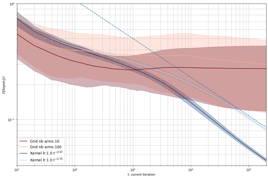
   Figure 1. Expected average regret, averaged on 92 realizations for each algorithm (solid line). The variance is presented (shaded area) where we add and remove the standard deviation (computed on the 92 seeds) from the mean. Finally, the theoretical regret bound is displayed (dashed line).

   

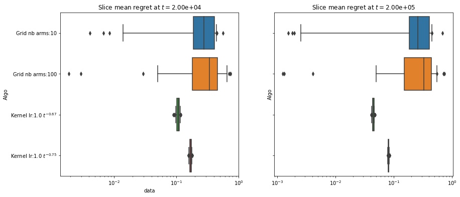
   Figure 2. Two slices of the mean regret, averaged on 92 realizations for each algorithm (solid line). Whisker at 5-95% CI , boxes at 25-75% CI and median displayed with vertical bars.

   The dashed line represent in the figure corresponds to the theoretical regret bound of $T^{-\frac{1}{3}}$, which is the expected regret bound of the Kernel algorithm mean regret (without explicit exploration in our case). For performance evaluation purposes, we “slice” different snapshots of the regret in Fig. 2 at iteration counts $2\times 10^{5}$ and $2\times 10^{5}$. In both cases, we observe a dramatic drop in variance for the Kernel algorithm relative to the Grid strategy, with a fixed number of arms uniformly cut beforehand; we also note that the performance of the Kernel method approaches the theoretical slope of $T^{-1/3}$ that characterizes the Kernel method.

   By contrast, the mean regret for the Grid approach seems to converge to a finite value which indicates a much slower regret minimization rate; on the other hand, the mean regret of the Kernel method converges to $0$ at the anticipated rate.

References

• Abernethy et al. [2008] Jacob Abernethy, Peter L. Bartlett, Alexander Rakhlin, and Ambuj Tewari. Optimal strategies and minimax lower bounds for online convex games. In COLT ’08: Proceedings of the 21st Annual Conference on Learning Theory, 2008.
• Agarwal et al. [2019] Naman Agarwal, Alon Gonen, and Elad Hazan. Learning in non-convex games with an optimization oracle. In COLT ’19: Proceedings of the 32nd Annual Conference on Learning Theory, 2019.
• Agrawal [1995] Rajeev Agrawal. Sample mean based index policies with $o(\log n)$ regret for the multi-armed bandit problem. Advances in Applied Probability, 27(4):1054–1078, December 1995.
• Alvarez et al. [2004] Felipe Alvarez, Jérôme Bolte, and Olivier Brahic. Hessian Riemannian gradient flows in convex programming. SIAM Journal on Control and Optimization, 43(2):477–501, 2004.
• Arora et al. [2012] Sanjeev Arora, Elad Hazan, and Satyen Kale. The multiplicative weights update method: A meta-algorithm and applications. Theory of Computing, 8(1):121–164, 2012.
• Auer et al. [1995] Peter Auer, Nicolò Cesa-Bianchi, Yoav Freund, and Robert E. Schapire. Gambling in a rigged casino: The adversarial multi-armed bandit problem. In Proceedings of the 36th Annual Symposium on Foundations of Computer Science, 1995.
• Auer et al. [2002a] Peter Auer, Nicolò Cesa-Bianchi, and Paul Fischer. Finite-time analysis of the multiarmed bandit problem. Machine Learning, 47:235–256, 2002a.
• Auer et al. [2002b] Peter Auer, Nicolò Cesa-Bianchi, Yoav Freund, and Robert E. Schapire. The nonstochastic multiarmed bandit problem. SIAM Journal on Computing, 32(1):48–77, 2002b.
• Balasundaram et al. [2011] Balabhaskar Balasundaram, Sergiy Butenko, and Illya V. Hicks. Clique relaxations in social network analysis: The maximum $k$-plex problem. Operations Research, 59(1):133–142, January 2011.
• Berge [1997] Claude Berge. Topological Spaces. Dover, New York, 1997.
• Besbes et al. [2015] Omar Besbes, Yonatan Gur, and Assaf Zeevi. Non-stationary stochastic optimization. Operations Research, 63(5):1227–1244, October 2015.
• Blum & Kalai [1999] Avrim Blum and Adam Tauman Kalai. Universal portfolios with and without transaction costs. Machine Learning, 35(3):193–205, 1999.
• Bomze et al. [1999] Immanuel M. Bomze, Marco Budinich, Panos M. Pardalos, and Marcello Pelillo. The maximum clique problem. In Handbook of Combinatorial Optimization. Springer, 1999.
• Bravo & Mertikopoulos [2017] Mario Bravo and Panayotis Mertikopoulos. On the robustness of learning in games with stochastically perturbed payoff observations. Games and Economic Behavior, 103, John Nash Memorial issue:41–66, May 2017.
• Bubeck [2015] Sébastien Bubeck. Convex optimization: Algorithms and complexity. Foundations and Trends in Machine Learning, 8(3-4):231–358, 2015.
• Bubeck & Cesa-Bianchi [2012] Sébastien Bubeck and Nicolò Cesa-Bianchi. Regret analysis of stochastic and nonstochastic multi-armed bandit problems. Foundations and Trends in Machine Learning, 5(1):1–122, 2012.
• Bubeck & Eldan [2016] Sébastien Bubeck and Ronen Eldan. Multi-scale exploration of convex functions and bandit convex optimization. In COLT ’16: Proceedings of the 29th Annual Conference on Learning Theory, 2016.
• Bubeck et al. [2011] Sébastien Bubeck, Rémi Munos, Gilles Stoltz, and Csaba Szepesvári. $\mathcal{X}$-armed bandits. Journal of Machine Learning Research, 12:1655–1695, 2011.
• Bubeck et al. [2017] Sébastien Bubeck, Yin Tat Lee, and Ronen Eldan. Kernel-based methods for bandit convex optimization. In STOC ’17: Proceedings of the 49th annual ACM SIGACT symposium on the Theory of Computing, 2017.
• Cesa-Bianchi & Lugosi [2006] Nicolò Cesa-Bianchi and Gábor Lugosi. Prediction, Learning, and Games. Cambridge University Press, 2006.
• Cesa-Bianchi et al. [2012] Nicolò Cesa-Bianchi, Pierre Gaillard, Gábor Lugosi, and Gilles Stoltz. Mirror descent meets fixed share (and feels no regret). In 989-997 (ed.), Advances in Neural Information Processing Systems, volume 25, 2012.
• Chen & Teboulle [1993] Gong Chen and Marc Teboulle. Convergence analysis of a proximal-like minimization algorithm using Bregman functions. SIAM Journal on Optimization, 3(3):538–543, August 1993.
• Chiang et al. [2012] Chao-Kai Chiang, Tianbao Yang, Chia-Jung Lee, Mehrdad Mahdavi, Chi-Jen Lu, Rong Jin, and Shenghuo Zhu. Online optimization with gradual variations. In COLT ’12: Proceedings of the 25th Annual Conference on Learning Theory, 2012.
• Duvocelle et al. [2018] Benoit Duvocelle, Panayotis Mertikopoulos, Mathias Staudigl, and Dries Vermeulen. Learning in time-varying games. https://arxiv.org/abs/1809.03066, 2018.
• Flaxman et al. [2005] Abraham D. Flaxman, Adam Tauman Kalai, and H. Brendan McMahan. Online convex optimization in the bandit setting: gradient descent without a gradient. In SODA ’05: Proceedings of the 16th annual ACM-SIAM Symposium on Discrete Algorithms, pp.  385–394, 2005.
• Folland [1999] Gerald B. Folland. Real Analysis. Wiley-Interscience, 2 edition, 1999.
• Fortunato [2010] Santo Fortunato. Community detection in graphs. Physics Reports, 486(3-5):75–174, 2010.
• Hallak et al. [2020] Nadav Hallak, Panayotis Mertikopoulos, and Volkan Cevher. Regret minimization in stochastic non-convex learning via a proximal-gradient approach. https://arxiv.org/abs/2010.06250, 2020.
• Hazan [2012] Elad Hazan. A survey: The convex optimization approach to regret minimization. In Suvrit Sra, Sebastian Nowozin, and Stephen J. Wright (eds.), Optimization for Machine Learning, pp.  287–304. MIT Press, 2012.
• Hazan & Seshadhri [2009] Elad Hazan and Comandur Seshadhri. Efficient learning algorithms for changing environments. In ICML ’09: Proceedings of the 26th International Conference on Machine Learning, 2009.
• Hazan et al. [2017] Elad Hazan, Karan Singh, and Cyril Zhang. Efficient regret minimization in non-convex games. In ICML ’17: Proceedings of the 34th International Conference on Machine Learning, 2017.
• Herbster & Warmuth [1998] Mark Herbster and Manfred K. Warmuth. Tracking the best expert. Machine Learning, 32(2):151–178, 1998.
• Jadbabaie et al. [2015] Ali Jadbabaie, Alexander Rakhlin, Shahin Shahrampour, and Karthik Sridharan. Online optimization: Competing with dynamic comparators. In AISTATS ’15: Proceedings of the 18th International Conference on Artificial Intelligence and Statistics, 2015.
• Kalai & Vempala [2005] Adam Tauman Kalai and Santosh Vempala. Efficient algorithms for online decision problems. Journal of Computer and System Sciences, 71(3):291–307, October 2005.
• Karmarkar [1990] Narendra Karmarkar. Riemannian geometry underlying interior point methods for linear programming. In Mathematical Developments Arising from Linear Programming, number 114 in Contemporary Mathematics. American Mathematical Society, 1990.
• Kleinberg [2004] Robert David Kleinberg. Nearly tight bounds for the continuum-armed bandit problem. In NIPS’ 04: Proceedings of the 18th Annual Conference on Neural Information Processing Systems, 2004.
• Kleinberg et al. [2008] Robert David Kleinberg, Aleksandrs Slivkins, and Eli Upfal. Multi-armed bandits in metric spaces. In STOC ’08: Proceedings of the 40th annual ACM symposium on the Theory of Computing, 2008.
• Krichene et al. [2015] Walid Krichene, Maximilian Balandat, Claire Tomlin, and Alexandre Bayen. The Hedge algorithm on a continuum. In ICML ’15: Proceedings of the 32nd International Conference on Machine Learning, 2015.
• Littlestone & Warmuth [1994] Nick Littlestone and Manfred K. Warmuth. The weighted majority algorithm. Information and Computation, 108(2):212–261, 1994.
• Mertikopoulos & Zhou [2019] Panayotis Mertikopoulos and Zhengyuan Zhou. Learning in games with continuous action sets and unknown payoff functions. Mathematical Programming, 173(1-2):465–507, January 2019.
• Motzkin & Straus [1965] Theodore S. Motzkin and Ernst G. Straus. Maxima for graphs and a new proof of a theorem of Turán. Canadian Journal of Mathematics, 1965.
• Nesterov [2009] Yurii Nesterov. Primal-dual subgradient methods for convex problems. Mathematical Programming, 120(1):221–259, 2009.
• Perkins et al. [2017] Steven Perkins, Panayotis Mertikopoulos, and David S. Leslie. Mixed-strategy learning with continuous action sets. IEEE Trans. Autom. Control, 62(1):379–384, January 2017.
• Phelps [1993] Robert Ralph Phelps. Convex Functions, Monotone Operators and Differentiability. Lecture Notes in Mathematics. Springer-Verlag, 2 edition, 1993.
• Shalev-Shwartz [2011] Shai Shalev-Shwartz. Online learning and online convex optimization. Foundations and Trends in Machine Learning, 4(2):107–194, 2011.
• Shalev-Shwartz & Singer [2007] Shai Shalev-Shwartz and Yoram Singer. Convex repeated games and Fenchel duality. In Advances in Neural Information Processing Systems 19, pp. 1265–1272. MIT Press, 2007.
• Slivkins [2019a] Aleksandrs Slivkins. Introduction to multi-armed bandits. arXiv preprint arXiv:1904.07272, 2019a.
• Slivkins [2019b] Aleksandrs Slivkins. Introduction to multi-armed bandits. Foundations and Trends in Machine Learning, 12(1-2):1–286, November 2019b.
• Spirin & Mirny [2003] Victor Spirin and Leonid A. Mirny. Protein complexes and functional modules in molecular networks. Proceedings of the National Academy of Sciences, 2003.
• Suggala & Netrapalli [2020] Arun Sai Suggala and Praneeth Netrapalli. Online non-convex learning: Following the perturbed leader is optimal. In ALT ’20: Proceedings of the 31st International Conference on Algorithmic Learning Theory, 2020.
• Tsallis [1988] Constantino Tsallis. Possible generalization of Boltzmann–Gibbs statistics. Journal of Statistical Physics, 52:479–487, 1988.
• Tseng [2004] Paul Tseng. Convergence properties of Dikin’s affine scaling algorithm for nonconvex quadratic minimization. Journal of Global Optimization, 30(2):285–300, 2004.
• Vanderbei et al. [1986] Robert J. Vanderbei, Marc S. Meketon, and Barry A. Freedman. A modification of Karmarkar’s linear programming algorithm. Algorithmica, 1(1):395–407, November 1986.
• Vovk [1990] Vladimir G. Vovk. Aggregating strategies. In COLT ’90: Proceedings of the 3rd Workshop on Computational Learning Theory, pp.  371–383, 1990.
• Xiao [2010] Lin Xiao. Dual averaging methods for regularized stochastic learning and online optimization. Journal of Machine Learning Research, 11:2543–2596, October 2010.
• Zhong et al. [2018] Zhisheng Zhong, Tiancheng Shen, Yibo Yang, Chao Zhang, and Zhouchen Lin. Joint sub-bands learning with clique structures for wavelet domain super-resolution. In NeurIPS ’18: Proceedings of the 32nd International Conference of Neural Information Processing Systems, 2018.
• Zhou et al. [2020] Zhengyuan Zhou, Panayotis Mertikopoulos, Nicholas Bambos, Stephen P. Boyd, and Peter W. Glynn. On the convergence of mirror descent beyond stochastic convex programming. SIAM Journal on Optimization, 30(1):687–716, 2020.
• Zinkevich [2003] Martin Zinkevich. Online convex programming and generalized infinitesimal gradient ascent. In ICML ’03: Proceedings of the 20th International Conference on Machine Learning, pp.  928–936, 2003.