EUROPEAN ORGANIZATION FOR NUCLEAR RESEARCH (CERN)

​​​ CERN-EP-2020-175 LHCb-PAPER-2020-019

Measurement of the CKM angle $\gamma$

in $B^{\pm}\rightarrow DK^{\pm}$ and $B^{\pm}\rightarrow D\pi^{\pm}$ decays with $D\rightarrow K_{\mathrm{S}}^{0}h^{+}h^{-}$

LHCb collaboration

A measurement of $C\!P$-violating observables is performed using the decays ${{{B}^{\pm}}\rightarrow{D}{{K}^{\pm}}}$ and ${{{B}^{\pm}}\rightarrow{D}{{\pi}^{\pm}}}$, where the $D$ meson is reconstructed in one of the self-conjugate three-body final states ${{K}^{0}_{\mathrm{S}}}{{\pi}^{+}}{{\pi}^{-}}$ and ${{K}^{0}_{\mathrm{S}}}{{K}^{+}}{{K}^{-}}$ (commonly denoted ${{K}^{0}_{\mathrm{S}}}h^{+}h^{-}$). The decays are analysed in bins of the $D$-decay phase space, leading to a measurement that is independent of the modelling of the $D$-decay amplitude. The observables are interpreted in terms of the CKM angle $\gamma$. Using a data sample corresponding to an integrated luminosity of 9$\text{\,fb}^{-1}$ collected in proton-proton collisions at centre-of mass energies of $7$, $8$, and $13\text{\,Te\kern-1.00006ptV}$ with the LHCb experiment, $\gamma$ is measured to be $\left(68.7^{+5.2}_{-5.1}\right)^{\circ}$. The hadronic parameters $r_{B}^{{D}{K}}$, $r_{B}^{{D}\pi}$, $\delta_{B}^{{D}{K}}$, and $\delta_{B}^{{D}\pi}$, which are the ratios and strong-phase differences of the suppressed and favoured ${B}^{\pm}$ decays, are also reported.

Published in J. High Energ. Phys. 2021, 169 (2021).

© 2024 CERN for the benefit of the LHCb collaboration. CC BY 4.0 licence.

 

1 Introduction

In the framework of the Standard Model, $C\!P$ violation can be described by the angles and lengths of the Unitarity Triangle constructed from elements of the CKM matrix [1, 2]. The angle $\gamma\equiv\textrm{arg}\left(-{V_{{u}{d}}^{\phantom{\ast}}}{V_{{u}{b}}^{\ast}}/{V_{{c}{d}}^{\phantom{\ast}}}{V_{{c}{b}}^{\ast}}\right)$ has particularly interesting features. It is the only CKM angle that can be measured in decays including only tree-level processes, and is experimentally accessible through the interference of ${\overline{b}}\rightarrow{\overline{c}}{u}{\overline{s}}$ and ${\overline{b}}\rightarrow{\overline{u}}{c}{\overline{s}}$ (and $C\!P$-conjugate) decay amplitudes. In addition, there are negligible theoretical uncertainties when interpreting the measured observables in terms of $\gamma$ [3]. Hence, in the absence of unknown physics effects at tree level, a precision measurement of $\gamma$ provides a Standard Model benchmark that can be compared with indirect determinations from other CKM-matrix observables more likely to be affected by physics beyond the Standard Model [4]. Such comparisons are currently limited by the precision of direct measurements of $\gamma$, which is about $5^{\circ}$ [5, 6] dominated by LHCb results.

Decays such as ${{{B}^{\pm}}\rightarrow{D}{{K}^{\pm}}}$, where $D$ represents a superposition of ${D}^{0}$ and ${\kern 1.79993pt\overline{\kern-1.79993ptD}}{}^{0}$ states, are used to observe the effects of interference between ${\overline{b}}\rightarrow{\overline{c}}{u}{\overline{s}}$ and ${\overline{b}}\rightarrow{\overline{u}}{c}{\overline{s}}$ (and $C\!P$-conjugate) decay amplitudes. The interference arises when the decay channel of the $D$ meson is common to both ${D}^{0}$ and ${\kern 1.79993pt\overline{\kern-1.79993ptD}}{}^{0}$ mesons. The ${{{B}^{\pm}}\rightarrow{D}{{K}^{\pm}}}$ decay has been studied extensively with a wide range of $D$-meson final states [7, 8, 9, 10, 11]. The exact choice of observables from each of these analyses is dependent on the method that is most appropriate for the $D$ decay used [12, 13, 14, 15, 16, 17, 18, 19, 20]. The methods can be extended to a variety of different $B$-decay modes [8, 21, 22, 23, 24].

This paper presents a model-independent study of the decay modes ${{{B}^{\pm}}\rightarrow{D}{{K}^{\pm}}}$ and ${{{B}^{\pm}}\rightarrow{D}{{\pi}^{\pm}}}$ where the chosen $D$ decays are the self-conjugate decays ${D}\rightarrow{{K}^{0}_{\mathrm{S}}}{{\pi}^{+}}{{\pi}^{-}}$ and ${D}\rightarrow{{K}^{0}_{\mathrm{S}}}{{K}^{+}}{{K}^{-}}$ (denoted ${D}\rightarrow{{K}^{0}_{\mathrm{S}}}{h}^{+}{h}^{-}$). The analysis of the ${{{B}^{\pm}}\rightarrow{D}{{K}^{\pm}}}$, ${D}\rightarrow{{K}^{0}_{\mathrm{S}}}{h}^{+}{h}^{-}$ decay chain is powerful due to the rich resonance structure of the $D$-decay modes, as has been described in Refs. [18, 17, 19]. The data used in this analysis were accumulated with the LHCb detector over the period 2011–2018 in $pp$ collisions at energies of $\sqrt{s}$ =7, 8, 13  TeV, corresponding to a total integrated luminosity of approximately 9$\text{\,fb}^{-1}$.

The presence of interference leads to differences in the phase-space distributions of $D$ decays from reconstructed ${{B}^{+}}$ and ${{B}^{-}}$ decays. In order to interpret any observed difference in the context of the angle $\gamma$, knowledge of the strong phase of the ${D}^{0}$ decay amplitude, and how it varies over phase space, is required. An attractive model-independent approach makes use of direct measurements of the strong-phase difference between ${D}^{0}$ and ${\kern 1.79993pt\overline{\kern-1.79993ptD}}{}^{0}$ decays, averaged over regions of the phase space [17, 25, 26]. Quantum correlated pairs of $D$ mesons produced in decays of $\psi(3770)$ give direct access to the strong-phase differences. These have been measured by the CLEO collaboration [27], and more recently the BESIII collaboration [28, 29, 30]. Measurements using the inputs in Ref. [27] have been used by the LHCb [10, 21, 31] and Belle [32, 33] collaborations. An alternate method is to use an amplitude model of the $D$ decay to determine the strong-phase variation [34, 35, 36]. The separation of data into binned regions of the Dalitz plot leads to a loss of statistical sensitivity in comparison to using an amplitude model. However, the advantage of using the direct strong-phase measurements resides in the model-independent nature of the systematic uncertainties. Where the direct strong-phase measurements are used, there is only a systematic uncertainty associated with the finite precision of such measurements. Conversely, systematic uncertainties associated with determining a phase from an amplitude model are difficult to evaluate, as common approaches to amplitude-model building violate the optical theorem [37]. Therefore, the loss in statistical precision is compensated by reliability in the evaluation of the systematic uncertainty, which is increasingly important as the overall precision on the CKM angle $\gamma$ improves. The analysis approach is laid out in Sect. 2, while Sect. 3 describes the LHCb detector used to collect the data sample, and Sect. 4 summarises the selection criteria. The measurement is based on a two-step fit procedure covered in Sect. 5, where the fit to the invariant-mass distribution is detailed, and Sect. 6, which describes how the $C\!P$ observables are determined. The systematic uncertainties are reported in Sect. 7, and the results are interpreted to determine the value of $\gamma$ in Sect. 8. Finally, the conclusions are presented in Sect. 9.

2 Analysis Overview

The sum of the favoured and suppressed contributions to the ${{{B}^{-}}}\rightarrow{D}{{K}^{-}}$ amplitude can be written as

$$A_{B}(m^{2}_{-},m^{2}_{+})\propto\,A_{D}(m^{2}_{-},m^{2}_{+})+r_{B}^{{D}{K}}e^{i(\delta_{B}^{{D}{K}}-\gamma)}A_{{\kern 1.25995pt\overline{\kern-1.25995ptD}}}(m^{2}_{-},m^{2}_{+}),$$ (1)

where $A_{D}(m^{2}_{-},m^{2}_{+})$ is the ${{D}^{0}}\rightarrow{{K}^{0}_{\mathrm{S}}}h^{+}h^{-}$ decay amplitude, and $A_{{\kern 1.25995pt\overline{\kern-1.25995ptD}}}(m^{2}_{-},m^{2}_{+})$ is the ${{{\kern 1.79993pt\overline{\kern-1.79993ptD}}{}^{0}}\rightarrow{{K}^{0}_{\mathrm{S}}}h^{+}h^{-}}$ decay amplitude. The hadronic parameters $r_{B}^{{D}{K}}$ and $\delta_{B}^{{D}{K}}$ are the ratio of the magnitudes of the amplitudes of ${{{B}^{-}}}\rightarrow{{\kern 1.79993pt\overline{\kern-1.79993ptD}}{}^{0}}{{K}^{-}}$ and ${{{B}^{-}}}\rightarrow{{D}^{0}}{{K}^{-}}$ and the strong-phase difference between them, respectively. Finally, the position of the decay in the Dalitz plot is defined by $m^{2}_{-}$ and $m^{2}_{+}$, which are the squared invariant masses of the ${{K}^{0}_{\mathrm{S}}}h^{-}$ and ${{K}^{0}_{\mathrm{S}}}h^{+}$ particle combinations, respectively. The equivalent expression for the charge-conjugated decay $B^{+}\rightarrow DK^{+}$ is obtained by making the substitutions $\gamma\rightarrow-\gamma$ and $A_{D}(m^{2}_{-},m^{2}_{+})\leftrightarrow A_{{\kern 1.25995pt\overline{\kern-1.25995ptD}}}(m^{2}_{-},m^{2}_{+})$.

The $D$-decay phase space is partitioned into $2\times\mathcal{N}$ bins labelled from $i=-\mathcal{N}$ to $i=+\mathcal{N}$ (excluding zero), symmetric around $m^{2}_{-}=m^{2}_{+}$ such that if $(m^{2}_{-},m^{2}_{+})$ is in bin $i$ then $(m^{2}_{+},m^{2}_{-})$ is in bin $-i$. The bins for which $m^{2}_{-}>m^{2}_{+}$ are defined to have positive values of $i$. The strong-phase difference between the ${D}^{0}$- and ${\kern 1.79993pt\overline{\kern-1.79993ptD}}{}^{0}$-decay amplitudes at a given point on the Dalitz plot is denoted as $\delta_{D}(m_{-}^{2},m_{+}^{2})$. The cosine of $\delta_{D}(m_{-}^{2},m_{+}^{2})$ weighted by the $D$-decay amplitude and averaged over bin $i$ is written as $c_{i}$ [17], and is given by

$$c_{i} \equiv\frac{\int_{i}dm^{2}_{-}\,dm^{2}_{+}\,|A_{D}(m^{2}_{-},m^{2}_{+})||A_{D}(m^{2}_{+},m^{2}_{-})|\cos\ [\delta_{D}(m^{2}_{-},m^{2}_{+})-\delta_{D}(m^{2}_{+},m^{2}_{-})]}{\sqrt{\int_{i}dm^{2}_{-}\,dm^{2}_{+}\,|A_{D}(m^{2}_{-},m^{2}_{+})|^{2}\int_{i}dm^{2}_{-}\,dm^{2}_{+}\,|A_{D}(m^{2}_{+},m^{2}_{-})|^{2}}}\,,$$ (2)

where the integrals are evaluated over bin $i$. An analogous expression can be written for $s_{i}$, which is the sine of the strong-phase difference weighted by the decay amplitude and averaged over the bin phase space.

The expected yield of ${{B}^{-}}$ decays in bin $i$ is found by integrating the square of the amplitude given in Eq. (1) over the region of phase space defined by the $i$th bin. The effects of charm mixing and $C\!P$ violation are ignored, as is the presence of $C\!P$ violation and matter regeneration in the neutral $K^{0}$ decays. These effects are expected to have a small impact [38, 39] on the distribution of events on the Dalitz plot. Selection requirements and reconstruction effects lead to a non-uniform efficiency over phase space, denoted by $\eta(m^{2}_{-},m^{2}_{+})$. At LHCb the typical efficiency variation over phase space for a ${D}\rightarrow{{K}^{0}_{\mathrm{S}}}{h}^{+}{h}^{-}$ decay from a region of high efficiency to low efficiency is approximately 60% [21]. The fractional yield of pure ${D}^{0}$ decays in bin $i$ in the presence of this efficiency profile is denoted $F_{i}$, given by

$$F_{i}=\frac{\int_{i}dm^{2}_{-}dm^{2}_{+}|A_{D}(m^{2}_{-},m^{2}_{+})|^{2}\,\eta(m^{2}_{-},m^{2}_{+})}{\sum_{j}\int_{j}dm^{2}_{-}dm^{2}_{+}|A_{D}(m^{2}_{-},m^{2}_{+})|^{2}\,\eta(m^{2}_{-},m^{2}_{+})},$$ (3)

where the sum in the denominator is over all Dalitz plot bins, indexed by $j$. Neglecting $C\!P$ violation in these charm decays, the charge-conjugate amplitudes satisfy the relation $A_{{\kern 1.25995pt\overline{\kern-1.25995ptD}}}(m^{2}_{-},m^{2}_{+})=A_{D}(m^{2}_{+},m^{2}_{-})$, and therefore $F_{i}$ = $\overline{F}_{-i}$, where $\overline{F}_{i}$ is the fractional yield of ${\kern 1.79993pt\overline{\kern-1.79993ptD}}{}^{0}$ decays to bin $i$. The physics parameters of interest, $r_{B}^{{D}{K}}$, $\delta_{B}^{{D}{K}}$, and $\gamma$, are translated into four $C\!P$-violating observables [40] that are measured in this analysis and are the real and imaginary parts of the ratio of the suppressed and favoured $B$ decay amplitudes,

$$x_{\pm}^{{D}{K}}\equiv r_{B}^{{D}{K}}\cos(\delta_{B}^{{D}{K}}\pm\gamma){\rm\ \ and\ }\;y_{\pm}^{{D}{K}}\equiv r_{B}^{{D}{K}}\sin(\delta_{B}^{{D}{K}}\pm\gamma).$$ (4)

Using the relations $c_{i}=c_{-i}$ and $s_{i}=-s_{-i}$ the ${{B}^{+}}$ (${{B}^{-}}$) yields, $N^{+}$ ($N^{-}$), in bin $i$ and $-i$ are given by

$$\begin{split}N_{+i}^{+}&=h_{B^{+}}\left[F_{-i}+\left(\left(x_{+}^{{D}{K}}\right)^{2}+\left(y_{+}^{{D}{K}}\right)^{2}\right)F_{+i}+2\sqrt{F_{i}F_{-i}}\left(x_{+}^{{D}{K}}c_{+i}-y_{+}^{{D}{K}}s_{+i}\right)\right],\\ N_{-i}^{+}&=h_{B^{+}}\left[F_{+i}+\left(\left(x_{+}^{{D}{K}}\right)^{2}+\left(y_{+}^{{D}{K}}\right)^{2}\right)F_{-i}+2\sqrt{F_{i}F_{-i}}\left(x_{+}^{{D}{K}}c_{+i}+y_{+}^{{D}{K}}s_{+i}\right)\right],\\ N_{+i}^{-}&=h_{B^{-}}\left[F_{+i}+\left(\left(x_{-}^{{D}{K}}\right)^{2}+\left(y_{-}^{{D}{K}}\right)^{2}\right)F_{-i}+2\sqrt{F_{i}F_{-i}}\left(x_{-}^{{D}{K}}c_{+i}+y_{-}^{{D}{K}}s_{+i}\right)\right],\\ N_{-i}^{-}&=h_{B^{-}}\left[F_{-i}+\left(\left(x_{-}^{{D}{K}}\right)^{2}+\left(y_{-}^{{D}{K}}\right)^{2}\right)F_{+i}+2\sqrt{F_{i}F_{-i}}\left(x_{-}^{{D}{K}}c_{+i}-y_{-}^{{D}{K}}s_{+i}\right)\right],\end{split}$$ (5)

where $h_{B^{+}}$ and $h_{B^{-}}$ are normalisation constants. The value of $r_{B}^{{D}{K}}$ is allowed to be different for each charge and is constructed from either $(r_{B}^{{D}{K}})^{2}=\left(x_{+}^{{D}{K}}\right)^{2}+\left(y_{+}^{{D}{K}}\right)^{2}$ or $(r_{B}^{{D}{K}})^{2}=\left(x_{-}^{{D}{K}}\right)^{2}+\left(y_{-}^{{D}{K}}\right)^{2}$. A single value of $r_{B}^{{D}{K}}$ is determined when the $C\!P$ observables are subsequently interpreted to determine the physics parameters of interest. The normalisation constants can be written as a function of $\gamma$, analogous to the global asymmetries studied in decays where the $D$ meson decays to a $C\!P$ eigenstate [8]. However, not only is this global asymmetry expected to be small since the $C\!P$-even content of the ${D}\rightarrow{{K}^{0}_{\mathrm{S}}}{{\pi}^{+}}{{\pi}^{-}}$ and ${D}\rightarrow{{K}^{0}_{\mathrm{S}}}{{K}^{+}}{{K}^{-}}$ decay modes is close to 0.5, it is also expected to be heavily biased due to the effects of ${{K}^{0}_{\mathrm{S}}}$ $C\!P$ violation [39] on total yields. Therefore the global asymmetry is ignored and the loss of information is minimal. An advantage of this approach is that the normalisation constants $h_{{{{B}^{+}}}}$ and $h_{{{{B}^{-}}}}$ are independent of each other, and will implicitly contain the effects of the production asymmetry of ${B}^{\pm}$ mesons in $pp$ collisions and the detection asymmetries of the charged kaon from the $B$ decay. This leads to a $C\!P$-violation measurement that is free of systematic uncertainties associated to these effects.

The system of equations provides $4\mathcal{N}$ observables and $4+2\mathcal{N}$ unknowns, assuming that the available measurements of $c_{i}$ and $s_{i}$ are used. This is solvable for $\mathcal{N}\geq 2$, but in practice the simultaneous fit of the $F_{i}$, $x_{\pm}^{{D}{K}}$, and $y_{\pm}^{{D}{K}}$ parameters leads to large uncertainties on the $C\!P$ observables, and hence some external knowledge of the $F_{i}$ parameters is desirable. The $F_{i}$ parameters could be computed from simulation and an amplitude model, but the systematic uncertainties associated with the LHCb simulation would be significant. Recent analyses [31, 10] have used the semileptonic decay $B\rightarrow{D}^{*}\mu\nu$, where the flavour-tagged yields of ${D}^{0}$ mesons are corrected for the differences in selection between the semileptonic channel and the signal mode. However, with the increased signal yields, the uncertainty due to this necessary correction will be approximately half the statistical uncertainty on the measurement presented in this paper, and therefore a different method is adopted.

The ${{{B}^{\pm}}\rightarrow{D}{{\pi}^{\pm}}}$ decay mode is expected to have $F_{i}$ parameters that are the same as those for ${{{B}^{\pm}}\rightarrow{D}{{K}^{\pm}}}$ if a similar selection is applied due to the common topology and the ability to use same signatures in the detector to select the candidates. The ${{{B}^{\pm}}\rightarrow{D}{{\pi}^{\pm}}}$ decay is expected to exhibit $C\!P$ violation through the interference of ${\overline{b}}\rightarrow{\overline{c}}{u}{\overline{d}}$ and ${\overline{b}}\rightarrow{\overline{u}}{c}{\overline{d}}$ transitions, analogous to the ${{{B}^{\pm}}\rightarrow{D}{{K}^{\pm}}}$ decay but suppressed by one order of magnitude [41]. Further effects from ${{K}^{0}_{\mathrm{S}}}$ $C\!P$ violation and matter regeneration have been recently shown to have only a small impact on the distribution over the Dalitz plot [39], in contrast to their impact on the global asymmetry. Therefore the ${{{B}^{\pm}}\rightarrow{D}{{\pi}^{\pm}}}$ channel can be used to determine the $F_{i}$ parameters if the small level of $C\!P$ violation in the ${B}^{\pm}$ decay is accounted for.

Pseudoexperiments are performed in which the two $B$-decay modes are fit together assuming common $F_{i}$ parameters. Independent $x_{\pm}$ and $y_{\pm}$ observables are required for the two $B$ decay modes due to different values of the hadronic parameters, $r_{B}$ and $\delta_{B}$. The value of $r_{B}$ in ${{{B}^{\pm}}\rightarrow{D}{{K}^{\pm}}}$ is approximately $0.1$, and it is expected that it will be a factor 20 smaller in ${{{B}^{\pm}}\rightarrow{D}{{\pi}^{\pm}}}$ decays [41]. The yields of ${{{B}^{\pm}}\rightarrow{D}{{\pi}^{\pm}}}$ are described by a set of equations analogous to Eq. (5), with the substitutions $x_{\pm}^{{D}{K}}\rightarrow x_{\pm}^{{D}\pi}$ and $y_{\pm}^{{D}{K}}\rightarrow y_{\pm}^{{D}\pi}$. An analysis that simultaneously measures the $F_{i}$, $x_{\pm}^{{D}{K}}$, $y_{\pm}^{{D}{K}}$, $x_{\pm}^{{D}\pi}$, and $y_{\pm}^{{D}\pi}$ parameters is found to be stable only if $r_{B}^{{D}\pi}>0.03$. At the expected value $r_{B}^{{D}\pi}=0.005$ the fit is unstable due to high correlations between the $F_{i}$ and $x_{\pm}^{{D}\pi}$ and $y_{\pm}^{{D}\pi}$. Therefore an alternate parameterisation [42, 43] is introduced, which utilises the fact that $\gamma$ is a common parameter, and that the $C\!P$ violation in ${{{B}^{\pm}}\rightarrow{D}{{\pi}^{\pm}}}$ decays can therefore be described by the addition of a single complex variable

$$\xi^{{D}\pi}=\left(\frac{r_{B}^{{D}\pi}}{r_{B}^{{D}{K}}}\right)\exp{\left(i\delta_{B}^{{D}\pi}-i\delta_{B}^{{D}{K}}\right)},$$ (6)

and in terms of $x_{\xi}^{{D}\pi}\equiv\text{Re}(\xi^{{D}\pi})$ and $y_{\xi}^{{D}\pi}\equiv\text{Im}(\xi^{{D}\pi})$, the $\left(x_{\pm}^{{D}\pi},y_{\pm}^{{D}\pi}\right)$ parameters are given by

$$x_{\pm}^{{D}\pi} =x_{\xi}^{{D}\pi}x_{\pm}^{{D}{K}}-y_{\xi}^{{D}\pi}y_{\pm}^{{D}{K}}, y_{\pm}^{{D}\pi} =x_{\xi}^{{D}\pi}y_{\pm}^{{D}{K}}+y_{\xi}^{{D}\pi}x_{\pm}^{{D}{K}}.$$ (7)

With this parameterisation, the simultaneous fit to $x_{\pm}^{{D}{K}}$, $y_{\pm}^{{D}{K}}$, $x_{\xi}^{{D}\pi}$, $y_{\xi}^{{D}\pi}$ (the $C\!P$ observables) and $F_{i}$ parameters is stable for all values of $r_{B}^{{D}\pi}$. The simultaneous fit of ${{{B}^{\pm}}\rightarrow{D}{{\pi}^{\pm}}}$ and ${{{B}^{\pm}}\rightarrow{D}{{K}^{\pm}}}$ candidates has two advantages. Firstly, the extraction of $F_{i}$ in this manner is expected to have negligible associated systematic uncertainty, and reduces significantly the reliance on simulation. Secondly, the $C\!P$-violating observables in ${{{B}^{\pm}}\rightarrow{D}{{\pi}^{\pm}}}$ using other $D$-decay modes [8, 9] are not routinely included in the $\gamma$ combination of all results because they allow for two solutions of $\left(r_{B}^{{D}\pi},\delta_{B}^{{D}\pi}\right)$, which makes the statistical interpretation of the full ${{B}^{\pm}}\rightarrow{D}{h}^{\pm}$ combination problematic [44]. The measurement in the ${{{B}^{\pm}}\rightarrow{D}{{\pi}^{\pm}}}$, ${D}\rightarrow{{K}^{0}_{\mathrm{S}}}{h}^{+}{h}^{-}$ decays has the potential to resolve this redundancy, and allow for a more straightforward inclusion of all ${{{B}^{\pm}}\rightarrow{D}{{\pi}^{\pm}}}$ results in the combination. A small disadvantage is that the measurement of $\gamma$ will incorporate information from both ${{{B}^{\pm}}\rightarrow{D}{{K}^{\pm}}}$ and ${{{B}^{\pm}}\rightarrow{D}{{\pi}^{\pm}}}$ decay modes and the contribution of each cannot be disentangled. However, since the size of contribution from the ${{{B}^{\pm}}\rightarrow{D}{{\pi}^{\pm}}}$ decay to the precision is expected to be negligible in comparison to that from the ${{{B}^{\pm}}\rightarrow{D}{{K}^{\pm}}}$ decay, this is considered an acceptable compromise.

The measurements of $c_{i}$ and $s_{i}$ are available in four different $2\times 8$ binning schemes for the ${D}\rightarrow{{K}^{0}_{\mathrm{S}}}{{\pi}^{+}}{{\pi}^{-}}$ decay. This analysis uses the scheme called the optimal binning, where the bins have been chosen to optimise the statistical sensitivity to $\gamma$, as described in Ref. [27]. The optimisation was performed assuming a strong-phase difference distribution as predicted by the BaBar model presented in Ref. [45]. For the ${{K}^{0}_{\mathrm{S}}}{{K}^{+}}{{K}^{-}}$ final state, three choices of binning schemes are available, containing $2\times 2$, $2\times 3$, and $2\times 4$ bins. The guiding model used to determine the bin boundaries is taken from the BaBar study described in Ref. [46]. The ${D}\rightarrow{{K}^{0}_{\mathrm{S}}}{{K}^{+}}{{K}^{-}}$ decay mode is dominated by the intermediate ${{K}^{0}_{\mathrm{S}}}\phi$ and ${{K}^{0}_{\mathrm{S}}}a(980)$ states which are $C\!P$-odd and $C\!P$-even, respectively, and the narrow ${{K}^{0}_{\mathrm{S}}}\phi$ resonance is encapsulated within the second bin of the $2\times 2$ scheme. Therefore, most of the sensitivity is encompassed by this scheme, and the additional small gains from the more detailed schemes are offset by low yields and fit instabilities that arise when these bins are used. Therefore, the $2\times 2$ bin is used for the analysis of the ${D}\rightarrow{{K}^{0}_{\mathrm{S}}}{{K}^{+}}{{K}^{-}}$ decay mode. The measurements of $c_{i}$ and $s_{i}$ are not biased by the use of a specific amplitude model in defining the bin boundaries. The choice of the model only affects this analysis to the extent that a poor model description of the underlying decay would result in a reduced statistical sensitivity of the $\gamma$ measurement. The binning choices for the two decay modes are shown in Fig. 1.

Measurements of the $c_{i}$ and $s_{i}$ parameters in the optimal binning scheme for the ${D}\rightarrow{{K}^{0}_{\mathrm{S}}}{{\pi}^{+}}{{\pi}^{-}}$ decay and in the $2\times 2$ binning scheme for the ${D}\rightarrow{{K}^{0}_{\mathrm{S}}}{{K}^{+}}{{K}^{-}}$ decay are available from both the CLEO and BESIII collaborations. A combination of results from both collaborations is presented in Ref. [29] and Ref. [30] for the ${D}\rightarrow{{K}^{0}_{\mathrm{S}}}{{\pi}^{+}}{{\pi}^{-}}$ and ${D}\rightarrow{{K}^{0}_{\mathrm{S}}}{{K}^{+}}{{K}^{-}}$ decays, respectively. The combinations are used within this analysis.

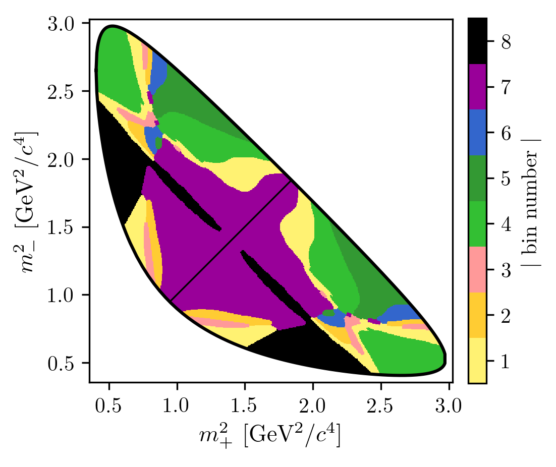
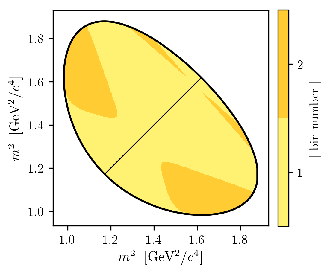
Figure 1: Binning schemes for (left) ${D}\rightarrow{{K}^{0}_{\mathrm{S}}}{{\pi}^{+}}{{\pi}^{-}}$ decays and (right) ${D}\rightarrow{{K}^{0}_{\mathrm{S}}}{{K}^{+}}{{K}^{-}}$ decays. The diagonal line separates the positive and negative bins, where the positive bins are in the region in which $m^{2}_{-}>m^{2}_{+}$ is satisfied.

3 LHCb Detector

The LHCb detector [47, 48] is a single-arm forward spectrometer covering the pseudorapidity range $2<\eta<5$, designed for the study of particles containing $b$ or $c$ quarks. The detector includes a high-precision tracking system consisting of a silicon-strip vertex detector surrounding the $pp$ interaction region, a large-area silicon-strip detector located upstream of a dipole magnet with a bending power of about $4{\mathrm{\,Tm}}$, and three stations of silicon-strip detectors and straw drift tubes placed downstream of the magnet. The tracking system provides a measurement of the momentum, $p$, of charged particles with a relative uncertainty that varies from 0.5% at low momentum to 1.0% at 200$\text{\,Ge\kern-1.00006ptV\!/}c$. The minimum distance of a track to a primary vertex (PV), the impact parameter (IP), is measured with a resolution of $(15+29/p_{\mathrm{T}})\,\upmu\text{m}$, where $p_{\mathrm{T}}$ is the component of the momentum transverse to the beam, in $\text{\,Ge\kern-1.00006ptV\!/}c$. Different types of charged hadrons are distinguished using information from two ring-imaging Cherenkov detectors. Photons, electrons and hadrons are identified by a calorimeter system consisting of scintillating-pad and preshower detectors, an electromagnetic and a hadronic calorimeter. Muons are identified by a system composed of alternating layers of iron and multiwire proportional chambers. The online event selection is performed by a trigger, which consists of a hardware stage, based on information from the calorimeter and muon systems, followed by a software stage, which applies a full event reconstruction. The events that are selected for the analysis either have final-state tracks of the signal decay that are subsequently associated with an energy deposit in the calorimeter system that satisfies the hardware stage trigger, or are selected because one of the other particles in the event, not reconstructed as part of the signal candidate, fulfils any hardware stage trigger requirement. At the software stage, it is required that at least one particle should have high $p_{\mathrm{T}}$ and high $\chi^{2}_{\text{IP}}$, where $\chi^{2}_{\text{IP}}$ is defined as the difference in the primary vertex fit $\chi^{2}$ with and without the inclusion of that particle. A multivariate algorithm [49] is used to identify secondary vertices consistent with being a two-, three-, or four-track $b$-hadron decay. The PVs are fitted with and without the tracks of the decay products of the $B$ candidate, and the PV that gives the smallest $\chi^{2}_{\text{IP}}$ is associated with the $B$ candidate.

Simulation is required to model the invariant-mass distributions of the signal and background contributions and determine the selection efficiencies of the background relative to the signal decay modes. It is also used to provide an approximation for the efficiency variations over the phase space of the $D$ decay for systematic studies. In the simulation, $pp$ collisions are generated using Pythia [50, *Sjostrand:2006za] with a specific LHCb configuration [52]. Decays of unstable particles are described by EvtGen [53], in which final-state radiation is generated using Photos [54]. The decays ${D}\rightarrow{{K}^{0}_{\mathrm{S}}}{{\pi}^{+}}{{\pi}^{-}}$ and ${D}\rightarrow{{K}^{0}_{\mathrm{S}}}{{K}^{+}}{{K}^{-}}$ are generated uniformly over phase space. The interaction of the generated particles with the detector, and its response, are implemented using the Geant4 toolkit [55, *Agostinelli:2002hh] as described in Ref. [57]. With the exception of the signal decay, the simulated event is reused multiple times [58]. Some subdominant backgrounds are generated with a fast simulation [59] that can mimic the geometric acceptance and tracking efficiency of the LHCb detector as well as the dynamics of the decay.

4 Selection

The selection closely follows that of Ref. [10]. Decays of ${{K}^{0}_{\mathrm{S}}}\!\rightarrow{{\pi}^{+}}{{\pi}^{-}}$ are reconstructed in two different ways: the first involving ${K}^{0}_{\mathrm{S}}$ mesons that decay early enough for the pions to be reconstructed in the vertex detector; and the second containing ${K}^{0}_{\mathrm{S}}$ that decay later such that track segments of the pions cannot be formed in the vertex detector. The first and second types of reconstructed ${K}^{0}_{\mathrm{S}}$ decays are referred to as long and downstream candidates, respectively. The long candidates have the best mass, momentum and vertex resolution, but approximately two-thirds of the signal candidates belong to the downstream category.

The $D$ meson candidates are built by combining a ${K}^{0}_{\mathrm{S}}$ candidate with two tracks assigned either the pion or kaon hypothesis. A $B$ candidate is then formed by combining the $D$ meson candidate with a further track. At each stage of combination, selection requirements are placed to ensure good quality vertices, and ${K}^{0}_{\mathrm{S}}$ and $D$ candidate invariant-masses are required to be close to their nominal mass [60]. Mutually exclusive particle identification (PID) requirements are placed on the companion track from the $B$ decay to separate ${{{B}^{\pm}}\rightarrow{D}{{K}^{\pm}}}$ and ${{{B}^{\pm}}\rightarrow{D}{{\pi}^{\pm}}}$ candidates, where the companion refers to the final state ${\pi}^{\pm}$ or ${K}^{\pm}$ meson produced in the ${{B}^{\pm}}\rightarrow{D}{h}^{\pm}$ decay. PID requirements are also placed on the charged decay products of the $D$ meson to reduce combinatorial background. A series of selection requirements are placed on the candidates to remove background from other $B$ meson decays. A background from ${{B}^{\pm}}\rightarrow{D}{h}^{\pm}$ decays where the $D$ meson decays to either ${{\pi}^{+}}{{\pi}^{-}}{{\pi}^{+}}{{\pi}^{-}}$ or ${{K}^{+}}{{K}^{-}}{{\pi}^{+}}{{\pi}^{-}}$ is rejected by requiring that the long ${K}^{0}_{\mathrm{S}}$ candidates decay a significant distance from the $D$ vertex. Similarly, the $D$ meson is required to have travelled a significant distance from the $B$ vertex to suppress $B$ decays with the same final state, but where there is no intermediate $D$ meson decay. Semileptonic decays of the type ${{D}^{0}}\rightarrow K^{*-}l^{+}\nu$, where charge-conjugate decays are implied, can be reconstructed as ${D}\rightarrow{{K}^{0}_{\mathrm{S}}}{h}^{+}{h}^{-}$ with expected contamination rates of the order of a percent. To suppress electron to pion misidentification, a veto is placed on the pion from the $D$ decay that has the opposite charge with respect to the companion particle, if the PID response suggests it is an electron. To suppress the similar muonic background, it is required that the charged track from the $D$ decay has no corresponding activity in the muon detector. This veto also suppresses signal decays where the pion or kaon meson decays before reaching the muon detector. Therefore, it is applied on both charged tracks from the $D$ decay, as these events have a worse resolution on the Dalitz plot, which is undesirable. Finally, the same requirement is placed on the companion track to suppress ${B}\rightarrow{D}\mu\nu$ decays.

The large remaining combinatorial background is suppressed through the use of a boosted decision tree (BDT) [61, 62] multivariate classifier. The BDT is trained on simulated signal events. The background training sample is obtained from the far upper sideband of the $m(Dh^{\pm})$ mass distribution between 5800-7000$\text{\,Me\kern-1.00006ptV\!/}c^{2}$, in order to provide a sample independent from the data which will be used in the fit to determine the $C\!P$ observables. A separate BDT is trained for $B$ decays containing long or downstream ${K}^{0}_{\mathrm{S}}$ candidates. The input variables given to each BDT include momenta of the $B$, $D$, and companion particles, the absolute and relative positions of decay vertices, as well as parameters that quantify the fit quality in the reconstruction; the parameter set is identical to the one used in the previous LHCb measurement and listed in detail in Ref. [10]. The BDT has been proven not to bias the $m(Dh^{\pm})$ distribution. A series of pseudoexperiments are run to find the threshold values for the two BDTs which provide the best sensitivity to $\gamma$. This requirement rejects approximately 98$\%$ of the combinatorial background that survives all other selection requirements, while having an efficiency of approximately 93$\%$ in simulated ${{{B}^{\pm}}\rightarrow{D}{{K}^{\pm}}}$ decays. The selection applied to ${{{B}^{\pm}}\rightarrow{D}{{K}^{\pm}}}$ and ${{{B}^{\pm}}\rightarrow{D}{{\pi}^{\pm}}}$ candidates is identical between the two decay modes with the exception of the PID requirement on the companion track.

A signal region is defined as within 30$\text{\,Me\kern-1.00006ptV\!/}c^{2}$ of the $B$-meson mass [60]. The phase-space distributions for candidates in this range are shown in the Dalitz plots of Fig. 2 for ${{{B}^{\pm}}\rightarrow{D}{{K}^{\pm}}}$ candidates. The data are split by the final state of the $D$ decay and by the charge of the $B$ meson. Small differences between the phase-space distributions in ${{{B}^{+}}}\rightarrow{D}{{K}^{+}}$ and ${{{B}^{-}}}\rightarrow{D}{{K}^{-}}$ decays are visible in the ${{K}^{0}_{\mathrm{S}}}{{\pi}^{+}}{{\pi}^{-}}$ final state.

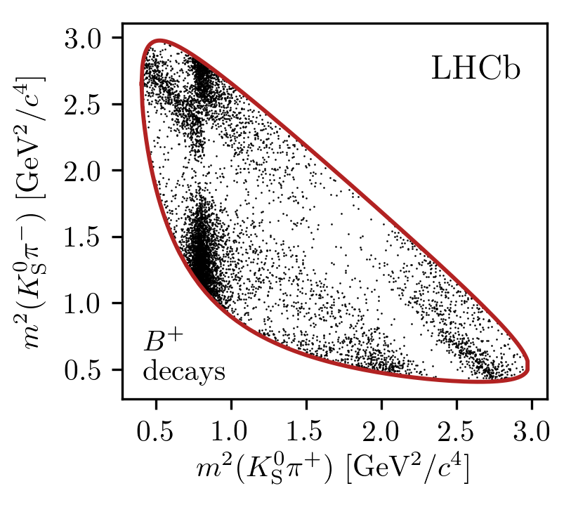
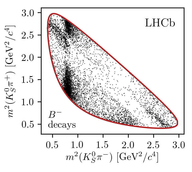
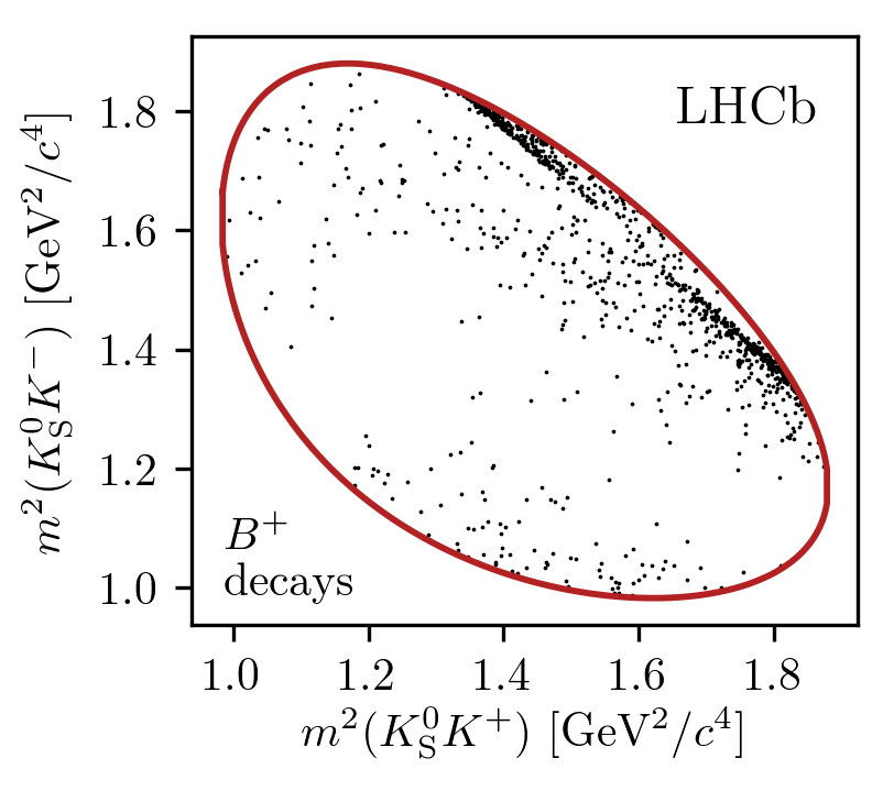
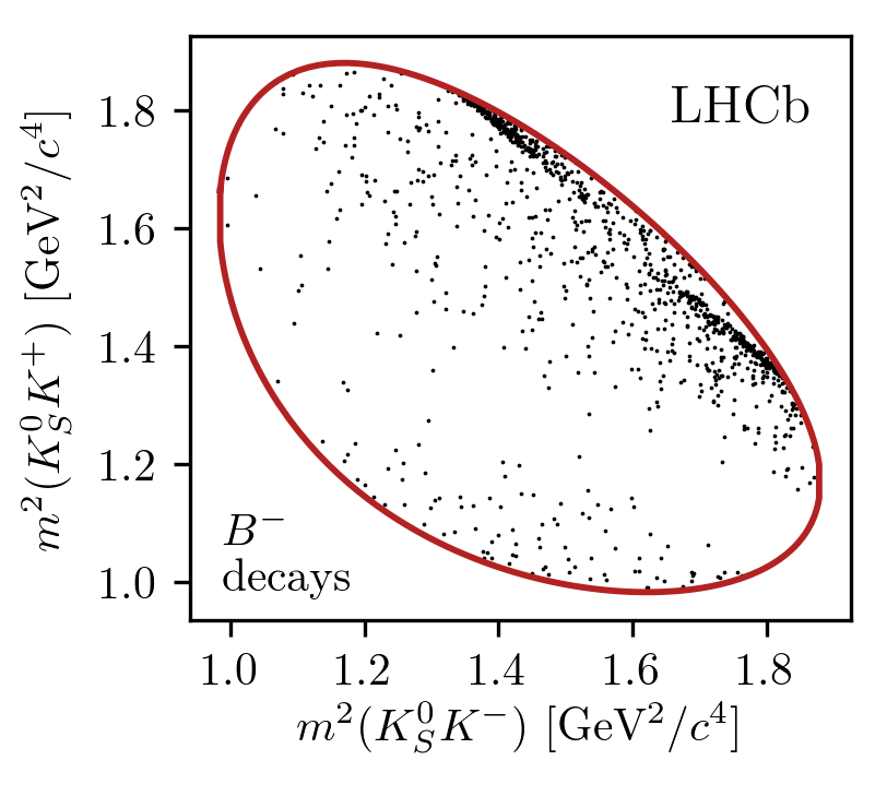
Figure 2: Dalitz plot for ${D}$ decays of (left) ${{{B}^{+}}}\rightarrow{D}{{K}^{+}}$ and (right) ${{{B}^{-}}}\rightarrow{D}{{K}^{-}}$ candidates in the signal region, in the (top) $D\rightarrow{{K}^{0}_{\mathrm{S}}}{{\pi}^{+}}{{\pi}^{-}}$ and (bottom) $D\rightarrow{{K}^{0}_{\mathrm{S}}}{{K}^{+}}{{K}^{-}}$ channels. The horizontal and vertical axes are interchanged between the ${{B}^{+}}$ and ${{B}^{-}}$ decay plots to aid visualisation of the $C\!P$ asymmetries between the two distributions.

5 The $DK$ and ${D}\pi$ invariant-mass spectra

The analysis uses a two-stage strategy to determine the $C\!P$ observables. First, an extended maximum-likelihood fit to the invariant-mass spectrum of all selected ${B}^{\pm}$ candidates in the mass range 5080 to 5800 $\text{\,Me\kern-1.00006ptV\!/}c^{2}$ is performed, with no partition of the $D$ phase space. This fit is referred to as the global fit. The global fit is used to determine the signal and background component parameterisations, which are subsequently used in a second stage where the data are split by $B$ charge and partitioned into the Dalitz plot bins to determine the $C\!P$ observables.

The invariant mass distributions of the selected ${B}^{\pm}$ candidates are shown for ${D}\rightarrow{{K}^{0}_{\mathrm{S}}}{{\pi}^{+}}{{\pi}^{-}}$ and ${D}\rightarrow{{K}^{0}_{\mathrm{S}}}{{K}^{+}}{{K}^{-}}$ candidates in Figs. 3 and 4, respectively, together with the results of the global fit superimposed. The invariant mass is kinematically constrained through a fit imposed on the full ${B}^{\pm}$ decay chain [63]. The $D$ and ${K}^{0}_{\mathrm{S}}$ candidates are constrained to their known masses[60] and the ${B}^{\pm}$ candidate momentum vector is required to point towards the associated PV. The data sample is split into 8 categories depending on the reconstructed $B$ decay, $D$ decay mode, and ${K}^{0}_{\mathrm{S}}$ category, since the latter exhibits slightly different mass resolutions. The fit is performed simultaneously for all categories in order to allow parameters to be shared.

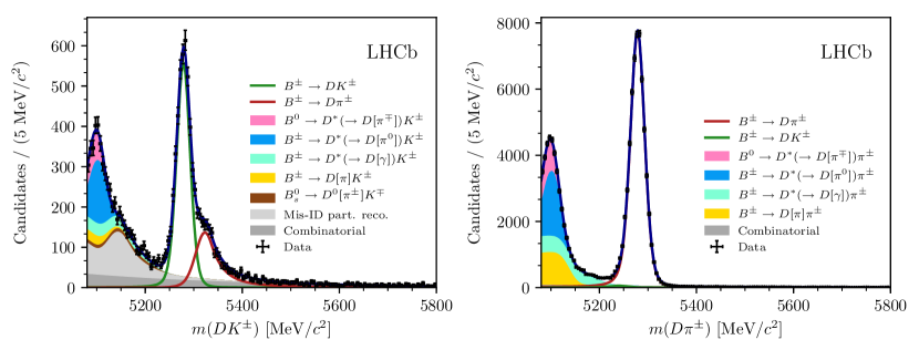
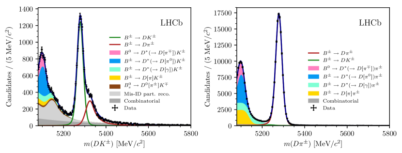
Figure 3: Invariant mass distributions for the (left) ${{{B}^{\pm}}\rightarrow{D}{{K}^{\pm}}}$ channel and (right) ${{{B}^{\pm}}\rightarrow{D}{{\pi}^{\pm}}}$ channel with ${D}\rightarrow{{K}^{0}_{\mathrm{S}}}{{\pi}^{+}}{{\pi}^{-}}$. The top (bottom) plots show data where the ${K}^{0}_{\mathrm{S}}$ candidate is long (downstream). Square brackets in the legend denote a particle that has not been reconstructed.

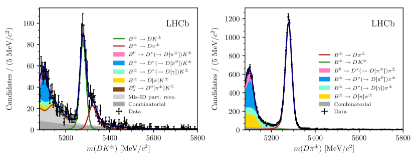
Figure 4: Invariant mass distributions for the (left) ${{{B}^{\pm}}\rightarrow{D}{{K}^{\pm}}}$ channel and (right) ${{{B}^{\pm}}\rightarrow{D}{{\pi}^{\pm}}}$ channel with ${D}\rightarrow{{K}^{0}_{\mathrm{S}}}{{K}^{+}}{{K}^{-}}$. The top (bottom) plots show data where the ${K}^{0}_{\mathrm{S}}$ candidate is long (downstream). Square brackets in the legend denote a particle that has not been reconstructed.

The peaks centered around 5280$\text{\,Me\kern-1.00006ptV\!/}c^{2}$ correspond to the signal ${{{B}^{\pm}}\rightarrow{D}{{K}^{\pm}}}$ and ${{{B}^{\pm}}\rightarrow{D}{{\pi}^{\pm}}}$ candidates. The parameterisation for the signal invariant-mass shape is determined from simulation; the invariant-mass distribution is modelled with a sum of the probability density function (PDF) for a Gaussian distribution, $f_{G}(m|m_{B},\sigma)$, and a modified Gaussian PDF that is used to account for the radiative tail and the wider resolution of signal events that are poorly reconstructed. The modified Gaussian has the form

$$f_{\mathrm{MG}}(m|m_{B},\sigma,\alpha_{L},\alpha_{R},\beta)\propto\left\{\begin{array}[]{ll}\exp\left[\frac{-\Delta m^{2}(1+\beta\Delta m^{2})}{2\sigma^{2}+\alpha_{L}\Delta m^{2}}\right],&\Delta m=m-m_{B}<0\\[8.0pt] \exp\left[\frac{-\Delta m^{2}(1+\beta\Delta m^{2})}{2\sigma^{2}+\alpha_{R}\Delta m^{2}}\right],&\Delta m=m-m_{B}>0,\end{array}\right.,$$ (10)

which is Gaussian when $\Delta m^{2}\ll\sigma^{2}/\alpha_{L/R}$ or $\Delta m^{2}\gg\beta^{-1}$ (with widths of $\sigma$ and $\sqrt{\alpha_{L/R}/\beta}$, respectively), with an exponential-like transition that is able to model the effect of the experimental resolution of LHCb. Thus, the signal PDF has the form

$$f_{\mathrm{signal}}(m|m_{B},\sigma,\alpha_{L},\alpha_{R},\beta,k)=k\cdot f_{\mathrm{MG}}(m|m_{B},\sigma,\alpha_{L},\alpha_{R},\beta)$$

$$+(1-k)\cdot f_{\mathrm{G}}(m|m_{B},\sigma)$$ (11)

The values of the tail parameters ($\alpha_{L}$, $\alpha_{R}$, $\beta$) and $k$ are fixed from simulation and are common for the two $D$ decays (which is possible due to the applied kinematic constraints) but different for each $B$ decay and type of ${K}^{0}_{\mathrm{S}}$ candidate. The signal mass, $m_{B}$, is determined in data and is the same for all categories. The width, $\sigma$, of the signal PDF is determined by the data and allowed to be different for each $B$ decay and type of ${K}^{0}_{\mathrm{S}}$ candidate. The width is narrower in ${{{B}^{\pm}}\rightarrow{D}{{K}^{\pm}}}$ decays compared to ${{{B}^{\pm}}\rightarrow{D}{{\pi}^{\pm}}}$ decays due to the smaller free energy in the decay. The width is approximately 3% narrower in decays with long ${K}^{0}_{\mathrm{S}}$ candidates. The signal yield is determined in each of the categories where the candidates are reconstructed as ${{{B}^{\pm}}\rightarrow{D}{{\pi}^{\pm}}}$. The signal yield in the corresponding category where the candidates are reconstructed as ${{{B}^{\pm}}\rightarrow{D}{{K}^{\pm}}}$ is determined by multiplying the ${{{B}^{\pm}}\rightarrow{D}{{\pi}^{\pm}}}$ yield by the parameters $\mathcal{B}\times\epsilon$. The parameter $\mathcal{B}$ corresponds to the ratio of the branching fractions for ${{{B}^{\pm}}\rightarrow{D}{{K}^{\pm}}}$ and ${{{B}^{\pm}}\rightarrow{D}{{\pi}^{\pm}}}$ decays, while the correction factor, $\epsilon$, takes into account the ratio of PID and selection efficiencies, and is determined for each pair of ${{{B}^{\pm}}\rightarrow{D}{{K}^{\pm}}}$ and ${{{B}^{\pm}}\rightarrow{D}{{\pi}^{\pm}}}$ categories and fixed in the fit. The parameter $\mathcal{B}$ is shared across all categories and is found to be consistent with Ref. [60].

To the right of the ${{{B}^{\pm}}\rightarrow{D}{{K}^{\pm}}}$ peak there is a visible contribution from ${{{B}^{\pm}}\rightarrow{D}{{\pi}^{\pm}}}$ decays that are reconstructed as ${{{B}^{\pm}}\rightarrow{D}{{K}^{\pm}}}$ decays. The corresponding contribution in the ${{{B}^{\pm}}\rightarrow{D}{{\pi}^{\pm}}}$ category is minimal due to the smaller branching fraction of ${{{B}^{\pm}}\rightarrow{D}{{K}^{\pm}}}$, but is accounted for in the fit. The rates of these cross-feed backgrounds are fixed from PID efficiencies determined in calibration data, which is reweighted to match the momentum and pseudorapidity distributions of the companion track of the signal. A data-driven approach is used to determine the PDF of ${{{B}^{\pm}}\rightarrow{D}{{\pi}^{\pm}}}$ decays that are reconstructed as ${{{B}^{\pm}}\rightarrow{D}{{K}^{\pm}}}$ candidates, by using ${{{B}^{\pm}}\rightarrow{D}{{\pi}^{\pm}}}$ decays and recalculating the invariant mass when the Kaon hypothesis is applied to the companion particle. Full details of the procedure are described in Ref. [10]. The same procedure is implemented to determine the PDF of ${{{B}^{\pm}}\rightarrow{D}{{K}^{\pm}}}$ decays reconstructed as ${{{B}^{\pm}}\rightarrow{D}{{\pi}^{\pm}}}$ candidates.

The background observed at invariant masses smaller than the signal peak are candidates that originate from other $B$-meson decays where not all decay products have been reconstructed. Due to the selected invariant-mass range it is only necessary to consider $B$ meson decays where a single photon or pion has not been reconstructed. This background type is split into three sources; the first where the candidate originates from a ${B}^{\pm}$ or ${B}^{0}$ meson, referred to as partially reconstructed background, the second where the candidate originates from a ${B}^{0}_{s}$ meson, and the third where the candidate originates from a ${B}^{\pm}$ or ${B}^{0}$ and furthermore one of the reconstructed tracks is assigned the kaon hypothesis, when the true particle is a pion. The latter type of background appears in the ${{{B}^{\pm}}\rightarrow{D}{{K}^{\pm}}}$ candidates and is referred to as misidentified partially reconstructed background. The corresponding type of background is not modelled in the ${{{B}^{\pm}}\rightarrow{D}{{\pi}^{\pm}}}$ candidates, since it is suppressed due to the branching fractions involved and the majority is removed by the lower invariant-mass requirement.

There are contributions from ${{B}^{0}}\rightarrow D^{*\pm}h^{\mp}$ and ${{B}^{\pm}}\rightarrow{D}^{*0}h^{\pm}$ decays in all categories, where the pion or the photon originating from the ${D}^{*}$ meson is not reconstructed. The invariant-mass distributions of these decays depend on the spin and mass of the missing particle as described in Ref. [24]. The parameters of these shapes are determined from simulation, with the exception of a free parameter in the fit to characterise the resolution. The decays ${B}^{\pm,0}\rightarrow{D}{{\pi}^{\pm}}\pi^{0,\mp}$ contribute to the ${{{B}^{\pm}}\rightarrow{D}{{\pi}^{\pm}}}$ candidates where one of the pions from the $B$ decay is not reconstructed. The shape of this background is determined from simulated ${{B}^{\pm}}\rightarrow{D}\rho^{\pm}$ and ${{B}^{0}}\rightarrow D\rho^{0}$ decays. The decays ${{B}^{\pm}}\rightarrow{D}{{K}^{\pm}}{{\pi}^{0}}$ and ${{B}^{0}}\rightarrow{D}{{K}^{+}}{{\pi}^{-}}$ contribute to the ${{{B}^{\pm}}\rightarrow{D}{{K}^{\pm}}}$ candidates where the pion is not reconstructed. The invariant-mass distribution for these events is based on the amplitude model of ${{B}^{0}}\rightarrow{D}{{K}^{+}}{{\pi}^{-}}$ decays [64]. The model is used to generate four-vectors of the decay products, which are smeared to account for the LHCb detector resolution. The invariant mass is then calculated omitting the particle that is not reconstructed, and this distribution is subsequently fit to determine the fixed distribution for the fit. The same shape is used for the ${{B}^{\pm}}\rightarrow{D}{{K}^{\pm}}{{\pi}^{0}}$ decay as the corresponding amplitude model is not available. Finally, the ${{{B}^{\pm}}\rightarrow{D}{{K}^{\pm}}}$ candidates also have a contribution from ${{B}^{0}_{s}}\rightarrow{{\kern 1.79993pt\overline{\kern-1.79993ptD}}{}^{0}}{{\pi}^{+}}{{K}^{-}}$ decays where the pion is not reconstructed. The shape of this contribution is determined in a similar manner to that of ${{B}^{0}}\rightarrow{D}{{K}^{+}}{{\pi}^{-}}$ decays using the ${{B}^{0}_{s}}\rightarrow{{\kern 1.79993pt\overline{\kern-1.79993ptD}}{}^{0}}{{\pi}^{+}}{{K}^{-}}$ amplitude model determined in Ref.[65].

The yield of the partially reconstructed background is a free parameter in each ${{{B}^{\pm}}\rightarrow{D}{{\pi}^{\pm}}}$ sample and related to the yield in the corresponding ${{{B}^{\pm}}\rightarrow{D}{{K}^{\pm}}}$ sample via the free parameter $\mathcal{B_{L}}$ and correction factors from PID and selection efficiencies. Analogously to the signal-yield parameterisation, $\mathcal{B_{L}}$ is a single parameter, common to all categories, but in this case has no direct physical meaning. The relative yield of ${{B}^{\pm}}\rightarrow D^{*}(\rightarrow{D}[\gamma]){{\pi}^{\pm}}$ and ${{B}^{0}}\rightarrow D^{*}(\rightarrow{D}[{{\pi}^{\mp}}]){{\pi}^{\pm}}$ decays, where the particle within the square brackets is the one not reconstructed, are fixed from branching fractions [60], and selection efficiencies determined from simulation. The fractional yields of ${{B}^{\pm}}\rightarrow D^{*0}(\rightarrow{D}[\gamma]){{\pi}^{\pm}}$, and ${B}^{\pm,0}\rightarrow D[\pi^{0,\mp}]{{\pi}^{\pm}}$ decays are determined in the fit and are constrained to be the same for each ${{{B}^{\pm}}\rightarrow{D}{{\pi}^{\pm}}}$ sample. Due to the lower yields in the ${{{B}^{\pm}}\rightarrow{D}{{K}^{\pm}}}$ category and presence of additional backgrounds, the relative fractions of the various ${B}^{\pm}$ and ${B}^{0}$ components are all fixed using information from branching fractions [60] and selection efficiencies from simulation. The yield of the ${{B}^{0}_{s}}\rightarrow{{\kern 1.79993pt\overline{\kern-1.79993ptD}}{}^{0}}{{\pi}^{+}}{{K}^{-}}$ decays is fixed relative to the yield of ${{{B}^{\pm}}\rightarrow{D}{{\pi}^{\pm}}}$ decays in the corresponding category using branching fractions [60], the fragmentation fraction [66], and relative selection efficiencies. Hence in total there are six free parameters to determine the partially reconstructed background yields. Four of these measure the yield in each ${{{B}^{\pm}}\rightarrow{D}{{\pi}^{\pm}}}$ sample and a further single parameter determines the yield in the corresponding ${{{B}^{\pm}}\rightarrow{D}{{K}^{\pm}}}$ sample. A final floating parameter determines the relative yield between two of the background components.

The shapes for the misidentified partially reconstructed backgrounds are determined from simulation, weighted by the PID efficiencies from calibration data. The yield of these backgrounds are determined from the partially reconstructed yields in the ${{{B}^{\pm}}\rightarrow{D}{{\pi}^{\pm}}}$ candidates, and the relative selection efficiencies, which include the PID efficiencies from calibration data and the selection efficiency due to requiring the reconstructed invariant mass to be above 5080$\text{\,Me\kern-1.00006ptV\!/}c^{2}$. The final component of background is combinatorial which is parameterised by an exponential function. The yield and slope of this background in each category are free parameters. The yields of the different signals and background types are integrated in the signal region 5249–5309$\text{\,Me\kern-1.00006ptV\!/}c^{2}$ and reported in Table 1. The ${{{B}^{\pm}}\rightarrow{D}{{K}^{\pm}}}$ yields in categories of different $D$ decay and type of ${K}^{0}_{\mathrm{S}}$ candidate have uncertainties that are smaller than their Poisson uncertainty since they are determined using the value of $\mathcal{B}$, which is measured from all ${{{B}^{\pm}}\rightarrow{D}{{K}^{\pm}}}$ candidates.

Table 1: The signal and background yields in the region $m_{B}\in[5249,5309]\text{\,Me\kern-1.00006ptV\!/}c^{2}$ as obtained in the fit. For the ${{{B}^{\pm}}\rightarrow{D}{{K}^{\pm}}}$ candidates, the yield of the partially reconstructed background includes the contributions from ${B}^{0}_{s}$ decays and misidentified partially reconstructed backgrounds.

	Reconstructed as:	${{{B}^{\pm}}\rightarrow{D}{{K}^{\pm}}}$		${{{B}^{\pm}}\rightarrow{D}{{\pi}^{\pm}}}$
$D$ decay	Component	long	downstream	long	downstream
$D\rightarrow{{K}^{0}_{\mathrm{S}}}{{\pi}^{+}}{{\pi}^{-}}$	${{B}^{\pm}}\rightarrow{D}{{K}^{\pm}}$	$3798\pm 41$	$8735\pm 89$	$182\pm 3$	$433\pm 8$
	${{B}^{\pm}}\rightarrow{D}{{\pi}^{\pm}}$	$342\pm 3$	$691\pm 5$	$55096\pm 240$	$124786\pm 368\phantom{1}$
	Part. reco. background	$114\pm 3$	$246\pm 6$	$\phantom{1}36\pm 7$	$\phantom{11}81\pm 12$
	Combinatorial	$\phantom{1}206\pm 36$	$\phantom{1}458\pm 60$	$\phantom{1}392\pm 66$	$\phantom{1}1142\pm 127$
${D}\rightarrow{{K}^{0}_{\mathrm{S}}}{{K}^{+}}{{K}^{-}}$	${{B}^{\pm}}\rightarrow{D}{{K}^{\pm}}$	$576\pm 8$	$1203\pm 15$	$\phantom{1}29\pm 1$	$\phantom{1}61\pm 1$
	${{B}^{\pm}}\rightarrow{D}{{\pi}^{\pm}}$	$\phantom{1}56\pm 1$	$104\pm 2$	$8196\pm 92$	$17863\pm 137$
	Part. reco background	$\phantom{1}17\pm 2$	$\phantom{1}34\pm 2$	$\phantom{11}5\pm 3$	$\phantom{1}11\pm 5$
	Combinatorial	$\phantom{11}44\pm 13$	$\phantom{11}75\pm 20$	$\phantom{1}127\pm 32$	$\phantom{1}288\pm 52$

6 ${C\!P}$ observables

To determine the $C\!P$ observables the data are divided into 16 categories ($B$ decay, $B$ charge, $D$ decay, type of ${K}^{0}_{\mathrm{S}}$ candidate) and then further split into each Dalitz plot bin. A simultaneous fit to the invariant-mass distribution is performed in all categories and Dalitz plot bins. The mass shape parameters are all fixed from the global mass fit. The lower limit of the invariant mass is increased to 5150$\text{\,Me\kern-1.00006ptV\!/}c^{2}$ to remove a large fraction of the partially reconstructed background. The signal yield in each bin is parameterised using Eq. (5) or the analogous set of expressions for ${{{B}^{\pm}}\rightarrow{D}{{\pi}^{\pm}}}$. These equations are normalised such that the parameters $h_{{{B}^{\pm}}}$ represent the total observed signal yield in each category, and these are measured independently. The yield of misidentified ${{{B}^{\pm}}\rightarrow{D}{{\pi}^{\pm}}}$ (${{{B}^{\pm}}\rightarrow{D}{{K}^{\pm}}}$) decays in each ${{{B}^{\pm}}\rightarrow{D}{{K}^{\pm}}}$ (${{{B}^{\pm}}\rightarrow{D}{{\pi}^{\pm}}}$) sample is determined by the PID efficiencies and the signal yield in the corresponding ${{{B}^{\pm}}\rightarrow{D}{{\pi}^{\pm}}}$ (${{{B}^{\pm}}\rightarrow{D}{{K}^{\pm}}}$) sample.

The parameters $x_{\pm}^{{D}{K}}$, $y_{\pm}^{{D}{K}}$, $x_{\xi}^{{D}\pi}$, and $y_{\xi}^{{D}\pi}$ are free parameters in the fit and common to the ${K}^{0}_{\mathrm{S}}$ and $D$ decay categories. The parameters $c_{i}$ and $s_{i}$ are fixed to those determined from the combination of BESIII and CLEO data  in Ref.[29] for the ${D}\rightarrow{{K}^{0}_{\mathrm{S}}}{{\pi}^{+}}{{\pi}^{-}}$ decays and in Ref. [30] for the ${D}\rightarrow{{K}^{0}_{\mathrm{S}}}{{K}^{+}}{{K}^{-}}$ decays. The $F_{i}$ parameters for each $D$ decay are determined in the fit; separate sets of $F_{i}$ parameters are determined for the two types of ${K}^{0}_{\mathrm{S}}$ candidates because the efficiency profile over the Dalitz plot differs between the ${K}^{0}_{\mathrm{S}}$ selections. Since the $F_{i}$ parameters must satisfy the constraints $\sum_{i}F_{i}=1,\,F_{i}\in[0,1]$, the fit can suffer from instability if they are included in a naive way due to large correlations. Therefore, the $F_{i}$ parameters are reparameterised as a series of recursive fractions with parameters, $\mathcal{R}_{i}$, determined in the fit. The relation between the $F_{i}$ and $\mathcal{R}_{i}$ parameters is given by

$$F_{i}=\left\{\begin{array}[]{ll}\mathcal{R}_{i}&,\quad i=-\mathcal{N}\\ \mathcal{R}_{i}\prod_{j<i}(1-\mathcal{R}_{j})&,\quad-\mathcal{N}<i<+\mathcal{N}\\ \phantom{R_{i}}\prod_{j<i}(1-\mathcal{R}_{j})&,\quad i=+\mathcal{N}.\end{array}\right.,$$ (15)

for a binning scheme with $2\times\mathcal{N}$ bins.

The yield of the combinatorial background in each bin is a free parameter. The yield of the partially reconstructed background from ${B}^{\pm}$ or ${B}^{0}$ decays in the ${{{B}^{\pm}}\rightarrow{D}{{\pi}^{\pm}}}$ and ${{{B}^{\pm}}\rightarrow{D}{{K}^{\pm}}}$ samples is also a free parameter in each bin. The composition of the partially reconstructed background is determined from the global fit described in Sect. 5, taking into account the change in the lower limit of invariant mass. The yield of the misidentified partially reconstructed background in the ${{{B}^{\pm}}\rightarrow{D}{{K}^{\pm}}}$ samples is determined via the background yield in the corresponding ${{{B}^{\pm}}\rightarrow{D}{{\pi}^{\pm}}}$ bin and the relative PID and selection efficiencies. The yield of the ${{B}^{0}_{s}}\rightarrow{{\kern 1.79993pt\overline{\kern-1.79993ptD}}{}^{0}}{{K}^{-}}{{\pi}^{+}}$ background is fixed from the global fit and is divided into the Dalitz plot bins according to the $F_{i}$ such that it has the distribution of a ${D}^{0}$ decay in the $B^{+}$ categories and the distribution of a ${\kern 1.79993pt\overline{\kern-1.79993ptD}}{}^{0}$ decay in the $B^{-}$ categories.

There is a small fraction of bins where either the partially reconstructed background or combinatoric background yield is less than one. These bins are identified in a preliminary fit and the background yield is fixed to zero. This procedure is carried out to improve the fit stability.

Pseudoexperiments are performed to investigate any potential biases or remaining instabilities in the fit. The candidate yields and mass distributions in these pseudoexperiments are based on the global fit results. The pull distributions are well described by a Gaussian function and are found to have mean and width consistent with 0 and 1, respectively.

The results for $x_{\pm}^{{D}{K}}$, $y_{\pm}^{{D}{K}}$, $x_{\xi}^{{D}\pi}$, and $y_{\xi}^{{D}\pi}$ are presented in Fig. 5 along with their likelihood contours, where only statistical uncertainties are considered. The two vectors defined by the origin and the end-point coordinates $(x_{-}^{{D}{K}},y_{-}^{{D}{K}})$ and $(x_{+}^{{D}{K}},y_{+}^{{D}{K}})$ give the values for $r_{B}^{{D}{K}}$ for ${{B}^{-}}$ and ${{B}^{+}}$ decays. The signature for $C\!P$ violation is that these vectors must have non-zero length and have a non-zero opening angle between them, since this angle is equal to $2\gamma$, as illustrated on the figure. Therefore, the data exhibit unambiguous features of $C\!P$ violation as expected. The relation between the hadronic parameters in ${{{B}^{\pm}}\rightarrow{D}{{\pi}^{\pm}}}$ and ${{{B}^{\pm}}\rightarrow{D}{{K}^{\pm}}}$ decays is also illustrated in Fig 5, where the vector defined by the coordinates ($x_{\xi}^{{D}\pi}$,$y_{\xi}^{{D}\pi}$) is the relative magnitude of $r_{B}$ between the two decay modes. It is consistent with the expectation of 5%  [41]. The normalization constants give global asymmetries that are consistent with the expectation of asymmetries from production, detection and neutral kaon effects.

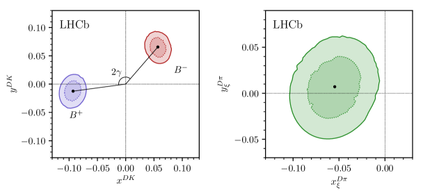
Figure 5: Confidence levels at 68.2 % and 95.5 % probability for (left, blue) $(x_{+}^{{D}{{K}^{\pm}}},y_{+}^{{D}{{K}^{\pm}}})$, (left, red) $(x_{-}^{{D}{{K}^{\pm}}},y_{-}^{{D}{{K}^{\pm}}})$, and (right, green) $(x_{\xi}^{{D}{{\pi}^{\pm}}},y_{\xi}^{{D}{{\pi}^{\pm}}})$ as measured in ${{{B}^{\pm}}\rightarrow{D}{{K}^{\pm}}}$ and ${{{B}^{\pm}}\rightarrow{D}{{\pi}^{\pm}}}$ decays with a profile likelihood scan. The black dots show the central values

A series of cross checks is carried out by performing separate fits by splitting the data sample into data-taking periods by year, type of ${K}^{0}_{\mathrm{S}}$ candidate, $D$-decay, hardware trigger path, and magnet polarity. The results are consistent between the datasets. As an additional cross check, the two-stage fit procedure is repeated with a number of different selections applied to the data. Of particular interest are the alternative selections that significantly affect the presence of specific backgrounds: the fits where the value of the BDT threshold is varied to decrease the level of combinatorial background and those where the choice of PID selection is changed to result in a substantially lower level of misidentified ${{{B}^{\pm}}\rightarrow{D}{{\pi}^{\pm}}}$ decays and misidentified partially reconstructed background in the ${{{B}^{\pm}}\rightarrow{D}{{K}^{\pm}}}$ candidates. The variations in the central values for the $C\!P$ observables are consistent within the statistical uncertainty associated with the change in the data sample.

In order to assess the goodness of fit and to demonstrate that the equations involving the $C\!P$ parameters provide a good description of the signal yields in data, an alternative fit is performed where the signal yield in each ${{{B}^{\pm}}\rightarrow{D}{{K}^{\pm}}}$ and ${{{B}^{\pm}}\rightarrow{D}{{\pi}^{\pm}}}$ bin is measured independently. The alternate fit is performed simultaneously in all categories in order to correctly determine the yield of misidentified candidates. These yields are compared with those predicted from the values of $(x_{\pm}^{{D}{K}},y_{\pm}^{{D}{K}})$ in the default fit and a high level of agreement is found. In order to visualise the observed $C\!P$ violation, the asymmetry, $(N^{-}_{-i}-N^{+}_{+i})/(N^{-}_{-i}+N^{+}_{+i})$, is computed for effective bin pairs, defined to comprise bin $i$ for a ${{B}^{+}}$ decay and bin $-i$ for a ${{B}^{-}}$ decay. Figure 6 shows the obtained asymmetries and those predicted by the values of the $C\!P$ observables obtained in the fit. A further fit that does not allow for $C\!P$ violation is carried out by imposing the conditions $x_{+}^{{D}{K}}$ = $x_{-}^{{D}{K}}$, $y_{+}^{{D}{K}}$ = $y_{-}^{{D}{K}}$. This determines the predicted asymmetry arising from detector and production effects. In the ${{{B}^{\pm}}\rightarrow{D}{{K}^{\pm}}}$ sample the $C\!P$ violation is clearly visible as the data are inconsistent with the $C\!P$-conserved hypothesis. The observed asymmetries correspond to a $\sim 10\sigma$ deviation given the expectation in the $C\!P$-conserving scenario. The predicted asymmetries in the ${{{B}^{\pm}}\rightarrow{D}{{\pi}^{\pm}}}$ decay are an order of magnitude smaller. The data in this analysis cannot distinguish between the $C\!P$-violating and $C\!P$-conserving predictions for ${{{B}^{\pm}}\rightarrow{D}{{\pi}^{\pm}}}$ due to the relatively large statistical uncertainties.

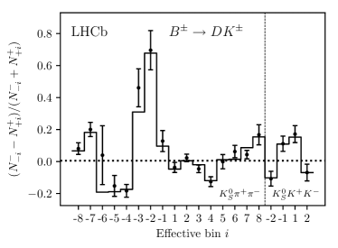
Figure 6: The bin-by-bin asymmetries $(N^{-}_{-i}-N^{+}_{+i})/(N^{-}_{-i}+N^{+}_{+i})$ for each Dalitz-plot bin number for (left) ${{{B}^{\pm}}\rightarrow{D}{{K}^{\pm}}}$ decays and (right) ${{{B}^{\pm}}\rightarrow{D}{{\pi}^{\pm}}}$ decays. The prediction from the central values of the $C\!P$-violation observables is shown with a solid line and the asymmetries obtained in fits with independent bin yields are shown with the error bars. The predicted asymmetries in a fit that does not allow for $C\!P$ violation are shown with a dotted line. The vertical dashed line separates the ${{K}^{0}_{\mathrm{S}}}{{\pi}^{+}}{{\pi}^{-}}$ and ${{K}^{0}_{\mathrm{S}}}{{K}^{+}}{{K}^{-}}$ bins on the horizontal axis.

7 Systematic uncertainties

Table 2: Overview of all sources of uncertainty, $\sigma$, on $x_{\pm}^{{D}{K}}$, $y_{\pm}^{{D}{K}}$, $x_{\xi}^{{D}\pi}$, and $y_{\xi}^{{D}\pi}$. All uncertainties are quoted $\times 10^{-2}$.

Source	$\sigma(x_{-}^{{D}{K}})$	$\sigma(y_{-}^{{D}{K}})$	$\sigma(x_{+}^{{D}{K}})$	$\sigma(y_{+}^{{D}{K}})$	$\sigma(x_{\xi}^{{D}\pi})$	$\sigma(y_{\xi}^{{D}\pi})$
Statistical	0.96	1.14	0.98	1.23	1.99	2.33
Strong-phase inputs	0.23	0.35	0.18	0.28	0.14	0.18
Efficiency correction of $(c_{i},s_{i})$	0.11	0.05	0.05	0.10	0.08	0.09
Mass-shape parameters	0.05	0.08	0.03	0.08	0.16	0.17
PID efficiencies	0.03	0.03	0.01	0.05	0.02	0.02
Fixed yield ratios	0.05	0.06	0.03	0.06	0.02	0.02
Mass-shape bin dependence	0.05	0.07	0.04	0.08	0.07	0.09
Part. reco. physics effects	0.04	0.10	0.15	0.05	0.10	0.09
Small backgrounds	0.11	0.16	0.13	0.12	0.08	0.13
Dalitz-bin migration	0.04	0.08	0.08	0.11	0.18	0.10
$C\!P$ violation of ${K}^{0}_{\mathrm{S}}$	0.03	0.04	0.08	0.08	0.09	0.46
$D$ mixing	0.04	0.01	0.00	0.02	0.02	0.01
Bias correction	0.04	0.03	0.02	0.04	0.09	0.05
Total LHCb-related uncertainty	0.20	0.25	0.24	0.26	0.32	0.54
Total systematic uncertainty	0.31	0.43	0.30	0.38	0.35	0.57

Systematic uncertainties on the measurements of the $C\!P$ observables are evaluated and are presented in Table 2. The limited precision on ($c_{i}$, $s_{i}$) coming from the combined BESIII and CLEO [29, 30] results induces uncertainties on the $C\!P$ parameters. These uncertainties are evaluated by fitting the data multiple times, each time with different ($c_{i}$, $s_{i}$) values sampled according to their experimental uncertainties and correlations. The resulting standard deviation of each distribution of the $C\!P$ observables is assigned as the systematic uncertainty. The size of the systematic uncertainty is notably much smaller than the corresponding uncertainty in Ref. [10] due to the improvement in the knowledge of these strong-phase parameters [29, 30].

The non-uniform efficiency profile over the Dalitz plot means that the values of ($c_{i}$,$s_{i}$) appropriate for this analysis can differ from those measured in Refs. [29, 30], which correspond to the case where there is no variation in efficiency over the Dalitz plot. Amplitude models from Refs. [67, 46] are used to calculate the values of $c_{i}$ and $s_{i}$ both with and without the efficiency profiles determined from simulation. The shift in the $c_{i}$ and $s_{i}$ values is taken as an estimate of the size of this effect. Pseudoexperiments are generated assuming the shifted $c_{i}$ and $s_{i}$ values and fit with the default values of $c_{i}$ and $s_{i}$. The mean bias of each $C\!P$ observable is assigned as a systematic uncertainty. The assumption that the relative variation of efficiency over the Dalitz plot is the same in selected ${{{B}^{\pm}}\rightarrow{D}{{K}^{\pm}}}$ and ${{{B}^{\pm}}\rightarrow{D}{{\pi}^{\pm}}}$ candidates is verified in simulated samples of similar size to the ${{{B}^{\pm}}\rightarrow{D}{{\pi}^{\pm}}}$ yields observed in data. No statistically significant difference is observed and no systematic uncertainty is assigned.

The uncertainties from the fixed invariant-mass shapes determined in the global fit are propagated to the $C\!P$ observables through a resampling method [68]. The following procedure, which takes into account the fact that some parameters are determined in simulation and others in data, is carried out a hundred times. First, the simulated decays that were used to determine the nominal mass shape parameters are each resampled with replacement and fit to determine an alternative set of parameters. Then, the final dataset is resampled with replacement and the global fit is repeated using the alternative fixed shape parameters, to determine alternative values for the parameters that are determined from real data. Finally, the $C\!P$ fit is performed using the alternative invariant-mass parameterisations, without resampling the final dataset. The standard deviation of the $C\!P$ observables obtained via this procedure is taken as the systematic uncertainty due to the fixed parameterisation.

The PID efficiencies are varied within their uncertainties in the global and $C\!P$ fit and the standard deviation of the $C\!P$ parameters is taken as the systematic uncertainty. A similar method is used to determine the uncertainties due to the fixed fractions between different partially reconstructed backgrounds where the uncertainties on the fixed fractions are those from the branching fractions [60] and the selection efficiencies.

The $C\!P$ fit assumes the same mass shape for each component in each Dalitz plot bin. For the signal and cross-feed backgrounds the shapes are redetermined in each bin using the same procedures described in Sect. 5. The variance is very small due to weak correlations between phase-space coordinates and particle kinematics. The combinatorial slope can also vary from bin to bin, as the relative rate of combinatorial background with and without a real ${D}^{0}$ meson will not be constant. The size of this effect is determined through the study of the high invariant-mass sideband where only combinatorial background contributes. Pseudodata are generated where this variation in mass shape across the Dalitz plot bins is replicated for signal, cross-feed and combinatorial backgrounds, and the generated samples are fit with the default fit assumptions of the same shape in each bin. The mean bias is assigned as the systematic uncertainty.

The partially reconstructed background shape is also expected to vary in each bin, however the leading source of this effect is due to the individual components of this background having a different distribution over the Dalitz plot. Some partially reconstructed backgrounds will be distributed as ${D}^{0}$ (${\kern 1.79993pt\overline{\kern-1.79993ptD}}{}^{0}$) $\rightarrow$ ${D}\rightarrow{{K}^{0}_{\mathrm{S}}}{h}^{+}{h}^{-}$ for reconstructed ${{B}^{-}}$ (${{B}^{+}}$) candidates, while others will be distributed as a ${{D}^{0}}$–${{\kern 1.79993pt\overline{\kern-1.79993ptD}}{}^{0}}$ admixture depending on the relevant $C\!P$-violation parameters. Pseudodata are generated, where the $D$-decay phase-space distributions for ${{B}^{\pm}}\rightarrow{D}^{*}K^{\pm}$ and ${{B}^{\pm}}\rightarrow{D}K^{*+}$ background events are based on the $C\!P$ parameters reported in Ref. [69]. No $C\!P$ violation is introduced into the partially reconstructed background in the ${{{B}^{\pm}}\rightarrow{D}{{\pi}^{\pm}}}$ samples since it is expected to be small, and the ${{B}^{0}}\rightarrow{D}\rho^{0}$ background is treated as an equal mix of ${D}^{0}$ and ${\kern 1.79993pt\overline{\kern-1.79993ptD}}{}^{0}$ since either pion can be reconstructed. The generated pseudodata are fitted with the default fit and the mean bias is assigned as the systematic uncertainty.

Systematic uncertainties are assigned for small residual backgrounds that contaminate the data sample but are not accounted for in the fit. Their impact is assessed by generating pseudoexperiments that contain these backgrounds and are fit with the default model. The mean bias is assigned as the uncertainty. One source of background is from ${{\mathchar 28931\relax}^{0}_{b}}\rightarrow{D}p{{\pi}^{-}}$ decays where the pion is not reconstructed and the proton is misidentified as a kaon. This background is modelled as a ${\kern 1.79993pt\overline{\kern-1.79993ptD}}{}^{0}$-like contribution in ${{B}^{-}}$ decays, and has an expected yield of 0.5% of the ${{{B}^{\pm}}\rightarrow{D}{{K}^{\pm}}}$ signal. A further, even smaller, background is ${{\mathchar 28931\relax}^{0}_{b}}\rightarrow{{\mathchar 28931\relax}^{+}_{c}}(\rightarrow p{{K}^{0}_{\mathrm{S}}}{{\pi}^{+}}{{\pi}^{-}}){{\pi}^{-}}$ decays where the ${\pi}^{+}$ meson in the $\Lambda_{c}^{+}$ decay is missed, and the $p$ reconstructed as the ${\pi}^{+}$ from the $D$-decay. The effective distribution of the reconstructed $D$ meson is unknown and is assigned to be ${\kern 1.79993pt\overline{\kern-1.79993ptD}}{}^{0}$-like in ${{B}^{-}}$ decays to be conservative. The mass shapes and rates of these backgrounds are determined from simulation. Another source of background comes from residual $B\rightarrow{D}\mu\nu$ decays, where the rate (less than 0.2 % relative to the signal mode, after the applied veto) and shape are determined from simulation with PID efficiencies from calibration data. The residual semileptonic ${D}$ decay background has a rate of less than 0.1% of signal and the distribution of these events on the Dalitz plot is determined through a simplified simulation [59] taking into account various $K^{*}$ mesons. Finally, a small peaking background from ${{B}^{\pm}}\rightarrow{D}(\rightarrow{{K}^{\pm}}{{\pi}^{\mp}}){{K}^{0}_{\mathrm{S}}}{{\pi}^{\pm}}$ decays where the kaon is reconstructed as the companion and the other particles are assigned to the $D$ decay is considered. The yield of this background is determined to be 0.5% of the signal yield in ${{{B}^{\pm}}\rightarrow{D}{{K}^{\pm}}}$ by a data driven study of the invariant-mass distribution of switched tracks. The distribution on the Dalitz plot is determined through the simplified simulation [59] where different $K^{*\pm}\rightarrow{{K}^{0}_{\mathrm{S}}}{{\pi}^{\pm}}$ resonances are generated.

The main effect of migration from one Dalitz plot bin to another is implicitly taken into account by using the data to determine the $F_{i}$, which thus include the effects of the net bin migration. However, a small effect arises because of the differences in the distributions of the ${{{B}^{\pm}}\rightarrow{D}{{K}^{\pm}}}$ and ${{{B}^{\pm}}\rightarrow{D}{{\pi}^{\pm}}}$ decays due to the differing hadronic decay parameters. To investigate this, data points are generated according to the amplitude model in Ref. [67] with $C\!P$ observables consistent with expectation [69, 5]. To smear these data points on the Dalitz plot, an event is selected from full LHCb simulation and the difference in $m^{2}_{+}$ and $m^{2}_{-}$ between its true and reconstructed quantities is applied to the data point in order to determine its reconstructed bin. The difference between true and reconstructed quantities is multiplied by a factor of 1.2 to account for differences in resolution between data and simulation. Pseudoexperiments are generated based on the expected reconstructed yields in each bin and fit with a nominal fit where the $c_{i}$ and $s_{i}$ parameters are determined by the amplitude model [67]. The mean bias in the $C\!P$ violation parameters is taken as the systematic uncertainty, which is small.

The impact of ignoring the $C\!P$ violation and matter effects in ${K}^{0}_{\mathrm{S}}$ decays is determined through generating pseudoexperiments taking into account all these effects as detailed in Ref. [39], where LHCb simulation is used to obtain the ${K}^{0}_{\mathrm{S}}$ lifetime acceptance and momentum distribution. The size of the bias found is consistent with those expected from Ref. [39], where it was also predicted that the relative uncertainties on ${{{B}^{\pm}}\rightarrow{D}{{\pi}^{\pm}}}$ observables are be expected to be larger than for ${{{B}^{\pm}}\rightarrow{D}{{K}^{\pm}}}$ observables. This is found to be true, but even the most significant uncertainty, on $y_{\xi}^{{D}\pi}$, is an order of magnitude smaller than the corresponding statistical uncertainty. The effect of ignoring charm mixing is expected to be minimal, given that the first-order effects are inherently taken into account when the $F_{i}$ parameters are measured as a part of the fit [38]. This is verified by generating pseudoexperiments that include charm mixing and fitting them with the nominal fit.

In previous studies, a bias correction has been necessary when similar measurements have been performed with lower signal yields [10] leading to some fit instabilities. In this case, the higher yields have resulted in a bias that is of negligible size and hence no correction is applied. Nonetheless, the uncertainty on the biases are assigned as the systematic uncertainties.

In general, all the systematic uncertainties are small in comparison to the statistical uncertainties. There is no dominant source of systematic uncertainty for all $C\!P$ observables, however the description of backgrounds, either those not modelled or the modelling of the partially reconstructed backgrounds are some of the larger sources. The uncertainty attributed to the precision of the strong-phase measurements is of similar size to the total LHCb-related systematic uncertainty.

8 Interpretation

The $C\!P$ observables are measured to be

$$\begin{split}x_{-}^{DK}&=(\phantom{-}5.68\pm 0.96\pm 0.20\pm 0.23)\times 10^{-2},\\ y_{-}^{DK}&=(\phantom{-}6.55\pm 1.14\pm 0.25\pm 0.35)\times 10^{-2},\\ x_{+}^{DK}&=(-9.30\pm 0.98\pm 0.24\pm 0.18)\times 10^{-2},\\ y_{+}^{DK}&=(-1.25\pm 1.23\pm 0.26\pm 0.28)\times 10^{-2},\\ x_{\xi}^{D\pi}&=(-5.47\pm 1.99\pm 0.32\pm 0.14)\times 10^{-2},\\ y_{\xi}^{D\pi}&=(\phantom{-}0.71\pm 2.33\pm 0.54\pm 0.18)\times 10^{-2},\end{split}$$ (16)

where the first uncertainty is statistical, the second arises from systematic effects in the method or detector considerations, and the third from external inputs of strong-phase measurements from the combination of CLEO and BESIII [29, 27] results. The correlation matrices for each source of uncertainty are available in the appendices in Tables 3-5.

The $C\!P$ observables are interpreted in terms of the underlying physics parameters $\gamma$, and $r_{B}$ and $\delta_{B}$ for each ${B}^{\pm}$ decay mode. The interpretation is done via a maximum likelihood fit using a frequentist treatment as described in Ref. [44]. The solution for the physics parameters has a two-fold ambiguity as the equations are invariant under the simultaneous substitutions $\gamma\rightarrow\gamma+180^{\circ}$ and $\delta_{B}\rightarrow\delta_{B}+180^{\circ}$. The solution that satisfies $0<\gamma<180^{\circ}$ is chosen, and leads to

$$\begin{split}\gamma&=(68.7^{+5.2}_{-5.1})^{\circ},\\ r_{B}^{{{D}{{K}^{\pm}}}}&=0.0904^{+0.0077}_{-0.0075},\\ \delta_{B}^{{{D}{{K}^{\pm}}}}&=(118.3^{+5.5}_{-5.6})^{\circ},\\ r_{B}^{D\pi^{\pm}}&=0.0050\pm 0.0017,\\ \delta_{B}^{D\pi^{\pm}}&=(291^{+24}_{-26})^{\circ}.\end{split}$$ (17)

Pseudoexperiments are carried out to confirm that the value of $\gamma$ is extracted without bias. This is the most precise single measurement of $\gamma$ to date. The result is consistent with the indirect determination $\gamma=\left(65.66^{+0.90}_{-2.65}\right)^{\circ}$ [6]. The confidence limits for $\gamma$ are illustrated in Fig. 7, while Fig. 8 shows the two-dimensional confidence regions obtained for the ($\gamma$, $r_{B}$) and ($r_{B}$, $\delta_{B}$) parameter combinations. The results for $\gamma$, $r_{B}^{{D}{K}}$ ,and $\delta_{B}^{{D}{K}}$ are consistent with their current world averages [5, 6] which include the LHCb results obtained with the 2011–2016 data. The knowledge of $r_{B}^{{D}\pi}$ and $\delta_{B}^{{D}\pi}$ from other sources is limited, with the combination of many observables presented in Ref. [44] providing two possible solutions. The results here have a single solution, and favour a central value that is consistent with the expectation for $r_{B}^{{D}\pi}$, given the value of $r_{B}^{{D}{K}}$ and CKM elements [41]. This is likely to remove the two-solution aspect in future combinations of $\gamma$ and associated hadronic parameters. The low value of $r_{B}^{{D}\pi}$ means that the direct contribution to $\gamma$ from ${{{B}^{\pm}}\rightarrow{D}{{\pi}^{\pm}}}$ decays in this measurement is minimal. However the ability to use this decay mode to determine the efficiency has approximately halved the total LHCb related experimental systematic uncertainty in comparison to Ref. [10]. The new inputs from the BESIII collaboration have led to the strong-phase related uncertainty on $\gamma$ to be approximately 1^∘, which is a significant reduction compared to the propagated uncertainty when only CLEO measurements were available.

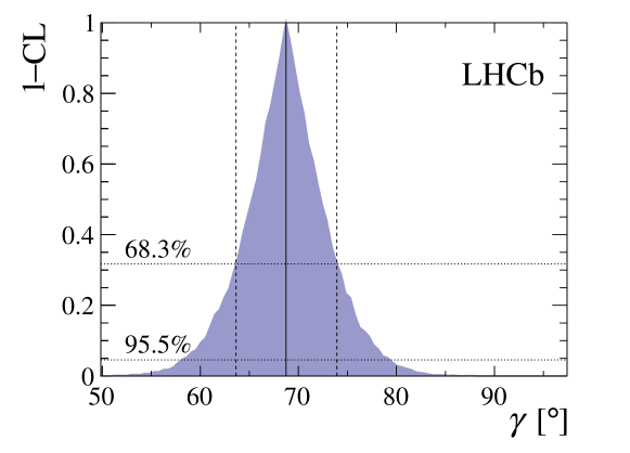
Figure 7: Confidence limits for the CKM angle $\gamma$ obtained using the method described in Ref. [44].

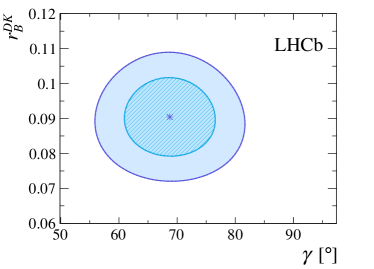
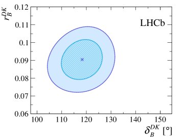
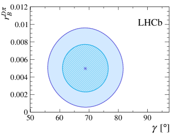
Figure 8: The 68 % and 95 % confidence regions for combinations of the physics parameters $(\gamma,r_{B}^{{D}{K}},\delta_{B}^{{D}{K}},r_{B}^{{D}\pi},\delta_{B}^{{D}\pi})$ obtained using the methods described in Ref. [44].

9 Conclusions

In summary, the decays ${{{B}^{\pm}}\rightarrow{D}{{K}^{\pm}}}$ and ${{{B}^{\pm}}\rightarrow{D}{{\pi}^{\pm}}}$ with ${D}\rightarrow{{K}^{0}_{\mathrm{S}}}{{\pi}^{+}}{{\pi}^{-}}$ or ${D\rightarrow{{K}^{0}_{\mathrm{S}}}{{K}^{+}}{{K}^{-}}}$ obtained from the full LHCb dataset collected to date, corresponding to an integrated luminosity of 9 $\text{\,fb}^{-1}$, have been analysed to determine the CKM angle $\gamma$. The sensitivity to $\gamma$ comes almost entirely from ${{{B}^{\pm}}\rightarrow{D}{{K}^{\pm}}}$ decays where the signal yields of reconstructed events are approximately 13600 (1900) in the ${D}\rightarrow{{K}^{0}_{\mathrm{S}}}{{\pi}^{+}}{{\pi}^{-}}$ (${D}\rightarrow{{K}^{0}_{\mathrm{S}}}{{K}^{+}}{{K}^{-}}$) decay modes. The ${{{B}^{\pm}}\rightarrow{D}{{\pi}^{\pm}}}$ data is primarily used to control effects due to selection and reconstruction of the data, which leads to small experimental systematic uncertainties. The analysis is performed in bins of the $D$-decay Dalitz plot and a combination of measurements performed by the CLEO and BESIII collaborations presented in Refs. [29, 30] are used to provide input on the $D$-decay strong-phase parameters ($c_{i}$,$s_{i}$). Such an approach allows the analysis to be free from model-dependent assumptions on the strong-phase variation across the Dalitz plot. The analysis also determines the hadronic parameters $r_{B}$ and $\delta_{B}$ for each ${B}^{\pm}$ decay mode. Those of the ${{{B}^{\pm}}\rightarrow{D}{{K}^{\pm}}}$ decay are consistent with current averages, and those of the ${{{B}^{\pm}}\rightarrow{D}{{\pi}^{\pm}}}$ decay are obtained with the best precision to date, and have not previously been measured using these $D$-decay modes. The CKM angle $\gamma$ is determined to be $\gamma=(68.7^{+5.2}_{-5.1})^{\circ}$, where the result is limited by statistical uncertainties. This is the most precise measurement of $\gamma$ from a single analysis, and supersedes the results in Refs. [10, 31].

Appendices

Appendix A Correlation matrices

The correlations matrices for the measured observables are shown in Tables 3–5 for the statistical uncertainties, the experimental systematic uncertainties, and the strong-phase-related uncertainties, respectively.

Table 3: Statistical uncertainties, $\sigma$, and correlation matrix for $x_{\pm}^{{D}{K}}$, $y_{\pm}^{{D}{K}}$, $x_{\xi}^{{D}\pi}$, and $y_{\xi}^{{D}\pi}$.

Uncertainty $(\times 10^{-2})$
	$x_{-}^{{D}{K}}$	$y_{-}^{{D}{K}}$	$x_{+}^{{D}{K}}$	$y_{+}^{{D}{K}}$	$x_{\xi}^{{D}\pi}$	$y_{\xi}^{{D}\pi}$
$\sigma$	$0.96$	$1.14$	$0.98$	$1.23$	$1.99$	$2.33$
Correlation matrix
	$x_{-}^{{D}{K}}$	$y_{-}^{{D}{K}}$	$x_{+}^{{D}{K}}$	$y_{+}^{{D}{K}}$	$x_{\xi}^{{D}\pi}$	$y_{\xi}^{{D}\pi}$
$x_{-}^{{D}{K}}$	$\phantom{-}1\phantom{.000}$	$-0.125$	$-0.013$	$\phantom{-}0.019$	$\phantom{-}0.037$	$-0.161$
$y_{-}^{{D}{K}}$		$\phantom{-}1\phantom{.000}$	$-0.011$	$-0.010$	$\phantom{-}0.097$	$\phantom{-}0.041$
$x_{+}^{{D}{K}}$			$\phantom{-}1\phantom{.000}$	$\phantom{-}0.105$	$-0.108$	$\phantom{-}0.032$
$y_{+}^{{D}{K}}$				$\phantom{-}1\phantom{.000}$	$-0.070$	$-0.147$
$x_{\xi}^{{D}\pi}$					$\phantom{-}1\phantom{.000}$	$\phantom{-}0.150$
$y_{\xi}^{{D}\pi}$						$\phantom{-}1\phantom{.000}$

Table 4: Total LHCb-related systematic uncertainties, $\sigma$, for $x_{\pm}^{{D}{K}}$, $y_{\pm}^{{D}{K}}$, $x_{\xi}^{{D}\pi}$, and $y_{\xi}^{{D}\pi}$, and the corresponding correlation matrix.

Uncertainty $(\times 10^{-2})$
	$x_{-}^{{D}{K}}$	$y_{-}^{{D}{K}}$	$x_{+}^{{D}{K}}$	$y_{+}^{{D}{K}}$	$x_{\xi}^{{D}\pi}$	$y_{\xi}^{{D}\pi}$
$\sigma$	$0.20$	$0.25$	$0.24$	$0.26$	$0.32$	$0.54$
Correlation matrix
	$x_{-}^{{D}{K}}$	$y_{-}^{{D}{K}}$	$x_{+}^{{D}{K}}$	$y_{+}^{{D}{K}}$	$x_{\xi}^{{D}\pi}$	$y_{\xi}^{{D}\pi}$
$x_{-}^{{D}{K}}$	$\phantom{-}1\phantom{.000}$	$\phantom{-}0.864$	$\phantom{-}0.734$	$\phantom{-}0.897$	$\phantom{-}0.349$	$\phantom{-}0.318$
$y_{-}^{{D}{K}}$		$\phantom{-}1\phantom{.000}$	$\phantom{-}0.874$	$\phantom{-}0.903$	$\phantom{-}0.408$	$\phantom{-}0.362$
$x_{+}^{{D}{K}}$			$\phantom{-}1\phantom{.000}$	$\phantom{-}0.771$	$\phantom{-}0.563$	$\phantom{-}0.447$
$y_{+}^{{D}{K}}$				$\phantom{-}1\phantom{.000}$	$\phantom{-}0.507$	$\phantom{-}0.451$
$x_{\xi}^{{D}\pi}$					$\phantom{-}1\phantom{.000}$	$\phantom{-}0.484$
$y_{\xi}^{{D}\pi}$						$\phantom{-}1\phantom{.000}$

Table 5: Systematic uncertainties, $\sigma$, for $x_{\pm}^{{D}{K}}$, $y_{\pm}^{{D}{K}}$, $x_{\xi}^{{D}\pi}$, and $y_{\xi}^{{D}\pi}$ due to strong-phase inputs, the corresponding correlation matrix.

Uncertainty $(\times 10^{-2})$
	$x_{-}^{{D}{K}}$	$y_{-}^{{D}{K}}$	$x_{+}^{{D}{K}}$	$y_{+}^{{D}{K}}$	$x_{\xi}^{{D}\pi}$	$y_{\xi}^{{D}\pi}$
$\sigma$	$0.23$	$0.35$	$0.18$	$0.28$	$0.14$	$0.18$
Correlation matrix
	$x_{-}^{{D}{K}}$	$y_{-}^{{D}{K}}$	$x_{+}^{{D}{K}}$	$y_{+}^{{D}{K}}$	$x_{\xi}^{{D}\pi}$	$y_{\xi}^{{D}\pi}$
$x_{-}^{{D}{K}}$	$\phantom{-}1\phantom{.000}$	$-0.047$	$-0.490$	$\phantom{-}0.322$	$\phantom{-}0.189$	$\phantom{-}0.144$
$y_{-}^{{D}{K}}$		$\phantom{-}1\phantom{.000}$	$\phantom{-}0.059$	$-0.237$	$-0.116$	$-0.117$
$x_{+}^{{D}{K}}$			$\phantom{-}1\phantom{.000}$	$\phantom{-}0.061$	$\phantom{-}0.004$	$-0.139$
$y_{+}^{{D}{K}}$				$\phantom{-}1\phantom{.000}$	$\phantom{-}0.127$	$-0.199$
$x_{\xi}^{{D}\pi}$					$\phantom{-}1\phantom{.000}$	$\phantom{-}0.638$
$y_{\xi}^{{D}\pi}$						$\phantom{-}1\phantom{.000}$

LHCb collaboration

R. Aaij³¹, C. Abellán Beteta⁴⁹, T. Ackernley⁵⁹, B. Adeva⁴⁵, M. Adinolfi⁵³, H. Afsharnia⁹, C.A. Aidala⁸⁴, S. Aiola²⁵, Z. Ajaltouni⁹, S. Akar⁶⁴, J. Albrecht¹⁴, F. Alessio⁴⁷, M. Alexander⁵⁸, A. Alfonso Albero⁴⁴, Z. Aliouche⁶¹, G. Alkhazov³⁷, P. Alvarez Cartelle⁴⁷, S. Amato², Y. Amhis¹¹, L. An²¹, L. Anderlini²¹, A. Andreianov³⁷, M. Andreotti²⁰, F. Archilli¹⁶, A. Artamonov⁴³, M. Artuso⁶⁷, K. Arzymatov⁴¹, E. Aslanides¹⁰, M. Atzeni⁴⁹, B. Audurier¹¹, S. Bachmann¹⁶, M. Bachmayer⁴⁸, J.J. Back⁵⁵, S. Baker⁶⁰, P. Baladron Rodriguez⁴⁵, V. Balagura¹¹, W. Baldini²⁰, J. Baptista Leite¹, R.J. Barlow⁶¹, S. Barsuk¹¹, W. Barter⁶⁰, M. Bartolini^23,i, F. Baryshnikov⁸⁰, J.M. Basels¹³, G. Bassi²⁸, B. Batsukh⁶⁷, A. Battig¹⁴, A. Bay⁴⁸, M. Becker¹⁴, F. Bedeschi²⁸, I. Bediaga¹, A. Beiter⁶⁷, V. Belavin⁴¹, S. Belin²⁶, V. Bellee⁴⁸, K. Belous⁴³, I. Belov³⁹, I. Belyaev³⁸, G. Bencivenni²², E. Ben-Haim¹², A. Berezhnoy³⁹, R. Bernet⁴⁹, D. Berninghoff¹⁶, H.C. Bernstein⁶⁷, C. Bertella⁴⁷, E. Bertholet¹², A. Bertolin²⁷, C. Betancourt⁴⁹, F. Betti^19,e, M.O. Bettler⁵⁴, Ia. Bezshyiko⁴⁹, S. Bhasin⁵³, J. Bhom³³, L. Bian⁷², M.S. Bieker¹⁴, S. Bifani⁵², P. Billoir¹², M. Birch⁶⁰, F.C.R. Bishop⁵⁴, A. Bizzeti^21,s, M. Bjørn⁶², M.P. Blago⁴⁷, T. Blake⁵⁵, F. Blanc⁴⁸, S. Blusk⁶⁷, D. Bobulska⁵⁸, V. Bocci³⁰, J.A. Boelhauve¹⁴, O. Boente Garcia⁴⁵, T. Boettcher⁶³, A. Boldyrev⁸¹, A. Bondar^42,v, N. Bondar³⁷, S. Borghi⁶¹, M. Borisyak⁴¹, M. Borsato¹⁶, J.T. Borsuk³³, S.A. Bouchiba⁴⁸, T.J.V. Bowcock⁵⁹, A. Boyer⁴⁷, C. Bozzi²⁰, M.J. Bradley⁶⁰, S. Braun⁶⁵, A. Brea Rodriguez⁴⁵, M. Brodski⁴⁷, J. Brodzicka³³, A. Brossa Gonzalo⁵⁵, D. Brundu²⁶, A. Buonaura⁴⁹, C. Burr⁴⁷, A. Bursche²⁶, A. Butkevich⁴⁰, J.S. Butter³¹, J. Buytaert⁴⁷, W. Byczynski⁴⁷, S. Cadeddu²⁶, H. Cai⁷², R. Calabrese^20,g, L. Calefice¹⁴, L. Calero Diaz²², S. Cali²², R. Calladine⁵², M. Calvi^24,j, M. Calvo Gomez⁸³, P. Camargo Magalhaes⁵³, A. Camboni⁴⁴, P. Campana²², D.H. Campora Perez⁴⁷, A.F. Campoverde Quezada⁵, S. Capelli^24,j, L. Capriotti^19,e, A. Carbone^19,e, G. Carboni²⁹, R. Cardinale^23,i, A. Cardini²⁶, I. Carli⁶, P. Carniti^24,j, K. Carvalho Akiba³¹, A. Casais Vidal⁴⁵, G. Casse⁵⁹, M. Cattaneo⁴⁷, G. Cavallero⁴⁷, S. Celani⁴⁸, J. Cerasoli¹⁰, A.J. Chadwick⁵⁹, M.G. Chapman⁵³, M. Charles¹², Ph. Charpentier⁴⁷, G. Chatzikonstantinidis⁵², C.A. Chavez Barajas⁵⁹, M. Chefdeville⁸, C. Chen³, S. Chen²⁶, A. Chernov³³, S.-G. Chitic⁴⁷, V. Chobanova⁴⁵, S. Cholak⁴⁸, M. Chrzaszcz³³, A. Chubykin³⁷, V. Chulikov³⁷, P. Ciambrone²², M.F. Cicala⁵⁵, X. Cid Vidal⁴⁵, G. Ciezarek⁴⁷, P.E.L. Clarke⁵⁷, M. Clemencic⁴⁷, H.V. Cliff⁵⁴, J. Closier⁴⁷, J.L. Cobbledick⁶¹, V. Coco⁴⁷, J.A.B. Coelho¹¹, J. Cogan¹⁰, E. Cogneras⁹, L. Cojocariu³⁶, P. Collins⁴⁷, T. Colombo⁴⁷, L. Congedo¹⁸, A. Contu²⁶, N. Cooke⁵², G. Coombs⁵⁸, G. Corti⁴⁷, C.M. Costa Sobral⁵⁵, B. Couturier⁴⁷, D.C. Craik⁶³, J. Crkovská⁶⁶, M. Cruz Torres¹, R. Currie⁵⁷, C.L. Da Silva⁶⁶, E. Dall’Occo¹⁴, J. Dalseno⁴⁵, C. D’Ambrosio⁴⁷, A. Danilina³⁸, P. d’Argent⁴⁷, A. Davis⁶¹, O. De Aguiar Francisco⁶¹, K. De Bruyn⁷⁷, S. De Capua⁶¹, M. De Cian⁴⁸, J.M. De Miranda¹, L. De Paula², M. De Serio^18,d, D. De Simone⁴⁹, P. De Simone²², J.A. de Vries⁷⁸, C.T. Dean⁶⁶, W. Dean⁸⁴, D. Decamp⁸, L. Del Buono¹², B. Delaney⁵⁴, H.-P. Dembinski¹⁴, A. Dendek³⁴, V. Denysenko⁴⁹, D. Derkach⁸¹, O. Deschamps⁹, F. Desse¹¹, F. Dettori^26,f, B. Dey⁷², P. Di Nezza²², S. Didenko⁸⁰, L. Dieste Maronas⁴⁵, H. Dijkstra⁴⁷, V. Dobishuk⁵¹, A.M. Donohoe¹⁷, F. Dordei²⁶, M. Dorigo^28,w, A.C. dos Reis¹, L. Douglas⁵⁸, A. Dovbnya⁵⁰, A.G. Downes⁸, K. Dreimanis⁵⁹, M.W. Dudek³³, L. Dufour⁴⁷, V. Duk⁷⁶, P. Durante⁴⁷, J.M. Durham⁶⁶, D. Dutta⁶¹, M. Dziewiecki¹⁶, A. Dziurda³³, A. Dzyuba³⁷, S. Easo⁵⁶, U. Egede⁶⁸, V. Egorychev³⁸, S. Eidelman^42,v, S. Eisenhardt⁵⁷, S. Ek-In⁴⁸, L. Eklund⁵⁸, S. Ely⁶⁷, A. Ene³⁶, E. Epple⁶⁶, S. Escher¹³, J. Eschle⁴⁹, S. Esen³¹, T. Evans⁴⁷, A. Falabella¹⁹, J. Fan³, Y. Fan⁵, B. Fang⁷², N. Farley⁵², S. Farry⁵⁹, D. Fazzini^24,j, P. Fedin³⁸, M. Féo⁴⁷, P. Fernandez Declara⁴⁷, A. Fernandez Prieto⁴⁵, J.M. Fernandez-tenllado Arribas⁴⁴, F. Ferrari^19,e, L. Ferreira Lopes⁴⁸, F. Ferreira Rodrigues², S. Ferreres Sole³¹, M. Ferrillo⁴⁹, M. Ferro-Luzzi⁴⁷, S. Filippov⁴⁰, R.A. Fini¹⁸, M. Fiorini^20,g, M. Firlej³⁴, K.M. Fischer⁶², C. Fitzpatrick⁶¹, T. Fiutowski³⁴, F. Fleuret^11,b, M. Fontana⁴⁷, F. Fontanelli^23,i, R. Forty⁴⁷, V. Franco Lima⁵⁹, M. Franco Sevilla⁶⁵, M. Frank⁴⁷, E. Franzoso²⁰, G. Frau¹⁶, C. Frei⁴⁷, D.A. Friday⁵⁸, J. Fu²⁵, Q. Fuehring¹⁴, W. Funk⁴⁷, E. Gabriel³¹, T. Gaintseva⁴¹, A. Gallas Torreira⁴⁵, D. Galli^19,e, S. Gallorini²⁷, S. Gambetta⁵⁷, Y. Gan³, M. Gandelman², P. Gandini²⁵, Y. Gao⁴, M. Garau²⁶, L.M. Garcia Martin⁵⁵, P. Garcia Moreno⁴⁴, J. García Pardiñas⁴⁹, B. Garcia Plana⁴⁵, F.A. Garcia Rosales¹¹, L. Garrido⁴⁴, D. Gascon⁴⁴, C. Gaspar⁴⁷, R.E. Geertsema³¹, D. Gerick¹⁶, L.L. Gerken¹⁴, E. Gersabeck⁶¹, M. Gersabeck⁶¹, T. Gershon⁵⁵, D. Gerstel¹⁰, Ph. Ghez⁸, V. Gibson⁵⁴, M. Giovannetti^22,k, A. Gioventù⁴⁵, P. Gironella Gironell⁴⁴, L. Giubega³⁶, C. Giugliano^20,g, K. Gizdov⁵⁷, E.L. Gkougkousis⁴⁷, V.V. Gligorov¹², C. Göbel⁶⁹, E. Golobardes⁸³, D. Golubkov³⁸, A. Golutvin^60,80, A. Gomes^1,a, S. Gomez Fernandez⁴⁴, F. Goncalves Abrantes⁶⁹, M. Goncerz³³, G. Gong³, P. Gorbounov³⁸, I.V. Gorelov³⁹, C. Gotti^24,j, E. Govorkova³¹, J.P. Grabowski¹⁶, R. Graciani Diaz⁴⁴, T. Grammatico¹², L.A. Granado Cardoso⁴⁷, E. Graugés⁴⁴, E. Graverini⁴⁸, G. Graziani²¹, A. Grecu³⁶, L.M. Greeven³¹, P. Griffith²⁰, L. Grillo⁶¹, S. Gromov⁸⁰, L. Gruber⁴⁷, B.R. Gruberg Cazon⁶², C. Gu³, M. Guarise²⁰, P. A. Günther¹⁶, E. Gushchin⁴⁰, A. Guth¹³, Y. Guz^43,47, T. Gys⁴⁷, T. Hadavizadeh⁶⁸, G. Haefeli⁴⁸, C. Haen⁴⁷, J. Haimberger⁴⁷, S.C. Haines⁵⁴, T. Halewood-leagas⁵⁹, P.M. Hamilton⁶⁵, Q. Han⁷, X. Han¹⁶, T.H. Hancock⁶², S. Hansmann-Menzemer¹⁶, N. Harnew⁶², T. Harrison⁵⁹, C. Hasse⁴⁷, M. Hatch⁴⁷, J. He⁵, M. Hecker⁶⁰, K. Heijhoff³¹, K. Heinicke¹⁴, A.M. Hennequin⁴⁷, K. Hennessy⁵⁹, L. Henry^25,46, J. Heuel¹³, A. Hicheur², D. Hill⁶², M. Hilton⁶¹, S.E. Hollitt¹⁴, P.H. Hopchev⁴⁸, J. Hu¹⁶, J. Hu⁷¹, W. Hu⁷, W. Huang⁵, X. Huang⁷², W. Hulsbergen³¹, R.J. Hunter⁵⁵, M. Hushchyn⁸¹, D. Hutchcroft⁵⁹, D. Hynds³¹, P. Ibis¹⁴, M. Idzik³⁴, D. Ilin³⁷, P. Ilten⁵², A. Inglessi³⁷, A. Ishteev⁸⁰, K. Ivshin³⁷, R. Jacobsson⁴⁷, S. Jakobsen⁴⁷, E. Jans³¹, B.K. Jashal⁴⁶, A. Jawahery⁶⁵, V. Jevtic¹⁴, M. Jezabek³³, F. Jiang³, M. John⁶², D. Johnson⁴⁷, C.R. Jones⁵⁴, T.P. Jones⁵⁵, B. Jost⁴⁷, N. Jurik⁴⁷, S. Kandybei⁵⁰, Y. Kang³, M. Karacson⁴⁷, J.M. Kariuki⁵³, N. Kazeev⁸¹, M. Kecke¹⁶, F. Keizer^54,47, M. Kenzie⁵⁵, T. Ketel³², B. Khanji⁴⁷, A. Kharisova⁸², S. Kholodenko⁴³, K.E. Kim⁶⁷, T. Kirn¹³, V.S. Kirsebom⁴⁸, O. Kitouni⁶³, S. Klaver³¹, K. Klimaszewski³⁵, S. Koliiev⁵¹, A. Kondybayeva⁸⁰, A. Konoplyannikov³⁸, P. Kopciewicz³⁴, R. Kopecna¹⁶, P. Koppenburg³¹, M. Korolev³⁹, I. Kostiuk^31,51, O. Kot⁵¹, S. Kotriakhova^37,30, P. Kravchenko³⁷, L. Kravchuk⁴⁰, R.D. Krawczyk⁴⁷, M. Kreps⁵⁵, F. Kress⁶⁰, S. Kretzschmar¹³, P. Krokovny^42,v, W. Krupa³⁴, W. Krzemien³⁵, W. Kucewicz^33,l, M. Kucharczyk³³, V. Kudryavtsev^42,v, H.S. Kuindersma³¹, G.J. Kunde⁶⁶, T. Kvaratskheliya³⁸, D. Lacarrere⁴⁷, G. Lafferty⁶¹, A. Lai²⁶, A. Lampis²⁶, D. Lancierini⁴⁹, J.J. Lane⁶¹, R. Lane⁵³, G. Lanfranchi²², C. Langenbruch¹³, J. Langer¹⁴, O. Lantwin^49,80, T. Latham⁵⁵, F. Lazzari^28,t, R. Le Gac¹⁰, S.H. Lee⁸⁴, R. Lefèvre⁹, A. Leflat³⁹, S. Legotin⁸⁰, O. Leroy¹⁰, T. Lesiak³³, B. Leverington¹⁶, H. Li⁷¹, L. Li⁶², P. Li¹⁶, X. Li⁶⁶, Y. Li⁶, Y. Li⁶, Z. Li⁶⁷, X. Liang⁶⁷, T. Lin⁶⁰, R. Lindner⁴⁷, V. Lisovskyi¹⁴, R. Litvinov²⁶, G. Liu⁷¹, H. Liu⁵, S. Liu⁶, X. Liu³, A. Loi²⁶, J. Lomba Castro⁴⁵, I. Longstaff⁵⁸, J.H. Lopes², G. Loustau⁴⁹, G.H. Lovell⁵⁴, Y. Lu⁶, D. Lucchesi^27,m, S. Luchuk⁴⁰, M. Lucio Martinez³¹, V. Lukashenko³¹, Y. Luo³, A. Lupato⁶¹, E. Luppi^20,g, O. Lupton⁵⁵, A. Lusiani^28,r, X. Lyu⁵, L. Ma⁶, S. Maccolini^19,e, F. Machefert¹¹, F. Maciuc³⁶, V. Macko⁴⁸, P. Mackowiak¹⁴, S. Maddrell-Mander⁵³, O. Madejczyk³⁴, L.R. Madhan Mohan⁵³, O. Maev³⁷, A. Maevskiy⁸¹, D. Maisuzenko³⁷, M.W. Majewski³⁴, S. Malde⁶², B. Malecki⁴⁷, A. Malinin⁷⁹, T. Maltsev^42,v, H. Malygina¹⁶, G. Manca^26,f, G. Mancinelli¹⁰, R. Manera Escalero⁴⁴, D. Manuzzi^19,e, D. Marangotto^25,o, J. Maratas^9,u, J.F. Marchand⁸, U. Marconi¹⁹, S. Mariani^21,47,h, C. Marin Benito¹¹, M. Marinangeli⁴⁸, P. Marino⁴⁸, J. Marks¹⁶, P.J. Marshall⁵⁹, G. Martellotti³⁰, L. Martinazzoli^47,j, M. Martinelli^24,j, D. Martinez Santos⁴⁵, F. Martinez Vidal⁴⁶, A. Massafferri¹, M. Materok¹³, R. Matev⁴⁷, A. Mathad⁴⁹, Z. Mathe⁴⁷, V. Matiunin³⁸, C. Matteuzzi²⁴, K.R. Mattioli⁸⁴, A. Mauri³¹, E. Maurice^11,b, J. Mauricio⁴⁴, M. Mazurek³⁵, M. McCann⁶⁰, L. Mcconnell¹⁷, T.H. Mcgrath⁶¹, A. McNab⁶¹, R. McNulty¹⁷, J.V. Mead⁵⁹, B. Meadows⁶⁴, C. Meaux¹⁰, G. Meier¹⁴, N. Meinert⁷⁵, D. Melnychuk³⁵, S. Meloni^24,j, M. Merk^31,78, A. Merli²⁵, L. Meyer Garcia², M. Mikhasenko⁴⁷, D.A. Milanes⁷³, E. Millard⁵⁵, M. Milovanovic⁴⁷, M.-N. Minard⁸, L. Minzoni^20,g, S.E. Mitchell⁵⁷, B. Mitreska⁶¹, D.S. Mitzel⁴⁷, A. Mödden¹⁴, R.A. Mohammed⁶², R.D. Moise⁶⁰, T. Mombächer¹⁴, I.A. Monroy⁷³, S. Monteil⁹, M. Morandin²⁷, G. Morello²², M.J. Morello^28,r, J. Moron³⁴, A.B. Morris⁷⁴, A.G. Morris⁵⁵, R. Mountain⁶⁷, H. Mu³, F. Muheim⁵⁷, M. Mukherjee⁷, M. Mulder⁴⁷, D. Müller⁴⁷, K. Müller⁴⁹, C.H. Murphy⁶², D. Murray⁶¹, P. Muzzetto²⁶, P. Naik⁵³, T. Nakada⁴⁸, R. Nandakumar⁵⁶, T. Nanut⁴⁸, I. Nasteva², M. Needham⁵⁷, I. Neri^20,g, N. Neri^25,o, S. Neubert⁷⁴, N. Neufeld⁴⁷, R. Newcombe⁶⁰, T.D. Nguyen⁴⁸, C. Nguyen-Mau⁴⁸, E.M. Niel¹¹, S. Nieswand¹³, N. Nikitin³⁹, N.S. Nolte⁴⁷, C. Nunez⁸⁴, A. Oblakowska-Mucha³⁴, V. Obraztsov⁴³, D.P. O’Hanlon⁵³, R. Oldeman^26,f, C.J.G. Onderwater⁷⁷, A. Ossowska³³, J.M. Otalora Goicochea², T. Ovsiannikova³⁸, P. Owen⁴⁹, A. Oyanguren⁴⁶, B. Pagare⁵⁵, P.R. Pais⁴⁷, T. Pajero^28,47,r, A. Palano¹⁸, M. Palutan²², Y. Pan⁶¹, G. Panshin⁸², A. Papanestis⁵⁶, M. Pappagallo^18,d, L.L. Pappalardo^20,g, C. Pappenheimer⁶⁴, W. Parker⁶⁵, C. Parkes⁶¹, C.J. Parkinson⁴⁵, B. Passalacqua²⁰, G. Passaleva²¹, A. Pastore¹⁸, M. Patel⁶⁰, C. Patrignani^19,e, C.J. Pawley⁷⁸, A. Pearce⁴⁷, A. Pellegrino³¹, M. Pepe Altarelli⁴⁷, S. Perazzini¹⁹, D. Pereima³⁸, P. Perret⁹, K. Petridis⁵³, A. Petrolini^23,i, A. Petrov⁷⁹, S. Petrucci⁵⁷, M. Petruzzo²⁵, A. Philippov⁴¹, L. Pica²⁸, M. Piccini⁷⁶, B. Pietrzyk⁸, G. Pietrzyk⁴⁸, M. Pili⁶², D. Pinci³⁰, J. Pinzino⁴⁷, F. Pisani⁴⁷, A. Piucci¹⁶, Resmi  P.K¹⁰, V. Placinta³⁶, S. Playfer⁵⁷, J. Plews⁵², M. Plo Casasus⁴⁵, F. Polci¹², M. Poli Lener²², M. Poliakova⁶⁷, A. Poluektov¹⁰, N. Polukhina^80,c, I. Polyakov⁶⁷, E. Polycarpo², G.J. Pomery⁵³, S. Ponce⁴⁷, A. Popov⁴³, D. Popov^5,47, S. Popov⁴¹, S. Poslavskii⁴³, K. Prasanth³³, L. Promberger⁴⁷, C. Prouve⁴⁵, V. Pugatch⁵¹, A. Puig Navarro⁴⁹, H. Pullen⁶², G. Punzi^28,n, W. Qian⁵, J. Qin⁵, R. Quagliani¹², B. Quintana⁸, N.V. Raab¹⁷, R.I. Rabadan Trejo¹⁰, B. Rachwal³⁴, J.H. Rademacker⁵³, M. Rama²⁸, M. Ramos Pernas⁵⁵, M.S. Rangel², F. Ratnikov^41,81, G. Raven³², M. Reboud⁸, F. Redi⁴⁸, F. Reiss¹², C. Remon Alepuz⁴⁶, Z. Ren³, V. Renaudin⁶², R. Ribatti²⁸, S. Ricciardi⁵⁶, D.S. Richards⁵⁶, K. Rinnert⁵⁹, P. Robbe¹¹, A. Robert¹², G. Robertson⁵⁷, A.B. Rodrigues⁴⁸, E. Rodrigues⁵⁹, J.A. Rodriguez Lopez⁷³, A. Rollings⁶², P. Roloff⁴⁷, V. Romanovskiy⁴³, M. Romero Lamas⁴⁵, A. Romero Vidal⁴⁵, J.D. Roth⁸⁴, M. Rotondo²², M.S. Rudolph⁶⁷, T. Ruf⁴⁷, J. Ruiz Vidal⁴⁶, A. Ryzhikov⁸¹, J. Ryzka³⁴, J.J. Saborido Silva⁴⁵, N. Sagidova³⁷, N. Sahoo⁵⁵, B. Saitta^26,f, D. Sanchez Gonzalo⁴⁴, C. Sanchez Gras³¹, C. Sanchez Mayordomo⁴⁶, R. Santacesaria³⁰, C. Santamarina Rios⁴⁵, M. Santimaria²², E. Santovetti^29,k, D. Saranin⁸⁰, G. Sarpis⁶¹, M. Sarpis⁷⁴, A. Sarti³⁰, C. Satriano^30,q, A. Satta²⁹, M. Saur⁵, D. Savrina^38,39, H. Sazak⁹, L.G. Scantlebury Smead⁶², S. Schael¹³, M. Schellenberg¹⁴, M. Schiller⁵⁸, H. Schindler⁴⁷, M. Schmelling¹⁵, T. Schmelzer¹⁴, B. Schmidt⁴⁷, O. Schneider⁴⁸, A. Schopper⁴⁷, M. Schubiger³¹, S. Schulte⁴⁸, M.H. Schune¹¹, R. Schwemmer⁴⁷, B. Sciascia²², A. Sciubba³⁰, S. Sellam⁴⁵, A. Semennikov³⁸, M. Senghi Soares³², A. Sergi^52,47, N. Serra⁴⁹, J. Serrano¹⁰, L. Sestini²⁷, A. Seuthe¹⁴, P. Seyfert⁴⁷, D.M. Shangase⁸⁴, M. Shapkin⁴³, I. Shchemerov⁸⁰, L. Shchutska⁴⁸, T. Shears⁵⁹, L. Shekhtman^42,v, Z. Shen⁴, V. Shevchenko⁷⁹, E.B. Shields^24,j, E. Shmanin⁸⁰, J.D. Shupperd⁶⁷, B.G. Siddi²⁰, R. Silva Coutinho⁴⁹, G. Simi²⁷, S. Simone^18,d, I. Skiba^20,g, N. Skidmore⁷⁴, T. Skwarnicki⁶⁷, M.W. Slater⁵², J.C. Smallwood⁶², J.G. Smeaton⁵⁴, A. Smetkina³⁸, E. Smith¹³, M. Smith⁶⁰, A. Snoch³¹, M. Soares¹⁹, L. Soares Lavra⁹, M.D. Sokoloff⁶⁴, F.J.P. Soler⁵⁸, A. Solovev³⁷, I. Solovyev³⁷, F.L. Souza De Almeida², B. Souza De Paula², B. Spaan¹⁴, E. Spadaro Norella^25,o, P. Spradlin⁵⁸, F. Stagni⁴⁷, M. Stahl⁶⁴, S. Stahl⁴⁷, P. Stefko⁴⁸, O. Steinkamp^49,80, S. Stemmle¹⁶, O. Stenyakin⁴³, H. Stevens¹⁴, S. Stone⁶⁷, M.E. Stramaglia⁴⁸, M. Straticiuc³⁶, D. Strekalina⁸⁰, S. Strokov⁸², F. Suljik⁶², J. Sun²⁶, L. Sun⁷², Y. Sun⁶⁵, P. Svihra⁶¹, P.N. Swallow⁵², K. Swientek³⁴, A. Szabelski³⁵, T. Szumlak³⁴, M. Szymanski⁴⁷, S. Taneja⁶¹, Z. Tang³, T. Tekampe¹⁴, F. Teubert⁴⁷, E. Thomas⁴⁷, K.A. Thomson⁵⁹, M.J. Tilley⁶⁰, V. Tisserand⁹, S. T’Jampens⁸, M. Tobin⁶, S. Tolk⁴⁷, L. Tomassetti^20,g, D. Torres Machado¹, D.Y. Tou¹², M. Traill⁵⁸, M.T. Tran⁴⁸, E. Trifonova⁸⁰, C. Trippl⁴⁸, A. Tsaregorodtsev¹⁰, G. Tuci^28,n, A. Tully⁴⁸, N. Tuning³¹, A. Ukleja³⁵, D.J. Unverzagt¹⁶, A. Usachov³¹, A. Ustyuzhanin^41,81, U. Uwer¹⁶, A. Vagner⁸², V. Vagnoni¹⁹, A. Valassi⁴⁷, G. Valenti¹⁹, N. Valls Canudas⁴⁴, M. van Beuzekom³¹, H. Van Hecke⁶⁶, E. van Herwijnen⁸⁰, C.B. Van Hulse¹⁷, M. van Veghel⁷⁷, R. Vazquez Gomez⁴⁵, P. Vazquez Regueiro⁴⁵, C. Vázquez Sierra³¹, S. Vecchi²⁰, J.J. Velthuis⁵³, M. Veltri^21,p, A. Venkateswaran⁶⁷, M. Veronesi³¹, M. Vesterinen⁵⁵, D. Vieira⁶⁴, M. Vieites Diaz⁴⁸, H. Viemann⁷⁵, X. Vilasis-Cardona⁸³, E. Vilella Figueras⁵⁹, P. Vincent¹², G. Vitali²⁸, A. Vollhardt⁴⁹, D. Vom Bruch¹², A. Vorobyev³⁷, V. Vorobyev^42,v, N. Voropaev³⁷, R. Waldi⁷⁵, J. Walsh²⁸, C. Wang¹⁶, J. Wang³, J. Wang⁷², J. Wang⁴, J. Wang⁶, M. Wang³, R. Wang⁵³, Y. Wang⁷, Z. Wang⁴⁹, D.R. Ward⁵⁴, H.M. Wark⁵⁹, N.K. Watson⁵², S.G. Weber¹², D. Websdale⁶⁰, C. Weisser⁶³, B.D.C. Westhenry⁵³, D.J. White⁶¹, M. Whitehead⁵³, D. Wiedner¹⁴, G. Wilkinson⁶², M. Wilkinson⁶⁷, I. Williams⁵⁴, M. Williams^63,68, M.R.J. Williams⁵⁷, F.F. Wilson⁵⁶, W. Wislicki³⁵, M. Witek³³, L. Witola¹⁶, G. Wormser¹¹, S.A. Wotton⁵⁴, H. Wu⁶⁷, K. Wyllie⁴⁷, Z. Xiang⁵, D. Xiao⁷, Y. Xie⁷, H. Xing⁷¹, A. Xu⁴, J. Xu⁵, L. Xu³, M. Xu⁷, Q. Xu⁵, Z. Xu⁵, Z. Xu⁴, D. Yang³, Y. Yang⁵, Z. Yang³, Z. Yang⁶⁵, Y. Yao⁶⁷, L.E. Yeomans⁵⁹, H. Yin⁷, J. Yu⁷⁰, X. Yuan⁶⁷, O. Yushchenko⁴³, K.A. Zarebski⁵², M. Zavertyaev^15,c, M. Zdybal³³, O. Zenaiev⁴⁷, M. Zeng³, D. Zhang⁷, L. Zhang³, S. Zhang⁴, Y. Zhang⁴⁷, Y. Zhang⁶², A. Zhelezov¹⁶, Y. Zheng⁵, X. Zhou⁵, Y. Zhou⁵, X. Zhu³, V. Zhukov^13,39, J.B. Zonneveld⁵⁷, S. Zucchelli^19,e, D. Zuliani²⁷, G. Zunica⁶¹.

¹Centro Brasileiro de Pesquisas Físicas (CBPF), Rio de Janeiro, Brazil
²Universidade Federal do Rio de Janeiro (UFRJ), Rio de Janeiro, Brazil
³Center for High Energy Physics, Tsinghua University, Beijing, China
⁴School of Physics State Key Laboratory of Nuclear Physics and Technology, Peking University, Beijing, China
⁵University of Chinese Academy of Sciences, Beijing, China
⁶Institute Of High Energy Physics (IHEP), Beijing, China
⁷Institute of Particle Physics, Central China Normal University, Wuhan, Hubei, China
⁸Univ. Grenoble Alpes, Univ. Savoie Mont Blanc, CNRS, IN2P3-LAPP, Annecy, France
⁹Université Clermont Auvergne, CNRS/IN2P3, LPC, Clermont-Ferrand, France
¹⁰Aix Marseille Univ, CNRS/IN2P3, CPPM, Marseille, France
¹¹Ijclab, Orsay, France
¹²LPNHE, Sorbonne Université, Paris Diderot Sorbonne Paris Cité, CNRS/IN2P3, Paris, France
¹³I. Physikalisches Institut, RWTH Aachen University, Aachen, Germany
¹⁴Fakultät Physik, Technische Universität Dortmund, Dortmund, Germany
¹⁵Max-Planck-Institut für Kernphysik (MPIK), Heidelberg, Germany
¹⁶Physikalisches Institut, Ruprecht-Karls-Universität Heidelberg, Heidelberg, Germany
¹⁷School of Physics, University College Dublin, Dublin, Ireland
¹⁸INFN Sezione di Bari, Bari, Italy
¹⁹INFN Sezione di Bologna, Bologna, Italy
²⁰INFN Sezione di Ferrara, Ferrara, Italy
²¹INFN Sezione di Firenze, Firenze, Italy
²²INFN Laboratori Nazionali di Frascati, Frascati, Italy
²³INFN Sezione di Genova, Genova, Italy
²⁴INFN Sezione di Milano-Bicocca, Milano, Italy
²⁵INFN Sezione di Milano, Milano, Italy
²⁶INFN Sezione di Cagliari, Monserrato, Italy
²⁷Universita degli Studi di Padova, Universita e INFN, Padova, Padova, Italy
²⁸INFN Sezione di Pisa, Pisa, Italy
²⁹INFN Sezione di Roma Tor Vergata, Roma, Italy
³⁰INFN Sezione di Roma La Sapienza, Roma, Italy
³¹Nikhef National Institute for Subatomic Physics, Amsterdam, Netherlands
³²Nikhef National Institute for Subatomic Physics and VU University Amsterdam, Amsterdam, Netherlands
³³Henryk Niewodniczanski Institute of Nuclear Physics Polish Academy of Sciences, Kraków, Poland
³⁴AGH - University of Science and Technology, Faculty of Physics and Applied Computer Science, Kraków, Poland
³⁵National Center for Nuclear Research (NCBJ), Warsaw, Poland
³⁶Horia Hulubei National Institute of Physics and Nuclear Engineering, Bucharest-Magurele, Romania
³⁷Petersburg Nuclear Physics Institute NRC Kurchatov Institute (PNPI NRC KI), Gatchina, Russia
³⁸Institute of Theoretical and Experimental Physics NRC Kurchatov Institute (ITEP NRC KI), Moscow, Russia
³⁹Institute of Nuclear Physics, Moscow State University (SINP MSU), Moscow, Russia
⁴⁰Institute for Nuclear Research of the Russian Academy of Sciences (INR RAS), Moscow, Russia
⁴¹Yandex School of Data Analysis, Moscow, Russia
⁴²Budker Institute of Nuclear Physics (SB RAS), Novosibirsk, Russia
⁴³Institute for High Energy Physics NRC Kurchatov Institute (IHEP NRC KI), Protvino, Russia, Protvino, Russia
⁴⁴ICCUB, Universitat de Barcelona, Barcelona, Spain
⁴⁵Instituto Galego de Física de Altas Enerxías (IGFAE), Universidade de Santiago de Compostela, Santiago de Compostela, Spain
⁴⁶Instituto de Fisica Corpuscular, Centro Mixto Universidad de Valencia - CSIC, Valencia, Spain
⁴⁷European Organization for Nuclear Research (CERN), Geneva, Switzerland
⁴⁸Institute of Physics, Ecole Polytechnique Fédérale de Lausanne (EPFL), Lausanne, Switzerland
⁴⁹Physik-Institut, Universität Zürich, Zürich, Switzerland
⁵⁰NSC Kharkiv Institute of Physics and Technology (NSC KIPT), Kharkiv, Ukraine
⁵¹Institute for Nuclear Research of the National Academy of Sciences (KINR), Kyiv, Ukraine
⁵²University of Birmingham, Birmingham, United Kingdom
⁵³H.H. Wills Physics Laboratory, University of Bristol, Bristol, United Kingdom
⁵⁴Cavendish Laboratory, University of Cambridge, Cambridge, United Kingdom
⁵⁵Department of Physics, University of Warwick, Coventry, United Kingdom
⁵⁶STFC Rutherford Appleton Laboratory, Didcot, United Kingdom
⁵⁷School of Physics and Astronomy, University of Edinburgh, Edinburgh, United Kingdom
⁵⁸School of Physics and Astronomy, University of Glasgow, Glasgow, United Kingdom
⁵⁹Oliver Lodge Laboratory, University of Liverpool, Liverpool, United Kingdom
⁶⁰Imperial College London, London, United Kingdom
⁶¹Department of Physics and Astronomy, University of Manchester, Manchester, United Kingdom
⁶²Department of Physics, University of Oxford, Oxford, United Kingdom
⁶³Massachusetts Institute of Technology, Cambridge, MA, United States
⁶⁴University of Cincinnati, Cincinnati, OH, United States
⁶⁵University of Maryland, College Park, MD, United States
⁶⁶Los Alamos National Laboratory (LANL), Los Alamos, United States
⁶⁷Syracuse University, Syracuse, NY, United States
⁶⁸School of Physics and Astronomy, Monash University, Melbourne, Australia, associated to ^55
69Pontifícia Universidade Católica do Rio de Janeiro (PUC-Rio), Rio de Janeiro, Brazil, associated to ^2
70Physics and Micro Electronic College, Hunan University, Changsha City, China, associated to ^7
71Guangdong Provencial Key Laboratory of Nuclear Science, Institute of Quantum Matter, South China Normal University, Guangzhou, China, associated to ^3
72School of Physics and Technology, Wuhan University, Wuhan, China, associated to ^3
73Departamento de Fisica , Universidad Nacional de Colombia, Bogota, Colombia, associated to ^12
74Universität Bonn - Helmholtz-Institut für Strahlen und Kernphysik, Bonn, Germany, associated to ^16
75Institut für Physik, Universität Rostock, Rostock, Germany, associated to ^16
76INFN Sezione di Perugia, Perugia, Italy, associated to ^20
77Van Swinderen Institute, University of Groningen, Groningen, Netherlands, associated to ^31
78Universiteit Maastricht, Maastricht, Netherlands, associated to ^31
79National Research Centre Kurchatov Institute, Moscow, Russia, associated to ^38
80National University of Science and Technology “MISIS”, Moscow, Russia, associated to ^38
81National Research University Higher School of Economics, Moscow, Russia, associated to ^41
82National Research Tomsk Polytechnic University, Tomsk, Russia, associated to ^38
83DS4DS, La Salle, Universitat Ramon Llull, Barcelona, Spain, associated to ^44
84University of Michigan, Ann Arbor, United States, associated to <sup>67

a</sup>Universidade Federal do Triângulo Mineiro (UFTM), Uberaba-MG, Brazil
^bLaboratoire Leprince-Ringuet, Palaiseau, France
^cP.N. Lebedev Physical Institute, Russian Academy of Science (LPI RAS), Moscow, Russia
^dUniversità di Bari, Bari, Italy
^eUniversità di Bologna, Bologna, Italy
^fUniversità di Cagliari, Cagliari, Italy
^gUniversità di Ferrara, Ferrara, Italy
^hUniversità di Firenze, Firenze, Italy
ⁱUniversità di Genova, Genova, Italy
^jUniversità di Milano Bicocca, Milano, Italy
^kUniversità di Roma Tor Vergata, Roma, Italy
^lAGH - University of Science and Technology, Faculty of Computer Science, Electronics and Telecommunications, Kraków, Poland
^mUniversità di Padova, Padova, Italy
ⁿUniversità di Pisa, Pisa, Italy
^oUniversità degli Studi di Milano, Milano, Italy
^pUniversità di Urbino, Urbino, Italy
^qUniversità della Basilicata, Potenza, Italy
^rScuola Normale Superiore, Pisa, Italy
^sUniversità di Modena e Reggio Emilia, Modena, Italy
^tUniversità di Siena, Siena, Italy
^uMSU - Iligan Institute of Technology (MSU-IIT), Iligan, Philippines
^vNovosibirsk State University, Novosibirsk, Russia
^wINFN Sezione di Trieste, Trieste, Italy

References

- [1] N. Cabibbo, Unitary symmetry and leptonic decays, Phys. Rev. Lett. 10 (1963) 531
- [2] M. Kobayashi and T. Maskawa, -violation in the renormalizable theory of weak interaction, Prog. Theor. Phys. 49 (1973) 652
- [3] J. Brod and J. Zupan, The ultimate theoretical error on from decays, JHEP 01 (2014) 051, arXiv:1308.5663
- [4] M. Blanke and A. J. Buras, Emerging -anomaly from tree-level determinations of and the angle , Eur. Phys. J. C79 (2019) 159, arXiv:1812.06963
- [5] Heavy Flavor Averaging Group, Y. Amhis et al., Averages of -hadron, -hadron, and -lepton properties as of 2018, arXiv:1909.12524, updated results and plots available at https://hflav.web.cern.ch
- [6] CKMfitter group, J. Charles et al., violation and the CKM matrix: Assessing the impact of the asymmetric factories, Eur. Phys. J. C41 (2005) 1, arXiv:hep-ph/0406184, updated results and plots available at http://ckmfitter.in2p3.fr/
- [7] LHCb collaboration, R. Aaij et al., Measurement of observables in and with decays, JHEP 06 (2020) 58, arXiv:2002.08858
- [8] LHCb collaboration, R. Aaij et al., Measurement of observables in and with two- and four-body decays, Phys. Lett. B760 (2016) 117, arXiv:1603.08993
- [9] LHCb collaboration, R. Aaij et al., A study of violation in with the modes , and , Phys. Rev. D91 (2015) 112014, arXiv:1504.05442
- [10] LHCb collaboration, R. Aaij et al., Measurement of the CKM angle using with decays, JHEP 08 (2018) 176, Erratum ibid. 10 (2018) 107, arXiv:1806.01202
- [11] Belle collaboration, P. K. Resmi et al., First measurement of the CKM angle with decays, JHEP 10 (2019) 178, arXiv:1908.09499
- [12] D. Atwood, I. Dunietz, and A. Soni, Enhanced CP violation with modes and extraction of the CKM angle , Phys. Rev. Lett. 78 (1997) 3257, arXiv:hep-ph/9612433
- [13] D. Atwood, I. Dunietz, and A. Soni, Improved methods for observing CP violation in and measuring the CKM phase , Phys. Rev. D63 (2001) 036005
- [14] M. Gronau and D. Wyler, On determining a weak phase from CP asymmetries in charged B decays, Phys. Lett. B265 (1991) 172
- [15] M. Gronau and D. London, How to determine all the angles of the unitarity triangle from and , Phys. Lett. B253 (1991) 483
- [16] M. Nayak et al., First determination of the CP content of and , Phys. Lett. B740 (2015) 1, arXiv:1410.3964
- [17] A. Giri, Y. Grossman, A. Soffer, and J. Zupan, Determining using with multibody decays, Phys. Rev. D68 (2003) 054018, arXiv:hep-ph/0303187
- [18] A. Bondar, Proceedings of BINP special analysis meeting on Dalitz analysis, 24-26 Sep. 2002, unpublished
- [19] Belle collaboration, A. Poluektov et al., Measurement of with Dalitz plot analysis of decay, Phys. Rev. D70 (2004) 072003, arXiv:hep-ex/0406067
- [20] Y. Grossman, Z. Ligeti, and A. Soffer, Measuring in decays, Phys. Rev. D67 (2003) 071301, arXiv:hep-ph/0210433
- [21] LHCb collaboration, R. Aaij et al., Model-independent measurement of the CKM angle using decays with and , JHEP 06 (2016) 131, arXiv:1604.01525
- [22] LHCb collaboration, R. Aaij et al., Measurement of observables in decays using two- and four-body -meson final states, JHEP 11 (2017) 156, Erratum ibid. 05 (2018) 067, arXiv:1709.05855
- [23] LHCb collaboration, R. Aaij et al., Study of and decays and determination of the CKM angle , Phys. Rev. D92 (2015) 112005, arXiv:1505.07044
- [24] LHCb collaboration, R. Aaij et al., Measurement of observables in and decays, Phys. Lett. B777 (2018) 16, arXiv:1708.06370
- [25] A. Bondar and A. Poluektov, Feasibility study of model-independent approach to measurement using Dalitz plot analysis, Eur. Phys. J. C47 (2006) 347, arXiv:hep-ph/0510246
- [26] A. Bondar and A. Poluektov, The use of quantum-correlated decays for measurement, Eur. Phys. J. C55 (2008) 51, arXiv:0801.0840
- [27] CLEO collaboration, J. Libby et al., Model-independent determination of the strong-phase difference between and () and its impact on the measurement of the CKM angle , Phys. Rev. D82 (2010) 112006, arXiv:1010.2817
- [28] BESIII collaboration, M. Ablikim et al., Determination of strong-phase parameters in , Phys. Rev. Lett. 124 (2020) 241802, arXiv:2002.12791
- [29] BESIII collaboration, M. Ablikim et al., Model-independent determination of the relative strong-phase difference between and and its impact on the measurement of the CKM angle , Phys. Rev. D101 (2020) 112002, arXiv:2003.00091
- [30] BESIII collaboration, M. Ablikim et al., Improved model-independent determination of the strong-phase parameters difference between and , Phys. Rev. D102 (2020) 052008, arXiv:2007.07959
- [31] LHCb collaboration, R. Aaij et al., Measurement of the CKM angle using with , decays, JHEP 10 (2014) 097, arXiv:1408.2748
- [32] Belle collaboration, H. Aihara et al., First measurement of with a model-independent Dalitz plot analysis of , decay, Phys. Rev. D85 (2012) 112014, arXiv:1204.6561
- [33] Belle collaboration, K. Negishi et al., First model-independent Dalitz analysis of , decay, Prog. Theor. Exp. Phys. 2016 043C01, arXiv:1509.01098
- [34] BaBar collaboration, P. del Amo Sanchez et al., Evidence for direct CP violation in the measurement of the Cabibbo-Kobayashi-Maskawa angle gamma with decays, Phys. Rev. Lett. 105 (2010) 121801, arXiv:1005.1096
- [35] Belle collaboration, A. Poluektov et al., Evidence for direct CP violation in the decay and measurement of the CKM phase , Phys. Rev. D81 (2010) 112002, arXiv:1003.3360
- [36] LHCb collaboration, R. Aaij et al., Measurement of violation and constraints on the CKM angle in with decays, Nucl. Phys. B888 (2014) 169, arXiv:1407.6211
- [37] M. Battaglieri et al., Analysis Tools for Next-Generation Hadron Spectroscopy Experiments, Acta Phys. Polon. B46 (2015) 257, arXiv:1412.6393
- [38] A. Bondar, A. Poluektov, and V. Vorobiev, Charm mixing in a model-independent analysis of correlated decays, Phys. Rev. D82 (2010) 034033, arXiv:1004.2350
- [39] M. Bjørn and S. Malde, CP violation and material interaction of neutral kaons in measurements of the CKM angle using decays where , JHEP 07 (2019) 106, arXiv:1904.01129
- [40] BaBar collaboration, B. Aubert et al., Measurement of the Cabibbo-Kobayashi-Maskawa angle in decays with a Dalitz analysis of , Phys. Rev. Lett. 95 (2005) 121802, arXiv:hep-ex/0504039
- [41] M. Kenzie, M. Martinelli, and N. Tuning, Estimating as an input to the determination of the CKM angle , Phys. Rev. D94 (2016) 054021, arXiv:1606.09129
- [42] J. Garra Ticó, A strategy for a simultaneous measurement of violation parameters related to the angle in multiple meson decay channels, arXiv:1804.05597
- [43] J. Garra Ticó et al., A study of the sensitivity to CKM angle under simultaneous determination from multiple meson decay modes, Phys. Rev. D102 (2020) 053003, arXiv:1909.00600
- [44] LHCb collaboration, R. Aaij et al., Measurement of the CKM angle from a combination of LHCb results, JHEP 12 (2016) 087, arXiv:1611.03076
- [45] BaBar collaboration, B. Aubert et al., Improved measurement of the CKM angle in decays with a Dalitz plot analysis of decays to and , Phys. Rev. D78 (2008) 034023, arXiv:0804.2089
- [46] BaBar collaboration, P. del Amo Sanchez et al., Evidence for direct CP violation in the measurement of the Cabibbo-Kobayashi-Maskawa angle with decays, Phys. Rev. Lett. 105 (2010) 121801, arXiv:1005.1096
- [47] LHCb collaboration, A. A. Alves Jr. et al., The LHCb detector at the LHC, JINST 3 (2008) S08005
- [48] LHCb collaboration, R. Aaij et al., LHCb detector performance, Int. J. Mod. Phys. A30 (2015) 1530022, arXiv:1412.6352
- [49] V. V. Gligorov and M. Williams, Efficient, reliable and fast high-level triggering using a bonsai boosted decision tree, JINST 8 (2013) P02013, arXiv:1210.6861
- [50] T. Sjöstrand, S. Mrenna, and P. Skands, A brief introduction to PYTHIA 8.1, Comput. Phys. Commun. 178 (2008) 852, arXiv:0710.3820
- [51] T. Sjöstrand, S. Mrenna, and P. Skands, PYTHIA 6.4 physics and manual, JHEP 05 (2006) 026, arXiv:hep-ph/0603175
- [52] I. Belyaev et al., Handling of the generation of primary events in Gauss, the LHCb simulation framework, J. Phys. Conf. Ser. 331 (2011) 032047
- [53] D. J. Lange, The EvtGen particle decay simulation package, Nucl. Instrum. Meth. A462 (2001) 152
- [54] P. Golonka and Z. Was, PHOTOS Monte Carlo: A precision tool for QED corrections in and decays, Eur. Phys. J. C45 (2006) 97, arXiv:hep-ph/0506026
- [55] Geant4 collaboration, J. Allison et al., Geant4 developments and applications, IEEE Trans. Nucl. Sci. 53 (2006) 270
- [56] Geant4 collaboration, S. Agostinelli et al., Geant4: A simulation toolkit, Nucl. Instrum. Meth. A506 (2003) 250
- [57] M. Clemencic et al., The LHCb simulation application, Gauss: Design, evolution and experience, J. Phys. Conf. Ser. 331 (2011) 032023
- [58] D. Müller, M. Clemencic, G. Corti, and M. Gersabeck, ReDecay: A novel approach to speed up the simulation at LHCb, Eur. Phys. J. C78 (2018) 1009, arXiv:1810.10362
- [59] G. A. Cowan, D. C. Craik, and M. D. Needham, RapidSim: an application for the fast simulation of heavy-quark hadron decays, Comput. Phys. Commun. 214 (2017) 239, arXiv:1612.07489
- [60] Particle Data Group, P. A. Zyla et al., Review of particle physics, Prog. Theor. Exp. Phys. 2020 (2020) 083C01
- [61] L. Breiman, J. H. Friedman, R. A. Olshen, and C. J. Stone, Classification and regression trees, Wadsworth international group, Belmont, California, USA, 1984
- [62] Y. Freund and R. E. Schapire, A decision-theoretic generalization of on-line learning and an application to boosting, J. Comput. Syst. Sci. 55 (1997) 119
- [63] W. D. Hulsbergen, Decay chain fitting with a Kalman filter, Nucl. Instrum. Meth. A552 (2005) 566, arXiv:physics/0503191
- [64] LHCb collaboration, R. Aaij et al., Constraints on the unitarity triangle angle from Dalitz plot analysis of decays, Phys. Rev. D93 (2016) 112018, Erratum ibid. D94 (2016) 079902, arXiv:1602.03455
- [65] LHCb collaboration, R. Aaij et al., Dalitz plot analysis of decays, Phys. Rev. D90 (2014) 072003, arXiv:1407.7712
- [66] LHCb collaboration, R. Aaij et al., Measurement of -hadron fractions in 13 TeV collisions, Phys. Rev. D100 (2019) 031102(R), arXiv:1902.06794
- [67] BaBar, Belle collaborations, I. Adachi et al., Measurement of in with decays by a combined time-dependent Dalitz plot analysis of BaBar and Belle data, Phys. Rev. D 98 (2018) 112012, arXiv:1804.06153
- [68] M. R. Chernick, Bootstrap methods : a practitioner’s guide, Wiley-Interscience publication, Wiley, New York ; Chichester, 1999
- [69] LHCb collaboration, Update of the LHCb combination of the CKM angle using decays, LHCb-CONF-2018-002, 2018