Direct and converse flexoelectricity in two-dimensional materials
Abstract
Building on recent developments in electronic-structure methods, we define and calculate the flexoelectric response of two-dimensional (2D) materials fully from first principles. In particular, we show that the open-circuit voltage response to a flexural deformation is a fundamental linear-response property of the crystal that can be calculated within the primitive unit cell of the flat configuration. Applications to graphene, silicene, phosphorene, BN and transition-metal dichalcogenide monolayers reveal that two distinct contributions exist, respectively of purely electronic and lattice-mediated nature. Within the former, we identify a key metric term, consisting in the quadrupolar moment of the unperturbed charge density. We propose a simple continuum model to connect our findings with the available experimental measurements of the converse flexoelectric effect.
pacs:
71.15.-m, 77.65.-j, 63.20.dkAmong their many prospective applications, two-dimensional (2D) materials have received, in the last few years, considerable attention as a basis for novel electromechanical device concepts, such as sensors or energy harvesters. Wu et al. (2014); Ahmadpoor and Sharma (2015) Such an interest has stimulated intense research, both experimental and theoretical, to characterize the fundamentals of electromechanical couplings in monolayer (or few-layer) graphene, Kalinin and Meunier (2008); McGilly et al. (2020) boron nitride Naumov et al. (2009); Duerloo et al. (2012) and transition-metal dichalcogenides. Brennan et al. (2017); Wu et al. (2014) For the most part, efforts were directed at understanding piezoelectric and piezotronic properties Wu et al. (2014) with stretchable/tunable electronics in mind; more recently flexoelectricity has been attracting increasing attention. Ahmadpoor and Sharma (2015); Brennan et al. (2020)
Flexoelectricity, describing the coupling between a strain gradient and the macroscopic polarization, Zubko et al. (2013); Wang et al. (2019a) is expected to play a prominent role in 2D crystals due to their extreme flexibility. Recently, several experimental works Brennan et al. (2017, 2020); McGilly et al. (2020) reported a significant out-of-plane electromechanical response in graphene, BN, transition-metal dichalcogenides (TMDs) and related materials. Experiments were generally performed via piezoelectric force microscopy (PFM), which probes the converse effect (deformations in response to an applied voltage) in terms of an effective piezoelectric coefficient, . How the measured values of relate to the intrinsic flexoelectric coefficients of the 2D layer is, however, currently unknown. First, experiments are usually performed on supported layers; Brennan et al. (2017, 2020) this implies a suppression of their mechanical response due to substrate interaction, Wang et al. (2019b) whose impact on remains poorly understood. Second, flexoelectricity is a non-local effect, where electromechanical stresses depend on the gradients of the applied external field; this substantially complicates the analysis compared to the piezoelectric case, where spatial inhomogeneities in the tip potential play little role. Jungk et al. (2007) In fact, even understanding what components of the 2D flexoelectric tensor contribute to is far from trivial. Brennan et al. (2017) Unless these questions are settled by establishing reliable models of the converse flexoelectric effect in 2D crystals, the analysis of the experimental data remains to a large extent speculative, which severely limits further progress towards a quantitative understanding.
Theoretical simulations are a natural choice to shed some light on the aforementioned issues. Several groups have studied flexoelectricity in a variety of monolayer crystals including graphene, hexagonal BN, and transition metal dichalcogenides; calculations were performed either from first principles Kalinin and Meunier (2008); Naumov et al. (2009); Shi et al. (2018, 2019); Pandey et al. (2021a, b) or by means of classical force fields. Zhuang et al. (2019); Javvaji et al. (2019) Most authors, however, have defined and calculated the flexoelectric coefficient as a dipolar moment of the deformed layer, which has two main shortcomings. First, calculating the dipole moment of a curved crystalline slab is not free from ambiguities Codony et al. (2021), and this has resulted in a remarkable scattering of the reported results. Second, such a definition has limited practical value, unless its relationship with the experimentally relevant parameters (electric fields and potentials) is established. The latter issue may appear insignificant at first sight, but should not be underestimated, as the Poisson equation of electrostatics is modified by curvature in a nontrivial way. Stengel (2013a) Some controversies around the thermodynamic equivalence between the direct and converse flexoelectric effect Cross (2006); Yudin and Tagantsev (2013) complicate the situation even further, calling for a fundamental solution to the problem. Thanks to the progress of the past few years in the computational methods, Resta (2010); Stengel (2013b, a); Stengel and Vanderbilt (2016); Dreyer et al. (2018); Schiaffino et al. (2019); Royo and Stengel (2019) addressing these questions in the framework of first-principles linear-response theory appears now well within reach.
Here we overcome the aforementioned limitations by defining and calculating flexoelectricity as the open-circuit voltage response to a flexural deformation (“flexovoltage”) of the 2D crystal in the linear regime. Building on the recently-developed implementation of bulk flexoelectricity in 3D, Royo and Stengel (2019); Romero et al. (2020) we show that the flexovoltage coefficient, , is a fundamental linear-response property of the crystal, and can be calculated by using the primitive 2D cell of the unperturbed flat layer. We demonstrate our method by studying several monolayer materials as testcases (C, Si, P, BN, MoS2, WSe2 and SnS2), which we validate against direct calculation of nanotube structures. We find that the overall response consists in two well-defined contributions, a clamped-ion (CI) and a lattice-mediated (LM) term, in close analogy with the theory of the piezoelectric response. Martin (1972) At the CI level, our calculations show a remarkable cancellation between a dipolar linear-response term and a previously overlooked “metric” contribution, which we rationalize in terms of an intuitive toy model of noninteracting neutral spheres. Stengel (2013a); Stengel and Vanderbilt (2016) We further demonstrate that describes both the direct and converse coupling between local curvature and transverse electric fields in an arbitrary geometry, ranging from nanotubes to flexural phonons and rippled layers. Based on this result, we build a quantitatively predictive model of a flexoelectric layer on a substrate, and we use it to discuss recent experimental findings.
The fundamental quantity that we shall address here is the voltage drop across a thin layer due to a flexural deformation, where the latter is measured by the radius of curvature, . At the leading order, the voltage drop is inversely proportional to ,
| (1) |
where can also be expressed as a 2D flexoelectric coefficient (in units of charge, describing the effective dipole per unit area that is linearly induced by a flexural deformation) divided by the vacuum permittivity, . Our goal is to calculate the constant of proportionality, , which we shall refer to as “flexovoltage” coefficient.
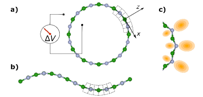
The underlying physical model is that of a nanotube of radius constructed by bending a flat layer, as illustrated in Fig.1(a); the voltage drop between the interior and the exterior is then given by Eq. (1). Another obvious example is that of a long-wavelength flexural phonon [see Fig. 1(b)]. Due to rotational invariance, the modulated strain field locally recovers the same pattern as in Fig.1(a). [See Ref. Stengel, 2013a and Sec. 2.8.2 of Ref. Stengel and Vanderbilt, 2016.] At the leading order in the wave vector, this results in a local jump in the electrostatic potential across the layer of
| (2) |
where the local inverse radius of curvature, , is given by the Laplacian of the vertical displacement field, . See Supplemental Material at http://link for more information about theoretical derivations, computational details and results, which includes Refs. [39-48]. As we shall see shortly, the effect originates from the distortion of both the electronic cloud and the crystal structure [Fig.1(c)].
To express the flexovoltage as a linear-response property, we start by associating the flexural deformation with a mapping between the Cartesian frame of the flat layer, and the curvilinear frame of the bent nanotube [dashed grid in Fig.1(a)]. In a neighborhood of the nanotube surface, such a mapping corresponds to a strain field with cylindrical symmetry, of the type , where is the normal to the layer surface, runs over the tangential direction, and is the symmetric strain tensor. This results in a macroscopic transverse strain gradient whose amplitude is the inverse radius of curvature, Stengel (2014); Stengel and Vanderbilt (2016) and will play the role of the perturbative parameter, , henceforth.
To discuss the electrostatic potential, which defines the open-circuit voltage , we shall frame our arguments on the Poisson equation in the curvilinear frame of the bent layer, following the guidelines of Refs. Stengel, 2013a, 2014; Stengel and Vanderbilt, 2016,
| (3) |
The main difference with respect to the Cartesian formulation is that the vacuum permittivity here becomes a tensor that depends on the metric of the deformation, . Within the linear regime, one can write , where is the unperturbed density and the first-order response in . (For the time being we shall assume that refers to the static response, inclusive of electronic and ionic relaxations.) We find that the open-circuit potential is given by
| (4) |
where
| (5) |
indicate the first (dipolar) and second (quadrupolar) moment of the function along the out-of-plane direction , and and are the in-plane averages of the respective microscopic response functions. corresponds to the -derivative of the “radial polarization” () as defined in Ref. Codony et al., 2021; the second term in Eq. (4) is a metric contribution that only depends on the unperturbed density , and originates from the linear variation of in Eq. (3). As we shall see shortly, the dipolar linear-response part is always large and negative, while the metric term is large and positive, typically leading to an almost complete mutual cancellation.
The challenging part of the problem consists in computing the dipolar linear-response contribution. To facilitate our progress towards a practical method, we shall use , where is the microscopic polarization response to the deformation. (The zero-th moment of along yields , after an integration by parts.) Then, by using the formulation of Ref. Stengel (2013a), we can write the radial component of as
| (6) |
The cell-periodic response functions and (in-plane averaging is assumed) have the physical interpretation of a local piezoelectric (U) and flexoelectric (G) coefficient. Stengel (2014) The rationale behind such a decomposition is rooted on the availability of efficient first-principles methods to calculate both terms in Eq. (6), as we shall illustrate in the following.
To perform the actual calculations, we shall accommodate the unperturbed (flat) monolayer in a standard supercell, where the out-of-plane dimension is treated as a convergence parameter. Regarding the gradient (G) contribution, we find
| (7) |
where is the out-of-plane component of the macroscopic dielectric tensor, and is the transverse component of the flexoelectric tensor of the supercell. Clearly, both and depend on (averaging over an arbitrary supercell volume is implied, and short-circuit electrical boundary conditions are usually imposed Royo and Stengel (2019) in the calculation of ). However, they do so in such a way that their ratio multiplied by does not (assuming that is large enough to consider the repeated layers as nonoverlapping). Regarding the contribution of the first term on the rhs of Eq. (6), we have
| (8) |
where is the first-order charge-density response to a uniform strain (). The total flexovoltage of the slab is then given by
| (9) |
where neither of , or depend on , and should therefore be regarded as well-defined physical properties of the isolated monolayer. One can verify that, by applying the present formulation to crystalline slabs of increasing thickness, we recover the results of Ref. Stengel, 2014 once is divided by the slab thickness, , and the thermodynamic limit performed. ( and tend to the bulk and surface contributions to the total flexoelectric effect, respectively.)
Eq. (9) is directly suitable for a numerical implementation, as it only requires response functions that are routinely calculated within density-functional perturbation theory (DFPT). The partition between “G” and “U” contributions, however, is hardly meaningful for an atomically thin 2D monolayer, where essentially everything is surface and there is no bulk underneath. Thus, we shall recast Eq. (9) in a more useful form hereafter, by seeking a separation between clamped-ion (CI) and lattice-mediated (LM) effects instead [Fig. 1(b)],
| (10) |
We find See Supplemental Material at http://link for more information about theoretical derivations, computational details and results, which includes Refs. [39-48]. that the CI contribution has the same functional form as the total response,
| (11) |
with the only difference that the flexoelectric (), dielectric () and uniform-strain charge response () functions have been replaced here with their clamped-ion counterparts, indicated by barred symbols. Regarding the LM part,
| (12) |
we have a more intuitive description in terms of the out-of-plane longitudinal charges , the pseudoinverse Hong and Vanderbilt (2013) of the zone-center dynamical matrix, , and the atomic force response See Supplemental Material at http://link for more information about theoretical derivations, computational details and results, which includes Refs. [39-48]. to a flexural deformation of the slab, . Note that the “mixed” contribution Stengel (2013b) to the bulk flexoelectric tensor exactly cancels See Supplemental Material at http://link for more information about theoretical derivations, computational details and results, which includes Refs. [39-48]. with an equal and opposite term in the lattice-mediated contribution to , hence its absence from Eq. (10).
| C | 0.1134 | 0.0000 | 0.1134 |
|---|---|---|---|
| Si | 0.0585 | 0.0000 | 0.0585 |
| P (zigzag) | 0.2320 | 0.0151 | 0.2170 |
| P (armchair) | 0.0130 | 0.0461 | 0.0591 |
| BN | 0.0381 | 0.1628 | 0.2009 |
| MoS2 | 0.2704 | 0.0565 | 0.3269 |
| WSe2 | 0.3158 | 0.0742 | 0.3899 |
| SnS2 | 0.1864 | 0.1728 | 0.3592 |
Our calculations are performed in the framework of density-functional perturbation theory Baroni et al. (2001); Gonze and Lee (1997) (DFPT) within the local-density approximation, as implemented in ABINIT Gonze et al. (2009); Romero et al. (2020). (Computational parameters and extensive tests, including calculations performed within the generalized-gradient approximation, are described in Ref. See Supplemental Material at http://link for more information about theoretical derivations, computational details and results, which includes Refs. [39-48]., ). In Table 1 we report the calculated bending flexovoltages for several monolayer crystals. Both the CI and LM contributions show a considerable variety in magnitude and sign: while the former dominates in the TMDs, the reverse is true for BN, and SnS2 seems to lie right in the middle. The case of phosphorene is interesting: its lower symmetry allows for a nonzero in spite of it being an elemental crystal like C and Si; it also allows for a substantial anisotropy of the response. If we assume a physical thickness corresponding to the bulk interlayer spacing, we obtain an estimate (see Table 6 of Ref. See Supplemental Material at http://link for more information about theoretical derivations, computational details and results, which includes Refs. [39-48]., ) for the volume-averaged flexoelectric coefficients, of pC/m. (, unlike , is inappropriate Codony et al. (2021) for 2D layers given the ill-defined nature of the parameter ; we use it here for comparison purposes only.) This value is in the same ballpark as earlier predictions, Shi et al. (2018); Zhuang et al. (2019); Pandey et al. (2021a, b) although there is a considerable scatter in the latter. For example, the value quoted by Ref. Zhuang et al. (2019) for graphene is very close to ours, but their results for other materials are either much larger (TMD’s, silicene) or much smaller (BN); other works tend to disagree both with our results and among themselves. These large discrepancies are likely due to the specific computational methods that were adopted in each case (often the total dipole moment of a bent nanoribbon including the boundaries was calculated, rather than the intrinsic response of the extended layer), or to the aforementioned difficulties Codony et al. (2021) with the definition of the dipole of a curved surface.
Very recently Ref. Codony et al. (2021) reported first-principles calculations of some of the materials presented here by using methods that bear some similarities to ours, which allows for a more meaningful comparison. By converting our results for Si and C to the units of Ref. Codony et al. (2021) via Eq. (1), we obtain and ; these, however, are almost two orders of magnitude smaller, and with inconsistent signs, with respect to the corresponding results of Ref. Codony et al. (2021). We ascribe the source of disagreement to the neglect in Ref. Codony et al. (2021) of the metric term in Eq. (11). Indeed, for the dipolar linear-response contribution [first two terms in Eq. (11)] we obtain and , now in excellent agreement (except for the sign) with the results of Codony et al.. This observation points to a nearly complete cancellation between the dipolar and metric contribution to , which is systematic across the whole materials set (see Table 3 of Ref. See Supplemental Material at http://link for more information about theoretical derivations, computational details and results, which includes Refs. [39-48]. ).
To clarify this point, we have performed additional calculations on toy model, consisting of a hexagonal layer of well-spaced rare gas atoms. See Supplemental Material at http://link for more information about theoretical derivations, computational details and results, which includes Refs. [39-48]. This is a system where no response should occur, as an arbitrary “mechanical deformation” consists in the trivial displacement of noninteracting (and spherically symmetric) neutral atoms. We find that and are, like in other cases, large and opposite in sign; this, however, is just a side-effect of the coordinate transformation (i.e., a mathematical artefact), and does not reflect a true physical response of the system to the perturbation. For a lattice parameter that is large enough, the cancellation becomes exact and our calculated value of vanishes as expected on physical grounds. This further corroborates the soundness of our definition of , which is based on the electrostatic potential. The latter, in addition to being an experimentally relevant parameter, behaves as a true scalar under a coordinate transformation; it is therefore unaffected, unlike the charge density, by the (arbitrary) choice of the reference frame. See Supplemental Material at http://link for more information about theoretical derivations, computational details and results, which includes Refs. [39-48].
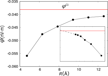
As a further consistency check, we have performed explicit calculations of BN nanotubes of increasing radius , and extracted the voltage drop between their interior and exterior, , at the clamped-ion level. In Figure 2 we plot the estimated flexovoltage, given by , as a function of . The asymptotic convergence to the linear-response value of is clear, consistent with Eq. (1). The convergence rate, however, appears rather slow: at the largest value of , corresponding to a nanotube primitive cell of 128 atoms, the deviation from is still of about 10%. This result highlights the difficulties at calculating flexovoltages in 2D systems by using the direct approach; conversely, our method provides an optimally converged solution within few minutes on a modern workstation, and is ideally suited, e.g. for high-throughput screening applications.
The implications of our findings for the interpretation of the experiments are best discussed in terms of the interaction between the flexural modes of a flat layer and an external, generally inhomogeneous, out-of-plane electric field, . In full generality, Eq. (2) leads to the following coupling (energy per unit area),
| (13) |
which reduces to for monochromatic fields of the type [. By deriving with respect to the displacement we obtain the converse flexoelectric effect, in the form of a vertical force per unit area, , in response to the field. Explicit first-principles calculations of a BN layer under an applied See Supplemental Material at http://link for more information about theoretical derivations, computational details and results, which includes Refs. [39-48]. nicely confirm this prediction: Eq. (13) is the main source of out-of-plane electromechanical response in this class of materials. Note that the longitudinal out-of-plane flexoelectric coefficient of a free-standing layer, which we extract as a by-product of our main calculations, always vanishes (see Ref. See Supplemental Material at http://link for more information about theoretical derivations, computational details and results, which includes Refs. [39-48]., ) due to translational invariance and thus cannot contribute to the coupling, contrary to the common belief. Brennan et al. (2017, 2020).
This allows us to generalize the existing models Amorim and Guinea (2013) of supported 2D layers by incorporating flexoelectricity, and thereby extract two important messages. See Supplemental Material at http://link for more information about theoretical derivations, computational details and results, which includes Refs. [39-48]. First, the amplitude of the response is highly sensitive to the substrate interaction strength, , consistent with the results of recent measurements performed on suspended layers. Wang et al. (2019b) Second, the response displays a strong dispersion in , indicating a marked sensitivity on the length scale of the inhomogeneities in the applied field. Both outcomes call for a reinterpretation of the existing PFM measurements of flexoelectricity: Brennan et al. (2017) information about and the tip geometry appears essential for a quantitative estimation of . We hope that our results will stimulate further experimental research along these lines, and more generally to facilitate the design of piezoelectric nanocomposites Chu et al. (2009) based on the flexoelectric effect.
Acknowledgements.
We acknowledge the support of Ministerio de Economia, Industria y Competitividad (MINECO-Spain) through Grants No. MAT2016-77100-C2-2-P and No. SEV-2015-0496, and of Generalitat de Catalunya (Grant No. 2017 SGR1506). This project has received funding from the European Research Council (ERC) under the European Union’s Horizon 2020 research and innovation program (Grant Agreement No. 724529). Part of the calculations were performed at the Supercomputing Center of Galicia (CESGA).References
- Wu et al. (2014) Wenzhuo Wu, Lei Wang, Yilei Li, Fan Zhang, Long Lin, Simiao Niu, Daniel Chenet, Xian Zhang, Yufeng Hao, Tony F. Heinz, James Hone, and Zhong Lin Wang, “Piezoelectricity of single-atomic-layer MoS2 for energy conversion and piezotronics,” Nature 514, 470–474 (2014).
- Ahmadpoor and Sharma (2015) Fatemeh Ahmadpoor and Pradeep Sharma, “Flexoelectricity in two-dimensional crystalline and biological membranes,” Nanoscale 7, 16555–16570 (2015).
- Kalinin and Meunier (2008) Sergei V. Kalinin and Vincent Meunier, “Electronic flexoelectricity in low-dimensional systems,” Phys. Rev. B 77, 033403 (2008).
- McGilly et al. (2020) Leo J. McGilly, Alexander Kerelsky, Nathan R. Finney, Konstantin Shapovalov, En-Min Shih, Augusto Ghiotto, Yihang Zeng, Samuel L. Moore, Wenjing Wu, Yusong Bai, Kenji Watanabe, Takashi Taniguchi, Massimiliano Stengel, Lin Zhou, James Hone, Xiaoyang Zhu, Dmitri N. Basov, Cory Dean, Cyrus E. Dreyer, and Abhay N. Pasupathy, “Visualization of Moiré superlattices,” Nature Nanotechnology 15, 580–584 (2020).
- Naumov et al. (2009) Ivan Naumov, Alexander M. Bratkovsky, and V. Ranjan, “Unusual flexoelectric effect in two-dimensional noncentrosymmetric -bonded crystals,” Phys. Rev. Lett. 102, 217601 (2009).
- Duerloo et al. (2012) Karel-Alexander N. Duerloo, Mitchell T. Ong, and Evan J. Reed, “Intrinsic piezoelectricity in two-dimensional materials,” The Journal of Physical Chemistry Letters 3, 2871–2876 (2012).
- Brennan et al. (2017) Christopher J. Brennan, Rudresh Ghosh, Kalhan Koul, Sanjay K. Banerjee, Nanshu Lu, and Edward T. Yu, “Out-of-plane electromechanical response of monolayer molybdenum disulfide measured by piezoresponse force microscopy,” Nano Letters 17, 5464–5471 (2017).
- Brennan et al. (2020) Christopher J. Brennan, Kalhan Koul, Nanshu Lu, and Edward T. Yu, “Out-of-plane electromechanical coupling in transition metal dichalcogenides,” Applied Physics Letters 116, 053101 (2020).
- Zubko et al. (2013) P. Zubko, G. Catalan, and A. K. Tagantsev, “Flexoelectric effect in solids,” Annu. Rev. Mater. Res. 43, 387–421 (2013).
- Wang et al. (2019a) Bo Wang, Yijia Gu, Shujun Zhang, and Long-Qing Chen, “Flexoelectricity in solids: Progress, challenges, and perspectives,” Progress in Materials Science 106, 100570 (2019a).
- Wang et al. (2019b) Xiang Wang, Anyang Cui, Fangfang Chen, Liping Xu, Zhigao Hu, Kai Jiang, Liyan Shang, and Junhao Chu, “Probing effective out-of-plane piezoelectricity in van der waals layered materials induced by flexoelectricity,” Small 15, 1903106 (2019b).
- Jungk et al. (2007) T. Jungk, Á. Hoffmann, and E. Soergel, “Influence of the inhomogeneous field at the tip on quantitative piezoresponse force microscopy,” Applied Physics A 86, 353–355 (2007).
- Shi et al. (2018) Wenhao Shi, Yufeng Guo, Zhuhua Zhang, and Wanlin Guo, “Flexoelectricity in monolayer transition metal dichalcogenides,” The Journal of Physical Chemistry Letters 9, 6841–6846 (2018).
- Shi et al. (2019) Wenhao Shi, Yufeng Guo, Zhuhua Zhang, and Wanlin Guo, “Strain gradient mediated magnetism and polarization in monolayer VSe2,” J. Phys. Chem. C 123, 24988–24993 (2019).
- Pandey et al. (2021a) T. Pandey, L. Covaci, and F.M. Peeters, “Tuning flexoelectricty and electronic properties of zig-zag graphene nanoribbons by functionalization,” Carbon 171, 551–559 (2021a).
- Pandey et al. (2021b) T. Pandey, L. Covaci, M. V. Milošević, and F. M. Peeters, “Flexoelectricity and transport properties of phosphorene nanoribbons under mechanical bending,” Phys. Rev. B 103, 235406 (2021b).
- Zhuang et al. (2019) Xiaoying Zhuang, Bo He, Brahmanandam Javvaji, and Harold S. Park, “Intrinsic bending flexoelectric constants in two-dimensional materials,” Phys. Rev. B 99, 054105 (2019).
- Javvaji et al. (2019) Brahmanandam Javvaji, Bo He, Xiaoying Zhuang, and Harold S. Park, “High flexoelectric constants in janus transition-metal dichalcogenides,” Phys. Rev. Materials 3, 125402 (2019).
- Codony et al. (2021) David Codony, Irene Arias, and Phanish Suryanarayana, “Transversal flexoelectric coefficient for nanostructures at finite deformations from first principles,” Phys. Rev. Materials 5 (2021), 10.1103/physrevmaterials.5.l030801.
- Stengel (2013a) M. Stengel, “Microscopic response to inhomogeneous deformations in curvilinear coordinates,” Nature Communications 4, 2693 (2013a).
- Cross (2006) L. Eric Cross, “Flexoelectric effects: Charge separation in insulating solids subjected to elastic strain gradients,” Journal of Materials Science 41, 53–63 (2006).
- Yudin and Tagantsev (2013) P. V. Yudin and A. K. Tagantsev, “Fundamentals of flexoelectricity in solids,” Nanotechnology 24, 432001 (2013).
- Resta (2010) Raffaele Resta, “Towards a bulk theory of flexoelectricity,” Phys. Rev. Lett. 105, 127601 (2010).
- Stengel (2013b) M. Stengel, “Flexoelectricity from density-functional perturbation theory,” Phys. Rev. B 88, 174106 (2013b).
- Stengel and Vanderbilt (2016) Massimiliano Stengel and David Vanderbilt, “First-principles theory of flexoelectricity,” in Flexoelectricity in Solids From Theory to Applications, edited by Alexander K. Tagantsev and Petr V. Yudin (World Scientific Publishing Co., Singapore, 2016) Chap. 2, pp. 31–110.
- Dreyer et al. (2018) Cyrus E. Dreyer, Massimiliano Stengel, and David Vanderbilt, “Current-density implementation for calculating flexoelectric coefficients,” Phys. Rev. B 98, 075153 (2018).
- Schiaffino et al. (2019) Andrea Schiaffino, Cyrus E. Dreyer, David Vanderbilt, and Massimiliano Stengel, “Metric wave approach to flexoelectricity within density functional perturbation theory,” Phys. Rev. B 99, 085107 (2019).
- Royo and Stengel (2019) Miquel Royo and Massimiliano Stengel, “First-principles theory of spatial dispersion: Dynamical quadrupoles and flexoelectricity,” Phys. Rev. X 9, 021050 (2019).
- Romero et al. (2020) Aldo H. Romero, Douglas C. Allan, Bernard Amadon, Gabriel Antonius, Thomas Applencourt, Lucas Baguet, Jordan Bieder, François Bottin, Johann Bouchet, Eric Bousquet, Fabien Bruneval, Guillaume Brunin, Damien Caliste, Michel Côté, Jules Denier, Cyrus Dreyer, Philippe Ghosez, Matteo Giantomassi, Yannick Gillet, Olivier Gingras, Donald R. Hamann, Geoffroy Hautier, François Jollet, Gérald Jomard, Alexandre Martin, Henrique P. C. Miranda, Francesco Naccarato, Guido Petretto, Nicholas A. Pike, Valentin Planes, Sergei Prokhorenko, Tonatiuh Rangel, Fabio Ricci, Gian-Marco Rignanese, Miquel Royo, Massimiliano Stengel, Marc Torrent, Michiel J. van Setten, Benoit Van Troeye, Matthieu J. Verstraete, Julia Wiktor, Josef W. Zwanziger, and Xavier Gonze, “Abinit: Overview and focus on selected capabilities,” The Journal of Chemical Physics 152, 124102 (2020).
- Martin (1972) Richard M. Martin, “Piezoelectricity,” Phys. Rev. B 5, 1607–1613 (1972).
- (31) See Supplemental Material at http://link for more information about theoretical derivations, computational details and results, which includes Refs. [39-48]., .
- Stengel (2014) Massimiliano Stengel, “Surface control of flexoelectricity,” Phys. Rev. B 90, 201112 (2014).
- Hong and Vanderbilt (2013) Jiawang Hong and David Vanderbilt, “First-principles theory and calculation of flexoelectricity,” Phys. Rev. B 88, 174107 (2013).
- Baroni et al. (2001) S. Baroni, S. de Gironcoli, and A. Dal Corso, “Phonons and related crystal properties from density-functional perturbation theory,” Rev. Mod. Phys. 73, 515 (2001).
- Gonze and Lee (1997) X. Gonze and C. Lee, “Dynamical matrices, Born effective charges, dielectric permittivity tensors, and interatomic force constants from density-functional perturbation theory,” Phys. Rev. B 55, 10355 (1997).
- Gonze et al. (2009) X. Gonze, B. Amadon, P.-M. Anglade, J.-M. Beuken, F. Bottin, P. Boulanger, F. Bruneval, D. Caliste, R. Caracas, M. Côté, T. Deutsch, L. Genovese, Ph. Ghosez, M. Giantomassi, S. Goedecker, D.R. Hamann, P. Hermet, F. Jollet, G. Jomard, S. Leroux, M. Mancini, S. Mazevet, M.J.T. Oliveira, G. Onida, Y. Pouillon, T. Rangel, G.-M. Rignanese, D. Sangalli, R. Shaltaf, M. Torrent, M.J. Verstraete, G. Zerah, and J.W. Zwanziger, “ABINIT: First-principles approach to material and nanosystem properties,” Computer Phys. Commun. 180, 2582–2615 (2009).
- Amorim and Guinea (2013) Bruno Amorim and Francisco Guinea, “Flexural mode of graphene on a substrate,” Phys. Rev. B 88, 115418 (2013).
- Chu et al. (2009) Baojin Chu, Wenyi Zhu, Nan Li, and L. Eric Cross, “Flexure mode flexoelectric piezoelectric composites,” Journal of Applied Physics 106, 104109 (2009).
- Royo et al. (2020) Miquel Royo, Konstanze R Hahn, and Massimiliano Stengel, “Using high multipolar orders to reconstruct the sound velocity in piezoelectrics from lattice dynamics,” Phys. Rev. Lett. 125, 217602 (2020).
- Hamann (2013) D. R. Hamann, “Optimized norm-conserving vanderbilt pseudopotentials,” Phys. Rev. B 88, 085117 (2013).
- van Setten et al. (2018) M.J. van Setten, M. Giantomassi, E. Bousquet, M.J. Verstraete, D.R. Hamann, X. Gonze, and G.-M. Rignanese, “The PseudoDojo: Training and grading a 85 element optimized norm-conserving pseudopotential table,” Comp. Phys. Comm. 226, 39–54 (2018).
- Novoselov et al. (2016) K.S. Novoselov, A. Mishchenko, A. Carvalho, and A.H. Castro Neto, “2d materials and van der waals heterostructures,” Science 353, aac9439 (2016).
- Pike et al. (2017) Nicholas A. Pike, Benoit Van Troeye, Antoine Dewandre, Guido Petretto, Xavier Gonze, Gian-Marco Rignanese, and Matthieu J. Verstraete, “Origin of the counterintuitive dynamic charge in the transition metal dichalcogenides,” Phys. Rev. B 95, 201106 (2017).
- Perdew et al. (1996) John P. Perdew, Kieron Burke, and Matthias Ernzerhof, “Generalized gradient approximation made simple,” Phys. Rev. Lett. 77, 3865–3868 (1996).
- Hamann et al. (2005) D.R. Hamann, Karin M. Rabe, and David Vanderbilt, “Generalized-gradient-functional treatment of strain in density-functional perturbation theory,” Phys. Rev. B 72 (2005), 10.1103/physrevb.72.033102.
- Jain et al. (2013) Anubhav Jain, Shyue Ping Ong, Geoffroy Hautier, Wei Chen, William Davidson Richards, Stephen Dacek, Shreyas Cholia, Dan Gunter, David Skinner, Gerbrand Ceder, and Kristin A. Persson, “The materials project: A materials genome approach to accelerating materials innovation,” APL Materials 1, 011002 (2013).
- Royo and Stengel (2020) Miquel Royo and Massimiliano Stengel, “Exact long-range dielectric screening and interatomic force constants in quasi-2d crystals,” Physical Review X (accepted), arXiv preprint arXiv:2012.07961 (2020).
- Kumar and Suryanarayana (2020) Shashikant Kumar and Phanish Suryanarayana, “Bending moduli for forty-four select atomic monolayers from first principles,” Nanotechnology 31, 43LT01 (2020).