Local and global properties of energy transfer in models of plasma turbulence

Abstract

The nature of the turbulent energy transfer rate is studied using direct numerical simulations of weakly collisional space plasmas. This is done comparing results obtained from hybrid Vlasov-Maxwell simulations of colissionless plasmas, Hall-magnetohydrodynamics, and Landau fluid models reproducing low-frequency kinetic effects, such as the Landau damping. In this partially developed turbulent scenario, estimates of the local and global scaling properties of different energy channels are obtained using a proxy of the local energy transfer (LET). This approach provides information on the structure of energy fluxes, under the assumption that the turbulent cascade transfers most of the energy that is then dissipated at small scales by various kinetic processes in this kind of plasmas.

1 Introduction

Space plasmas are a unique laboratory to study the transfer of energy in highly turbulent media (Bruno & Carbone, 2016). In particular, the Solar Wind near the Earth has been continuously probed by space missions (Tu & Marsch, 1995). The in situ measurements of this quasi-collisionless, highly variable, and structured plasma show a medium in a state of fully-developed turbulence. Under these conditions, turbulence is primarily originated at the Sun, and transported at high speed away from the source (Goldstein et al., 1996). This turbulence is then dissipated through magnetohydrodynamic (MHD)- to kinetic-scales, where processes as plasma waves excitation (e.g. (Pezzi et al., 2013)), temperature anisotropy (e.g., (Servidio et al., 2012; Perrone et al., 2014a)), plasma heating (e.g., (Smith et al., 2001; Perrone et al., 2014b; Vaivads et al., 2016)), particle energization (e.g., (Gibelli et al., 2010)), entropy cascade (e.g., (Cerri et al., 2018; Yang et al., 2017)), and enstrophy cascade (e.g., (Servidio et al., 2008)) are activated. Consequently, this energy cascade produces finer structures in the particles velocity distribution function (VDF) (Marsch et al., 2004; Valentini et al., 2008; Vásconez et al., 2014).

The MHD approximation describes space plasmas phenomenology at large enough scales (Servidio et al., 2008). In this approach, a Kolmogorov-like behaviour is highly supported by observations of velocity and magnetic fluctuations showing power-law spectra and intermittency (Carbone et al., 2004; Greco et al., 2009). At the MHD scales, the Solar Wind has shown scale-dependent non-Gaussian statistics (Sorriso-Valvo et al., 1999), with non-Gaussian fluctuations observed as well in the large scales (Marino et al., 2012) as it happens also in anisotropic fluids with waves (Feraco et al., 2018). Then, its turbulent energy is dissipated in an efficient way as a result of the inhomogeneous energy transfer, mostly occurring at small-scale vorticity filaments, rotational (or tangential) discontinuities, and current sheets, among other structures (Zimbardo et al., 2010). At scales close the proton inertial length and/or to the proton skin depth, pure MHD models are no longer valid (Matthaeus et al., 2008). Kinetic processes, led by field-particle interactions, have to be considered. Observations at $1$AU show non-Maxwelliam VDFs of ions and electrons in the zone where a low collisions rate is measured (Leamon et al., 1998). Complementary to the observations, Vlasov-Maxwell numerical simulations have confirmed that particles energization is taking place near the most intense small-scale structures (Servidio et al., 2015). The processes responsible for such energization are not yet understood. However, mechanisms as magnetic reconnection (e.g., (Servidio et al., 2009)), plasma instabilities (e.g., (Primavera et al., 2019; Settino et al., 2020)), wave-particle interactions (e.g. (Sorriso-Valvo et al., 2019; Chen et al., 2019) and increase of collisions (e.g., (Pezzi et al., 2016, 2017)) have been pointed out as good candidates. Then, direct numerical simulations have reveled to be quite useful to understanding the physics of the plasmas under conditions of the near-Earth Solar Wind.

In this work, we study the properties of the turbulent energy transfer in plasmas in the direct numerical simulations (DNS) framework previously investigated in Perrone et al. (2018). In their work, Hall-magnetohydrodynamic (HMHD), Landau Fluid (LF), and hybrid Vlasov-Maxwell (HVM) bidimensional simulations in turbulent regimes were ran under collisionless-plasma conditions, considering an out-of-plane ambient magnetic field. Magnetic diffusivity was carefully introduced in the fluid models. The fields obtained from these simulations allow us to explore different scales linked to their respective range of validity.

This paper is organized as follows. In Section 2, we briefly present the three numerical models, namely HMHD, LF and HVM, which describe –under the same 2D configuration– a collisionless plasma, in typical conditions of the Solar-Wind plasma, in a quasi-developed turbulent state. Our analysis of local and global energy transfer of this state is shown in Section 3 and Section 4, respectively. We summarize and conclude in Section 5.

2 Numerical models

The dynamical behavior of a plasma strongly depends on its frequencies. Here, we provide a very brief description of the three models used in the present work, which can properly focus on different ranges of frequency. At the lowest frequencies, where ions and electrons are locked together, and the plasma behaves like an electrically conducting fluid, a MHD model is good enough to describing the system. In this study, we use a HMHD simulation, which retains dispersive effects that become relevant at scales comparable to the proton skin depth. However, when collisions can be neglected, pressure anisotropy can develop in the plasma. In this case, and at somewhat higher frequency than the previous regime, a two-fluid description is needed, since electrons and ions can move relatively to each other. Therefore, we use a LF model which is able to take into account both pressure anisotropy and low-frequency kinetic effects, such as Landau damping. At higher frequencies, a kinetic model is required. We consider the HVM approach which describes the evolution of the proton distribution function, while electrons are treated as a fluid. All the three models include the electron inertial effects with a protons-to-electron mass ratio $m_{p}/m_{e}=100$.

The HMHD and LF codes use a 2D Fourier pseudo-spectral method to compute the spatial derivatives, while the time advance is performed with a third-order Runge-Kutta scheme. In these fluid codes, aliasing errors in the evaluation of nonlinear terms are treated by a $2/3$ truncation in the spectral space. In the HVM code, time advance is based on the time-splitting scheme (Cheng & Knorr, 1976), combined with the Current Advance Method –CAM (Matthews, 1994). In the Vlasov equation, advection in space and velocity are solved through an explicit upwind scheme (Van Leer, 1977). The HVM code uses FFT’s operations only when computing their fields, and truncation is not needed since possible dealiasing errors are damped by the intrinsic dissipation of the numerical scheme.

The vector fields will evolve in a double periodic domain $D=[L,L]$, in the $(x,y)$ plane. $L=2\pi\times 25d_{p}$ is the length of each direction $x$ and $y$. This domain is discretized with $N_{x}=N_{y}=1024$ grid points. Additionally, the HVM simulation is run in a 3D velocity domain $-5v_{th,p}\leq{\bf v}\leq 5v_{th,p}$, discretized with $51^{3}$ points, and where $v_{th,p}$ is the thermal velocity of the protons. At $t=0$, the equilibrium was set by a homogeneous plasma embedded in an uniform background magnetic field, ${\bf B}_{0}=(0,0,B_{0})$, oriented in the $z$-direction. The initial perturbation of this equilibrium is performed by velocity (and magnetic) field fluctuations with random phases in the interval $2\leq m\leq 6$, for the wavenumbers $k=2\pi m/L$. Although the amplitude of the magnetic perturbations are $b/B_{0}\approx 0.3$, no density fluctuations neither parallel variances are imposed. In fluid models, a magnetic diffusivity term with a coefficient $\eta=2\times 10^{-2}$ has been added.

2.1 Hall-magnetohydrodynamic

The HMHD model includes the electron inertia contribution. The adimensional set of equations is

$$\frac{\partial n}{\partial t}+\nabla\cdot(n{\bf u})=0;$$ (1)

$$\frac{\partial{\bf u}}{\partial t}+({\bf u}\cdot\nabla){\bf u}=-\frac{\beta}{2n}\nabla P+\frac{1}{n}\left[(\nabla\times{\bf B})\times{\bf B}\right];$$ (2)

$$\frac{\partial{\bf B}}{\partial t}=-\nabla\times{\bf E}+\eta\nabla^{2}{\bf B};$$ (3)

$$(1+\alpha\nabla^{2}){\bf E}+{\bf u}\times{\bf B}-\frac{1}{n}\left[(\nabla\times{\bf B})\times{\bf B}\right]=0;\\$$ (4)

$$P=n^{\gamma},$$ (5)

where $n$ is the plasma density, ${\bf u}$ is the hydrodynamic velocity, ${\bf E}$ and ${\bf B}$ are the electric and magnetic field, respectively. $P$ is the isotropic total pressure, $\eta=2\times 10^{-2}$ is the magnetic diffusivity, $\gamma=5/3$ is the adiabatic index, and $\alpha=1/100$ is an artificial electron to proton mass ratio. This adimensional set of equations are obtained normalizing $n$ to $n_{0}m_{p}$, ${\bf u}$ to the Alfvén speed $v_{A}$, $t$ to the inverse proton cyclotron frequency $\Omega_{cp}^{-1}$, and the length units to the proton skin depth $d_{p}=v_{A}/\Omega_{cp}$. For regularization purposes, and to reproduce the same-time behavior for the maximum value of the integrated parallel current density $\langle j_{z}^{2}\rangle$, bi-Laplacian hyperviscosity and hyperdiffusivity with coefficients equal to $5\times 10^{-4}$, have been added to the RHS of velocity and magnetic field equations.

2.2 Landau fluid

The LF system of dynamical equations is set for solving the evolution of the magnetic field, density, velocity, parallel and perpendicular pressures, and heat fluxes of the ions (Sulem & Passot, 2015). The electric field is computed using a generalized Ohm’s law, which includes the Hall term, together with electron inertia with the same simplified form and the same artificial mass ratio as in the HMHD case. The electron pressure gradient, which is formally present in the Ohm’s law, is here neglected to closely match the conditions of the Vlasov simulations, in which electrons are cold. The fluid hierarchy is closed by the gyrotropic fourth-rank moments in terms of the above quantities, in a way consistent with the low-frequency linear kinetic theory. In this study we are not considering the ion finite Larmor radius, and only ion linear Landau damping is retained, in the approximation discussed in (Passot et al., 2014). Together with the same hyperviscosity and hyperdiffusivity (as in HMHD equations), additional bi-Laplacian dissipative terms have been supplemented in the equations for the density and the pressures (with coefficient equal to $2.5\times 10^{-3}$), and in the equations for the ion heat flux (with coefficient $10^{-4}$) in order to deal with the high level of compressibility in the simulation (the Mach number reaching values up to $0.4$). In fact, we note that compressibility of these fluid models will be important when comparing our results.

2.3 Hybrid Vlasov-Maxwell

The hybrid Vlasov-Maxwell (HVM) code (Valentini et al., 2007) solves the Vlasov equation for the protons distribution function $f=f({\bf r},{\bf v},t)$, while the electrons response is taken into account through a generalized Ohm’s law for the electric field. The Vlasov equation, in normalized units,

$$\frac{\partial f}{\partial t}+{\bf v}\cdot\frac{\partial f}{\partial{\bf r}}+({\bf E}+{\bf u}_{p}\times{\bf B})\cdot\frac{\partial f}{\partial{\bf v}}=0,$$ (6)

is solved in a 2D-3V phase-space domain (two dimensions in physical space, and three dimensions in velocity space), coupling it with equations (3), and (4). Velocities ${\bf v}$ and ${\bf u}_{p}$ (protons bulk velocity) are scaled to $v_{A}$. Quasi-neutrality ($n=n_{e}=n_{p}$), and cold electrons, is considered. The time step is chosen in order to satisfy the Courant-Friedrichs-Lewy (CFL) condition for the numerical stability. Protons distribution function is initialized with a homogeneous-density Maxwellian function. In this procedure, displacement current is neglected in the Ampère law, making the assumption of low frequencies.

3 Local energy transfer analysis

The analysis developed in this work will be performed in a period of maximal turbulence activity. As described in Perrone et al. (2018), this state is reached at $t^{*}=60\Omega_{cp}^{-1}$, for the same set of simulations considered here. They established $t^{*}$ after following $\langle j_{z}^{2}\rangle$ in time, for HMHD, LF, and HVM descriptions, where the same $\beta$ was hold in order to ensure similar level of density fluctuations.

Figure 1 shows the spectra of ${\bf B}$ and ${\bf u}$, for the HMHD (left column), LF (middle column), and HVM (right column) simulations, respectively. Magnetic field spectra (bidimensional $|B(k_{x},k_{y})|^{2}$, and reduced integrated $|B_{ki}|^{2}$) are presented in the two-top rows, while the velocity field spectra (bidimensional $|u(k_{x},k_{y})|^{2}$, and reduced integrated $|u_{ki}|^{2}$) can be seen in the two-bottom rows. The integrated spectra are plotted respect to $k_{i}=k_{x}$ with a red-dashed line, and respect to $k_{i}=k_{y}$ with a black-solid line. Bidimensional spectra maps of HMHD, and LF simulations shows the $2/3$ truncation, which was not performed in the HVM simulation.

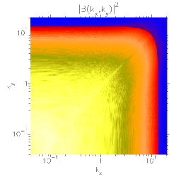
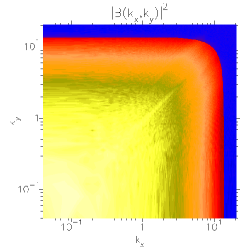
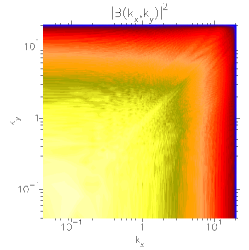
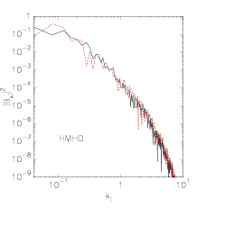
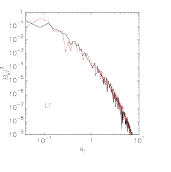
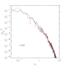
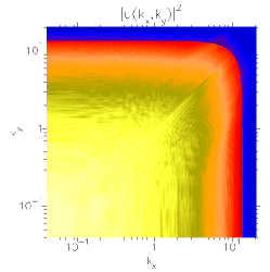
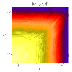
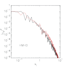
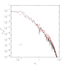
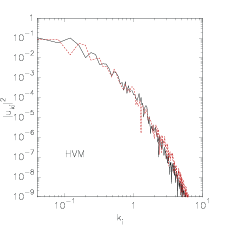
Figure 1: Magnetic field (two-top rows) and velocity field (two-bottom rows) spectra. The integrated spectra are presented respect to $k_{i}$, $i=x$ (red-dashed line), $y$ (black-solid line).

Considering that, in the small-scales limit, HMHD physics was observed to match hybrid-kinetic models results (e.g., (Vásconez et al., 2015; Pucci et al., 2016)), Hellinger et al. (2018) presented a generalization of the von Kármán-Howarth equation for incompressible hydrodynamic turbulence, in the framework of incompressible HMHD equations. This generalization was revisited by Ferrand et al. (2019), who also considered homogeneous turbulence, and worked with two-point correlation tensors depending only on the relative displacement ${\bf\ell}$, and not on the absolute positions, as $\delta{\bf f}={\bf f}({\bf r}+{\bf\ell})-{\bf f}({\bf r})$. In this context, the mean rate of total energy injection $\epsilon$ is expressed as the combination of the third-order structure functions corresponding to the MHD turbulent cascade flux (Carbone et al., 2009; Verdini et al., 2015), and to Hall corrections (e.g., (Galtier, 2008)).

$$-4\epsilon=\nabla\cdot\langle(\delta{\bf u}\cdot\delta{\bf u})\delta{\bf u}+(\delta{\bf B}\cdot\delta{\bf B})\delta{\bf u}-2(\delta{\bf u}\cdot\delta{\bf B})\delta{\bf B}-\frac{d_{p}}{2}(\delta{\bf B}\cdot\delta{\bf B})\delta{\bf j}+d_{p}(\delta{\bf B}\cdot\delta{\bf j})\delta{\bf B}\rangle.$$ (7)

In fact, we can identify the single contribution of each component that corresponds to the Yaglom-,

$${\bf Y}_{1}(x,y) = (\delta{\bf u}\cdot\delta{\bf u})\delta{\bf u};$$ (8)

$${\bf Y}_{2}(x,y) = (\delta{\bf B}\cdot\delta{\bf B})\delta{\bf u};$$ (9)

$${\bf Y}_{3}(x,y) = -2(\delta{\bf u}\cdot\delta{\bf B})\delta{\bf B},$$ (10)

and to the Hall-effect contributions,

$${\bf H}_{1}(x,y) = d_{p}(\delta{\bf B}\cdot\delta{\bf j})\delta{\bf B};$$ (11)

$${\bf H}_{2}(x,y) = -\frac{d_{p}}{2}(\delta{\bf B}\cdot\delta{\bf B})\delta{\bf j}.$$ (12)

In this way, equation 7 would be written as $-4\epsilon=\nabla\cdot\langle{\bf Y}_{1}+{\bf Y}_{2}+{\bf Y}_{3}+{\bf H}_{1}+{\bf H}_{2}\rangle$.

On the other hand, a heuristic proxy has been recently introduced. It focuses on the local turbulent energy transfer rate (LET) towards the smallest resolved scale. The proxy was constructed in order to extend the Yaglom law to MHD turbulence, and matches the latter law when small density fluctuations (at the scale $\ell$) can be neglected (Carbone et al., 2009). It is estimated, for 2D incompressible turbulence, through the combined third-order fluctuations of velocity, magnetic field, and current density (Sorriso-Valvo et al., 2018), and neglecting unity-order multiplicative factors, as

$$-2\ell\epsilon_{\ell}\equiv(\delta{\bf u}\cdot\delta{\bf u})\delta u_{\ell}+(\delta{\bf B}\cdot\delta{\bf B})\delta u_{\ell}-2(\delta{\bf u}\cdot\delta{\bf B})\delta B_{\ell}-\frac{d_{p}}{2}(\delta{\bf B}\cdot\delta{\bf B})\delta j_{\ell}+d_{p}(\delta{\bf B}\cdot\delta{\bf j})\delta B_{\ell}.$$ (13)

Consistently with our notation, the latter equation could be rewritten as

$$-2\ell\epsilon_{\ell}=\epsilon_{Y}+\epsilon_{H},$$ (14)

where $\epsilon_{Y}=\epsilon_{Y_{1}}+\epsilon_{Y_{2}}+\epsilon_{Y_{3}}$, and $\epsilon_{H}=\epsilon_{H_{1}}+\epsilon_{H_{2}}$. For this, $\epsilon_{Y_{1}}=(\delta{\bf u}\cdot\delta{\bf u})\delta u_{\ell}$ measures the kinetic energy available to be transported by the longitudinal component of $\delta{\bf u}$, $\epsilon_{Y_{2}}=(\delta{\bf B}\cdot\delta{\bf B})\delta u_{\ell}$ quantifies the magnetic energy that will be transported by $\delta u_{\ell}$, $\epsilon_{Y_{3}}=-2(\delta{\bf u}\cdot\delta{\bf B})\delta B_{\ell}$ is related to the velocity-magnetic field correlations coupled to the longitudinal magnetic field fluctuations, $\epsilon_{H_{1}}=-d_{p}(\delta{\bf B}\cdot\delta{\bf B})\delta j_{\ell}/2$ let us know the quantity of magnetic energy advected by longitudinal current-density field fluctuations, and $\epsilon_{H_{2}}=d_{p}(\delta{\bf B}\cdot\delta{\bf j})\delta B_{\ell}$ is related to the magnetic-current density field correlations coupled to the longitudinal magnetic field fluctuations. In equation 13, the two latter terms vanish when $d_{p}\to 0$, which recovers the classic Yaglom law.

Since we want to explore the energy flux distribution resulting from the turbulent nonlinear transfer, we first focus on the scale $\sim d_{p}$, i.e., at the bottom of the inertial range, where the intermittent structures carrying the most of the energy have been formed. As we noted in Section 2, $N_{x}=N_{y}=1024$, then $\Delta x=\Delta y\approx 0.15$, resulting in $\ell\approx 8$. At this scale, we will identify the Yaglom ${\bf Y}_{m}(x,y)=({\bf Y}_{mx}+{\bf Y}_{my})/2$, and Hall ${\bf H}_{n}(x,y)=({\bf H}_{nx}+{\bf H}_{ny})/2$ contributions, according to their spatial distribution, where $m=1,2,3$ and $n=1,2$. These bidimensional maps are presented in Figure 2 (HMHD), Figure 3 (LF), and Figure 4 (HVM). They clearly highlight the intermittent nature of the cross-scale energy transfer. This is evidenced by the presence of strong contributions to the scaling law in small-scale localized, sparse structures. Most of the energy transfer, and consequently of the energy dissipation, is taking place at those locations. It is interesting to note that different terms of the Hall-MHD law may present similar structures at the same locations. However, in several occasions the structures of different contributions are not co-located, suggesting that the nature of the fluctuations producing the energy transfer may be change with position, possibly enabling different dissipation mechanisms (Sorriso-Valvo et al., 2019). It is also apparent that most of the more intense structures are positive, suggesting that the energy is being transferred towards the small scales in a “direct” cascade. However, several negative structures are also present, where the contribution from the various terms is acting as to remove energy from the smaller scales. We do not imply here that the sign of the local contributions is related to the cascade direction, and the latest statements should be taken as a qualitative indication. Note that the overall energy flux will result from the average over the whole domain, and is mostly positive, as expected and as we shall discuss in the next Section. Comparing the different simulations reveals that the various terms have similar behaviour. In particular, the ${\bf Y}_{3}$ term seems to be dominating in the simulations. Interestingly, in the HMHD simulation the Hall terms appear weaker than in the two other simulations. This observation will be discussed later.

Finally, the maps of ${\bf Y}+{\bf H}$ are separated by components in Figure 5, for the HVM simulation (similar behavior was found in HMHD and LF simulations –not shown here). While the general behaviour is similar, some differences between the two components of the energy transfer exist, possibly an effect of the finite size of the ensemble.

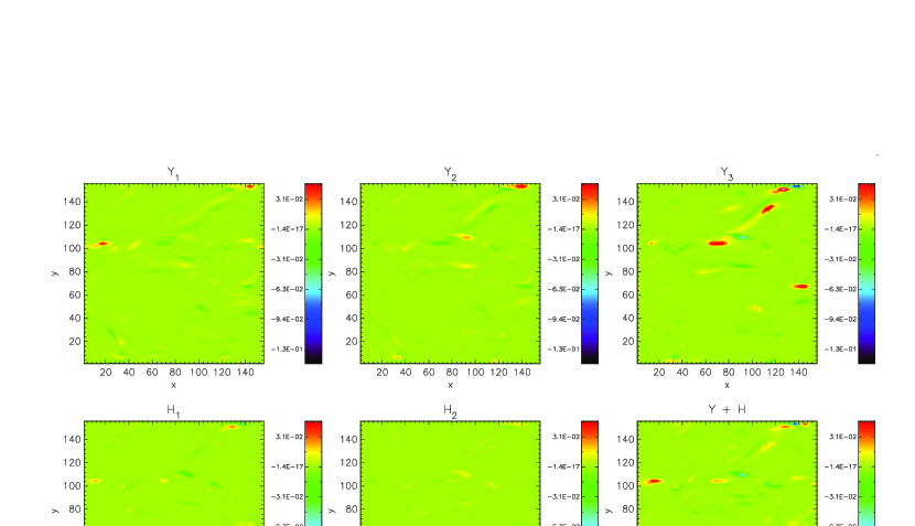
Figure 2: HMHD simulation. Bidimensional maps of Yaglom components: ${\bf Y}_{1}$ (Eq. 8), ${\bf Y}_{2}$ (Eq. 9), and ${\bf Y}_{3}$ (Eq. 10); and Hall components: ${\bf H}_{1}$ (Eq. 11), and ${\bf H}_{2}$ (Eq. 12), of the mean rate of total energy injection, estimated at the scale $\ell\simeq d_{p}$.

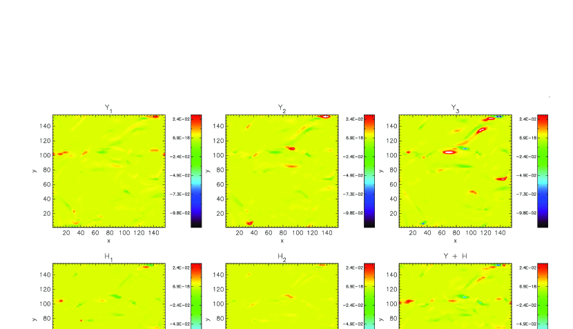
Figure 3: LF simulation. Bidimensional maps of Yaglom components: ${\bf Y}_{1}$ (Eq. 8), ${\bf Y}_{2}$ (Eq. 9), and ${\bf Y}_{3}$ (Eq. 10); and Hall components: ${\bf H}_{1}$ (Eq. 11), and ${\bf H}_{2}$ (Eq. 12), of the mean rate of total energy injection, estimated at the scale $\ell\simeq d_{p}$.

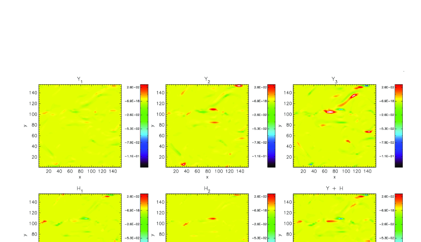
Figure 4: HVM simulation. Bidimensional maps of Yaglom components: ${\bf Y}_{1}$ (Eq. 8), ${\bf Y}_{2}$ (Eq. 9), and ${\bf Y}_{3}$ (Eq. 10); and Hall components: ${\bf H}_{1}$ (Eq. 11), and ${\bf H}_{2}$ (Eq. 12), of the mean rate of total energy injection, estimated at the scale $\ell\simeq d_{p}$.

Figure 5: $x$ (left panel) and $y$ (right panel) components of the term ${\bf Y}+{\bf H}$ (right panel), computed from the HVM simulation, estimated at the scale $\ell\simeq d_{p}$.

4 Global energy transfer analysis

We continue our analysis computing the local turbulent energy transfer rate $-2\epsilon_{\ell}$ across the scales $\ell$. The three panels of Figure 6 present the averaged equation (13) over the whole domain, corresponding to the HMHD (left panel), LF (middle panel), and HVM (right panel) simulations. We separate the Yaglom (black-solid line), and Hall (red-solid line) contributions in order to highlight their relative amplitude across the scales $\ell$. The sum of both contributions, giving the Hall-Yaglom law, is plotted with asterisks. As already observed in the previous Section, in the HMHD and LF simulations, the Hall contribution $\epsilon_{H(\ell)}$ is always lower than the Yaglom one. However, both contributions become closer for scales $\ell\lesssim d_{p}$. In the case of the HVM simulation, that occurs in the range $\ell\lesssim d_{p}$, $\epsilon_{H(\ell)}>\epsilon_{Y(\ell)}$. Then, at $\ell\approx d_{p}$, $\epsilon_{Y(\ell)}$ becomes more relevant and remains so for larger scales. This behavior is consistent with the settings of our simulations, where the mean field is out-of-plane, and there is strong whistler/magnetosonic activity. If we recall that the Hall term $\epsilon_{H}$ manifests itself through compressible activity, the cascade rates are expected to be affected in the fluid simulations; while in the HVM simulation, this compressible activity is suppressed through in-plane Landau damping and ion-cyclotron resonances, which re-inject in the system incompressible Alfvénic-like fluctuations. In this 2D setting, the LF model, in which Landau dissipation is introduced at a quasilinear level, partially quench compressible fluctuations but not as efficiently as the HVM one. In addition, we can confirm that in the interval $2d_{p}\lesssim\ell\lesssim 10d_{p}$ (roughly corresponding to the MHD-turbulence range), the scaling of $-2\epsilon_{\ell}$ is compatible with a linear scaling law (black-dashed line) for our three cases of study, as previously reported by Sorriso-Valvo et al. (2018).

Figure 6: Cascade rate $-2\epsilon_{\ell}$ law as a function of the scale $\ell$, conducted in the HMHD (left panel), LF (middle panel), and HVM (right panel) simulations. The contributing terms: $\epsilon_{Y}$ (black-solid line), and $\epsilon_{H}$ (red-solid line) are presented together to their direct sum (asterisks). The dashed line represents the linear scaling.

Moreover, in Figure 7 we can see how Yaglom $-\epsilon_{Y_{m}}$ and Hall $-\epsilon_{H_{n}}$ terms, respectively, are supporting the latter global behavior. We use black-empty diamonds to picture the positive terms, while negative quantities are plotted with red-filled diamonds. The left column shows HMHD-simulation results, middle column corresponds to the LF simulation, while the results from the HVM simulation are presented in the right column. If we focus on the amplitude and sign of these quantities, we cannot note substantial differences between the individual Hall-contributions among the simulations. However, the sign of $-\epsilon_{Y_{2}}$ (associated to the magnetic energy transported by the velocity field) is passing from negative to positive at $\sim 2d_{p}$ in the HVM simulation. This is not seen in their HMHD and LF counterparts.

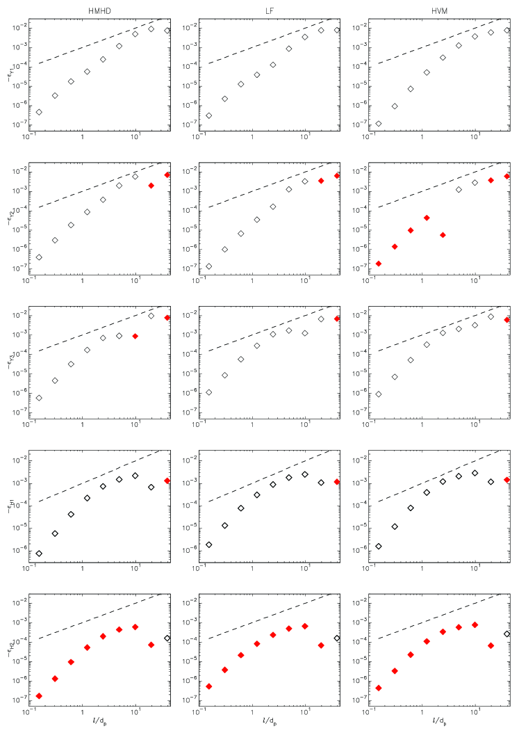
Figure 7: From top to bottom row: $-\epsilon_{Y_{1}}$, $-\epsilon_{Y_{2}}$, $-\epsilon_{Y_{3}}$, $-\epsilon_{H_{1}}$, and $-\epsilon_{H_{2}}$. The components are computed from the HMHD (left column), LF (middle column), and HVM (right column) simulations. Black-empty diamonds correspond to the positive sign, while red-filled diamonds show negative values. Linear scaling is plotted with a black-dashed line.

Finally, we use our results to compare the amplitude of each of Yaglom and Hall terms across the scales. In Figure 8, we present these comparisons for the Yaglom terms: $\epsilon_{Y_{1}}/\epsilon_{Y_{3}}$ (top-left panel), and $\epsilon_{Y_{2}}/\epsilon_{Y_{3}}$ (top-right panel). Hall terms comparison $\epsilon_{H_{1}}/\epsilon_{H_{2}}$ can be seen in the bottom-left panel. The bottom-right panel shows $\epsilon_{Y}/\epsilon_{H}$. Black-solid line is for HMHD simulation, blue-dash-dotted line represents the LF results, and the red-dashed line is for the HVM simulation. From a global point of view, we note that the comparisons computed from the LF and HVM simulations are quite similar, specially for scales $\ell\lesssim 10d_{p}$. After this range, the sign of $\epsilon_{Y_{3}}$ fluctuates with respect to that of $\epsilon_{Y_{1}}$ and $\epsilon_{Y_{2}}$. On the other hand, the sign of $\epsilon_{H_{1}}$, as compared with $\epsilon_{H_{2}}$, remains negative for all of the scales. Once again, LF and HVM simulations seem quite similar when comparing the Hall terms. The comparison $\epsilon_{Y}/\epsilon_{H}$ shows that the HVM simulation is useful to study the transition from fluid to kinetic scales ($\sim d_{p}$) as we can see when comparing this ratio.

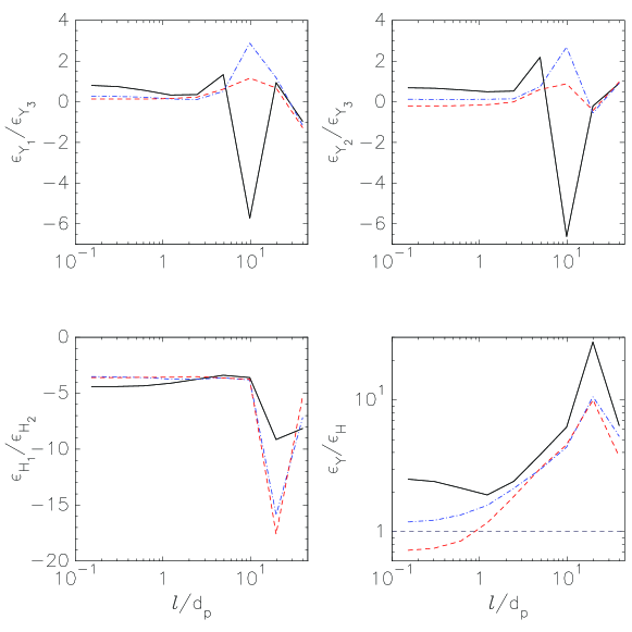
Figure 8: Comparison of the Yaglom terms $\epsilon_{Y_{1}}$ and $\epsilon_{Y_{2}}$, respect to $\epsilon_{Y_{3}}$ (top row). The comparison between the Hall terms ($\epsilon_{H_{1}}$ and $\epsilon_{H_{2}}$) is plotted in the bottom-left panel. The bottom-right panel shows the comparison between $\epsilon_{Y}$ and $\epsilon_{H}$. In the latter panel, the horizontal grey-dashed line marks the barrier of $\epsilon_{Y}/\epsilon_{H}=1$. Black-solid line corresponds to the HMHD simulation, blue-dash-dotted line shows the LF simulation, and HVM simulation is represented by the red-dashed line.

5 Discussion and Conclusions

In this paper we studied the properties of energy transfer contributions in collisionless turbulent plasmas. For this scope, the heuristic proxy LET was computed on three numerical simulations (Hall-MHD, Landau Fluid, and hybrid kinetic Vlasov-Maxwell) of a quasi-steady state of turbulence. Moreover, this study would also be aligned to the “Turbulent dissipation challenge” (Parashar et al., 2015), as we test the LET proxy on three different numerical models (which use different numerical schemes) under the same initial conditions, with similar physical and numerical parameters. We have in mind that each of these models have their own characteristic scale. In the HVM model, this scale corresponds to the proton skin depth. In the fluid models this scale corresponds to the dissipative scale, where the energy is dissipated by viscous and resistive effects.
From Figure 2 to Figure 4, we presented bi-dimensional maps for each of the simulations, and for the scale $\ell=8$ ($\sim d_{p}$). In particular, in Figure 5 we can show the location and intensity of the structures where most of the energy is contributing to the cross-scale transfer.
Then, Figure 6 tests the $-2\epsilon_{\ell}$ cascade-rate definition (equation (13)). Here, when only the global contribution of $\epsilon_{Y}+\epsilon_{H}$ is plotted (asterisks), no strong differences are seen between our set of simulations. However, when $\epsilon_{Y}$ (black-solid line) and $\epsilon_{H}$ (red-solid line) are separated, we note that compressible activity, suppressed (through in-plane Landau damping and ion-cyclotron resonances) in the HVM simulation (right panel), let that $\epsilon_{H}>\epsilon_{Y}$ for scales $\ell\lesssim d_{p}$. This is not reported in fluid-like simulations because $\epsilon_{H}$ is manifested mainly by the compressible activity. We further point out that a net contribution in the energy budget might be due to the pressure anisotropy, which is not taken into account in the fluid-Yaglom theory.
We observe that $\epsilon_{Y_{2}}\sim(\delta{\bf B}\cdot\delta{\bf u})\delta u_{\ell}$ have opposite sign –for the majority of the scales– in the HVM simulation, with respect to the fluid simulations (Figure 5). Also for this parameter, a change of monotony may be noticed in the interval $2d_{p}\lesssim\ell\lesssim 10d_{p}$ (roughly corresponding to the MHD-turbulence range), only in the HVM simulation. The reason for this behavior is not fully understood.
Finally, the comparisons made in Figure 8 show similitude between our set of simulations for scales $\ell\lesssim 2d_{p}$. After this range, the contribution of $\epsilon_{Y_{3}}$ decreases with respect to $\epsilon_{Y_{1}}$ (left-top panel) and $\epsilon_{Y_{2}}$ (right-top panel). A similar behavior, related to the direction of the energy cascade, is seen when comparing the Hall terms (left-bottom panel), where the amplitude of $\epsilon_{H_{2}}$ decreases more about one decade respect to $\epsilon_{H_{1}}$ when $\ell\gtrsim 10d_{p}$.
Our overall conclusion is that the three simulations are similar, but not exactly identical, with respect to the local and global turbulent energy transfer. This implies that a cross-scale interconnection exists between fluid and kinetic dynamics, so that not only the turbulent cascade drives the small-scale kinetic processes, but the latter also control the cascade, acting as a form of dynamical dissipation. Further studies are needed to describe in more details such interconnection. Work in progress includes the extension of energy-transfer analysis in 3D simulations, and a multifractal study of the turbulence (Primavera & Florio, 2019).

CLV was partially supported by EPN projects: PIM-19-01, PII-DFIS-2019-01 and PII-DFIS-2019-04.

References

- Bruno & Carbone (2016) Bruno, Roberto & Carbone, Vincenzo 2016 Turbulence in the solar wind .
- Carbone et al. (2004) Carbone, Vincenzo, Bruno, Roberto, Sorriso-Valvo, Luca & Lepreti, Fabio 2004 Intermittency of magnetic turbulence in slow solar wind. Planetary and Space Science 52 (10), 953–956.
- Carbone et al. (2009) Carbone, V, Marino, R, Sorriso-Valvo, L, Noullez, A & Bruno, R 2009 Scaling laws of turbulence and heating of fast solar wind: the role of density fluctuations. Physical review letters 103 (6), 061102.
- Carbone et al. (2009) Carbone, V., Sorriso-Valvo, L. & Marino, R. 2009 On the turbulent energy cascade in anisotropic magnetohydrodynamic turbulence. EPL (Europhysics Letters) 88 (2), 25001.
- Cerri et al. (2018) Cerri, SS, Kunz, Matthew Walter & Califano, F 2018 Dual phase-space cascades in 3d hybrid-vlasov–maxwell turbulence. The Astrophysical Journal Letters 856 (1), L13.
- Chen et al. (2019) Chen, CHK, Klein, KG & Howes, Gregory G 2019 Evidence for electron landau damping in space plasma turbulence. Nature communications 10 (1), 1–8.
- Cheng & Knorr (1976) Cheng, Chio-Zong & Knorr, Georg 1976 The integration of the vlasov equation in configuration space. Journal of Computational Physics 22 (3), 330–351.
- Feraco et al. (2018) Feraco, F, Marino, R, Pumir, A, Primavera, L, Mininni, PD, Pouquet, A & Rosenberg, D. 2018 Vertical drafts and mixing in stratified turbulence: sharp transition with froude number. Europhysics Letters 123, 4402.
- Ferrand et al. (2019) Ferrand, R., Galtier, S., Sahraoui, F., Meyrand, R., Andrés, N. & Banerjee, S. 2019 On exact laws in incompressible hall magnetohydrodynamic turbulence. The Astrophysical Journal 881 (1), 50.
- Galtier (2008) Galtier, Sébastien 2008 von kármán-howarth equations for hall magnetohydrodynamic flows. Physical Review E 77 (1), 015302, arXiv: 0712.1525.
- Gibelli et al. (2010) Gibelli, Livio, Shizgal, Bernie D & Yau, AW 2010 Ion energization by wave–particle interactions: Comparison of spectral and particle simulation solutions of the vlasov equation. Computers & Mathematics with Applications 59 (8), 2566–2581.
- Goldstein et al. (1996) Goldstein, BE, Neugebauer, M, Phillips, JL, Bame, S, Gosling, JT, McComas, D, Wang, YM, Sheeley, NR & Seuss, ST 1996 Ulysses plasma parameters: Latitudinal, radial, and temporal variations .
- Greco et al. (2009) Greco, A, Matthaeus, WH, Servidio, S, Chuychai, P & Dmitruk, P 2009 Statistical analysis of discontinuities in solar wind ace data and comparison with intermittent mhd turbulence. The Astrophysical Journal Letters 691 (2), L111.
- Hellinger et al. (2018) Hellinger, Petr, Verdini, Andrea, Landi, Simone, Franci, Luca & Matteini, Lorenzo 2018 von kármán–howarth equation for hall magnetohydrodynamics: Hybrid simulations. The Astrophysical Journal 857 (2), L19.
- Leamon et al. (1998) Leamon, Robert J, Smith, Charles W, Ness, Norman F, Matthaeus, William H & Wong, Hung K 1998 Observational constraints on the dynamics of the interplanetary magnetic field dissipation range. Journal of Geophysical Research: Space Physics 103 (A3), 4775–4787.
- Marino et al. (2012) Marino, R, Sorriso-Valvo, L, D’Amicis, R, Carbone, V, Bruno, R & Veltri, P 2012 On the occurrence of the third-order scaling in high latitude solar wind. The Astrophysical Journal 750, 41.
- Marsch et al. (2004) Marsch, E, Ao, X-Z & Tu, C-Y 2004 On the temperature anisotropy of the core part of the proton velocity distribution function in the solar wind. Journal of Geophysical Research: Space Physics 109 (A4).
- Matthaeus et al. (2008) Matthaeus, WH, Servidio, S & Dmitruk, P 2008 Comment on “kinetic simulations of magnetized turbulence in astrophysical plasmas”. Physical review letters 101 (14), 149501.
- Matthews (1994) Matthews, Alan P 1994 Current advance method and cyclic leapfrog for 2d multispecies hybrid plasma simulations. Journal of Computational Physics 112 (1), 102–116.
- Parashar et al. (2015) Parashar, Tulasi N, Salem, Chadi, Wicks, Robert T, Karimabadi, H, Gary, S Peter & Matthaeus, William H 2015 Turbulent dissipation challenge: a community-driven effort. Journal of Plasma Physics 81 (5).
- Passot et al. (2014) Passot, T, Henri, P, Laveder, D & Sulem, PL 2014 Fluid simulations of ion scale plasmas with weakly distorted magnetic fields. European Physical Journal D 68, 207.
- Perrone et al. (2014a) Perrone, D, Bourouaine, S, Valentini, F, Marsch, E & Veltri, P 2014a Generation of temperature anisotropy for alpha particle velocity distributions in solar wind at 0.3 au: Vlasov simulations and helios observations. Journal of Geophysical Research: Space Physics 119 (4), 2400–2410.
- Perrone et al. (2018) Perrone, D, Passot, T, Laveder, D, Valentini, F, Sulem, PL, Zouganelis, I, Veltri, P & Servidio, S 2018 Fluid simulations of plasma turbulence at ion scales: Comparison with vlasov-maxwell simulations. Physics of Plasmas 25 (5), 052302.
- Perrone et al. (2014b) Perrone, Denise, Valentini, Francesco, Servidio, Sergio, Dalena, Serena & Veltri, Pierluigi 2014b Analysis of intermittent heating in a multi-component turbulent plasma. The European Physical Journal D 68 (7), 209.
- Pezzi et al. (2017) Pezzi, O, Malara, F, Servidio, S, Valentini, F, Parashar, TN, Matthaeus, WH & Veltri, P 2017 Turbulence generation during the head-on collision of alfvénic wave packets. Physical Review E 96 (2), 023201.
- Pezzi et al. (2016) Pezzi, Oreste, Parashar, Tulasi N, Servidio, Sergio, Valentini, Francesco, Malara, Francesco, Matthaeus, William H & Veltri, Pierluigi 2016 Alfvénic wave packets collision in a kinetic plasma. EGUGA pp. EPSC2016–5663.
- Pezzi et al. (2013) Pezzi, Oreste, Valentini, Francesco, Perrone, Denise & Veltri, Pierluigi 2013 Eulerian simulations of collisional effects on electrostatic plasma waves. Physics of Plasmas 20 (9), 092111.
- Primavera & Florio (2019) Primavera, Leonardo & Florio, Emilia 2019 Parallel algorithms for multifractal analysis of river networks. In International Conference on Numerical Computations: Theory and Algorithms, pp. 307–317. Springer.
- Primavera et al. (2019) Primavera, Leonardo, Malara, Francesco, Servidio, Sergio, Nigro, Giuseppina & Veltri, Pierluigi 2019 Parametric instability in two-dimensional alfvénic turbulence. The Astrophysical Journal 880 (2), 156.
- Pucci et al. (2016) Pucci, F., Vásconez, C. L., Pezzi, O., Servidio, S., Valentini, F., Matthaeus, W. H. & Malara, F. 2016 From alfvén waves to kinetic alfvén waves in an inhomogeneous equilibrium structure. Journal of Geophysical Research: Space Physics 121 (2), 1024–1045, arXiv: https://agupubs.onlinelibrary.wiley.com/doi/pdf/10.1002/2015JA022216.
- Servidio et al. (2008) Servidio, S, Matthaeus, WH & Dmitruk, P 2008 Depression of nonlinearity in decaying isotropic mhd turbulence. Physical review letters 100 (9), 095005.
- Servidio et al. (2009) Servidio, S, Matthaeus, WH, Shay, MA, Cassak, PA & Dmitruk, P 2009 Magnetic reconnection in two-dimensional magnetohydrodynamic turbulence. Physical review letters 102 (11), 115003.
- Servidio et al. (2012) Servidio, S, Valentini, F, Califano, Francesco & Veltri, P 2012 Local kinetic effects in two-dimensional plasma turbulence. Physical review letters 108 (4), 045001.
- Servidio et al. (2015) Servidio, S, Valentini, F, Perrone, D, Greco, A, Califano, Francesco, Matthaeus, WH & Veltri, P 2015 A kinetic model of plasma turbulence. Journal of Plasma Physics 81 (1).
- Settino et al. (2020) Settino, A, Malara, F, Pezzi, O, Onofri, M, Perrone, D & Valentini, F 2020 Proton kinetics in kelvin-helmholtz instability. arXiv preprint arXiv:2005.09308 .
- Smith et al. (2001) Smith, Charles W, Matthaeus, William H, Zank, Gary P, Ness, Norman F, Oughton, Sean & Richardson, John D 2001 Heating of the low-latitude solar wind by dissipation of turbulent magnetic fluctuations. Journal of Geophysical Research: Space Physics 106 (A5), 8253–8272.
- Sorriso-Valvo et al. (1999) Sorriso-Valvo, Luca, Carbone, Vincenzo, Veltri, Pierluigi, Consolini, Giuseppe & Bruno, Roberto 1999 Intermittency in the solar wind turbulence through probability distribution functions of fluctuations. Geophysical Research Letters 26 (13), 1801–1804.
- Sorriso-Valvo et al. (2019) Sorriso-Valvo, Luca, Catapano, Filomena, Retinò, Alessandro, Le Contel, Olivier, Perrone, Denise, Roberts, Owen W, Coburn, Jesse T, Panebianco, Vincenzo, Valentini, Francesco, Perri, Silvia & others 2019 Turbulence-driven ion beams in the magnetospheric kelvin-helmholtz instability. Physical review letters 122 (3), 035102.
- Sorriso-Valvo et al. (2018) Sorriso-Valvo, Luca, Perrone, Denise, Pezzi, Oreste, Valentini, Francesco, Servidio, Sergio, Zouganelis, Ioannis & Veltri, Pierluigi 2018 Local energy transfer rate and kinetic processes: the fate of turbulent energy in two-dimensional hybrid vlasov–maxwell numerical simulations. Journal of Plasma Physics 84 (2).
- Sulem & Passot (2015) Sulem, P. L. & Passot, T. 2015 Landau fluid closures with nonlinear large-scale finite larmor radius corrections for collisionless plasmas. Journal of Plasma Physics 81 (1), 325810103.
- Tu & Marsch (1995) Tu, C-Y & Marsch, Eckart 1995 Mhd structures, waves and turbulence in the solar wind: Observations and theories. Space Science Reviews 73 (1-2), 1–210.
- Vaivads et al. (2016) Vaivads, Andris, Retinò, Alessandro, Soucek, J, Khotyaintsev, Yu V, Valentini, F, Escoubet, C Philippe, Alexandrova, Olga, André, Mats, Bale, SD, Balikhin, M & others 2016 Turbulence heating observer–satellite mission proposal. Journal of Plasma Physics 82 (5).
- Valentini et al. (2007) Valentini, F, Trávníček, P, Califano, Francesco, Hellinger, Petr & Mangeney, André 2007 A hybrid-vlasov model based on the current advance method for the simulation of collisionless magnetized plasma. Journal of Computational Physics 225 (1), 753–770.
- Valentini et al. (2008) Valentini, F, Veltri, P, Califano, Francesco & Mangeney, A 2008 Cross-scale effects in solar-wind turbulence. Physical review letters 101 (2), 025006.
- Van Leer (1977) Van Leer, Bram 1977 Towards the ultimate conservative difference scheme iii. upstream-centered finite-difference schemes for ideal compressible flow. Journal of Computational Physics 23 (3), 263–275.
- Vásconez et al. (2015) Vásconez, C. L., Pucci, F, Valentini, F, Servidio, S, Matthaeus, WH & Malara, F 2015 Kinetic alfvén wave generation by large-scale phase mixing. The Astrophysical Journal 815 (1), 7.
- Vásconez et al. (2014) Vásconez, C. L., Valentini, F, Camporeale, E & Veltri, P 2014 Vlasov simulations of kinetic alfvén waves at proton kinetic scales. Physics of Plasmas 21 (11), 112107.
- Verdini et al. (2015) Verdini, Andrea, Grappin, Roland, Hellinger, Petr, Landi, Simone & Müller, Wolf Christian 2015 Anisotropy of the third-order structure functions in mhd turbulence. The Astrophysical Journal 804 (2), 119.
- Yang et al. (2017) Yang, Yan, Matthaeus, WH, Parashar, TN, Wu, P, Wan, M, Shi, Y, Chen, S, Roytershteyn, V & Daughton, W 2017 Energy transfer channels and turbulence cascade in vlasov-maxwell turbulence. Physical Review E 95 (6), 061201.
- Zimbardo et al. (2010) Zimbardo, G, Greco, A, Sorriso-Valvo, L, Perri, S, Vörös, Z, Aburjania, G, Chargazia, K & Alexandrova, O 2010 Magnetic turbulence in the geospace environment. Space science reviews 156 (1-4), 89–134.