Binary Choice with Asymmetric Loss in a Data-Rich Environment: Theory and an Application to Racial Justice

Abstract

We study the binary choice problem in a data-rich environment with asymmetric loss functions. The econometrics literature covers nonparametric binary choice problems but does not offer computationally attractive solutions in data-rich environments. The machine learning literature has many algorithms but is focused mostly on loss functions that are independent of covariates. We show that theoretically valid decisions on binary outcomes with general loss functions can be achieved via a very simple loss-based reweighting of the logistic regression or state-of-the-art machine learning techniques. We apply our analysis to racial justice in pretrial detention.

Keywords: binary outcomes, asymmetric losses, machine learning, cost-sensitive classification, pretrial detention.

1 Introduction

The downside risk and upside gains of many economic decisions are not symmetric. The importance of asymmetries in prediction problems arising in economics has been recognized for a long time; see Granger (1969), Manski and Thompson (1989), Granger and Pesaran (2000), Elliot and Timmermann (2016), and references therein. In this paper, we focus on binary choice problems in a data-rich environment with general loss functions. Hence, our analysis covers many life-changing decisions such as college admission, job hiring, pretrial release from jail, medical testing and treatment, which have become increasingly driven by automated algorithmic processes based on vast data inputs. It also covers many routine tasks such as fraud detection, spam filters, credit risk, etc. The topic has gained interest from a diverse set of fields, ranging from economics, computer science, to machine learning, among others, and depending on the discipline is also known as classification or screening problems.

The combination of high-dimensional data and general loss functions in binary decision problems is challenging and not well understood. Econometricians have studied nonparametric binary choice problems for a long time, but the literature does not offer computationally attractive solutions for high-dimensional datasets. The existing attempts to relax the strong parametric distributional assumptions result in non-smooth combinatorial optimization problems, also known as NP-hard problems. Indeed, the maximum score method of Manski (1975), or the extension to the asymmetric loss functions proposed by Elliot and Lieli (2013), leads to such NP-hard optimization problems which makes them computationally challenging in data-rich environments.

The machine learning (ML) literature has many computationally attractive algorithms that form the basis for much of the automated procedures that are implemented in practice, but it is mostly focused on symmetric loss functions that are independent of economic factors. In particular, the ML literature emphasizes the importance of smooth optimization and made significant advances in proposing smooth convex and computationally attractive relaxations for the binary classification problem. There are a number of contributions in the ML literature on the asymmetric losses and cost-sensitive classification, see Scott (2011, 2012) and references therein. However, this literature does not cover losses/utility functions of interest to economists, nor does it establish the statistical properties for specific ML methods. Many applications of interest to economists would involve the asymmetric covariate-driven losses for mistakes and pay-offs for correct decisions. Indeed, the economic costs/benefits of bail, lending, and other decisions naturally lead to covariate-driven asymmetries. Therefore, the available ML methods are of limited interest to economists.

The optimal decisions with general asymmetric covariate-driven loss functions typically yield covariate-driven threshold rules. This is the case for the general social planner setting studied by Rambachan, Kleinberg, Ludwig, and Mullainathan (2020) as well as the special cases studied by Corbett-Davies, Pierson, Feller, Goel, and Huq (2017) and Kleinberg, Ludwig, Mullainathan, and Rambachan (2018), among others. To the best of our knowledge, there is no theory that supports the empirical implementation involving either logistic regression, deep learning, boosting, support vector machines, or LASSO. We provide such a theory for all these types of estimators. In particular, one of the main contributions of our paper is to show that binary decisions with arbitrary loss functions can be achieved via a very simple reweighting of the logistic regression, or other state-of-the-art machine learning techniques, such as boosting or (deep) neural networks. We establish the theoretical guarantees for all these methods in the case of generic asymmetric loss functions.

The novel contribution of our paper is to propose a framework for machine learning binary choice with general asymmetries of interest to economists, described by a generic loss function $\ell(f(x),y,x)$ and a decision function $f(x)$, both driven by realized covariates/features $x$, where $y$ are realized binary outcomes. We show how the loss function should be mapped to weights and establish the supporting theoretical results for the cost-sensitive empirical risk minimization. To that end, we generalize the extensive literature on the symmetric binary classification, see Zhang (2004), Bartlett, Jordan and Mcauliffe (2006), Boucheron, Bousquet, and Lugosi (2005), Koltchinskii (2011), and references therein. The key difficulty is to introduce a theoretical setting that is compatible with the logistic, exponential, and hinge convexifying functions for generic covariate-driven losses. We do so via the formulation of Assumption 3.2 (iii), which nests the symmetric binary classification and the asymmetric false positive/negative mistakes considered in the previous literature as a special case.

The practical implementation of our procedure is remarkably simple, which we why it can be discussed here. The first ingredient comes from a policy/decision-maker who has to provide a quartet of loss functions pertaining to (a) true positives (denoted by $\ell_{1,1}(x)$), (b) true negatives ($\ell_{-1,-1}(x)$), (c) false positives ($\ell_{-1,1}(x)$) and last but not least (d) false negatives ($\ell_{1,-1}(x)$). Note that this not only implies the selection of functional forms, but also the selection of inputs $x,$ i.e., individual covariates. It is important to emphasize that the functions $\ell_{j,k}(x),j,k\in\{-1,1\}$ are typically not estimated. They are determined by either a utility/cost function of the social planner (policy/decision-maker), or are obtained through some type of cost-benefit analysis. Given these economic inputs, the task of econometrician is to compute weights from $\ell_{j,k}(x),j,k\in\{-1,1\}$ that will be applied to the classification procedures. Our theoretical analysis is agnostic about which method to use and we cover a typical collection of classification tools. Our theory shows that this very simple loss-based reweighting leads to valid binary decisions without strong distributional assumptions. In some cases, e.g., for deep learning, these decisions are optimal from the minimax point of view.

Regarding deep learning, our paper is also related to the recent work of Farrell, Liang and Misra (2021) who show that under weak assumptions the deep learning estimators of the regression function can achieve sufficiently fast convergence rates for the semiparametric inference. In contrast, our paper fills a different gap in the econometrics literature related to asymmetric binary decisions, or put it differently NP-hard utility maximization problems, for which we offer the first practical and scalable solution in data-rich environments.

The contributions of our paper must also be cast in the context of the ongoing debate about so-called algorithmic biases. As more and more decisions affecting our daily lives have become digitized and automated by data-driven algorithms, concerns have been raised regarding such biases. Gender and race are two leading examples. Cowgill and Tucker (2019) discuss the case of computer scientists at Amazon who developed powerful new technology to screen resumes and discovered the algorithm placed a negative coefficient on terms associated with women and as a result appeared to be amplifying and entrenching male dominance in the technology industry. Another example of gender discrimination is discussed by Datta, Tschantz, and Datta (2007) who study AdFisher, an automated tool that explores how user behaviors, Google’s ads, and Ad Settings interact. They found that setting the gender to female resulted in getting fewer instances of an ad related to high-paying jobs than setting it to male. The empirical application in our paper relates to racial biases in pretrial detention. Journalists at the news website ProPublica reported on a commercial software used by judges in Broward County, Florida, that helps to decide whether a person charged with a crime should be released from jail before their trial. They found that the software tool called COMPAS resulted in a disproportionate number of false positives for black defendants who were classified as high risk but subsequently not charged with another crime. We apply our covariate-driven classification methods to pretrial decisions with an emphasis on racial justice.

The paper is organized as follows. Section 2 introduces notation, describes the binary decision problem in terms of risk/payoff, and illustrates a convenient for us characterization of the optimal binary decision. Examples of several asymmetric binary decision problems are also provided. Section 3 covers the main convexification theorem and provides examples of convexifying functions. In Section 4, we provide the excess risk bounds for the binary decision rules constructed from the data and discuss several cases, including logistic regression, LASSO, and deep learning. Finally, we provide an empirical application pertaining to pretrial detention in Section 5 followed by conclusions. An Online Appendix provides supplementary theoretical results and discusses boosting, while the Supplementary Material presents Monte Carlo simulation results and some details regarding the empirical application; see https://arxiv.org/abs/2010.08463.

2 Binary decisions

Let $Y\in\{-1,1\}$ be the target variable and let $X\in\mathcal{X}\subset\mathbf{R}^{d}$ be covariates. A measurable function $f:\mathcal{X}\to\{-1,1\}$ is called the binary decision/choice/prediction. The decision-making process amounts to minimizing a risk function that describes its consequences in different states of the world

$$\mathcal{R}(f)=\mathbb{E}_{Y,X}[\ell(f(X),Y,X)],$$

where $\ell:\{-1,1\}^{2}\times\mathcal{X}\to\mathbf{R}$ is a loss function specified by the decision-maker. Note that the decision $f$ can be random and the expectation is taken with respect to the distribution of $(Y,X)$ only. The loss function can be asymmetric and may also depend on the covariates $X$, which is economically a more realistic scenario faced by the decision-maker than the one provided by the standard classification setting.

2.1 Some examples

In the Introduction, we alluded to many examples in economic decision making. To motivate the first example, we can think of a credit risk application, where with the false negative mistakes ($f(X)=-1$ and $Y=1$) the bank suffers a loss from the borrower’s default, while with the false positive mistakes ($f(X)=1$ and $Y=-1$), the bank simply foregoes its potential earnings. Moreover, the size of the loan and other economic factors may determine the loss:

Example 2.1 (Lending decisions).

Let $y\in\{-1,1\}$ be the default status ($=1$ if defaulted) and $f\in\{-1,1\}$ be the lending decision ($=-1$ if approved). Let $L(s,z)$ and $\Pi(s,z)$ be the loss and the profit functions, where $s\geq 0$ is the size of the loan, $z\in\mathbf{R}^{d-1}$ some other economic factors. The lender’s loss function could be $\ell(f,y,s,z)=L(s,z)\mathbbm{1}_{f=-1,y=1}-\Pi(s,z)\mathbbm{1}_{f=-1,y=-1}$.

As noted in the Introduction, an important policy debate pertains to the fairness and the discrimination bias of machine learning algorithms towards, e.g., low income groups, gender, or race. The following example suggests that the unfair treatment of individuals can be eliminated if the social planner assigns different weights to the social welfare or loss function, see also Rambachan, Kleinberg, Ludwig, and Mullainathan (2020):

Example 2.2 (Social planner with a disadvantaged group).

Let $x=(g,z)\in\mathbf{R}^{d}$ be a vector of covariates, where $g\in\{0,1\}$ is a binary indicator of a disadvantaged group and $z\in\mathbf{R}^{d-1}$ are some other covariates. The social planner’s loss function is $\ell(f(x),y,x)=\psi_{g}\ell(f(x),y,x)$, where $\psi_{g}>0$ are the social welfare weights placed upon individuals in group $g\in\{0,1\},$ and $\psi_{1}>\psi_{0}$ implies that outcomes associated with the disadvantaged group are valued more than outcomes associated with the rest of the population.

Related to Example 2.2, we could also consider the loss function $\ell(f(x),y,x)=\psi_{g}\mathbbm{1}_{f(x)=-1,y=1}+\varphi_{g}\mathbbm{1}_{f(x)=1,y=-1}$ with group-specific weights $\psi_{g},\varphi_{g}>0$ on false negative/positive mistakes. Computer scientists have focused on defining fairness-aware algorithms by imposing restrictions on $f.$ Often a formal criterion of fairness is defined, and a decision rule is developed to satisfy the criterion, e.g., the statistical parity across groups. We follow the economist’s arguments that fairness is naturally defined through welfare/losses.

In the remainder of the paper, we will continue to work with settings involving a generic vector of covariates $X\in\mathbf{R}^{d}$ which may contain the binary group membership variable $G\in\{0,1\}$ and some other covariates $Z\in\mathbf{R}^{d-1}$. The point worth keeping in mind, however, is that our framework covers much discussed preference-based notions of fairness characterized by general covariate-driven loss functions.

2.2 Optimal binary decision

Following the decision-theoretic perspective, we define the optimal binary decision as the one achieving the smallest risk

$$\mathcal{R}^{*}=\inf_{f:\mathcal{X}\to\{-1,1\}}\mathbb{E}[\ell(f(X),Y,X)],$$

where the minimization is done over all measurable functions $f:\mathcal{X}\to\{-1,1\}$. Note that this framework also covers the utility/welfare maximization problems, in which case, we can define $\ell(f(X),Y,X)=-U(f(X),Y,X)$, where $U(f(x),y,x)$ is a utility/welfare function of a binary decision $f(x)$ when the outcome is $Y=y$ and covariates are $X=x$.

The following proposition provides an alternative convenient for us characterization of the optimal binary decision; see Online Appendix Section B.1 for a proof.

Proposition 2.1.

The optimal binary decision $f^{*}$ solves

$$\inf_{f:\mathcal{X}\to\{-1,1\}}\mathbb{E}\left[\omega(Y,X)\mathbbm{1}_{-Yf(X)\geq 0}\right]$$

with $\omega(Y,X)\triangleq Ya(X)+b(X)$, $a(x)=\ell_{-1,1}(x)-\ell_{1,1}(x)+\ell_{-1,-1}(x)-\ell_{1,-1}(x)$, $b(x)=\ell_{-1,1}(x)-\ell_{1,1}(x)+\ell_{1,-1}(x)-\ell_{-1,-1}(x)$, and $\ell_{f,y}(x)\triangleq\ell(f,y,x)$.

Note that $a$ can be interpreted as a difference of net losses $\ell_{-1,1}-\ell_{1,1}$ and $\ell_{1,-1}-\ell_{-1,-1}$ from wrong decisions when $Y=1$ and $Y=-1$ respectively. Similarly, $b$ can be interpreted as a sum of two net losses. Proposition 2.1 shows that the optimal binary decision minimizes the objective function involving the indicator function $z\mapsto\mathbbm{1}_{z\geq 0}$, which is discontinuous and not convex. This leads to a difficult NP-hard empirical risk minimization problem

$$\inf_{f:\mathcal{X}\to\{-1,1\}}\frac{1}{n}\sum_{i=1}^{n}\omega(Y_{i},X_{i})\mathbbm{1}_{-Y_{i}f(X_{i})\geq 0}.$$

3 Convexification

3.1 Convexified excess risk

The purpose of this section is to convexify the binary decision problem with a generic loss function making it amenable to modern machine learning algorithms. It is easy to see that the risk function of a binary decision rule $f:\mathcal{X}\to\{-1,1\}$ can be written as

$$\mathcal{R}(f)=0.5\mathbb{E}\left[\omega(Y,X)\mathbbm{1}_{-Yf(X)\geq 0}\right]+\mathbb{E}[d(Y,X)]$$

with $d(y,x)=0.25(\ell_{1,1}(x)+\ell_{-1,1}(x))(1+y)+0.25(\ell_{1,-1}(x)+\ell_{-1,-1}(x))(1-y)-0.25\omega(y,x)$; see the proof of Proposition 2.1 in Online Appendix Section B.1. Replacing the indicator function with a convex function $\phi:\mathbf{R}\to\mathbf{R}$, we obtain the convexified risk

$$\mathcal{R}_{\phi}(f) =0.5\mathbb{E}[\omega(Y,X)\phi(-Yf(X))]+\mathbb{E}[d(Y,X)].$$

Therefore, minimizing the convexified risk amounts to solving

$$\inf_{f:\mathcal{X}\to\mathbf{R}}\mathbb{E}[\omega(Y,X)\phi(-Yf(X))].$$

Let $f^{*}_{\phi}$ be a solution to the convexified problem and let $\mathcal{R}^{*}_{\phi}=\inf_{f:\mathcal{X}\to\mathbf{R}}\mathcal{R}_{\phi}(f)$ be the optimal convexified risk. Next, we can define the excess convexified risk of a decision $f:\mathcal{X}\to\{-1,1\}$ as

$$\mathcal{R}_{\phi}(f)-\mathcal{R}_{\phi}^{*}=0.5\mathbb{E}\left[\omega(Y,X)\left(\phi(-Yf(X))-\phi(-Yf^{*}_{\phi}(X))\right)\right].$$ (1)

The excess convexified risk measures the deviation of the convexified risk of a given decision rule $f:\mathcal{X}\to\{-1,1\}$ from the optimal convexified risk and can be controlled. Unfortunately, the convexified excess risk tells us little about the performance of the binary decision in terms of the actual excess risk that the decision-maker cares about, namely:

$$\mathcal{R}(f)-\mathcal{R}^{*}=0.5\mathbb{E}\left[\omega(Y,X)\left(\mathbbm{1}_{-Yf(X)\geq 0}-\mathbbm{1}_{-Yf^{*}(X)\geq 0}\right)\right].$$

In the following subsection, we show that the excess risk is bounded from above by the convexified excess risk, a result that we refer to as the main convexification theorem.

3.2 Assumptions and main convexification theorem

Let $\eta(x)=\Pr(Y=1|X=x)$ be the conditional choice probability. We impose the following assumption on the conditional probability $\eta$ and the loss function:

Assumption 3.1.

(i) $\ell_{-1,1}(x)-\ell_{1,1}(x)\geq c_{b}$ and $\ell_{1,-1}(x)-\ell_{-1,-1}(x)\geq c_{b}$ a.s. over $x\in\mathcal{X}$ for some $c_{b}>0$; (ii) there exist $\epsilon>0$ such that $\epsilon\leq\eta(x)\leq 1-\epsilon$ a.s. over $x\in\mathcal{X}$; (iii) there exists $M<\infty$ such that $|\ell_{f,y}(x)|\leq M$ a.s. over $x\in\mathcal{X}$ for all $f,y\in\{-1,1\}$, where $\ell_{f,y}=\ell(f,y,x)$.

Assumption 3.1 (i) requires that the losses from wrong decisions exceed those of correct decisions. It ensures that weights are $\omega(Y,X)\geq 0$ a.s., so that the convexification is possible (ii) requires that $\eta(x)$ is non-degenerate for almost all states of the world $x\in\mathcal{X}$ and is often imposed in econometrics literature. (iii) requires that the loss function is bounded and is satisfied in our empirical application.

Next, we restrict the class of convexifying function $\phi$.

Assumption 3.2.

(i) $\phi:\mathbf{R}\to[0,\infty)$ is a convex and non-decreasing function with $\phi(0)=1$; (ii) there exists some $L<\infty$ such that $|\phi(z)-\phi(z^{\prime})|\leq L|z-z^{\prime}|$ for all $z,z^{\prime}$; (iii) there exist $C>0$ and $\gamma\in(0,1]$ such that for all $x,c\in(0,1)$, $\left|x-c\right|\leq C\left(x+c-2xc-\inf_{y\in\mathbf{R}}Q_{c}(x,y)\right)^{\gamma}$, where $Q_{c}(x,y)=x(1-c)\phi(-y)+(1-x)c\phi(y),x,y\in\mathbf{R}$.

Note that Assumption 3.2 is formulated in a way that it can be verified for the logistic, exponential, and hinge convexifications; see also Lemmas B.3, B.4, and B.5 in the Online Appendix. We focus on these three convexifications since they cover the majority of ML algorithms used in practice, including the (penalized) logistic regression, boosting, deep learning, and support vector machines. Note also that Assumption 3.2 does not impose any restrictions on the loss function $\ell$.

We will also use the following covariate-driven threshold rule defined by the asymmetry of the loss function $\ell:$

$$c(x)=\frac{\ell_{1,-1}(x)-\ell_{-1,-1}(x)}{\ell_{-1,1}(x)-\ell_{1,1}(x)+\ell_{1,-1}(x)-\ell_{-1,-1}(x)},$$

where $\ell_{f,y}(x)=\ell(f,y,x)$.

For $z\in\mathbf{R}$, put $\mathrm{sign}(z)=\mathbbm{1}_{z\geq 0}-\mathbbm{1}_{z<0}$. Our first result establishes the link between the optimal decision $f^{*}$ and the solution to the convexified risk minimization problem $f^{*}_{\phi}.$

Proposition 3.1.

Suppose that Assumption 3.1 (i) is satisfied. Then the optimal decision is $f^{*}(x)=\mathrm{sign}(\eta(x)-c(x))$. Moreover, under Assumptions 3.1 (ii) and 3.2 (i) if $\phi$ is differentiable, then $\mathrm{sign}(f^{*}_{\phi}(x))=f^{*}(x)$.

The optimal decision rule $f^{*}(x)=\mathrm{sign}(\eta(x)-c(x))$ is well-known, see Elliot and Lieli (2013) and references therein. More importantly, Proposition 3.1 shows that the optimal decision rule for the convexified problem that can be easily solved in practice coincides with $f^{*}$. The threshold $c(x)$ corresponds to the fraction of net losses from false positives in the total net losses, hence, the decision $f(x)=1$ is made whenever the choice probability $\Pr(Y=1|X=x)$ exceeds the fraction of false positive losses. Note that in the symmetric binary classification case $\ell_{1,-1}(x)=\ell_{-1,1}(x)=1$ and $\ell_{1,1}(x)=\ell_{-1,-1}(x)=0$, so that $c(x)=1/2$ and the optimal decision is $f^{*}(x)=1$ if $\Pr(Y=1|X=x)$ exceeds $\Pr(Y=0|X=x)$ and $f^{*}(x)=-1$ otherwise.

It is worth mentioning that our starting point is a fixed decision problem described by the loss function $\ell$, which in conjunction with $\eta$ determines the boundary separating the two decisions $\{x\in\mathcal{X}:\;\eta(x)-c(x)=0\}$. The following condition generalizes the so-called Tsybakov’s noise or margin condition, see Boucheron, Bousquet, and Lugosi (2005), and quantifies the complexity of the decision problem.

Assumption 3.3.

Suppose that there exist $\alpha\geq 0$ and $C_{m}>0$ such that

$$P_{X}\left(\{x:\;|\eta(x)-c(x)|\leq u\}\right)\leq C_{m}u^{\alpha},\qquad\forall u>0.$$

If $\alpha=0$, then Assumption 3.3 does not impose any restrictions as we can always take $C_{m}=1$, while larger values of $\alpha$ are more advantageous for classification. In the special case of the symmetric binary classification, $c(x)=1/2$, and the extreme case of $\alpha=\infty$ corresponds $\eta(x)=\Pr(Y=1|X=x)$ being bounded away from $1/2$. We refer to Boucheron, Bousquet, and Lugosi (2005), Section 5.2, for additional discussions of the margin condition as well as for equivalent formulations in the special case of the symmetric binary classification.

Our next result relates the convexified excess risk bound to the excess risk bound of the binary decision problem a generic loss function under the margin condition.

Theorem 3.1.

Suppose that Assumptions 3.1, 3.2, and 3.3 are satisfied. Then there exists $C_{\phi}<\infty$ such that for every measurable function $f:\mathcal{X}\to\mathbf{R}$

$$\mathcal{R}(\mathrm{sign}(f))-\mathcal{R}^{*}\leq C_{\phi}\left[\mathcal{R}_{\phi}(f)-\mathcal{R}_{\phi}^{*}\right]^{\frac{\gamma(\alpha+1)}{\gamma\alpha+1}}.$$

The formal proof of this result with the explicit expression for the constant $C_{\phi}$ appears in the Appendix. It is worth noting that our result nests the symmetric binary classification as a special case, see e.g. Zhang (2004), Theorem 2.1. Theorem 3.1 relates the excess risk of the sign of $f$ to the convexified risk of $f$ (note that the convexified risk is well-defined for arbitrary $f:\mathcal{X}\to\mathbf{R}$). Therefore, instead of solving the NP-hard empirical risk minimization problem, in practice, we can solve the following weighted classification problem

$$\inf_{f\in\mathscr{F}}\frac{1}{n}\sum_{i=1}^{n}\omega(Y_{i},X_{i})\phi(-Y_{i}f(X_{i})),$$

where $\mathscr{F}$ is a class of measurable functions $f:\mathcal{X}\to[-1,1]$, called soft decision. Note that we restrict the range of soft decision to $[-1,1]$ since the risk is determined by the sign of $f$ only.

3.3 Examples

We consider three examples of convexifying functions widely used in empirical applications. They are the logistic, exponential and hinge functions used respectively in the logistic regression, adaptive boosting, and the support vector machines; see Figure 1. Applying Theorem 3.1 allows us to implement suitably reweighted versions.

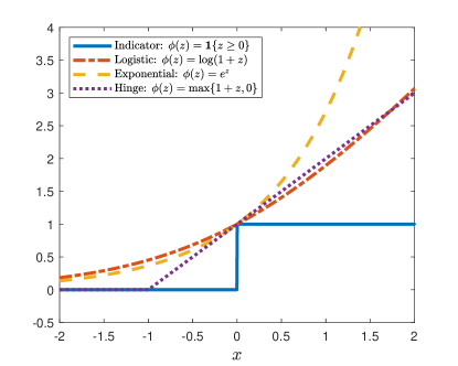
Figure 1: Convexifications corresponding to Logit, Boosting, and SVM.

Example 3.1 (Logistic convexification).

Lemma B.3 in the Online Appendix shows that the function $\phi(z)$ = $\log_{2}(1+e^{z})$ satisfies Assumption 3.2 with $\gamma=1/2$ and $C=\sqrt{2\log 2}$. The objective is to minimize $f\mapsto\frac{1}{n}\sum_{i=1}^{n}\omega(Y_{i},X_{i})\log_{2}\left(1+e^{-Y_{i}f(X_{i})}\right)$, which reduces to the logistic regression in the symmetric case.

The logistic convexifying function is also a default choice in several implementations of the gradient boosting, including the very popular state-of-the-art extreme gradient boosting (XGBoost) algorithm of Chen and Guestrin (2016) as well as the deep learning. This example, therefore, indicates that a suitably reweighted for the asymmetries of the loss function logistic regression, XGBoost, or deep learning can be used for economic decisions.

Example 3.2 (Exponential convexification).

Lemma B.5 in the Online Appendix shows that $\phi(z)$ = $\exp(z),$ the exponential convexifying function, satisfies Assumption 3.2 with $\gamma=1/2$ and $C={2}$. The objective is to minimize $f\mapsto\frac{1}{n}\sum_{i=1}^{n}\omega(Y_{i},X_{i})e^{-Y_{i}f(X_{i})}$, which reduces to the adaptive boosting (AdaBoost) in the symmetric case; see Friedman, Hastie, and Tibshirani (2001), Ch. 10.

This example, therefore, indicates that a loss-based reweighted adaptive boosting can be used for economic decisions.

Example 3.3 (Hinge convexification).

Lemma B.4 in the Online Appendix shows that $\phi(z)$ = $(1+z)_{+}$, the hinge convexifying function, satisfies Assumption 3.2 with $\gamma=1$ and $C=1$. The objective is to minimize $f\mapsto\frac{1}{n}\sum_{i=1}^{n}\omega(Y_{i},X_{i})(1-Y_{i}f(X_{i}))_{+}$, which reduces to the support vector machines in the symmetric case; see Friedman, Hastie, and Tibshirani (2001), Ch. 12.

This example, therefore, indicates that a loss-based reweighted support vector machines can be used for economic decisions.

4 Excess risk bounds

The convexified empirical risk minimization problem consists of minimizing the empirical risk

$$\widehat{\mathcal{R}}_{\phi}(f)=\frac{1}{n}\sum_{i=1}^{n}\omega(Y_{i},X_{i})\phi(-Y_{i}f(X_{i}))$$

over some class of functions $f:\mathcal{X}\to[-1,1]$, denoted $\mathscr{F}_{n}$. Let $\hat{f}_{n}$ be a solution to $\inf_{f\in\mathscr{F}_{n}}\widehat{\mathcal{R}}_{\phi}(f)$, and let $f_{n}^{*}$ be a solution to $\inf_{f\in\mathscr{F}_{n}}{\mathcal{R}}_{\phi}(f)$. Put also $\|f\|_{q}=(\mathbb{E}|f(X)|^{q})^{1/q}$ with $q\geq 1$ and $\|.\|_{2}=\|.\|$. The following assumption requires that the risk function is sufficiently curved around the minimizer.

Assumption 4.1.

There exist some $c_{\phi}>0$ and $\kappa\geq 1$ such that for every $f\in\mathscr{F}_{n}$

$$\mathcal{R}_{\phi}(f)-\mathcal{R}_{\phi}^{*}\geq c_{\phi}\|f-f^{*}_{\phi}\|^{2\kappa}.$$

It is worth mentioning that in light of Assumption 3.1 imposed on the loss function $\ell$, Assumption 4.1 is mainly about the curvature of the convexifying function $\phi$. In particular, it is typically satisfied with $\kappa=1$ when $\phi^{\prime\prime}$ is strictly positive, which is the case for the logistic and exponential convexifications; see Lemma B.7 in the Online Appendix. On the other hand, it holds with $\kappa=1+1/\alpha$ in the hinge case, where $\alpha$ is the margin parameter from the Assumption 3.3; see Lemma B.9. It is worth mentioning that the curvature condition in Assumption 4.1 is typically used to establish bounds on $\|f-f_{\phi}^{*}\|$ and may not be needed to establish the slow convergence rates of the excess risk. However, this condition is typically used to obtain the fast convergence rates for the excess risk in the symmetric classification and regression cases; see Koltchinskii (2011).

We first state the oracle inequality for the excess risk in terms of a fixed point of the local Rademacher complexity of the class $\mathscr{F}_{n}$ defined as

$$\psi_{n}(\delta;\mathscr{F}_{n})\triangleq\mathbb{E}\left[\sup_{f\in\mathscr{F}_{n}:\|f-f^{*}_{n}\|^{2}\leq\delta}|R_{n}(f-f^{*}_{n})|\right],$$

where $R_{n}(f-f_{n}^{*})=\frac{1}{n}\sum_{i=1}^{n}\varepsilon_{i}(f(X_{i})-f_{n}^{*}(X_{i}))$ is a Rademacher process, i.e., $(\varepsilon_{i})_{i=1}^{n}$ are i.i.d. in $\{-1,1\}$ with probabilities $1/2$. An attractive feature of this complexity measure is that it only depends on the local complexity of the parameter space in the neighborhood of the minimizer and provides a sharp description of the learning problem; see Koltchinskii (2011). At the same time, the local Rademacher complexities are general enough to provide a unified theoretical treatment for different methods and can be used to deduce oracle inequalities in many interesting examples. For a function $\psi:\mathbf{R}_{+}\to\mathbf{R}_{+}$, put $\psi^{\flat}(\sigma)=\sup_{\delta\geq\sigma}[\psi(\delta)/\delta]$ and for a constant $\kappa\geq 1$, put $\psi_{\kappa}^{\sharp}(\epsilon)=\inf\left\{\sigma>0:\;\sigma^{1/\kappa-1}\psi^{\flat}(\sigma^{1/\kappa})\leq\epsilon\right\}$. The transform $\psi^{\sharp}_{\kappa}$ is a generalization of the $\sharp$-transform considered in Koltchinskii (2011) and describes the fixed point of the local Rademacher complexity in our setting. The following result holds:

Theorem 4.1.

Suppose that Assumptions 3.1, 3.2, 3.3, and 4.1 are satisfied and $(Y_{i},X_{i})_{i=1}^{n}$ is an i.i.d. sample. Then there exist $c>0,\epsilon>0$ such that for every $t>0$ with probability at least $1-ce^{-t}$

$$\mathcal{R}(\mathrm{sign}(\hat{f}_{n}))-\mathcal{R}^{*}\lesssim\left[\psi_{n,\kappa}^{\sharp}(\epsilon)+\left(\frac{t}{n}\right)^{\frac{\kappa}{2\kappa-1}}+\frac{t}{n}+\inf_{f\in\mathscr{F}_{n}}{\mathcal{R}}_{\phi}(f)-\mathcal{R}_{\phi}^{*}\right]^{\frac{\gamma(\alpha+1)}{\gamma\alpha+1}}.$$

The proof of this result appears in the Appendix and provides the explicit expression for all constants. Theorem 4.1 tells us that the accuracy of the binary decision $\mathrm{sign}(\hat{f}_{n})$ depends on the fixed point of the local Rademacher complexity of the class $\psi^{\sharp}_{n,\kappa}$, and the approximation error to the convexified risk of the optimal decision. The accuracy also depends on the convexifying function through exponents $\gamma$ and $\kappa$, as well as the margin parameter $\alpha$. Note that in the special case when $\kappa=1$, Theorem 4.1 recovers Koltchinskii (2011), Proposition 4.1. In the following subsections, we illustrate this result for parametric and nonparametric binary decision rules.

4.1 Parametric decisions and logistic regression

We start with illustrating our risk bounds for parametric binary decision rules. The decision rule is defined $\mathrm{sign}(f_{\hat{\theta}})$ with $\hat{\theta}$ solving

$$\inf_{\theta\in\Theta}\frac{1}{n}\sum_{i=1}^{n}\omega(Y_{i},X_{i})\phi(-Y_{i}f_{\theta}(X_{i})),$$

where $f_{\theta}(x)=\sum_{j=1}^{p}\theta_{j}\varphi_{j}(x)$, $\theta\in\Theta\subset\mathbf{R}^{p}$, and $(\varphi_{j})_{j\geq 1}$ is a collection of functions in $L_{2}(P_{X})$, called the dictionary. This covers the linear functions $f_{\theta}(x)=x^{\top}\theta$ as well as nonlinear functions of covariates provided that the dictionary $(\varphi_{j})_{j\geq 1}$ contains nonlinear transformations. The most popular choice of convexifying function is the logistic function $\phi(z)=\log_{2}(1+e^{z})$. More generally, we have the following result for any convexifying function satisfying Assumption 3.2.

Theorem 4.2.

Under assumptions of Theorem 4.1

$$\mathbb{E}\left[\mathcal{R}(\mathrm{sign}(\hat{f}_{n}))-\mathcal{R}^{*}\right]\lesssim\left[\left(\frac{p}{n}\right)^{\frac{\kappa}{2\kappa-1}}+\inf_{f\in\mathscr{F}_{n}}{\mathcal{R}}_{\phi}(f)-\mathcal{R}_{\phi}^{*}\right]^{\frac{\gamma(\alpha+1)}{\gamma\alpha+1}}.$$

It follows from Lemmas B.3, B.4, B.5, B.7, and B.9 that for the logistic and the exponential functions $\gamma=1/2$ and $\kappa=1$ while for the hinge function $\gamma=1$ and $\kappa=1+1/\alpha$. Therefore, in all three cases, for parametric decisions we obtain

$$\mathbb{E}[\mathcal{R}(\mathrm{sign}(\hat{f}_{n}))-\mathcal{R}^{*}]\lesssim\left(\frac{p}{n}\right)^{\frac{1+\alpha}{2+\alpha}}+\left[\inf_{f\in\mathscr{F}_{n}}{\mathcal{R}}_{\phi}(f)-\mathcal{R}_{\phi}^{*}\right]^{\frac{\gamma(\alpha+1)}{\gamma\alpha+1}},$$

uniformly over a set of distributions restricted in Theorem 4.2. For a fixed $p$ the convergence rate of the first term can be anywhere between $O(n^{-1/2})$ and $O(n^{-1})$ depending on margin parameter $\alpha$. Since this rate is independent of the convexification, one can use the logistic regression reweighted for the asymmetries of the loss function when the signal-to-noise ratio is low and the approximation error is dominated by the first term. Besides simplicity, this choice is also attractive because: 1) the objective function is differentiable; 2) it recovers the logistic MLE in the symmetric case; 3) it has a slightly better constant in Theorem 3.1 than the exponential function. However, from the nonparametric point of view, the choice of the convexifying function is more subtle and the hinge convexification can lead to a better rate of the approximation error as we shall see in the following section.

In the high-dimensional case, when $p$ can be large relative to $n$, we can consider the weighted empirical risk minimization problem with the LASSO penalty

$$\min_{\theta\in\Theta}\frac{1}{n}\sum_{i=1}^{n}\omega(Y_{i},X_{i})\phi(-Y_{i}f_{\theta}(X_{i}))+\lambda_{n}|\theta|_{1},$$

where $|.|_{1}$ is the $\ell_{1}$ norm and $\lambda_{n}\downarrow 0$ is a tuning parameter. We can deduce from the Online Appendix, Theorem D.1 that for the hinge, logistic, and exponential convexifications with probability at least $1-\delta$

$$\mathcal{R}(\mathrm{sign}(f_{\hat{\theta}}))-\mathcal{R}^{*}\lesssim\left(\frac{s\log(2p)}{n}+\frac{s\log(1/\delta)}{n}\right)^{\frac{\alpha+1}{\alpha+2}}+\left[\mathcal{R}_{\phi}(f_{\theta^{*}})-\mathcal{R}_{\phi}^{*}\right]^{\frac{\gamma(\alpha+1)}{\gamma\alpha+1}}.$$

where $s$ is the number of non-zero coefficients in a certain oracle vector $\theta^{*}\in\mathbf{R}^{p}$. According to this bound: 1) the dimension $p$ may increase exponentially with the sample size if $s$ is small; 2) we can use the logistic convexification in the low signal-to-noise settings, where the approximation error is relatively small.

4.2 Deep learning

In this final subsection, we discuss how to construct the asymmetric deep learning architecture and discuss the corresponding risk bounds; see Farrell, Liang and Misra (2021) and references therein for more details. The deep learning amounts to fitting a neural network with several hidden layers, also known as a deep neural network. Fitting a deep neural network requires choosing an activation function $\sigma:\mathbf{R}\to\mathbf{R}$ and a network architecture. We focus on the ReLU activation function, $\sigma(z)=\max\{z,0\}$, which is the most popular choice for deep networks.

The architecture consists of $d$ neurons corresponding to covariates $X=(X_{1},\dots,X_{d})\in\mathbf{R}^{d}$, one output neuron corresponding to the soft prediction $f\in[-1,1]$, and a number of hidden neurons. The final decision is obtained with $\mathrm{sign}(f)\in\{-1,1\}$. Hidden neurons are grouped in $L$ layers, known as the depth of the network. A hidden neuron $j\geq 1$ in a layer $l\geq 1$ operates as $z\mapsto\sigma(z^{\top}a_{j}^{(l)}+b_{j}^{(l)})$, where $z$ is the output of neurons from the layer $l-1$ and $a_{j}^{(l)},b_{j}^{(l)}$ are free parameters. The last layer and the output neuron produce together $z\mapsto\sigma(z+b^{(L)}c(x)+1)-\sigma(z+b^{(L)}c(x)-1)-1\in\mathbf{R}$, where $b^{(L)}$ is the parameter to be estimated and $c(x)$ is a known decision cut-off function. The network architecture $(L,\mathbf{w})$ is described by the number of hidden layers $L$ and a width vector $\mathbf{w}=(w_{1},\dots,w_{L})$, where $w_{l}$ denotes the number of hidden neurons at a layer $l=1,2,\dots,L$. For completeness, put also $w_{0}=d$ and $w_{L+1}=2$. Our final deep learning architecture $(L,\mathbf{w})$ is

$$\mathscr{F}_{n}^{\rm DNN} =\left\{x\mapsto\sigma(\theta(x)+c(x)d+1)-\sigma(\theta(x)+c(x)d-1)-1:\;|d|\leq n,\;\theta\in\Theta_{n}^{\rm DNN}\right\},$$

where $\Theta_{n}^{\rm DNN}=\left\{\theta(x)=A_{L-1}\sigma_{\mathbf{b}_{L-1}}\circ\dots\circ A_{1}\sigma_{\mathbf{b}_{1}}\circ A_{0}x:\;\|\theta\|_{\infty}\leq F\right\}$, each $A_{l}$ is $w_{l+1}\times w_{l}$ matrix of network weights and for two vectors $y=(y_{1},\dots,y_{r})$ and $\mathbf{b}=(b_{1},\dots,b_{r})$ (a bias vector), we put $\sigma_{\mathbf{b}}\circ y=(\sigma(y_{1}+b_{1}),\dots,\sigma(y_{r}+b_{r}))^{\top}$. Our deep learning architecture can be arranged on a graph presented in Figure 2. Note that the asymmetries of the loss function are incorporated in the neural network architecture via the yellow neuron which is fed directly to the last layer consisting of 2 ReLU neurons.

Figure 2: Directed graph of our deep learning architecture with $d=4$ covariates, $L=3$ hidden layers of width $\mathbf{w}=(4,3,5)$ neurons, and 2 outer ReLU neurons. The yellow neuron takes covariates $X\in\mathbf{R}^{d}$ as an input and produces $c(X)\in\mathbf{R}$, which is fed directly in 2 ReLU neurons.

The following assumption restricts the smoothness of the conditional probability and imposes some assumptions on how the network architecture should scale with the sample size. For simplicity, we define the width of the network as the maximum width across all layers and denote it as $W_{n}=\max_{0\leq l\leq L}w_{l}$.

Assumption 4.2.

(i) $\eta\in W^{\beta,\infty}_{R}[0,1]^{d}$ for some $R>0$ and $\beta\in\mathbf{N}$; (ii) the neural network architecture is such that the depth is $L_{n}\leq C_{L}K_{n}\log K_{n}$ and the width is $W_{n}\leq C_{W}J_{n}\log J_{n}$, for some $C_{L},C_{W}>0$ and some $J_{n}\leq n^{a}$ and $K_{n}\leq n^{b}$ with $J_{n}K_{n}\leq\left(n/\log^{6}n\right)^{d/(2\beta(2+\alpha)+2d)}$ for some $a,b\geq 0$.

It is worth mentioning that we allow for neural networks, where the product of the width and the depth should increase at the rate specified in Assumption 4.2 (ii). Let $\mathscr{F}_{n}^{\rm DNN}$ be a set of neural networks with the architecture satisfying Assumption 4.2, where weights and biases $\{A_{0},A_{l},b_{l},l=1,\dots,L\}$ are allowed to take arbitrary real values.

The soft deep learning decision $\hat{f}_{n}$ is a solution to the empirical risk minimization problem with the hinge convexification

$$\inf_{f\in\mathscr{F}_{n}^{\rm DNN}}\frac{1}{n}\sum_{i=1}^{n}\omega(Y_{i},X_{i})(1-Y_{i}f(X_{i}))_{+}.$$

The following result holds for the binary decision estimated with the deep learning.

Theorem 4.3.

Suppose that $(Y_{i},X_{i})_{i=1}^{n}$ is an i.i.d. sample from a distribution satisfying Assumptions 3.1, 3.2, 3.3, and 4.2 with fixed constants, and denoted $\mathcal{P}(\alpha,\beta)$. Then

$$\sup_{P\in\mathcal{P}(\alpha,\beta)}\mathbb{E}_{P}\left[\mathcal{R}(\mathrm{sign}(\hat{f}_{n}))-\mathcal{R}^{*}\right]\lesssim\left(\frac{\log^{6}n}{n}\right)^{\frac{(1+\alpha)\beta}{(2+\alpha)\beta+d}}.$$

Note that in the special case of symmetric binary classification this result recovers the convergence rate recently obtained in Kim, Ohn, and Kim (2021), Theorem 3.3, who in turn assume that the weights are bounded and allow for very slowly diverging depth of order $L_{n}=O(\log n)$. In particular, this rate matches the minimax lower bound apart for the $\log n$ factor; see Audibert and Tsybakov (2007).

In the Supplementary Material, Section SM.1, we investigate the performance of various asymmetric machine learning methods following the implementation described in this section. We find that introducing asymmetries in the loss function can reduce the total costs of decisions and equalize the discrepancy in false positive/negative mistakes across subgroups.

5 Pretrial Detention Decisions - Racial Bias and Recidivism Revisited

The main purpose of this section is to illustrate our novel econometric methods with an application to the problem of recidivism and bias in pretrial detention. The application is not meant to be comprehensive as an exhaustive analysis would warrant a separate paper. Among economists, the idea to apply machine learning to pretrial detention decisions has recently been explored by Kleinberg, Lakkaraju, Leskovec, Ludwig, and Mullainathan (2018), among others. In this section we show how machine learning taking into account social planner preferences can be incorporated directly into the digital decision process. To that end, we use a comprehensive cost-benefit analysis by Baughman (2017) to build a preference-based approach for this particular application.

Judges have to assess the risk whether a defendant, if released, would fail to appear in court or be rearrested for a new crime. The decision to detain or release a defendant has economic and social benefits and costs. A decision to detain an individual has costs directly affecting the detainee and indirect/social costs to the detainee’s family, employer, government, and the detention center. On the flip side, releasing the individual has direct and societal benefits, provided no criminal acts will ensue. Recidivism, one of the most fundamental concepts in criminal justice, refers to a person’s relapse into criminal behavior. While this is already a complex problem, things become even more complicated when the economic and social costs of racial discrimination are factored into the discussions. Black — low, moderate or high risk felony arrestees — are treated differently, which brings us to the fairness issues. Even after accounting for demographic and charge characteristics of defendants, there are significant differences across counties; see Dobbie and Yang (2019) for a more detailed discussion.

We use data from Broward County, Florida originally compiled by ProPublica; see Larson et al. (2016). Following their analysis, we only consider defendants who were assigned COMPAS risk scores within 30 days of their arrest, and were not arrested for an ordinary traffic offense. In addition, we restrict our analysis to only those defendants who spent at least two years (after their COMPAS evaluation) outside a correctional facility without being arrested for a violent crime, or were arrested for a violent crime within these two years. Following standard practice, we use this two-year violent recidivism metric and set $Y_{i}$ = 1 for those who re-offended within this window, and $Y_{i}$ = -1 for those who did not. In Supplementary Material Table SM.4 we report some summary statistics for our data. The total number of records is 11181, with 8972 male defendants. We have a racial mix dominated by African-Americans and Caucasian, respectively 5751 and 3822 in numbers. The binary outcome $is\_recid$ indicates that 3695 out of the total of 11181 resulted in recidivism. The largest crime category is aggravated assault, with 2771 cases and the smallest is murder with 9 observations. The minimum age is 18 with a median of 31.

It is not the purpose to compare machine learning outcomes with human decisions (as in Kleinberg, Lakkaraju, Leskovec, Ludwig, and Mullainathan (2018)) or to compare machine learning outcomes with COMPAS. Instead we examine how preference-based machine learning, explicitly taking into account asymmetries, compares to standard machine learning methods.

Table 1: Asymmetric costs with protected group

Asymmetric costs for two-group population, where $x_{i},$ $c_{i},$ and $d_{i}$ are individual $i$ characteristics, with $d_{i}$ the pretrial duration, $c_{i}$ the crime being arrested for, and $x_{i}$ a vector of other characteristics. The protected group is represented by $G$ = 1.

	G = 0				G = 1
	$f(0,z)=1$	$f(0,z)=-1$			$f(1,z)=1$	$f(1,z)=-1$
Y = 1	$\ell_{1,1}^{0}(x_{i},c_{i},d_{i})$	$\ell_{-1,1}^{0}(x_{i},c_{i},d_{i})$			$\ell_{1,1}^{1}(x_{i},c_{i},d_{i})$	$\ell_{-1,1}^{1}(x_{i},c_{i},d_{i})$
Y = -1	$\ell_{1,-1}^{0}(x_{i},c_{i},d_{i})$	$\ell_{-1,-1}^{0}(x_{i},c_{i},d_{i})$			$\ell_{1,-1}^{1}(x_{i},c_{i},d_{i})$	$\ell_{-1,-1}^{1}(x_{i},c_{i},d_{i})$

We rely on a two-group setup also used in the previous section where the protected group ($G$ = 1) are African-American offenders. Our analysis involves asymmetric costs that are covariate-driven and based on a comprehensive cost-benefit analysis for the U.S. pretrial detention decision provided Baughman (2017) which we summarize in Table SM.6 of the Supplementary Material. Table 1 reports the cost-benefit covariate-driven costs functions to characterize the risk $\mathcal{R}(f),$ where for $G$ = 0 and 1:

$$\ell_{1,1}^{G}(x_{i},c_{i},d_{i})= \gamma^{G}_{eb}(x_{i})EBD(c_{i})+ECD(d_{i}),\qquad\ell_{1,-1}^{G}(x_{i},c_{i},d_{i})=\gamma^{G}_{eb}(x_{i})C(x_{i},c_{i}),$$

$$\ell_{-1,1}^{G}(x_{i},c_{i},d_{i})= \lambda_{ec}^{G}(x_{i})ECD(d_{i}),\qquad\qquad\qquad\quad\ell_{-1,-1}^{G}(x_{i},c_{i},d_{i})=\rho^{G}(x_{i})$$

with $EBD(c_{i})$ the economic benefit of detention which depends on the type of crime committed by individual $i,$ $ECD(d_{i})$ the economic cost of detention which depends on detention duration $d_{i},$ and $C(x_{i},c_{i})$ the expected cost of recidivism in the event of a false negative verdict depending on covariates $x_{i}$ and the type of crime $c_{i}.$ Details regarding the functions $EBD(c_{i}),$ $ECD(d_{i})$ and $C(x_{i},c_{i})$ appear in the Supplementary Material Section SM.2. Finally, $\gamma^{G}_{eb}(x_{i}),$ $\lambda_{ec}^{G}(x_{i})$ and $\rho^{G}(x_{i})$ are scaling functions which reflect preference attitudes towards members of the protect population where we put $\gamma^{G}_{eb}(x_{i})$ = $\lambda_{ec}^{G}(x_{i})$ and equal to one for $G$ = 0 and equal to two for $G$ = 1. Finally we set $\rho^{G}(x_{i})$ = 0.

We consider the following empirical model specifications: (1) logistic regression covered in Section 4.1 and (2) deep learning in Section 4.2. We compare symmetric versus asymmetric costs, with the latter involving two costs schemes. In all specifications we use as dependent variable a dummy of Recidivism occurrence. The explanatory variables are: (a) race as a categorical variable, (b) gender using female indicator, (c) crime history: prior count of crimes, (d) COMPAS score, (e) crime factor: whether crime is felony or not and (e) interaction between race factor and compass score.

The results are reported in Table 2. We report respectively: (a) True & False Positive/Negative Costs, (b) overall cost, (c) True & Positives/Negatives, (d) True/False Positive Rates, (e) area under the ROC curve (AUC) during the training and testing sample. For each estimation procedure we compare side-by-side the unweighted, i.e. traditional symmetric, and weighted procedure. Let us start with the logistic regression model. The overall costs are smaller for the weighted, down roughly 10 % compared with the unweighted estimation. This is driven by smaller True Positive Costs (or more precisely larger gains) and False Negative Costs. In contrast, False Positive Costs - meaning keeping the wrong people in jail - are higher with the weighted estimator. In terms of AUC both in- and out-of-sample we do not see much improvement, however. We keep more criminals in jail, release slightly less people (true negatives), and release less the wrong people and thereby reduce recidivism with the weighted estimator of the model.

The No Hidden Layer model appears next in Table 2 since it allows us to bridge the logistic regression with the deep learning models. We look at hinge and logistic convexifying functions, and again the standard unweighted versus the novel weighted estimator approach proposed in our paper. Let us start with logistic estimates, which should match those of the logistic regression model reported in the first panel of the table, as is indeed the case. More interesting is to compare the hinge Loss with the logistic one. Here, we see that for the unweighted estimator we observe a lower cost with the logistic, but the reverse is true for the weighted estimators. This being said, the difference between hinge and logistic are typically small.

Turning to deep learning models, we obtain the best results with a two-layer deep learning model using hinge loss when we compare overall costs (at 5442) which is roughly a 10% reduction compared to the weighted logistic regression model we started with. Supplementary Material Section SM.3 documents that both the one- and three-layer deep learning models perform worse than the two-layer model. In terms of AUC, however, one would favor the logistic convexification with two hidden layers, or even the three-layer deep learning model with logistic convexification. The patterns in terms of True & False Positive/Negative Costs, True & Positives/Negatives, or True/False Positive Rates are mostly similar to the findings reported for the unweighted versus weighted logistic regression model in the first panel.

6 Conclusions

This paper provides a new perspective on data-driven binary decisions with losses/pay-offs/utilities/welfare driven by economic factors, and contributes more broadly to the growing literature at the intersection of econometrics and machine learning. We show that the economic costs and benefits lead to a very simple loss-based reweighting of the logistic regression or state-of-the art machine learning techniques. Our approach constitutes a significant advantage relative to others previously considered in the literature and leads to theoretically justified binary decisions for high-dimensional datasets frequently encountered in practice. We adopt a distribution-free approach and show that the loss-based reweighted logistic regression may lead to valid binary decisions even when the choice probabilities are not logistic. We also show that the carefully crafted asymmetric deep learning architectures are optimal from the minimax point of view.

Our work opens several directions for future research. First, it calls for a more disciplined application of machine learning classification methods to economic decisions based on the costs/benefit considerations. Second, various economic applications often involve multi-class decisions and to that end Farrell, Liang and Misra (2021), Lemma 9 could potentially be extended to the asymmetric case provided that a suitable convexification result is established for generic covariate-driven losses.

Table 2: Empirical Results

Empirical results with (1) logistic regression and (2) deep learning. The setting involves two groups with cost structure appearing in Table 1.

	Logit			No Hidden Layer					Deep Learning: Two Hidden Layers
				Hinge Convexification		Logistic Convexification			Hinge Convexification		Logistic Convexification
	Unweighted	Weighted		Unweighted	Weighted	Unweighted	Weighted		Unweighted	Weighted	Unweighted	Weighted
True Positive Cost	-1310	-2150		-1930	-2360	-1310	-2150		-1677	-2266	-2045	-2149
False Negative Cost	5575	4771		4395	3971	5575	4771		5288	4488	5232	4763
True Negative Cost	0	0		0	0	0	0		0	0	0	0
False Positive Cost	2415	3289		4646	4186	2415	3289		2645	3220	3335	3381
Overall cost	6680	5909		7111	5797	6680	5909		6256	5442	6521	5994
TP	178	206		247	251	178	206		202	236	229	203
FN	577	549		508	504	577	549		553	519	526	552
TN	1438	1400		1341	1361	1438	1400		1428	1403	1398	1396
FP	105	143		202	182	105	143		115	140	145	147
TP Rate	0.24	0.27		0.33	0.33	0.24	0.27		0.27	0.31	0.3	0.27
FP Rate	0.07	0.09		0.13	0.12	0.07	0.09		0.07	0.09	0.09	0.1
AUC_train	0.69	0.67		0.7	0.69	0.69	0.67		0.64	0.62	0.7	0.69
AUC_test	0.69	0.67		0.69	0.68	0.69	0.67		0.65	0.64	0.7	0.68

APPENDIX: Proofs

In this Appendix we provide the proofs of all the main theorems. In the Online Appendix section B we cover the proofs of all the lemmas and propositions.

Proof of Theorem 3.1.

Since $\gamma\in(0,1]$, the function $g:x\mapsto x^{1/\gamma}$ is convex on $\mathbf{R}_{+}$. By Bartlett, Jordan and Mcauliffe (2006), Lemma 1, $y^{1/\gamma}\leq x^{1/\gamma}y/x,\forall x\geq y\geq 0,x>0$. Setting $x=|\eta(X)-c(X)|$ and $y=\epsilon$ for some $\epsilon>0$, we obtain

$$|\eta(X)-c(X)|\mathbbm{1}_{|\eta(X)-c(X)|\geq\epsilon}\leq\epsilon^{1-1/\gamma}|\eta(X)-c(X)|^{1/\gamma}.$$ (2)

Under Assumption 3.1 (i), by Online Appendix Lemma B.1 for every $f:\mathcal{X}\to\mathbf{R}$ and $\epsilon>0$,

$$\mathcal{R}(\mathrm{sign}(f))-\mathcal{R}^{*}=$$

$$=\mathbb{E}_{\mathrm{sign}(f)f^{*}<0}\left[b(X)|\eta(X)-c(X)|\right]$$

$$=\mathbb{E}_{\mathrm{sign}(f)f^{*}<0}\left[b(X)|\eta(X)-c(X)|\mathbbm{1}_{|\eta(X)-c(X)|<\epsilon}\right]$$

$$\qquad+\mathbb{E}_{\mathrm{sign}(f)f^{*}<0}\left[b(X)|\eta(X)-c(X)|\mathbbm{1}_{|\eta(X)-c(X)|\geq\epsilon}\right]$$

$$\leq 4M\epsilon P_{X}(\{x:\;\mathrm{sign}(f(x))f^{*}(x)<0\})+\epsilon^{\frac{\gamma-1}{\gamma}}\mathbb{E}_{\mathrm{sign}(f)f^{*}<0}\left[b(X)|\eta(X)-c(X)|^{1/\gamma}\right]$$

$$\leq 4Mc_{b}^{-\frac{\alpha}{1+\alpha}}(2C_{m})^{\frac{1}{1+\alpha}}\epsilon\left[\mathcal{R}(\mathrm{sign}(f))-\mathcal{R}^{*}\right]^{\frac{\alpha}{1+\alpha}}+\epsilon^{\frac{\gamma-1}{\gamma}}C^{1/\gamma}\left[\mathcal{R}_{\phi}(f)-\mathcal{R}_{\phi}^{*}\right],$$

where the first inequality follows from $|b(X)|\leq 4M$ a.s. under Assumptions 3.1 (iii) and inequality (2); and the second by Lemma B.6 under Assumptions 3.1 (i) and 3.3, and

$$\mathbb{E}_{\mathrm{sign}(f)f^{*}<0}\left[b(X)|\eta(X)-c(X)|^{1/\gamma}\right]$$

$$\leq C^{1/\gamma}\mathbb{E}_{\mathrm{sign}(f)f^{*}<0}\left[b(X)\left(\eta(X)+c(X)-2\eta(X)c(X)-\inf_{y\in\mathbf{R}}Q_{c(X)}(\eta(X),y)\right)\right]$$

$$\leq C^{1/\gamma}\left[\mathcal{R}_{\phi}(f)-\mathcal{R}_{\phi}^{*}\right],$$

which in turn follows by Assumption 3.2 (iii) and the Online Appendix equation (OA.2). Therefore,

$$\mathcal{R}(\mathrm{sign}(f))-\mathcal{R}^{*}\leq 4Mc_{b}^{-\frac{\alpha}{1+\alpha}}(2C_{m})^{\frac{1}{1+\alpha}}\epsilon\left[\mathcal{R}(\mathrm{sign}(f))-\mathcal{R}^{*}\right]^{\frac{\alpha}{1+\alpha}}+\epsilon^{\frac{\gamma-1}{\gamma}}C^{1/\gamma}\left[\mathcal{R}_{\phi}(f)-\mathcal{R}_{\phi}^{*}\right].$$

Setting $\epsilon=0.5(4M)^{-1}c_{b}^{\frac{\alpha}{1+\alpha}}(2C_{m})^{-\frac{1}{1+\alpha}}\left[\mathcal{R}(\mathrm{sign}(f))-\mathcal{R}^{*}\right]^{\frac{1}{1+\alpha}}$ and rearranging, we obtain

$$\mathcal{R}(\mathrm{sign}(f))-\mathcal{R}^{*}\leq C_{\phi}\left[\mathcal{R}_{\phi}(f)-\mathcal{R}_{\phi}^{*}\right]^{\frac{\gamma(1+\alpha)}{\gamma\alpha+1}}$$

with $C_{\phi}=(2^{\gamma}C)^{\frac{1+\alpha}{\gamma\alpha+1}}\left[c_{b}^{\alpha}/(2^{3\alpha+4}C_{m}M^{\alpha+1})\right]^{\frac{\gamma-1}{\gamma\alpha+1}}$. ∎

Proof of Theorem 4.3.

Under Assumption 4.2, by Lu, Shen, Yang, and Zhang (2021), Theorem 1.1, there exists a deep neural network $\eta_{n}\in\Theta^{\rm DNN}_{n}$, with width $W_{n}\leq 17\beta^{d+1}3^{d}d(J_{n}+2)\log_{2}(8J_{n})$ and depth $L_{n}\leq 18\beta^{2}(K_{n}+2)\log_{2}(4K_{n})+2d$ such that $\|\eta_{n}-\eta\|_{\infty}\leq 85(\beta+1)^{d}8^{\beta}R\left(\frac{\log^{6}n}{n}\right)^{\frac{\beta}{\beta(2+\alpha)+d}}\triangleq\varepsilon_{n},$ where we use that under Assumption 4.2 (ii) $J_{n}K_{n}\leq(n/\log^{6}n)^{\frac{d}{2\beta(2+\alpha)+2d}}$. Put $f_{n}(x)\triangleq\sigma\left(\frac{\eta_{n}(x)-c(x)}{\varepsilon_{n}}+1\right)-\sigma\left(\frac{\eta_{n}(x)-c(x)}{\varepsilon_{n}}-1\right)-1.$ Then

$$f_{n}(x)=\begin{cases}1&\text{if }\eta_{n}(x)-c(x)>\varepsilon_{n},\\ \frac{\eta_{n}(x)-c(x)}{\varepsilon_{n}}&\text{if }|{\eta}_{n}(x)-c(x)|\leq\varepsilon_{n},\\ -1&\text{if }\eta_{n}(x)-c(x)<-\varepsilon_{n}.\end{cases}$$

Then on the event $\{x\in\mathcal{X}:|\eta(x)-c(x)|>2\varepsilon_{n}\}$, we have $f_{n}(x)=f_{\phi}^{*}(x)$. To see this note that $f_{\phi}^{*}(x)=\mathrm{sign}(\eta(x)-c(x))$ and that if $\eta(x)>c(x)$, we have $\eta_{n}(x)-c(x)=(\eta(x)-c(x))-({\eta}(x)-\eta_{n}(x))\geq\varepsilon_{n}$ while if $\eta(x)<c(x)$, we have $\eta_{n}(x)-c(x)<-\varepsilon_{n}$. Therefore, by Lemma B.8

$$\inf_{f\in\mathscr{F}_{n}^{\rm DNN}}{\mathcal{R}}_{\phi}(f)-\mathcal{R}_{\phi}^{*} \leq{\mathcal{R}}_{\phi}(f_{n})-\mathcal{R}_{\phi}^{*}=\int_{\mathcal{X}}b|\eta-c||f_{n}-f^{*}_{\phi}|\mathrm{d}P_{X}$$

$$\leq 4M\int_{|\eta-c|\leq 2\varepsilon_{n}}|\eta-c||f_{n}-f^{*}_{\phi}|\mathrm{d}P_{X}\leq 16M\varepsilon_{n}P_{X}(|\eta-c|\leq 2\varepsilon_{n})$$

$$\leq 2^{4+\alpha}MC_{m}\varepsilon_{n}^{1+\alpha},$$

where the third line follows since $|b(X)|\leq 4M$ under Assumption 3.1 (iii); the fourth since $|f_{n}-f_{\phi}^{*}|\leq 2$ in the region of integration; and the last under Assumption 3.3.

Let $p_{n}$ be the total number of free parameters in $\Theta_{n}^{\rm DNN}$ and let $U_{n}$ be the total number of nodes in $\Theta_{n}^{\rm DNN}$. Note that $U_{n}\leq L_{n}W_{n}$ and that $p_{n}=\sum_{l=1}^{L-1}(w_{l+1}\times w_{l}+w_{l})+w_{1}\times w_{0}\leq L_{n}W_{n}(W_{n}+1)+W_{n}^{2}\leq 3L_{n}W_{n}^{2}$. Then by Bartlett, Harvey, Liaw, and Mehrabian (2019), Theorem 7, there exist universal constant $C_{0}>0$ such that $V\leq C_{0}p_{n}L_{n}\log(U_{n})\leq 3C_{0}(L_{n}W_{n})^{2}\log(W_{n}L_{n})$. Therefore, by Supplementary Material Lemmas SM.5.2 and SM.5.3

$$\psi_{n,\kappa}^{\sharp}(\epsilon) \leq C(3C_{0})^{\frac{1+\alpha}{2+\alpha}}\left(\frac{(W_{n}L_{n})^{2}\log(W_{n}L_{n})}{n}\log\left(\frac{n}{3C_{0}(W_{n}L_{n})^{2}\log(W_{n}L_{n})}\right)\right)^{\frac{1+\alpha}{2+\alpha}}.$$

Since under Assumption 4.2 (ii), $W_{n}L_{n}\leq abC_{L}C_{W}(n/\log^{6}n)^{\frac{d}{2\beta(2+\alpha)+2d}}\log^{2}n$, by Theorem 4.1 for every $t>0$ with probability at least $1-c_{q}e^{-t}$

$$\small\mathcal{R}(\mathrm{sign}(\hat{f}_{n}))-\mathcal{R}^{*} \leq K\left(\frac{\log^{6}n}{n}\right)^{\frac{\beta(1+\alpha)}{\beta(2+\alpha)+d}}+\left(\frac{t}{n}\right)^{\frac{1+\alpha}{2+\alpha}}+\frac{t}{n}$$

$$\qquad+2^{4+\alpha}MC_{m}\left(85(\beta+1)^{d}8^{\beta}R\left(\frac{\log^{6}n}{n}\right)^{\frac{\beta}{\beta(2+\alpha)+d}}\right)^{1+\alpha}$$

where $K>0$ depends only on $\alpha,\beta,d,C_{0},C_{1},C>0$. Integrating the tail bound, we obtain the second claim. ∎

ONLINE APPENDIX

A A review of the computer science literature

The most closely related papers in the computer science literature are Scott (2011, 2012), and Bao, Scott, and Sugiyama (2012). Bao, Scott, and Sugiyama (2012) considers convexification of the adversarial robust classification, which is different from our problem. Scott (2012) considers the binary classification with standard asymmetric covariate-independent losses for false-positive and false-negative mistakes and zero pay-offs for correct decisions which is nested by our problem of general covariate-driven loss/utility functions; see also Li, Tong, and Li (2007). Lastly, Scott (2011) considers a different problem of predicting the sign of a real-valued random variable which can be specialized to our case when losses are described by a single random variable, which is also nested by our problem. Broadly speaking, the computer science literature does not develop a sufficiently rich theory to cover neither our motivating examples nor more general utility functions of interest to economists. Moreover, the computer science literature does not study the statistical properties of specific empirical risk minimization (ERM) procedures and the resulting excess risk bounds.

There is also a substantial literature that introduces weights based on heuristic arguments without studying the convexification problem and providing the supporting theoretical results. Bahnsen, Aouada, and Ottersten (2014) introduced weights in the logistic regression heuristically in a way that disagrees with our weights. A number of papers were written subsequently, see Bahnsen, Aouada, and Ottersten (2015), Mehta, Babu, Rao, and Kumar (2020) and Xia, Liu, and Liu (2017) among others, mostly with practical computer science applications such as fraud detection, e-commerce, or marketing, but without rigorous foundational developments.

There is also a substantial literature on classification with imbalanced or corrupted classes, where weighting is also done heuristically to improve the accuracy of a classifier, which can be highly sensitive to over-represented and/or noisy classes; see Ting (1998) and Sun, Kamel, Wong, and Wang (2007) among others. This literature considers weights that are different from ours, e.g., based on the empirical number of instances in a given class, or proportional to the inverse of expected costs that are simulated with the importance or rejection sampling.

The potential for ML algorithmic outcomes to reproduce and reinforce existing discrimination against legally protected groups has been of great concern lately. In response, there is a burgeoning literature in computer science dealing with fairness-aware classification decision rules. Much of the literature in computer science approaches the problem of algorithmic fairness by first introducing a definition of a fair prediction function. Economists have argued that defining fairness in terms of properties of the underlying prediction function may not be appealing. One reason is that many commonly used definitions of fairness in the computer science literature cannot be simultaneously satisfied (the so-called impossibility theorem, see Chouldechova (2017), Kleinberg, Mullainathan, and Raghavan (2016) among others). Economists instead emphasize that one should focus on preferences (of a social planner) regarding the treatment of protected groups. The fact that economists emphasize the importance of general loss functions also reinforces the importance of the contributions of our paper regarding the ongoing discussions of fairness in automated binary decision/classification problems.

B Additional Results and Proofs

In a first subsection, we cover results on convexification, a second deals with excess risk bounds, and a final subsection reports on local Rademacher complexities.

B.1 Convexification

We will use $a\lesssim b$ if $a\leq Cb$ for a constant $C<\infty$ that does not depend on a particular distribution in the class of distributions restricted our assumptions.

Proof of Proposition 2.1.

Note that for every $f,y\in\{-1,1\}$ and $x\in\mathcal{X}$

$$\ell(f,y,x) =\ell_{1,1}(x)\frac{(1+f)(1+y)}{4}+\ell_{1,-1}(x)\frac{(1+f)(1-y)}{4}$$

$$\qquad+\ell_{-1,1}(x)\frac{(1-f)(1+y)}{4}+\ell_{-1,-1}(x)\frac{(1-f)(1-y)}{4}$$

$$=-0.25(a(x)+yb(x))f+d_{0}(y,x)$$

with $d_{0}(y,x)\triangleq 0.25(\ell_{1,1}(x)+\ell_{-1,1}(x))(1+y)+0.25(\ell_{1,-1}(x)+\ell_{-1,-1}(x))(1-y)$. Next, for every $(y,x)\in\{-1,1\}\times\mathcal{X}$ and every $f\in\{-1,1\}$

$$(a(x)+yb(x))f =(ya(x)+b(x))(1-2\mathbbm{1}_{-yf\geq 0})$$

$$=-2(ya(x)+b(x))\mathbbm{1}_{-yf\geq 0}+ya(x)+b(x).$$

Therefore, for every measurable $f:\mathcal{X}\to\{-1,1\}$

$$\mathcal{R}(f)=0.5\mathbb{E}[(Ya(X)+b(X))\mathbbm{1}_{-Yf(X)\geq 0}]+\mathbb{E}[d(Y,X)].$$ (OA.1)

with $d(y,x)\triangleq d_{0}(y,x)-0.25(ya(x)+b(x))$. The result follows because the second term does not depend on $f$. ∎

Proof of Proposition 3.1.

By the law of iterated expectations, $f^{*}(x)$ minimizes

$$\mathbb{E}\left[\omega(Y,X)\mathbbm{1}_{-Yf\geq 0}|X=x\right]=\eta(x)\omega(1,x)\mathbbm{1}_{f\leq 0}+(1-\eta(x))\omega(-1,x)\mathbbm{1}_{f\geq 0}$$

over $f\in\{-1,1\}$. The solution to this problem is

$$f^{*}(x)=\begin{cases}1&\text{if}\quad\eta(x)\omega(1,x)\geq(1-\eta(x))\omega(-1,x),\\ -1&\text{if}\quad\eta(x)\omega(1,x)<(1-\eta(x))\omega(-1,x).\end{cases}$$

Under Assumption 3.1 (i), $\omega(Y,X)>0$ a.s., whence we obtain the first statement with

$$c(x)=\frac{\omega(-1,x)}{\omega(1,x)+\omega(-1,x)}.$$

For the second statement, note that $f_{\phi}^{*}(x)$ solves $\inf_{f\in\mathbf{R}}\mathbb{E}[\omega(Y,X)\phi(-Yf)|X=x].$ By the law of iterated expectations, for every $f\in\mathbf{R}$, the objective function is

$$\mathbb{E}[\omega(Y,X)\phi(-Yf)|X=x]=\eta(x)\omega(1,x)\phi(-f)+(1-\eta(x))\omega(-1,x)\phi(f).$$

Since $\phi$ is differentiable, the optimum $f^{*}_{\phi}$ solves $-\eta(x)\omega(1,x)\phi^{\prime}(-f^{*}_{\phi}(x))$ + $(1-\eta(x))\omega(-1,x)\phi^{\prime}(f^{*}_{\phi}(x))$ = 0. Under Assumption 3.1 (ii), $\eta\not\in\{0,1\}$, and whence

$$\frac{\eta(x)\omega(1,x)}{(1-\eta(x))\omega(-1,x)}=\frac{\phi^{\prime}(f^{*}_{\phi}(x))}{\phi^{\prime}(-f^{*}_{\phi}(x))}.$$

Since $\phi$ is a convex function, its derivative $\phi^{\prime}$ is non-decreasing. Therefore, the optimum satisfies

$$f_{\phi}^{*}(x)\geq 0 \iff\frac{\eta(x)\omega(1,x)}{(1-\eta(x))\omega(-1,x)}\geq 1$$

$$\iff\eta(x)\geq\frac{\omega(-1,x)}{\omega(1,x)+\omega(-1,x)}=c(x).$$

∎

Lemma B.1.

Suppose that Assumption 3.1 (i) is satisfied. Then for every measurable $f:\mathcal{X}\to\mathbf{R}$, the excess risk is

$$\mathcal{R}(\mathrm{sign}(f))-\mathcal{R}^{*}=\mathbb{E}_{\mathrm{sign}(f)f^{*}<0}\left[b(X)\left|\eta(X)-c(X)\right|\right],$$

where for an event $A$ and a random variable $\xi$, we put $\mathbb{E}_{A}\xi=\mathbb{E}\mathbbm{1}_{A}\xi$.

Proof.

By the law of iterated expectations

$$\mathbb{E}\left[(Ya(X)+b(X))\mathbbm{1}_{-Y\mathrm{sign}(f)\geq 0}\right] =\mathbb{E}\left[\eta(X)(a(X)+b(X))\mathbbm{1}_{\mathrm{sign}(f)\leq 0}\right]$$

$$\qquad+\mathbb{E}[(1-\eta(X))(b(X)-a(X))\mathbbm{1}_{\mathrm{sign}(f)\geq 0}]$$

$$=\mathbb{E}[(a(X)-b(X)+2\eta(X)b(X))\mathbbm{1}_{\mathrm{sign}(f)\leq 0}]$$

$$\qquad+\mathbb{E}[(1-\eta(X))(b(X)-a(X))].$$

Combining this observation with equation (OA.1) yields

$$2(\mathcal{R}(\mathrm{sign}(f))-\mathcal{R}^{*}) =\mathbb{E}\left[(Ya(X)+b(X))(\mathbbm{1}_{-Y\mathrm{sign}(f)\geq 0}-\mathbbm{1}_{-Yf^{*}(X)\geq 0})\right]$$

$$=\mathbb{E}\left[(a(X)-b(X)+2\eta(X)b(X))(\mathbbm{1}_{\mathrm{sign}(f)\leq 0}-\mathbbm{1}_{f^{*}(X)\leq 0})\right]$$

$$=\mathbb{E}\left[2b(X)(\eta(X)-c(X))(\mathbbm{1}_{\mathrm{sign}(f)\leq 0}-\mathbbm{1}_{f^{*}(X)\leq 0})\right]$$

$$=\mathbb{E}_{\mathrm{sign}(f)f^{*}<0}\left[2b(X)\left|\eta(X)-c(X)\right|\right],$$

where the last line follows since under Assumption 3.1 (i), by Proposition 3.1

$$f^{*}(x)\geq 0\iff\eta(x)\geq\frac{b(x)-a(x)}{2b(x)}=c(x).$$

∎

Lemma B.2.

Suppose that Assumptions 3.1 and 3.2 are satisfied. Then for every measurable function $f:\mathcal{X}\to\mathbf{R}$

$$\mathcal{R}(\mathrm{sign}(f))-\mathcal{R}^{*}\leq 2^{\frac{2}{\gamma}-2}CM^{\frac{1}{\gamma}-1}\left[\mathcal{R}_{\phi}(f)-\mathcal{R}_{\phi}^{*}\right]^{\gamma}.$$

Proof.

Under Assumption 3.1 (i), by Lemma B.1

$$\mathcal{R}(\mathrm{sign}(f))-\mathcal{R}^{*}=$$

$$=\mathbb{E}_{\mathrm{sign}(f)f^{*}<0}b(X)\left|\eta(X)-c(X)\right|$$

$$\leq C\mathbb{E}_{\mathrm{sign}(f)f^{*}<0}\left[b(X)\left(\eta(X)+c(X)-2\eta(X)c(X)-\inf_{y\in\mathbf{R}}Q_{c}(\eta,y)\right)^{\gamma}\right]$$

$$\leq C\left(\mathbb{E}_{\mathrm{sign}(f)f^{*}<0}\left[b(X)^{1/\gamma}\left(\eta(X)+c(X)-2\eta(X)c(X)-\inf_{y\in\mathbf{R}}Q_{c}(\eta,y)\right)\right]\right)^{\gamma}$$

$$\leq C(4M)^{\frac{1-\gamma}{\gamma}}\left(\mathbb{E}_{\mathrm{sign}(f)f^{*}<0}\left[b(X)\left(\eta(X)+c(X)-2\eta(X)c(X)-\inf_{y\in\mathbf{R}}Q_{c}(\eta,y)\right)\right]\right)^{\gamma},$$

where the second line follows under Assumption 3.2 (iii) since $\eta,c\in(0,1)$ under Assumptions 3.1 (i)-(ii); the third by Jensen’s inequality since $\gamma\in(0,1]$ under Assumption 3.2 (iii); and the last since $|b(X)|\leq 4M$ a.s. under Assumption 3.1 (ii). Next, from equation (1) in the paper, we have

$$\mathcal{R}_{\phi}(f)-\mathcal{R}_{\phi}^{*}=0.5\mathbb{E}\left[(Ya(X)+b(X))\left(\phi(-Yf(X))-\phi(-Yf^{*}_{\phi}(X))\right)\right].$$

Therefore, if we show that

$$b(x)\mathbbm{1}_{\mathrm{sign}(f(x))f^{*}(x)<0}\left(\eta(x)+c(x)-2\eta(x)c(x)-\inf_{y\in\mathbf{R}}Q_{c(x)}(\eta(x),y)\right)$$ (OA.2)

$$\qquad\leq 0.5\mathbb{E}[(Ya(X)+b(X))(\phi(-Yf(X))-\phi(-Yf^{*}_{\phi}(X)))|X=x]$$

the result will follow from integrating over $x$. To that end, if $\mathrm{sign}(f(x))f^{*}(x)<0$, then the inequality in equation (OA.2) follows trivially since by definition $f^{*}_{\phi}$ minimizes $f\mapsto\mathbb{E}[(Ya(X)+b(X))\phi(-Yf(X))]$. Suppose now that $\mathrm{sign}(f(x))f^{*}(x)\geq 0$. Then by the law of iterated expectations and the definition of $Q$ in the Assumption 3.2 (iii)

$$\mathbb{E}[(Ya(X)+b(X))\phi(-Yf^{*}_{\phi}(X))|X=x]=2b(x)\inf_{y\in\mathbf{R}}Q_{c(x)}(\eta(x),y).$$

Therefore, the inequality in equation (OA.2) follows if we can show that

$$2b(x)(\eta(x)+c(x)-2\eta(x)c(x))\leq\mathbb{E}[(Ya(X)+b(X))\phi(-Yf(X))|X=x].$$

But this follows from

$$\mathbb{E}[(Ya(X)+b(X))\phi(-Yf(X))|X=x]$$

$$=\eta(x)(a(x)+b(x))\phi(-f(x))+(1-\eta(x))(b(x)-a(x))\phi(f(x))$$

$$=2b(x)[\eta(x)(1-c(x))\phi(-f(x))+(1-\eta(x))c(x)\phi(f(x))]$$

$$\geq 2b(x)(\eta(x)+c(x)-2\eta(x)c(x))\phi\left(\frac{f(x)(c(x)-\eta(x))}{\eta(x)+c(x)-2\eta(x)c(x)}\right)$$

$$\geq 2b(x)(\eta(x)+c(x)-2\eta(x)c(x))\phi(0)$$

$$=2b(x)(\eta(x)+c(x)-2\eta(x)c(x)),$$

where the first inequality follows by the convexity of $\phi$ under Assumption 3.2 (i) and since $\eta+c-2\eta c>0$ under Assumption 3.1 (i)-(ii); the second inequality since $\phi$ is non-decreasing under Assumption 3.2 (i) and $0\leq\mathrm{sign}(f(x))f^{*}(x)=\mathrm{sign}(f(x))\mathrm{sign}(c(x)-\eta(x))$ by Proposition 3.1; and the last line since $\phi(0)=1$ under Assumption 3.2 (i). ∎

Lemma B.3.

For the logistic convexifying function $\phi(z)=\log_{2}(1+e^{z})$,

$$f_{\phi}^{*}(x)=\log\left(\frac{\eta(x)(1-c(x))}{(1-\eta(x))c(x)}\right).$$

Assumption 3.2 is satisfied with $\gamma=1/2$ and $C=\sqrt{2\log 2}$.

Proof.

Note that the minimum of $y\mapsto Q_{c}(x,y)$ is achieved at $y^{*}$ = $\log\left(\frac{x(1-c)}{(1-x)c}\right).$ Put $\eta_{y}\triangleq\frac{y(1-c)}{y(1-c)+(1-y)c}$ and $\eta\triangleq\eta_{x}$, and note that

$$\inf_{y\in\mathbf{R}}Q_{c}(x,y) =x(1-c)\log_{2}(1+e^{-y^{*}})+(1-x)c\log_{2}(1+e^{y^{*}})$$

$$=-x(1-c)\log_{2}\frac{x(1-c)}{x(1-c)+(1-x)c}-(1-x)c\log_{2}\frac{c(1-x)}{x(1-c)+(1-x)c}$$

$$=(x(1-c)+(1-x)c)\left[-\eta\log_{2}\eta-(1-\eta)\log_{2}(1-\eta)\right].$$

For every $y\in[0,1]$, put

$$L(y) \triangleq(x(1-c)+(1-x)c)\Big{[}\eta\log_{2}\left({\eta}\right)+(1-\eta)\log_{2}\left({1-\eta}\right)-\eta\log_{2}\left({\eta_{y}}\right)-(1-\eta)\log_{2}\left({1-\eta_{y}}\right)\Big{]}$$

$$=(x(1-c)+(1-x)c)\frac{1}{\log 2}\left[\eta\log\left(\frac{\eta}{\eta_{y}}\right)+(1-\eta)\log\left(\frac{1-\eta}{1-\eta_{y}}\right)\right]$$

and note that the equality in the first line implies that

$$L(c)=(x+c-2xc)-\inf_{y\in\mathbf{R}}Q_{c}(x,y).$$

By Taylor’s theorem there exists $\eta^{\prime}$ between $\eta$ and $\eta_{y}$ such that

$$\eta\log\left(\frac{\eta}{\eta_{y}}\right)+(1-\eta)\log\left(\frac{1-\eta}{1-\eta_{y}}\right) =\frac{1}{2\eta^{\prime}(1-\eta^{\prime})}(\eta-\eta_{y})^{2}$$

$$\geq 2(\eta-\eta_{y})^{2},$$

since $\eta^{\prime}\in[0,1]$. This shows that for every $y\in[0,1]$

$$L(y) \geq\frac{2}{\log 2}(x(1-c)+(1-x)c)(\eta-\eta_{y})^{2}.$$

In particular, for $y=c$,

$$L(c) \geq\frac{2}{\log 2}(x(1-c)+(1-x)c)(\eta-\eta_{c})^{2}$$

$$=\frac{1}{2\log 2}(x(1-c)+(1-x)c)\left(\frac{x-c}{x(1-c)+(1-x)c}\right)^{2}$$

$$\geq\frac{1}{2\log 2}(x-c)^{2}.$$

Therefore, Assumption is verified with $\gamma=1/2$ and $C=\sqrt{2\log 2}$. ∎

Lemma B.4.

For the hinge convexifying function $\phi(z)=(1+z)_{+}$,

$$f_{\phi}^{*}(x)=\begin{cases}1&\text{if }\;\eta(x)\geq c(x),\\ -1&\text{if }\;\eta(x)<c(x).\end{cases}$$

Assumption 3.2 is satisfied with $\gamma=1$ and $C=1$.

Proof.

Note that the minimum of $y\mapsto Q_{c}(x,y)$ is achieved at

$$\begin{cases}1&\text{if }\;x>c,\\ -1&\text{if }\;x<c.\end{cases}$$

Then

$$\inf_{y\in\mathbf{R}}Q_{c}(x,y) =\inf_{y\in\mathbf{R}}x(1-c)(1-y)_{+}+c(1-x)(1+y)_{+}$$

$$=\min\{2x(1-c),2c(1-x)\}.$$

If $x\leq c$, then

$$(x+c-2xc)-\inf_{y\in\mathbf{R}}Q_{c}(x,y) =(x+c-2xc)-2x(1-c)$$

$$=(c-x).$$

If $x>c$, then

$$(x+c-2xc)-\inf_{y\in\mathbf{R}}Q_{c}(x,y) =(x+c-2xc)-2c(1-x)$$

$$=(x-c).$$

Therefore,

$$(x+c-2xc)-\inf_{y\in\mathbf{R}}Q_{c}(x,y)=|x-c|$$

and Assumption 3.2 is satisfied with $\gamma=1$ and $C=1$. ∎

Lemma B.5.

For the exponential convexifying function $\phi(z)=e^{z}$,

$$f_{\phi}^{*}(x)=\frac{1}{2}\log\left(\frac{\eta(x)(1-c(x))}{(1-\eta(x))c(x)}\right).$$

Assumption 3.2 is satisfied with $\gamma=1/2$ and $C=2$.

Proof.

Note that the minimum of $y\mapsto Q_{c}(x,y)$ is achieved at

$$y^{*}=\frac{1}{2}\log\left(\frac{x(1-c)}{(1-x)c}\right).$$

Then

$$\inf_{y\in\mathbf{R}}Q_{c}(x,y) =\inf_{y\in\mathbf{R}}x(1-c)e^{-y}+c(1-x)e^{y}$$

$$=2\sqrt{xc(1-x)(1-c)}.$$

Then

$$(x+c-2xc)-\inf_{y\in\mathbf{R}}Q_{c}(x,y) =(x+c-2xc)-2\sqrt{xc(1-x)(1-c)}$$

$$=\left(\sqrt{x(1-c)}-\sqrt{c(1-x)}\right)^{2}$$

$$=\frac{(x-c)^{2}}{(\sqrt{x(1-c)}+\sqrt{c(1-x)})^{2}}\geq\frac{(x-c)^{2}}{4}.$$

where last line is due to the fact $x,c\in(0,1)$. Therefore, Assumption 3.2 is satisfied with $\gamma=1/2$ and $C=2$. ∎

Lemma B.6.

Suppose that Assumptions 3.1 (i) and 3.3 are satisfied. Then for every measurable $f:\mathcal{X}\to\mathbf{R}$

$$\mathcal{R}(\mathrm{sign}(f))-\mathcal{R}^{*}\geq c_{b}(2C_{m})^{-1/\alpha}P_{X}^{\frac{1+\alpha}{\alpha}}\left(\{x:\;\mathrm{sign}(f(x))f^{*}(x)<0\}\right).$$

Proof.

By Lemma B.1

$$\mathcal{R}(\mathrm{sign}(f))-\mathcal{R}^{*} =\mathbb{E}_{\mathrm{sign}(f)f^{*}<0}\left[b(X)|\eta(X)-c(X)|\right]$$

$$\geq 2c_{b}\int_{\mathcal{X}}\mathbbm{1}_{\mathrm{sign}(f(x))f^{*}(x)<0}|\eta(x)-c(x)|\mathrm{d}P_{X}(x)$$

$$\geq 2c_{b}uP_{X}\left(\{x:\;\mathrm{sign}(f(x))f^{*}(x)<0\}\cap\{x:\;|\eta(x)-c(x)|>u\}\right)$$

$$\geq 2c_{b}uP_{X}\left(\{x:\;\mathrm{sign}(f(x))f^{*}(x)<0\}\right)-2c_{b}uP_{X}\left(\{x:\;|\eta(x)-c(x)|\leq u\}\right)$$

$$\geq 2c_{b}uP_{X}\left(\{x:\;\mathrm{sign}(f(x))f^{*}(x)<0\}\right)-2c_{b}C_{m}u^{1+\alpha},$$

where the first inequality follows under Assumption 3.1 (i); the second by Markov’s inequality for every $u>0$; the third by $\Pr(A\cap B)\geq\Pr(A)-\Pr(B^{c})$; and the fourth under Assumption 3.3. The result follows from substituting $u$ solving

$$P_{X}\left(\{x:\;\mathrm{sign}(f(x))f^{*}(x)<0\}\right)=2C_{m}u^{\alpha}$$

in the last equation. ∎

Lemma B.7.

Suppose that Assumptions 3.1 (i)-(ii) are satisfied and that there exists a constant $F<\infty$ such that $|f|\leq F$ for all $f\in\mathscr{F}_{n}$. Then the exponential convexifying function satisfies Assumption 4.1 with $\kappa=1$ and $c_{\phi}=c_{b}\epsilon$, while for the logistic function we have $\kappa=1$ and $c_{\phi}=2c_{b}\epsilon\phi^{\prime\prime}(F\vee\log((1-\epsilon)c_{b}/2\epsilon M))$.

Proof.

First note that for every $f\in\mathscr{F}_{n}$ by the law of iterated expectations

$$\mathcal{R}_{\phi}(f) =0.5\mathbb{E}\left[(Ya(X)+b(X))\phi(-Yf(X))\right]+\mathbb{E}[d(Y,X)]$$

$$=0.5\mathbb{E}\left[\eta(X)(a(X)+b(X))\phi(-f(X))+(1-\eta(X))(b(X)-a(X))\phi(f(X))\right]+\mathbb{E}[d(Y,X)]$$

$$=\mathbb{E}\left[b(X)\eta(X)(1-c(X))\phi(-f(X))+b(X)(1-\eta(X))c(X)\phi(f(X))\right]+\mathbb{E}[d(Y,X)].$$

Then, since $f_{\phi}^{*}(x)$ minimizes $f\mapsto\eta(x)(1-c(x))\phi(-f)+(1-\eta(x))c(x)\phi(f)$, by Taylor’s theorem there exists $\tau\in[0,1]$ such that for $f_{\tau}\triangleq\tau f+(1-\tau)f_{\phi}^{*}$, we have

$$\mathcal{R}_{\phi}(f)-\mathcal{R}_{\phi}^{*} =\frac{1}{2}\mathbb{E}\left[b(X)\left[\eta(X)(1-c(X))\phi^{\prime\prime}(-f_{\tau}(X))+(1-\eta(X))c(X)\phi^{\prime\prime}(f_{\tau}(X))\right]|f(X)-f^{*}_{\phi}(X)|^{2}\right]$$

Then for the exponential convexifying function since $\phi^{\prime\prime}(z)=e^{z}=\phi(z)$ and $f_{\phi}^{*}$ minimizes $f\mapsto\eta(1-c)\phi(-f)+(1-\eta)c\phi(f)$

$$\mathcal{R}_{\phi}(f)-\mathcal{R}_{\phi}^{*} =\frac{1}{2}\mathbb{E}\left[b(X)\left[\eta(X)(1-c(X))\phi(-f_{\tau}(X))+(1-\eta(X))c(X)\phi(f_{\tau}(X))\right]|f(X)-f^{*}_{\phi}(X)|^{2}\right]$$

$$\geq\frac{1}{2}\mathbb{E}\left[b(X)\left[\eta(X)(1-c(X))e^{-f_{\phi}^{*}(X)}+(1-\eta(X))c(X)e^{f_{\phi}^{*}(X)}\right]|f(X)-f^{*}_{\phi}(X)|^{2}\right]$$

$$=\mathbb{E}\left[b(X)\sqrt{\eta(X)(1-c(X))c(X)(1-\eta(X))}|f(X)-f^{*}_{\phi}(X)|^{2}\right]$$

$$=\frac{1}{2}\mathbb{E}\left[\sqrt{\eta(X)(a(X)+b(X))(b(X)-a(X))(1-\eta(X))}|f(X)-f^{*}_{\phi}(X)|^{2}\right]$$

$$\geq c_{b}\epsilon\|f-f^{*}_{\phi}\|^{2},$$

where the third line follows since $f_{\phi}^{*}=\frac{1}{2}\log\left(\frac{\eta(1-c)}{c(1-\eta)}\right)$, see Lemma B.5; and the last since $a+b\geq 2c_{b}$ and $b-a\geq 2c_{b}$ under Assumption 3.1 (i), and $\eta\geq\epsilon$ and $1-\eta\geq\epsilon$ under Assumption 3.1 (ii).

Similarly, for the logistic convexifying function,

$$\mathcal{R}_{\phi}(f)-\mathcal{R}_{\phi}^{*} \geq 2c_{b}\epsilon\mathbb{E}\left[\phi^{\prime\prime}(f_{\tau}(X))|f(X)-f^{*}_{\phi}(X)|^{2}\right]$$

$$\geq 2c_{b}\epsilon\mathbb{E}\left[\phi^{\prime\prime}(F\vee f_{\phi}^{*}\vee-f^{*}_{\phi})|f(X)-f^{*}_{\phi}(X)|^{2}\right]$$

$$\geq 2c_{b}\epsilon\phi^{\prime\prime}\left(F\vee\log\left(\frac{(1-\epsilon)c_{b}}{2\epsilon M}\right)\right)\|f-f^{*}_{\phi}\|^{2}$$

where the first inequality uses $\phi^{\prime\prime}(z)=\frac{e^{z}}{(1+e^{z})^{2}\log 2}$, so that $\phi^{\prime\prime}(-z)=\phi^{\prime\prime}(z)$; the second since $-F\wedge f^{*}_{\phi}\leq f_{\tau}\leq F\vee f_{\phi}^{*}$ and $\phi^{\prime\prime}$ is decreasing to zero; and the last since by Lemma B.3

$$\log\left(\frac{2M\epsilon}{c_{b}(1-\epsilon)}\right)\leq f_{\phi}^{*}=\log\left(\frac{\eta(a+b)}{(1-\eta)(b-a)}\right)\leq\log\left(\frac{(1-\epsilon)c_{b}}{\epsilon 2M}\right),$$

which follows under Assumption 3.1. ∎

Lemma B.8.

Suppose that $|f|\leq 1$. Then the hinge convexifying function satisfies

$$\mathcal{R}_{\phi}(f)-\mathcal{R}_{\phi}^{*} =\int_{\mathcal{X}}b\left|f-f_{\phi}^{*}\right||\eta-c|\mathrm{d}P_{X}.$$

Proof.

Since, $|f|\leq 1$ and $f_{\phi}^{*}(x)=\mathrm{sign}(\eta(x)-c(x))$, see Lemma B.4, we have

$$\mathcal{R}_{\phi}(f)-\mathcal{R}_{\phi}^{*} =0.5\mathbb{E}[(a(X)Y+b(X))Y(f_{\phi}^{*}(X)-f(X))]$$

$$=0.5\mathbb{E}[(a(X)-b(X)+2\eta(X)b(X))(f^{*}_{\phi}(X)-f(X))]$$

$$=\mathbb{E}\left[b(X)(\eta(X)-c(X))(f^{*}_{\phi}(X)-f(X))\right]$$

$$=\int_{\mathcal{X}}b\left|f-f_{\phi}^{*}\right||\eta-c|\mathrm{d}P_{X}.$$

∎

Lemma B.9.

Suppose that Assumptions 3.1 and 3.3 are satisfied and that $|f|\leq 1$ for all $f\in\mathscr{F}_{n}$. Then the hinge convexifying function satisfies Assumption 4.1 with $\kappa=1+1/\alpha$ and $c_{\phi}=2^{-3/\alpha-1}c_{b}C_{m}^{-1/\alpha}$.

Proof.

For every $u>0$,

$$\|f-f^{*}_{\phi}\|^{2} \leq 2\int_{\mathcal{X}}|f-f_{\phi}^{*}|\mathrm{d}P_{X}$$

$$=2\int_{|\eta-c|>u}\left|f-f_{\phi}^{*}\right|\mathrm{d}P_{X}+2\int_{|\eta-c|\leq u}\left|f-f_{\phi}^{*}\right|\mathrm{d}P_{X}$$

$$\leq\frac{1}{c_{b}u}\int_{\mathcal{X}}b\left|f-f_{\phi}^{*}\right||\eta-c|\mathrm{d}P_{X}+4P_{X}(|\eta-c|\leq u)$$

$$\leq\frac{1}{c_{b}u}[\mathcal{R}_{\phi}(f)-\mathcal{R}_{\phi}^{*}]+4C_{m}u^{\alpha},$$

where the third line follows since $b\geq 2c_{b}$ under Assumption 3.1; and the last line by Lemma B.8 and Assumption 3.3. To balance the two terms above, we shall take $u=\left([\mathcal{R}_{\phi}(f)-\mathcal{R}_{\phi}^{*}]/(4c_{b}C_{m})\right)^{1/(1+\alpha)}$, in which case

$$\|f-f_{\phi}^{*}\|^{2}\leq\frac{2}{c_{b}}(4c_{b}C_{m})^{1/(1+\alpha)}[\mathcal{R}_{\phi}(f)-\mathcal{R}_{\phi}^{*}]^{\alpha/(1+\alpha)}.$$

yields the result with $c_{\phi}=2^{-3/\alpha-1}c_{b}C_{m}^{-1/\alpha}$ and $\kappa=1+\frac{1}{\alpha}$. ∎

Proof of Theorem 4.1.

By Theorem 3.1

$$\mathcal{R}(\mathrm{sign}(\hat{f}_{n}))-\mathcal{R}^{*} \leq C_{\phi}\left[\mathcal{R}_{\phi}(\hat{f}_{n})-\mathcal{R}_{\phi}^{*}\right]^{\frac{\gamma(\alpha+1)}{\gamma\alpha+1}}\triangleq C_{\phi}\left[\mathcal{R}_{\phi}(\hat{f}_{n})-\mathcal{R}_{\phi}(f_{n}^{*})+\triangle_{n}\right]^{\frac{\gamma(\alpha+1)}{\gamma\alpha+1}}$$ (OA.3)

with $\triangle_{n}\triangleq\mathcal{R}_{\phi}(f_{n}^{*})-\mathcal{R}_{\phi}^{*}$. We will bound the stochastic term by Koltchinskii (2011), Theorem 4.3. To that end, put $\mathscr{F}(\delta)=\left\{\ell\circ f:\;\mathcal{R}_{\phi}(f)-\mathcal{R}_{\phi}(f_{n}^{*})\leq\delta,\;f\in\mathscr{F}_{n}\right\}$ for some $\delta>0$ and $(\ell\circ f)(y,x)=\omega(y,x)\phi(-yf(x))$. Then for every $f\in\mathscr{F}_{n}$ such that $\ell\circ f\in\mathscr{F}(\delta)$

$$\|f-f_{n}^{*}\| \leq\|f-f_{\phi}^{*}\|+\|f_{n}^{*}-f_{\phi}^{*}\|\leq c_{\phi}^{-\frac{1}{2\kappa}}\left[\mathcal{R}_{\phi}(f)-\mathcal{R}_{\phi}^{*}\right]^{\frac{1}{2\kappa}}+c_{\phi}^{-\frac{1}{2\kappa}}\triangle_{n}^{\frac{1}{2\kappa}}$$ (OA.4)

$$\leq{2^{1-\frac{1}{2\kappa}}}c_{\phi}^{-\frac{1}{2\kappa}}\left[\mathcal{R}_{\phi}(f)-\mathcal{R}_{\phi}^{*}+\triangle_{n}\right]^{\frac{1}{2\kappa}}\leq 2^{1-\frac{1}{2\kappa}}[c_{\phi}^{-1}(\delta+2\triangle_{n})]^{\frac{1}{2\kappa}},$$

where the second inequality follows under Assumption 4.1 and the third by Jensen’s inequality since $x\mapsto x^{1/2\kappa}$ is concave on $\mathbf{R}_{+}$ for $\kappa\geq 1$. Therefore,

$$\mathscr{F}(\delta)\subset\left\{\ell\circ f:\;\|f-{f_{n}^{*}}\|\leq 2[c_{\phi}^{-1}(\delta/2+\triangle_{n})]^{\frac{1}{2\kappa}},\;f\in\mathscr{F}_{n}\right\}.$$ (OA.5)

Under Assumptions 3.1 (iii) and 3.2 (ii) for all $f_{1},f_{2}\in\mathscr{F}_{n}$ and all $(y,x)\in\{-1,1\}\times\mathcal{X}$, we have $|(\ell\circ f_{1})(y,x)-(\ell\circ f_{2})(y,x)|\leq 4LM|f_{1}(x)-f_{2}(x)|$. In conjunction with inequalities in equations (OA.4) and (OA.5) this shows that the $L_{2}$-diameter of $\mathscr{F}(\delta)$ satisfies $D(\delta)\triangleq\sup_{g_{1},g_{2}\in\mathscr{F}(\delta)}\|g_{1}-g_{2}\|\leq 8LM[c_{\phi}^{-1}(\delta/2+\triangle_{n})]^{\frac{1}{2\kappa}}$, and whence

$$(D^{2})^{\flat}(\sigma)\triangleq\sup_{\delta\geq\sigma}\frac{D^{2}(\delta)}{\delta}\leq(8LM)^{2}c_{\phi}^{-1/\kappa}\sup_{\delta\geq\sigma}\delta^{\frac{1}{\kappa}-1}[0.5+\triangle_{n}/\delta]^{\frac{1}{\kappa}}\leq(8LM)^{2}c_{\phi}^{-1/\kappa}\sigma^{\frac{1}{\kappa}-1}[0.5+\tau]^{\frac{1}{\kappa}},$$

where $\tau\triangleq\triangle_{n}/\sigma$. Likewise, it follows from the equation (OA.5) that

$$\phi_{n}(\delta) \triangleq\mathbb{E}\left[\sup_{g_{1},g_{2}\in\mathscr{F}(\delta)}|(P_{n}-P)(g_{1}-g_{2})|\right]\leq 2\mathbb{E}\left[\sup_{g\in\mathscr{F}(\delta)}|(P_{n}-P)(g-\ell\circ f_{n}^{*})|\right]$$

$$\leq 2\mathbb{E}\left[\sup_{f\in\mathscr{F}_{n}:\|f-{f_{n}^{*}}\|\leq 2[c_{\phi}^{-1}(\delta/2+\triangle_{n})]^{\frac{1}{2\kappa}}}|(P_{n}-P)(\ell\circ f-\ell\circ f_{n}^{*})|\right]$$

$$\leq 4\mathbb{E}\left[\sup_{f\in\mathscr{F}_{n}:\|f-{f_{n}^{*}}\|\leq 2[c_{\phi}^{-1}(\delta/2+\triangle_{n})]^{\frac{1}{2\kappa}}}|R_{n}(\ell\circ f-\ell\circ f_{n}^{*})|\right]$$

$$\leq 8\mathbb{E}\left[\sup_{f\in\mathscr{F}_{n}:\|f-{f_{n}^{*}}\|\leq 2[c_{\phi}^{-1}(\delta/2+\triangle_{n})]^{\frac{1}{2\kappa}}}|R_{n}(f-f_{n}^{*})|\right]$$

$$=8\psi_{n}\left({4[c_{\phi}^{-1}}(\delta/2+\triangle_{n})]^{\frac{1}{\kappa}};\mathscr{F}_{n}\right),$$

where we use the symmetrization and contraction inequalities, see Koltchinskii (2011), Theorems 2.1 and 2.3 since under Assumption 3.2 (i), $\phi(0)=1$. This gives

$$\phi_{n}^{\flat}(\sigma) =\sup_{\delta\geq\sigma}\frac{\phi_{n}(\delta)}{\delta}\leq\sup_{\delta\geq\sigma}\frac{8\psi_{n}\left(4\delta^{\frac{1}{\kappa}}\left[c_{\phi}^{-1}(0.5+\tau)\right]^{\frac{1}{\kappa}};\mathscr{F}_{n}\right)}{\delta}$$

$$\leq 32\sigma^{\frac{1}{\kappa}-1}\left[c_{\phi}^{-1}(0.5+\tau)\right]^{\frac{1}{\kappa}}\sup_{\delta\geq\sigma}\frac{\psi_{n}\left(4\delta^{\frac{1}{\kappa}}\left[c_{\phi}^{-1}(0.5+\tau)\right]^{\frac{1}{\kappa}};\mathscr{F}_{n}\right)}{4\delta^{\frac{1}{\kappa}}\left[c_{\phi}^{-1}(0.5+\tau)\right]^{\frac{1}{\kappa}}}$$

$$=32\sigma^{\frac{1}{\kappa}-1}\left[c_{\phi}^{-1}(0.5+\tau)\right]^{\frac{1}{\kappa}}\psi_{n}^{\flat}\left(4\sigma^{\frac{1}{\kappa}}\left[c_{\phi}^{-1}(0.5+\tau)\right]^{\frac{1}{\kappa}}\right).$$

Next, by Koltchinskii (2011), Theorem 4.3, there exists $q>1$ such that for every $t>0$

$$\Pr\left(\mathcal{R}_{\phi}(\hat{f}_{n})-\mathcal{R}_{\phi}(f_{n}^{*})\leq\inf\left\{\sigma:\;V_{n}^{t}(\sigma)\leq 1\right\}\right)\geq 1-c_{q}e^{-t}$$

with $c_{q}=\frac{q}{q-1}\vee e$ and

$$V_{n}^{t}(\sigma) \triangleq 2q\left[\phi_{n}^{\flat}(\sigma)+\sqrt{\frac{(D^{2})^{\flat}(\sigma)t}{n\sigma}}+\frac{t}{n\sigma}\right]$$

$$\leq 64q\sigma^{\frac{1-\kappa}{\kappa}}\left[c_{\phi}^{-1}(0.5+\tau)\right]^{\frac{1}{\kappa}}\psi_{n}^{\flat}\left(4\sigma^{\frac{1}{\kappa}}\left[c_{\phi}^{-1}(0.5+\tau)\right]^{\frac{1}{\kappa}}\right)+16LMqc_{\phi}^{\frac{-1}{2\kappa}}\sqrt{\frac{[0.5+\tau]^{\frac{1}{\kappa}}t}{n\sigma^{2-\frac{1}{\kappa}}}}+\frac{2qt}{n\sigma},$$

which follows from our computations above. Note that if $\sigma\geq\triangle_{n}$, then $\tau=\triangle_{n}/\sigma\leq 1$, and

$$V_{n}^{t}(\sigma)\leq 16q\sigma^{\frac{1-\kappa}{\kappa}}\left(\frac{4^{\kappa}3}{2c_{\phi}}\right)^{\frac{1}{\kappa}}\psi_{n}^{\flat}\left(\left[\frac{4^{\kappa}3\sigma}{2c_{\phi}}\right]^{1/\kappa}\right)+16qLM\left(\frac{3}{2c_{\phi}}\right)^{\frac{1}{2\kappa}}\sqrt{\frac{t}{n\sigma^{2-\frac{1}{\kappa}}}}+\frac{2qt}{n\sigma}.$$

Since all functions in this upper bound are decreasing in $\sigma$, we have $V_{n}^{t}(\sigma)\leq 1$ as soon as

$$\sigma\geq\frac{2c_{\phi}}{4^{\kappa}3}\psi_{n,\kappa}^{\sharp}\left(\frac{c_{\phi}}{72q4^{\kappa}}\right)\vee\left(\frac{3(48qLM)^{2\kappa}t^{\kappa}}{2c_{\phi}n^{\kappa}}\right)^{\frac{1}{2\kappa-1}}\vee\frac{6qt}{n}.$$

Therefore, since $\inf\{\sigma\leq\triangle_{n}:\;V_{n}^{t}(\sigma)\leq 1\}\leq\triangle_{n}$, we obtain with $\epsilon=c_{\phi}/(72q4^{\kappa})$

$$\inf\{\sigma:\;V_{n}^{t}(\sigma)\leq 1\}\leq\frac{2c_{\phi}}{4^{\kappa}3}\psi_{n,\kappa}^{\sharp}(\epsilon)\vee\left(\frac{3(48qLM)^{2\kappa}t^{\kappa}}{2c_{\phi}n^{\kappa}}\right)^{\frac{1}{2\kappa-1}}\vee\frac{6qt}{n}+\triangle_{n}.$$

This shows that in conjunction with the inequality in equation (OA.3), for every $t>0$ with probability at least $1-c_{q}e^{-t}$

$$\mathcal{R}(\mathrm{sign}(\hat{f}_{n}))-\mathcal{R}^{*}\leq C_{\phi}\left[\frac{2c_{\phi}}{4^{\kappa}3}\psi_{n,\kappa}^{\sharp}(\epsilon)\vee\left(\frac{3(48qLM)^{2\kappa}t^{\kappa}}{2c_{\phi}n^{\kappa}}\right)^{\frac{1}{2\kappa-1}}\vee\frac{6qt}{n}+2\triangle_{n}\right]^{\frac{\gamma(\alpha+1)}{\gamma\alpha+1}}.$$

∎

Proof of Theorem 4.2.

By Koltchinskii (2011), Proposition 3.2, for the linear class $\mathscr{F}_{n}=\{f_{\theta}(x)=\sum_{j=1}^{p}\theta_{j}\varphi_{j}(x):\theta\in\mathbf{R}^{p}\}$, the local Rademacher complexity is bounded as $\psi_{n}(\delta;\mathscr{F}_{n})\leq\sqrt{\delta p/n}$. This gives $\psi_{n}^{\flat}(\sigma)\leq\sqrt{p/(\sigma n)}$, and so $\psi^{\sharp}_{n,\kappa}(\epsilon)\leq\left(p/(n\epsilon^{2})\right)^{\frac{\kappa}{2\kappa-1}}$. Therefore, by Theorem 4.1 for every $t>0$,

$$\Pr\left(\left[\mathcal{R}(\mathrm{sign}(\hat{f}_{n}))-\mathcal{R}^{*}\right]^{\frac{\gamma\alpha+1}{\gamma(\alpha+1)}}>K\left[\left(\frac{p}{n}\right)^{\frac{\kappa}{2\kappa-1}}+tn^{-\frac{\kappa}{2\kappa-1}}+\triangle_{n}\right]\right)\leq c_{q}e^{-t}.$$

where we use $t^{\kappa/(2\kappa-1)}\leq p\vee t$ since $\kappa\geq 1$, $\epsilon,c_{q},C_{\phi}>0,q>1\triangle_{n}$ as defined in the proof of Theorem 4.1, and put $K\triangleq C_{\phi}^{\frac{\gamma\alpha+1}{\gamma(\alpha+1)}}\left(\frac{2c_{\phi}}{4^{\kappa}3}\epsilon^{-\frac{2\kappa}{2\kappa-1}}\vee\left[\frac{3(48qLM)^{2\kappa}}{2c_{\phi}}\right]^{1/(2\kappa-1)}\vee 6q\vee 2\right)$. Integrating the tail bound

$$\mathbb{E}\left[\left(\mathcal{R}(\mathrm{sign}(\hat{f}_{n}))-\mathcal{R}^{*}\right)^{\frac{\gamma\alpha+1}{\gamma(\alpha+1)}}\right] =\int_{0}^{\infty}\Pr\left(\left[\mathcal{R}(\mathrm{sign}(\hat{f}_{n}))-\mathcal{R}^{*}\right]^{\frac{\gamma\alpha+1}{\gamma(\alpha+1)}}>u\right)\mathrm{d}u$$

$$\leq Kn^{-\frac{\kappa}{2\kappa-1}}\left\{n^{\frac{\kappa}{2\kappa-1}}\left[\left(\frac{p}{n}\right)^{\frac{\kappa}{2\kappa-1}}+\triangle_{n}\right]+\int_{0}^{\infty}c_{q}e^{-t}\mathrm{d}t\right\}$$

$$\leq K\left[\left(\frac{p}{n}\right)^{\frac{\kappa}{2\kappa-1}}+\triangle_{n}\right]+Kc_{q}n^{-\frac{\kappa}{2\kappa-1}},$$

where the second line follows by the change of variables $u=K\left[\left(\frac{p}{n}\right)^{\frac{\kappa}{2\kappa-1}}+tn^{-\frac{\kappa}{2\kappa-1}}+\triangle_{n}\right]$ and bounding the probability by $1$ for $t<0$. Since $\gamma\in(0,1]$, by Jensen’s inequality, this gives

$$\mathbb{E}\left[\mathcal{R}(\mathrm{sign}(\hat{f}_{n}))-\mathcal{R}^{*}\right] \leq\left\{K\left[\left(\frac{p}{n}\right)^{\frac{\kappa}{2\kappa-1}}+\triangle_{n}\right]+Kc_{q}n^{-\frac{\kappa}{2\kappa-1}}\right\}^{\frac{\gamma(\alpha+1)}{\gamma\alpha+1}}.$$

∎

C Boosting

In this section, we discuss some supporting theory for the weighted boosting procedure. Boosting amounts to combining several “weak” binary decisions into more sophisticated and powerful decision rules; see Friedman, Hastie, and Tibshirani (2001), Ch. 10. The weak binary decision is typically constructed with shallow decision trees. An interesting feature of boosting is that the ”weak” decisions may be only slightly better than the random guess while their combination may achieve the outstanding out-of-sample performance. For the asymmetric loss function, the boosting amounts to solving the following empirical risk minimization problem:

$$\inf_{f\in\mathscr{F}^{\rm B}}\frac{1}{n}\sum_{i=1}^{n}\omega(Y_{i},X_{i})\phi(-Y_{i}f(X_{i}))$$

with $\mathscr{F}^{\rm B}=\left\{\sum_{j=1}^{p}\theta_{j}\varphi_{j}(x):\;|\theta|_{1}\leq\lambda,\;\varphi_{j}\in\mathscr{G},\;p\in\mathbf{N}\right\}$, where $\mathscr{G}$ is a base class of weak predictions. Exponential convexifying function $\phi(z)=\exp(z)$ is a popular choice, but the logistic function is similar; see Friedman, Hastie, and Tibshirani (2001), Ch. 10. The problem is then solved using a functional version of the gradient descent algorithm, often with additional regularization and tuning. Let $\hat{f}_{n}$ be a solution of the empirical risk minimization problem described above, then:

Theorem C.1.

Suppose that $\mathscr{G}$ is a measurable class of functions from $\mathcal{X}$ to $[-1,1]$ with $\mathrm{VC}$-dimension $V\geq 1$ and that $\phi$ is a logistic or exponential function. Then under assumptions of Theorem 4.1

$$\mathbb{E}\left[\mathcal{R}(\mathrm{sign}(\hat{f}))-\mathcal{R}^{*}\right]\lesssim\left[\left(\frac{C_{V}}{n}\right)^{\frac{2+V}{2(1+V)}}+\inf_{f\in\mathscr{F}^{\rm B}}{\mathcal{R}}_{\phi}(f)-\mathcal{R}_{\phi}^{*}\right]^{\frac{\alpha+1}{\alpha+2}}$$

for some constant $C_{V}>0$.

Proof of Theorem C.1.

By Lemmas B.3, B.5, and B.7, $\gamma=1/2$ and $\kappa=1$. By Koltchinskii (2011), Example 5 on p. 87, $\psi_{n,1}^{\sharp}(\epsilon)\leq\left(C_{V}/(n\epsilon^{2})\right)^{\frac{2+V}{2(1+V)}}$ for some constant $C_{V}>0$ depending on $V$. Therefore, by Theorem 4.1, for every $t>0$ with probability at least $1-c_{q}e^{-t}$

$$\mathcal{R}(\mathrm{sign}(\hat{f}))-\mathcal{R}^{*}\leq C_{\phi}\left[\frac{c_{\phi}}{6}\left(\frac{C_{V}}{n\epsilon^{2}}\right)^{\frac{2+V}{2(1+V)}}+\left(\frac{3(48qLM)^{2}}{2c_{\phi}}\vee{6q}\right)\frac{t}{n}+2\inf_{f\in\mathscr{F}^{\rm B}}\left\{{\mathcal{R}}_{\phi}(f)-\mathcal{R}_{\phi}^{*}\right\}\right]^{\frac{\alpha+1}{\alpha+2}},$$

where the constants $\epsilon,c_{q},C_{\phi}>0$ and $q>1$ are as in the proof of Theorem 4.1. The result follows from integrating the tail bound. ∎

In the special case of the symmetric binary classification and correctly specified boosting class, Theorem C.1 recovers the bound discussed in Section 5.4 of Boucheron, Bousquet, and Lugosi (2005). Note that the statistical accuracy of a binary decision is driven by the complexity of the base class $\mathscr{G}$, which should have as low VC dimension as possible to minimize its impact on the first term and, at the same time, it should generate a sufficiently rich class $\mathscr{F}^{B}$ to make the approximation error as small as possible.

Example C.1.

Let $(R_{k})_{k=1}^{K}$ be a tree-structured partition of $\mathcal{X}$ with cuts parallel to coordinate axes. Consider the class of decision trees with $K$ terminal nodes

$$\mathscr{G}=\left\{x\mapsto 2\sum_{k=1}^{K}\mathbbm{1}_{R_{k}}(x)-1\right\}.$$

The VC-dimension of $\mathscr{G}$ is $V\leq d\log(2d)$, see Devroye, Györfi, and Lugosi (1996) and the approximation error tends to zero as $\lambda\to\infty$, see Breiman (2000).

D LASSO

In this section, we consider the uniform excess risk bounds for convexified empirical risk minimization with LASSO penalty. For a vector $\theta=(\theta_{1}\dots,\theta_{p})^{\top}\in\mathbf{R}^{p}$, let $|\theta|_{q}=\left(\sum_{j=1}^{p}|\theta_{j}|^{q}\right)^{1/q}$ denote its $\ell_{q}$ norm when $q\geq 1$ and let $|\theta|_{0}=\sum_{j=1}^{p}\mathbbm{1}_{\theta_{j}\neq 0}$.

Recall that the weighted convexified empirical risk is

$$\widehat{\mathcal{R}}_{\phi}(f)=\frac{1}{n}\sum_{i=1}^{n}\omega(Y_{i},X_{i})\phi(-Y_{i}f(X_{i})).$$

For a finite dictionary $\left\{\varphi_{1},\ldots,\varphi_{p}\right\}$ with $\varphi_{j}:\mathcal{X}\to\mathbf{R}$, consider the function

$$f_{\theta}(x)=\sum_{j=1}^{p}\theta_{j}\varphi_{j}(x),\quad\theta\in\Theta\subset\mathbf{R}^{p}$$

and the corresponding binary decision rule $\mathrm{sign}(f_{\theta}(x))$. Note that this setting covers the linear decision rules, $f_{\theta}(x)=\sum_{j=1}^{p}\theta_{j}x_{j}$, as a special case. Consider the binary decision rule $\mathrm{sign}(f_{\hat{\theta}})$ with $\hat{\theta}$ solving the weighted empirical risk minimization problem with the LASSO penalty

$$\inf_{\theta}\widehat{\mathcal{R}}_{\phi}(f_{\theta})+\lambda_{n}|\theta|_{1},$$

where $\lambda_{n}\downarrow 0$ is a sequence of regularization parameters as described in the following assumption.

Assumption D.1.

Suppose that for some $c>1$ and $\delta\in(0,1)$, the tuning parameter satisfies

$$\lambda_{n}\geq 8cLF^{*}\sqrt{\frac{2\log(2p)}{n}}+4cLMF^{*}\sqrt{\frac{2\log(1/\delta)}{n}},$$

where $F^{*}$ is a constant such that $\max_{1\leq j\leq p}|\varphi_{j}(X)|\leq F^{*}$ and the constants $L,M$ are as in Assumptions 3.1 and 3.2.

Put $\varphi(X)=(\varphi_{1}(X),\dots,\varphi_{p}(X))^{\top}$. The following assumption states the identification condition, known as the restricted eigenvalue condition; see Bickel, Ritov, and Tsybakov (2009).

Assumption D.2.

For an integer $s\leq p$

$$\Phi^{2}(S)\triangleq\min_{\begin{subarray}{c}\Delta\neq 0\\ |\Delta_{S^{c}}|_{1}\leq c_{0}|\Delta_{S}|_{1}\end{subarray}}\frac{\Delta^{\top}\mathbb{E}\left[\varphi(X)\varphi(X)^{\top}\right]\Delta}{|\Delta_{S}|_{2}^{2}}>0,\qquad\forall S\subset\{1,\dots,p\}\text{ with }|S|\leq s,$$

where for $\Delta\in\mathbf{R}^{p}$ and $S\subset\{1,\dots,p\}$, we use $\Delta_{S}\in\mathbf{R}^{p}$ to denote the vector with the same coordinates as $\Delta$ on $S$ and zeros on $S^{c}$, and $c_{0}=(2c+1)/(c-1)$ with $c>1$ as in Assumption D.1.

This condition is not very restrictive, and is satisfied whenever the matrix $\mathbb{E}\left[\varphi(X)\varphi(X)^{\top}\right]$ has the smallest eigenvalue bounded away from zero; see also Belloni, Chernozhukov, Chetverikov, and Kato (2015). Let $\theta^{*}$ be a solution to

$$\inf_{\theta:|S_{\theta}|\leq s}\left\{6(2\kappa-1)\left(\frac{2\sqrt{|S_{\theta}|}\lambda_{n}}{\Phi(S_{\theta})c_{\phi}^{1/2\kappa}}\right)^{\frac{2\kappa}{2\kappa-1}}+3[\mathcal{R}_{\phi}(f_{\theta})-\mathcal{R}_{\phi}^{*}]\right\},$$

where $S_{\theta}=\{1\leq j\leq p:\theta_{j}\neq 0\}$ is the support of $\theta\in\mathbf{R}^{p}$.

The following result describes the excess risk bounds for binary decisions obtained with asymmetric LASSO; see also Chetverikov, and Sørensen (2021), Belloni, Chernozhukov, Chetverikov, Hansen, and Kato (2018), Van De Geer (2008), and Wegkamp (2007) for related results.

Theorem D.1.

Suppose that Assumptions 3.1, 3.2, 3.3, 4.1, D.1, and D.2 are satisfied. Then with probability at least $1-\delta$

$$\mathcal{R}(\mathrm{sign}(f_{\hat{\theta}}))-\mathcal{R}^{*}\lesssim\left[\left(s\lambda_{n}^{2}\right)^{\frac{\kappa}{2\kappa-1}}+\mathcal{R}_{\phi}(f_{\theta^{*}})-\mathcal{R}_{\phi}^{*}\right]^{\frac{\gamma(\alpha+1)}{\gamma\alpha+1}}.$$

Proof.

Since $\hat{\theta}$ is a minimizer, for every $\theta\in\Theta$, we have

$$\widehat{\mathcal{R}}_{\phi}(f_{\hat{\theta}})+\lambda_{n}|\hat{\theta}|_{1}\leq\widehat{\mathcal{R}}_{\phi}(f_{{\theta}})+\lambda_{n}|\theta|_{1}.$$ (OA.6)

In particular, for $\theta=0$ we have

$$\widehat{\mathcal{R}}_{\phi}(f_{\hat{\theta}})+\lambda_{n}|\hat{\theta}|_{1}\leq\frac{1}{n}\sum_{i=1}^{n}\omega(Y_{i},X_{i})\phi(0)\leq 4M.$$

where the last inequality follows under Assumptions 3.1 (iii) and 3.2 (i). Therefore, $|\hat{\theta}|_{1}\leq 4M/\lambda_{n}$, and we will restrict the parameter space in the definition of $\hat{\theta}$ and $\theta^{*}$ to $\Theta_{n}=\{\theta:\;|\theta|_{1}\leq 4M/\lambda_{n}\}$, so that $|\hat{\theta}-\theta^{*}|_{1}\leq 8M/\lambda_{n}\triangleq K_{n}$.

For $g_{\theta}(x,y)\triangleq\omega(y,x)\phi(-yf_{\theta}(x))$, put $P_{n}g_{\theta}=\frac{1}{n}\sum_{i=1}^{n}g_{\theta}(X_{i},Y_{i})$ and $Pg_{\theta}=\mathbb{E}g_{\theta}(X,Y)$. Consider the following class

$$\mathscr{G}_{n}=\left\{\frac{g_{\theta}-g_{\theta^{*}}}{|\theta-\theta^{*}|_{1}}:\;\theta\in\mathbf{R}^{p},\;|\theta-\theta^{*}|_{1}\leq K_{n}\right\}$$

and let $\|P_{n}-P\|_{\mathscr{G}_{n}}=\sup_{g\in\mathscr{G}_{n}}|(P_{n}-P)g|$ be the supremum of the empirical process indexed by $\mathscr{G}_{n}$. With this notation, note that $\widehat{\mathcal{R}}_{\phi}(f_{\theta})=P_{n}g_{\theta}$ and $\mathcal{R}_{\phi}(f_{\theta})=Pg_{\theta}$.

By Lemma D.1 and Assumption D.1 with probability at least $1-\delta$, we have $\|P_{n}-P\|_{\mathscr{G}_{n}}\leq\lambda_{n}/c$. Therefore,

$$\mathcal{R}_{\phi}(f_{\hat{\theta}})+\lambda_{n}|\hat{\theta}|_{1} =(P_{n}-P)(g_{\theta^{*}}-g_{\hat{\theta}})+\mathcal{R}_{\phi}(f_{\theta^{*}})+P_{n}(g_{\hat{\theta}}-g_{\theta^{*}})+\lambda_{n}|\hat{\theta}|_{1}$$

$$\leq(P_{n}-P)(g_{\theta^{*}}-g_{\hat{\theta}})+\mathcal{R}_{\phi}(f_{\theta^{*}})+\lambda_{n}|\theta^{*}|_{1}$$

$$\leq\|P_{n}-P\|_{\mathscr{G}_{n}}|\hat{\theta}-\theta^{*}|_{1}+\mathcal{R}_{\phi}(f_{\theta^{*}})+\lambda_{n}|\theta^{*}|_{1}$$

$$\leq\frac{\lambda_{n}}{c}|\hat{\theta}-\theta^{*}|_{1}+\mathcal{R}_{\phi}(f_{\theta^{*}})+\lambda_{n}|\theta^{*}|_{1},$$

where the second lines follows from equation (OA.6) with $\theta=\theta^{*}$.

Let $S_{*}=S_{\theta^{*}}$ be the support of $\theta^{*}$. Put $\Delta\triangleq\hat{\theta}-\theta^{*}$ and note that $|\Delta|_{1}=|\Delta_{S_{*}}|_{1}+|\Delta_{S_{*}^{c}}|_{1},\forall\Delta\in\mathbf{R}^{p}$. Note also that $|\Delta_{S_{*}^{c}}|_{1}=|\hat{\theta}_{S_{*}^{c}}|_{1}$ and that $|\theta^{*}|_{1}=|\theta^{*}_{S_{*}}|_{1}$. Using these properties, we obtain

$$\mathcal{R}_{\phi}(f_{\hat{\theta}})+\lambda_{n}|\Delta_{S_{*}^{c}}|_{1}\leq\frac{\lambda_{n}}{c}\left\{|\Delta_{S_{*}}|_{1}+|\Delta_{S_{*}^{c}}|_{1}\right\}+\mathcal{R}_{\phi}(f_{\theta^{*}})+\lambda_{n}\left\{|\theta^{*}_{S_{*}}|_{1}-|\hat{\theta}_{S_{*}}|_{1}\right\}.$$

By the triangle inequality $|\theta^{*}_{S_{*}}|_{1}-|\hat{\theta}_{S_{*}}|_{1}\leq|\Delta_{S_{*}}|_{1}$, and so

$$c[\mathcal{R}_{\phi}(f_{\hat{\theta}})-\mathcal{R}_{\phi}^{*}]+(c-1)\lambda_{n}|\Delta_{S_{*}^{c}}|_{1}\leq c[\mathcal{R}_{\phi}(f_{\theta^{*}})-\mathcal{R}_{\phi}^{*}]+(c+1)\lambda_{n}|\Delta_{S_{*}}|_{1}.$$ (OA.7)

If $\lambda_{n}|\Delta_{S_{*}}|_{1}<\mathcal{R}_{\phi}(f_{\theta^{*}})-\mathcal{R}_{\phi}^{*}$, then equation (OA.7) implies

$$\mathcal{R}_{\phi}(f_{\hat{\theta}})-\mathcal{R}_{\phi}^{*}\leq\frac{2c+1}{c}[\mathcal{R}_{\phi}(f_{\theta^{*}})-\mathcal{R}_{\phi}^{*}].$$ (OA.8)

Suppose now that $\lambda_{n}|\Delta_{S_{*}}|_{1}\geq[\mathcal{R}_{\phi}(f_{\theta^{*}})-\mathcal{R}_{\phi}^{*}]$. Then equation (OA.7) implies $(c-1)\lambda_{n}|\Delta_{S_{*}^{c}}|_{1}$ $\leq$ $(2c+1)\lambda_{n}|\Delta_{S_{*}}|_{1}.$ This shows that $|\Delta_{S_{*}^{c}}|_{1}\leq c_{0}|\Delta_{S_{*}}|_{1}$ with $c_{0}=(2c+1)/(c-1)$. Therefore, by the Cauchy-Schwartz inequality under Assumption D.2

$$|\Delta_{S_{*}}|^{2}_{1}\leq s|\Delta_{S_{*}}|_{2}^{2}\leq\frac{s}{\Phi_{*}^{2}}\Delta^{\top}\mathbb{E}\left[\varphi(X)\varphi(X)^{\top}\right]\Delta=\frac{s}{\Phi_{*}^{2}}\left\|\sum_{j=1}^{p}\Delta_{j}\varphi_{j}\right\|^{2}=\frac{s}{\Phi_{*}^{2}}\|f_{\hat{\theta}}-f_{\theta^{*}}\|^{2},$$

where we put $\Phi_{*}=\Phi(S_{*})$. Then by adding $(c-1)\lambda_{n}|\Delta_{S_{*}}|_{1}$ both sides, we obtain from equation (OA.7): $c[\mathcal{R}_{\phi}(f_{\hat{\theta}})-\mathcal{R}_{\phi}^{*}]$ + $(c-1)\lambda_{n}|\Delta|_{1}$ $\leq$ $3c\lambda_{n}|\Delta_{S_{*}}|_{1}$ $\leq$ $3c\frac{\sqrt{s}\lambda_{n}}{\Phi_{*}}\|f_{\hat{\theta}}-f_{\theta^{*}}\|.$

By the triangle and Jensen’s inequalities and Assumption 4.1

$$\|f_{\hat{\theta}}-f_{\theta^{*}}\| \leq\|f_{\hat{\theta}}-f_{\phi}^{*}\|+\|f_{\theta^{*}}-f_{\phi}^{*}\|$$

$$\leq\left\{c_{\phi}^{-1}\left[\mathcal{R}_{\phi}(f_{\hat{\theta}})-\mathcal{R}_{\phi}^{*}\right]\right\}^{1/2\kappa}+\left\{c_{\phi}^{-1}\left[\mathcal{R}_{\phi}(f_{\theta^{*}})-\mathcal{R}_{\phi}^{*}\right]\right\}^{1/2\kappa}$$

$$\leq\frac{2^{1-1/2\kappa}}{c_{\phi}^{1/2\kappa}}\left[\mathcal{R}_{\phi}(f_{\hat{\theta}})-\mathcal{R}_{\phi}^{*}+\mathcal{R}_{\phi}(f_{\theta^{*}})-\mathcal{R}_{\phi}^{*}\right]^{1/2\kappa}.$$

Therefore, since $\kappa\geq 1$

$$c[\mathcal{R}_{\phi}(f_{\hat{\theta}})-\mathcal{R}_{\phi}^{*}]+(c-1)\lambda_{n}|\Delta|_{1} \leq 3c\frac{2\sqrt{s}\lambda_{n}}{\Phi_{*}c_{\phi}^{1/2\kappa}}2^{-1/2\kappa}\left[\mathcal{R}_{\phi}(f_{\hat{\theta}})-\mathcal{R}_{\phi}^{*}+\mathcal{R}_{\phi}(f_{\theta^{*}})-\mathcal{R}_{\phi}^{*}\right]^{1/2\kappa}$$

$$\leq 1.5c(2\kappa-1)\left(\frac{2\sqrt{s}\lambda_{n}}{\Phi_{*}c_{\phi}^{1/2\kappa}}\right)^{\frac{2\kappa}{2\kappa-1}}$$

$$\qquad+\frac{3c}{4}\left[\mathcal{R}_{\phi}(f_{\hat{\theta}})-\mathcal{R}_{\phi}^{*}+\mathcal{R}_{\phi}(f_{\theta^{*}})-\mathcal{R}_{\phi}^{*}\right],$$

where we use the convex conjugate inequality $uv\leq\frac{u^{2\kappa}}{2\kappa}+\frac{(2\kappa-1)}{2\kappa}v^{\frac{2\kappa}{2\kappa-1}}$. Rearranging this inequality

$$\mathcal{R}_{\phi}(f_{\hat{\theta}})-\mathcal{R}_{\phi}^{*}+\frac{4(c-1)}{c}\lambda_{n}|\Delta|_{1}\leq 6(2\kappa-1)\left(\frac{2\sqrt{s}\lambda_{n}}{\Phi_{*}c_{\phi}^{1/2\kappa}}\right)^{\frac{2\kappa}{2\kappa-1}}+3[\mathcal{R}_{\phi}(f_{\theta^{*}})-\mathcal{R}_{\phi}^{*}]$$ (OA.9)

Combining this equation with the inequality in equation (OA.8), since $(2c+1)/c\leq 3$ we always have

$$\mathcal{R}_{\phi}(f_{\hat{\theta}})-\mathcal{R}_{\phi}^{*}\leq 6(2\kappa-1)\left(\frac{2\sqrt{s}\lambda_{n}}{\Phi_{*}c_{\phi}^{1/2\kappa}}\right)^{\frac{2\kappa}{2\kappa-1}}+3[\mathcal{R}_{\phi}(f_{\theta^{*}})-\mathcal{R}_{\phi}^{*}].$$

Lastly, under Assumptions 3.1, 3.2, and 3.3, by Theorem 3.1

$$\mathcal{R}(\mathrm{sign}(f_{\hat{\theta}}))-\mathcal{R}^{*}\leq C_{\phi}\left[\mathcal{R}_{\phi}(f_{\hat{\theta}})-\mathcal{R}_{\phi}^{*}\right]^{\frac{\gamma(\alpha+1)}{\gamma\alpha+1}}.$$

This gives

$$\mathcal{R}(\mathrm{sign}(f_{\hat{\theta}}))-\mathcal{R}^{*}\leq C_{\phi}\left[6(2\kappa-1)\left(\frac{2\sqrt{s}\lambda_{n}}{\Phi_{*}c_{\phi}^{1/2\kappa}}\right)^{\frac{2\kappa}{2\kappa-1}}+3[\mathcal{R}_{\phi}(f_{\theta^{*}})-\mathcal{R}_{\phi}^{*}]\right]^{\frac{\gamma(\alpha+1)}{\gamma\alpha+1}}.$$

∎

Lemma D.1.

Suppose that Assumptions 3.1, 3.2, and D.1 are satisfied. Then with probability at least $1-\delta$ $\|P_{n}-P\|_{\mathscr{G}_{n}}$ $\leq$ $\frac{\lambda_{n}}{c},$ where $\|P_{n}-P\|_{\mathscr{G}_{n}}$ is as in the proof of Theorem D.1.

Proof.

By Koltchinskii (2011), Theorem 2.5, for every $\delta\in(0,1)$

$$\Pr\left(\|P_{n}-P\|_{\mathscr{G}_{n}}<\mathbb{E}\|P_{n}-P\|_{\mathscr{G}_{n}}+4LMF^{*}\sqrt{\frac{2\log(1/\delta)}{n}}\right)\geq 1-\delta,$$

where we use the fact that

$$\sup_{\theta:|\theta-\theta^{*}|_{1}\leq K_{n}}\frac{|g_{\theta}-g_{\theta^{*}}|}{|\theta-\theta^{*}|_{1}} =\sup_{\theta:|\theta-\theta^{*}|_{1}\leq K_{n}}\frac{|\omega(Y,X)|\left|\phi(-Yf_{\theta}(X))-\phi(-Yf_{\theta^{*}}(X))\right|}{|\theta-\theta^{*}|_{1}}$$

$$\leq 4LM\frac{\left|{f_{\theta^{*}}(X)-f_{\theta}(X)}\right|}{{|\theta-\theta^{*}|_{1}}}$$

$$\leq 4LMF^{*},$$

which follows under Assumptions 3.1 (iii), 3.2 (i)-(ii), and D.1. Let $(\varepsilon_{i})_{i=1}^{n}$ be i.i.d. Rademacher random variables. Then by the symmetrization, see Koltchinskii (2011), Theorems 2.1,

$$\mathbb{E}\|P_{n}-P\|_{\mathscr{G}_{n}} \leq 2\mathbb{E}\sup_{\theta:|\theta-\theta^{*}|_{1}\leq K_{n}}\frac{\left|\frac{1}{n}\sum_{i=1}^{n}\varepsilon_{i}\omega(Y_{i},X_{i})\left[\phi(-Y_{i}f_{\theta}(X_{i}))-\phi(-Y_{i}f_{\theta^{*}}(X_{i}))\right]\right|}{|\theta-\theta^{*}|_{1}}$$

$$\leq 8L\mathbb{E}\sup_{\theta:|\theta-\theta^{*}|_{1}\leq K_{n}}\frac{\left|\frac{1}{n}\sum_{i=1}^{n}\varepsilon_{i}\left(f_{\theta}(X_{i})-f_{\theta^{*}}(X_{i})\right)\right|}{|\theta-\theta^{*}|_{1}}$$

$$\leq 8L\mathbb{E}\left[\max_{1\leq j\leq p}\left|\frac{1}{n}\sum_{i=1}^{n}\varepsilon_{i}\varphi(X_{i})\right|\right],$$

where the second line follows by the contraction inequality, see Bühlmann, and Van De Geer (2011), Theorem 14.4 and Koltchinskii (2011), Theorem 2.3, since under Assumptions 3.1 (iii) and 3.2 (ii), $\left|\omega(Y_{i},X_{i})\left[\phi(-Y_{i}f_{\theta}(X_{i}))-\phi(-Y_{i}f_{\theta^{*}}(X_{i}))\right]\right|\leq 4LM|f_{\theta}(X_{i})-f_{\theta^{*}}(X_{i})|$; and the third by Hölder’s inequality.

By Bühlmann, and Van De Geer (2011), Lemma 14.14

$$\mathbb{E}\left[\max_{1\leq j\leq p}\left|\frac{1}{n}\sum_{i=1}^{n}\varepsilon_{i}\varphi_{j}(X_{i})\right|\right]\leq F^{*}\sqrt{\frac{2\log(2p)}{n}},$$

which under Assumption D.1 shows that with probability at least $1-\delta$, $\|P_{n}-P\|_{\mathscr{G}_{n}}$ $<$ $8LF^{*}\sqrt{\frac{2\log(2p)}{n}}$ + $4LMF^{*}\sqrt{\frac{2\log(1/\delta)}{n}}\leq\frac{\lambda_{n}}{c}.$ ∎

SUPPLEMENTARY MATERIAL

SM.1 Monte Carlo simulations

Anticipating the empirical application to the economic prediction of recidivism, we report on a simulation study pertaining to pretrial detention decisions. As explained in the next section, we present a design pertaining to judges who needs to decide whether to release an offender, facing the possibility that the defendant might commit other crimes versus keeping in jail a defendant who would obey the law and the terms of the release. There are two groups, $G$ = 0 and 1, with one group assumed to be a protected segment of the population. We set $Y$ = -1 if the person does not commit a crime upon pretrial release, and $Y$ = 1 otherwise. This is a much studied topic and we approach it from a social planner point of view using a simplified stylized example for the purpose of a Monte Carlo simulation study with a loss function from Example 2.2:

	G = 0				G = 1
	$f(0,z)=1$	$f(0,z)=-1$			$f(1,z)=1$	$f(1,z)=-1$
Y = 1	$0$	$\psi_{0}$			$0$	$\psi_{1}$
Y = -1	$\varphi_{0}$	$0$			$\varphi_{1}$	$0$

where $z$ is a vector of observable characteristics and $\psi_{g},\varphi_{g}>0$ for $g\in\{0,1\}$. From the above, we do not suffer any losses (or gains) when a defendant being released becomes a productive member of society or when a defendant who would commit another crime is kept in jail. This is of course a simplification for the purpose of keeping the simulation design simple.

Keeping someone in jail not intending to commit another crime comes with costs $\varphi_{g}$ depending on the group membership $g\in\{0,1\}$. If $\varphi_{1}>\varphi_{0}$, then the cost of keeping an individual in jail not indenting to commit another crime is higher if that individual is in the group $g=1$. Similarly, releasing a recidivist comes with costs $\psi_{g},g\in\{0,1\}$, so that if $\psi_{1}\neq\psi_{0}$, the costs of releasing a recidivist is different for the protected group and everyone else.

According to equation (3.2), the threshold between the two binary decisions is:

$$c(g,z)=\frac{\varphi_{g}}{\varphi_{g}+\psi_{g}},\qquad g\in\{0,1\}$$

and according to Proposition 3.1 the optimal decision rule is $f^{*}(g,z)$ = $\mathrm{sign}(\eta(g,z)-c(g,z))$ with $\eta(g,z)=\Pr(Y=1|G=g,Z=z)$. Note also that $a(g,z)=\psi_{g}-\varphi_{g}$ and $b(g,z)=-(\psi_{g}+\varphi_{g})$. The design of the data generating process is

$$Y=2\mathbbm{1}_{2G+Z^{\top}\gamma+\tau\left(\frac{1}{d}\sum_{j=1}^{d}Z_{j}^{2}+2Z_{1}\sum_{j=2}^{d}Z_{j}\right)\geq\sigma\varepsilon}-1,$$

where $\varepsilon\sim N(0,1)$, $G\sim\mathrm{Bernoulli}(\rho)$, and $Z_{1},\dots,Z_{d}\sim_{i.i.d.}N(0,1)$. Therefore, the protected segment is a fraction $\rho$ of the population (determined by the Bernoulli distribution parameter) and the conditional probability is

$$\eta(g,z) =\Pr(Y=1|G=g,Z=z)$$ (SM.1)

$$=\Phi_{\sigma}\left(2G+Z^{\top}\gamma+\tau\left(\frac{1}{d}\sum_{j=1}^{d}Z_{j}^{2}+2Z_{1}\sum_{j=2}^{d}Z_{j}\right)\right),$$

where $\Phi_{\sigma}$ is the CDF of $N(0,\sigma^{2})$. Note that the DGP may feature a very simple example of nonlinearities with quadratic terms and interactions with $Z_{1}$ and that setting $\tau=0$, we obtain the linear model. Lastly, we also set $\gamma=(1,0.9,0.8,0,0,\dots,0)^{\top}$ and the dimension $d$ of covariates $Z$ is set to 15.

Let $(Y_{i},G_{i},Z_{i})_{i=1}^{n}$ be i.i.d. draws of $(Y,G,Z)$. To evaluate the performance of our approach, we split the sample into the training or estimation sample $(Y_{i},G_{i},Z_{i})_{i=1}^{n_{e}}$ and the test sample $(Y_{i},G_{i},Z_{i})_{i=n_{e}+1}^{n}$. For parametric predictions, we estimate the decision rule solving the weighted logistic regression over the class of linear functions $\{(g,z)\mapsto\theta_{0}+\theta_{1}g+z^{\top}\gamma:\;\theta_{0},\theta_{1}\in\mathbf{R},\gamma\in\mathbf{R}^{d-1}\}$. Note that according to our theory if $\tau=0$, then the weighted linear logistic regression provides valid binary predictions even if the choice probabilities are not logistic, cf. equation (SM.1). However, since in practice we typically do not know the parametric class that can capture all the relevant nonlinearities (i.e., that $\tau\neq 0$), we would often estimate the linear prediction rule

$$\min_{(\theta_{0},\theta_{1},\gamma)\in\mathbf{R}^{d+2}}\frac{1}{n_{e}}\sum_{i=1}^{n_{e}}(Y_{i}(\psi_{G_{i}}-\varphi_{G_{i}})+(\psi_{G_{i}}+\varphi_{G_{i}}))\log\left(1+e^{-Y_{i}(\theta_{0}+\theta_{1}G_{i}+Z_{i}^{\top}\gamma)}\right).$$

Then the estimated prediction rule is $(g,z)\mapsto\mathrm{sign}(\hat{\theta}_{0}+\hat{\theta}_{1}g+z^{\top}\hat{\gamma})$, where $(\hat{\theta}_{0},\hat{\theta}_{1},\hat{\gamma})$ are estimated above, and the binary predictions evaluated on the test sample are

$$\mathrm{sign}(\hat{\theta}_{0}+\hat{\theta}_{1}G_{i}+Z_{i}^{\top}\hat{\gamma}),\qquad i=n_{e}+1,\dots,n.$$

To obtain binary predictions with neural networks, we solve

$$\min_{f\in\mathscr{F}_{n}^{\rm NN}}\frac{1}{n_{e}}\sum_{i=1}^{n_{e}}(Y_{i}(\psi_{G_{i}}-\varphi_{G_{i}})+(\psi_{G_{i}}+\varphi_{G_{i}}))(1-Y_{i}f(G_{i},Z_{i}))_{+},$$

where $\mathscr{F}_{n}^{\rm NN}$ is a relevant neural network class. Then the estimated prediction rule is $(g,z)\mapsto\mathrm{sign}(\hat{f}(g,z))$, and the binary predictions evaluated on the test data are

$$\mathrm{sign}(\hat{f}(G_{i},Z_{i})),\qquad i=n_{e}+1,\dots,n.$$

We set $n$ = 100 and 1,000 with 30 % set aside as test sample in the simulations - corresponding to a relatively small sample compared to what is often found in applications. Hence, the design emphasizes how good our asymptotic results are in small samples.

To benchmark our asymmetric binary choice approach, we focus first on the unweighted approach with the logistic regression, gradient boosted trees, shallow and deep learning, and support vector machines. For each method, we compute the grouspecific false positive (FP) and false negative (FN) mistakes estimating

$${\rm FP}_{g} =\Pr(\mathrm{sign}(\hat{f}(X))=1,Y=-1|G=g)$$

$${\rm FN}_{g} =\Pr(\mathrm{sign}(\hat{f}(X))=-1,Y=1|G=g)$$

for $g\in\{0,1\}$ on the test sample. We also compute the total misclassification error estimating

$${\rm Error}=\Pr(\mathrm{sign}(\hat{f}(X))\neq Y)$$

on the test sample. We use TensorFlow, scikit-learn, and XGBoost packages in Python to compute machine learning methods. We consider the simple linear Logit, Logit with cubic polynomial and LASSO penalty, XGBoost, support vector machines, as well as shallow and deep learning. We use the $10$-fold cross-validation to select the LASSO tuning parameter. The gradient boosted trees are computed with the number of trees selected using $10$-fold cross-validated. All other parameters are kept to their default values in the XGBoost package. The regularization parameter of the support vector machines is computed using the 10-fold cross-validation. We also use the radial basis function and the default value of the scaling parameter in the scikit-learn package. The neural networks have width of 15 neurons and all other parameters are set at their default values (batch size, number of epoch, etc). It is worth stressing that we use the architectures described in Figures 2 and SM.2 with two outer ReLU units and that we do not use additional regularization ($\ell_{1}$/$\ell_{2}$ or dropout). For the shallow learning, we use the sigmoid activation function. The deep ReLU neural network has 5 hidden layers.

Results appear in Table SM.1. We find that in terms of the total misclassification error, the ML methods outperform the logistic regression for the nonlinear DGP. Interestingly, the neural networks outperform the logistic regression when we only have $n=100$ observations. In this case, we observe almost 4-fold reduction in the total misclassification error for the nonlinear DGP and, strikingly, the neural networks outperform the logistic regression even for the linear DGP. The deep learning and the shallow learning perform similarly in general, except for the case of the linear DGP with $\rho=0.5$. Importantly, we observe the disproportionate number of false positive and false negative mistakes across two groups in many cases.

Next, we investigate whether grouspecific misclassification rates can be equalized across two groups with weighted ML methods. For simplicity, we focus on the the setting with $\tau=0$, $\rho=0.2$, and $n=1,000$, as in this case we observe a disproportionate number of FP and FN across the two groups. Figure SM.1 shows that the asymmetric weighted logistic regression can equalize the FP probabilities across the two groups for $\varphi_{0}\approx 1.65$ and FN probabilities across the two groups for $\psi_{0}\approx 3$. Note that equalizing the FP probabilities comes with the increase in FN probabilities in the group $G=0$ and equalizing the FN probabilities comes with the increase in the FP probabilities in the group $G=0$. Therefore, the decision maker or the social planner has to think carefully about all these trade-offs when calibrating the asymmetric loss function. The results for the gradient boosting are similar, except for the fact that larger weight factors are required to equalize FP/FN probabilities across groups.

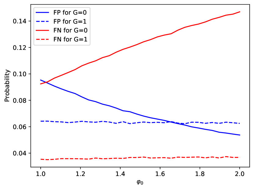
(a) Logit: false positives

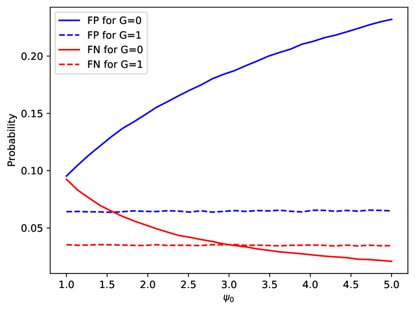
(b) Logit: false negatives

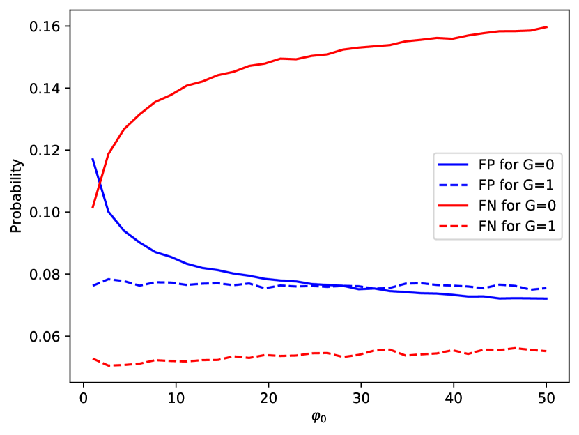
(c) Boosting: false positives

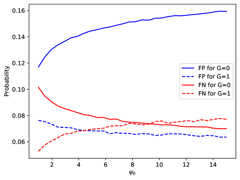
(d) Boosting: false negatives

Figure SM.1: Asymmetric binary choice. The figure shows that introducing asymmetries in the loss function can equalize the False Positive and the False Negative mistakes across groups. Setting: $\rho=0.2$, $\tau=0$, $n=1,000$. Results based on $5,000$ Monte Carlo experiments.

Lastly, we compare the performance of the standard logistic regression approach, which ignores the asymmetric loss function, with the asymmetric logistic regression in terms of the average loss of a social planner. The social planner loss for the former will be denoted by $\ell_{logit}$ while our new estimator yields $\ell_{w-logit}.$

Simulation results are reported in Table SM.2. We report several measures to appraise the findings. First, we report P($\ell_{logit}$ $>$ $\ell_{w-logit}$) which is the percent that the standard logistic regressions generate larger social planner costs compared to our weighted regression. Hence, this measure reports how often our estimator outperforms the standard procedure, where the probabilities are computed from the Monte Carlo simulated samples. Next, we report summary statistics for the ratio $\ell_{logit}/\ell_{w-logit}.$ When the ratio is above 1.00 then the weighted logistic approach is better. We report the minimum, maximum, mean, and three quartiles of the simulation distribution. All simulations involve 5000 replications.

We start from a baseline case for the parameter setting, namely: $\psi_{0}$ = 3, $\psi_{1}$ = 1, $\varphi_{0}$ = 1.7 and finally $\varphi_{1}$ = 1. For the baseline case and $n$ = 1,000, P($\ell_{logit}$ $>$ $\ell_{w-logit}$) is 0.73, meaning that in a large majority of cases our procedure is superior (lower social costs) to the standard logistic regression. According to the summary statistics for the ratio $\ell_{logit}/\ell_{w-logit}$ the mean and median is roughly 1.07/1.06, meaning a 6-7 % reduction in costs, with a max of 1.61 (60% reduction) and a min of 0.74. We also examine various deviations from the baseline case. For the larger sample size $n$ = 5,000 the gains are similar, although with larger values for P($\ell_{logit}$ $>$ $\ell_{w-logit}$), which is now 0.94, meaning that the probability that the symmetric logistic regression leads to larger losses increases as we get more data. Note that the min and max of the distribution move in opposite direction, with the latter now 1.29.

Next we report two columns in Table SM.2 where we change the fraction of protected population from 0.2 to respectively 0.5. These changes do not seem to have a significant impact on any of the results. In contrast, however, if we change the cost structure we see, as might be expected, more variation. More precisely, introducing more asymmetries in the loss function implies better performance of the asymmetric logistic regression.

Lastly, we compare the performance of the weighted ERM decisions to the plug-in rules. Note that in the special case of the symmetric binary classification with the logistic convexification, the plug-in decisions are actually equivalent to the ERM decision since

$$\eta(x)=\frac{1}{1+e^{-f(x)}}>0.5\iff f(x)>0.$$

However, this equivalence does not hold in our asymmetric setting. In addition, some of the popular and successful machine learning techniques, e.g., the support vector machines and neural networks with hinge convexification, are ERM-based and do not estimate $\eta$. For simplicity, we focus on the parametric case and compare the asymmetric Logit to the asymmetric plug-in rules based on the symmetric Logit. These results are presented in Table SM.3. As can be seen, the plug-in rules tend to have higher total costs, which is more pronounced in small samples.

Table SM.1: Monte Carlo Simulation Results: ML Prediction

The Monte Carlo simulation design is presented in Section SM.1, which represents a stylized social planner facing disproportionate number of false positive and false negative mistakes across two groups with the standard ML classification approach. The population consists of two groups, $G$ = 0 and 1. Constituents of group $G$ = 1 are a fraction $\rho.$ Moreover, the dimension $d$ of covariates $Z$ is set to $15$ and the scale parameter is $\sigma=1$. FP and FN are false positive and false negative mistakes computed as a share in the corresponding group, Total = misclassification rate. Logit = logistic regression, GB = Gradient Boosted trees, SL = shallow learning, DL = deep learning, SVM = support vector machines. All results are based on $5,000$ MC experiments.

		Nonlinear DGP: $\tau=1$						Linear DGP: $\tau=0$
		$\rho=0.2$			$\rho=0.5$			$\rho=0.2$			$\rho=0.5$
	G	FP	FN	Error	FP	FN	Error	FP	FN	Error	FP	FN	Error
	Sample size $n$ = 1,000
Logit	0	0.28	0.12	0.37	0.28	0.12	0.33	0.10	0.09	0.17	0.10	0.09	0.14
	1	0.25	0.02		0.25	0.01		0.06	0.04		0.07	0.03
LASSO	0	0.11	0.06	0.16	0.11	0.06	0.14	0.11	0.09	0.19	0.12	0.09	0.16
	1	0.06	0.06		0.08	0.03		0.04	0.11		0.07	0.04
GB	0	0.15	0.09	0.22	0.17	0.08	0.21	0.12	0.10	0.2	0.12	0.10	0.17
	1	0.12	0.06		0.12	0.05		0.08	0.05		0.08	0.04
SVM	0	0.13	0.08	0.2	0.14	0.08	0.18	0.14	0.08	0.2	0.16	0.07	0.17
	1	0.10	0.05		0.10	0.04		0.04	0.11		0.07	0.05
SL	0	0.07	0.03	0.09	0.04	0.06	0.08	0.10	0.08	0.17	0.10	0.08	0.14
	1	0.04	0.02		0.03	0.03		0.07	0.03		0.07	0.03
DL	0	0.06	0.05	0.10	0.06	0.04	0.08	0.10	0.09	0.18	0.28	0.05	0.23
	1	0.04	0.03		0.04	0.03		0.06	0.05		0.10	0.02
	Sample size $n$ = 100
Logit	0	0.25	0.20	0.43	0.25	0.19	0.39	0.14	0.10	0.23	0.17	0.09	0.20
	1	0.19	0.16		0.20	0.13		0.04	0.14		0.06	0.08
LASSO	0	0.23	0.21	0.44	0.26	0.18	0.40	0.17	0.13	0.30	0.22	0.11	0.28
	1	0.14	0.26		0.16	0.20		0.02	0.32		0.06	0.16
GB	0	0.25	0.17	0.41	0.27	0.15	0.37	0.18	0.11	0.29	0.21	0.11	0.24
	1	0.16	0.20		0.18	0.14		0.05	0.22		0.09	0.07
SVM	0	0.30	0.10	0.38	0.33	0.07	0.33	0.21	0.09	0.29	0.29	0.06	0.25
	1	0.19	0.10		0.21	0.06		0.05	0.18		0.08	0.08
SL	0	0.08	0.03	0.10	0.04	0.07	0.09	0.10	0.09	0.17	0.11	0.08	0.14
	1	0.05	0.02		0.03	0.04		0.06	0.03		0.07	0.03
DL	0	0.08	0.04	0.11	0.09	0.03	0.10	0.15	0.06	0.19	0.09	0.11	0.15
	1	0.06	0.02		0.06	0.02		0.08	0.02		0.06	0.04

Table SM.2: Monte Carlo Simulation Results: symmetric vs. asymmetric Logit

The Monte Carlo simulation design is presented in Section SM.1, which represents a stylized social planner with a loss function from Example 2.2 featuring asymmetries for false positives and false negatives. The population consists of two groups, $G$ = 0 and 1, with the former assumed to be a protected segment of the population. Constituents of group $G$ = 1 are a fraction $\rho.$ The baseline case has the loss function with the following setting: $\psi_{1}=\varphi_{1}$ = 1, $\varphi_{0}=1.7$, and $\psi_{0}=3$. We also set $\rho=0.2$, $\sigma=0.3$, and $\tau=0$. We compare the performance of a standard logistic regression approach, which ignores the asymmetric loss function, with our convexified weighted logistic model appearing in equation (SM.1). The social planner loss for the former will be denoted by $\ell_{logit}$ while our new estimator yields $\ell_{w-logit}.$ We report P($\ell_{logit}$ $>$ $\ell_{w-logit}$) which is the percent that standard logistic regressions generate larger social planner costs compared to our weighted regression. Hence, this measure reports how often our estimator outperforms the standard procedure, where the probabilities are computed from the Monte Carlo simulated samples. Next, we report summary statistics for the ratio $\ell_{logit}/\ell_{w-logit}.$ When the ratio is above 1.00 then the weighted logistic approach is better. We report the minimum, maximum, mean, and three quartiles of the simulation distribution. Columns with $\varphi_{0},\varphi_{1},\psi_{0}$, or $\psi_{1}$ as headers represent deviations from the baseline case.

	Baseline	$\rho$	$\tau$	$\varphi_{0}$	$\varphi_{1}$	$\varphi_{1}$	$\psi_{0}$	$\psi_{1}$	$\psi_{1}$
	case	0.5	1	2	2	3	4	2	3
	Sample size $n$ = 1,000
P($\ell_{logit}$ $>$ $\ell_{w-logit}$)	0.57	0.46	0.93	0.5	0.69	0.76	0.67	0.68	0.75
Summary statistics for $\ell_{plugin}/\ell_{w-logit}$
Mean	1.05	1.02	1.15	1.02	1.09	1.14	1.11	1.09	1.14
Min	0.58	0.33	0.85	0.56	0.48	0.43	0.50	0.41	0.53
1st Quantile	0.94	0.91	1.07	0.94	0.97	1.00	0.96	0.97	1.00
Median	1.03	1.00	1.14	1.00	1.07	1.12	1.08	1.07	1.12
3rd Quantile	1.14	1.10	1.21	1.09	1.19	1.25	1.23	1.19	1.25
Max	2.11	2.21	1.63	1.93	2.22	2.69	2.66	2.33	2.69
	Sample size $n$ = 5,000
P($\ell_{logit}$ $>$ $\ell_{w-logit}$)	0.76	0.67	0.99	0.62	0.80	0.86	0.91	0.81	0.85
Summary statistics for $\ell_{logit}/\ell_{w-logit}$
Mean	1.06	1.04	1.10	1.02	1.07	1.09	1.14	1.07	1.09
Min	0.81	0.79	0.95	0.83	0.79	0.81	0.81	0.81	0.85
1st Quantile	1.00	0.98	1.06	0.98	1.01	1.03	1.06	1.02	1.03
Median	1.05	1.04	1.10	1.02	1.07	1.09	1.13	1.07	1.09
3rd Quantile	1.11	1.09	1.13	1.06	1.12	1.15	1.21	1.12	1.15
Max	1.36	1.41	1.29	1.30	1.43	1.48	1.61	1.48	1.46

Table SM.3: Monte Carlo Simulation Results: plug-in vs. asymmetric Logit

The Monte Carlo simulation design is presented in Section SM.1, which represents a stylized social planner with a loss function from Example 2.2 featuring asymmetries for false positives and false negatives. The population consists of two groups, $G$ = 0 and 1, with the former assumed to be a protected segment of the population. Constituents of group $G$ = 1 are a fraction $\rho.$ The baseline case has the loss function with the following setting: $\psi_{1}=\varphi_{1}$ = 1, $\varphi_{0}=1.7$, and $\psi_{0}=3$. We also set $\rho=0.2$, $\sigma=0.3$, and $\tau=0$. We compare the performance of a standard logistic regression approach, which ignores the asymmetric loss function, with our convexified weighted logistic model appearing in equation (SM.1). The social planner loss for the former will be denoted by $\ell_{plugin}$ while our new estimator yields $\ell_{w-logit}.$ We report P($\ell_{plugin}$ $>$ $\ell_{w-logit}$) which is the percent that standard logistic regressions generate larger social planner costs compared to our weighted regression. Hence, this measure reports how often our estimator outperforms the standard procedure, where the probabilities are computed from the Monte Carlo simulated samples. Next, we report summary statistics for the ratio $\ell_{plugin}/\ell_{w-logit}.$ When the ratio is above 1.00 then the weighted logistic approach is better. We report the minimum, maximum, mean, and three quartiles of the simulation distribution. Columns with $\varphi_{0},\varphi_{1},\psi_{0}$, or $\psi_{1}$ as headers represent deviations from the baseline case.

	Baseline	$\rho$	$\tau$	$\varphi_{0}$	$\varphi_{1}$	$\varphi_{1}$	$\psi_{0}$	$\psi_{1}$	$\psi_{1}$
	case	0.5	1	2	2	3	4	2	3
	Sample size $n$ = 1,000
P($\ell_{plugin}$ $>$ $\ell_{w-logit}$)	0.67	0.67	0.48	0.59	0.66	0.64	0.69	0.65	0.66
Summary statistics for $\ell_{plugin}/\ell_{w-logit}$
Mean	1.08	1.10	1.00	1.05	1.07	1.06	1.11	1.07	1.07
Min	0.48	0.42	0.88	0.48	0.57	0.58	0.49	0.50	0.47
1st Quantile	0.96	0.96	0.99	0.95	0.96	0.95	0.97	0.96	0.96
Median	1.07	1.08	1.00	1.04	1.06	1.05	1.09	1.06	1.06
3rd Quantile	1.18	1.22	1.02	1.14	1.16	1.16	1.23	1.16	1.17
Max	1.98	2.84	1.09	1.93	2.17	2.05	2.34	2.11	1.98
	Sample size $n$ = 5,000
P($\ell_{plugin}$ $>$ $\ell_{w-logit}$)	0.55	0.56	0.66	0.52	0.54	0.53	0.57	0.53	0.54
Summary statistics for $\ell_{plugin}/\ell_{w-logit}$
Mean	1.01	1.01	1.00	1.00	1.00	1.00	1.01	1.00	1.01
Min	0.81	0.81	0.97	0.87	0.83	0.82	0.81	0.83	0.85
1st Quantile	0.97	0.97	1.00	0.98	0.97	0.98	0.97	0.97	0.98
Median	1.01	1.01	1.00	1.01	1.01	1.00	1.01	1.00	1.01
3rd Quantile	1.04	1.05	1.01	1.03	1.04	1.03	1.05	1.03	1.03
Max	1.18	1.24	1.03	1.23	1.18	1.19	1.32	1.22	1.20

SM.2 Pretrial detention costs and benefits

In this section we provide a summary of the cost benefit analysis reported by Baughman (2017) to build a preference-based approach for the empirical application appearing in Section 5. In Table SM.6 we provide the key elements of the aforementioned study, which will serve as inputs to the $EBD(c_{i}),$ $ECD(d_{i})$ and $C(x_{i},c_{i})$ appearing in equation (5). In particular, based on Table SM.6 we define:

$$EBD(c_{i})=\sum_{crimetype}\mathbbm{1}_{crimetype=c_{i}}EBD_{crimetype}$$

where $EBD_{crimetype}$ is obtained from averaging the entries to Panel B in Table SM.6 (and dividing by 1000) and adding the entries of Panel C. These entries are summarized in Table SM.5. The function is scaled by 0.05 to balance the costs.

Table SM.4: Summary Statistics Data

Summary statistics of recidivism data set from Broward County, Florida originally compiled by ProPublica (see Larson et al. (2016)). We use an excerpt of the original data, considering only black and white defendants who were assigned COMPAS risk scores within 30 days of their arrest, were not arrested for an ordinary traffic offense, and defendants who spent at least two years (after their COMPAS evaluation) outside a correctional facility without being arrested for a violent crime, or were arrested for a violent crime within this two-year period. The entry $is\_recid$ pertains to the binary outcome of recidivism, Decile Score refers to the COMPAS score.

Gender	Male	Female
	8972	2209
is_recid	0	1
	7486	3695
Race	African	Asian	Caucasian	Hispanic	Native
	American				American	Other
	5751	52	3822	910	30	616
Crime	Aggravated	Arson	Fraud	Household	Larceny
	Assault			Burglary	Theft
	2771	6275	224	577	1028
	Rape	Robbery	Murder	Motor Vehicle
	Sexual Assault			Theft
	38	82	9	177
	Min.	25% Quantile	Median	Mean	75% Quantile	Max
Decile Score	-1	2	4	4.577	7	10
Prior crime count	0	0	1	3.263	4	38
Age	18	25	31	34.33	42	96
Detention Days	0	0	1	21.69	8	2152

Table SM.5: Economic costs and benefits - Summary entries for EBD and ECD functions

$crimetype$	$C_{crimetype}$		$EBD_{crimetype}$
Murder	10,754		11,732
Rape/Sexual Assault	266		353
Aggravated Assault	126		127
Robbery	48		230
Arson/Other	23		292
Motor Vehicle Theft	11		53
Household Burglary	7		64
Forgery/Counterfeiting	5		46
Fraud	5		49
Larceny/Theft	3		43

The function $C(x_{i},C_{i})$ is computed as the median of future recidivism costs, which is 23. Finally, from Panel D in Table SM.6 we calculate $ECD(d_{i}),$ using both individual and public costs, again scaling by 1000. Namely (assuming $m_{i}$ = 30$d_{i}$), which yields $0.347d_{i}$ namely:

$$\text{ECD}(d_{i}) = \underbrace{\frac{1}{1000}\times\left[\frac{1036+590}{90}+\frac{1565}{30}\right]}d_{i}+$$

Individual Costs I

$$\underbrace{\frac{1}{1000}\times\left[\frac{31028+1938+103670*(.17)+136191*(.032)}{365}\right]}d_{i}+$$

Individual Costs II

$$\underbrace{\frac{1}{1000}\times\left[\frac{31406+5142+1249+8293}{365}\right]}d_{i}$$

Public Costs

$$= 0.347d_{i}$$

Table SM.6: Economic costs and benefits

This table uses inputs from Baughman (2017) Tables 1 through 3 to construct the costs and benefits used in our empirical applications.

	Panel A:	Panel B:
	Total Per-Offense Cost	Economic Benefits
	for Different Crimes ($)	of Detention ($)
Type of Offense		Low Estimate	High Estimate
Murder	10,754,332	4,602,326	18,780,120
Rape/Sexual Assault	266,332	136,191	488,243
Aggravated Assault	126,585	14,715	158,250
Robbery	48,589	12,523	364,898
Arson/Other	23,839	75,453	426,571
Motor Vehicle Theft	11,936	5949	19,299
Household Burglary	7175	2192	44,875
Forgery/Counterfeiting	5821	5731	10,439
Fraud	5563	3950	5478
Larceny/Theft	3906	580	3839
Panel C: Benefit Categories
Avoidance of Felony for Which
No Arrest Is Made			40,338
Avoidance of Failure to Appear			518
Panel D: Economic Costs of Detention
Individual Costs per individual
Loss of Freedom	$(\$1036/90)d_{i}$
Loss of Income	$(\$31,028/365)d_{i}$
Loss of Housing	$\$1565m_{i}$
Childcare Costs	$(\$1938/365)d_{i}$
Stolen or Lost Property	$(\$590/3)m_{i}$
Strain on Intimate Relationships	$(\$103,670(.17)/365)d_{i}$
Possibility of Violent or Sexual Assault	$(\$136,191(.032)/365)d_{i}$
Public Costs
Prison Operation Costs	$(\$31,406/365)d_{i}$
Loss of Federal Tax	$(5142/365)d_{i}$
Loss of State Tax	$(\$1249/365)d_{i}$
Welfare for Detainee’s Family	$(\$8293/365)d_{i}$

SM.3 Empirical results

We consider the following empirical model specifications: (1) logistic regression covered in Section 4.1, (2) shallow and deep learning in Sections 4.2 and Section SM.4, and (3) boosting covered in Section C. In each case we compare symmetric versus asymmetric costs, with the latter involving two costs schemes. In all specifications we use as dependent variable a dummy of Recidivism occurrence. The explanatory variables are: (a) race as a categorical variable, (b) gender using female indicator, (c) crime history: prior count of crimes, (d) COMPASS score, (e) crime factor: whether crime is felony or not and (e) interaction between race factor and compass score.

The results are reported in Table SM.7 compliment those in the main paper. We report respectively: (a) True & False Positive/Negative Costs, (b) overall cost, (c) True & Positives/Negatives, (d) True/False Positive Rates, (e) area under the ROC curve (AUC) during the training and testing sample. For each estimation procedure we compare side-by-side the unweighted, i.e. traditional symmetric, and weighted procedure.

The Boosting model yields results that are worse, both in terms of weighted versus unweighted and vis-à-vis the logistic regression, although the AUC results are overall better than for the logistic regression.

Table SM.7: Empirical Results

Empirical results with (1) logistic regression covered in Section 4.1, (2) shallow and deep learning in Section 4.2 and Online Appendix Section SM.4, and (3) boosting covered in Section C. The setting involves two groups with cost structure appearing in Table 1.

	Logit		Boosting
	Unweighted	Weighted	Unweighted	Weighted
True Positive Cost	-1310	-2150	-1674	-2332
False Negative Cost	5575	4771	5141	4085
True Negative Cost	0	0	0	0
False Positive Cost	2415	3289	3036	3680
Overall cost	6680	5909	6503	5433
TP	178	206	228	228
FN	577	549	527	527
TN	1438	1400	1411	1383
FP	105	143	132	160
TP Rate	0.24	0.27	0.30	0.30
FP Rate	0.07	0.09	0.09	0.10
AUC_train	0.69	0.67	0.73	0.71
AUC_test	0.69	0.67	0.7	0.68
	No Hidden Layer
	Hinge Convexification		Logistic Convexification
	Unweighted	Weighted	Unweighted	Weighted
True Positive Cost	-1930	-2360	-1310	-2150
False Negative Cost	4395	3971	5575	4771
True Negative Cost	0	0	0	0
False Positive Cost	4646	4186	2415	3289
Overall cost	7111	5797	6680	5909
TP	247	251	178	206
FN	508	504	577	549
TN	1341	1361	1438	1400
FP	202	182	105	143
TP Rate	0.33	0.33	0.24	0.27
FP Rate	0.13	0.12	0.07	0.09
AUC_train	0.7	0.69	0.69	0.67
AUC_test	0.69	0.68	0.69	0.67

Table SM.7 continued

	Shallow Learning - One Hidden Layer
	Deep Learning: Two Hidden Layers
	Hinge Convexification		Logistic Convexification
	Unweighted	Weighted	Unweighted	Weighted
True Positive Cost	-1677	-2266	-2045	-2149
False Negative Cost	5288	4488	5232	4763
True Negative Cost	0	0	0	0
False Positive Cost	2645	3220	3335	3381
Overall cost	6256	5442	6521	5994
TP	202	236	229	203
FN	553	519	526	552
TN	1428	1403	1398	1396
FP	115	140	145	147
TP Rate	0.27	0.31	0.3	0.27
FP Rate	0.07	0.09	0.09	0.1
AUC_train	0.64	0.62	0.7	0.69
AUC_test	0.65	0.64	0.7	0.68
	Deep Learning: Three Hidden Layers
	Hinge Convexification		Logistic Convexification
	Unweighted	Weighted	Unweighted	Weighted
True Positive Cost	-1774	-2379	-2272	-2500
False Negative Cost	5495	4652	5642	4967
True Negative Cost	0	0	0	0
False Positive Cost	2530	3220	3427	3864
Overall cost	6251	5493	6796	6331
TP	192	235	234	217
FN	563	520	521	538
TN	1433	1403	1394	1375
FP	110	140	149	168
TP Rate	0.25	0.31	0.31	0.29
FP Rate	0.07	0.09	0.1	0.11
AUC_train	0.64	0.62	0.71	0.69
AUC_test	0.65	0.62	0.7	0.68

SM.4 Shallow learning

The shallow learning amounts to fitting a neural network with one or two hidden layers. Neural networks are widely used in econometrics at least since Gallant and White (1988). We focus on a very simple neural network class consisting of two hidden layers. Following the recent trends in big data applications, we refer to this approach shallow learning which in contrast to the deep learning does not allow for the number of layers to scale with the sample size. Consider a single layer neural network class

$$\Theta_{n}^{\rm S}=\left\{x\mapsto\sum_{j=1}^{p_{n}}b_{j}\sigma_{0}(a_{j}^{\top}x+a_{0})+b_{0},\quad a\in\mathbf{R}^{d+1},\;|b|_{1}\leq\gamma_{n}\right\},$$

where $a=(a_{0},a_{1},\dots,a_{d})$ and $b=(b_{0},b_{1},\dots,b_{p_{n}})$ are parameters to be estimated, $\sigma_{0}$ is some smooth function, and $|.|_{1}$ is the $\ell_{1}$ norm. Our shallow learning class is defined as a hybrid network

$$\mathscr{F}_{n}^{S}=\left\{x\mapsto\sigma(\theta(x)+c(x)d+1)-\sigma(\theta(x)+c(x)d-1)-1:\;\theta\in\Theta_{n}^{\rm S},\;|d|\leq n\right\},$$

where $c(x)$ pertains to asymmetry (see equation (3.2)) and $\sigma(z)=(z)_{+}$ is the Rectified Linear Unit (ReLU) activation function. The shallow learning class can be visualized on a directed graph, see Figure SM.2. All covariates are fed first into the hidden layer 1 corresponding to $\Theta_{n}^{\rm S}$. This network class consists of $p_{n}$ neurons with a smooth activation function $\sigma_{0}$. The output produced by the hidden layer 1 is fed subsequently into the two neurons with the ReLU activation function $\sigma$. Note that this last layer has a single free parameter $b$. The output $f\in[-1,1]$, is obtained from summing up the two neurons from the ReLU layer. The final binary decision is $\mathrm{sign}(f)$.

Figure SM.2: Directed graph of the shallow learning architecture with $d=3$ covariates, single hidden layer with $4$ neurons, and 2 outer ReLU neurons. The yellow neuron takes covariates $X\in\mathbf{R}^{d}$ as an input and produces $c(X)\in\mathbf{R}$, which is fed directly in 2 ReLU neurons.

The soft shallow learning prediction $\hat{f}_{n}:\mathcal{X}\to[-1,1]$ is a solution to the convexified empirical risk minimization problem with hinge convexifying function

$$\inf_{f\in\mathscr{F}_{n}^{\rm S}}\frac{1}{n}\sum_{i=1}^{n}\omega(Y_{i},X_{i})(1-Y_{i}f(X_{i}))_{+}.$$

To describe the accuracy of the shallow learning binary decision $\mathrm{sign}(\hat{f}_{n})$, consider the Sobolev ball of smoothness $\beta\in\mathbf{N}$ and radius $M\in(0,\infty)$

$$W^{\beta,\infty}_{M}(\mathcal{X})=\left\{f:\mathcal{X}\to\mathbf{R}:\;\max_{|k|\leq\beta}\mathrm{esssup}_{x\in\mathcal{X}}|D^{k}f(x)|\leq M\right\},$$

where we use the multi-index notation $k=(k_{1},\dots,k_{d})\in\mathbf{N}^{d}$, $|k|=k_{1}+\dots+k_{d}$, and $D^{k}f=\frac{\partial^{|k|}}{\partial x_{1}^{k_{1}}\dots\partial x_{d}^{k_{d}}}f$.

The following assumption imposes some mild regularity conditions on the activation function $\sigma_{0}$ and the Sobolev smoothness of the conditional probability $\eta$.

Assumption SM.4.1.

(i) $\sigma_{0}:\mathbf{R}\to[-b,b]$ is non-decreasing and Lipschitz continuous, infinitely differentiable on some open interval containing some $x_{0}$ with $D^{k}\sigma_{0}(x_{0})\neq 0$ for all $k\in\mathbf{Z}_{+}$; (ii) $\eta\in W^{\beta,\infty}_{M}(\mathcal{X})$ for some $\beta\in\mathbf{N}$ and $0<M<\infty$, where $\mathcal{X}\subset\mathbf{R}^{d}$ is a Cartesian product of compact intervals; (iii) $p_{n}$ and $\gamma_{n}$ are of polynomial order.

Assumption SM.4.1 (i) rules out polynomial activation functions and allows for the sigmoid function $\sigma_{0}(x)=(1+e^{-x})^{-1}$. It also rules out the ReLU activation function, which is a more natural choice for the deep learning problems and is considered in the subsequent section.

Theorem SM.1.

Suppose that $(Y_{i},X_{i})_{i=1}^{n}$ is an i.i.d. sample following a distributions satisfying Assumptions 3.1, 3.2, 3.3, and SM.4.1, and denoted $\mathcal{P}(\alpha,\beta)$. Then there exist $c,C>0$ such that for every $t>0$ with probability at least $1-ce^{-t}$

$$\mathcal{R}(\mathrm{sign}(\hat{f}_{n}))-\mathcal{R}^{*}\leq C\left[\left(\frac{p_{n}\log^{2}n}{n}\right)^{\frac{1+\alpha}{2+\alpha}}+p_{n}^{-(1+\alpha)\beta/d}+\left(\frac{t}{n}\right)^{\frac{1+\alpha}{2+\alpha}}+\frac{t}{n}\right]$$

uniformly over $\mathcal{P}(\alpha,\beta)$. In particular,

$$\sup_{P\in\mathcal{P}(\alpha,\beta)}\mathbb{E}_{P}\left[\mathcal{R}(\mathrm{sign}(\hat{f}_{n}))-\mathcal{R}^{*}\right]\lesssim\left(\frac{\log^{2}n}{n}\right)^{\frac{(1+\alpha)\beta}{(2+\alpha)\beta+d}}$$

provided that $p_{n}\sim(n/\log^{2}n)^{\frac{d}{(2+\alpha)\beta+d}}$.

It is worth noting that the convergence rate of the excess risk of the shallow learning prediction can be anywhere between the slow nonparametric rate $O(n^{-\beta/(2\beta+d)})$ and the fast rate $O(n^{-1})$ depending on the margin exponent $\alpha$. In particular, we can partially offset the curse of dimensionality if $\alpha$ is sufficiently large, e.g., for $\alpha=d/\beta$, the rate is $O(n^{-1/2})$. This is another manifestation of the fact that predicting a binary outcome is easier than predicting real-valued variables. Note also that the smoothness of the decision boundary itself $\{x\in[0,1]^{d}:\;\eta(x)-c(x)=0\}$ does not directly play a role and only the smoothness of $\eta$ is important. This is probably not surprising in light of the fact that $c$ is known to the decision maker.

In the special case when the loss function is symmetric, under the mild assumption that the density of covariates is uniformly bounded, it follows from Audibert and Tsybakov (2007), Theorem 4.1 that there exists $C>0$ such that for every $n\geq 1$

$$\inf_{\hat{f}_{n}}\sup_{P\in\mathcal{P}(\alpha,\beta)}\mathbb{E}_{P}\left[\mathcal{R}(\hat{f}_{n})-\mathcal{R}^{*}\right]\geq Cn^{-\frac{(1+\alpha)\beta}{(2+\alpha)\beta+d}},$$ (SM.2)

where the infimum is taken over all binary decisions $\hat{f}_{n}:\mathcal{X}\to\{-1,1\}$ computed from an i.i.d. sample $(Y_{i},X_{i})_{i=1}^{n}$. Therefore, apart for a $\log n$ factor, our result shows that binary decisions produced by the shallow learning are optimal from the minimax point of view.

Proof of Theorem SM.1.

By Theorem 4.1, for every $t>0$ with probability at least $1-c_{q}e^{-t}$

$$\mathcal{R}(\mathrm{sign}(\hat{f}_{n}))-\mathcal{R}^{*}\lesssim\psi_{n,1+1/\alpha}^{\sharp}(\epsilon)+\left(\frac{t}{n}\right)^{\frac{1+\alpha}{2+\alpha}}+\frac{t}{n}+\inf_{f\in\mathscr{F}_{n}^{\rm S}}{\mathcal{R}}_{\phi}(f)-\mathcal{R}_{\phi}^{*},$$

where we use the fact that $\gamma=1$ and $\kappa=1+1/\alpha$ by Lemmas B.4 and B.9. By Lemmas SM.5.1 and SM.5.3

$$\psi_{n,1+1/\alpha}^{\sharp}(\epsilon)\leq C\left(\frac{p_{n}\log p_{n}}{n}\log\left(\frac{n}{p_{n}\log p_{n}}\right)\right)^{\frac{1+\alpha}{2+\alpha}}.$$

Next, under Assumption SM.4.1 (ii), by Mhaskar (1996), Theorem 2.1, there exists $\eta_{n}\in\Theta_{n}^{\rm S}$ such that

$$\|\eta_{n}-\eta\|_{\infty}\leq Cp_{n}^{-\beta/d}\triangleq\varepsilon_{n}.$$

Define

$$f_{n}(x)=\left(\frac{\eta_{n}(x)-c(x)}{\varepsilon_{n}}+1\right)_{+}-\left(\frac{\eta_{n}(x)-c(x)}{\varepsilon_{n}}-1\right)_{+}-1$$

and note that $f_{n}\in\mathscr{F}_{n}^{\rm S}$. Note also that

$$f_{n}(x)=\begin{cases}1,&\text{if }\eta_{n}(x)-c(x)>\varepsilon_{n}\\ \frac{\eta_{n}(x)-c(x)}{\varepsilon_{n}},&\text{if }|\eta_{n}(x)-c(x)|\leq\varepsilon_{n}\\ -1,&\text{if }\eta_{n}(x)-c(x)<-\varepsilon_{n}\end{cases}$$

and that on the event $\{x\in[0,1]^{d}:\;|\eta(x)-c(x)|>2\varepsilon_{n}\}$ we have $f_{n}=f_{\phi}^{*}$. To see this, recall that by Lemma B.4, $f_{\phi}^{*}=\mathrm{sign}(\eta-c)$. Then if $\eta-c>0$, we have $\eta_{n}-c=(\eta-c)-(\eta-\eta_{n})>\varepsilon_{n}$ while if $\eta-c<0$, we have $\eta_{n}-c=(\eta-c)+(\eta_{n}-\eta)<-\varepsilon_{n}$. Therefore, by Lemma B.8

$$\inf_{f\in\mathscr{F}_{n}^{\rm S}}{\mathcal{R}}_{\phi}(f)-\mathcal{R}_{\phi}^{*} =\inf_{f\in\mathscr{F}_{n}^{\rm S}}\int_{[0,1]^{d}}b|f-f_{\phi}^{*}||\eta-c|\mathrm{d}P_{X}$$

$$\leq\int_{[0,1]^{d}}b|f_{n}-f_{\phi}^{*}||\eta-c|\mathrm{d}P_{X}$$

$$=\int_{|\eta-c|\leq 2\varepsilon_{n}}b|f_{n}-f_{\phi}^{*}||\eta-c|\mathrm{d}P_{X}$$

$$\leq 8M\varepsilon_{n}\int_{|\eta-c|\leq 2\varepsilon_{n}}b|f_{n}-f_{\phi}^{*}|\mathrm{d}P_{X}$$

$$\leq 16M\varepsilon_{n}P_{X}(|\eta-c|\leq 2\varepsilon_{n})$$

$$\leq 2^{4+\alpha}MC_{m}\varepsilon_{n}^{1+\alpha},$$

where the last two lines follow under Assumptions 3.1 (iii) and 3.3. Therefore, for every $t>0$ with probability at least $1-c_{q}e^{-t}$

$$\mathcal{R}(\mathrm{sign}(\hat{f}_{n}))-\mathcal{R}^{*} \lesssim\left(\frac{p_{n}\log^{2}n}{n}\right)^{\frac{1+\alpha}{2+\alpha}}+p_{n}^{-(1+\alpha)\beta/d}+2^{4+\alpha}MC_{m}C^{1+\alpha}\left(\frac{t}{n}\right)^{\frac{1+\alpha}{2+\alpha}}+\frac{t}{n}.$$

The second statement follows from integrating this tail bound in the same way as in the proof of Theorem 4.2. The uniformity follows from the fact that all constants do no depend on the specific distribution of $(X,Y)$ in $\mathcal{P}(\alpha,\beta)$. ∎

SM.5 Fixed points of local Rademacher complexities

In this section, we obtain useful bounds on fixed points of local Rademacher complexities for shallow and deep neural network classes.

Next, we consider the shallow learning class

$$\mathscr{F}_{n}^{\rm S}=\left\{\sigma(\theta+cd+1)-\sigma(\theta+cd-1)-1:\;\theta\in\Theta_{n}^{\rm S},\;|d|\leq n\right\},$$

where $\sigma(z)=\max\{z,0\}$,

$$\Theta_{n}^{\rm S}=\left\{x\mapsto\sum_{j=1}^{p_{n}}b_{j}\sigma_{0}(a_{j}^{\top}x+a_{0,j})+b_{0},\quad a_{j}\in\mathbf{R}^{d},\quad\sum_{j=0}^{p_{n}}|b_{j}|\leq\gamma_{n}\right\},$$

The following result bounds the local Rademacher complexity of the shallow learning class $\mathscr{F}_{n}^{\rm S}$ in terms of the number of neurons $p_{n}$ in the inner neural network class $\Theta_{n}^{\rm S}$.

Lemma SM.5.1.

Suppose that (i) $\sigma_{0}:\mathbf{R}\to[-b,b]$ is non-decreasing with Lipschitz constant $L_{0}<\infty$; (ii) $p_{n}=C_{1}n^{c_{1}}$ and $\gamma_{n}=C_{2}n^{c_{2}}$ for some constants $c_{j},C_{j}>0,j=1,2$; (iii) $\|c\|_{\infty}\leq\bar{c}$ and $\gamma_{n}>2/L_{0}$. Then for $a,A,K>0$,

$$\psi_{n}(\delta;\mathscr{F}_{n}^{\rm S})\leq K\left[\sqrt{\frac{p_{n}\delta(1\vee\log(An^{a}/\delta^{1/2}))}{n}}\bigvee\frac{p_{n}(1\vee\log(An^{a}/\delta^{1/2}))}{n}\right].$$

Proof.

Put

$$\mathscr{F}_{n}(\delta)\triangleq\left\{f-f_{n}^{*}:\;f\in\mathscr{F}_{n}^{\rm S},\;\|f-f^{*}_{n}\|\leq\sqrt{\delta}\right\}$$

and $\sigma^{2}_{n}\triangleq\sup_{g\in\mathscr{F}_{n}(\delta)}P_{n}g^{2}$. By Dudley’s entropy bound, see Koltchinskii (2011), Theorem 3.11, for some numerical constant $C_{0}$

$$\psi_{n}(\delta;\mathscr{F}_{n}^{\rm S}) =\mathbb{E}\left[\sup_{g\in\mathscr{F}_{n}(\delta)}|R_{n}g|\right]$$ (SM.3)

$$\leq\frac{C_{0}}{\sqrt{n}}\mathbb{E}\int_{0}^{2\sigma_{n}}\sqrt{\log N(\mathscr{F}_{n}(\delta),L_{2}(P_{n}),\varepsilon)}\mathrm{d}\varepsilon$$

and by the symmetrization and contraction inequalities, see Koltchinskii (2011), Theorems 2.1 and 2.3

$$\mathbb{E}\sigma^{2}_{n} \leq\mathbb{E}\left[\sup_{g\in\mathscr{F}_{n}(\delta)}\left|(P_{n}-P)g^{2}\right|\right]+\sup_{g\in\mathscr{F}_{n}(\delta)}Pg^{2}$$

$$\leq 2\mathbb{E}\left[\sup_{g\in\mathscr{F}_{n}(\delta)}|R_{n}g^{2}|\right]+\delta$$

$$\leq 16\psi_{n}(\delta;\mathscr{F}_{n}^{\rm S})+\delta$$

$$\triangleq B,$$

where the third line follows since $\|f\|_{\infty}\leq 1,\forall f\in\mathscr{F}_{n}^{\rm S}$. Next, for a sequence $x=(x_{1},\dots,x_{n})\in\mathcal{X}^{n}$ and a class of functions from $\mathcal{X}$ to $\mathbf{R}$, denoted $\mathscr{F}$, we consider the class $\mathscr{F}|_{x}\triangleq\left\{(f(x_{1}),f(x_{2}),\dots,f(x_{n})):\;f\in\mathscr{F}\right\}\subset\mathbf{R}^{n}$. For $\varepsilon>0$, let $N(\mathscr{F}|_{x},\ell_{\infty},\varepsilon)$ be the $\varepsilon$-covering number of $\mathscr{F}|_{x}$ with respect to the $\ell_{\infty}$ distance. The uniform covering number is defined as

$$N_{\infty}(\mathscr{F}_{n}(\delta),n,\varepsilon)\triangleq\max\{N(\mathscr{F}_{n}(\delta)|_{x},\ell_{\infty},\varepsilon):\;x\in\mathcal{X}^{n}\}.$$

By Anthony and Bartlett (2009), Lemma 10.5, we can bound the $L_{2}(P_{n})$ covering numbers as follows

$$N(\mathscr{F}_{n}(\delta),L_{2}(P_{n}),\varepsilon) =N(\mathscr{F}_{n}(\delta)|_{X_{1},\dots,X_{n}},\ell_{2},\varepsilon)$$

$$\leq\max\{N(\mathscr{F}_{n}^{\rm S}|_{x},\ell_{2},\varepsilon):\;x\in\mathcal{X}^{n}\}$$

$$\leq N_{\infty}(\mathscr{F}_{n}^{\rm S},n,\varepsilon)$$

Note that for $f_{1},f_{2}\in\mathscr{F}_{n}^{\rm S}$, we have $f_{j}(x)=\sigma(\theta_{j}(x)+c(x)d_{j}+1)-\sigma(\theta_{j}(x)+c(x)d_{j}-1)-1$ for some $\theta_{j}\in\Theta_{n}^{\rm S}$ and $|d_{j}|\leq n$ with $j=1,2$. Since $x\mapsto\sigma(x+1)-\sigma(x-1)-1$ is Lipschitz continuous with Lipschitz constant $1$

$$\max_{1\leq i\leq n}|f_{1}(X_{i})-f_{2}(X_{i})|\leq\max_{1\leq i\leq n}|\theta_{1}(X_{i})-\theta_{2}(X_{i})|+\|c\|_{\infty}|d_{1}-d_{2}|$$

Since the $\varepsilon$-covering number of $[-n,n]$ is $n/\varepsilon$,

$$N_{\infty}(\mathscr{F}_{n}^{\rm S},n,\varepsilon) \leq\frac{2\bar{c}n}{\varepsilon}N_{\infty}(\Theta_{n}^{\rm S},n,\varepsilon/2)$$

$$\leq\frac{2\bar{c}n}{\varepsilon}\left(\frac{8ebn[(d+1)p_{n}+1](L_{0}\gamma_{n})^{2}}{\varepsilon(L_{0}\gamma_{n}-1)}\right)^{(d+1)p_{n}+1}$$

$$\leq\frac{2\bar{c}n}{\varepsilon}\left(\frac{16eb(d+2)L_{0}np_{n}\gamma_{n}}{\varepsilon}\right)^{(d+1)p_{n}+1},$$

where the second inequality follows by Anthony and Bartlett (2009), Theorem 14.5 for all $\varepsilon\leq 4b\wedge 2\bar{c}/e$; the third since $(L_{0}\gamma_{n})^{2}/(L_{0}\gamma_{n}-1)\leq 2L_{0}\gamma_{n}$ under (iii). In conjunction with the inequality (SM.3), this shows that

$$\psi_{n}(\delta;\mathscr{F}_{n}^{\rm S}) \leq\frac{C_{0}}{\sqrt{n}}\mathbb{E}\int_{0}^{2\sigma_{n}}\sqrt{\log(2\bar{c}n/\varepsilon)+[(d+1)p_{n}+1]\log(16ebL_{0}(d+2)np_{n}\gamma_{n}/\varepsilon)}\mathrm{d}\varepsilon$$

$$\leq C_{0}\sqrt{\frac{2(d+1)p_{n}}{n}}\mathbb{E}\int_{0}^{2\sigma_{n}}\sqrt{\log((2\bar{c})\vee(16ebL_{0}(d+2)p_{n}\gamma_{n})n/\varepsilon)}\mathrm{d}\varepsilon.$$

Note that for $A>0$

$$\mathbb{E}\int_{0}^{2\sigma_{n}}\sqrt{\log(A/\varepsilon)}\mathrm{d}\varepsilon \leq\int_{0}^{2\sqrt{\mathbb{E}\sigma^{2}_{n}}}\sqrt{\log(A/\varepsilon)}\mathrm{d}\varepsilon$$

$$\leq A\int_{0}^{2\sqrt{B}/A}\sqrt{\log(1/u)}\mathrm{d}u$$

$$\leq 4\sqrt{B}\left\{1\vee\sqrt{\log(A/2\sqrt{\delta})}\right\},$$

where the first line follows by Jensen’s inequality since $t\mapsto\int_{0}^{t}h(u)\mathrm{d}u$ is concave whenever $h$ is non-decreasing; and the last since $\delta\leq B$.

Therefore,

$$\psi_{n}(\delta;\mathscr{F}_{n}^{\rm S})\leq C\sqrt{\frac{p_{n}}{n}\left\{1\vee\log(An^{a}/\delta^{1/2})\right\}}\left(4\sqrt{\psi_{n}(\delta;\mathscr{F}_{n}^{\rm S})}+\sqrt{\delta}\right),$$

with $C=4C_{0}\sqrt{2(d+1)}$, $A=\bar{c}\vee(8ebL_{0}(d+2)C_{1}C_{2})$, and $a=c_{1}+c_{2}+1$. Solving this inequality for $\psi_{n}(\delta;\mathscr{F}_{n}^{\rm S})$ gives

$$\psi_{n}(\delta;\mathscr{F}_{n}^{\rm S})\leq 8C(4C\vee 1)\left[\sqrt{\frac{p_{n}\delta\{1\vee\log(An^{a}/\delta^{1/2})\}}{n}}\bigvee\frac{p_{n}\{1\vee\log(An^{a}/\delta^{1/2})\}}{n}\right].$$

∎

Next, we consider the deep learning class

$$\mathscr{F}_{n}^{\rm DNN} =\left\{\sigma(\theta+cd+1)-\sigma(\theta+cd-1)-1:\;|d|\leq n,\;\theta\in\Theta_{n}^{\rm DNN}\right\},$$

where

$$\Theta_{n}^{\rm DNN}=\left\{f(x)=A_{L}\sigma_{\mathbf{b}_{L}}\circ A_{L-1}\sigma_{\mathbf{b}_{L-1}}\circ\dots\circ A_{1}\sigma_{\mathbf{b}_{1}}\circ A_{0}x,\;\|f\|_{\infty}\leq F\right\}$$

is a deep neural network class such that $\{A_{l},\mathbf{b}_{l}:\;1\leq l\leq L\}$ and $A_{0}$ are unrestricted free parameters.

The following result bounds the local Rademacher complexity of the deep learning class $\mathscr{F}_{n}^{\rm DNN}$ in terms of the pseudo-dimension of the class $\Theta_{n}^{\rm DNN}$. To define the pseudo-dimension, let $\Theta$ be arbitrary class of functions from $\mathcal{X}$ to $\mathbf{R}$. The pseudo-dimension of $\Theta$ is the largest integer $m$ for which there exists $(x_{1},\dots,x_{m},y_{1},\dots,y_{m})\in\mathcal{X}^{m}\times\mathbf{R}^{m}$ such that for every $(b_{1},\dots,b_{m})\in\{0,1\}^{m}$, there exists $\theta\in\Theta$ such that

$$\theta(x_{i})>y_{i}\iff b_{i}=1,\qquad\forall 1\leq i\leq m.$$

Lemma SM.5.2.

Suppose that $\|c\|_{\infty}\leq\bar{c}$ and that $\Theta_{n}^{\rm DNN}$ has pseudo-dimension $V\leq n$. Then for $A,K>0$

$$\psi_{n}(\delta;\mathscr{F}_{n}^{\rm DNN})\leq K\left[\sqrt{\frac{V\delta(1\vee\log(An/\delta^{1/2}))}{n}}\bigvee\frac{V(1\vee\log(An/\delta^{1/2}))}{n}\right].$$

Proof.

Most of proof follows from the same steps as in Lemma SM.5.1. The bound on uniform covering number is now

$$N_{\infty}(\mathscr{F}_{n}^{\rm DNN},n,\varepsilon) \leq\frac{2\bar{c}n}{\varepsilon}N_{\infty}(\Theta_{n}^{\rm DNN},n,\varepsilon/2)$$

$$\leq\frac{2\bar{c}n}{\varepsilon}\left(\frac{8en}{\varepsilon V}\right)^{V},$$

where we bound the uniform covering numbers relying on Anthony and Bartlett (2009), Theorem 12.2. In conjunction with the inequality (SM.3), this shows that

$$\psi_{n}(\delta;\mathscr{F}_{n}^{\rm DNN}) \leq\frac{C_{0}}{\sqrt{n}}\mathbb{E}\int_{0}^{2\sigma_{n}}\sqrt{\log(2\bar{c}n/\varepsilon)+V\log(16eFn/\varepsilon V)}\mathrm{d}\varepsilon$$

$$\leq C_{0}\sqrt{\frac{2V}{n}}\mathbb{E}\int_{0}^{2\sigma_{n}}\sqrt{\log(2(\bar{c}\vee(8eF))n/\varepsilon)}\mathrm{d}\varepsilon$$

$$\leq C\sqrt{\frac{V}{n}\left\{1\vee\log(An^{a}/\delta^{1/2})\right\}}\left(4\sqrt{\psi_{n}(\delta;\mathscr{F}_{n}^{\rm DNN})}+\sqrt{\delta}\right),$$

∎

Lemma SM.5.3.

Suppose that

$$\psi_{n}(\delta;\mathscr{F}_{n})\leq K\left[\sqrt{\frac{V_{n}\delta(1\vee\log(An^{a}/\delta^{1/2}))}{n}}\bigvee\frac{V_{n}(1\vee\log(An^{a}/\delta^{1/2}))}{n}\right]$$

for some $V_{n}=o(n)$, $n\geq 1$, and $a,\delta,A>0$. Then there exists $C>0$ such that

$$\psi_{n,\kappa}^{\sharp}(\epsilon)\leq C\left(\frac{V_{n}\log(n/V_{n})}{n}\right)^{\frac{\kappa}{2\kappa-1}}.$$

Proof.

Under maintained assumption

$$\psi_{n}^{\flat}(\sigma)=\sup_{\delta\geq\sigma}\frac{\psi_{n}(\delta;\mathscr{F}_{n})}{\delta}\leq K\left[\sqrt{\frac{V_{n}(1\vee\log(An^{a}/\sigma^{1/2}))}{\sigma n}}\bigvee\frac{V_{n}(1\vee\log(An^{a}/\sigma^{1/2}))}{\sigma n}\right]$$

and whence

$$\psi_{n,\kappa}^{\sharp}(\epsilon) =\inf\left\{\sigma>0:\sigma^{1/\kappa-1}\psi_{n}^{\flat}(\sigma^{1/\kappa})\leq\epsilon\right\}$$

$$\leq\inf\left\{\sigma>0:\sqrt{\frac{V_{n}}{\sigma^{2-1/\kappa}n}}\bigvee\sqrt{\frac{V_{n}\log(An^{a}/\sigma^{1/2\kappa})}{\sigma^{2-1/\kappa}n}}\bigvee\frac{V_{n}}{\sigma n}\bigvee\frac{V_{n}\log(An^{a}/\sigma^{1/2\kappa})}{\sigma n}\leq\epsilon/K\right\}.$$

Since the four functions inside the infimum are decreasing in $\sigma$, we have $\psi_{n,\kappa}^{\sharp}(\epsilon)\leq\sigma_{1}\vee\sigma_{2}\vee\sigma_{3}\vee\sigma_{4}$ with $\sigma_{1}$ and $\sigma_{2}$ solving

$$\frac{V_{n}\log(An^{a}\sigma_{1}^{-1/2\kappa})}{n\sigma_{1}^{2-1/\kappa}}=\epsilon^{2}/K^{2}\qquad\text{and}\qquad\frac{V_{n}\log(An^{a}\sigma_{2}^{-1/2\kappa})}{n\sigma_{2}}=\epsilon/K.$$

and $\sigma_{3}$ and $\sigma_{4}$ solving

$$\sqrt{\frac{V_{n}}{\sigma_{3}^{2-1/\kappa}n}}=\epsilon/K\qquad\text{and}\qquad\frac{V_{n}}{\sigma_{4}n}=\epsilon/K.$$

To bound $\sigma_{1}$ and $\sigma_{2}$, note that

$$\frac{v\log(c/x)}{x^{a}}=b\iff x=\left(\frac{v}{ab}W_{0}\left(\frac{abc^{a}}{v}\right)\right)^{1/a},$$

where $W_{0}$ is the Lambert $W$-function. Since $W_{0}(z)\leq\log z,\forall z\geq e$ and $W_{0}(z)\leq 1$ for all $z\in(0,e]$, this yields

$$x\leq\left(\frac{v}{ab}\right)^{1/a}\bigvee\left(\frac{v}{ab}\log\left(\frac{abc^{a}}{v}\right)\right)^{1/a}$$

Therefore,

$$\psi^{\sharp}_{n,\kappa}(\epsilon) \leq\left(\frac{K^{2}V_{n}}{\epsilon^{2}n}\right)^{\frac{\kappa}{2\kappa-1}}\bigvee\left(\frac{K^{2}V_{n}}{2\epsilon^{2}n}\log\left(\frac{2(2\kappa-1)\epsilon^{2}n\left(An^{a}\right)^{2(2\kappa-1)}}{K^{2}V_{n}}\right)\right)^{\frac{\kappa}{2\kappa-1}}\bigvee$$

$$\qquad\bigvee\frac{KV_{n}}{n\epsilon}\bigvee\frac{KV_{n}\log(2\kappa\epsilon n(An^{a})^{2\kappa}/KV_{n})}{2\kappa n\epsilon}.$$

and whence since $V_{n}/n=o(1)$ and $\kappa\geq 1$

$$\psi_{n,\kappa}^{\sharp}(\epsilon)\lesssim\left(\frac{V_{n}\log(n/V_{n})}{n}\right)^{\frac{\kappa}{2\kappa-1}}.$$

∎

References

- Audibert and Tsybakov (2007) Audibert, J.Y., and A. B. Tsybakov (2007): “Fast Learning Rates for Plug-in Classifiers,” Annals of Statistics, 35(2), 608–633.
- Bahnsen, Aouada, and Ottersten (2014) Bahnsen, A. C., D. Aouada, and B. Ottersten (2014): “Example-dependent Cost-sensitive Logistic Regression for Credit Scoring,” in 13th International Conference on Machine Learning and Applications, pp. 263–269, IEEE.
- Bahnsen, Aouada, and Ottersten (2015) Bahnsen, A. C., D. Aouada, and B. Ottersten (2015): “Example-dependent Cost-sensitive Decision Trees,” Expert Systems with Applications, 42(19), 6609–6619
- Bao, Scott, and Sugiyama (2012) Bao, H., C. Scott, and Msugiyama, C. (2020): “Calibrated surrogate losses for adversarially robust classification,” Conference on Learning Theory, 408–451.
- Bartlett, Harvey, Liaw, and Mehrabian (2019) Bartlett, P. L., N. Harvey, C. Liaw, and A. Mehrabian (2019): “Nearly-tight VC-dimension and Pseudodimension Bounds for Piecewise Linear Neural Networks,” Journal of Machine Learning Research, 20(63), 1–17.
- Bartlett, Jordan and Mcauliffe (2006) Bartlett, P. L., M. I. Jordan, and J. D. Mcauliffe (2006): “Convexity, Classification and Risk Bounds,” Journal of the American Statistical Association, 101(473), 138–156.
- Baughman (2017) Baughman, S. B. (2017): “Costs of Pretrial Detention,” Boston University Law Review, 97(1).
- Belloni, Chernozhukov, Chetverikov, Hansen, and Kato (2018) Belloni, A., V. Chernozhukov, D. Chetverikov, C. Hansen, and K. Kato (2018): “High-dimensional Econometrics and Regularized GMM,” preprint arXiv:1806.01888.
- Belloni, Chernozhukov, Chetverikov, and Kato (2015) Belloni, A., V. Chernozhukov, D. Chetverikov, and K. Kato (2015): “Some New Asymptotic Theory for Least Squares Series: Pointwise and Uniform Results,” Journal of Econometrics, 186(2), 345–366.
- Bickel, Ritov, and Tsybakov (2009) Bickel, P. J., Y. Ritov, and A. B. Tsybakov (2009): “Simultaneous Analysis of Lasso and Dantzig Selector,” Annals of Statistics, 37(4), 1705–1732.
- Boucheron, Bousquet, and Lugosi (2005) Boucheron, S., O. Bousquet, and G. Lugosi (2005): “Theory of Classification: A Survey of Some Recent Advances,” ESAIM Probability and Statistics, 9, 323–375.
- Breiman (2000) Breiman, L. (2000): “Some Infinity Theory for Predictor Ensembles,” Discussion paper.
- Bühlmann, and Van De Geer (2011) Bühlmann, P., and S. Van De Geer (2011): Statistics for High-dimensional Data: Methods, Theory and Applications. Springer Science & Business Media.
- Chen and Guestrin (2016) Chen, T., and C. Guestrin (2016): “Xgboost: A Scalable Tree Boosting System,” in Proceedings of the 22ndACM SIGKDD international conference on knowledge discovery and data mining, pp. 785–794.
- Chetverikov, and Sørensen (2021) Chetverikov, D., and J. R. V. Sørensen (2021): “Analytic and Bootstrap after Cross-validation Methods for Selecting Penalty Parameters of High-dimensional M-estimators,” preprint arXiv:2104.04716.
- Chouldechova (2017) Chouldechova, A. (2017): ‘Fair Prediction with Disparate Impact: A Study of Bias in Recidivism Prediction Instruments,” Big Data, 5(2), 153–163.
- Corbett-Davies, Pierson, Feller, Goel, and Huq (2017) Corbett-Davies, S., E. Pierson, A. Feller, S. Goel, and A. Huq (2017): “Algorithmic Decision Making and the Cost of Fairness,” in Proceedings of the 23rd ACM SIGKDD International Conference on Knowledge Discovery and Data Mining, pp. 797–806.
- Cowgill and Tucker (2019) Cowgill, B., and C. E. Tucker (2019): “Economics, Fairness and Algorithmic Bias,” Journal of Economic Perspectives, forthcoming.
- Datta, Tschantz, and Datta (2007) Datta, A., M. C. Tschantz, and A. Datta (2015): “Automated Experiments on ad Privacy Settings: A tale of Opacity, Choice, and Discrimination,” in Proceedings on Privacy Enhancing Technologies, 2015(1), 92–112.
- Devroye, Györfi, and Lugosi (1996) Devroye, L., L. Györfi, and G. Lugosi (1996): A Probabilistic Theory of Pattern Recognition. Vol. 31, Springer.
- Dobbie and Yang (2019) Dobbie, W., and C. Yang (2019): “Proposals for Improving the US Pretrial System,” Hamilton Project Policy Proposal 2019-05, Brookings Institution.
- Elliot and Lieli (2013) Elliott, G., and R. P. Lieli (2013): “Predicting Binary Outcomes,” Journal of Econometrics, 174(1), 15–26.
- Elliot and Timmermann (2016) Elliott, G., and A. Timmermann (2016): Economic Forecasting. Princeton University Press.
- Farrell, Liang and Misra (2021) Farrell, M. H., T. Liang, and S. Misra (2021): “Deep Neural Networks for Estimation and Inference: Application to Causal Effects and Other Semiparametric Estimands,” Econometrica, 89(1), 181–213.
- Friedman, Hastie, and Tibshirani (2001) Friedman, J., T. Hastie, R. Tibshirani (2001): The Elements of Statistical Learning. Vol. 1, Springer series in statistics New York .
- Granger (1969) Granger, C. W. (1969): “Prediction With a Generalized Cost of Error Function,” Journal of the Operational Research Society, 20(2), 199–207.
- Granger and Pesaran (2000) Granger, C. W., and M. H. Pesaran (2000): “Economic and Statistical Measures of Forecast Accuracy,” Journal of Forecasting, 19(7), 537–560.
- Kim, Ohn, and Kim (2021) Kim, Y., I. Ohn, and D. Kim (2021): “Fast Convergence Rates of Deep Neural Networks for Classification,” Neural Networks, 138, 179–197.
- Kleinberg, Lakkaraju, Leskovec, Ludwig, and Mullainathan (2018) Kleinberg, J., H. Lakkaraju, J. Leskovec, J. Ludwig, and S. Mullainathan (2018): “Human Decisions and Machine Predictions,” Quarterly Journal of Economics, 133(1), 237–293.
- Kleinberg, Ludwig, Mullainathan, and Rambachan (2018) Kleinberg, J., J. Ludwig, S. Mullainathan, and A. Rambachan (2018): “Algorithmic fairness,” AEA Papers and Proceedings, 108, 22–27.
- Kleinberg, Mullainathan, and Raghavan (2016) Kleinberg, J., S. Mullainathan, and M. Raghavan (2016): “Inherent Trade-offs in the Fair Determination of Risk Scores,” preprint arXiv:1609.05807.
- Koenker and Bassett (1978) Koenker, R., and G. Bassett (1978): “Regression Quantiles,” Econometrica, 46(1) 33–50.
- Koltchinskii (2011) Koltchinskii, V. (2011): Oracle Inequalities in Empirical Risk Minimization and Sparse Recovery Problems: Ecole d’Eté de Probabilités de Saint-Flour XXXVIII-2008, vol. 2033. Springer.
- Larson, Mattu, Kirchner, and Angwin (2016) Larson, J., S. Mattu, L. Kirchner, and J. Angwin (2016): “How We Analyzed the COMPAS Recidivism Algorithm,” ProPublica (5 2016).
- Li, Tong, and Li (2007) Li, W. V., X. Tong, and J. J. Li (2020): “Bridging Cost-sensitive and Neyman-Pearson Paradigms for Asymmetric Binary Classification,” preprint arXiv:2012.14951.
- Lu, Shen, Yang, and Zhang (2021) Lu, J., Z. Shen, H. Yang, and S. Zhang (2021): “Deep Network Approximation for Smooth Functions,” SIAM Journal on Mathematical Analysis, 53(5), 5465–5506.
- Manski (1975) Manski, C. F. (1975): “Maximum Score Estimation of the Stochastic Utility Model of Choice,” Journal of Econometrics, 3(3), 205–228.
- Manski and Thompson (1989) Manski, C. F., and T. S. Thompson (1989): “Estimation of Best Predictors of Binary Response,” Journal of Econometrics, 40(1), 97–123.
- Mehta, Babu, Rao, and Kumar (2020) Mehta, P., C. S. Babu, S. K. V. Rao, and S. Kumar (2020): “DeepCatch: Predicting Return Defaulters in Taxation System using Example-Dependent Cost-Sensitive Deep Neural Networks,” in IEEE International Conference on Big Data 2020, pp. 4412–4419, IEEE.
- Newey and Powell (1987) Newey, W. K., and J. L. Powell (1987): “Asymmetric Least Squares Estimation and Testing,” Econometrica, 55(4), 819–847.
- Rambachan, Kleinberg, Ludwig, and Mullainathan (2020) Rambachan, A., J. Kleinberg, J. Ludwig, and S. Mullainathan (2020): “An Economic Approach to Regulating Algorithms,” Discussion paper, NBER.
- Scott (2011) Scott, C. (2011): “Surrogate losses and regret bounds for cost-sensitive classification with example-dependent costs,” Proceedings of the 28th International Conference on International Conference on Machine Learning, 153–160.
- Scott (2012) Scott, C. (2012): “Calibrated Asymmetric Surrogate Losses,” Electronic Journal of Statistics, 6, 958–992.
- Sun, Kamel, Wong, and Wang (2007) Sun, Y., M. S. Kamel, A. K. Wong, and Y. Wang (2007): “Cost-sensitive Boosting for Classification of Imbalanced Data,” Pattern Recognition, 40(12), 3358–3378.
- Van De Geer (2008) Van De Geer, S. (2008): “High-dimensional Generalized Linear Models and the LASSO,” Annals of Statistics, 36(2), 614–645.
- Ting (1998) Ting, K. M. (1998): “Inducing Cost-sensitive Trees Via Instance Weighting,” in European Symposium on Principles of Data Mining and Knowledge discovery, pp. 139–147. Springer.
- Wegkamp (2007) Wegkamp, M. (2007): “Lasso Type Classifiers with a Reject Option,” Electronic Journal of Statistics, 1, 155–168.
- Xia, Liu, and Liu (2017) Xia, Y., C. Liu, and N. Liu (2017): “Cost-sensitive Boosted Tree for Loan Evaluation in Peer-to-peer Lending,”
- Zhang (2004) Zhang, T. (2004): “Statistical Behavior and Consistency of Classification Methods Based on Convex Risk Minimization,” Annals of Statistics, 32(1), 56–85.

References

- Anthony and Bartlett (2009) M. Anthony and P. L. Bartlett. Neural network learning: Theoretical foundations. Cambridge University Press, 2009.
- Audibert and Tsybakov (2007) J.-Y. Audibert and A. B. Tsybakov. Fast learning rates for plug-in classifiers. Annals of Statistics, 35(2):608–633, 2007.
- Baughman (2017) S. B. Baughman. Costs of pretrial detention. Boston University Law Review, 97(1), 2017.
- Chen and Ludvigson (2009) X. Chen and S. C. Ludvigson. Land of addicts? an empirical investigation of habit-based asset pricing models. Journal of Applied Econometrics, 24(7):1057–1093, 2009.
- Chen et al. (2001) X. Chen, J. Racine, and N. R. Swanson. Semiparametric arx neural-network models with an application to forecasting inflation. IEEE Transactions on Neural Networks, 12(4):674–683, 2001.
- Gallant and White (1988) A. R. Gallant and H. White. There exists a neural network that does not make avoidable mistakes. In IEEE 1988 International Conference on Neural Networks, pages 657–664, 1988.
- Gallant and White (1992) A. R. Gallant and H. White. On learning the derivatives of an unknown mapping with multilayer feedforward networks. Neural Networks, 5(1):129–138, 1992.
- Granger (1995) C. W. Granger. Modelling nonlinear relationships between extended-memory variables. Econometrica, 63:265–279, 1995.
- Hutchinson et al. (1994) J. M. Hutchinson, A. W. Lo, and T. Poggio. A nonparametric approach to pricing and hedging derivative securities via learning networks. Journal of Finance, 49(3):851–889, 1994.
- Koltchinskii (2011) V. Koltchinskii. Oracle Inequalities in Empirical Risk Minimization and Sparse Recovery Problems: Ecole d’Eté de Probabilités de Saint-Flour XXXVIII-2008, volume 2033. Springer, 2011.
- Larson et al. (2016) J. Larson, S. Mattu, L. Kirchner, and J. Angwin. How we analyzed the compas recidivism algorithm. ProPublica (5 2016), 2016.
- Lee et al. (1993) T.-H. Lee, H. White, and C. W. Granger. Testing for neglected nonlinearity in time series models: A comparison of neural network methods and alternative tests. Journal of Econometrics, 56(3):269–290, 1993.
- McCulloch and Pitts (1943) W. S. McCulloch and W. Pitts. A logical calculus of the ideas immanent in nervous activity. The Bulletin of Mathematical Biophysics, 5(4):115–133, 1943.
- Mhaskar (1996) H. N. Mhaskar. Neural networks for optimal approximation of smooth and analytic functions. Neural computation, 8(1):164–177, 1996.
- Rosenblatt (1958) F. Rosenblatt. The perceptron: a probabilistic model for information storage and organization in the brain. Psychological review, 65(6):386, 1958.
- White and Racine (2001) H. White and J. Racine. Statistical inference, the bootstrap, and neural-network modeling with application to foreign exchange rates. IEEE Transactions on Neural Networks, 12(4):657–673, 2001.