A new and practical formulation for overlaps of Bogoliubov vacua

Abstract

In this letter we present a new expression for the overlaps of wavefunctions in Hartree-Fock-Bogoliubov based theories. Starting from the Pfaffian formula by Bertsch et al (Bertsch and Robledo, 2012), an exact and computationally stable formula for overlaps is derived. We illustrate the convenience of this new formulation with a numerical application in the context of the particle-number projection method. This new formula allows for substantially increased precision and versatility in chemical, atomic, and nuclear physics applications, particularly for methods dealing with superfluidity, symmetry restoration and uses of non-orthogonal many-body basis states.

Introduction. A very successful approach in the context of many-body theory is to incorporate correlation effects through symmetry breaking followed by restoration of symmetries (Bender et al., 2003). The intuitive picture gained from the symmetry-broken solutions has provided much insight into the symmetry and beauty of nature. For instance, many nuclei can be described as intrinsically deformed where both axial and reflection symmetry are broken (Möller et al., 2006). Moreover, combining shape degrees of freedom with angular momentum orientation, additional symmetries arise that can also be broken with spectacular manifestations in nuclear spectra (Frauendorf, 2001). For each broken symmetry new collective modes emerge, which complete a picture of nuclear structure and nuclear spectra with an increasing precision. As starting points, mean-field theories play a large role because of their ability to find approximate solutions to the many-body Schrödinger equation at a relatively low computational cost (Ring and Schuck, 1980). A typical example is the Hartree-Fock-Bogoliubov (HFB) method where the wavefunction solution is written as a product of independent quasiparticles. Nuclear Physics applications of HFB coupled with symmetry-restoration methods have allowed to accurately describe a vast swath of nuclear properties such as binding energies, mean-square radii, deformation and spectra. Under certain circumstances, such as for instance in the case of shape coexistence, it becomes necessary to include additional correlations between the quasiparticles. Correlations beyond the mean-field can be included, for example, using the framework of the Generating Coordinate Method (GCM) (Ring and Schuck, 1980; Bender and Heenen, 2008a; Yao et al., 2020; Malli and Ishikawa, 1998; Trsic et al., 2004; Orestes et al., 2007; Såmark-Roth et al., 2021) where the wavefunction is written as a linear combination of different non-orthogonal mean-field configurations. In practice, the solution of GCM equations and the application of symmetry-restoration methods require the precise computation of overlap functions. The modulus of the overlap between two HFB vacua can be computed with the Onishi formula (Onishi and Yoshida, 1966) thus leaving ambiguity on its sign. Several studies have subsequently been dedicated to compute the overlap using various methods (Neergård and Wüst, 1983; Haider and Gogny, 1992; Dönau, 1998; Bender and Heenen, 2008b; Hara et al., 1982; Oi and Tajima, 2005; Rodríguez and Egido, 2010; Bally and Duguet, 2018; Mizusaki et al., 2018; Avez and Bender, 2012; Schmid, 2004). In (Robledo, 2009), Robledo derived an expression for the overlap in terms of a Pfaffian. In a later publication (Bertsch and Robledo, 2012), Bertsch and Robledo extended the Pfaffian formulation to overlaps between odd-A systems and overlaps for operators involved in symmetry restoration methods. Let us consider two HFB vacua $|\Phi\rangle$ and $|\Phi^{\prime}\rangle$ with even number parity (for an even-$A$ nucleus) and the associated overlap ${\cal O}\equiv\langle\Phi|\Phi^{\prime}\rangle$. The formula by Bertsch and Robledo (Bertsch and Robledo, 2012) gives ${\cal O}$ as:

$${\cal{O}}=(-1)^{N/2}\frac{(detC)^{*}detC^{\prime}}{{\displaystyle\prod_{i,i^{\prime}}v_{i}v_{i^{\prime}}^{\prime}}}{\rm{pf}}\begin{pmatrix}V^{T}U&V^{T}V^{\prime*}\\ -V^{\prime\dagger}V&U^{\prime\dagger}V^{\prime*}\end{pmatrix}$$ (1)

where $N$ is the (even) number of single-particle basis states and $U,V$ ($U^{\prime},V^{\prime}$) are matrices of the Bogoliubov transformation associated with $|\Phi\rangle$ ($|\Phi^{\prime}\rangle$) (Ring and Schuck, 1980). Using the Bloch-Messiah decomposition (Bloch and Messiah, 1962), one can write $U=D\bar{U}C$ and $V=D^{*}\bar{V}C$ where $D$ and $C$ are both unitary matrices and $D$ defines the so-called canonical basis associated with $|\Phi\rangle$. $\bar{U}$ and $\bar{V}$ can be chosen as diagonal and skew-symmetric, respectively. The matrix $\bar{V}$ is written in terms of $N/2$ blocks of dimension $2\times 2$ with elements ($v_{i},-v_{i}$) where $v_{i}^{2}$ is the occupation probability of the canonical basis state $i$ (the matrix elements $u_{i}$ of $\bar{U}$ are such that $u_{i}^{2}+v_{i}^{2}=1$). We adopt the usual phase convention $u_{i}>0$ and $v_{i}>0$ (Ring and Schuck, 1980) . For $v_{i}=1$, the level $i$ is fully occupied whereas it is empty for $v_{i}=0$. $v^{\prime}_{i}$ and $C^{\prime}$ in (1) are obtained by the Bloch Messiah decomposition of ($U^{\prime},V^{\prime}$). In practice, due to the tiny values of $v_{i},v^{\prime}_{i}$ for the least occupied levels, the computation of the overlap (1) can become unstable. Indeed, in this context, both the denominator ${\displaystyle\prod_{i,i^{\prime}}v_{i}v_{i^{\prime}}^{\prime}}$ and the Pfaffian in the numerator of Eq. (1) have small values that can become out of the scope of the double-precision data type. A potential solution to this issue could be to discard levels for which $v_{i},v^{\prime}_{i}\sim 0$ in the computation of the overlap. But in practice, it can become difficult to check the reliability of such an approach. Indeed, one would need to check that the omitted levels have a negligible contribution in the value of the overlap and this would be done by increasing the number of levels considered. Eventually one might again run into instability of the numerical computation. It is especially important to obtain precise values of overlaps in the context of GCM where the basis states are not orthogonal and requires the solution of a generalized eigenvalue problem in the overcomplete basis. Other solutions to this issue have been proposed in (Gao et al., 2014) where small values of $v_{i}$ are replaced by an ad hoc tiny numerical parameter $\epsilon$. However, it would be advantageous and more convenient for systematic calculations to be able to bypass the introduction of such a parameter. It should be mentioned that similar issues with multiplications of large and small terms were also discussed in (Neergård and Wüst, 1983) where, using a different formulation of the overlap, difficulties arise instead for $u_{i},u_{i^{\prime}}^{\prime}\sim 0$. This formulation was further generalized in (Avez and Bender, 2012; Robledo, 2011) where tailored algorithmic procedures were introduced to allow for inclusion of states having exactly $u_{i},u_{i^{\prime}}^{\prime}=0$. Nevertheless, in practice the presence of states with very small but non-zero values of $u_{i},u_{i^{\prime}}^{\prime}$ still requires the introduction of a cutoff.

In this letter, we present a new and practical formulation of the overlap (see Eq. (10) in the case of an even-$A$ system and Eq. (12) for an odd-$A$ system) which allows for a precise and stable computation and is also amenable to controllable truncations. This letter is organized as follows. We first show the main steps involved in the derivation of the formula for the overlap between two HFB vacua for an even-$A$ system and then show the expression for the overlap in the case of an odd-$A$ system. We then illustrate the numerical stability offered by this formulation by computing, as a function of the number of canonical basis states included, the matrix element of the particle-number projection operator.

We start the derivations from Eq. 1. First, we want to point out that this equation can not be used directly when including empty levels since in that case, the expression involves products of zero and infinity. The equation is however generally valid if one assumes a tiny occupation $\epsilon$ for the empty levels. In our final expression Eqs. (10,12) these factors cancel out analytically and one may safely evaluate the expression in the limit $\epsilon\rightarrow 0$.

We denote $M$ the matrix argument of the Pfaffian in Eq. (1). Using the Bloch-Messiah decomposition for $U,V$ and $U^{\prime},V^{\prime}$ we obtain:

$$M=\begin{pmatrix}-C^{T}\bar{V}\bar{U}C&-C^{T}\bar{V}D^{\dagger}D^{\prime}\bar{V^{\prime}}C^{\prime*}\\ C^{\prime\dagger}\bar{V^{\prime}}D^{\prime T}D^{*}\bar{V}C&C^{\prime\dagger}\bar{U^{\prime}}\bar{V^{\prime}}C^{\prime*}\end{pmatrix}$$

$$=\begin{pmatrix}C^{T}&0\\ 0&C^{\prime\dagger}\end{pmatrix}\begin{pmatrix}-\bar{V}\bar{U}&-\bar{V}D^{\dagger}D^{\prime}\bar{V^{\prime}}\\ \bar{V^{\prime}}D^{\prime T}D^{*}\bar{V}&\bar{U^{\prime}}\bar{V^{\prime}}\end{pmatrix}\begin{pmatrix}C&0\\ 0&C^{\prime*}\end{pmatrix}$$

(2)

From Eq. (2) and the relation

$${\rm{pf}}(ABA^{T})={\rm det}(A){\rm{pf}}(B),$$ (3)

we can write:

$${\rm pf}(M)={\rm det}C{\rm det}C^{\prime\dagger}{\rm{pf}}\begin{pmatrix}-\bar{V}\bar{U}&-\bar{V}D^{\dagger}D^{\prime}\bar{V^{\prime}}\\ \bar{V^{\prime}}D^{\prime T}D^{*}\bar{V}&\bar{U^{\prime}}\bar{V^{\prime}}\end{pmatrix}~{}~{}~{}~{}~{}$$ (4)

In order to avoid the numerical instability that arises in the computation of the overlap directly from Eq. (1) we factorize the norms of the HFB vacua out of ${\rm pf}(M)$. This is achieved in the following steps by first writing the matrix argument of the Pfaffian on the right-hand side of Eq. (4) as:

$$\begin{pmatrix}\bar{V}&0\\ 0&\bar{V^{\prime}}\end{pmatrix}\begin{pmatrix}\bar{U}\bar{V}^{-1}&D^{\dagger}D^{\prime}\\ -D^{\prime T}D^{*}&-\bar{V^{\prime}}^{-1}\bar{U^{\prime}}\end{pmatrix}\begin{pmatrix}-\bar{V}&0\\ 0&-\bar{V^{\prime}}\end{pmatrix}$$ (5)

Introducing the diagonal matrix

$$\Lambda=\begin{pmatrix}\sqrt{v_{0}}\\ &\sqrt{v_{0}}\\ &&\sqrt{v_{1}}\\ &&&\ddots\\ &&&&\sqrt{v_{N/2-1}}\end{pmatrix}$$ (6)

and a similar matrix $\Lambda^{\prime}$ with the occupation number $v_{i}^{\prime}$, we can rewrite (5) as :

$$\begin{pmatrix}\bar{V}\Lambda^{-1}&0\\ 0&\bar{V^{\prime}}\Lambda^{\prime-1}\end{pmatrix}\begin{pmatrix}\Lambda\bar{U}\bar{V}^{-1}\Lambda&\Lambda D^{\dagger}D^{\prime}\Lambda^{\prime}\\ -\Lambda^{\prime}D^{\prime T}D^{*}\Lambda&-\Lambda^{\prime}\bar{V^{\prime}}^{-1}\bar{U^{\prime}}\Lambda^{\prime}\end{pmatrix}\begin{pmatrix}-\Lambda^{-1}\bar{V}&0\\ 0&-\Lambda^{\prime-1}\bar{V^{\prime}}\end{pmatrix}$$ (7)

From the expression above, we can now write Eq. (4) as:

$${\rm pf}(M) = {\rm det}C{\rm det}C^{\prime\dagger}{\rm pf}\left(\begin{pmatrix}\bar{V}\Lambda^{-1}&0\\ 0&\bar{V^{\prime}}\Lambda^{\prime-1}\end{pmatrix}\begin{pmatrix}\Lambda\bar{U}\bar{V}^{-1}\Lambda&\Lambda D^{\dagger}D^{\prime}\Lambda^{\prime}\\ -\Lambda^{\prime}D^{\prime T}D^{*}\Lambda&-\Lambda^{\prime}\bar{V^{\prime}}^{-1}\bar{U^{\prime}}\Lambda^{\prime}\end{pmatrix}\begin{pmatrix}-\Lambda^{-1}\bar{V}&0\\ 0&-\Lambda^{\prime-1}\bar{V^{\prime}}\end{pmatrix}\right)$$ (8)

$$= {\rm det}C{\rm det}C^{\prime\dagger}{\rm det}(\bar{V}\Lambda^{-1}){\rm det}(\bar{V^{\prime}}\Lambda^{\prime-1}){\rm{pf}}\begin{pmatrix}\Lambda\bar{U}\bar{V}^{-1}\Lambda&\Lambda D^{\dagger}D^{\prime}\Lambda^{\prime}\\ -\Lambda^{\prime}D^{\prime T}D^{*}\Lambda&-\Lambda^{\prime}\bar{V^{\prime}}^{-1}\bar{U^{\prime}}\Lambda^{\prime}\end{pmatrix}$$ (9)

where Eq. 9 has been obtained from Eq. 8 using once again the relation (3), The matrix $\bar{V}\Lambda^{-1}$ is tridiagonal and skew-symmetric with matrix elements $\sqrt{v_{i}}$ and $-\sqrt{v_{i}}$. As a consequence, one has ${\rm det}(\bar{V}\Lambda^{-1})={\displaystyle\prod_{i}v_{i}}$ and similarly ${\rm det}(\bar{V^{\prime}}\Lambda^{\prime-1})={\displaystyle\prod_{i}v^{\prime}_{i}}$. As it becomes clear now, the ad-hoc introduction of $\Lambda$ and $\Lambda^{\prime}$ has allowed to factorize the norm of the HFB vacua out of the Pfaffian in Eq. (4). Using Eq. (9) in Eq. (1), we now arrive at an expression of the overlap as:

$$(-1)^{N/2}{\rm{pf}}\begin{pmatrix}\Lambda\bar{U}\bar{V}^{-1}\Lambda&\Lambda D^{\dagger}D^{\prime}\Lambda^{\prime}\\ -\Lambda^{\prime}D^{\prime T}D^{*}\Lambda&-\Lambda^{\prime}\bar{V^{\prime}}^{-1}\bar{U^{\prime}}\Lambda^{\prime}\end{pmatrix}$$

$$= (-1)^{N/2}{\rm{pf}}\begin{pmatrix}-\bar{U}\sigma&\Lambda D^{\dagger}D^{\prime}\Lambda^{\prime}\\ -\Lambda^{\prime}D^{\prime T}D^{*}\Lambda&\sigma\bar{U^{\prime}}\end{pmatrix}$$ (10)

where $\sigma$ is the $N\times N$ tridiagonal skew-symmetric matrix with elements 1 and -1 (sup, ). The expression (10) is exact and allows for a stable numerical computation of overlaps independently of how tiny the occupation number $v_{i}$ might be (this includes the limit of vanishing occupations e.g. in the case of no pairing, where occupation numbers are exactly 0 for levels with energy greater than the Fermi energy). Moreover, the formula enables to systematically reduce the computing cost by including only levels for which the occupation number $v_{i}$ ($v_{i}^{\prime}$) is greater than a given value $\eta$ and accordingly truncating the matrix in Eq. (10). The quality of the truncation can then be checked a posteriori by decreasing $\eta$ to arbitrary small values. Let us assume that for a given value of $\eta$, $n$ ($n^{\prime}$) canonical basis states fulfill the criteria $v_{i}\geq\eta$ ($v^{\prime}_{i}\geq\eta$). In that case, the values of the overlap in this truncated space is given by (sup, ):

$$(-1)^{n/2}{\rm pf}\begin{pmatrix}[-\bar{U}\sigma]_{n\times n}&[\Lambda D^{\dagger}D^{\prime}\Lambda^{\prime}]_{n\times n^{\prime}}\\ -[\Lambda^{\prime}D^{\prime T}D^{*}\Lambda]_{n^{\prime}\times n}&[\sigma\bar{U^{\prime}}]_{n^{\prime}\times n^{\prime}}\end{pmatrix}$$ (11)

The extension for odd-$A$ systems is straightforward and the derivation goes along the same line (see (sup, )). Let us consider the overlap between two odd-$A$ states written as one quasi-particle creation operators acting on even-number-parity HFB vacua that is, $\beta_{a}^{\dagger}|\Phi\rangle$ and $\beta_{a^{\prime}}^{\dagger}|\Phi^{\prime}\rangle$. The corresponding overlap $\langle\Phi|\beta_{a}\beta_{a^{\prime}}^{\dagger}|\Phi^{\prime}\rangle$ is given as:

$${\cal{O}}=(-1)^{N/2}{\rm{pf}}\begin{pmatrix}\mathcal{A}&\mathcal{B}\\ -\mathcal{B}^{T}&\mathcal{C}\end{pmatrix}$$ (12)

with matrix

$$\mathcal{A}=\left(\begin{array}[]{cc}-\bar{U}\sigma&\Lambda D^{\dagger}D^{\prime}\Lambda^{\prime}\\ -\Lambda^{\prime}D^{\prime T}D^{*}\Lambda&\sigma\bar{U^{\prime}}\end{array}\right),$$ (13)

related to the even part of the system,

$$\mathcal{B} =\left(\begin{array}[]{cc}\Lambda D^{\dagger}&0\\ 0&-\Lambda^{\prime}D^{\prime T}\end{array}\right)\left(\begin{array}[]{cc}\mathbf{V}^{(a)*}&\mathbf{U}^{\prime(a^{\prime})}\\ \mathbf{U}^{(a)*}&\mathbf{V}^{\prime(a^{\prime})}\end{array}\right),$$ (18)

related to the connection between the even and the odd part and

$$\mathcal{C}=\left(\begin{array}[]{cc}0&\mathbf{U}^{(a)\dagger}\mathbf{U}^{\prime(a^{\prime})}\\ -\mathbf{U}^{(a)\dagger}\mathbf{U}^{\prime(a^{\prime})}&0\end{array}\right).$$ (19)

related to the odd particles. The index $a$ ($a^{\prime}$) in the equations above is used to denote the column vectors associated with the two blocked quasi-particles. As in the case of the overlap between even-number-parity vacua, the expression for the overlap in the odd case is numerically stable and allows for controllable truncations. In this context, the truncated expression for the overlap can be written as (see (sup, )):

$${\cal{O}}=(-1)^{n/2}{\rm{pf}}\begin{pmatrix}-[\bar{U}\sigma]_{n\times n}&[\Lambda D^{\dagger}D^{\prime}\Lambda^{\prime}]_{n\times n^{\prime}}&[\Lambda D^{\dagger}\mathbf{V}^{(a)*}]_{n\times 1}&[\Lambda D^{\dagger}\mathbf{U}^{\prime(a^{\prime})}]_{n\times 1}\\ &[\sigma\bar{U^{\prime}}]_{n^{\prime}\times n^{\prime}}&-[\Lambda^{\prime}D^{\prime T}\mathbf{U}^{(a)*}]_{n^{\prime}\times 1}&-[\Lambda^{\prime}D^{\prime T}\mathbf{V}^{\prime(a^{\prime})}]_{n^{\prime}\times 1}\\ &&0&[\mathbf{U}^{(a)\dagger}\mathbf{U}^{\prime(a^{\prime})}]_{1\times 1}\\ &&&0\end{pmatrix}.$$ (20)

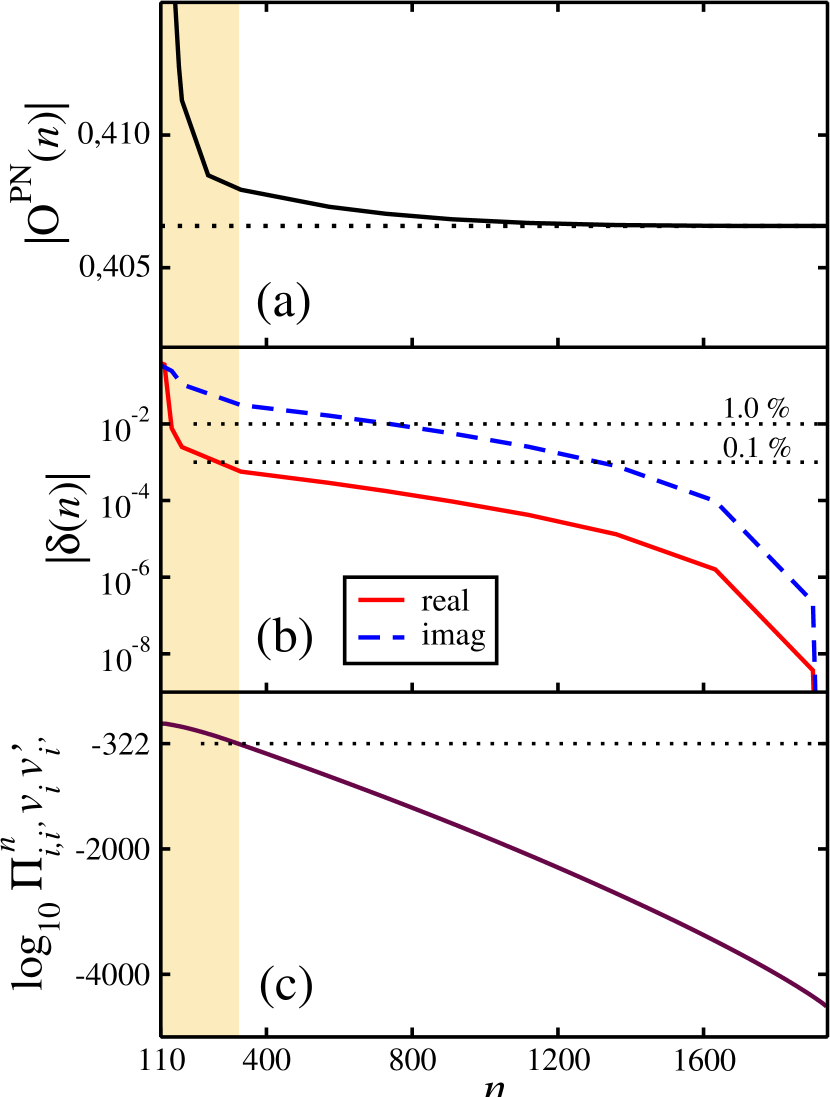
Figure 1: Matrix element ${\cal{O}}^{{\rm PN}}(n)$ as a function of the number of canonical basis states included in the computation $n$. Panel (a) shows the modulus of the matrix elements at $\phi=\pi/10$ as a function of $n$. The dotted-line corresponds to the value in the full model space when $n=N$. Panel (b) shows the absolute value of the relative error $\delta(n)$ for both the real part (full line) and imaginary part (dashed-line) of the matrix element (see text). The two horizontal dotted-lines indicate the error at 1% and 0.1%. Panel (c) shows the decimal logarithm of the denominator of the prefactor in Eq. (1). The horizontal dotted-line indicates the value $10^{-322}$, which corresponds approximately to the smallest number that can be represented using the double-precision data type. The shadded area represents the range of validity of using Eq. (1) to compute the overlap at the double-precision level.

Example. As a proof of principle, we now show results for the computation of a matrix element involved in the particle-number projection method for an even-$A$ nucleus. We denote this matrix element ${\cal O}^{{\rm PN}}$:

$${\cal{O}}^{{\rm PN}}\equiv\langle\Phi|e^{-i\hat{N}\phi}|\Phi\rangle=\langle\Phi|\Phi^{\prime}\rangle$$ (21)

where $e^{-i\hat{N}\phi}$ is the gauge rotational operator for the particle number projection, $\hat{N}$ the particle number operator and $\phi$ the gauge angle. We focus on projecting the number of neutrons and generate the occupation numbers with a HFB calculation of ¹⁹²Pb using a basis of 17 major oscillator shells, the SLY4 functional (Chabanat et al., 1998) and a separable Gaussian pairing interaction (Veselý et al., 2012). We rewrite ${\cal O}^{{\rm PN}}$ as the overlap between the vacuum $|\Phi\rangle$ and a rotated vacuum $|\Phi^{\prime}\rangle$ with the corresponding Bogoliubov-transformation matrices $U^{\prime}=Ue^{i\phi}$ and $V^{\prime}=Ve^{-i\phi}$. We set $\phi=\pi/10$ and for convenience, we randomly generate the unitary matrices $D$ and $C$. We calculate ${\cal{O}}^{{\rm PN}}$ with Eq. (11) for different values of the number $n$ of canonical basis states including in the computation (we label ${\cal{O}}^{{\rm PN}}(n)$ the values obtained when $n$ states are included). The exact value is obtained for $n=N=$1938 i.e. when all single particle states have been included. Results of the calculation are shown in Fig. (1). Panel (a) shows the modulus of the matrix elements as a function of $n$ and as one can see, the value of the matrix elements smoothly converges to the exact value as $n$ is increased. Panel (b) shows the modulus of the real and imaginary part of the relative error defined as $\delta(n)=({\cal{O}}^{{\rm PN}}(n)-{\cal{O}}^{{\rm PN}}(N))/|{\cal{O}^{{\rm PN}}}(N)|$. In order to have a relative error less than one percent around 800 states are needed. Panel (c) shows the decimal logarithm of $\prod_{i,i^{\prime}}^{n}v_{i}v^{\prime}_{i^{\prime}}$ i.e. the denominator of the prefactor of Eq. (1) as a function of $n$. The horizontal dashed-line and arrow indicate the value $10^{-322}$, below which the computation of the overlap with Eq. (1) is numerically unstable when computed with the double-precision data type. In such a case, the computation limit is reached at $n=323$ for which $v_{i}=0.097593$. Increasing the numerical precision would allow to extend the range of validity of using Eq. (1) to compute the overlap albeit at the price of a higher computational burden. Since in the general case the product $\prod_{i,i^{\prime}}^{n}v_{i}v^{\prime}_{i^{\prime}}$ may become arbitrary small, any calculation of Eq. (1) with increased precision will eventually fail.

With the new formula all states can be included without encountering any numerical instability. The ability to include all states is expected to be particularly important for the description of the radial tail of the wavefunction. A correct description of the wavefunction at large distances is in turn critical for many applications involving scattering and reaction processes (Johnson et al., 2020) such as alpha decay (Ward et al., 2013) or the computation of nucleon-nucleus optical potential (Rotureau et al., 2018; Rotureau, 2020; Idini et al., 2019).

Conclusion. In this Letter we have presented a new, exact and numerically stable formulation of overlap functions that appear in beyond mean-field theories such as the GCM method. We have illustrated the benefits offered by this formulation by computing a matrix element for the particle-number projection method. We want to emphasize that the derivations presented here are applicable to overlap functions in the context of both even and odd number parity.

The expression for the overlap can be combined with approaches to obtain the matrix elements of the Hamiltonian for example by expressing these matrix elements in a factorized form as sums of products of transition densities multiplied by overlap functions (Ring and Schuck, 1980; Hu et al., 2014). Such transition densities are efficiently calculated in the canonical basis where dimensions can be reduced by removing unoccupied states (Yao et al., 2009; Bonche et al., 1990; Heenen et al., 1993; Valor et al., 2000; Tagami and Shimizu, 2012). The expressions derived in this letter may also be extended to cover cases when the left and right vacua are expressed in different bases ( see e.g. (Avez and Bender, 2012; Robledo, 2011)).

The new formula offers substantial improvements over current methods since exact values can now be obtained even in large spaces without being limited by the ability of representing very small or large numbers. It adds no extra computational effort or complexity and may be truncated in a systematic way, which allows for a smooth convergence towards the exact value. Finally, the new formula opens the door towards precision calculations of nuclear reactions and nuclear structure where one takes advantage of the power of symmetry breaking.

We acknowledge beneficial discussions with Andrea Idini. The authors thank the Knut and Alice Wallenberg Foundation (KAW 2015.0021) and the Crawfoord foundation for financial support.

References

- Bertsch and Robledo (2012) G. F. Bertsch and L. M. Robledo, Phys. Rev. Lett. 108, 042505 (2012).
- Bender et al. (2003) M. Bender, P.-H. Heenen, and P.-G. Reinhard, Rev. Mod. Phys. 75, 121 (2003).
- Möller et al. (2006) P. Möller, R. Bengtsson, B. G. Carlsson, P. Olivius, and T. Ichikawa, Phys. Rev. Lett. 97, 162502 (2006).
- Frauendorf (2001) S. Frauendorf, Rev. Mod. Phys. 73, 463 (2001).
- Ring and Schuck (1980) P. Ring and P. Schuck, The nuclear many-body problem (Springer-Verlag, New York, 1980).
- Bender and Heenen (2008a) M. Bender and P.-H. Heenen, Phys. Rev. C 78, 024309 (2008a).
- Yao et al. (2020) J. M. Yao, B. Bally, J. Engel, R. Wirth, T. R. Rodríguez, and H. Hergert, Phys. Rev. Lett. 124, 232501 (2020).
- Malli and Ishikawa (1998) G. L. Malli and Y. Ishikawa, The Journal of Chemical Physics 109, 8759 (1998).
- Trsic et al. (2004) M. Trsic, W. F. Angelotti, and F. A. Molfetta, in A Tribute Volume in Honor of Professor Osvaldo Goscinski, Advances in Quantum Chemistry, Vol. 47 (Academic Press, 2004) pp. 315–329.
- Orestes et al. (2007) E. Orestes, K. Capelle, A. B. F. da Silva, and C. A. Ullrich, The Journal of Chemical Physics 127, 124101 (2007).
- Såmark-Roth et al. (2021) A. Såmark-Roth, D. M. Cox, D. Rudolph, L. G. Sarmiento, B. G. Carlsson, J. L. Egido, P. Golubev, J. Heery, A. Yakushev, S. Åberg, H. M. Albers, M. Albertsson, M. Block, H. Brand, T. Calverley, R. Cantemir, R. M. Clark, C. E. Düllmann, J. Eberth, C. Fahlander, U. Forsberg, J. M. Gates, F. Giacoppo, M. Götz, S. Götz, R.-D. Herzberg, Y. Hrabar, E. Jäger, D. Judson, J. Khuyagbaatar, B. Kindler, I. Kojouharov, J. V. Kratz, J. Krier, N. Kurz, L. Lens, J. Ljungberg, B. Lommel, J. Louko, C.-C. Meyer, A. Mistry, C. Mokry, P. Papadakis, E. Parr, J. L. Pore, I. Ragnarsson, J. Runke, M. Schädel, H. Schaffner, B. Schausten, D. A. Shaughnessy, P. Thörle-Pospiech, N. Trautmann, and J. Uusitalo, Phys. Rev. Lett. 126, 032503 (2021).
- Onishi and Yoshida (1966) N. Onishi and S. Yoshida, Nuclear Physics 80, 367 (1966).
- Neergård and Wüst (1983) K. Neergård and E. Wüst, Nuclear Physics A 402, 311 (1983).
- Haider and Gogny (1992) Q. Haider and D. Gogny, Journal of Physics G: Nuclear and Particle Physics 18, 993 (1992).
- Dönau (1998) F. Dönau, Physical Review C - Nuclear Physics 58, 872 (1998).
- Bender and Heenen (2008b) M. Bender and P.-H. Heenen, Phys. Rev. C 78, 024309 (2008b).
- Hara et al. (1982) K. Hara, A. Hayashi, and P. Ring, Nuclear Physics A 385, 14 (1982).
- Oi and Tajima (2005) M. Oi and N. Tajima, Physics Letters B 606, 43 (2005).
- Rodríguez and Egido (2010) T. R. Rodríguez and J. L. Egido, Phys. Rev. C 81, 064323 (2010).
- Bally and Duguet (2018) B. Bally and T. Duguet, Phys. Rev. C 97, 024304 (2018).
- Mizusaki et al. (2018) T. Mizusaki, M. Oi, and N. Shimizu, Physics Letters B 779, 237 (2018).
- Avez and Bender (2012) B. Avez and M. Bender, Phys. Rev. C 85, 034325 (2012).
- Schmid (2004) K. Schmid, Progress in Particle and Nuclear Physics 52, 565 (2004).
- Robledo (2009) L. M. Robledo, Phys. Rev. C 79, 021302(R) (2009).
- Bloch and Messiah (1962) C. Bloch and A. Messiah, Nuclear Physics A 39, 95 (1962).
- Gao et al. (2014) Z.-C. Gao, Q.-L. Hu, and Y. Chen, Physics Letters B 732, 360 (2014).
- Robledo (2011) L. M. Robledo, Phys. Rev. C 84, 014307 (2011).
- (28) See Supplementary material for details, which includes Refs Lieb (1968); Caianiello (1973) .
- Note (1) The matrix being skew symmetric, we do not write its lower triangle part.
- Chabanat et al. (1998) E. Chabanat, P. Bonche, P. Haensel, J. Meyer, and R. Schaeffer, Nuclear Physics A 635, 231 (1998).
- Veselý et al. (2012) P. Veselý, J. Toivanen, B. G. Carlsson, J. Dobaczewski, N. Michel, and A. Pastore, Phys. Rev. C 86, 024303 (2012).
- Johnson et al. (2020) C. W. Johnson, K. D. Launey, N. Auerbach, S. Bacca, B. R. Barrett, C. Brune, M. A. Caprio, P. Descouvemont, W. H. Dickhoff, C. Elster, P. J. Fasano, K. Fossez, H. Hergert, M. Hjorth-Jensen, L. Hlophe, B. Hu, R. M. I. Betan, A. Idini, S. Koenig, K. Kravvaris, D. Lee, J. Lei, A. Mercenne, R. N. Perez, W. Nazarewicz, F. Nunes, M. Ploszajczak, J. Rotureau, G. Rupak, A. M. Shirokov, I. J. Thompson, J. P. Vary, A. Volya, F. Xu, R. G. T. Zegers, V. Zelevinsky, and X. Zhang, Journal of Physics G: Nuclear and Particle Physics (2020).
- Ward et al. (2013) D. E. Ward, B. G. Carlsson, and S. Åberg, Phys. Rev. C 88, 064316 (2013).
- Rotureau et al. (2018) J. Rotureau, P. Danielewicz, G. Hagen, G. R. Jansen, and F. M. Nunes, Phys. Rev. C 98, 044625 (2018).
- Rotureau (2020) J. Rotureau, Frontiers in Physics 8, 285 (2020).
- Idini et al. (2019) A. Idini, C. Barbieri, and P. Navrátil, Phys. Rev. Lett. 123, 092501 (2019).
- Hu et al. (2014) Q.-L. Hu, Z.-C. Gao, and Y. Chen, Physics Letters B 734, 162 (2014).
- Yao et al. (2009) J. M. Yao, J. Meng, P. Ring, and D. P. Arteaga, Phys. Rev. C 79, 044312 (2009).
- Bonche et al. (1990) P. Bonche, J. Dobaczewski, H. Flocard, P.-H. Heenen, and J. Meyer, Nuclear Physics A 510, 466 (1990).
- Heenen et al. (1993) P.-H. Heenen, P. Bonche, J. Dobaczewski, and H. Flocard, Nuclear Physics A 561, 367 (1993).
- Valor et al. (2000) A. Valor, P.-H. Heenen, and P. Bonche, Nuclear Physics A 671, 145 (2000).
- Tagami and Shimizu (2012) S. Tagami and Y. R. Shimizu, Progress of Theoretical Physics 127, 79 (2012), https://academic.oup.com/ptp/article-pdf/127/1/79/19572858/127-1-79.pdf .
- Lieb (1968) E. H. Lieb, Journal of Combinatorial Theory 5, 313 (1968).
- Caianiello (1973) E. R. Caianiello, Combinatorics and renormalization in quantum field theory (W. A. Benjamin Reading, Mass, 1973).