Device-independent quantification of measurement incompatibility

Abstract

Incompatible measurements, i.e., measurements that cannot be simultaneously performed, are necessary to observe nonlocal correlations. It is natural to ask, e.g., how incompatible the measurements have to be to achieve a certain violation of a Bell inequality. In this work, we provide the direct link between Bell nonlocality and the quantification of measurement incompatibility. This includes quantifiers for both incompatible and genuine-multipartite incompatible measurements. Our method straightforwardly generalizes to include constraints on the system’s dimension (semi-device-independent approach) and on projective measurements, providing improved bounds on incompatibility quantifiers, and to include the prepare-and-measure scenario.

I Introduction

One of the most intriguing phenomena in quantum theory is that there exist physical quantities whose values cannot be simultaneously obtained. The most celebrated example is arguably the position and momentum of a particle, initially formulated in terms of the uncertainty relation Heisenberg (1927); Robertson (1929); Busch et al. (2014). Such a phenomenon, called measurement incompatibility (or simply incompatibility), enables one to demonstrate several remarkable quantum features such as quantum nonlocality Bell (1964); Brunner et al. (2014), quantum steering Schrödinger (1935); Cavalcanti and Skrzypczyk (2017); Uola et al. (2020), quantum contextuality Kochen and Specker (1967); Klyachko et al. (2008); Cabello (2008); Liang et al. (2011a); Budroni et al. (2021) (see, respectively, Wolf et al. (2009), Quintino et al. (2014); Uola et al. (2014), and Xu and Cabello (2019); Tavakoli and Uola (2020)), and provides a resource to many quantum information protocols (see, e.g., Carmeli et al. (2019); Skrzypczyk et al. (2019); Uola et al. (2019); Takagi et al. (2019); Takagi and Regula (2019); Oszmaniec and Biswas (2019); Mori (2020); Buscemi et al. (2020)). In a more modern language, incompatibility has been formulated as the non-existence of a joint measurement Lahti (2003).

Nonlocality plays a central role in quantum information (QI), more precisely, in the definition of device-independent (DI) QI Acín et al. (2007); Scarani (2012); Brunner et al. (2014): without any characterization of the measurement devices (e.g., measurement operators, states, system dimension) all information is encoded in $P(a,b|x,y)$, the probability of the outputs $a,b$ given the measurement settings $x,y$. Provided that $P(a,b|x,y)$ is nonlocal, a surprisingly high variety of statements and QI protocols can be based on such correlations: from quantum key distribution Acín et al. (2007), to entanglement detection Moroder et al. (2013), randomness certification Pironio et al. (2010a), verification of steerability Wiseman et al. (2007); Cavalcanti and Skrzypczyk (2016); Chen et al. (2016, 2018), witnessing dimension of quantum systems Gallego et al. (2010), and so on.

In this sense, a violation of a Bell inequality is also a DI witness of incompatibility, as incompatible measurements are necessary to observe it Wolf et al. (2009); Hirsch et al. (2018); Bene and Vértesi (2018). In this work, we address the quantitative question: How incompatible the underlying measurements have to be in order to observe a certain quantum violation of a Bell inequality? A central tool in our investigation is the notion of moment matrix, that has wide applications in the characterization of quantum correlations and DI approaches  Doherty et al. (2008); Navascués et al. (2007); Pironio et al. (2010b); Moroder et al. (2013). Here, we introduce the measurement moment matrix (MMM) that allows us to quantify several quantities that are formulated via semidefinite programming (SDP) Boyd and Vandenberghe (2004) in terms of measurement effects, such as incompatibility robustness Haapasalo (2015); Uola et al. (2015); Heinosaari et al. (2016), genuine-multipartite incompatibility Quintino et al. (2019), and similar quantities Pusey (2015); Heinosaari et al. (2015); Cavalcanti and Skrzypczyk (2016).

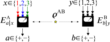
Figure 1: Schematic representation of device-independent quantification of measurement incompatibility. By performing measurements on two distant particles and observing the correlations $P(a,b|x,y)$, we are able to estimate several measures of incompatiblity among pairs, $({\color[rgb]{1,0,0}1},{\color[rgb]{0.2,0.2,0.8}2})$, $({\color[rgb]{1,0,0}1},{\color[rgb]{0.2,0.6,0.2}3})$, $(\color[rgb]{0.2,0.2,0.8}{2},{\color[rgb]{0.2,0.6,0.2}3})$, or triples, $({\color[rgb]{1,0,0}1},{\color[rgb]{0.2,0.2,0.8}2},{\color[rgb]{0.2,0.6,0.2}3})$, or genuine triplewise incompatibility among $({\color[rgb]{1,0,0}1},{\color[rgb]{0.2,0.2,0.8}2},{\color[rgb]{0.2,0.6,0.2}3})$.

Our results allows for investigations beyond the DI scenario. In fact, due to its generality the idea of MMMs can be straightforwardly extended to the semi-DI approach, i.e., where the dimension of quantum system is assumed to be known Pawłowski and Brunner (2011); Liang et al. (2011b), to investigate the role of dimension constraints or even non-projectivness in measurement incompatibility, and it can be extended even to the prepare-and-measure scenario.

II Incompatible measurements

Let us start by briefly reviewing the concept of measurement incompatibility. Consider a quantum measurement described by a positive-operator-valued measure (POVM) $\{{E^{\text{A}}_{a|x}}\}_{a}$ for a given $x$, where the indices $x\in\mathcal{X}$ and $a\in\mathcal{A}$, label the measurement settings and outcomes of the measurement, respectively. The operators ${E^{\text{A}}_{a|x}}$, called effect operators are positive semidefinite, i.e., ${E^{\text{A}}_{a|x}}\succeq 0~{}\forall a,x$, and satisfy the normalization condition, $\sum_{a}{E^{\text{A}}_{a|x}}=\openone~{}\forall x$. A collection of POVMs $\{{E^{\text{A}}_{a|x}}\}_{a,x}$ is called a measurement assemblage Piani and Watrous (2015). A measurement assemblage is said to be compatible or jointly measurable if it can be written as Busch et al. (1996); Ali et al. (2009)

$${E^{\text{A}}_{a|x}}=\sum_{\lambda}P(a|x,\lambda)G_{\lambda}\quad\forall a,x,$$ (1)

where $\{G_{\lambda}\}_{\lambda}$ is a valid POVM and $P(a|x,\lambda)$ are non-negative numbers such that $\sum_{a}P(a|x,\lambda)=1$ for all $x,\lambda$. Physically, joint measurability means that the statistic of each POVM in the assemblage can be obtained by classically post-processing the statistic of a parent POVM $\{G_{\lambda}\}_{\lambda}$, irrespective of the state.

Several incompatibility measures have been proposed in the literature (see Ref. Designolle et al. (2019) for an overview). Here, we choose the incompatibility robustness Haapasalo (2015); Uola et al. (2015); Heinosaari et al. (2016) defined as

$$\begin{split}\mathcal{IR}(\{{E^{\text{A}}_{a|x}}\}):=\min\Big{\{}t\ \Big{|}\ \{({E^{\text{A}}_{a|x}}+t\cdot N_{a|x})/(1+t)\}_{a,x}\\ \text{ is jointly measurable }\Big{\}},\end{split}$$ (2)

where the minimum is take w.r.t. any arbitrary assemblage $\{N_{a|x}\}_{a,x}$. Here, $\mathcal{IR}$ is related to the minimum noise necessary for $\{{E^{\text{A}}_{a|x}}\}_{a,x}$ to become jointly measurable. From a quantum information perspective, $\mathcal{IR}$ quantifies the advantage that $\{{E^{\text{A}}_{a|x}}\}_{a,x}$ provides w.r.t. jointly measurable assemblages for a certain state-discrimination task Carmeli et al. (2019); Skrzypczyk et al. (2019); Uola et al. (2019); Takagi et al. (2019); Takagi and Regula (2019); Oszmaniec and Biswas (2019); Mori (2020). Moreover, it can be efficiently computed via SDP Uola et al. (2015); Boyd and Vandenberghe (2004):

$$\mathcal{IR}=\min_{\{G_{\lambda}\}} \frac{1}{d}\sum_{\lambda}\operatorname{tr}[G_{\lambda}]-1$$ (3)

$${\rm s.t.} G_{\lambda}\succeq 0\ \forall\lambda,\ \sum_{\lambda}\delta_{a,\lambda_{x}}G_{\lambda}\succeq{E^{\text{A}}_{a|x}}\ \forall a,x,\$$

$$\sum_{\lambda}G_{\lambda}=\frac{1}{d}\left(\sum_{\lambda}\operatorname{tr}[G_{\lambda}]\right)\cdot\openone,$$

where $\lambda:=(\lambda_{1},\lambda_{2},...,\lambda_{|\mathcal{X}|})$, $\lambda_{i}\in\mathcal{A}$, encodes the deterministic strategies.

III The measurement moment matrices

As first noted by Moroder et. al. Moroder et al. (2013), moment matrices can be interpreted as the application of a completely positive map to a (set of) positive operator(s), such as a quantum state Doherty et al. (2008); Navascués et al. (2007, 2008); Moroder et al. (2013) or steering state ensembles Chen et al. (2016, 2018). Here, we define the measurement moment matrices (MMMs) by applying a completely positive map on POVMs

$$\chi[{E^{\text{A}}_{a|x}}]:=\sum_{n}K_{n}({E^{\text{A}}_{a|x}}\otimes\openone^{\rm B})K_{n}^{\dagger}\quad\forall a,x,$$ (4)

where the map is obtained by first embedding the system ${\rm A}$ in the tensor product with a second identical system ${\rm B}$, i.e., ${E^{\text{A}}_{a|x}}\mapsto{E^{\text{A}}_{a|x}}\otimes\openone^{\rm B}$, which is a completely positive map, and then applying the Kraus operators $K_{n}:{\rm AB}\rightarrow\overline{\rm AB}$ defined as ${K_{n}:=\sum_{i}|i\rangle_{\overline{\rm AB}{\rm AB}}\langle n|({\varrho^{\text{AB}}})^{\frac{1}{2}}S_{i}}$, with $\{|i\rangle\}_{i}$ and $\{|n\rangle\}_{n}$ the orthonormal bases for the output space $\overline{\rm AB}$ and the input space ${\rm AB}$, respectively, and $\{S_{i}\}$ is a sequence of operators to be specified later. In this way, one obtains a moment matrix

$$\chi_{{\varrho^{\text{AB}}},\{S_{i}\}}[{E^{\text{A}}_{a|x}}]=\sum_{ij}|i\rangle\langle j|\operatorname{tr}\left[S_{i}({E^{\text{A}}_{a|x}}\otimes\openone^{\rm B})S_{j}^{\dagger}{\varrho^{\text{AB}}}\right]$$ (5)

for each $a,x$. In what follows, we simply use the symbol $\chi[{E^{\text{A}}_{a|x}}]$, or even $\chi$, when there is no risk of confusion. The MMM $\chi$ is a type of localizing matrix, proposed in the context of noncommutative polynomial optimization Pironio et al. (2010b), but here we define them from the perspective of measurement effects. In particular, their formulation is independent of the standard Navascués-Pironio-Acín (NPA) moment matrix Navascués et al. (2007, 2008).

We choose the operators $\{S_{i}\}$ as products of POVM elements, e.g., $\{S_{i}\}=\{{E^{\text{A}}_{a|x}}\otimes\openone^{\rm B},\openone^{\rm A}\otimes{E^{\text{B}}_{b|y}},{E^{\text{A}}_{a|x}}\otimes{E^{\text{B}}_{b|y}},{E^{\text{A}}_{a|x}}\otimes({E^{\text{B}}_{b|y}}E_{b^{\prime}|y^{\prime}}^{\text{B}}),{\rm etc.}\}$, and following the convention of Ref. Moroder et al. (2013): a level $\ell$ is denoted by $\{S_{i}^{(\ell)}\}:=\openone\cup\mathcal{O}^{(1)}\cup\mathcal{O}^{(2)}\cup,...,\cup\mathcal{O}^{(\ell)}$, where $\mathcal{O}^{(\ell)}:=\{E_{a_{1}|x_{1}}^{\text{A}}E_{a_{2}|x_{2}}^{\text{A}}...E_{a_{\ell-k}|x_{\ell-k}}^{\text{A}}\otimes E_{b_{\ell-k+1}|y_{\ell-k+1}}^{\text{B}}...E_{b_{\ell}|y_{\ell}}^{\text{B}}\}$ is composed of all $\ell$-order products of ${E^{\text{A}}_{a|x}}$’s and ${E^{\text{B}}_{b|y}}$’s. Even though the operators ${\varrho^{\text{AB}}},\{{E^{\text{A}}_{a|x}}\}_{a,x}$ and $\{{E^{\text{B}}_{b|y}}\}_{b,y}$ are uncharacterized, one is still able to obtain specific entries in $\chi$, such as those corresponding to accessible statistics in a DI setting, i.e., $P(a,b|x,y)=\operatorname{tr}({E^{\text{A}}_{a|x}}\otimes{E^{\text{B}}_{b|y}}{\varrho^{\text{AB}}})$. Moreover, by the Neumark dilation Peres (1990), any POVM can be realized by a projective measurement in a higher dimensional space, implying conditions such as $0=\operatorname{tr}({E^{\text{A}}_{a|x}}E_{a^{\prime}|x}^{\text{A}}\otimes{E^{\text{B}}_{b|y}})$, for $a^{\prime}\neq a$, or $0=\operatorname{tr}({E^{\text{A}}_{a|x}}\otimes{E^{\text{B}}_{b|y}}E_{b^{\prime}|y}^{\rm B})$, for $b^{\prime}\neq b$. Moreover, since the MMMs are obtained by applying a completely positive map on valid POVMs (see Eq. (4)), each $\chi$ is positive semidefinite by construction. It is convenient to decompose $\chi$ into the characterized parts and unknown parts Moroder et al. (2013):

$$\chi =\chi^{\rm fixed}(P)+\chi^{\rm open}(u)$$ (6)

$$=\sum_{a,b,x,y}P(a,b|x,y)F_{a,b,x,y}+\sum_{v}u_{v}F_{v},$$

where all of $F_{a,b,x,y}$ and $F_{v}$ are symmetric matrices. The complex numbers $u_{v}$ represent all the uncharacterized variables.

IV Device-independent quantification of measurement incompatibility

Via the MMM, we are able to define, for any SDP involving effect operators, its DI relaxation, i.e., another version of the problem involving only DI assumptions. As an example, we will show below how to define the incompatibility robustness. Several other examples, such as incompatibility jointly measurable robustness, incompatibility probabilistic robustness, incompatibility random robustness, and the incompatibility weight, are described in App. A. The problem in Eq. (3) is mapped to

$$\min_{\{\chi[G_{\lambda}],\chi[E_{a|x}]\}_{\lambda,a,x}} \sum_{\lambda}\chi[G_{\lambda}]_{\openone}-1$$ (7)

$${\rm s.t.} \sum_{\lambda}\delta_{a,\lambda_{x}}\chi[G_{\lambda}]\ \succeq\chi[{E^{\text{A}}_{a|x}}]\quad\forall a,x,$$

$$\chi[G_{\lambda}]\succeq 0\quad\forall\lambda,$$

$$\sum_{\lambda}\chi[G_{\lambda}]=\sum_{\lambda}\chi[G_{\lambda}]_{\openone}\cdot\chi[\openone],$$

$$\sum_{a}\chi[{E^{\text{A}}_{a|x}}]=\chi[\openone]\quad\forall x,$$

$$\chi[{E^{\text{A}}_{a|x}}]\succeq 0\quad\forall a,x,$$

$$P(a,b|x,y)=P_{\rm obs}(a,b|x,y)\quad\forall a,b,x,y,$$

where $\chi[G_{\lambda}]_{\openone}:=\operatorname{tr}(G_{\lambda}\otimes\openone^{\rm B}{\varrho^{\text{AB}}})$. The objective function is the same as that of Eq. (3) due to the fact that ${\operatorname{tr}(\sum_{\lambda}G_{\lambda}\otimes\openone^{\rm B}{\varrho^{\text{AB}}})=\operatorname{tr}[\big{(}\sum_{\lambda}\operatorname{tr}(G_{\lambda})\big{)}\openone^{\rm A}\otimes\openone^{\rm B}{\varrho^{\text{AB}}}]/d}=(1/d)\sum_{\lambda}\operatorname{tr}(G_{\lambda})$. The first three constrains are directly obtained from the three constraints in Eq. (3). The rest are associated with, respectively, normalization of POVMs, positivity of POVMs, and the observed nonlocal correlation. The above problem is not an SDP yet, since the third constraint in Eq. (7) is quadratic. To tackle this problem, we relax the third constraint by keeping only the characterized terms in $\chi[\openone]$. Namely, the relaxed constraint becomes: $\sum_{\lambda}\chi[G_{\lambda}]^{\rm fixed}=\sum_{\lambda}\chi[G_{\lambda}]_{\openone}\cdot\chi[\openone]^{\rm fixed}$, where, with some abuse of notation (since no elements in $\chi[G_{\lambda}]$ are actually fixed), we mean to retain only the constraints associated with entries in $\chi[\openone]^{\rm fixed}$ as in Eq. (6), i.e., with the observed probabilities $P_{\rm obs}(a,b|x,y)$.

Given $$P_{\rm obs}(a,b|x,y)$$ (8)

$$\min_{\chi[\openone],\{\chi[G_{\lambda}],\chi[E_{a|x}]\}_{\lambda,a,x}} \sum_{\lambda}\chi[G_{\lambda}]_{\openone}-1$$

$${\rm s.t.} \sum_{\lambda}\delta_{a,\lambda_{x}}\chi[G_{\lambda}]\ \succeq\chi[{E^{\text{A}}_{a|x}}]\quad\forall a,x,$$

$$\chi[G_{\lambda}]\succeq 0\quad\forall\lambda,$$

$$\sum_{\lambda}\chi[G_{\lambda}]^{\rm fixed}=\sum_{\lambda}\chi[G_{\lambda}]_{\openone}\cdot\chi[\openone]^{\rm fixed},$$

$$\sum_{a}\chi[{E^{\text{A}}_{a|x}}]=\chi[\openone]\quad\forall x,$$

$$\chi[{E^{\text{A}}_{a|x}}]\succeq 0\quad\forall a,x,$$

$$P(a,b|x,y)=P_{\rm obs}(a,b|x,y),$$

$$\forall a,b,x,y,$$

The solution obtained above, denoted by $\mathcal{IR_{\rm DI}}$, is a lower bound on $\mathcal{IR}$ of the underlying measurement assemblage. In other words, it tells us the minimum degree of measurement incompatibility present when observing a certain nonlocal correlation.

An analogous SDP can be used for bounding from below the measurements incompatibility necessary for a given violation of Bell inequality. In this case, only the Bell value, i.e., $I(P)$, is given and not $P_{\rm obs}(a,b|x,y)$. As a consequence one simply removes entirely the third constraint in Eq. (7), as $\chi[\openone]^{\rm fixed}$ is not characterized. Alternatively, by changing the objective function one may ask what is the maximal violation of a Bell inequality for a given value $\mathcal{IR}_{0}$ of the robustness. It can be easily shown that for each pair $(I(P),\mathcal{IR}_{0})$ a feasible solution of one SDP is also a feasible solution of the other, hence, they characterize the same set. See App. B for more details.

The formulation with the fixed $\mathcal{IR}_{0}$, however, turns out to more more convenient, as it removes the nonlinearity in the previous SDP. In fact, the substitution $\sum_{\lambda}\chi[G_{\lambda}]_{\openone}-1=\mathcal{IR}_{0}$, allows us to write the third constraint of Eq. (7) as $\sum_{\lambda}\chi[G_{\lambda}]=(\mathcal{IR}_{0}+1)\chi[\openone]$. We then have

Given $$\mathcal{IR}_{0}$$ (9)

$$\max_{\chi[\openone],\{\chi[G_{\lambda}],\chi[E_{a|x}]\}_{\lambda,a,x}} I(P)$$

$${\rm s.t.} \sum_{\lambda}\delta_{a,\lambda_{x}}\chi[G_{\lambda}]\ \succeq\chi[{E^{\text{A}}_{a|x}}]\quad\forall a,x,$$

$$\chi[G_{\lambda}]\succeq 0\quad\forall\lambda,$$

$$\sum_{\lambda}\chi[G_{\lambda}]=(\mathcal{IR}_{0}+1)\chi[\openone],$$

$$\sum_{a}\chi[{E^{\text{A}}_{a|x}}]=\chi[\openone]\quad\forall x,$$

$$\chi[{E^{\text{A}}_{a|x}}]\succeq 0\quad\forall a,x,$$

$$\sum_{\lambda}\chi[G_{\lambda}]_{\openone}=\mathcal{IR}_{0}+1,$$

We apply this method to the tilted-CHSH inequality Acín et al. (2012), see the next section for a detailed explanation and Fig. 2 for a summary of the results. What we want to highlight now, is that for the simple case analyzed in Fig. 2, the SDP in Eq. (7) already provides an exact solution, despite the relaxation of the nonlinear constraint. In contrast, for the case of genuine multipartite incompatibility robustness, discussed in Sec. VI below, we see that different bounds arise when the same constraint is taken into account or not, see also Apps. C and D.

V Quantification of incompatibility robustness

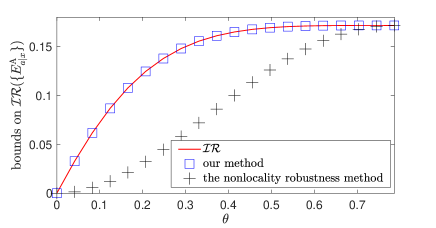
Figure 2: DI $\mathcal{IR}$ bounds with the MMM method and the nonlocal robustness (NLR). Red curve: $\mathcal{IR}$ of Bob’s optimal measurements for the tilted-CHSH inequality. Blue squares: DI lower bound from the MMM method ($2$nd level of the hierarchy). Black crosses: lower bound from NLR.

As a first application of our method, we consider the simplest Bell scenario, i.e., the Clauser-Horne-Shimony-Holt (CHSH) scenario. More precisely, we consider the tilted-CHSH Acín et al. (2012) (see also Yang and Navascués (2013); Bamps and Pironio (2015)) inequality, parametrized by $\alpha$, namely, $I_{\rm CHSH}^{\rm tilted}:=\alpha\langle A_{1}\rangle+\langle A_{1}B_{1}\rangle+\langle A_{1}B_{2}\rangle+\langle A_{2}B_{1}\rangle-\langle A_{2}B_{2}\rangle\stackrel{{\scriptstyle\mathcal{L}}}{{\leq}}2+\alpha$, with $\langle A_{x}\rangle:=P_{\rm A}(a=1|x)-P_{\rm A}(a=-1|x)$ and $\langle A_{x}B_{y}\rangle:=P(a=b|x,y)-P(a\neq b|x,y)$ being the correlators. The maximal quantum violation, $\sqrt{8+2\alpha^{2}}$, is achieved with two fixed Pauli measurement on Alice’s side, i.e., $\hat{X}$ and $\hat{Z}$, and tilted measurements for Bob, i.e., $\cos\mu\hat{Z}+\sin\mu\hat{X},\cos\mu\hat{Z}-\sin\mu\hat{X}$ on the partially entangled state $|\psi_{\theta}\rangle=\cos\theta|00\rangle+\sin\theta|11\rangle$, with $\mu=\arctan(\sin 2\theta)$ and $\theta=(1/2)\arctan(\sqrt{(4-\alpha^{2})/2\alpha^{2}})$.

For each value of $\alpha$ one can obtain the optimal state and the optimal pair of measurements (unique up to local isometries) providing the maximal quantum violation. The value of Bob’s robustness for a given $\theta$ coincides with its DI bound computed via the MMM assuming the corresponding distribution $P(a,b|x,y)$ (see Fig. 2). In the same figure, we also plot the DI bound of $\mathcal{IR}$ obtained via the nonlocality robustness (NLR) Cavalcanti and Skrzypczyk (2016) method. The NLR method, as well as another method proposed for the DI lower bound of incompatibility, i.e., the assemblage moment matrix (AMM) Chen et al. (2016, 2018) method, are based on the connection between steering and incompatibility Uola et al. (2014, 2015); Quintino et al. (2014). In contrast, the MMM relies on the construction of a moment matrix directly from the measurement operators. In App. E, we show that the AMM can be identified with a special case of a MMM. Hence, it can never provide a better bound for incompatibility. In addition, we explicitly show via the $I_{3322}$ inequality Collins and Gisin (2004), that the MMM provides strictly better bounds.

VI Quantification of genuine multipartite incompatibility robustness

Here, we show how the MMM can be used to quantify the genuine multipartite incompatibility robustness (GMIR) recently introduced by Quintino et al. Quintino et al. (2019). An example is provided in Fig. 3 for different Bell inequalities. All the results presented, use the maximization of the Bell violation for a given robustness, see Eq. (VI) below. As we discuss in App. C, the results obtained with this method are provable better than those obtained minimizing the robustness for a given Bell violation. Finally, in addition to being able to quantify the GMIR, our method can also improve the thresholds for its detection. We compare ours with those computed in Ref. Quintino et al. (2019).

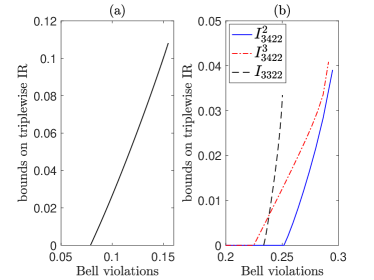
Figure 3: MMMs can also be used to compute lower bounds on genuine triplewise $\mathcal{IR}$ in a DI setting. (a) DI lower bounds on genuine triplewise $\mathcal{IR}$ in the elegant Bell scenario. (b)The black-dashed, red-dash-dotted, and blue-solid curves represent, respectively, DI lower bounds on genuine triplewise $\mathcal{IR}$ in the $I_{3322}$, $I_{3422}^{3}$, and $I_{3422}^{2}$ scenarios. The SDP carrying out the computation can be found in Eq. (VI).

A measurement assemblage of three measurements $\{\{E_{a|x}\}_{a}\}_{x=1,2,3}$ is said to be genuinely triplewise incompatible Quintino et al. (2019) if it is impossible to write it as a convex mixture of three measurement assemblages, each containing a different pair of compatible measurements Quintino et al. (2019). More concretely, if there exists three assemblages $\{\{J_{a|x}^{st}\}_{a}\}_{x=1,2,3}$ for $(s,t)=(1,2),(1,3),(2,3)$ such that $\{J_{a|s}^{st}\}_{a}$ and $\{J_{a|t}^{st}\}_{a}$ are jointly measurable for any pair $s,t$ and each $E_{a|x}$ can be written as

$$E_{a|x}=p_{12}J^{12}_{a|x}+p_{23}J^{23}_{a|x}+p_{13}J^{13}_{a|x}$$ (10)

for some probabilities $p_{12}$, $p_{23}$, and $p_{13}$ that respect $p_{12}+p_{23}+p_{13}=1$, we will say that $\{\{E_{a|x}\}_{a}\}_{x=1,2,3}$ are not genuine triplewise incompatible.

This condition can be written in a SDP form (see Ref. Quintino et al. (2019) and App. C for a brief self-contained summary), which leads to a SDP formulation of the robustness as

Given $$\{E_{a|x}\}_{a,x},$$

and variables $$\{G^{12}_{\lambda},G^{13}_{\lambda},G^{23}_{\lambda}\}_{\lambda},\{J_{a|3}^{12},J_{a|2}^{13},J_{a|1}^{23}\}_{a},$$

$$\min\ \frac{1}{d}\sum_{\lambda}\operatorname{tr}[G^{12}_{\lambda}+G^{13}_{\lambda}+G^{23}_{\lambda}]-1$$ (11)

s.t. $$G^{st}_{\lambda}\succeq 0\ \forall\lambda,\ \sum_{\lambda}G^{st}_{\lambda}=\frac{\openone}{d}\sum_{\lambda}\operatorname{tr}[G^{st}_{\lambda}]$$

$$\text{ for }(s,t)=(1,2),(1,3),(2,3);$$

$$J^{st}_{a|x}\succeq 0,\ \forall a,\ \sum_{a}J^{st}_{a|x}=\sum_{\lambda}G^{st}_{\lambda}\text{ and }$$

$$\sum_{\lambda}\delta_{a,\lambda_{x}}(G^{sx}_{\lambda}+G^{tx}_{\lambda})+J^{st}_{a|x}\succeq E_{a|x},$$

$$\text{ for }(s,t,x)=(1,2,3),(1,3,2),(2,3,1);$$

Applying the same argument as the one for the standard incompatibility robustness above SDP can have a DI relaxation via moment matrices

Given $$P_{\rm obs}(a,b|x,y),\text{ and }$$

variables $$\{\chi[E_{a|x}]\}_{a,x},\text{ and }\{\chi[G^{st}_{\lambda}]\}_{\lambda},\{\chi[J^{st}_{a|x}]\}_{a},$$

$$\text{ for }(s,t,x)=(1,2,3),(1,3,2),(2,3,1);$$

$$\min\ \sum_{\lambda}\chi[G^{12}_{\lambda}]_{\openone}+\chi[G^{13}_{\lambda}]_{\openone}+\chi[G^{23}_{\lambda}]_{\openone}-1$$

s.t. $$\chi[G^{st}_{\lambda}]\succeq 0\ \forall\lambda,(s,t)=(1,2),(1,3),(2,3);$$

$$\sum_{\lambda}\chi[G^{st}_{\lambda}]^{\rm fixed}=\chi[\openone]^{\rm fixed}\sum_{\lambda}\chi[G^{st}_{\lambda}]_{\openone}\$$

$$\text{ for }(s,t)=(1,2),(1,3),(2,3);$$

$$\chi[J^{st}_{a|x}]\succeq 0,\ \forall a,\ \sum_{a}\chi[J^{st}_{a|x}]=\sum_{\lambda}\chi[G^{st}_{\lambda}]\text{ and }$$

$$\sum_{\lambda}\delta_{a,\lambda_{x}}(\chi[G^{sx}_{\lambda}]+\chi[G^{tx}_{\lambda}])+\chi[J^{st}_{a|x}]\succeq\chi[E_{a|x}],$$

$$\text{ for }(s,t,x)=(1,2,3),(1,3,2),(2,3,1);$$

$$\chi[E_{a|x}]\succeq 0,\text{ for all }a,x,$$

$$\sum_{a}\chi[E_{a|x}]=\chi[\openone],\text{ for all }x,$$

$$P(a,b|x,y)=P_{\rm obs}(a,b|x,y).$$ (12)

Again, one can compute the maximum of a Bell inequality $I(P)$ for a given robustness $\mathcal{IR}_{0}$ as

Given $$\ \mathcal{IR}_{0},\text{ and }$$

variables $$\{\chi[E_{a|x}]\}_{a,x},\{\chi[G^{st}_{\lambda}]\}_{\lambda},\{\chi[J^{st}_{a|x}]\}_{a},$$

$$\text{ for }(s,t,x)=(1,2,3),(1,3,2),(2,3,1),$$

$$\max\ I(P)$$

s.t. $$\chi[G^{st}_{\lambda}]\succeq 0\ \forall\lambda,(s,t)=(1,2),(1,3),(2,3);$$

$$\sum_{\lambda,(s,t)}\chi[G^{st}_{\lambda}]=\chi[\openone](\mathcal{IR}_{0}+1)\ \text{ and }$$

$$\sum_{\lambda,(s,t)}\chi[G^{st}_{\lambda}]_{\openone}=(\mathcal{IR}_{0}+1),$$

$$\text{ with sum over }(s,t)=(1,2),(1,3),(2,3);$$

$$\chi[J^{st}_{a|x}]\succeq 0,\ \forall a,\ \sum_{a}\chi[J^{st}_{a|x}]=\sum_{\lambda}\chi[G^{st}_{\lambda}]\text{ and }$$

$$\sum_{\lambda}\delta_{a,\lambda_{x}}(\chi[G^{sx}_{\lambda}]+\chi[G^{tx}_{\lambda}])+\chi[J^{st}_{a|x}]\succeq\chi[E_{a|x}],$$

$$\text{ for }(s,t,x)=(1,2,3),(1,3,2),(2,3,1);$$

$$\chi[E_{a|x}]\succeq 0,\text{ for all }a,x,$$

$$\sum_{a}\chi[E_{a|x}]=\chi[\openone],\text{ for all }x.$$ (13)

Bell inequality	Tab.I of Quintino et al. (2019)	NPA+comm. .	MMM$(\ell=2)$
$I_{\rm E}$	$0.0786$	$0.0786$	$0.0786$
$I_{3422}^{2}$	$0.2768$	$0.2647$	$0.2515$
$I_{3422}^{3}$	$0.2615$	$0.2247$	$0.2247$
$I_{3322}$	$0.2487$	$0.2387$	$0.2335$

Table 1: Comparison of the thresholds for Bell-inequality violations able to certify genuine tripartite incompatibility. Our method always performs better than the one based on nonlocality arguments (the set $L^{2}_{\rm conv}$ in Quintino et al. (2019)) and better or equal than the NPA hierarchy with additional commutativity constraints (the set $Q_{2{\rm conv}_{JM}}$ defined in Quintino et al. (2019), see App. D for details). We recall that the bound for $I_{\rm E}$ is tight, as proven in Quintino et al. (2019).

As we mention above, in this case one can show that the problem in Eq. (VI), namely, the maximization of the Bell violation for a given robustness, provides better bounds than the inverse problem, namely, the minimization of the robustness for a given Bell violation. This is due to the possibility of removing the nonlinear constraint present in the intermediate formulation. More details can be found in App. C.

In addition to the quantitative results plotted in Fig. 3, our method is also able to improve the numerical thresholds for the detection of GMI previously found in Ref. Quintino et al. (2019), see Tab. 1 and App. D for more details.

VII Semi-device-independent approach and projective measurements

Another advantage of our method is that it admits a direct extension to semi-device-independent (SDI) characterization of incompatibility. This can be achieved by employing ideas from the Navascués-Vertesi hierarchy Navascués and Vértesi (2015), which generalizes the NPA hierarchy and aims to bound the set of finite dimensional quantum correlations. The key idea of this generalization comes from the fact that moment matrices generated by states and measurements of a given Hilbert space dimension $d$ span only a subspace $\mathcal{S}_{d}$ of the whole space of moment matrices. One can then try to add the corresponding constraint to the problem in Eq. (7). In practice, this is achieved by generating a basis of random moment matrices (e.g., by means of the Gram–Schmidt process) by sampling states and measurements of a given dimension.

In contrast to the DI approach, in which all POVMs can be dilated to projective measurements by increasing the system’s dimension, in the SDI approach one can additionally impose the constraint that the measurements ${E^{\text{A}}_{a|x}}$ are projective.

We tried several approaches to the SDI quantification of measurement incompatibility, with and without the assumption of projective measurements. A few of them, which work in the case of Bell inequalities Navascués and Vértesi (2015), do not generalize to the case of incompatibility quantification, either for fundamental reasons or because they fail to provide an improvement in the numerical results for the cases analyzed. A summary of these approaches is given in App. F.

The most successful approach is the one in which dimension constraints are imposed by requiring that the observed probabilities are generated by a system of bounded dimension. In this case, since we are restricting ourselves to dichotomic measurements, we can use the fact that correlations generated by projections are extremal. Let us denote by $\Gamma\in\mathcal{S}_{d}$ the moment matrix generated via the NV method, assuming that the measurements are projective, and $\Gamma_{P(a,b|x,y)}$ the matrix entry corresponding to the observed probability $P(a,b|x,y)$. The SDP for the computation of the minimal robustness associated to a violation $K$ of a Bell inequality $I(P)$, can be written as

Given $$K$$ (14)

$$\min_{\{\chi[G_{\lambda}],\chi[E_{a|x}]\}_{\lambda,a,x}} \sum_{\lambda}\chi[G_{\lambda}]_{\openone}-1$$

$${\rm s.t.} \sum_{\lambda}\delta_{a,\lambda_{x}}\chi[G_{\lambda}]\ \succeq\chi[{E^{\text{A}}_{a|x}}]\quad\forall a,x,$$

$$\chi[G_{\lambda}]\succeq 0\quad\forall\lambda,$$

$$\sum_{a}\chi[{E^{\text{A}}_{a|x}}]=\chi[\openone]\quad\forall x,$$

$$\chi[{E^{\text{A}}_{a|x}}]\succeq 0\quad\forall a,x,$$

$$I(P)=K,$$

$$\Gamma\in\mathcal{S}_{d},\quad\Gamma\succeq 0,$$

$$P(a,b|x,y)=\Gamma_{P(a,b|x,y)}\quad\forall a,b,x,y,$$

where $P(a,b|x,y)$ denotes the entries in the MMM $\{\chi[{E^{\text{A}}_{a|x}}]\}_{a,x}$, in the usual DI approach, corresponding to the probability $P(a,b|x,y)$, and $\Gamma$, as discussed above, is generated by sampling moment matrices generated with dichotomic projective measurements in dimension $d$.

Equivalently, one can fix the robustness $\mathcal{IR}_{0}$ and maximize the Bell inequality violation, as follows

Given $$\mathcal{IR}_{0}$$ (15)

$$\max_{\{\chi[G_{\lambda}],\chi[E_{a|x}]\}_{\lambda,a,x}} I(P)$$

$${\rm s.t.} \sum_{\lambda}\delta_{a,\lambda_{x}}\chi[G_{\lambda}]\ \succeq\chi[{E^{\text{A}}_{a|x}}]\quad\forall a,x,$$

$$\chi[G_{\lambda}]\succeq 0\quad\forall\lambda,$$

$$\sum_{\lambda}\chi[G_{\lambda}]=(\mathcal{IR}_{0}+1)\chi[\openone],$$

$$\sum_{\lambda}\chi[G_{\lambda}]_{\openone}=\mathcal{IR}_{0}+1,$$

$$\sum_{a}\chi[{E^{\text{A}}_{a|x}}]=\chi[\openone]\quad\forall x,$$

$$\chi[{E^{\text{A}}_{a|x}}]\succeq 0\quad\forall a,x,$$

$$\Gamma\in\mathcal{S}_{d},\quad\Gamma\succeq 0,$$

$$P(a,b|x,y)=\Gamma_{P(a,b|x,y)}\quad\forall a,b,x,y,$$

with the same use of notation as above.

In order to compare the different methods, we computed different lower bounds on the incompatibility robustness for a given violation of the $I_{3322}$ inequality. First, we tried the dilation method presented in Eq. (F) (in App. F) for $d=2$, which gave no improvement over the standard $DI$ approach. In contrast, the SDP in Eq. (14), for $d=2$, provided a substantially improved lower bound on the robustness, with respect to the DI case. In addition, we also compare the SDI approach with the one where the additional condition of projective measurements is assumed. With the assumption of projective measurements, we were able to obtain a substantially improved bound for the case of $d=2$, whereas the case $d=3$ and $d=4$, which provided identical bounds up to numerical precision, improved only slightly the $DI$ bound, with a difference of the order of $10^{-5}$. All the corresponding curves are plotted in Fig. 4. All calculations were performed with the $2+$ level of the hierarchy (i.e., the second level plus additional terms) corresponding to a moment matrix of size $34\times 34$. Moreover, notice also how the curve for the case SDI plus projective measurement is concave. This is not in contradiction with our definition of the SDP: A convex mixture $\lambda\chi_{1}+(1-\lambda)\chi_{2}$, of a solution $\chi_{1}$ for $\mathcal{IR}_{1}$ and $\chi_{2}$ for $\mathcal{IR}_{2}$, does not necessarily provide a valid solution for the robustness $\lambda\mathcal{IR}_{1}+(1-\lambda)\mathcal{IR}_{2}$, because both $\chi$ and $\mathcal{IR}$ enter the constraint $\sum_{\lambda}\chi[G_{\lambda}]=(\mathcal{IR}_{0}+1)\chi[\openone]$ in a nonlinear way.

Finally, an analogous procedure allows us to extend the MMM to another typical SDI scenario, namely the prepare-and-measure scenario. More details can be found in App. G.

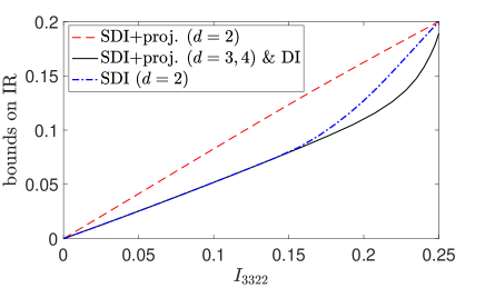
Figure 4: Quantification of incompatibility robustness for given violation of $I_{3322}$. Blue dash-dotted line: SDI approach for $d=2$. Black solid line: DI approach. A similar curve (with a difference of the order of $10^{-5}$) corresponds to the SDI calculation with the additional assumption of projective measurements for $d=3,4$ (identical up to numerical precision). Red dashed line: SDI approach with additional assumption of projective measurements for $d=2$.

VIII Conclusions and outlook

We proposed a framework, the MMM, to quantify the degree of (several notions of) measurement incompatibility in a DI manner. The main idea behind our method is to construct moment matrices by applying a completely positive map on POVMs. Due to the operational characterization of the incompatibility robustness Carmeli et al. (2019); Skrzypczyk et al. (2019); Uola et al. (2019); Takagi et al. (2019); Takagi and Regula (2019); Oszmaniec and Biswas (2019); Mori (2020), our result also bounds, in a DI scheme, the usefulness of a set of POVMs in the problem of quantum state discrimination. In contrast to previous DI bounds of incompatibility in Refs. Cavalcanti and Skrzypczyk (2016); Chen et al. (2016), our method does not rely on any concept of steering, but provides a direct interpretation of the moment matrix as a completely positive mapping of the measurement operators. Our MMM method is shown to outperform both methods in the quantification of incompatibility in simple examples, and we rigorously proven that it always performs better or equal to the method in Ref. Chen et al. (2016). Moreover, the MMM method provides a DI bound of the genuine multipartite incompatibility, a recently introduced notion, for which no DI quantifier was known so far, and it improves the known thresholds for the its detection. Finally, given its generality our method is straightforwardly adaptable to include additional constraints such as the system dimension (semi-DI approach), the assumption of projective measurements, and it is applicable to the prepare-and-measure scenario (see the discussion in App. G).

We leave as an open problem to determine the convergence of the proposed hierarchy. Since we could not give either a positive or negative answer to this question, we used the term “relaxation” for the optimization problems throughout the text. However, we would like to point out that at least in the case of tilted CHSH, for which an analytical solution is known, our method recovers the exact relation between the incompatibility robustness and nonlocality (see Fig. 2).

As a future research direction, we would like to investigate the connection between DI and SDI quantifier of incompatibility and self-testing of measurements (see Ref. Kaniewski et al. (2019) for a related approach). In fact, in Ref. Designolle et al. (2019), the authors showed that for the incompatibility robustness, pairs of measurements associated with mutually unbiased bases (MUBs) are the most incompatible in any dimension, even if it is not proven that they are the only ones. In the CHSH scenario, our calculation showed that $\mathcal{IR_{\rm DI}}$ saturates $\mathcal{IR}$ of a pair of qubit-measurements corresponding to the MUB for the maximal quantum violation of the CHSH inequality (Ref. Chen et al. (2016) also saurates this bound). For high dimensional cases, one can use the family of Bell inequalities in Ref. Tavakoli et al. (2019) to compute $\mathcal{IR_{\rm DI}}$. Due to the limitation of our computational capacity, we leave this issue for the potential future research. This intuition is further strengthened by the work of Ref. Chen et al. (2020), which showed that the assemblage moment matrices proposed in Ref. Chen et al. (2016) can be used to self-test state assemblages. Therefore it is natural to ask if the MMMs can be analogously used to self-test quantum measurements. Finally, a possible further extension of this work is in the direction of the SDI characterization of incompatibility in the prepare-and-measure scenario. In fact, it is believed that incompatible measurements are necessary for quantum advantage in the so-called random access codes Carmeli et al. (2020).

Appendix A Different measures of global incompatibility

In this section, we consider other measures of incompatibility and explicitly write down their DI quantifications in the SDP form. There are robustness-based measures:

$$\mathcal{IR}^{i}:= \min\quad t$$ (16)

$${\rm s.t.} \left\{\frac{{E^{\text{A}}_{a|x}}+t\cdot N_{a|x}}{1+t}\right\}_{a,x}{\rm~{}is~{}jointly~{}measurable},$$

where the noisy models $\{N_{a|x}\}_{a,x}$ satisfy different constraints (see, e.g., Designolle et al. (2019)) and each type of models is denoted by superindices $i$. The last measure we consider is the incompatibility weight Pusey (2015). For the simplicity of formulation of the following SDPs we will not write explicitly the variables of optimization. Instead, we specify the input to each SDP next to “Given”.

A.1 The incompatibility jointly measurable robustness

The noisy assemblage $\{N_{a|x}\}_{a,x}$ for the incompatibility jointly measurable robustness $\mathcal{IR}^{{\tiny\rm J}}$ Cavalcanti and Skrzypczyk (2016) admits a jointly measurable model. As such, $\mathcal{IR}^{{\tiny\rm J}}$ can be computed via the following SDP:

Given $$\{E_{a|x}\}_{a,x}$$ (17)

$$\min \frac{1}{d}\sum_{\lambda}\operatorname{tr}[H_{\lambda}]$$

s.t. $${E^{\text{A}}_{a|x}}=\sum_{\lambda}\delta_{a,\lambda_{x}}(G_{\lambda}-H_{\lambda})\quad\forall a,x,$$

$$G_{\lambda}\succeq 0,\quad H_{\lambda}\succeq 0\quad\forall\lambda,$$

$$\frac{1}{d}\sum_{\lambda}\operatorname{tr}[H_{\lambda}]=\left(\frac{1}{d}\sum_{\lambda}\operatorname{tr}[G_{\lambda}]\right)-1,$$

$$\sum_{\lambda}H_{\lambda}=\left(\frac{1}{d}\sum_{\lambda}\operatorname{tr}[H_{\lambda}]\right)\cdot\openone,$$

$$\sum_{\lambda}G_{\lambda}=\left(\frac{1}{d}\sum_{\lambda}\operatorname{tr}[G_{\lambda}]\right)\cdot\openone.$$

By applying the MMM and removing the constrains containing quadratic free variables, the solution of the following SDP gives a lower bound on $\mathcal{IR}^{{\tiny\rm J}}$:

Given $$P_{\rm obs}(a,b|x,y)$$ (18)

$$\min \sum_{\lambda}\chi[H_{\lambda}]_{\openone}$$

$${\rm s.t.} \chi[{E^{\text{A}}_{a|x}}]=\sum_{\lambda}\delta_{a,\lambda_{x}}\Big{(}\chi[G_{\lambda}]-\chi[H_{\lambda}]\Big{)}$$

$$\chi[G_{\lambda}]\succeq 0,\quad\chi[H_{\lambda}]\succeq 0,\ \ \forall\lambda,$$

$$\sum_{\lambda}\chi[H_{\lambda}]_{\openone}=\left(\sum_{\lambda}\chi[G_{\lambda}]_{\openone}\right)-1,$$

$$\sum_{\lambda}\chi[G_{\lambda}]^{\rm fixed}=\left(\sum_{\lambda}\chi[G_{\lambda}]_{\openone}\right)\cdot\chi[\openone]^{\rm fixed},$$

$$\sum_{\lambda}\chi[H_{\lambda}]^{\rm fixed}=\left(\sum_{\lambda}\chi[H_{\lambda}]_{\openone}\right)\cdot\chi[\openone]^{\rm fixed},$$

$$\sum_{a}\chi[{E^{\text{A}}_{a|x}}]=\chi[\openone],\ \forall x$$

$$\chi[{E^{\text{A}}_{a|x}}]\succeq 0,\ \forall a,x,$$

$$P(a,b|x,y)=P_{\rm obs}(a,b|x,y),\ \forall a,b,x,y,$$

where $\chi[G_{\lambda}]^{\rm fixed}$ and $\chi[H_{\lambda}]^{\rm fixed}$ in the fourth and fifth constraints respectively denote, as in the main text, $\chi[G_{\lambda}]$ and $\chi[H_{\lambda}]$ retaining entries whose indices correspond to non-vanishing terms in $\chi[\openone]^{\rm fixed}$.

A.2 The incompatibility probabilistic robustness

The noisy model for the incompatibility probabilistic robustness $\mathcal{IR}^{{\tiny\rm P}}$ Heinosaari et al. (2014) is defined as $N_{a|x}=p(a|x)\cdot\openone$ for all $a,x,$ with real numbers $p(a|x)$ satisfying $p(a|x)\geq 0$ for all $a,x,$ and $\sum_{a}p(a|x)=1$ for all $x$. The associated SDP can then written as:

Given $$\{E_{a|x}\}_{a,x}$$ (19)

$$\min \left(\frac{1}{d}\sum_{\lambda}\operatorname{tr}[G_{\lambda}]\right)-1$$

s.t. $${E^{\text{A}}_{a|x}}=\sum_{\lambda}\delta_{a,\lambda_{x}}G_{\lambda}-q(a|x)\cdot\openone\quad\forall a,x,$$

$$G_{\lambda}\succeq 0\quad\forall\lambda,\quad q(a|x)\geq 0\quad\forall a,x,$$

$$\sum_{a}q(a|x)=\left(\frac{1}{d}\sum_{\lambda}\operatorname{tr}[G_{\lambda}]\right)-1,$$

$$\sum_{\lambda}G_{\lambda}=\left(\frac{1}{d}\sum_{\lambda}\operatorname{tr}[G_{\lambda}]\right)\cdot\openone.$$

By applying the MMM, a DI lower bound can be computed via the following SDP:

Given $$P_{\rm obs}(a,b|x,y)$$ (20)

$$\min \left(\sum_{\lambda}\chi[G_{\lambda}]_{\openone}\right)-1$$

$${\rm s.t.} \chi[{E^{\text{A}}_{a|x}}]^{\rm fixed}=\sum_{\lambda}\delta_{a,\lambda_{x}}\chi[G_{\lambda}]^{\rm fixed}-q(a|x)\chi[\openone]^{\rm fixed},$$

$$\chi[G_{\lambda}]\succeq 0,\ \forall\lambda,\quad q(a|x)\geq 0,\ \forall a,x,$$

$$\sum_{a}q(a|x)=\left(\sum_{\lambda}\chi[G_{\lambda}]_{\openone}\right)-1$$

$$\sum_{\lambda}\chi[G_{\lambda}]^{\rm fixed}=\left(\sum_{\lambda}\chi[G_{\lambda}]_{\openone}\right)\cdot\chi[\openone]^{\rm fixed},$$

$$\sum_{a}\chi[{E^{\text{A}}_{a|x}}]=\chi[\openone^{\rm A}],\ \forall x,$$

$$\chi[{E^{\text{A}}_{a|x}}]\succeq 0,\ \forall a,x,$$

$$P(a,b|x,y)=P_{\rm obs}(a,b|x,y)\ \forall a,b,x,y.$$

A.3 The incompatibility random robustness

The final robustness-based measure is the incompatibility random robustness $\mathcal{IR}^{{\tiny\rm R}}$ Heinosaari et al. (2015); Uola et al. (2015), where the noisy assemblage is composed of the white noise: $N_{a|x}=(1/|\mathcal{A}|)\cdot\openone$. As a result, the corresponding SDP is given by

Given $$\{E_{a|x}\}_{a,x}$$ (21)

$$\min \left(\frac{1}{d}\sum_{\lambda}\operatorname{tr}[G_{\lambda}]\right)-1$$

s.t. $${E^{\text{A}}_{a|x}}=\sum_{\lambda}\delta_{a,\lambda_{x}}G_{\lambda}-\frac{1}{|\mathcal{A}|}\left(\Big{(}\frac{1}{d}\sum_{\lambda}\operatorname{tr}[G_{\lambda}]\Big{)}-1\right)\cdot\openone,$$

$$G_{\lambda}\succeq 0,\ \forall\lambda,$$

$$\sum_{\lambda}G_{\lambda}=\left(\frac{1}{d}\sum_{\lambda}\operatorname{tr}[G_{\lambda}]\right)\cdot\openone.$$

With the same technique, a DI lower bound on $\mathcal{IR}^{{\tiny\rm R}}$ can be computed via the following SDP:

Given $$P_{\rm obs}(a,b|x,y)$$ (22)

$$\min \left(\sum_{\lambda}\chi[G_{\lambda}]_{\openone}\right)-1$$

$${\rm s.t.} \chi[{E^{\text{A}}_{a|x}}]^{\rm fixed}=\sum_{\lambda}\delta_{a,\lambda_{x}}\chi[G_{\lambda}]^{\rm fixed}$$

$$\quad\quad\quad\quad\quad\quad-\frac{1}{|\mathcal{A}|}\left(\sum_{\lambda}\chi[G_{\lambda}]_{\openone}-1\right)\cdot\chi[\openone]^{\rm fixed},$$

$$\sum_{\lambda}\chi[G_{\lambda}]^{\rm fixed}=\left(\sum_{\lambda}\chi[G_{\lambda}]_{\openone}\right)\cdot\chi[\openone]^{\rm fixed},$$

$$\sum_{a}\chi[{E^{\text{A}}_{a|x}}]=\chi[\openone^{\rm A}],\ \forall x,$$

$$\chi[G_{\lambda}]\succeq 0,\ \forall\lambda,$$

$$\chi[{E^{\text{A}}_{a|x}}]\succeq 0,\ \forall a,x,$$

$$P(a,b|x,y)=P_{\rm obs}(a,b|x,y),\ \forall a,b,x,y.$$

A.4 The incompatibility weight

The last measure of incompatibility we consider is the incompatibility weight $\mathcal{IW}$ Pusey (2015). Consider that one decomposes ${E^{\text{A}}_{a|x}}$ into ${E^{\text{A}}_{a|x}}=tO_{a|x}+(1-t)N_{a|x}$, where $\{O_{a|x}\}_{a,x}$ is any valid quantum measurement assemblage and $\{N_{a|x}\}_{a,x}$ is a jointly measurable measurement assemblage. $\mathcal{IW}$ is defined as the minimum ratio of $O_{a|x}$, i.e., the minimum value of $t$, required to decompose ${E^{\text{A}}_{a|x}}$. Consequently, $\mathcal{IW}$ can be computed via the following SDP:

Given $$\{E_{a|x}\}_{a,x}$$ (23)

$$\min 1-\frac{1}{d}\sum_{\lambda}\operatorname{tr}[G_{\lambda}]$$

$${\rm s.t.} {E^{\text{A}}_{a|x}}\succeq\sum_{\lambda}\delta_{a,\lambda_{x}}G_{\lambda}\quad\forall a,x,$$

$$G_{\lambda}\succeq 0\quad\forall\lambda,$$

$$\sum_{\lambda}G_{\lambda}=\frac{1}{d}\left(\sum_{\lambda}\operatorname{tr}[G_{\lambda}]\right)\cdot\openone,$$

Following the same procedure as in the previous sections, we obtain the following SDP, which can be used to compute a DI lower bound on $\mathcal{IW}$:

Given $$P_{\rm obs}(a,b|x,y)$$ (24)

$$\min 1-\sum_{\lambda}\chi[G_{\lambda}]_{\openone}$$

$${\rm s.t.} \chi[{E^{\text{A}}_{a|x}}]\ \succeq\sum_{\lambda}\delta_{a,\lambda_{x}}\chi[G_{\lambda}],\$$

$$\chi[G_{\lambda}]\succeq 0,\ \forall\lambda,$$

$$\sum_{\lambda}\chi[G_{\lambda}]^{\rm fixed}=\sum_{\lambda}\chi[G_{\lambda}]_{\openone}\cdot\chi[\openone]^{\rm fixed},$$

$$\sum_{a}\chi[{E^{\text{A}}_{a|x}}]=\chi[\openone],\ \forall x,$$

$$\chi[{E^{\text{A}}_{a|x}}]\succeq 0,\ \forall a,x,$$

$$P(a,b|x,y)=P_{\rm obs}(a,b|x,y),\ \forall a,b,x,y.$$

Note that all of above SDPs that compute DI lower bounds on the degree of incompatibility require the detailed information about the observed correlation $\{P_{\rm obs}(a,b|x,y)\}_{a,b,x,y}$. If one is merely concerned with a Bell inequality violation without the specific characterization of $\{P_{\rm obs}(a,b|x,y)\}_{a,b,x,y}$, the constrains containing $\chi[\openone]^{\rm fixed}$ have to be fully removed.

Appendix B Different constraints on incompatibility robustness

As we discussed in the main text, different relaxations of the following problem exist

$$\min_{\{\chi[G_{\lambda}],\chi[E_{a|x}]\}_{\lambda,a,x}} \sum_{\lambda}\chi[G_{\lambda}]_{\openone}-1$$ (25)

$${\rm s.t.} \sum_{\lambda}\delta_{a,\lambda_{x}}\chi[G_{\lambda}]\ \succeq\chi[{E^{\text{A}}_{a|x}}]\quad\forall a,x,$$

$$\chi[G_{\lambda}]\succeq 0\quad\forall\lambda,$$

$$\sum_{\lambda}\chi[G_{\lambda}]=\sum_{\lambda}\chi[G_{\lambda}]_{\openone}\cdot\chi[\openone],$$

$$\sum_{a}\chi[{E^{\text{A}}_{a|x}}]=\chi[\openone]\quad\forall x,$$

$$\chi[{E^{\text{A}}_{a|x}}]\succeq 0\quad\forall a,x,$$

$$P(a,b|x,y)=P_{\rm obs}(a,b|x,y)\quad\forall a,b,x,y,$$

which are necessary to remove the nonlinear constraint: $\sum_{\lambda}\chi[G_{\lambda}]=\sum_{\lambda}\chi[G_{\lambda}]_{\openone}\cdot\chi[\openone]$. Moreover, the problem in Eq. (25) assume the knowledge of the full distribution of probabilities $\{P_{\rm obs}(a,b|x,y)\}_{a,b,x,y}$, whereas in some cases, we may want to estimate the robustness simply from the violation of a Bell inequality.

In this case, we want to characterize the set of all possible pairs $(\mathcal{IR},I(P))$, where $\mathcal{IR}$ represents the incompatibility robustness and $I(P)$ the value of some Bell expression. Notice that, even if $I(P)$ is evaluated on a probability distribution $P$, we are not assuming that such $P$ is directly accessible, the parameter in our problem is only the value of the Bell expression.

The set of valid $(\mathcal{IR},I(P))$ can be defined by the following SDP (feasibility problem):

Given $$\mathcal{IR}_{0},\ I(P_{0})$$ (26)

find $$\chi[\openone],\chi[G_{\lambda}],\chi[E_{a|x}]$$

$${\rm s.t.} \sum_{\lambda}\delta_{a,\lambda_{x}}\chi[G_{\lambda}]\ \succeq\chi[{E^{\text{A}}_{a|x}}]\quad\forall a,x,$$

$$\chi[G_{\lambda}]\succeq 0\quad\forall\lambda,$$

$$\sum_{a}\chi[{E^{\text{A}}_{a|x}}]=\chi[\openone]\quad\forall x,$$

$$\chi[{E^{\text{A}}_{a|x}}]\succeq 0\quad\forall a,x,$$

$$\sum_{\lambda}\chi[G_{\lambda}]_{\openone}=\mathcal{IR}_{0}+1,$$

$$I(P_{0})=\sum_{a,x}\alpha_{a,x}\operatorname{tr}\left[\chi[{E^{\text{A}}_{a|x}}]\ W_{a,x}\right],$$

where the matrices $W_{a,x}$ and the coefficients $\alpha_{a,x}$ are properly chosen to extract the Bell expression from the terms corresponding to probabilities appearing in $\{\chi[{E^{\text{A}}_{a|x}}]\}_{a,x}$. It is then clear, then, the (nontrivial) extreme points of this set are equivalently characterized by the following two problems:

$$\begin{split}&\text{ minimize }\mathcal{IR}\text{ given }I(P),\quad\text{ and }\\ &\text{ maximize }I(P)\text{ given }\mathcal{IR}.\end{split}$$ (27)

In fact, one may have highly incompatible observables and fail to obtain a highly violation of a Bell inequality due to the low entanglement in the shared state. The problems in Eq. (27) can be directly solved by transforming the feasibility problem in Eq. (26). By construction, a feasible solution of one problem is also a feasible solution for the other one, so they characterize the same set of pairs $(\mathcal{IR},I(P))$. It is important to remark that here we are not using the full duality properties of the SDP, but simply the relation between $\mathcal{IR}$ and $I(P)$ encoded in Eq. (26) and the fact that the problems in Eq. (27) are sufficient to characterize the nontrivial part of this set.

The formulation with the fixed $\mathcal{IR}_{0}$, however, provides an advantage since an extra condition can be imposed. In fact, the substitution $\sum_{\lambda}\chi[G_{\lambda}]_{\openone}-1=\mathcal{IR}_{0}$, allows us to write the third constraint of Eq. (25) as $\sum_{\lambda}\chi[G_{\lambda}]=(\mathcal{IR}_{0}+1)\chi[\openone]$, effectively removing the nonlinearity appearing in the SDP in Eq. (25). We then have

Given $$\mathcal{IR}_{0}$$ (28)

$$\max_{\chi[\openone],\{\chi[G_{\lambda}],\chi[E_{a|x}]\}_{\lambda,a,x}} I(P)=\sum_{a,x}\alpha_{a,x}\operatorname{tr}\left[\chi[{E^{\text{A}}_{a|x}}]\ W_{a,x}\right]$$

$${\rm s.t.} \sum_{\lambda}\delta_{a,\lambda_{x}}\chi[G_{\lambda}]\ \succeq\chi[{E^{\text{A}}_{a|x}}]\quad\forall a,x,$$

$$\chi[G_{\lambda}]\succeq 0\quad\forall\lambda,$$

$$\sum_{\lambda}\chi[G_{\lambda}]=(\mathcal{IR}_{0}+1)\chi[\openone],$$

$$\sum_{a}\chi[{E^{\text{A}}_{a|x}}]=\chi[\openone]\quad\forall x,$$

$$\chi[{E^{\text{A}}_{a|x}}]\succeq 0\quad\forall a,x,$$

$$\sum_{\lambda}\chi[G_{\lambda}]_{\openone}=\mathcal{IR}_{0}+1,$$

The fact that the SDP in Eq. (28) provides a better characterization of the set $(\mathcal{IR},I(P))$ is confirmed by numerical calculations. First, the incompatibility robustness has been analyzed in Fig. 2, where this distinction is not relevant. However, a characterization analogous to that in Eq. (27) appears also for the genuine multipartite incompatibility robustness. For that case, we can see directly that the use of the two different formulations provides different results and that the computation for a fixed robustness $\mathcal{IR}_{0}$ provides a better bound. More details can be found in App. C.

Appendix C SDP formulation for genuine-multipartite incompatibility

In the following, we recall several results from Ref. Quintino et al. (2019), in particular the SDPs (30) and (C), and discuss their DI relaxation via the MMM.

Following Quintino et al. (2019), we recall that genuine triplewise incompatibility , namely, the impossibility of writing

$$E_{a|x}=p_{12}J^{12}_{a|x}+p_{23}J^{23}_{a|x}+p_{13}J^{13}_{a|x}$$ (29)

for some probabilities $p_{12}$, $p_{23}$, and $p_{13}$ with $p_{12}+p_{23}+p_{13}=1$, is equivalent to the infeasibility of the following SDP:

Given $$\quad\{E_{a|1}\}_{a},\{E_{a|2}\}_{a},\{E_{a|3}\}_{a}$$ (30)

find $$\quad J^{12}_{a|x}\ ,\;J^{23}_{a|x}\ ,\;J^{31}_{a|x}\ ,\;p_{12},\;p_{23},\;p_{31},\;G^{12}_{\lambda},\;G^{23}_{\lambda},\;G^{31}_{\lambda}$$

s.t. $$\quad G_{\lambda}^{12},G_{\lambda}^{23},G_{\lambda}^{13}\succeq 0,\;\;p_{12},p_{23},p_{13}\geq 0,$$

$$\quad E_{a|x}=J^{12}_{a|x}+J^{23}_{a|x}+J^{13}_{a|x}\ ,\ \forall a,x,$$

$$\quad J^{12}_{a|x}\succeq 0,\;\forall a,x;\;\sum_{a}J^{12}_{a|x}=p_{12}\openone,\;\forall x,$$

$$\quad J^{12}_{a|x}=\sum_{\lambda}\delta_{a,\lambda_{x}}G^{12}_{\lambda}\quad\text{ for }x=1,x=2,$$

$$\quad J^{23}_{a|x}\succeq 0,\;\forall a,x;\;\sum_{a}J^{23}_{a|x}=p_{23}\openone,\;\forall x,\;$$

$$\quad J^{23}_{a|x}=\sum_{\lambda}\delta_{a,\lambda_{x}}G^{23}_{\lambda}\quad\text{ for }x=2,x=3,$$

$$\quad J^{13}_{a|x}\succeq 0,\;\forall a,x;\;\sum_{a}J^{13}_{a|x}=p_{13}\openone,\;\forall x,$$

$$\quad J^{13}_{a|x}=\sum_{\lambda}\delta_{a,\lambda_{x}}G^{13}_{\lambda}\quad\text{ for }x=1,x=3,$$

where $\delta_{a,\lambda_{x}}$ is the deterministic strategy that assign probability $1$ if the $x$-th component of $\lambda$ is equal to $a$.

One can quantify the triplewise incompatibility of a set of measurements using SDP methods. We need few definitions and properties: $J^{3}_{a|x}:=J^{sx}_{a|x}+J^{tx}_{a|x}+J^{st}_{a|x}$ , for $x=1,2,3$ and $s,t,x$ all different. When $\{J_{a|x}^{12},J_{a|x}^{13},J_{a|x}^{23}\}_{a,x}$ is a solution of the problem in Eq. (30), we have that $J^{sx}_{a|x}$ and $J^{tx}_{a|x}$ arise each from a joint measurement, $J^{st}_{a|x}$ is positive, $\{G_{\lambda}^{st}\}$ is proportional to a POVM with the same proportionality constant as $\{J^{st}_{a|x}\}_{a}$ for all $x$, i.e., $\sum_{a}J^{st}_{a|x}=\sum_{\lambda}G^{st}_{\lambda}$ for all $s,t,x$. Finally, both $\{J^{3}_{a|x}\}_{a}$ and $\{G^{12}_{\lambda}+G^{13}_{\lambda}+G^{23}_{\lambda}\}$ are POVMs. From the above formulation, we can define a robustness with respect to arbitrary noise as

$$\begin{split}t^{*}=\min\left\{\ t\ \middle|J^{3}_{a|x}=\frac{E_{a|x}+tN_{a|x}}{1+t},\text{ for }\{J^{3}_{a|x}\}\text{ sol.\ of}\text{ ~{}\eqref{SDP_GMI}, }\right.\\ \left.\{N_{a|x}\}\text{ meas. assemb. }\right\}\end{split}$$ (31)

Following the argument in Ref. Quintino et al. (2019), one shows that $t*$ can be computed as

Given $$\{E_{a|x}\}_{a,x},$$

and variables $$\{G^{12}_{\lambda},G^{13}_{\lambda},G^{23}_{\lambda}\}_{\lambda},\{J_{a|3}^{12},J_{a|2}^{13},J_{a|1}^{23}\}_{a},$$

$$\min\ \frac{1}{d}\sum_{\lambda}\operatorname{tr}[G^{12}_{\lambda}+G^{13}_{\lambda}+G^{23}_{\lambda}]-1$$ (32)

s.t. $$G^{st}_{\lambda}\succeq 0\ \forall\lambda,\ \sum_{\lambda}G^{st}_{\lambda}=\frac{\openone}{d}\sum_{\lambda}\operatorname{tr}[G^{st}_{\lambda}]$$

$$\text{ for }(s,t)=(1,2),(1,3),(2,3);$$

$$J^{st}_{a|x}\succeq 0,\ \forall a,\ \sum_{a}J^{st}_{a|x}=\sum_{\lambda}G^{st}_{\lambda}\text{ and }$$

$$\sum_{\lambda}\delta_{a,\lambda_{x}}(G^{sx}_{\lambda}+G^{tx}_{\lambda})+J^{st}_{a|x}\succeq E_{a|x},$$

$$\text{ for }(s,t,x)=(1,2,3),(1,3,2),(2,3,1);$$

to show the strict feasibility, implying via Slater’s conditon that the primal and the dual problem have the same optimal values, it is sufficient to take each $G^{st}_{\lambda}=\openone$ and the corresponding $J^{st}_{a|x}$ coming from the linear constraints.

Clearly, the same argument can be extended to define genuine multipartite incompatibility beyond the triplewise case.

Finally, we can show that the SDP computing the maximum of a Bell inequality $I(P)$ for a given robustness $\mathcal{IR}_{0}$, namely,

Given: $$\mathcal{IR}_{0},\text{ and }$$

variables: $$\{\chi[E_{a|x}]\}_{a,x},\text{ and }\{\chi[G^{st}_{\lambda}]\}_{\lambda},\{\chi[J^{st}_{a|x}]\}_{a},$$

$$\text{ for }(s,t,x)=(1,2,3),(1,3,2),(2,3,1),$$

$$\max\ I(P)$$

s.t. $$\chi[G^{st}_{\lambda}]\succeq 0\ \forall\lambda,(s,t)=(1,2),(1,3),(2,3);$$

$$\sum_{\lambda,(s,t)}\chi[G^{st}_{\lambda}]=\chi[\openone](\mathcal{IR}_{0}+1)\ \text{ and }$$

$$\sum_{\lambda,(s,t)}\chi[G^{st}_{\lambda}]_{\openone}=(\mathcal{IR}_{0}+1),$$

$$\text{ with sum over }(s,t)=(1,2),(1,3),(2,3);$$

$$\chi[J^{st}_{a|x}]\succeq 0,\ \forall a,\ \sum_{a}\chi[J^{st}_{a|x}]=\sum_{\lambda}\chi[G^{st}_{\lambda}]\text{ and }$$

$$\sum_{\lambda}\delta_{a,\lambda_{x}}(\chi[G^{sx}_{\lambda}]+\chi[G^{tx}_{\lambda}])+\chi[J^{st}_{a|x}]\succeq\chi[E_{a|x}],$$

$$\text{ for }(s,t,x)=(1,2,3),(1,3,2),(2,3,1);$$

$$\chi[E_{a|x}]\succeq 0,\text{ for all }a,x,$$

$$\sum_{a}\chi[E_{a|x}]=\chi[\openone],\text{ for all }x,$$ (33)

provides a better bound with respect to similar SDP computing the minimal robustness $\mathcal{IR}$ for a given Bell violation $I(P_{0})$. More details can be found in Fig. 5.

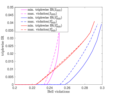
Figure 5: Comparison between two SDPs computing the bounds. The solid curves are bounds obtained by fixing a Bell violation and minimizing the robustness (cf. Eq. (VI)) while the dashed curves are bounds obtained by fixing a robustness and maximizing the Bell violation (cf. Eq. (C)).

Appendix D Witnesses of genuine-multipartite incompatibility

To make our discuss self-contained, we briefly recall in this section two witnesses of GMI presented in Ref. Quintino et al. (2019). To keep the notation lighter, we will discuss only the case of genuine tripartite incompatibility; the argument can then be generalized to more measurements.

The authors of Ref. Quintino et al. (2019) define the set $L_{12}^{Q}$ as the set of bipartite correlations with three measurements for Alice, in which the pair $x=1,2$ is compatible (one should specify also Bob’s settings and outcomes, i.e., the whole Bell scenario). Given three measurement $\{\{E_{a|x}\}_{a}\}_{x=1,2,3}$ we say that

$$P(ab|xy)\text{ belongs to }L_{12}^{Q}\text{ if: }$$

$$P(ab|xy)\in\mathcal{Q},$$

$$\{\{P(ab|xy)\}_{a,b,y}\}_{x=1,2}\text{ is local }.$$ (34)

For the set of quantum correlations $\mathcal{Q}$, typically only an approximate characterization is possible, namely, via the NPA hierarchy of a given level $l$.

In particular, for the case of Alice having only dichotomic outcomes, the condition that $\{\{P(ab|xy)\}_{a,b,y}\}_{x=1,2}$ is local can be simply imposed by requiring that all CHSH inequalities for Alice’s pair of measurements and all possible pairs of dichotomized measurements for Bob are satisfied Pironio (2014), namely

$$P(ab|xy)\text{ belongs to }L_{12}^{Q}\text{ if: }$$

$$P(ab|xy)\in\mathcal{Q},$$

$$\{\{P(ab|xy)\}_{a,b,y}\}_{x=1,2}\text{ satisfies CHSH for any }$$ (35)

$$\text{ pair of dichotomized measurements for Bob}.$$

In simple terms, this set is obtained by the NPA-hierarchy constraints plus linear constraints corresponding to Bell inequalities involving only $x=1,2$ and all possible dichotomized measurements on Bob’s side.

The above definition can be extended to the convex hull of $L_{12},L_{13},L_{23}$, i.e., $L_{2{\rm conv}}$ as follows

$$P(ab|xy)\text{ belongs to }L_{2{\rm conv}}^{Q}\text{ if: }$$

$$P(ab|xy)\in\mathcal{Q},$$

$$P(ab|xy)=\mu_{12}P_{12}(ab|xy)+\mu_{13}P_{13}(ab|xy)+\mu_{23}P_{23}(ab|xy),$$

$$P_{ij}(ab|xy)\in L^{Q}_{ij},\ \mu_{ij}\geq 0,\ \mu_{12}+\mu_{13}+\mu_{23}=1$$ (36)

As noticed in Ref. Quintino et al. (2019), imposing locality constraints at the level of the observed distribution is not the same as imposing constraints on the joint measurability of observables in the NPA hierarchy approximating the set $Q$. For instance, consider the set $Q_{12_{JM}}$ defined as follow

$$P(ab|xy)\text{ belongs to }Q_{12_{JM}}\text{ if: }$$

$$P(ab|xy)\in\mathcal{Q},\text{ with }$$

$$E_{a|1}=\sum_{a^{\prime}}M_{aa^{\prime}}^{12},\ \forall a,\ E_{a^{\prime}|2}=\sum_{a}M_{aa^{\prime}}^{12},\forall a^{\prime}.$$ (37)

In other words, the two measurements $\{E_{a|1}\}_{a}$ and $\{E_{a|2}\}_{a}$ are substituted by a single joint measurement $M_{aa^{\prime}}^{12}$. In terms of the NPA hierarchy, this can be simply obtained by taking the moments involving $M_{aa^{\prime}}^{12}$ instead of $\{E_{a|1}\}_{a}$ and $\{E_{a|2}\}_{a}$. Similarly, the convex hull $Q_{2{\rm conv}_{JM}}$ can be defined as

$$P(ab|xy)\text{ belongs to }Q_{2{\rm conv}_{JM}}\text{ if: }$$

$$P(ab|xy)\in\mathcal{Q},$$

$$P(ab|xy)=\mu_{12}P_{12}(ab|xy)+\mu_{13}P_{13}(ab|xy)+\mu_{23}P_{23}(ab|xy),$$

$$P_{ij}(ab|xy)\in Q_{ij_{JM}},\ \mu_{ij}\geq 0,\ \mu_{12}+\mu_{13}+\mu_{23}=1.$$ (39)

The SDP approximation of this set involves computing three different NPA moment matrices, one for each distribution $P_{ij}(ab|xy)$.

It is important to remark that the NPA hierarchy can be computed by assuming the dilation of the POVMs to projective measurements. It is also important to remark that, even if some structure of measurement incompatibility require POVMs (e.g., the hollow triangle), in Eq. (D) only pairwise JM conditions arise, one for each $P_{ij}$. A total JM measurability condition among a measurement assemblage $\{E_{a|x}\}_{a,x}$ is equivalent to the existence of a common dilation in which the measurements are represented by commuting projective measurements. In this sense, due to the convex nature of the genuine multipartite incompatibility problem, there is no contradiction between the use of the dilation and the fact that non-trivial compatibility structures necessarily require POVMs.

Appendix E Relation between the measurement moment matrix and the assemblage moment matrix

The assemblage moment matrices proposed in Ref. Chen et al. (2016) can be viewed as a special case of the MMM, as we show below. If the sequence $\{S_{i}\}$ in Eq. (5) of the main text is only composed of Bob’s projectors and their products, namely, $\{S_{i}\}=\{\openone\otimes B_{i}\}$ with $\{B_{i}\}=\{\openone,E_{1|1}^{\rm B},E_{2|1}^{\rm B},E_{1|1}^{\rm B}E_{1|2}^{\rm B},{\rm etc}...\}$, then Eq. (5) of the main text will be

$$\chi=\sum_{ij}|i\rangle\langle j|\operatorname{tr}(B_{j}^{\dagger}B_{i}\sigma_{a|x}),$$ (40)

with $\sigma_{a|x}:=\operatorname{tr}_{\rm A}({E^{\text{A}}_{a|x}}\otimes\openone^{\rm B}{\varrho^{\text{AB}}})$ being the state assemblage in a steering-type experiment, which recovers the form of the assemblage moment matrices. Moreover, since each constraint in the SDP for computing the bounds in Ref. Chen et al. (2016) is also a constraint of the SDP derived from Eq. (7) in the main text, but not vice versa, the MMM bounds will never be worse than those in Ref. Chen et al. (2016). In Ref. Chen et al. (2018), the authors further obtained tighter DI bounds on $\mathcal{IR}$ by bounding another measure of steerability — the consistent steering robustness, which is also a lower bound on $\mathcal{IR}$ Cavalcanti and Skrzypczyk (2016). If we consider again that the sequence $\{S_{i}\}$ is only composed of Bob’s part, the only difference between the SDP derived from Eq. (7) in the main text and the SDP used for bounding the consistent steering robustness in Ref. Chen et al. (2018) is that the latter does not include the fourth constraint of the former: $\sum_{a}\chi[{E^{\text{A}}_{a|x}}]=\chi[\openone]$. As a consequence, the present DI bound on $\mathcal{IR}$ will not be lower than that of Ref. Chen et al. (2018).

Finally, by computing explicitly the $\mathcal{IR}$ bounds associated with a given violation of the $I_{3322}$ inequality and provided, respectively, by the method in Ref. Chen et al. (2016) and by the MMM method, we show that the MMM method provides a tighter value. The results of numerical calculations are plotted in Fig. 6.

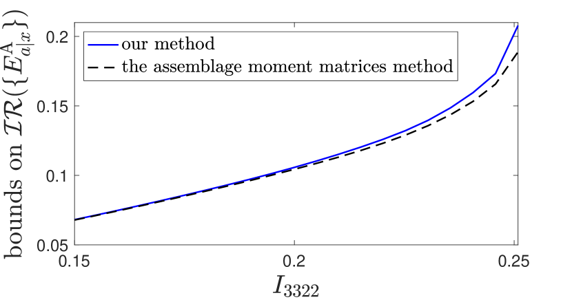
Figure 6: Comparison between lower bounds on $\mathcal{IR}$ in the $I_{3322}$ scenario Collins and Gisin (2004). The blue-solid and black-dashed curves represent, respectively, lower bounds obtained from our method and from the method of the assemblage moment matrices Chen et al. (2016). The local and quantum bounds for the $I_{3322}$ inequality are, respectively, $0$ and around $0.250875561$ Rosset (2018). The levels of the hierarchy of the semidefinite relaxation used to carry out the computation in both methods are the $3$rd level.

Appendix F POVMs and projective measurements in the SDI scenario

Projective measurements, via their idempotence and orthogonality properties ($P_{a}P_{b}=P_{a}\delta_{a,b}$), allow for a great simplification of the sequences appearing in the construction of moment matrices. In the DI scenario, all measurements can be assumed to be projective due to the Neumark dilation, as discussed in the main text. Such a dilation, however, requires to increase the Hilbert space dimension and is, thus, not always possible if the dimension of the system is constrained as in the SDI scenario. In some cases, however, projective measurements can be recovered by a convexity argument. For instance, for dichotomic measurements, it is known that they are all convex mixtures of projective measurements (intuitively, it is sufficient to decompose the $0$-outcome element), so we can restrict ourselves to projective measurements if the objective function we wish to minimize is linear in the POVMs operator. This is the case for, e.g., Bell inequalities as noted in Navascués and Vértesi (2015), but it is also the case for the incompatibility robustness. In order to show that, it is useful to introduce first some slack variables ($\{S_{a,x}\}_{a,x}$), namely,

$$\mathcal{IR}+1=\min_{\{G_{\lambda}\}} \frac{1}{d}\sum_{\lambda}\operatorname{tr}[G_{\lambda}]$$ (41)

$${\rm s.t.} \ \sum_{\lambda}\delta_{a,\lambda_{x}}G_{\lambda}+S_{a,x}={E^{\text{A}}_{a|x}}\ \forall\ a,x,\$$

$$G_{\lambda}\succeq 0,\ S_{a,x}\succeq 0,\ \forall\ \lambda,a,x,\$$

$$\sum_{\lambda}G_{\lambda}-\frac{1}{d}\left(\sum_{\lambda}\operatorname{tr}[G_{\lambda}]\right)\cdot\openone=0,$$

to put the problem in the standard form

$$\min_{X} \langle C,X\rangle$$ (42)

$${\rm s.t.} \langle A_{k},X\rangle=b_{k},\forall\ k$$

$$X\succeq 0.$$

It is then clear that the entries of the POVM elements $E_{a|x}$ will appear in the vector $b$, and consequently in the objective of the dual problem

$$\max_{y} \langle b,y\rangle$$ (43)

$${\rm s.t.} \sum_{k}y_{k}A_{k}\preceq C.$$

It is clear that if, for a given $x$, $E_{a|x}=\sum_{i}\mu_{i}P_{a|x}^{i}$, the minimal robustness will be obtained for a given projective measurement $\{P^{i}_{a|x}\}_{a,x}$.

It is not obvious, however, what happens if one tries to minimize the robustness for a fixed Bell inequality violation. In fact, by choosing one element of the decomposition as above, we may decrease both the robustness and the Bell inequality violation.

A possible approach to the problem by dilation of the measurements of both Alice and Bob, has been already proposed in Ref. Navascués and Vértesi (2015), while generating a basis for $\mathcal{S}_{d}$, the space of moment matrices corresponding to dimension $d$, one should sample Alice’s and Bob’s measurements of the form

$${E^{\text{A}}_{a|x}}=U^{x}(|a\rangle\langle a|_{A^{\prime}}\otimes\openone_{A})(U^{x})^{\dagger},$$

$${E^{\text{B}}_{b|y}}=U^{y}(|b\rangle\langle b|_{B^{\prime}}\otimes\openone_{B})(U^{y})^{\dagger},$$ (44)

with random unitaries $U^{x}$ and $U^{y}$. Random states should then be taken of the form $\rho=|0\rangle\langle 0|_{A^{\prime}}\otimes|0\rangle\langle 0|_{B^{\prime}}\otimes|\psi\rangle\langle\psi|_{AB}$. Since we are interested in dichotomic measurements, dimension of the auxiliary spaces $A^{\prime}$ and $B^{\prime}$ is $2$ in both cases. In practice, however, this method was not able to provide a better bound of the SDI bound in $d=2$ for the $I_{3322}$ inequality.

Appendix G Extension of MMM method to the prepare-and-measure scenario

The prepare-and-measure (P-M) scenario, e.g., the one given by random access codes Pawłowski and Brunner (2011); Carmeli et al. (2020), is a paradigm often considered in quantum information processing as an alternative to the Bell scenario. The P-M scenario is a one-way communication scenario in which one party, let us say Bob, prepares a physical system in a state $\rho_{y}$ chosen from a finite set indexed by $y$ and sends it to the other party, Alice. Alice measures this system with a choice of measurement specified by $x$. The conditional distribution $P(a|x,y)$, where $a$ is the outcome of Alice’s measurement, is then used to semi-device-independently characterize the states and measurements in this scenario. The classical distribution $P(a|x,y)$ is the one produced by states and measurements which can be simultaneously diagonalized in some basis of the Hilbert space in which they are defined.

One important distinction between the P-M and Bell scenario is that parties’ measurements do not need to be space-like separated. However, in order to observe a gap between classical and quantum strategies some form of restriction on the communication needs to be imposed Hoffmann et al. (2018); Budroni et al. (2019). Here, we consider the most common type of restriction, an upper-bound on the Hilbert’s space dimension in which the states and measurements are defined. This enables us to use the hierarchy of Ref. Navascués and Vértesi (2015) to approximate the set of quantum correlations $P(a|x,y)$ and subsequently map the incompatibility robustness SDP to MMM SDP.

The map is a direct extension, merely a simplification of Eq. (4) of the main text, and can be written as follows:

$$\chi[{E^{\text{A}}_{a|x}}]:=\sum_{n}K_{n}({E^{\text{A}}_{a|x}})K_{n}^{\dagger}\quad\forall a,x,$$ (45)

where $K_{n}:=\sum_{i}|i\rangle_{\overline{\rm A}{\rm A}}\langle n|S_{i}$, and $\{S_{i}\}$ is the following sequence of operators: $\{S_{i}\}=\{\openone^{\rm A},{E^{\text{A}}_{a|x}},\rho_{y},{E^{\text{A}}_{a|x}}\rho_{y},{\rm etc.}\}$. The MMM can then be defined as

$$\chi_{\{S_{i}\}}[{E^{\text{A}}_{a|x}}]=\sum_{ij}|i\rangle\langle j|\operatorname{tr}\left[S_{i}({E^{\text{A}}_{a|x}})S_{j}^{\dagger}\right],$$ (46)

which is a direct analogy of Eq. (5) of the main text. Using this map, one can formulate an SDI relaxation of incompatibility robustness SDP, which reads

$$\min_{\{\chi[G_{\lambda}],\chi[E_{a|x}]\}_{\lambda,a,x}} \sum_{\lambda}\chi[G_{\lambda}]_{\openone}-1$$ (47)

$${\rm s.t.} \sum_{\lambda}\delta_{a,\lambda_{x}}\chi[G_{\lambda}]\ \succeq\chi[{E^{\text{A}}_{a|x}}]\quad\forall a,x,$$

$$\chi[G_{\lambda}]\succeq 0\quad\forall\lambda,$$

$$\sum_{\lambda}\chi[G_{\lambda}]=\sum_{\lambda}\chi[G_{\lambda}]_{\openone}\cdot\chi[\openone],$$

$$\sum_{a}\chi[{E^{\text{A}}_{a|x}}]=\chi[\openone]\quad\forall x,$$

$$\chi[{E^{\text{A}}_{a|x}}]\succeq 0\quad\forall a,x,$$

$$\chi[{E^{\text{A}}_{a|x}}]\in\mathcal{S}_{d},\quad\forall a,x,$$

$$\chi[\openone]\in\mathcal{S}_{d},$$

$$P(a|x,y)=P_{\rm obs}(a|x,y)\quad\forall a,x,y,$$

where $\mathcal{S}_{d}$ is a subspace of moment matrices spanned by those corresponding to states and measurements defined on Hilbert space of dimension $d$.

References

- Heisenberg (1927) W. Heisenberg, “Über den anschaulichen inhalt der quantentheoretischen kinematik und mechanik,” Z. Physik , 172––198 (1927).
- Robertson (1929) H. P. Robertson, “The uncertainty principle,” Phys. Rev. 34, 163–164 (1929).
- Busch et al. (2014) P. Busch, P. Lahti, and R. F. Werner, “Colloquium : Quantum root-mean-square error and measurement uncertainty relations,” Rev. Mod. Phys. 86, 1261–1281 (2014).
- Bell (1964) J. S. Bell, “On the Einstein Podolsky Rosen paradox,” Physics Physique Fizika 1, 195–200 (1964).
- Brunner et al. (2014) N. Brunner, D. Cavalcanti, S. Pironio, V. Scarani, and S. Wehner, “Bell nonlocality,” Rev. Mod. Phys. 86, 419–478 (2014).
- Schrödinger (1935) E. Schrödinger, “Discussion of probability relations between separated systems,” Proc. Cambridge Phil. Soc. 31, 555 (1935).
- Cavalcanti and Skrzypczyk (2017) D. Cavalcanti and P. Skrzypczyk, “Quantum steering: a review with focus on semidefinite programming,” Reports on Progress in Physics 80, 024001 (2017).
- Uola et al. (2020) R. Uola, A. C. S. Costa, H. C. Nguyen, and O. Gühne, “Quantum steering,” Rev. Mod. Phys. 92, 015001 (2020).
- Kochen and Specker (1967) S. Kochen and E. Specker, “The problem of hidden variables in quantum mechanics,” J. Math. Mech. 17, 59 (1967).
- Klyachko et al. (2008) A. A. Klyachko, M. A. Can, S. Binicioğlu, and A. S. Shumovsky, “Simple test for hidden variables in spin-1 systems,” Phys. Rev. Lett. 101, 020403 (2008).
- Cabello (2008) A. Cabello, “Experimentally testable state-independent quantum contextuality,” Phys. Rev. Lett. 101, 210401 (2008).
- Liang et al. (2011a) Y.-C. Liang, R. W. Spekkens, and H. M. Wiseman, “Specker’s parable of the overprotective seer: A road to contextuality, nonlocality and complementarity,” Physics Reports 506, 1 – 39 (2011a).
- Budroni et al. (2021) C. Budroni, A. Cabello, O. Gühne, M. Kleinmann, and J.-Å. Larsson, “Quantum Contextuality,” arXiv (2021), arXiv:2102.13036 [quant-ph] .
- Wolf et al. (2009) M. M. Wolf, D. Perez-Garcia, and C. Fernandez, “Measurements incompatible in quantum theory cannot be measured jointly in any other no-signaling theory,” Phys. Rev. Lett. 103, 230402 (2009).
- Quintino et al. (2014) M. T. Quintino, T. Vértesi, and N. Brunner, “Joint measurability, Einstein-Podolsky-Rosen steering, and Bell nonlocality,” Phys. Rev. Lett. 113, 160402 (2014).
- Uola et al. (2014) R. Uola, T. Moroder, and O. Gühne, “Joint measurability of generalized measurements implies classicality,” Phys. Rev. Lett. 113, 160403 (2014).
- Xu and Cabello (2019) Z.-P. Xu and A. Cabello, “Necessary and sufficient condition for contextuality from incompatibility,” Phys. Rev. A 99, 020103 (2019).
- Tavakoli and Uola (2020) A. Tavakoli and R. Uola, “Measurement incompatibility and steering are necessary and sufficient for operational contextuality,” Phys. Rev. Research 2, 013011 (2020).
- Carmeli et al. (2019) C. Carmeli, T. Heinosaari, and A. Toigo, “Quantum incompatibility witnesses,” Phys. Rev. Lett. 122, 130402 (2019).
- Skrzypczyk et al. (2019) P. Skrzypczyk, I. Šupić, and D. Cavalcanti, “All sets of incompatible measurements give an advantage in quantum state discrimination,” Phys. Rev. Lett. 122, 130403 (2019).
- Uola et al. (2019) R. Uola, T. Kraft, J. Shang, X.-D. Yu, and O. Gühne, “Quantifying quantum resources with conic programming,” Phys. Rev. Lett. 122, 130404 (2019).
- Takagi et al. (2019) R. Takagi, B. Regula, K. Bu, Z.-W. Liu, and G. Adesso, “Operational advantage of quantum resources in subchannel discrimination,” Phys. Rev. Lett. 122, 140402 (2019).
- Takagi and Regula (2019) R. Takagi and B. Regula, “General resource theories in quantum mechanics and beyond: Operational characterization via discrimination tasks,” Phys. Rev. X 9, 031053 (2019).
- Oszmaniec and Biswas (2019) M. Oszmaniec and T. Biswas, “Operational relevance of resource theories of quantum measurements,” Quantum 3, 133 (2019).
- Mori (2020) J. Mori, “Operational characterization of incompatibility of quantum channels with quantum state discrimination,” Phys. Rev. A 101, 032331 (2020).
- Buscemi et al. (2020) F. Buscemi, E. Chitambar, and W. Zhou, “Complete resource theory of quantum incompatibility as quantum programmability,” Phys. Rev. Lett. 124, 120401 (2020).
- Lahti (2003) P. Lahti, International Journal of Theoretical Physics 42, 893–906 (2003).
- Acín et al. (2007) A. Acín, N. Brunner, N. Gisin, S. Massar, S. Pironio, and V. Scarani, “Device-independent security of quantum cryptography against collective attacks,” Phys. Rev. Lett. 98, 230501 (2007).
- Scarani (2012) V. Scarani, “The device-independent outlook on quantum physics,” Acta Phys. Slovaca 62, 347–409 (2012).
- Moroder et al. (2013) T. Moroder, J.-D. Bancal, Y.-C. Liang, M. Hofmann, and O. Gühne, “Device-independent entanglement quantification and related applications,” Phys. Rev. Lett. 111, 030501 (2013).
- Pironio et al. (2010a) S. Pironio, A. Acín, S. Massar, A. B. de la Giroday, D. N. Matsukevich, P. Maunz, S. Olmschenk, D. Hayes, L. Luo, T. A. Manning, and C. Monroe, “Random numbers certified by Bell’s theorem,” Nature 464, 1021–1024 (2010a).
- Wiseman et al. (2007) H. M. Wiseman, S. J. Jones, and A. C. Doherty, “Steering, entanglement, nonlocality, and the Einstein-Podolsky-Rosen paradox,” Phys. Rev. Lett. 98, 140402 (2007).
- Cavalcanti and Skrzypczyk (2016) D. Cavalcanti and P. Skrzypczyk, “Quantitative relations between measurement incompatibility, quantum steering, and nonlocality,” Phys. Rev. A 93, 052112 (2016).
- Chen et al. (2016) S.-L. Chen, C. Budroni, Y.-C. Liang, and Y.-N. Chen, “Natural framework for device-independent quantification of quantum steerability, measurement incompatibility, and self-testing,” Phys. Rev. Lett. 116, 240401 (2016).
- Chen et al. (2018) S.-L. Chen, C. Budroni, Y.-C. Liang, and Y.-N. Chen, “Exploring the framework of assemblage moment matrices and its applications in device-independent characterizations,” Phys. Rev. A 98, 042127 (2018).
- Gallego et al. (2010) R. Gallego, N. Brunner, C. Hadley, and A. Acín, “Device-independent tests of classical and quantum dimensions,” Phys. Rev. Lett. 105, 230501 (2010).
- Hirsch et al. (2018) F. Hirsch, M. T. Quintino, and N. Brunner, “Quantum measurement incompatibility does not imply bell nonlocality,” Phys. Rev. A 97, 012129 (2018).
- Bene and Vértesi (2018) E. Bene and T. Vértesi, “Measurement incompatibility does not give rise to bell violation in general,” New J. Phys. 20, 013021 (2018).
- Doherty et al. (2008) A. C. Doherty, Y.-C. Liang, B. Toner, and S. Wehner, “The quantum moment problem and bounds on entangled multi-prover games,” in 23rd Annu. IEEE Conf. on Comput. Comp, 2008, CCC’08 (Los Alamitos, CA, 2008) pp. 199–210.
- Navascués et al. (2007) M. Navascués, S. Pironio, and A. Acín, “Bounding the set of quantum correlations,” Phys. Rev. Lett. 98, 010401 (2007).
- Pironio et al. (2010b) S. Pironio, M. Navascués, and A. Acín, “Convergent relaxations of polynomial optimization problems with noncommuting variables,” SIAM Journal on Optimization 20, 2157–2180 (2010b).
- Boyd and Vandenberghe (2004) S. Boyd and L. Vandenberghe, Convex Optimization, 1st ed. (Cambridge University Press, Cambridge, 2004).
- Haapasalo (2015) E. Haapasalo, “Robustness of incompatibility for quantum devices,” Journal of Physics A: Mathematical and Theoretical 48, 255303 (2015).
- Uola et al. (2015) R. Uola, C. Budroni, O. Gühne, and J.-P. Pellonpää, “One-to-one mapping between steering and joint measurability problems,” Phys. Rev. Lett. 115, 230402 (2015).
- Heinosaari et al. (2016) T. Heinosaari, T. Miyadera, and M. Ziman, “An invitation to quantum incompatibility,” Journal of Physics A: Mathematical and Theoretical 49, 123001 (2016).
- Quintino et al. (2019) M. T. Quintino, C. Budroni, E. Woodhead, A. Cabello, and D. Cavalcanti, “Device-independent tests of structures of measurement incompatibility,” Phys. Rev. Lett. 123, 180401 (2019).
- Pusey (2015) M. F. Pusey, “Verifying the quantumness of a channel with an untrusted device,” J. Opt. Soc. Am. B 32, A56–A63 (2015).
- Heinosaari et al. (2015) T. Heinosaari, J. Kiukas, and D. Reitzner, “Noise robustness of the incompatibility of quantum measurements,” Phys. Rev. A 92, 022115 (2015).
- Pawłowski and Brunner (2011) M. Pawłowski and N. Brunner, “Semi-device-independent security of one-way quantum key distribution,” Phys. Rev. A 84, 010302 (2011).
- Liang et al. (2011b) Y.-C. Liang, T. Vértesi, and N. Brunner, “Semi-device-independent bounds on entanglement,” Phys. Rev. A 83, 022108 (2011b).
- Piani and Watrous (2015) M. Piani and J. Watrous, “Necessary and sufficient quantum information characterization of Einstein-Podolsky-Rosen steering,” Phys. Rev. Lett. 114, 060404 (2015).
- Busch et al. (1996) P. Busch, P. J. Lahti, and P. Mittelstaedt, The Quantum Theory of Measurement, 2nd ed., Lecture Notes in Physics Monographs, Vol. 2 (Springer-Verlag Berlin Heidelberg, 1996).
- Ali et al. (2009) S. T. Ali, C. Carmeli, T. Heinosaari, and A. Toigo, “Commutative POVMs and fuzzy observables,” Foundations of Physics 39, 593–612 (2009).
- Designolle et al. (2019) S. Designolle, M. Farkas, and J. Kaniewski, “Incompatibility robustness of quantum measurements: a unified framework,” New Journal of Physics 21, 113053 (2019).
- Navascués et al. (2008) M. Navascués, S. Pironio, and A. Acín, “A convergent hierarchy of semidefinite programs characterizing the set of quantum correlations,” New Journal of Physics 10, 073013 (2008).
- Peres (1990) A. Peres, “Neumark’s theorem and quantum inseparability,” Foundations of Physics 20, 1441–1453 (1990).
- Acín et al. (2012) A. Acín, S. Massar, and S. Pironio, “Randomness versus nonlocality and entanglement,” Phys. Rev. Lett. 108, 100402 (2012).
- Yang and Navascués (2013) T. H. Yang and M. Navascués, “Robust self-testing of unknown quantum systems into any entangled two-qubit states,” Phys. Rev. A 87, 050102 (2013).
- Bamps and Pironio (2015) C. Bamps and S. Pironio, “Sum-of-squares decompositions for a family of Clauser-Horne-Shimony-Holt-like inequalities and their application to self-testing,” Phys. Rev. A 91, 052111 (2015).
- Collins and Gisin (2004) D. Collins and N. Gisin, “A relevant two qubit Bell inequality inequivalent to the CHSH inequality,” J. Phys. A: Math. Theo. 37, 1775 (2004).
- Navascués and Vértesi (2015) M. Navascués and T. Vértesi, “Bounding the set of finite dimensional quantum correlations,” Phys. Rev. Lett. 115, 020501 (2015).
- Kaniewski et al. (2019) J. Kaniewski, I. Šupić, J. Tura, F. Baccari, A. Salavrakos, and R. Augusiak, “Maximal nonlocality from maximal entanglement and mutually unbiased bases, and self-testing of two-qutrit quantum systems,” Quantum 3, 198 (2019).
- Tavakoli et al. (2019) A. Tavakoli, M. Farkas, D. Rosset, J.-D. Bancal, and J. Kaniewski, “Mutually unbiased bases and symmetric informationally complete measurements in bell experiments: Bell inequalities, device-independent certification and applications,” (2019), arXiv:1912.03225 .
- Chen et al. (2020) S.-L. Chen, H.-Y. Ku, W. Zhou, J. Tura, and Y.-N. Chen, “Robust self-testing of steerable quantum assemblages and its applications on device-independent quantum certification,” (2020), arXiv:2002.02823 .
- Carmeli et al. (2020) C. Carmeli, T. Heinosaari, and A. Toigo, “Quantum random access codes and incompatibility of measurements,” EPL (Europhysics Letters) 130, 50001 (2020).
- Heinosaari et al. (2014) T. Heinosaari, J. Schultz, A. Toigo, and M. Ziman, “Maximally incompatible quantum observables,” Physics Letters A 378, 1695–1699 (2014).
- Pironio (2014) S. Pironio, “All clauser–horne–shimony–holt polytopes,” Journal of Physics A: Mathematical and Theoretical 47, 424020 (2014).
- Rosset (2018) D. Rosset, “Symdpoly: symmetry-adapted moment relaxations for noncommutative polynomial optimization,” (2018), arXiv:1808.09598 .
- Hoffmann et al. (2018) J. Hoffmann, C. Spee, O. Gühne, and C. Budroni, “Structure of temporal correlations of a qubit,” New Journal of Physics 20, 102001 (2018).
- Budroni et al. (2019) C. Budroni, G. Fagundes, and M. Kleinmann, “Memory cost of temporal correlations,” New Journal of Physics 21, 093018 (2019).