Restless reachability problems in temporal graphs

Abstract.

We study a family of reachability problems under waiting-time restrictions in temporal and vertex-colored temporal graphs. Given a temporal graph and a set of source vertices, we find the set of vertices that are reachable from a source via a time-respecting path, where the difference in timestamps between consecutive edges is at most a resting time. Given a vertex-colored temporal graph and a multiset query of colors, we find the set of vertices reachable from a source via a time-respecting path such that the vertex colors of the path agree with the multiset query and the difference in timestamps between consecutive edges is at most a resting time. These kind of problems have several applications in understanding the spread of a disease in a network, tracing contacts in epidemic outbreaks, finding signaling pathways in the brain network, and recommending tours for tourists.

We present an algebraic algorithmic framework based on constrained multilinear sieving for solving the restless reachability problems we propose. In particular, parameterized by the length $k$ of a path sought, we show the problems can be solved in $\mathscr{O}(2^{k}km\Delta)$ time and $\mathscr{O}(n\tau)$ space, where $n$ is the number of vertices, $m$ the number of edges, $\Delta$ the maximum resting time and $\tau$ the maximum timestamp of an input temporal graph. In addition, we prove that the algorithms presented for the restless reachability problems in vertex-colored temporal graphs are optimal under plausible complexity-theoretic assumptions.

Finally, with an open-source implementation, we demonstrate that our algorithm scales to large graphs with up to one billion temporal edges, despite the problems being $\mathbf{NP}$-hard. Specifically, we present extensive experiments to evaluate our scalability claims both on synthetic and real-world graphs. Our implementation is efficiently engineered and highly optimized. For instance, we can solve the restless reachability problem by restricting the path length to $9$ in a real-world graph dataset with over $36$ million directed edges in less than one hour on a commodity desktop with a 4-core Haswell CPU.

1. Introduction

Graphs are used to model many real-world problems such as information propagation in social networks (Bakshy et al., 2012; Jackson and Yariv, 2005), spreading of epidemics (Anand and Chatterjee, 2017; Rozenshtein et al., 2016; Pastor-Satorras et al., 2015), protein interactions (Alon et al., 2008; Schwikowski et al., 2000), activity in brain networks (Bullmore and Sporns, 2009; de Pasquale et al., 2010; Glerean et al., 2016), and design of nano-structures using DNA (Benson et al., 2015). However, real-world problems often entail complex interactions whose semantics are not captured by usual simple graph models. As such, over the years, researchers have enriched graph models by introducing (i) node and edge attributes giving rise to attributed graphs (Perozzi et al., 2014; Tong et al., 2007) or (ii) edge timestamps giving rise to temporal graphs (Holme and Saramäki, 2012; Michail, 2016). In particular, temporal graphs are used to model complex phenomena and network dynamics in a wide range of applications related to social networks, genealogical trees, transportation and telecommunication networks.

As with any graph model, connectivity is a fundamental problem in temporal graphs. That is, the basic question when analyzing the structure of a given temporal graph is the question of whether two vertices are connected by a temporal path (Holme and Saramäki, 2012; Michail, 2016). A temporal path, or time-respecting path, is a path in which consecutive edges have non-decreasing timestamps. An extension to connectivity is reachability, where the goal is to find the connectivity between all pairs of vertices (Holme, 2005). Some variants of connectivity and reachability problems such as finding the path that minimizes the length or arrival time can be solved in polynomial time (Cooke and Halsey, 1966; Wu et al., 2016a; Holme, 2005). However, recently Casteigts et al. (Casteigts et al., 2020) showed that a variant of the connectivity problem with waiting/resting time restrictions, known as restless temporal path (or more simply restless path if the context is clear) is $\mathbf{NP}$-hard. A restless path is a temporal path such that the time difference of consecutive edges is at most a resting time.

In this paper we study a family of reachability problems in temporal graphs with waiting/resting time restrictions. In more detail, we study the following problems:

• Restless path (RestlessPath): Given a temporal graph, a source, and a destination, decide if there exists a restless path connecting the source and the destination.

• Short restless path ($k\text{\sc-Restless\-Path}$): Given a temporal graph, a source, a destination, and an integer $k$, decide if there exists a restless path of length $k-1$ connecting the source and the destination.

• Short restless motif ($k\text{\sc-Restless\-Motif}$): Given a vertex-colored temporal graph, a source, a destination, and a multiset of colors with size $k$, decide if there exists a restless path connecting the source and the destination such that the vertex colors of the path agree with the multiset colors.

• Restless reachability (RestlessReach): Given a temporal graph and a set of source vertices, find the set of vertices for which there exists a restless path connecting a source to the vertex.

• Short restless reachability ($k\text{\sc-Restless\-Reach}$): Given a temporal graph, a set of source vertices, and an integer $k$, find the set of vertices for which there exists a restless path of length $k-1$ connecting a source to the vertex.

• Short restless motif reachability ($k\text{\sc-Restless\-Motif\-Reach}$): Given a vertex-colored temporal graph, a set of source vertices, and a multiset of colors with size $k$, find the set of vertices for which there exists a restless path connecting a source to the vertex such that colors of vertices in the path agree with the multiset colors.

To motivate the study of restless reachability problems in temporal graphs we present three application scenarios: ($i$) modeling epidemic spreading; ($ii$) finding signaling pathways in brain networks; and ($iii$) tour recommendation for travelers.

Example 1. We can model the problem of estimating infections in an epidemic outbreak as a RestlessReach problem. We associate each vertex in the graph to a person and each temporal edge to a social interaction between two persons at a specific timestamp. The resting time of a vertex can be viewed as time until which the virus/disease can propagate from that vertex. After exceeding the resting time, we assume that the virus/disease becomes inactive at the vertex and/or stops propagating. Given the source of an infection, we would like to find out the set of people who may also be infected with the disease. Additionally, epidemiologists would be interested in a tool that allows them to evaluate different immunization strategies, such as, computing efficiently the spread of the disease when a selected subset of the population has been immunized to the disease, e.g., vaccinated or quarantined.

Example 2. Another application of restless reachability is to find signaling pathways in brain networks. Here we assume that brain regions are represented as vertices, and edges between the regions represent physical proximity, for example, two regions that are physically next to each other or having high signal correlation in an electro-encephalogram (EEG) are connected with an edge. Using functional magnetic resonance imaging (fmri) we can record the active brain regions at different timestamps — the frequency of the scans is approximately one second (Kujala, 2018; Thompson et al., 2017). We introduce a timestamp on an edge if two regions with a static edge are active in consecutive fmri scans. Finally, we introduce resting time for each region: any incoming signal can be forwarded to another region with in the resting time duration. Given the source of signal origin we would like to find all the regions to which the signal was successfully transmitted. The problem can be abstracted as a RestlessReach problem.

Example 3. Consider a tour recommendation scenario where a traveler is interested in visiting a set of places such as a historic museum, an art gallery, a café, or other. However each location has a maximum time-limit that the traveler is willing to spend. Given a start and an end location we would like to find a travel itinerary satisfying the constraints specified by the traveler. This problem can be modeled as a $k\text{\sc-Restless\-Motif}$ problem, where each location can be considered as a vertex, the color associated with the vertex represent the type of a location, for example, museum, art gallery, etc., the temporal edges between the vertices represent the transportation links, and the resting time duration associated with each vertex represents the maximum time a traveler is willing to spend at a location.

All problems considered in this work are $\mathbf{NP}$-hard and as such it is likely that they admit no polynomial-time algorithm. In such cases, it is typical to resort to heuristics or approximation algorithms which still run in reasonable time but compromise the quality of the solution. In contrast, we consider exact algorithms for solving restless reachability problems in both temporal and vertex-colored temporal graphs. To also ensure fast runtime, our algorithms are exponential in the length of the path sought. More precisely, we show that when the path length is small enough our solution scales to massive graphs with up to one billion temporal edges.

To further motivate our approach, we note that Casteigts et al. (Casteigts et al., 2020) studied the RestlessPath problem from a complexity-theoretic point of view. For instance, they proved that the problem remains $\mathbf{NP}$-hard on highly structured graphs such as complete graphs with exactly one edge removed. Despite several negative results, the authors pinpoint two parameters, say $p$, for which the problem admits an algorithm running in time $f(p)\,n^{\mathscr{O}(1)}$, where $f(p)$ is some computable function depending solely on the parameter $p$. Namely, these parameters are the feedback edge number (FEN) and the timed feedback vertex number (TFVN). For the latter, the algorithm they describe runs roughly in time $6^{p}\,p!\,n^{\mathscr{O}(1)}$, where $p$ is the TVFN of the input $n$-vertex temporal graph. In order for these algorithms to be scalable, the corresponding parameter values should be small in practice on relevant instances. Unfortunately, as we show in Section 6.2, this is not the case. Therefore, it appears that the only known parameterized algorithm for the problem that has hope of being fast in practice is one that pushes the unavoidable exponential dependency into the length of the path.

Our key contributions in this paper are as follows:

• We present a generating function for generating restless walks, and an algorithm based on constrained multilinear sieving (Björklund et al., 2016) for solving $k\text{\sc-Restless\-Motif}$ and $k\text{\sc-Restless\-Motif\-Reach}$ in time $\mathscr{O}(2^{k}km\Delta)$ and $\mathscr{O}(n\tau)$ space, where $n$ is the number of vertices, $m$ is the number of edges, $\tau$ is the maximum timestamp, $k-1$ is the path length, and $\Delta$ is the maximum resting time. Furthermore, we show that our algorithm solves $k\text{\sc-Restless\-Path}$ and $k\text{\sc-Restless\-Reach}$ in $\mathscr{O}(2^{k}km\Delta)$ time using $\mathscr{O}(n\tau)$ space. For the discussion to follow, we call this algorithm a decision oracle as it merely returns a yes/no answer with no explicit solution.

• We develop the decision oracle into a fine-grained decision oracle capable of reporting the set of vertices that are reachable via a restless path from given source vertices along with the set of timestamps at which the vertices are reachable. Further, we exploit this to extract optimal solutions (i.e., solutions in which the maximum timestamp on the restless path is minimized) for $k\text{\sc-Restless\-Motif}$ and $k\text{\sc-Restless\-Path}$. Notably, our solution improves upon the earlier work of Thejaswi et al. (Thejaswi and Gionis, 2020; Thejaswi et al., 2020) by reducing the number of queries by a factor of $\log\tau$. Further, for extracting a solution, we reduce the number of queries from the work of Björklund et al. (Björklund et al., 2014b) from $\mathscr{O}(k\log n)$ to $k$. In total, our extraction algorithm runs in $\mathscr{O}(2^{k}km\Delta)$ time.

• As a consequence of our fine-grained decision oracle, our algorithm can answer more detailed queries. In particular, it can answer whether a given vertex $u$ is reachable from source $s$ at timestamp $i$ with a restless path of length $\ell$. Such a fine-grained oracle can be used to solve multiple variants of the restless path problem, such as finding a restless path that minimizes the path length, the arrival time, or the total resting time. Another key strength of our algorithm is its adaptability to multiple variants of the restless path problem. For instance, the algorithm is not limited to a single source, but can be extended to include multiple source vertices.

• We prove that our algorithms for $k\text{\sc-Restless\-Motif}$ and $k\text{\sc-Restless\-Motif\-Reach}$ are optimal under plausible complexity-theoretic assumptions. More precisely, we prove that there exists no $\mathscr{O}^{*}((2-\epsilon)^{k})$-time algorithm for $k\text{\sc-Restless\-Motif}$ or $k\text{\sc-Restless\-Motif\-Reach}$ for any $\epsilon>0$, assuming the so-called Set Cover Conjecture (Cygan et al., 2016) (see Subsection 5.10 for a precise definition).

• With an open-source implementation we demonstrate that our algorithm scales to graphs with up to ten million edges on a commodity desktop equipped with an 4-core Haswell CPU. When scaled to a computing server with $2\times 12$-core Haswell CPU, the algorithm scales to graphs with up to one billion temporal edges (Thejaswi, 2020). As a case study, we model disease spreading in social gatherings as a $k\text{\sc-Restless\-Reach}$ problem and perform experiments to study the propagation of the disease using the co-presence datasets from socio-patterns (Génois and Barrat, 2018). We also perform experiments to check the change in the disease spreading pattern with the presence of people with immunity.

The rest of this paper is organized as follows. In Section 2 we review the related work and put our approach in perspective. We introduce the necessary notation in Section 3 and we formally define the reachability problems for temporal graphs and vertex-colored temporal graphs in Section 4. Afterwards, our algorithmic solution is presented in Section 5. Our empirical evaluation on a large collection of synthetic and real-world graphs is discussed in Section 6, and finally, Section 7 offers a short conclusion and directions for future work.

2. Related work

In this section we report the research which is relevant to our work.

Static graphs. Graph reachability in static graphs is the problem of verifying if there exists a path between a pair of vertices. Fundamental algorithms like breadth first search (bfs) solve the problem in linear time. Alternatively, we can precompute the answer for each possible vertex pair by an all-pairs shortest path algorithm, after which each query can be answered in constant time. However, for large graphs with the number of vertices $n$ in the billions both approaches are problematic though with different trade-offs. First, linear time achieved by bfs can be too slow in practice though its memory requirements are manageable. Second, to achieve constant-time queries, the memory trade-off is prohibitive as there are roughly $n^{2}$ pairs of vertices to consider. As such, more scalable techniques seek to find a small representation of the input graph, and exploit the transitive-closure property or index construction techniques such as tree cover, chain cover, 2-hop, 3-hop and landmark based indexing to reduce the running time and memory requirements (Simon, 1988; Agrawal et al., 1989; Chen and Chen, 2008; Cohen et al., 2003; Jin et al., 2009; Thorup and Zwick, 2005). For more details, we refer the reader to the survey of Yu and Cheng (Yu and Cheng, 2010).

Temporal graphs. Path problems in temporal graphs are well-studied within different communities, including algorithms, data mining, and complex networks. The problem variants that seek to find a path that minimizes different objectives such as path length, arrival time, or duration, as well as finding top-$k$ shortest temporal paths are solvable in polynomial time (George et al., 2007; Gupta et al., 2011; Wu et al., 2014; Wu et al., 2016a; Xuan et al., 2003). In recent years, there has been an emphasis on more expressive temporal path problems due to their applicability in various fields (Anand and Chatterjee, 2017; Bullmore and Sporns, 2009; Rozenshtein et al., 2016; Von Ferber et al., 2009).

The problem of finding a temporal path under waiting time restrictions was introduced by Dean (Dean, 2004), who studied a polynomial-time solvable variant of the problem. More recently, Casteigts et al. (Casteigts et al., 2020) proved that RestlessPath is $\mathbf{NP}$-hard and also that $k\text{\sc-Restless\-Path}$ is $\mathbf{W}[1]$-hard parameterized by either the feedback vertex number or the pathwidth of the input graph. Himmel et al. (Himmel et al., 2019) considered the restless walk problem where several visits to a vertex are allowed and presented polynomial-time algorithms. Estimating reachability with waiting-time constraints has been studied by Badie-Modiri et al. (Badie-Modiri et al., 2020). The complexity of finding small separators that separate two given vertices in a temporal graph was studied by Zschoche et al. (Zschoche et al., 2020). Furthermore, Fluschnik et al. (Fluschnik et al., 2020) used temporal separators to classify temporal graphs. Network reachability in temporal graphs without waiting time restrictions has been studied and a practical implementation that can scale to graphs with up to tens of thousands of vertices was presented by Holme (Holme, 2005). The author studied a variant of the problem that reports connectivity between all pairs of vertices, whereas our work considers reachability from a set of sources to the other vertices in the graph. Sengupta et al. (Sengupta et al., 2019) presented approximation techniques based on random walks to estimate reachability in both static and temporal graphs.

Constrained graph reachability. Constrained path problems ask us to find a path between a pair of vertices with additional constraints imposed on the path. For instance, a solution path can be restricted to avoid a subset of vertices and/or forced to visit a subset of vertices. In vertex-weighed graphs, some constrained path problems try to optimize the length of the path while restricting the total weight on vertices to a budget, these problem variants are known to be $\mathbf{NP}$-hard (see the work of Festa (2015) or Irnich and Desaulniers (2005, Chapter 2)). Here, the length of the path is defined as the number of edges in the path. Note that, the set of vertices and edges can be interchanged by constructing the line graph of the input graph with only a polynomial increase in the graph size. Thus, most algorithms for vertex-labeled graphs can be applied to solve the corresponding edge-labeled problem variants and vice versa. For related work, we refer the reader to the work of Festa (Festa, 2015).

Wang et al. (2021) and Yuan et al. (2019) studied constrained path problems in time-dependent graphs i.e., the travel time of edges varies over time. Yuan et al. (2019) show that computing a constrained shortest path over a time interval in time-dependent graphs is $\mathbf{EXPSPACE}$-hard and present heuristics to solve the problem.

A basic question in edge-labeled static graphs is to verify if a pair of vertices is reachable using only edges which correspond to a subset of labels. This problem is solvable in polynomial time by filtering the input graph to contain only edges corresponding to the subset of labels under consideration. As such, a path between two vertices is obtained by bfs. However, answering such queries for all subsets of the label set has an exponential dependency on the number of labels. Many approaches including transitive closure, tree cover, 2-hop cover, and landmark indexing strategies used to verify reachability have been extended to solve label-constrained reachability problems (Bonchi et al., 2014; Peng et al., 2020; Jin et al., 2010; Peng et al., 2021). For instance, Peng et al. (Peng et al., 2020) show that a 2-hop indexing approach scales to graphs with $68$ million nodes and $2.5$ billion edges when the number of labels is at most eight.

Epidemic modeling. Due to epidemic outbreaks ranging from sars, mers, and Ebola to most recently covid-19, there has been considerable interest in studying disease-spreading models. Indeed, human-contact networks can be modeled as temporal graphs, which preserve the network dynamics with respect to time, thus, abstracting the analysis of the epidemic outbreaks as fundamental problems in temporal graphs (Eubank et al., 2004; Pastor-Satorras et al., 2015; Prakash et al., 2010). For instance, Rozenshtein et al. (Rozenshtein et al., 2016) modeled the problem of reconstructing the epidemic spreading with partial information as a Steiner tree problem in temporal graphs. Additionally, the problem of identifying potential pathways of disease transmission has been successfully modeled using temporal graphs (Anand and Chatterjee, 2017; Ferretti et al., 2020). Epidemic outbreaks can be modeled as diffusion processes in temporal and dynamic graphs. Likewise, many models used to study information diffusion, information cascades and marketing recommendations in social media can be adapted to solve related problems in epidemic modeling (Jackson and Yariv, 2005; Prakash et al., 2013; Tong et al., 2010; Zhang et al., 2016). Finding effective immunization strategies has been an important area of research due to its real-world impact in minimizing the scale of an epidemic outbreak and the problem is analogous to finding a fraction of vertices in a social network to maximize the influence (Kempe et al., 2003). As such, the approaches used to solve influence maximization problems can be adapted to solve the problem of outbreak minimization (Cheng et al., 2020). To summarize, these approaches provide us a way to understand the disease propagation in epidemic outbreaks (Ferretti et al., 2020), the transmission of diseases across generations (Anand and Chatterjee, 2017), as well as immunization strategies that are effective to minimize the scale of epidemic outbreaks (Prakash et al., 2013, 2010).

Multilinear sieving. Algebraic algorithms based on multilinear sieving for solving path problems in static graphs are due to Koutis and Williams (Koutis, 2008; Williams, 2009; Koutis and Williams, 2009). Björklund et al. (Björklund et al., 2017) improved the technique using narrow sieves to get a breakthrough result for the Hamiltonian path problem by showing that it admits an algorithm running in $\mathscr{O}^{*}(1.66^{n})$ time. The sieving technique was extended to find trees and connected subgraphs by Björklund et al. (Björklund et al., 2016), who generalized the approach using a constrained variant of the sieve to find paths and subgraphs that agree with a multiset of colors. A practical implementation of the sieve was provided by Björklund et al. (Björklund et al., 2015). Furthermore, its parallelizability to vector-parallel architectures and scalability to large subgraph sizes was shown by Kaski et al. (Kaski et al., 2018). Note that these algorithms only handle static graphs. More recently, Thejaswi et al. (Thejaswi and Gionis, 2020) extended the sieving technique to solve a family of pattern-detection problems in temporal graphs. They also presented a vertex-localized variant of the sieve and a memory-efficient implementation scaling to temporal graphs with one billion edges (Thejaswi et al., 2020).

Recent advancements. The RestlessReach and $k\text{\sc-Restless\-Reach}$ problems that we study in this paper generalize the problems of RestlessPath and $k\text{\sc-Restless\-Path}$ problems, respectively. The latter problems, which ask for the existence of a restless path between a source and a destination, are studied by Casteigts et al. (Casteigts et al., 2020), who established their $\mathbf{NP}$-hardness and developed fixed-parameter tractable algorithms. More recently, the authors presented algorithms with running time $\mathscr{O}(2^{k}n^{\mathscr{O}(1)})$ and $\mathscr{O}(2^{n}n^{\mathscr{O}(1)})$ for the $k\text{\sc-Restless\-Path}$ and RestlessPath problems, respectively, where $n$ is the number of vertices in the input temporal graph and $k$ the length of the path. It should be noted that their algorithm only reports the existence of a restless path between a source and a destination with a yes/no answer but does not return an explicit solution. In many practical scenarios, such as where further analysis of the path is required, this is insufficient.

In comparison to the work of Casteigts et al. (Casteigts et al., 2020), our approach can detect and extract an optimal (i.e., one minimizing the maximum timestamp) restless temporal path in time $\mathscr{O}(2^{k}km\Delta)$ and $\mathscr{O}(2^{n}nm\Delta)$ for the $k\text{\sc-Restless\-Path}$ and RestlessPath problems, respectively, where $n$ is the number of vertices, $m$ is number of temporal edges, and $\Delta$ is the maximum resting time. Furthermore, our method can be used to answer reachability queries, i.e., finding the set of vertices that are reachable from a set of sources, in a single computation and without having to iterate over each vertex. In addition, our method solves a general variant of the restless path problem with color constraints on the vertices.

3. Terminology

In this section we introduce our notation and basic terminology. A list of symbols used in this paper is available in Table 7.

Static graphs. A (static) undirected graph $G$ is a tuple $(V,E)$ where $V$ is a set of vertices and $E$ is a set of unordered pairs of vertices called edges. A (static) directed graph $G$ is a tuple $(V,E)$ where $V$ is a set of vertices and $E$ is a set of ordered pair of vertices called edges. A (static) walk between any two vertices is an alternating sequence of vertices and edges $u_{1}e_{1}u_{2}\dots e_{k}u_{k}$ such that there exists an edge $e_{i}=(u_{i},u_{i+1})\in E$ for each $i\in[k-1]$. We call the vertices $u_{1}$ and $u_{k}$ the start and end vertices of the walk, respectively. We refer to walk $W$ as $(s,d)$-walk for $u_{1}=s$ and $u_{k}=d$. The length of a static walk is the number of edges in the walk. A (static) path is a static walk with no repetition of vertices.

Undirected temporal graphs. An undirected temporal graph $G$ is a tuple $(V,E)$, where $V$ is a set of vertices and $E$ is a set of undirected temporal edges. An undirected temporal edge is a tuple $(u,v,j)$ where $u,v\in V$ and $j\in[\tau]$ is a timestamp, where $\tau$ is the maximum timestamp in $G$. Note that, by definition, two undirected edges $(u,v,j)$ and $(v,u,j)$ are equivalent. A vertex $u$ is adjacent to vertex $v$ and vice versa at timestamp $i$ in an undirected graph $G$ if there exists an undirected edge $(u,v,i)\in E$. A temporal walk $W$ is an alternating sequence of vertices and temporal edges $u_{1}e_{1}u_{2}e_{2}\dots e_{k-1}u_{k}$ such that $e_{i}\in E$ for all $i\in[k-1]$ and for any two edges $e_{i}=(u_{i},u_{i+1},j_{i})$, $e_{i+1}=(u_{i+1},u_{i+2},j_{i+1})$ in $W$, it is $j_{i}\leq j_{i+1}$. We say the walk $W$ reaches vertex $u_{k}$ at time $j_{{k-1}}$. The vertices $u_{1}$ and $u_{k}$ are called source and destination vertices of $W$, respectively. The vertices $\{u_{2},\dots,u_{k-1}\}$ are called in-vertices (or equivalently, internal vertices) of $W$. We refer to the temporal walk $W$ as $(s,d)$-temporal walk with source $s=v_{1}$ and destination $d=v_{k}$. The vertex set and edge set of walk $W$ is denoted as $V(W)$ and $E(W)$, respectively. The length of a temporal walk is the number of edges in the temporal walk. A temporal path is a temporal walk with no repetition of vertices.

Directed temporal graphs. A directed temporal graph $G$ is a tuple $(V,E)$, where $V$ is a set of vertices and $E\subseteq V\times V\times[\tau]$ is a set of directed temporal edges at discrete time steps, where $\tau$ is the maximum timestamp. A directed temporal edge is a tuple $(u,v,j)$ where $u,v\in V$ and $j\in[\tau]$ is a timestamp. A directed edge $(u,v,j)$ is referred as an outgoing or departing edge for $u$ and an incoming or arriving edge for $v$ at time $j$. A vertex $u$ is an in-neighbor to $v$ at time $j$ if $(u,v,j)\in E$, similarly a vertex $v$ is an out-neighbor to $u$ at time $j$ if $(u,v,j)\in E$. The set of in-neighbors to $v$ at time $j$ is denoted by $N_{j}(v)=\{u\mid(u,v,j)\in E\}$ and the set of out-neighbors to $u$ at time $j$ is denoted by $N^{\prime}_{j}(u)=\{v\mid(u,v,j)\in E\}$.

Unless stated otherwise, by a temporal graph we always mean a directed temporal graph. Similarly, by a temporal walk we always mean a directed temporal walk, and by a temporal path we always mean a directed temporal path. To distinguish a temporal graph from a static graph, we sometimes explicitly call a graph non-temporal or static.

Restless walk. A restless temporal walk, or simply restless walk, is a temporal walk such that for any two consecutive edges $e_{i}=(u_{i},\allowbreak u_{i+1},\allowbreak j_{i})$ and $e_{i+1}=(u_{i+1},u_{i+2},j_{i+1})$, it holds that $j_{i+1}-j_{i}\leq\delta(u_{i+1})$, where the function $\delta:V\rightarrow[\Delta]$ defines a vertex-dependent waiting time, with $\Delta\in\mathbb{N}_{+}$ being the maximum waiting time. In other words, in a restless temporal walk, it is not allowed to wait more than a vertex-dependent amount of time in each vertex. A restless path is a restless walk with no repetition of vertices.

Coloring. Let $C$ to be a set of colors. A vertex-colored temporal graph $G=(V,E)$ is a temporal graph with a vertex-coloring function $c:V\rightarrow C$, which maps each vertex $u\in V$ to a subset of colors in $C$. Let $M$ be a multiset of colors and $W$ be a walk. The walk $W$ is properly colored (or is said to agree with $M$) if there exists a bijective mapping $f:V(W)\rightarrow M$ such that $f(u)\cap c(u)\neq\emptyset$ for all $u\in V(W)$.

Polynomials. We assume that our temporal graph contains $n$ vertices and $m$ temporal edges, and for simplicity we write $V=\{u_{1},\dots,u_{n}\}$ and $E=\{e_{1},\dots,e_{m}\}$. We introduce a variable $x_{u_{i}}$ for each $u_{i}\in V$ and a variable $y_{e_{j}}$ for each $e_{j}\in E$. Let $\mathscr{P}$ be a multivariate polynomial such that each monomial $\pazocal{P}\in\mathscr{P}$ is of the form $x_{u_{1}}^{f_{1}}\dots x_{u_{n}}^{f_{n}}y_{e_{1}}^{g_{1}}\dots y_{e_{m}}^{g_{m}}$. A monomial $\pazocal{P}$ is multilinear if $f_{i},g_{j}\in\{0,1\}$ for all $i\in[n]$ and $j\in[m]$. The degree (or size) of $P$ is the sum of the degrees of all the variables in $\pazocal{P}$.

Let $C$ be a set of colors and $c:V\rightarrow C$ be a vertex-coloring function. Let $M$ be a multiset of colors. For each $s\in C$, let $\mu(s)$ denote the number of occurrences of color $s$ in $M$, noting that $\mu(s)=0$ if $s\notin M$. We say that a monomial $x_{u_{1}}^{f_{1}}\dots x_{u_{n}}^{f_{n}}y_{e_{1}}^{g_{1}}\dots y_{e_{m}}^{g_{m}}$ is properly colored if for each $s\in C$ it holds that $\mu(s)=\sum_{i\in c^{-1}(s)}d_{i}$, in other words, the number of occurrences of color $s$ is equal to the total degree of $x$-variables representing the vertices with color $s$.

4. Problems

In this section we define the problems that we consider in this paper. While we define the problems on temporal directed graphs, we note that our algorithmic approach can be extended to undirected graphs by replacing each undirected edge with two directed edges in opposite directions. In such case, the asymptotic complexity of the algorithm remains the same.

4.1. Restless path problems

Restless path problem (RestlessPath). Given a temporal graph $G=(V,E)$, a function $\delta:V\rightarrow\mathbb{N}_{+}$, a source $s\in V$, and a destination $d\in V$, the problem asks if there exists a restless path from $s$ to $d$ in $G$.

Short restless path problem ($k\text{\sc-Restless\-Path}$). Given a temporal graph $G=(V,E)$, a function $\delta:V\rightarrow\mathbb{N}_{+}$, a source $s\in V$, a destination $d\in V$, and an integer $k\leq n$, the problem asks if there exists a restless path of length $k-1$ from $s$ to $d$ in $G$.

Short restless motif problem ($k\text{\sc-Restless\-Motif}$). Given a temporal graph $G=(V,E)$ with a coloring function $c:V\rightarrow C$ where $C$ is a set of colors, a function $\delta:V\rightarrow\mathbb{N}_{+}$, a source $s\in V$, a destination $d\in V$, and a multiset $M$ of colors, $|M|=k$, the problem asks if there exists a restless path from $s$ to $d$ in $G$ such that the vertex colors of the path agree with $M$.

An illustration of restless path problems is available in Figure 4.2.

All these three problems are $\mathbf{NP}$-hard (the hardness of the first two can be found in the paper of Casteigts et al. (Casteigts et al., 2020)). For the last claim, observe that the $k\text{\sc-Restless\-Path}$ problem is a special case of the $k\text{\sc-Restless\-Motif}$ problem where all the vertices in the graph are colored with a single color and the query multiset is $M=\{1^{k}\}$. Since $k\text{\sc-Restless\-Path}$ is $\mathbf{NP}$-hard, it follows that $k\text{\sc-Restless\-Motif}$ is $\mathbf{NP}$-hard, as well.

4.2. Restless reachability problems

Restless reachability problem (RestlessReach). Given a temporal graph $G=(V,E)$, a function $\delta:V\rightarrow\mathbb{N}_{+}$, and a source vertex $s\in V$, the problem asks to find the set of vertices $D\subseteq V$ such that for each $d\in D$ there exists a restless path from $s$ to $d$ in $G$. Clearly, the problem generalizes RestlessPath and is thus computationally hard.

Short restless reachability problem ($k\text{\sc-Restless\-Reach}$). Given a temporal graph $G=(V,E)$, a function $\delta:V\rightarrow\mathbb{N}_{+}$, a source vertex $s\in V$, and an integer $k\leq n$, the problem asks to find the set of vertices $D\subseteq V$ such that for each $d\in D$ there exists a restless path of length $k-1$ from $s$ to $d$ in $G$. Given that $k\text{\sc-Restless\-Path}$ is hard, $k\text{\sc-Restless\-Reach}$ remains hard, as well.

Short restless motif reachability problem ($k\text{\sc-Restless\-Motif\-Reach}$). Given a temporal graph $G=(V,E)$ with coloring function $c:V\rightarrow C$ where $C$ is a set of colors, a function $\delta:V\rightarrow\mathbb{N}_{+}$, and a multiset $M$ of colors such that $|M|=k$, the problem asks to find the set of vertices $D\subseteq V$ such that for each $d\in D$ there exists a restless path from $s$ and $d$ in $G$ such that the vertex colors of the path agree with multiset $M$. Again, a routine observation shows that this problem is computationally hard.

An illustration of restless reachability problems is presented in Figure 4.2.

& A restless path A short restless path A short restless motif

Figure 1. Illustration of restless path problems. A temporal graph on vertices $V=\{v_{1},\dots,v_{7}\}$ with source $s=v_{1}$, destination $d=v_{6}$ and resting time of vertices $\delta(v_{1})=\dots=\delta(v_{7})=2$. Arrows represent the direction of edges and the integer value on each edge corresponds to its timestamp. On the left, an example of a restless path from $v_{1}$ to $v_{6}$ of length $5$. On the center, an example of a restless path from $v_{1}$ to $v_{6}$ when the length of the path is restricted to $4$ i.e., $k=5$. On the right, an example of a short restless (path) motif from $v_{1}$ to $v_{6}$ such that the vertex colors of the path agree with the multiset of colors in $M$. Restless paths are highlighted in bold (blue).

& Restless reachability Short restless reachability Short restless motif reachability

Figure 2. Illustration of restless reachability problems. A temporal graph on vertices $V=\{v_{1},\dots,v_{9}\}$ with source $s=v_{1}$ and resting time of vertices $\delta(v_{1})=\dots=\delta(v_{9})=2$. Arrows represent the direction of edges and the integer value on each edge correspond to its timestamp. On the left, an example of restless reachability where vertices of $V$ except for $v_{5}$, highlighted in red, are reachable from source $s=v_{1}$ via a restless path. On the center, an example of short restless reachability when the length of the path is restricted to $2$ i.e., $k=3$, only $v_{4}$ and $v_{6}$ are reachable from $s$ via restless path of length $2$. On the right, an example of short restless motif reachability such that the vertex colors of the path agree with the multiset of colors in $M$. Only $v_{9}$ is reachable from $s$ via a restless path agreeing multiset of colors in $M$.

5. Algorithm

Our approach makes use of the polynomial encoding of temporal walks introduced by Thejaswi et al. (Thejaswi and Gionis, 2020), building on the earlier work of Björklund et al. (Björklund et al., 2016) for static graphs. Because algebraic fingerprinting techniques are not well-known, we first provide some intuition behind our methods before diving into details.

5.1. Intuition

Algebraic fingerprinting methods have been successfully applied to pattern detection problems on graphs. On a high level, the approach works by encoding a problem instance $G$ as a multivariate polynomial where the variables in the polynomial correspond to entities of $G$ such as a vertex or an edge. The key idea is to design a polynomial encoding, which evaluates to a non-zero term if and only if the desired pattern is present in $G$. We can then evaluate the polynomial by substituting random values to its variables. Now, if one of the substitution evaluates to a non-zero term, it implies that the desired pattern is present in $G$. Since the substitutions are random, the approach can give false negatives. However, the resulting algorithms typically have one-sided error meaning false positives are not possible. Moreover, as is typical, the error probability can be made arbitrarily small (e.g., as unlikely as hardware failure) by repeating the substitutions.

In our case we need to decide the existence of a restless path in a temporal graph $G$. Following the approach presented above, we encode all the restless walks in $G$ using a multivariate polynomial where each monomial corresponds to a restless walk and variables in a monomial correspond to vertices and/or edges. Specifically, we design an encoding where a monomial is multilinear (i.e., no variables in the monomial are repeated) if and only the corresponding restless walk it encodes is a restless path. As such, the problem of deciding the existence of a restless path is equivalent to the problem of deciding the existence of a multilinear monomial in the generated polynomial. The existence of a multilinear monomial in a polynomial, in turn, can be determined using polynomial identity testing, in particular, by evaluating random substitutions for the variables; if one of the substitution evaluates to a non-zero term then there exists at least one multilinear monomial in the polynomial. Importantly, note that an explicit representation of the polynomial encoding can be exponentially large. However, in our approach we do not need to represent the polynomial explicitly, but we only need to evaluate random substitutions efficiently.

To lay foundation for our approach we begin our discussion with encoding walks in static graphs and continue to encode walks in temporal graphs. Finally, we extend the approach to encode restless walks in temporal graphs.

5.2. Monomial encoding of walks

Static graphs. We introduce a set of variables $\vec{x}=\{x_{v_{1}},\dots,x_{v_{n}}\}$ for vertices in $V=\{v_{1},\dots,v_{n}\}$ and a set of variables $\vec{y}=\{y_{uv,\ell}:(u,v)\in E,\ell\in[k]\}$ such that $y_{uv,\ell}$ corresponds to an edge $(u,v)\in E$ that appears at position $\ell$ in a walk. Using these variables a walk $W=v_{1}e_{1}v_{2}\dots e_{k-1}v_{k}$ can be encoded by the monomial

$$x_{v_{1}}\,\,y_{v_{1}v_{2},1}\,\,x_{v_{2}}\,\dots\,y_{v_{k-1}v_{k},k-1}\,\,x_{v_{k}}.$$

The monomial encoding of walks in static graphs is illustrated in Figure 5.2. It is easy to see that the encoding is multilinear, i.e., no variable in a monomial is repeated, if and only if the corresponding walk is a path. To encode a walk of length $k-1$, we need $k$ variables of $\mathbf{x}$ and $k-1$ variables of $\mathbf{y}$, for a total of $2k-1$ variables.

Figure 3. A monomial encoding of a walk (left) and a path (right) in static graphs. Arrows indicate the direction of the walk. Variables highlighted in red are repeated if and only if a walk is not a path.

& $x_{v_{1}}\,y_{v_{1}v_{2},1}\,{\color[rgb]{1,0,0}x_{v_{2}}}\,y_{v_{2}v_{3},2}\,x_{v_{3}}\,y_{v_{3}v_{4},3}\,x_{v_{4}}\,y_{v_{4}v_{2},4}\,{\color[rgb]{1,0,0}x_{v_{2}}}$ $x_{v_{1}}\,y_{v_{1}v_{2},1}\,x_{v_{2}}\,y_{v_{2}v_{3},2}\,x_{v_{3}}$

Temporal graphs. We introduce a set of variables $\vec{x}=\{x_{v_{1}},\dots,x_{v_{n}}\}$ for vertices $V=\{v_{1},\dots,v_{n}\}$ and a set of variables $\vec{y}=\{y_{uv,\ell,j}:(u,v,j)\in E,\ell\in[k]\}$ such that $y_{uv,\ell,j}$ corresponds to an edge $(u,v,j)\in E$ that appears at position $\ell$ in a walk. Using these variables a temporal walk $W=v_{1}e_{1}v_{2}\dots e_{k-1}v_{k}$ can be encoded using the monomial

$$x_{v_{1}}\,\,y_{v_{1}v_{2},1,j_{1}}\,\,x_{v_{2}}\,\,y_{v_{2}v_{3},2,j_{2}}\,\dots\,y_{v_{k-1}v_{k},k-1,j_{k-1}}\,\,x_{v_{k}}.$$

The polynomial encoding of temporal walks is illustrated in Figure 5.2. A monomial encoding of a temporal walk of length $k-1$ has $2k-1$ variables.

Figure 4. A monomial encoding of a temporal walk (left) and a temporal path (right). Arrows indicate the direction of the walk. Variables highlighted in red are repeated if and only if a temporal walk is not a temporal path.

& $x_{v_{1}}\,y_{v_{1}v_{2},1,j_{1}}\,{\color[rgb]{1,0,0}x_{v_{2}}}\,y_{v_{2}v_{3},2,j_{2}}\,x_{v_{3}}\,y_{v_{3}v_{4},3,j_{3}}\,x_{v_{4}}\,y_{v_{4}v_{2},4,j_{4}}\,{\color[rgb]{1,0,0}x_{v_{2}}}$ $x_{v_{1}}\,y_{v_{1}v_{2},1,j_{1}}\,x_{v_{2}}\,y_{v_{2}v_{3},2,j_{2}}\,x_{v_{3}}$

Again, observe that the encoding is multilinear if and only if the corresponding temporal walk is a temporal path. In fact, it can be shown that a temporal walk is a temporal path if and only if the corresponding monomial encoding is multilinear (Thejaswi and Gionis, 2020, Lemma 2). Likewise, the problem of deciding the existence of temporal path of length $k-1$ is equivalent to deciding the existence of a multilinear monomial of degree $2k-1$ (Thejaswi and Gionis, 2020, Lemma 3). In other words, if we encode all the walks of length $k-1$ in a temporal graph using a polynomial where each monomial encodes a walk, then the problem of detecting the existence of a temporal path of length $k-1$ is equivalent to the problem of detecting existence of a multilinear monomial of degree $2k-1$ in the encoded polynomial.

5.3. Generating temporal walks

To generate a polynomial encoding of temporal walks, we turn to a dynamic-programming recursion. That is, we make use of polynomial encoding of temporal walks of length $\ell-2$ to generate the encoding of temporal walks of length $\ell-1$ recursively.

Consider the example illustrated in Figure 5, where the vertex $u$ has incoming edges from vertices $\{v_{1},v_{2}\}$ at timestamp $i$, i.e., $N_{i}(u)=\{v_{1},v_{2}\}$. Let $\mathscr{P}_{{u},{\ell},{i}}(\vec{x},\vec{y})$ denote the polynomial encoding of all temporal walks of length $\ell-1$ ending at vertex $u$ at latest time $i$. Following our notation, $\mathscr{P}_{{v_{1}},{\ell-1},{i}}(\vec{x},\vec{y})$, $\mathscr{P}_{{v_{2}},{\ell-1},{i}}(\vec{x},\vec{y})$ represent the polynomial encoding of walks ending at vertices $v_{1},v_{2}$, respectively, such that all walks have length $\ell-1$ and end at latest time $i$. From the definition of a temporal walk, it is clear that we can walk from vertices $v_{1},v_{2}$ to vertex $u$ at time $i$ if we have reached $v_{1}$ and/or $v_{2}$ at latest time $i$. The polynomial encoding of walks of length $\ell-1$ ending at vertex $u$ at latest time $i$ can be written as

$$\mathscr{P}_{{u},{\ell},{i}}(\vec{x},\vec{y})=x_{u}\sum_{j\leq i}y_{v_{1}u,\ell-1,j}\,\mathscr{P}_{{v_{1}},{\ell-1},{j}}(\vec{x},\vec{y})+x_{u}\sum_{j\leq i}y_{v_{2}u,\ell-1,j}\,\mathscr{P}_{{v_{2}},{\ell-1},{j}}(\vec{x},\vec{y}).$$

By generalizing the above intuition, a generating polynomial for temporal walks can be written as

$$\mathscr{P}_{{u},{1},{i}}(\vec{x},\vec{y})=x_{u},\text{ for each }u\in V\text{ and }i\in[\tau],\text{ and}$$

(1) $$\mathscr{P}_{{u},{\ell},{i}}(\vec{x},\vec{y})=x_{u}\sum_{v\in N_{i}(u)}\sum_{j\leq i}y_{vu,\ell-1,j}\,\mathscr{P}_{{v},{\ell-1},{j}}(\vec{x},\vec{y})$$

for each $u\in V$, $\ell\in\{2,\dots,k\}$ and $i\in[\tau]$.

Figure 5. Polynomial encoding of temporal walks.

An illustration of polynomial encoding of temporal walks is presented in Figure 4.2, in which we depict the polynomial encoding of temporal walks of length zero (a, b), length one (c, d) and length two (e, f).

& (a) $\ell=1,i=1$ (b) $\ell=1,i=2$ (c) $\ell=2,i=1$ (d) $\ell=2,i=2$ (e) $\ell=3,i=1$ (f) $\ell=3,i=2$

Figure 6. An illustration of polynomial encoding of temporal walks of length zero (a,b), length one (c, d), and length two (e, f). Arrows denote direction of edges and numbers on edges denote edge timestamps. Observe that the monomial encoding corresponding to a walk that is not a path is not multilinear (highlighted in red).

Before continuing to introduce a generating function for restless walks let us present an overview of the algorithm.

5.4. Overview

To obtain our algorithm, we proceed by taking the following steps. First, we present a dynamic programming algorithm to encode restless walks as a polynomial and from this polynomial, show that detecting a multilinear monomial of degree $2\ell-1$ is equivalent to detecting a restless path of length $\ell-1$, and vice versa. Then, we extend the approach to detecting restless paths with additional color constraints on the vertices. Finally, we use this algorithm to solve the problems described in Section 4.

In this work we use finite fields for evaluating polynomials, in particular we make use of Galois fields (GF) of characteristic $2$. An element of $\text{GF}(2^{b})$ can be represented as a bit vector of length $b$. We can perform field operations such as addition and multiplication on these bit vectors in time $\mathscr{O}(b\log b)$ (Lin et al., 2016). The polynomial $\mathscr{P}_{{u},{\ell},{i}}(\vec{x},\vec{y})$ on variables $\vec{x}=\left\{x_{v}:v\in V\right\}$, $\vec{y}=\left\{y_{uv,\ell,ji}:(u,v,j)\in E,\ell\in[k]\right\}$ in Equation (1) can be evaluated using a random assignment $\tilde{x}=\{\tilde{x}_{v}\in\text{GF}(2^{b})\}:x_{v}\in\vec{x}\}$, $\tilde{y}=\left\{\tilde{y}_{uv,\ell,j}\in\text{GF}(2^{b}):y_{uv,\ell,j}\in\vec{y}\right\}$. Now we can build an arithmetic circuit that represents an algorithm which evaluates the polynomial $\mathscr{P}_{u,\ell,i}$ for input $(\tilde{x},\tilde{y})$ in time linear in the number of gates in the circuit. Most importantly, observe that the expanded expression of the polynomial $\mathscr{P}_{{u},{\ell},{i}}(\vec{x},\vec{y})$ can be exponentially large, however the arithmetic circuit evaluating $\mathscr{P}_{{u},{\ell},{i}}(\vec{x},\vec{y})$ can be reduced to size polynomial in number of gates by applying the associativity of addition and distributivity of multiplication over addition.

For detecting the existence of a multilinear monomial in the generated polynomial, the algorithm works by randomly substituting values $(\tilde{x},\tilde{y})\in\text{GF}(2^{b})$, for a suitable $b$, to variables in $\vec{x}=\left\{x_{v}:v\in V\right\}$ and $\vec{y}=\left\{y_{uv,\ell,j}:\allowbreak(u,v,j)\in E^{\tau},\ell\in[k]\right\}$. Specifically, the parameter $b$ is the number of bits used to generate the field variables. Because multiplication between two field variables is defined as an XOR operation, multiplication between two variables with the same value results in a zero term. That is, the monomials corresponding to walks that are not paths evaluate to a zero term, while the monomials corresponding to paths evaluate to a non-zero term. However, it is possible that an evaluation results in a zero term even though there is a multilinear monomial term corresponding to a path. To eliminate the effect of such false negatives we repeat the evaluation of the polynomial with $2^{k}$ random substitutions. The probability of a false negative then becomes ${2^{-b}}{(2k-1)}$, where $k-1$ is the length of the temporal walk. In practice, the false negative probability depends on the quality of the random number generator. It is important to note, however, that the false positive probability is zero. For full technical details, we refer the interested reader to Björklund et al. (Björklund et al., 2016) and Cygan et al. (Cygan et al., 2015, Chapter 10).

5.5. Generating restless walks

In this subsection we extend the dynamic-programming recursion to generate a polynomial encoding of restless walks of length $\ell-1$ using encoding of restless walks of length $\ell-2$.

An example is illustrated in Figure 7, in which we depict a vertex $u$ with incoming neighbors $N_{i}(u)=\{v_{1},v_{2}\}$. From the definition of a restless walk, it is clear that we can continue the walk from vertices $v_{1},v_{2}$ to vertex $u$ at time $i$ only if we had reached $v_{1}$ or $v_{2}$ no earlier than time $i-\delta(v_{1})$ and $i-\delta(v_{2})$, respectively. Let $\chi_{{u},{\ell},{i}}(\vec{x},\vec{y})$ denote the encoding of all restless walks of length $\ell-1$ ending at vertex $u$ at time $i$.

Figure 7. An illustration of generating restless walks.

We generate restless walks of length $\ell-1$ that end at vertex $u$ at time $i$ using restless walks of length $\ell-2$ by having

$$\begin{split}\chi_{{u},{\ell},{i}}(\vec{x},\vec{y})=\;&x_{u}\sum_{\begin{subarray}{c}j\in\{0,\dots,\delta(v_{1})\}\\ i-j>0\end{subarray}}y_{uv_{1},\ell-1,i-j}\,\chi_{{v_{1}},{\ell-1},{i-j}}(\vec{x},\vec{y})\;+\\ &x_{u}\sum_{\begin{subarray}{c}j\in\{0,\dots,\delta(v_{2})\}\\ i-j>0\end{subarray}}y_{uv_{2},\ell-1,i-j}\,\chi_{{v_{2}},{\ell-1},{i-j}}(\vec{x},\vec{y}).\end{split}$$

Generalizing from the previous example, the dynamic-programming recursion is written as

$$\chi_{{u},{1},{i}}(\vec{x},\vec{y})=x_{u},\text{ for each }u\in V\text{ and }i\in[\tau],\text{ and}$$

(2) $$\chi_{{u},{\ell},{i}}(\vec{x},\vec{y})=x_{u}\sum_{v\in N_{i}(u)}\sum_{\begin{subarray}{c}j\in\{0,\dots,\delta(v)\}\\ i-j>0\end{subarray}}y_{uv,\ell-1,i-j}\,\chi_{{v},{\ell-1},{i-j}}(\vec{x},\vec{y}),$$

for each $u\in V$, $\ell\in\{2,\dots,k\}$ and $i\in[\tau]$.

The following result is fundamental to our approach.

Lemma 5.1.

The polynomial encoding $\chi_{{u},{\ell},{i}}(\vec{x},\vec{y})$ presented in Equation (2) contains a multilinear monomial of degree $2\ell-1$ if and only if there exists a restless temporal path of length $\ell-1$ ending at vertex $u$ reaching at time $i$.

Proof.

From Equation (2) it is clear that if the $y$-variables are not repeated in a monomial, the walk ends at vertex $u$ and has length $\ell-1$. Let us assume that the polynomial has a multilinear monomial with degree $2\ell-1$. It is easy to see that the variables of this monomial are different, so the walk represented by the monomial is a path. From the construction it is also clear that we only continue the walk if we have reached the neighbor $v$ at time at least $i-\delta(v)$. Conversely, let us assume that there exists a restless path of length $\ell-1$ that ends at vertex $u$ at latest time $i$. Since the length of the path is $\ell-1$, there are $\ell$ unique $x$-terms and $\ell-1$ unique $y$-terms, and thus, there exists a multilinear monomial of degree $2\ell-1$. ∎

The next part of the problem is to detect a multilinear monomial in the polynomial in Equation (2) representing the restless walks. There is already established theory related to this problem (Björklund et al., 2016; Koutis, 2008; Koutis and Williams, 2009). In particular, it is known that by substituting $2^{\ell}$ random values for the variables in $x$ and $y$, and evaluating them, if one of the evaluation results in a non-zero term, it implies that there exists at least one multilinear monomial of degree $2\ell-1$.

For each $u\in V$ and $j\in[\ell]$ we introduce a new variable $z_{u,j}$. The vector of all variables of $z_{u,j}$ is denoted as $\mathbf{z}$ and the vector of all variables of $y$ is denoted as $\mathbf{y}$. We write $z_{u}^{L}=\sum_{j\in L}z_{u,j}$, for $u\in V$, $L\subseteq[\ell]$ and $\mathbf{z}^{L}=\{z^{L}_{u}:u\in V\}$ for $L\subseteq[\ell]$. The values of the variables $z_{u,j}$ are assigned uniformly at random from $\text{GF}(2^{b})$. For simplicity we write $V=\{u_{1},\dots,u_{n}\}$.

Lemma 5.2 (Multilinear sieving (Björklund et al., 2014a)).

The polynomial

(3) $$\zeta_{{u},{\ell},{i}}(\vec{z},\vec{y})=\sum_{L\subseteq[\ell]}\chi_{u,\ell,i}(z_{u_{1}}^{L},\dots,z_{u_{n}}^{L},\vec{y})$$

is not identically zero if and only if $\chi_{{u},{\ell},{i}}(\vec{x},\vec{y})$ contain a multilinear monomial of degree $2\ell-1$.

Lemma 5.3.

Evaluating the polynomial in Equation (3) can be done in time $\mathscr{O}(2^{\ell}\ell m\Delta)$ and space $\mathscr{O}(n\tau)$.

Proof.

Recall that $\Delta=\max_{v\in V}\delta(v)$, $m_{i}$ is the number of edges at $i\in[\tau]$, and $n$ is the number of vertices. Computing $\chi_{{u},{j},{i}}(\vec{x},\vec{y})$ for all $u\in V$ requires $(\Delta+1)m_{i}$ multiplications and additions. We repeat this for all $i\in[\tau]$ and $j\in[\ell]$, which requires $\mathscr{O}(\ell m\Delta)$ multiplications and additions. Finally we evaluate the polynomial $\zeta_{{u},{\ell},{i}}(\vec{z},\vec{y})$ for all $u\in V$ using $2^{\ell}$ random substitution of variables in $\mathbf{z}^{L}=\{z_{u_{1}}^{L},\dots,z_{u_{n}}^{L}\}$, for each $L\subseteq[\ell]$, which takes time $\mathscr{O}(2^{\ell}\ell m\Delta)$. So the runtime is $\mathscr{O}(2^{\ell}m\Delta)$.

To store $\chi_{{u},{\ell},{i}}(\vec{x},\vec{y})$, for all $v\in V$, $i\in[\tau]$, requires at most $\mathscr{O}(n\tau)$ space. The dynamic-programming scheme iterates over $j\in[\ell]$ for computing $\mathscr{P}_{{u},{\ell+1},{i}}(\vec{x},\vec{y})$, which requires the values of $\mathscr{P}_{{u},{\ell},{i}}(\vec{x},\vec{y})$, for all $u\in V$, $i\in[\tau]$. It follows that the space requirement is $\mathscr{O}(n\tau)$. ∎

In the next subsection, we introduce color constraints for the vertices in the restless path. More precisely, given a vertex-colored temporal graph $G=(V,E)$ with a coloring function $c:V\rightarrow C$, where $C$ is a set of colors, and a multiset $M$ of colors, we consider the problem of deciding the existence of a restless path such that the vertex colors of the path agree with the multiset of colors in $M$. This generalization of the restless path problem with color constraints will be used to solve restless reachability problems in the later sections.

5.6. Introducing vertex-color constraints

Given a multiset of colors $M$, we extend the multilinear sieving technique to detect the existence of a multilinear monomial, such that colors corresponding to the $x$-variables agree with the colors in multiset $M$.

Recall our earlier definition where $\mu(s)$ denotes the number of occurrences of color $s$ in a multiset $M$. Furthermore, for each $s\in C$, let $S_{s}$ denote the set of $\mu(s)$ shades of the color $s$, with $S_{s}\cap S_{s^{\prime}}=\emptyset$ for all $s\neq s^{\prime}$. In other words, for each color $s\in C$ we create $\mu(s)$ shades, so that any two distinct colors have different shades. As an example, for the color multiset $M=\{1,1,2\}$ we have $S_{1}=\{1_{1},1_{2}\}$ and $S_{2}=\{2_{1}\}$, so that $S_{1}\cap S_{2}=\emptyset$.

For each $u\in V$ and $d\in S_{c(u)}$ we introduce a new variable $\gamma_{u,d}$. For each $d\in\cup_{s\in C}S_{s}$ and each label $j\in[\ell]$ we introduce a new variable $\omega_{j,d}$. The values of variables $\gamma_{u,d}$ and $\omega_{d,j}$ are drawn uniformly at random from the Galois field $\text{GF}(2^{b})$. We write

(4) $$z_{u,j}=\sum_{d\in S_{c(u)}}\gamma_{u,d}\omega_{d,j},\text{\> and \>}z_{u}^{L}=\sum_{j\in L}z_{u,j},$$

for $L\subseteq[\ell]$, $u\in V$. The following lemma extends Lemma 5.2 in the case of vertex-color constraints.

Lemma 5.4 (Constrained multilinear sieving (Björklund et al., 2016)).

The polynomial $\chi_{{u},{\ell},{i}}(\vec{x},\vec{y})$ contain a multilinear monomial of degree $2\ell-1$ and it is properly colored if and only if the polynomial

(5) $$\zeta_{{u},{\ell},{i}}(\vec{z},\vec{w},\vec{y})=\sum_{L\subseteq[l]}\chi_{u,\ell,i}(z_{u_{1}}^{L},\dots,z_{u_{n}}^{L},\vec{y})$$

is not identically zero.

From Lemma 5.4, we can determine the existence of a multilinear monomial in $\zeta_{{u},{\ell},{i}}(\vec{z},\vec{w},\vec{y})$, by making $2^{\ell}$ random substitutions of the new variables $\mathbf{z}$ in Equation 5. As detailed in Björklund et al. (Björklund et al., 2016) these substitutions can be random for a low-degree polynomial that is not identically zero with only few roots. If one evaluates the polynomial at a random point, one is likely to witness that it is not identically zero (Schwartz, 1980; Zippel, 1979). This gives rise to a randomized algorithm with a false negative probability of $2^{-b}(2\ell-1)$, where the arithmetic is over the Galois field $\text{GF}(2^{b})$. Here, again, $b$ is the number of bits used to generate the random values. We make use of this result for designing our algorithms.

Lemma 5.5.

Evaluating the polynomial in Equation (5) can be done in time $\mathscr{O}(2^{\ell}\ell m\Delta)$ and space $\mathscr{O}(n\tau)$.

The proof of Lemma 5.5 is similar to the one of Lemma 5.3. From Lemma 5.4 we obtain an algorithm to detect the existence of a restless path ending at vertex $u\in V$ at time $i$ and the vertex colors of the restless path agree with the colors in multiset $M$.

5.7. A fine-grained decision oracle

In this subsection we present a fine-grained evaluation scheme to evaluate the polynomial in Equation (5).

Intuition. Consider the graph illustrated in Figure 8, with vertex set $V=\{v_{1},\dots,v_{5}\}$ with resting time $\delta(v_{1})=\dots=\delta(v_{5})=2$, i.e., we can wait at most $2$ time steps at any vertex. In order to decide whether there exists a restless path of length $3$ (i.e., $\ell=4$) in the graph, we need to evaluate the polynomial $\chi(\vec{x},\vec{y})=\sum_{u\in\{v_{1},\dots,v_{5}\}}\sum_{i\in[\tau]}\chi_{{u},{4},{i}}(\vec{x},\vec{y})$. However, to decide if there exists a restless path of length $3$ ending at vertex $v_{5}$ it is sufficient to evaluate the polynomial $\sum_{i\in[\tau]}\chi_{{v_{5}},{4},{i}}(\vec{x},\vec{y})$. Furthermore, to decide if there exists a restless path of length $3$ ending at vertex $v_{5}$ at time $5$, we can restrict the evaluation to the polynomial $\chi_{{v_{5}},{4},{5}}(\vec{x},\vec{y})$. Similarly, it suffices to evaluate the polynomial $\chi_{{u},{\ell},{i}}(\vec{x},\vec{y})$ to determine whether there exists a path of length $\ell-1$ ending at vertex $u$ at time $i$.

Figure 8. An example to illustrate the fine-grained evaluation scheme. The resting time of vertices is $\delta(v_{1})=\dots=\delta(v_{5})=2$. A restless path of length $3$ (i.e, $\ell=4$) from vertex $v_{1}$ to vertex $v_{5}$ is highlighted in bold.

Fine-grained decision oracle. Let us generalize the fine-grained evaluation scheme to any temporal graph using the intuition presented. Instead of evaluating a single polynomial $\chi(\mathbf{x},\mathbf{y})=\sum_{u\in V}\sum_{\ell\in[k]}\sum_{i\in[\tau]}\chi_{{u},{\ell},{i}}(\vec{x},\vec{y})$, we work with a set of $n\tau$ polynomials $\left\{\chi_{{u},{\ell},{i}}(\vec{x},\vec{y}):u\in V,i\in[\tau]\right\}$ and evaluate each $\chi_{{u},{\ell},{i}}(\vec{x},\vec{y})$ independently. Observe carefully that our generating function in Equation (2) generates a polynomial encoding of all restless walks $\chi_{{u},{\ell},{i}}(\vec{x},\vec{y})$ for each $u\in V$ and $i\in[\tau]$ independently for a fixed $\ell$. If the corresponding evaluation polynomial $\zeta_{{u},{\ell},{i}}(\vec{z},\vec{w},\vec{y})$ evaluates to a non-zero term, it implies that there exists a restless path of length $\ell-1$ ending at vertex $u$ at time $i$ and the vertices in the path agree with the multiset of colors in $M$. Using this fine-grained evaluation scheme, we obtain a set of timestamps $R_{u}=\{i:\zeta_{{u},{\ell},{i}}(\vec{z},\vec{w},\vec{y})\neq 0\text{ for all }i\in[\tau]\}$ of restless paths ending at vertex $u\in V$ and satisfying the color constraints in $M$. The pseudocode is presented in Algorithm 1.

The term fine-grained oracle is used to differentiate it from a decision oracle, which only reports the existence of a restless path with a YES/NO answer. Our fine-grained decision oracle reports more insightful details, for instance it can answer if there exists a restless path of length $\ell-1$ ending at vertex $u\in V$ at time $i\in[\tau]$ satisfying the color constraints specified in $M$ with a YES/NO answer. A single run of the fine-grained oracle is sufficient to obtain the set of vertices $D\subseteq V$ such that there exists a restless path of length $\ell-1$ ending at each $u\in D$. Additionally, we can obtain the set of reachable timestamps $R_{u}=\{i:R_{u,i}=1,i\in[\tau]\}$ for each $u\in D$ using a single query to the fine-grained oracle.

This re-design of the polynomial evaluation scheme improves the runtime for solving the temporal path problems described in previous work (Thejaswi and Gionis, 2020; Thejaswi et al., 2020), where the authors search for a temporal path that contains colors specified in the query. That is, by replacing their decision oracle with our fine-grained decision oracle, we reduce the number of queries by a factor of $\log\tau$. This, in turn, reduces the total runtime of their solution for detecting an optimal solution from $\mathscr{O}(2^{\ell}\ell(n\tau+m)\log\tau)$ to $\mathscr{O}(2^{\ell}\ell(n\tau+m))$. Even though the theoretical improvement is modest, it is important to note that for large values of $\ell$ a single run of the decision oracle can take hours to complete, so the practical improvement is significant (for precise results, see Section 6 and Table 5, as well as previous work (Kaski et al., 2018)).

1

Input: $G=(V,E)$, input graph

$c$, coloring function

$k$, length of path

$M$, multiset of colors

2

Output: $R$, reachability time

$D$, set of reachable vertices

3

4for $L\subseteq[k]$ do

       $\mathbf{z}^{L}\leftarrow\textsc{\small Get-z-assignment}(c,M,L)$

        // Eq. (4)

5       for $u\in V,i\in\tau$ do

6             $\zeta_{{u},{1},{i}}(\vec{z},\vec{w},\vec{y})\leftarrow z_{u}^{L}$

7      

8

9for $\ell\in\{2,\dots,k\}$ do

10       for $u\in V,i\in[\tau]$ do

11             $\zeta_{{u},{\ell},{i}}(\vec{z},\vec{w},\vec{y})\leftarrow 0$

12             for $L\subseteq[k]$ do

                   $\mathbf{z}^{L}\leftarrow\textsc{\small Get-z-assignment}(c,M,L)$

                    // Eq. (4)

                   $\zeta_{{u},{\ell},{i}}(\vec{z},\vec{w},\vec{y})\leftarrow\zeta_{{u},{\ell},{i}}(\vec{z},\vec{w},\vec{y})\oplus\chi_{u,\ell,i}(\mathbf{z}^{L},\vec{y})$

                    // Eq. (5)

13                  

14            

15      

16

17$D\leftarrow\emptyset$, $R\leftarrow\{R_{u,i}\leftarrow 0:u\in V,i\in[\tau]\}$

18 for $u\in V,i\in[\tau]$ do

19       if $\zeta_{{u},{k},{i}}(\vec{z},\vec{w},\vec{y})\neq 0$ then

20             $R_{u,i}\leftarrow 1$

21             if $u\notin D$ then

22                   $D\leftarrow D\cup\{u\}$

23            

24      

return $R,D$

Algorithm 1 FineGrainedOracle($G=(V,E),c,k,M$)

Let us then turn to our algorithmic results.

Theorem 5.6.

There exists a randomized algorithm for solving $k\text{\sc-Restless\-Motif\-Reach}$ problem in time $\mathscr{O}(2^{k}km\Delta)$ and space $\mathscr{O}(n\tau)$.

Proof.

Given an instance $(G,c,k,M,s)$ of the $k\text{\sc-Restless\-Motif\-Reach}$ problem we build a graph $G^{\prime}=(V^{\prime},E^{\prime})$ such that $V=V\cup\{s^{\prime}\}$, $E^{\prime}=E\cup\{(s^{\prime},s,i):(s,u,i)\in E\}$, $c^{\prime}(u)=c(u)$ for all $u\in V$, $c^{\prime}(s^{\prime})=k+1$, $M^{\prime}=M\cup\{c^{\prime}(s^{\prime})\}$ and query the FineGrainedOracle with instance $(G^{\prime},c^{\prime},k+1,M^{\prime})$. The construction is depicted in Figure 4.2. In the instance $(G^{\prime},c^{\prime},k+1,M^{\prime})$, the origin of the graph is enforced by introducing an additional vertex $s^{\prime}$ adjacent to $s$. Since $s^{\prime}$ is assigned a unique color, if there is a resting path agreeing with $M^{\prime}$, then the path must originate from $s^{\prime}$ and pass through $s$. If there exists a restless path originating from $s^{\prime}$ and ending at $u\in V\setminus\{s,s^{\prime}\}$ such that the vertex colors of the path agree with $M^{\prime}$, then we have a restless path originating from $s$ and ending at $u$ such that the vertex colors of the path agree with $M$. As the graph $G^{\prime}$ will have at most $2m$ edges and $n+1$ vertices, we have obtained an algorithm for solving $k\text{\sc-Restless\-Motif\-Reach}$ using $\mathscr{O}(2^{k}km\Delta)$ time and $\mathscr{O}(n\tau)$ space. ∎

&

Figure 9. An illustration of graph construction to solve the $k\text{\sc-Restless\-Motif\-Reach}$ problem. An instance of the $k\text{\sc-Restless\-Motif\-Reach}$ problem with a multiset of colors (left) and the transformation of the graph and the multiset (right). For illustrative purpose, we denote the vertices with color red, black and green using diamond, circular and square shapes, respectively.

Next, we present our algorithm for $k\text{\sc-Restless\-Reach}$ obtained by transforming it to an instance of $k\text{\sc-Restless\-Motif\-Reach}$. More precisely, the algorithm works by constructing a vertex-colored instance that encodes the source, whereas a multiset of colors encodes the path length. We first present the solution for $k\text{\sc-Restless\-Reach}$ with the solution to RestlessReach following as a special case.

Theorem 5.7.

There exists a randomized algorithm for solving the $k\text{\sc-Restless\-Reach}$ problem in time $\mathscr{O}(2^{k}km\Delta)$ and space $\mathscr{O}(n\tau)$.

Proof.

Given an instance $(G,s,k)$ of the $k\text{\sc-Restless\-Reach}$ problem, we introduce a coloring function $c:V\rightarrow\{1,2\}$ such that $c(s)=2$ and $c(v)=1$ for all $v\in V\setminus\{s\}$. We obtain a graph $G^{\prime}=(V,E\setminus\{(u,v,i)\in E:v=s\})$ by removing all incoming edges to $s$ in $G$, and by setting the multiset $M=\{1^{k-1}\}\cup\{2\}$. We query the FineGrainedOracle with instance $(G^{\prime},c,k,M)$. The transformation is illustrated in Figure 4.2. In the instance $(G^{\prime},c,k,M)$, the origin of the restless path is enforced by removing all incoming edges to $s$ and coloring $s$ with a unique color. If we have a restless path ending at $u\in V\setminus\{s\}$ and agreeing with multiset $M$, it implies that the temporal path originates from $s$ and ends at $u$. The graph $G^{\prime}$ has $n+1$ vertices and $m$ edges, so we have a $\mathscr{O}(2^{k}km\Delta)$ time and $\mathscr{O}(n\tau)$ space algorithm for solving $k\text{\sc-Restless\-Reach}$. ∎

&

Figure 10. The transformation of the $k\text{\sc-Restless\-Reach}$ problem instance (left) to a $k\text{\sc-Restless\-Motif\-Reach}$ problem instance (right). For illustrative purposes we denote vertices with color red and black using diamond and circular shapes, respectively.

1

Input: $G=(V,E)$, input graph

$s$, source vertex

2

Output: $R^{\prime}$, reachability time

$D^{\prime}$, set of reachable vertices

3

4$n\leftarrow|V|$

5 for $u\in(V\setminus\{s\})$ do

6       $c(u)\leftarrow 1$

7$c(s)\leftarrow 2$

8

9$G^{\prime}\leftarrow(V,E\setminus\{(u,s,i)\in E\})$

10

11$D^{\prime}\leftarrow\emptyset,$ $R^{\prime}\leftarrow\{R^{\prime}_{u,i}\leftarrow 0:u\in V,i\in[\tau]\}$

12 for $k\in\{2,\dots,n-1\}$ do

13       $M\leftarrow\{1^{k-1}\}\cup\{2\}$

14       $R,D\leftarrow\textsc{FineGrainedOracle}(G^{\prime},c,k,M)$

15       for $u\in V,i\in[\tau]$ do

16             if $R_{u,i}=1$ then

17                   $R^{\prime}_{u,i}\leftarrow 1$

18                   if $u\notin D^{\prime}$ then

19                         $D^{\prime}=D^{\prime}\cup\{u\}$

20                  

21            

22      

23

return $R^{\prime},D^{\prime}$

Algorithm 2 RestlessReach($G=(V,E),s$)

Theorem 5.8.

There exists a randomized algorithm for the RestlessReach problem in time $\mathscr{O}(2^{n}nm\Delta)$ and space $\mathscr{O}(n\tau)$.

Proof.

For solving RestlessReach, the construction is similar to Theorem 5.7. However, we need to make $n-2$ calls to the FineGrainedOracle assuming the maximum length of the restless path is $n-1$. Finally, we obtain a set $R^{\prime}=\{R^{\prime}_{u,i}:u\in V,i\in[\tau]\}$ such that $R^{\prime}_{u,i}=1$ if there exists a restless path from $s$ to $u$ ending at time $i$ with length at most $n-1$, and $R^{\prime}_{u,i}=0$, otherwise. The pseudocode is available in Algorithm 2.

In total, we make $n-2$ FineGrainedOracle calls for each $k\in\{2,\dots,n-1\}$. Each run of the oracle takes $\mathscr{O}(2^{k}km\Delta)$ time. To summarize, the runtime of the algorithm is ${\sum_{k=2}^{n-1}2^{k}km\Delta}$, which is $\mathscr{O}(2^{n}n\allowbreak m\Delta)$. The space complexity is $\mathscr{O}(n\tau)$, completing the proof. ∎

5.8. Discussion

Consider the following variant of the restless reachability problem that we call at-most-$k$-restless reachability problem ($\textit{atm-}k\text{\sc-Restless\-Reach}$). Given a temporal graph and a source vertex we need to find a set of vertices which are reachable from source via a restless path such that the length of the path is at most $k-1$. From Theorem 5.8, we have a randomized algorithm for solving $\textit{atm-}k\text{\sc-Restless\-Reach}$ in time $\mathscr{O}(2^{k}km\Delta)$ and space $\mathscr{O}(n\tau)$. Also note that we can use the algorithms for $k\text{\sc-Restless\-Motif\-Reach}$, $k\text{\sc-Restless\-Reach}$ and RestlessReach as we can solve the $k\text{\sc-Restless\-Motif}$, $k\text{\sc-Restless\-Path}$ and RestlessPath problems, respectively.

A general variant of the RestlessReach problem with a set of sources $S\subseteq V$ can be reduced to the RestlessReach problem with a single source by introducing an additional vertex $s^{\prime}$ and connecting all the sources $s\in S$ to $s^{\prime}$ with a temporal edge. More precisely, given a graph $G=(V,E)$ and set of sources $S\subseteq V$, we construct a graph $G^{\prime}=(V^{\prime},E^{\prime})$ with $V^{\prime}=V\cup\{s^{\prime}\}$ and $E^{\prime}=E\cup\left\{(s^{\prime},s,i)\mid s\in S\text{~{}and~{}}(s,u,i)\in E\right\}$. Solving the RestlessReach problem on the graph instance $G^{\prime}$ with source $s^{\prime}$ is equivalent to solving the RestlessReach problem with set of sources $S$. Additionally, finding the restless path that minimizes the length (shortest path), minimizes the arrival time (fastest path), or minimizes the total waiting time (foremost path) can be computed using the output $\left\{R^{\prime}_{u}:u\in V\right\}$ for each $\ell\in\{2,\dots,k\}$ from the fine-grained oracle. However, enabling such computation requires $\mathscr{O}(n\tau k)$ space.

5.9. Extracting an optimal solution using $k$ queries

In this subsection, we present an algorithm for extracting an optimal solution for $k\text{\sc-Restless\-Motif}$ and $k\text{\sc-Restless\-Path}$ using $k$ queries to the FineGrainedOracle. By optimal we mean that the maximum timestamp in the restless path is minimized.

Our FineGrainedOracle reports the existence of a restless path from a given source to a destination at discrete timestamps with a YES/NO answer. However, in many cases we also require an explicit solution, i.e., a restless path which actually witnesses the fact. We present two approaches to extracting an optimal solution. Our first approach makes use of self-reducibility of decision oracles and temporal DFS, based on the previous work of Björklund et al. (Björklund et al., 2014b) and Thejaswi et al. (Thejaswi et al., 2020). Our second approach makes use of the fine-grained oracle. For using self-reducibility, we implement a naive version of the multilinear sieve which only reports a YES/NO answer without the fine-grained capabilities, that is, the algorithm does not report the set of vertices and the timestamps at which the vertices are reachable from a given source via a restless path. We summarize our results in Table 1.

Using self-reducibility and temporal DFS. The approach works in three steps: First, we obtain the minimum (optimal) timestamp $t\in[\tau]$ for which there exists a feasible solution. For this, we construct the polynomial encoding of restless walks of length $k-1$ which end at time at most $t^{\prime}\in[\tau]$ and query the decision oracle for the existence of a solution. Using binary search on the range $[\tau]$, we use at most $\log\tau$ queries to obtain the optimal timestamp. Next, we extract a $k$-vertex temporal subgraph that contains a restless temporal path. By recursively dividing the graph in to two halves we can obtain the desired subgraph using $\mathscr{O}(k\log n)$ queries to the decision oracle in expectation (Björklund et al., 2014b). Finally, we extract the restless path by performing a temporal DFS from a given source in the $k$-vertex subgraph. Even though the worst case complexity of the temporal DFS is $\mathscr{O}(k!)$, we demonstrate that the approach is practical. For technical details of self-reducibility of decision oracles, we refer the interested reader to Bjorklund et al. (Björklund et al., 2014b).

In summary, the overall complexity of extracting an optimal solution using self-reducibility and temporal DFS is $\mathscr{O}((2^{k}k^{2}m\Delta\log n\log\tau)+k!)$.

Using fine-grained oracle. As a second approach, extracting a solution can also be done with $k$ queries to the fine-grained oracle. Let us present the high-level idea behind fine-grained extraction. Consider a temporal graph presented in Figure 5.9 with vertex set $V=\{v_{1},\dots,v_{6}\}$ with resting times $\delta(v_{1})=\dots=\delta(v_{6})=2$. In this example we want to extract a restless path of length $3$ from vertex $v_{1}$ to vertex $v_{6}$, if such a restless path exists. For illustrative purposes, we use colors black and red and have the multiset of colors $M=\{r,b,b,b\}$. For the first iteration it suffices to verify if $\zeta_{{v_{6}},{4},{i}}(\vec{z},\vec{w},\vec{y})$ evaluates to a non-zero term for each $i\in[\tau]$. Since there exists a restless path of length $3$ ending at vertex $v_{6}$ at time $5$ agreeing with the colors in $M$, the corresponding evaluation polynomial $\zeta_{{v_{6}},{4},{5}}(\vec{z},\vec{w},\vec{y})$ is non-zero. For the second iteration, delete vertex $v_{6}$ from the graph and remove a $b$ from $M$ leaving us with $M=\{r,b,b\}$. Now check if there exists a restless path of length $2$ ending at any of the neighbors of $v_{6}$, i.e., $N_{5}(v_{6})=\{v_{3},v_{5}\}$ at any of the timestamps $i\in\{3,4,5\}$. This can be done by verifying if the polynomials $\zeta_{{v_{3}},{2},{i}}(\vec{z},\vec{w},\vec{y}),\zeta_{{v_{5}},{2},{i}}(\vec{z},\vec{w},\vec{y})$ evaluate to a non-zero term for timestamps $i\in\{3,4,5\}$. In our case, $\zeta_{{v_{5}},{2},{3}}(\vec{z},\vec{w},\vec{y})$ evaluates to a non-zero term, which implies that there exists a restless path from $v_{1}$ to $v_{3}$ ending at timestamp $3$ agreeing with the colors in $M^{\prime}$, so we add the edge $(v_{5},v_{6},5)$ to the solution. We can recursively repeat the second iteration until we reach the vertex $v_{1}$ to obtain a restless path from $v_{1}$ to $v_{5}$.

Figure 11. Extracting a restless path using the fine-grained decision oracle. On iteration one (left), a $k\text{\sc-Restless\-Path}$ instance with a multiset of colors $M$ and a restless path of length $3$ from vertex $v_{1}$ to vertex $v_{6}$ highlighted in bold. On iteration two (right), a $k\text{\sc-Restless\-Path}$ instance with a multiset of colors $M$ and a restless path of length $2$ from vertex $v_{1}$ to vertex $v_{5}$ highlighted in bold.

& iteration-$1$ iteration-$2$

A generalization of the approach is described as follows: Let $(G,c,M,k,s,d,\tau)$ be an instance of the $k\text{\sc-Restless\-Motif}$ problem. We build an instance $(G^{\ell},c^{\prime},M^{\ell},\ell,s^{\prime},\tau^{\ell})$ of the $k\text{\sc-Restless\-Motif\-Reach}$ problem for each $\ell\in\{k+1,k,\dots,2\}$. For the first iteration, where $\ell=k+1$, the graph $G^{\ell}$ is constructed as described in Theorem 5.6 to obtain a new source vertex $s^{\prime}$ and a coloring function $c^{\prime}$, $M^{\ell}=M\cup c^{\prime}(s^{\prime})$, and $\tau^{\ell}=\tau$. The graph construction of the $k\text{\sc-Restless\-Motif\-Reach}$ problem for $\ell=k+1$ is illustrated in Figure 5.9. We apply the algorithm from Theorem 5.6 to obtain $R^{\ell}$ and $D^{\ell}$.

Let $(u_{\ell},i_{\ell})\in R^{\ell}$ be a (vertex, minimum timestamp) pair such that $R^{\ell}_{u_{\ell},i_{\ell}}=1$. For the first iteration, where $\ell=k+1$, we remove the vertex $u_{k+1}=d$ and remove the incoming and outgoing edges of $u_{k+1}$ in $G^{k+1}$ to obtain $G^{k}$. Let $M^{\ell-1}=M^{\ell}\setminus c(u_{\ell})$ and $\tau^{\ell-1}=i_{\ell}$. We evaluate the instance $(G^{\ell-1},c^{\prime},M^{\ell-1},\ell-1,s^{\prime},\tau^{\ell-1})$ to obtain $R^{\ell-1}$. Let $(u_{\ell-1},i_{\ell-1})\in R^{\ell-1}$ be a (vertex, timestamp) pair such that $R^{\ell-1}_{u_{\ell-1},i_{\ell-1}}=1$. As $R^{\ell}_{u_{\ell},i_{\ell}}=1$ there exists an edge $(u_{\ell-1},u_{\ell},i_{\ell})\in E(G^{\ell})$ in $G^{\ell}$. In each iteration, we add the edge $(u_{\ell-1},u_{\ell},i_{\ell})$ to the solution and continue the process for each $\ell\in\{k+1,k,\dots,2\}$. In total we make $k$ queries to the fine-grained oracle. Thus, the runtime of extracting an optimal solution is $\sum^{k+1}_{\ell=2}2^{\ell}\ell m\Delta=\mathscr{O}(2^{k}km\Delta)$. Similarly, we have a $\mathscr{O}(2^{k}km\Delta)$-time algorithm for extracting an optimal solution for the $k\text{\sc-Restless\-Path}$ problem.

Figure 12. The transformation of the $k\text{\sc-Restless\-Motif}$ problem (left) to an instance of the $k\text{\sc-Restless\-Motif\-Reach}$ problem (right) for extracting a solution using the fine-grained oracle. Vertices with color red, black and green are drawn using diamond, circular and square shapes, respectively.

& $k\text{\sc-Restless\-Motif}$ $k\text{\sc-Restless\-Motif\-Reach}$

Using a similar construction, we can improve the runtime of extracting an optimal solution for the PathMotif and $k\text{\sc{-Temp}\-Path}$ problems introduced in (Thejaswi and Gionis, 2020; Thejaswi et al., 2020) from $\mathscr{O}((2^{k}k(n\tau+m))(k\log n+\log\tau))+k!)$ to $\mathscr{O}(2^{k}k(n\tau+m))$.

Table 1. A summary of time and space complexity. Here, $n$ is the number of vertices, $m$ is the number of edges, $\tau$ is the maximum timestamp, $k-1$ is the length of path and $\Delta$ is the maximum resting time. For each row, the space complexity is $\mathscr{O}(n\tau)$.

Problem	Time complexity
Fine-grained oracle
RestlessPath	$\mathscr{O}(2^{n}nm\Delta)$
$k\text{\sc-Restless\-Path}$	$\mathscr{O}(2^{k}km\Delta)$
$k\text{\sc-Restless\-Motif}$	$\mathscr{O}(2^{k}km\Delta)$
RestlessReach	$\mathscr{O}(2^{n}nm\Delta)$
$k\text{\sc-Restless\-Reach}$	$\mathscr{O}(2^{k}km\Delta)$
$k\text{\sc-Restless\-Motif\-Reach}$	$\mathscr{O}(2^{k}km\Delta)$
$\textit{atm-}k\text{\sc-Restless\-Reach}$	$\mathscr{O}(2^{k}km\Delta)$
Extraction ($k\text{\sc-Restless\-Path}$)
Self-reducibility + temporal DFS	$\mathscr{O}((2^{k}k^{2}m\Delta\log n\log\tau)+k!)$
Fine-grained extraction	$\mathscr{O}(2^{k}km\Delta)$

5.10. Infeasibility of a $\mathscr{O}^{*}((2-\epsilon)^{k})$-time algorithm for $k\text{\sc-Restless\-Motif}$

In this subsection, we prove that under plausible complexity-theoretic assumptions, the algorithms presented for $k\text{\sc-Restless\-Motif}$ and $k\text{\sc-Restless\-Motif\-Reach}$ are optimal.

In particular, the assumption that we rely on is the Set Cover Conjecture (Cygan et al., 2016) (SCC) which is formulated as follows. In the SetCover problem we are given an integer $f$ and a family of sets $\pazocal{S}$ over the universe $U=\bigcup\pazocal{S}$ with $n=|U|$ and $m=|\pazocal{S}|$. The goal is to decide whether there is a subfamily of at most $f$ sets $S_{1},S_{2},\ldots,S_{f}\in\pazocal{S}$ such that $U=\bigcup_{i=1}^{f}S_{i}$, i.e., that the selected sets cover the universe $U$. The SCC of Cygan et al. (Cygan et al., 2016) states that there is no algorithm for the SetCover problem that runs in time $(2-\epsilon)^{n}(nm)^{\mathscr{O}(1)}$ for any $\epsilon>0$. In fact, the fastest known algorithm for solving SetCover runs in time $\mathscr{O}^{*}(2^{n})$, and an algorithm running in time $\mathscr{O}^{*}((2-\epsilon)^{n})$ for any $\epsilon>0$ has been deemed a major breakthrough after decades of research on the problem. Under SCC, exponential lower bounds for several fundamental problems are known (see e.g., (Cygan et al., 2016; Björklund et al., 2013; Krauthgamer and Trabelsi, 2019)). However, even if SCC turned out to be false, these results (and Theorem 5.10) are still meaningful: instead of trying to find a faster algorithm for e.g., the arguably richer problem of $k\text{\sc-Restless\-Motif}$, one can focus on SetCover which is simpler.

To obtain our result, it will convenient to recall the ColorfulPath problem in static graphs, and to perform a reduction from that problem to $k\text{\sc-Restless\-Motif}$ problem.

Colorful path problem (ColorfulPath). Given a static graph $G=(V,E)$ and a coloring function $c:V\rightarrow[k]$, the problem asks if there exists a path of length $k-1$ in $G$ such that the vertex colors of the path are different (i.e., such that each color occurs exactly once). The problem is known to be $\mathbf{NP}$-hard, and known not to admit a $\mathscr{O}^{*}((2-\epsilon)^{k})$ algorithm for any $\epsilon>0$ assuming SCC.

Theorem 5.9 (Kowalik and Lauri (Kowalik and Lauri, 2016)).

Assuming the Set Cover Conjecture, there exists no $\mathscr{O}^{*}((2-\epsilon)^{k})$ time algorithm for solving the ColorfulPath problem for any $\epsilon>0$.

Theorem 5.10.

If the $k\text{\sc-Restless\-Motif}$ problem has a $\mathscr{O}^{*}((2-\epsilon)^{k})$ time algorithm for any $\epsilon>0$ then ColorfulPath problem has a $\mathscr{O}^{*}((2-\epsilon)^{k})$ time algorithm.

Proof.

Given an instance $I=(G,c,k)$ of the ColorfulPath problem in static graphs, we construct an instance $I^{\prime}=(G^{\prime},M^{\prime},c^{\prime},k^{\prime})$ of the $k\text{\sc-Restless\-Motif}$ problem in temporal graph by letting $G^{\prime}=(V^{\prime},E^{\prime})$, $V^{\prime}=V\cup\{s,d\}$, $E^{\prime}=\{(u,v,1):(u,v)\in E\}\cup\{(s,u,1):u\in V\}\cup\{(u,d,1):u\in V\}$, $c^{\prime}(u)=c(u)~{}\text{for all}~{}u\in V$, $c(s)=k+1$, $c(d)=k+2$, $M=\{1,\dots,k+2\}$, and $\delta:V\rightarrow 1$, $\Delta=1$, $k^{\prime}=k+2$. Informally, $G^{\prime}$ is constructed from $G$ by replacing each edge with a temporal edge with timestamp one, and by making $s$ and $d$ adjacent to a new vertex both receiving a new unique color. We claim that the instance $I$ of ColorfulPath has a solution if and only if the instance $I^{\prime}$ of $k\text{\sc-Restless\-Motif}$ has a solution.

Let $P=v_{1}e_{1}v_{2}\dots e_{k-1}v_{k}$ be a colorful path in $G$. By construction, we know that for each edge $(u,v)\in E$ we have $(u,v,1)\in E^{\prime}$, so the path $P^{\prime}=se^{\prime}_{0}v_{1}e^{\prime}_{1}v_{2}\dots e^{\prime}_{k-1}v_{k}e^{\prime}_{k}d$ exists in $G^{\prime}$, where $e^{\prime}_{0}=(s,v_{1},1)$, $e^{\prime}_{k}=(v_{k},d,1)$, and $e^{\prime}_{i}=(v_{i},v_{i+1},1)$ for all $i\in[k-1]$. Also, the vertex colors of $\{v_{1},\dots,v_{k}\}$ agree with $\{1,\dots,k\}$ since the $P$ is colorful, so the vertex colors of $\{s,d\}\cup\{v_{1},\dots,v_{k}\}$ agree with $M^{\prime}$. We conclude that $P^{\prime}$ is a $k\text{\sc-Restless\-Motif}$ in $G^{\prime}$. Conversely, let $P^{\prime}=se^{\prime}_{0}v_{1}e^{\prime}_{1}\dots e^{\prime}_{k-1}v_{k}e^{\prime}_{k+1}d$ be a solution for $I^{\prime}$ in $G^{\prime}$. We construct a static path $P=v_{1}e_{1}v_{2}\dots e_{k-1}v_{k}$ by replacing the edges $e^{\prime}_{i}=(v_{i},v_{i+1},1)$ by $e_{i}=(v_{i},v_{i+1})$ for all $i\in[k+1]$. Since the vertices $\{s,d\}\cup\{v_{1},\dots,v_{k}\}$ agree with colors $M=\{1,\dots,k+2\}$, the vertex colors of $\{v_{1},\dots,v_{k}\}$ agree with colors $\{1,\dots,k\}$ as the colors $k+1$ and $k+2$ only appear once each on $G^{\prime}$. Evidently, $P$ is a colorful path in $G$. ∎

It follows that if we have an algorithm for solving $k\text{\sc-Restless\-Motif}$ with $\mathscr{O}^{*}((2-\epsilon)^{k})$ time for some $\epsilon>0$, we can use it solve ColorfulPath in static graphs using the construction described in Theorem 5.10 within the same time bound. However, from Theorem 5.9 we know that such an algorithm does not exists unless SCC is false. Put differently, assuming SCC, $k\text{\sc-Restless\-Motif}$ does not admit an algorithm running in time $\mathscr{O}^{*}((2-\epsilon)^{k})$ for any $\epsilon>0$. Finally, since $k\text{\sc-Restless\-Motif\-Reach}$ problem generalizes the $k\text{\sc-Restless\-Motif}$ problem, the former problem does not admit an algorithm running in time $\mathscr{O}^{*}((2-\epsilon)^{k})$ for any $\epsilon>0$, assuming SCC.

6. Experiments

In this section, we describe our setup and the experimental results to validate our approach and demonstrate its scalability. Our implementation is available as open source (Thejaswi, 2020).

6.1. Implementation

A high-level intuition of the implementation is as follows: For variables $\{x_{v}:v\in V\}$ and $\{y_{uv,\ell,i}:(u,v,i)\in E,\ell\in[k]\}$ we assign a value from the Galois field $\text{GF}(2^{b})$. Multiplication between any two field variables is defined as an XOR operation, likewise, multiplying two variables with same value results in a zero-term. We know that the monomials corresponding to walks that are not paths have at least one repeated variable, so the corresponding monomial evaluates to a zero term, while the monomial corresponding to a path evaluates to a non-zero term since there are no repeated variables. It is possible that a monomial corresponding to a path might evaluate to a zero term resulting in a false negative. To reduce the probability of false negatives, we repeat the evaluation with $2^{k}$ random assignments for variables $\{x_{u}:u\in V$ and $\left\{y_{uv,\ell,i}:(u,v,i)\in E,\ell\in[k]\right\}$. In theory, the false negative probability of our algorithm is $2^{-b}(2k-1)$. For our experiments, we choose the field size $b=64$, which makes the false negative probability negligible.

Modern CPUs have very high arithmetic and memory bandwidth, however, the bandwidth comes at the cost of latency. Each arithmetic and memory-access operation is associated with a corresponding latency factor, and often the memory-access latency is orders of magnitude greater than the arithmetic latency. As such, the challenge for efficient implementation engineering is to keep the arithmetic pipeline busy while fetching data from memory for the subsequent arithmetic operations. Memory bandwidth can be improved by using coalesced-memory access, that is, by organizing the memory layout such that the data for consecutive computations are available in consecutive memory addresses. In addition, we can use hardware prefetching to fetch the data required in subsequent computation while performing computation on the data, which is currently in the memory. Arithmetic bandwidth can be improved using vector extensions, that is, by grouping the data on, which the same arithmetic operations are executed. More precisely, if we are executing the same arithmetic instructions on different operands or data, we can group the operands using vector extensions to execute arithmetic operations in parallel. For more technical details related to implementation engineering we refer the reader to (Björklund et al., 2015; Kaski et al., 2018; Thejaswi et al., 2020).

Our implementation is written in the C programming language with OpenMP constructs to achieve thread-level parallelism. Vector parallelism is achieved by enabling parallel executions of the same arithmetic operations, which make use of advanced vector extensions (AVX2). Additionally, we use carry-less multiplication of one quadword (pclmulqdq) instruction set to enable fast finite-field arithmetic. The finite-field arithmetic implementation we use is from (Björklund et al., 2015).

Our engineering effort boils down to implementing the recursions in Equations (2) and (4) and evaluating the polynomial using $2^{\ell}$ random substitutions for the $x$-variables. Recall that from the construction of the generating function the $y$-variables are unique, so we generate the values of $y$-variables using a pseudorandom number generator. The values of the $x$-variables are computed using Equation (4). Our implementation loops over four variables: the outer most loop is over $[\ell]$, the second loop is over $[\tau]$, the third loop is over $V$, and the final loop is over $\{0,\dots,\delta(u)\}$ for $u\in V$. In Equation (4), computing the polynomial $\chi_{{u},{\ell},{i}}(\vec{x},\vec{y})$ is independent for each $u\in V$ if we fix $\ell$ and $i$, so the algorithm can be thread-parallelized up to $|V|=n$ threads. We make use of the OpenMP API using the omp parallel for construct with default scheduling over vertices in $V$ to achieve thread parallelism. Additionally, performing $2^{\ell}$ random substitutions of $x$-variables is independent of each other, so each of the $2^{\ell}$ evaluations can be vector-parallelized. We achieve this by grouping the arithmetic operations on $2^{\ell}$ random substitutions of variables in $x$ and enabling the vector extensions from AVX2. Recall that our inner-most loop is over $\{0,\dots,\delta(u)\}$, so we arrange the memory layout as $n\times\tau$ to saturate the memory bandwidth. We also employ hardware prefetching by forcing the processor to fetch data for subsequent computations while we are still performing the computation on the data, which is already in the memory.

Our implementation uses $\mathscr{O}(n\tau+m)$ memory, which is due to the adjacency list representation of the temporal graphs.

Preprocessing. In the restless reachability problems considered in our work, we compute reachability from a given source vertex to all other vertices without an explicit restriction on the time window. As such, we do not see a straightforward approach to preprocessing the temporal graph $G$ to reduce its size using heuristic preprocessing techniques such as slicing $G$ within a time window, i.e., considering the edges between a minimum and maximum timestamp window. Alternatively, we can merge $G$ to obtain a static graph, compute reachability on the static graph, and reconstruct a temporal graph by only using the vertices, which are reachable in the static graph. Such a preprocessing technique is correct since there exists a restless path between any two vertices in a temporal graph only if there exists a path in the corresponding static graph, while the other direction is not always true. However, most of the datasets considered in our experiments have a connected static underlying graph, and therefore we do not see a significant reduction in graph size.

For the restless reachability problems with additional color constraints i.e., for the $k\text{\sc-Restless\-Motif}$ and $k\text{\sc-Restless\-Motif\-Reach}$ problems, we can take advantage of two preprocessing techniques to reduce the graph size: ($i$) by removing all the vertices whose vertex colors do not match with the multiset colors; ($ii$) by merging the temporal graph to a static graph instance, build a vertex-localized sieve on the static graph, and reconstruct the graph using the set of vertices reachable in the static graph instance. Note that these are heuristic approaches to reduce the graph size and we do not claim any theoretical bounds for the reduction in the graph size. For a detailed discussion of preprocessing using vertex-localized sieving we refer the reader to an earlier work (Thejaswi et al., 2020, § Preprocessing).

6.2. Experimental setup

Here we describe the hardware details and the input graphs used for our experiments.

Hardware. We make use of two hardware configurations for our experiments.

• A workstation with $1\times 3.2$ GHz Intel Core i5-4570 CPU, Haswell microarchitecture, $4$ cores, $16$ Gb memory, Ubuntu, and gcc v9.1.0.

• A computenode with $2\times$2.5 GHz Intel Xeon 2680 V3 CPU, 24 cores, 12 cores/CPU, 256 Gb memory, Red Hat, and gcc v9.2.0.

The experiments make use of all the cores. Additionally, we make use of AVX2 and hardware prefetching to saturate the arithmetic and memory bandwidth, respectively.

Input graphs. We use both synthetic and real-world graphs in our experiments. For synthetic graphs, we use the temporal-graph generator from Thejaswi et al. (Thejaswi et al., 2020, § 9.3), in particular we make use of $d$-regular and power-law graphs. The regular graphs are generated using the configuration model (Bollobás, 2001, § 2.4). The configuration model for power-law graphs is as follows: given non-negative integers $D$, $n$, $w$, and $\alpha<0$, we generate an $n$-vertex graph such the following properties roughly hold: ($i$) the sum of vertex degrees is $Dn$; ($ii$) the distribution of degrees is supported at $w$ distinct values with geometric spacing; and ($iii$) the frequency of vertices with degree $d$ is proportional to $d^{\alpha}$. The edge timestamps are assigned uniformly at random in the range $[\tau]$. Both directed and undirected graphs are generated using the same configuration model, however, for directed graphs the orientation is preserved. We ensure that the graph generator produces identical graph instances in all the hardware configurations.

For real-world graphs, we use the co-presence dataset from socio-patterns (Génois and Barrat, 2018), Koblenz network collections (Kunegis, 2013), Copenhagen study network (Sapiezynski et al., 2019), and public-transport networks (Kujala et al., 2018). For a description of the datasets, see the respective references. The preprocessing details of each dataset is described below. We preprocess the datasets to generate a graph by renaming the location identifiers (or vertices) in the range from $1$ to the maximum number of locations (or vertices) available in the dataset. If the time values in dataset are Unix timestamps, we approximate the value to the closest second rounded down before assigning an unique timestamp identifier. For datasets from socio-patterns, we reduce the maximum timestamp $\tau$ by dividing each timestamp by 20 and rename the timestamps in the range from $1$ to the difference between the maximum and minimum timestamps. Since socio-patterns datasets are undirected contact-networks we replace each undirected edge with two directed edges in both directions. For the Koblenz datasets we round the timestamp to the closest day.

Dataset statistics. For each real-world dataset we report the number of vertices $n$, the maximum timestamp $\tau$, the number of temporal edges $m$, and the average temporal degree $d_{\text{avg}}=\frac{m}{n\tau}$. Furthermore, for each dataset we construct a static undirected graph or an underlying graph by considering the edges without the timestamp information ignoring multiple edges (if any) between the same set of vertices. For a temporal graph $G$, we denote the corresponding underlying (static) graph as $G^{\downarrow}$. For the underlying graph we report the number of edges $m^{\downarrow}$, the average degree $d^{\downarrow}_{\text{avg}}$, the length of the diameter $D^{\downarrow}_{\text{max}}$, the feedback edge number (FEN), and the feedback vertex number (FVN). The dataset statistics are reported in Table 2.

The average degree $d^{\downarrow}_{\text{avg}}=\frac{m^{\downarrow}}{n}$ is the ratio of number of edges and the number of vertices in the static graph. The diameter of a static graph is the length of a longest shortest path between any two vertices and it can be computed in time $\mathscr{O}(nm^{\downarrow})$, where $n$ is number of vertices and $m^{\downarrow}$ is number of edges, however, the runtime can be further reduced to $\mathscr{O}(m^{\downarrow})$ in practice (Crescenzi et al., 2013). The diameter of the underlying graph is neither a lower bound nor an upper bound on the maximum length of the restless path. We report this value only to show that usually the path length parameter is orders of magnitude less than the parameters FVN and FEN in most real-world graph datasets.

The feedback edge number of a static graph $G=(V,E)$ is the minimum number of edges that need to be removed from $G$ in order to make $G$ acyclic. Formally, a set $F\subseteq E$ is a feedback edge set if $(V,E\setminus F)$ does not contain a cycle. In other words, the feedback edge number of $G$ is the size of a minimum feedback edge set for $G$. The feedback edge number can be computed in polynomial-time by computing a maximum spanning forest of $G$ and by taking its edge-complement.

The feedback vertex number of a static graph $G=(V,E)$ is the minimum number of vertices that need to be removed from $G$ in order to make $G$ acyclic. Formally, a set $F\subseteq V$ is a feedback vertex set if $(V\setminus F,E\setminus\{(u,v):u\in F~{}\text{or}~{}v\in F\})$ does not contain a cycle. The feedback vertex number of $G$ is the size of minimum feedback vertex set of $G$. In contrast to the feedback edge number, computing the feedback vertex number is $\mathbf{NP}$-hard (see e.g., (Karp, 1972)). For computing the feedback vertex number, we use the solvers from the work of Iwata et al. (Iwata et al., 2016, 2018).

Table 2. Dataset statistics. Here, $n$ is the number of vertices, $m$ is the number of temporal edges, $\tau$ is the number of timestamps, $d_{\text{avg}}$ is the average degree of the temporal graph; and $m^{\downarrow}$ is number of edges, $d^{\downarrow}_{\text{avg}}$ is the average degree, $D^{\downarrow}_{\text{max}}$ is the diameter, FEN is the feedback edge number, FVN is the feedback vertex number of the underlying static graph. See main text for a precise definition of these parameters.

	temporal graph				static undirected graph
Dataset	$n$	$m$	$\tau$	$d_{\text{avg}}$	$m^{\downarrow}$	$d^{\downarrow}_{\text{avg}}$	$D^{\downarrow}_{\text{max}}$	FEN	FVN
Copenhagen
Calls	536	3 600	4 028	0.00	621	1.16	22	248	50
SMS	568	24 333	4 032	0.01	697	1.23	20	233	58
Socio-patterns
LH10	73	300 252	12 960	0.31	1 381	18.92	3	1 309	50
InVS13	95	788 494	49 679	0.16	3 915	41.21	2	3 821	85
InVS15	219	2 566 388	49 679	0.24	16 725	76.37	3	16 508	198
SFHH	403	2 834 970	5 328	1.32	73 557	182.52	2	73 155	384
LyonSchool	242	13 188 984	5 887	9.26	26 594	109.89	2	26 353	235
Thiers13	328	37 226 078	19 022	5.96	43 496	132.61	2	43 169	315
Koblenz
sqwikibooks	6 607	21 709	906	0.00	7 731	1.17	7	6 693	22
pswiktionary	26 595	66 112	982	0.00	53 167	2.00	10	39 591	30
sawikisource	48 960	106 991	948	0.00	72 608	1.48	4	60 588	83
knwiki	78 142	714 594	1 107	0.00	306 077	3.92	9	254 671	1 965
epinions	131 828	841 372	189	0.01	711 783	5.40	16	652 338	-
Transport
Kuopio	549	32 122	1 232	0.05	699	1.27	29	219	43
Rennes	1 407	109 075	1 223	0.06	1 670	1.19	57	329	95
Grenoble	1 547	114 492	1 314	0.06	1 679	1.09	82	489	50
Venice	1 874	118 519	1 474	0.04	2 647	1.41	61	875	222
Belfast	1 917	122 693	1 132	0.06	2 180	1.14	64	291	95
Canberra	2 764	124 305	1 095	0.04	3 206	1.16	51	475	135
Turku	1 850	133 512	1 260	0.06	2 335	1.26	67	665	157
Luxembourg	1 367	186 752	1 211	0.11	1 903	1.39	34	687	160
Nantes	2 353	196 421	1 280	0.07	2 743	1.17	82	524	145
Toulouse	3 329	224 516	1 233	0.05	3 734	1.12	111	542	147
Palermo	2 176	226 215	1 270	0.08	2 559	1.18	90	384	123
Bordeaux	3 435	236 595	1 307	0.05	4 026	1.17	98	668	211
Antofagasta	650	293 921	1 097	0.41	963	1.48	51	327	94
Detroit	5 683	214 863	1 510	0.03	5 946	1.05	206	647	100
Winnipeg	5 079	333 882	1 296	0.05	5 846	1.15	84	818	259
Brisbane	9 645	392 805	1 283	0.03	11 681	1.21	164	2 306	607
Adelaide	7 548	404 300	1 270	0.04	9 234	1.22	89	1 992	524
Dublin	4 571	407 240	1 256	0.07	5 537	1.21	81	1 559	319
Lisbon	7 073	526 179	1 457	0.05	8 817	1.25	101	2 158	-
Prague	5 147	670 423	1 510	0.09	6 714	1.30	67	2 446	470
Helsinki	6 986	686 457	1 465	0.07	9 022	1.29	74	2 401	655
Athens	6 768	724 851	1 506	0.07	7 978	1.18	131	1 375	399
Berlin	4 601	1 048 218	1 520	0.15	6 600	1.43	46	2 245	575
Rome	7 869	1 051 211	1 506	0.09	10 068	1.28	100	2 519	686
Melbourne	19 493	1 098 227	1 441	0.04	21 434	1.10	254	2 531	665
Sydney	24 063	1 265 135	1 519	0.03	28 695	1.19	115	5 176	1511
Paris	11 950	1 823 872	1 359	0.11	13 726	1.15	159	3 736	613

6.3. Baselines

In this subsection we discuss baseline approaches considered for comparison. Additionally, we present careful justification on why certain approaches used to solve temporal reachability problems fail to solve restless reachability problems.

Random (restless) walks. Algorithmic approaches based on random walks can be used to estimate reachability in temporal graphs. The approach works by performing a random walk in a temporal graph and update reachability using the transitive closure property by respecting time constraints. More precisely, let $u,v$ and $w$ be distinct vertices. Now, if there exists a temporal walk from $u$ to $v$ ending at time $i$ and a temporal walk starting at time $j$ from $v$ to $w$ such that $i\leq j$, then there is a temporal walk from $u$ to $w$. Most reachability methods using temporal walks can be extended to estimate reachability with temporal paths, since a temporal walk can be transformed into a temporal path by removing loops in the walk. However, a similar approach of transforming reachability using restless walks to restless paths is not straightforward, since a restless walk cannot be transformed into a restless path by simply removing loops, as it may not satisfy waiting-time constraints (see Figure 4.2).

& A restless walk A temporal path (highlighted in blue)

Figure 13. An illustration of infeasibility to transform a restless walk to a restless path. On the left, a restless (temporal) walk $v_{1}~{}e_{v_{1},v_{2},1}~{}v_{2}~{}e_{v_{2},v_{3},2}~{}v_{3}~{}e_{v_{3},v_{4},3}~{}v_{4}~{}e_{v_{4},v_{2},4}~{}v_{2}~{}e_{v_{2},v_{5},5}~{}v_{5}$ from vertex $v_{1}$ to $v_{5}$, where resting time of vertices is $\delta(v_{1})=\dots=\delta(v_{5})=2$. On the right, a temporal path $v_{1}~{}e_{v_{1},v_{2},1}~{}v_{2}~{}e_{v_{2},v_{5},5}~{}v_{5}$ from $v_{1}$ to $v_{5}$ (highlighted in blue) obtained by removing the loop (highlighted in red). Observe that the obtained temporal path is not a restless path since the difference in edge timestamps entering and leaving $v_{2}$ is $4>\delta(v_{2})=2$. In conclusion, even though there is a restless walk from $v_{1}$ to $v_{5}$, there exists no restless path from $v_{1}$ to $v_{5}$.

Temporal graph expansion. A time-expansion of a temporal graph to a static directed graph has been applied to reduce temporal reachability to reachability questions in static directed graphs (Mertzios et al., 2019; Wu et al., 2016a; Zschoche et al., 2020; Sengupta et al., 2019; Casteigts et al., 2020). Again, the approach can be used to solve reachability problems when vertices need to be connected via a restless walk, however, it fails to solve reachability problems when vertices must be connected via a restless path. Here, we describe a transformation of a temporal graph to a static directed graph which respects waiting-time restrictions called $\delta$-expansion, and describe the limitations of this approach.

Let $G=(V,E)$ be a temporal graph with maximum timestamp $\tau$ and let $\delta:V\rightarrow\mathbb{N}_{+}$ be a vertex-dependent waiting time. The $\delta$-expansion of $G$ is a static directed graph ${G^{\uparrow}(\delta)}=(V^{\prime},E^{\prime})$ where $V^{\prime}=\bigcup_{t\in[\tau]}V^{t}$ for $V^{t}=\{v^{t}_{i}:v_{i}\in V,t\in[\tau]\}$ and $E^{\prime}=\{(v^{t}_{i},v^{t+\ell}_{j}):(v_{i},v_{j},t)\in E,\ell\in\{0,\dots,\delta(v_{j})\},t+\ell\leq\tau\}$. For an illustration, see Figure 4.2. Observe that $|V^{\prime}|=\tau\,|V|$ and $|E^{\prime}|=(\Delta+1)\,|E|$, where $\Delta=\max_{v_{i}\in V}\delta(v_{i})$. Finally, note that ${G^{\uparrow}(\delta)}$ can be computed efficiently.

Figure 14. An illustration of $\delta$-expansion of temporal graph. On the left, a temporal graph $G=(V,E,\tau)$ with vertex set $V=\{v_{1},\dots,v_{5}\}$, edge set $E=\{(v_{1},v_{2},1),(v_{2},v_{3},2),(v_{3},v_{4},3),(v_{4},v_{2},4),(v_{2},v_{5},5)\}$, maximum timestamp $\tau=5$ and resting time of vertices $\delta(v_{1})=\dots=\delta(v_{5})=2$. On the right, $\delta$-expansion ${G^{\uparrow}(\delta)}$ of $G$. For each vertex $v_{i}\in V$, we introduce $\tau$ copies $v_{i}^{1},\dots,v_{i}^{\tau}\in V^{\prime}$, colored the same here. For each temporal edge $(v_{i},v_{j},t)\in E$, we introduce at most $\delta(v_{j})$ static edges $\{(v^{t}_{i},v^{t+\ell}_{j}):\ell\in\{0,\dots,\delta(v_{j}),t+\ell\leq\tau\}$.

& A temporal graph $G$ $\delta$-expansion of $G$

From the construction, it is easy to see that there exists a restless walk from vertex $v_{i}$ to $v_{j}$ in $G$ if and only if there exist a directed path from vertex $v^{\ell}_{i}$ to $v^{\ell^{\prime}}_{j}$ in ${G^{\uparrow}(\delta)}$ for some $\ell,\ell^{\prime}\in[\tau]$ such that $\ell\leq\ell^{\prime}$. Using $\delta$-expansion, we can use existing algorithmic approaches for solving reachability problems in static directed graphs to solve reachability problems where vertices must be connected via a restless walk. Observe that even though there exists a directed path from $v^{1}_{1}$ to $v^{5}_{5}$ in ${G^{\uparrow}(\delta)}$, there is no restless path from $v_{1}$ to $v_{5}$ in $G$, so it is not straightforward to employ this approach to solve reachability problems when vertices must be connected via a restless path.

Index construction. In a $2$-hop labeling of static graphs, each vertex $v\in V$ is assigned a label-set pair $(L_{\text{in}}(v),L_{\text{out}}(v))$ such that $v$ is reachable from each $u\in L_{\text{in}}(v)\subseteq V$ and each $w\in L_{\text{out}}(v)\subseteq V$ is reachable from $v$. From the transitive closure property, it follows that a vertex $v$ is reachable from a vertex $u$ if and only if $L_{\text{out}}(u)\cap L_{\text{in}}(v)\neq\emptyset$. Computing a $2$-hop labeling of minimum size is $\mathbf{NP}$-hard (Cohen et al., 2003, Theorem 4.1), while approximable within a logarithmic factor (Cohen et al., 2003, Theorem 4.2).

The approach is extended to solve temporal reachability using a transformation to a directed acyclic graph (DAG) (Wu et al., 2016b, Section 3). Here, the authors try to answer reachability questions in temporal graphs constrained by time intervals. More specifically, given two vertices $u,v\in V$ and timestamps $t_{1},t_{2}\in[\tau]$, the goal is to decide whether $v$ is reachable from $u$ via a temporal path (or a temporal walk) such that the timestamps of the edges in the path are in range $\{t_{1},t_{1}+1,\dots,t_{1}+t_{2}\}$. A key difference in our reachability model is that the transition time of an edge can be zero which makes the $\delta$-expansion described in Figure 4.2 a static directed graph but not a DAG. Additionally, we established that even though two vertices are reachable via a directed path in the $\delta$-expansion, it does not imply that there exists a restless path connecting the vertices in the temporal graph.

We would like to note that the RestlessPath problem is $\mathbf{NP}$-complete for all integers $\Delta\geq 1$ and $\tau\geq\Delta+2$, even if there exists at most one temporal edge between any two vertices (Casteigts et al., 2020, Theorem 5). So it is highly unlikely that there exists a straightforward extension of $2$-hop cover to solve the RestlessPath problem even if we constrain time intervals.

Parameterized (exact) algorithms. Casteigts et al. (Casteigts et al., 2020) presented algorithms for solving the RestlessPath problem parameterized by the feedback edge number of the underlying graph and the timed feedback vertex number (TFVN) of the temporal graph. Additionally, they showed that the TFVN of the temporal graph is lower bounded by the FVN of the underlying graph. For a temporal graph $G=(V,E)$ with maximum timestamp $\tau$, the timed feedback vertex set of $G$ is a set $F\subseteq V\times[\tau]$ of vertex appearances such that $(G-F)^{\downarrow}$ is acyclic, where $G-F=(V,E^{\prime})$ such that $E^{\prime}=E\setminus\{(u,v,i)\in E:(v,i)\in F~{}\text{or}~{}(v,i)~{}\in F\}$ and $(G-F)^{\downarrow}$ is the underlying graph of $(G-F)$. The timed feedback vertex number of a temporal graph $G$ is the minimum cardinality of a timed feedback vertex set of $G$.

From the statistics in Table 2, it is clear that the values of FVN and FEN are orders of magnitude greater than the diameter of the graph, for most datasets. Most importantly, it appears difficult to change the value of the parameters FEN and FVN, whereas the length of the restless path $k$ to be found can be readily varied. Indeed, as we will see, such an approach leads to a solution scaling to graphs with millions of temporal edges provided that the parameter $k$ remains small enough.

Exhaustive search (baseline). Finally, we consider an exhaustive search algorithm based on temporal depth-first-search (dfs), which a parameterized algorithm with respect to the maximum degree of the graph $d_{\max}$. We perform temporal dfs starting from a source $s$ by respecting waiting-time constraints and restrict the depth of the search to $k$. We report the minimum reachability time for the vertices that are reachable from $s$ by at most $k-1$ hops. The time complexity of the exhaustive search algorithm is $\mathscr{O}(d_{\text{max}}^{k})$. As demonstrated in previous work (Thejaswi and Gionis, 2020; Thejaswi et al., 2020), and also shown in our experiments (see Subsection 6.4), the exhaustive search does not scale for large scale-free graphs. In particular, many real-world graphs exhibit a power-law degree distribution, or more generally, scale-free structure. However, the exhaustive search algorithm is highly practical for some structured graphs such as graphs that are close to being $d$-regular with small maximum degree. In our experiments, we refer the exhaustive search algorithm as the baseline.

Discussion. We stress that our focus is on exact computation of restless reachability. As such, we do not compare our proposed algorithms to probabilistic methods, heuristics or approximation schemes. Further, to the best of our knowledge, there is no publicly available implementation for solving the restless reachability problem that scales to large graphs such as those considered in our experiments. For instance, we argue that the algorithms presented by Casteigts et al. (2020) are unlikely to perform adequately in practice given their exponential dependency on a structural parameter that, in many real-world networks, has a high value (see Table 2). In addition, it is not immediate how index computation techniques such as 2-hop or 3-hop covers or location based indexing would extend to solve restless reachability.

Finally, a careful reader might question our focus on exact computation by recalling that our algorithm has a false negative probability of $(2k-1)/2^{b}$. However, by fixing a suitable value for $b$ and potentially running our method multiple times, we can make this probability arbitrarily close to zero. For concreteness, we choose $b=64$ for our experiments, which means that when say $k=10$, the per-vertex false negative probability is less than $2^{59}\approx 5.76\cdot 10^{-17}$. In comparison, a modern consumer CPU running for at least five days has a 1 in 330 chance of a hardware failure due a machine-check exception, a 1 in 470 chance of a disk subsystem failure, and 1 in 2700 ($\approx 3.7\cdot 10^{-4}$) chance of a DRAM memory failure (Nightingale et al., 2011, Figure 2), all significantly more likely than our algorithm making an error.

6.4. Experimental results

In this section we report our experimental results. The experiments are designed to study the following aspects: ($i$) scalability of the algorithm to graphs with up to 10 million edges on the workstation configuration; ($ii$) scalability of the algorithm to large graphs with up to one billion edges on the computenode configuration; ($iii$) computing restless reachability in real-world datasets; and ($iv$) a case study investigating the effectiveness of different vertex-selection strategies to act as barriers and minimize the spread of diffusion processes (e.g., infectious diseases) through the temporal network. An overview of our experiments is available in Table 3.

In our experimental results, runtime refers to the empirical running time and memory refers to the peak-memory usage of our implementation.

Table 3. Overview of the experimental results. Here $n$ is the number of vertices, $m$ is the number of edges, $d=\frac{m}{n}$ is the average degree, $k$ is the length of path, $\Delta$ is maximum resting time, $\delta$ is the function mapping vertices to resting time, maximum timestamp $\tau=100$ (fixed) and percentage of vertices considered as separators ‘Sep (%)’. For power-law graphs we use $\alpha=-1.0$ (fixed) and $w=100$ (fixed). Recall that for a positive integer $k$ we write $[k]=\{1,\dots,k\}$.

Experiment	$n$	$m$	$d$	$k$	$\Delta$	$\delta$	Sep (%)
Figure 15
left	$10^{2},\dots,10^{5}$	$10^{4},\dots,10^{7}$	$10^{2}$	$10$	$10$	$V\rightarrow\{10\}$	-
center-left	$10^{3}$	$10^{5}$	$10^{2}$	$5,\dots,15$	$10$	$V\rightarrow\{10\}$	-
center-right	$10^{5}$	$10^{7}$	$10^{2}$	$10$	$10,20,\dots,100$	$V\rightarrow\{\Delta\}$	-
right	$10^{5},\dots,10^{2}$	$10^{6}$	$10,\dots,10^{4}$	$10$	$10$	$V\rightarrow\{10\}$	-
Figure 16
left, center	$10^{3},\dots,10^{7}$	$10^{5},\dots,10^{9}$	$10^{2}$	$10$	$10$	$V\rightarrow\{10\}$	-
right	$10^{2},\dots,10^{5}$	$10^{4},\dots,10^{7}$	$10^{2}$	$10$	$10$	$V\rightarrow\{10\}$	-
Real-world graphs
Table 4	-	-	-	$5$	$10$	$V\rightarrow\{10\}$	-
Table 5	-	-	-	$10$	$10$	$V\rightarrow\{10\}$	-
Table 6	-	-	-	$10$	$5,10$	$V\rightarrow\{\Delta\}$	-
Figure 17	-	-	-	$10$	$5,20$	$V\rightarrow[\Delta]$	-
Case study (Socio-patterns)
Figure 18	-	-	-	$10$	$10$	$V\rightarrow[10]$	$5$
Figure 19	-	-	-	$10$	$10$	$V\rightarrow[10]$	$25$
Figure 20	-	-	-	$10$	$10$	$V\rightarrow[10]$	$5,10,25$

Scalability. To demonstrate the scalability of the algorithm we experiment with synthetic graphs. In Figure 15 (left), we compare the runtime as a function of the number of edges for the fine-grained oracle and the baseline. The experiments are performed on five independent random power-law graphs for each configuration of $n=10^{2},\dots,10^{5}$ with fixed values of $d=100$, $k=10$, $\tau=100$, $\Delta=10$, $\delta:V\rightarrow\{\Delta\}$, $\alpha=-1.0$, and $w=100$. We observe a linear increase in the runtime with the the number of edges, as predicted by the theoretical analysis. In Figure 15 (center-left), we compare the runtime as a function of the length of the restless path for the fine-grained oracle and the baseline. The experiments are performed on five independent random power-law graphs for each configuration of $k=5,\dots,15$, with fixed values of $n=10^{3}$, $d=100$, $\tau=100$, $\Delta=10$, $\delta:V\rightarrow\{\Delta\}$, $\alpha=-1.0$, and $w=100$. We observe an exponential increase in the runtime with the increase in length of the restless path, as predicted by the theoretical analysis. The source vertex is chosen uniformly at random. The variance in runtime between the independent graph inputs is very small for the algebraic algorithm as compared to the baseline, which exhibit high variance in runtime. We observe that our baseline fails to report the solution for power-law graphs with $n=10^{3}$, $m=10^{6}$, and $k=10$. Note that we terminate experiments that take more than ten hours. The runtime of the exhaustive search algorithm depends on the degree distribution of the graph: if the temporal dfs visits a high-degree vertex then the baseline algorithm takes long time to complete the execution. However, the baseline is efficient for sparse $d$-regular graphs, where the maximum degree is small. Again, for scaling with respect to the length of the restless path our baseline failed to report a solution for $k\geq 10$. We terminate the experiments, which take more than ten hours of runtime. Our implementation can handle the $k\text{\sc-Restless\-Reach}$ problem on a graph instance with one million nodes, ten million edges, and path length $k=10$, in less than 20 minutes using less than 2 gigabytes of working memory on the workstation configuration.

In Figure 15 (center-right), we report the runtime of the algorithm as a function of the maximum resting time $\Delta$. The experiments are performed on five independent random power-law graphs for each configuration of $\Delta=10,20,\dots,100$, $\delta:V\rightarrow\{\Delta\}$ with fixed values of $n=10^{5}$, $d=100$, $\tau=100$, $\alpha=-1.0$, $w=100$, and $k=10$. We do not observe a linear-scaling of the runtime as the theoretical analysis tells us. A possible explanation is that the graphs used for the experiments are sparse, and there is not enough workload to saturate the empirical arithmetic and memory bandwidth of the hardware, simultaneously. However, with the increase in the resting time $\Delta$ we need to perform more arithmetic operations there by improving the arithmetic and memory bandwidth. This is due to the fact that, the implementation enables more streamlining of the memory and arithmetic pipeline of the computer hardware when there is enough workload to parallelize.

Our final scalability experiments report the effect of the graph density on scalability. In Figure 15 (right), we report the runtime of the algorithm as a function of the graph density. Density of the graph is the ratio of number of edges and the number of vertices. The experiments are executed on five independent random power-law graphs for each configuration of $d=10,10^{2},10^{3},10^{4}$ and corresponding values of $n=10^{5},10^{4},10^{3},10^{2}$, with fixed values of $m=10^{6}$, $\tau=100$, $\Delta=10$, $\delta:V\rightarrow\{\Delta\}$, and $k=10$. We observe that our implementation performs better for dense graphs. Again a possible explanation is that for sparse graphs there is not enough work to keep both the arithmetic and memory pipeline busy, simultaneously. This also presents us a challenge to design an efficient implementation for handling sparse graphs.

All experiments are executed on the workstation configuration using all cores with directed graphs. Note that we demonstrated the scalability of the algorithm for $k\text{\sc-Restless\-Reach}$ problem instances, however for other problem instances the runtimes are similar.

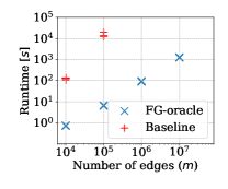
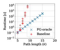
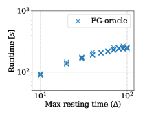
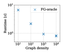
Figure 15. Scalability in synthetic graphs. FG-oracle is fine-grained oracle.

Extracting an optimal solution. Our second set of experiments compares the runtime of the algorithm for extracting an optimal restless path between a source and a destination using the decision oracle and the fine-grained oracle. Recall that the algorithm only returns a yes/no answer for the existence of a solution and we need multiple queries to the oracle to obtain a solution. Using a decision oracle we require $\mathscr{O}(k\log n\log\tau)$ queries in expectation to obtain an optimum solution as compared to $k$ queries using a fine-grained oracle (see Section 5.9). In Figure 16 we compare the runtime (left) and the peak-memory usage (center) of the decision oracle and the fine-grained oracle for extracting an optimum solution for five independent random power-law graphs for each configuration of $n=10^{3},\dots,10^{7}$ with fixed values of $d=100$, $\tau=100$, $\Delta=10$, $\delta:V\rightarrow\{\Delta\}$ and $k=10$. The source and the destination are chosen at random. We observe little variance in runtime for the fine-grained extraction as compared to oracle extraction. For large graphs with hundred million edges the fine-grained extraction is up to four times faster than the oracle extraction. Even though in theory we reduce the number of queries by a factor of $\log n\log\tau$, in practice we do not obtain a significant improvement in the empirical runtime. When extracting a solution using the decision oracle, recall that for each query of the oracle we recursively divide the graph into smaller subgraphs. For each smaller subgraph, we build the multilinear sieve and thereby reduce the empirical runtime of each query. In addition, while the the expected number of queries is bounded by $\mathscr{O}(k\log n\log\tau)$ in worst case, this bound is not always met in practice. For a given instance, the number of queries required to extract a $k$-vertex subgraph varies depending on the source and the destination, resulting in high variance in the extraction time for extraction via self-reducibility. However, there is considerably less variance in the runtime of the fine-grained extraction approach.

The experiments are executed on the computenode configuration using all cores. We report the runtime of extraction for the $k\text{\sc-Restless\-Motif}$ instances, but the runtimes are similar for the $k\text{\sc-Restless\-Path}$ instances.

Graph topology. Here we study the effect of graph topology on runtime of the algorithm. In Figure 16 (right), we report the runtime of the algorithm for five independent $d$-regular random graph instances for each configuration of $n=10^{2},\dots,10^{5}$, $d=100$, $\tau=100$, $\Delta=10$, $\delta:V\rightarrow\{\Delta\}$, and $k=10$. Power-law graphs with $n=10^{2},\dots,10^{6}$ with fixed values of $d=100$, $k=10$, $\tau=100$, $\Delta=10$, $\delta:V\rightarrow\{\Delta\}$, $\alpha=-1.0$, and $w=100$. We observe no significant change in the runtime with the change in the graph topology. The experiments are executed on the workstation using all cores. We report the runtime for the $k\text{\sc-Restless\-Motif\-Reach}$ problem instances, but the runtimes are similar for other problem instances.

Extracting a solution	Memory usage	Graph topology

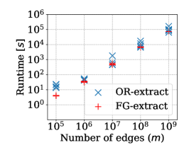
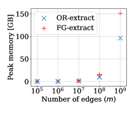
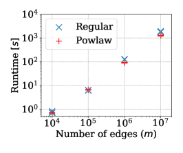
Figure 16. Extracting a solution and topology invariance. OR-extract is solution extraction using decision oracle and FG-extract is solution extraction using fine-grained oracle.

Experiments with real-world graphs. Our next set of experiments reports the runtime of the algorithm for finding restless reachability and extracting a restless path in real-world datasets. The description of the datasets used for our experiments is available in Section 6.2.

In Table 4 and 5 we report the runtime for finding restless reachability in real-worlds graphs with $k=5$ and $k=10$, respectively. For each dataset we report the maximum runtime of five independent runs by choosing the source vertex $s\in V$ uniformly at random for each $k\in\{5,10\}$, for fixed value of the maximum resting time $\Delta=10$, and $\delta:V\rightarrow\{\Delta\}$, i.e., the resting time is constant for all the vertices except the source $s$, which has the maximum resting time $\delta(s)=\tau$. In Column 2 we report the runtime for solving the $k\text{\sc-Restless\-Reach}$ problem, while Column 3 reports the runtime for solving the RestlessReach problem by restricting the path length to $k-1$. Note that here we solve the $\textit{atm-}k\text{\sc-Restless\-Reach}$ problem where we find the set of vertices that are reachable from a given source via a restless path with length at most $k-1$. Column 4 is the ratio of Column 3 and Column 2. Next, in Columns 5 and 6 we report the runtime of extracting a solution using a decision oracle and a fine-grained oracle, respectively. Column 7 is the ratio of Column 6 and Column 5. Finally, in Column 8, we report the peak memory usage of the fine-grained extraction. All runtimes are in seconds. The experiments are executed on computenode configuration using all cores.

We can solve restless reachability in each real-world graph dataset in Table 2 in less than one minute by restricting the length of the restless path $k$ to 5, and in less than two hours using at most 14 Gb of memory for $k=10$. For instance, we can solve restless reachability by limiting $k$ to $10$ in a real-world graph dataset with more than 37 million directed edges and more than 19 thousand timestamps in less than one hour on a Haswell desktop using less than 6 Gb of memory. The reported runtimes are in seconds.

From the results (see Column 3), we see that solving $\textit{atm-}k\text{\sc-Restless\-Reach}$ takes less than twice the empirical running time than that of $k\text{\sc-Restless\-Reach}$, in most of the input graph instance. Extracting a solution using fine-grained extraction is effective for large graphs, given that $k$ is not too large. For instance, we obtain an 8-time speedup in computation using fine-grained extraction as compared to oracle extraction in a graph with more than hundred thousand vertices and more than eight hundred thousand edges with $k=10$.

Table 4. Experiments with real-world datasets ($k=5$). For a description of the columns, see the main text.

	Reachability			Extraction ($k=5$)
	$k=5$	$k\leq 5$	Ratio	Fine-grained	Decision	Speedup	Memory
Dataset	(seconds)	(seconds)		(seconds)	(seconds)		(Gb)
Copenhagen
Calls	1.72	2.66	1.55	1.71	1.80	1.05	0.48
SMS	1.91	2.59	1.36	1.84	1.88	1.02	0.48
Socio-patterns
LH10	8.18	13.06	1.60	8.24	8.27	1.00	3.28
InVS13	25.78	39.93	1.55	25.42	25.45	1.00	6.95
InVS15	39.21	59.38	1.51	42.30	38.36	0.91	13.18
SFHH	6.91	10.36	1.50	7.18	8.45	1.18	1.47
LyonSchool	22.39	32.56	1.45	22.58	27.33	1.21	1.70
Thiers13	51.76	73.39	1.42	51.46	55.27	1.07	5.38
Koblenz
sqwikibooks	1.63	3.60	2.21	1.69	2.14	1.27	0.85
pswiktionary	6.42	10.67	1.66	6.84	7.28	1.06	3.70
sawikisource	9.96	17.21	1.73	13.60	16.63	1.22	6.58
knwiki	21.42	31.50	1.47	23.68	25.22	1.06	12.27
epinions	7.76	12.41	1.60	7.44	24.36	3.27	3.57
Transport
Kuopio	0.49	0.78	1.57	0.51	0.86	1.70	0.10
Rennes	0.76	1.45	1.92	0.74	1.21	1.63	0.25
Grenoble	0.88	1.41	1.60	0.86	1.25	1.45	0.29
Venice	1.03	1.63	1.58	1.33	1.39	1.05	0.39
Belfast	0.82	2.31	2.81	0.89	1.31	1.47	0.31
Canberra	1.08	1.73	1.59	1.07	1.57	1.47	0.43
Turku	0.86	1.51	1.75	0.95	1.31	1.38	0.33
Luxembourg	0.86	1.19	1.38	0.97	1.20	1.24	0.24
Nantes	1.27	1.96	1.54	1.28	1.42	1.11	0.43
Toulouse	1.37	2.32	1.69	1.52	1.94	1.28	0.59
Palermo	1.25	1.86	1.49	1.30	1.57	1.21	0.40
Bordeaux	1.71	2.64	1.54	1.70	1.94	1.14	0.64
Antofagasta	0.70	0.87	1.23	0.68	1.58	2.34	0.11
Detroit	2.63	4.13	1.57	2.50	2.93	1.17	1.22
Winnipeg	2.33	3.33	1.43	2.31	2.69	1.17	0.94
Brisbane	3.92	5.62	1.43	3.77	4.12	1.09	1.76
Adelaide	3.22	4.72	1.47	3.04	3.58	1.18	1.36
Dublin	2.10	3.04	1.45	2.04	2.50	1.23	0.82
Lisbon	3.36	5.27	1.57	3.20	3.69	1.15	1.47
Prague	3.11	4.52	1.45	2.95	3.21	1.09	1.11
Helsinki	3.69	5.06	1.37	3.49	3.97	1.14	1.46
Athens	3.54	6.29	1.78	3.40	3.91	1.15	1.46
Berlin	2.95	3.93	1.33	3.31	3.69	1.11	1.01
Rome	4.59	6.01	1.31	4.44	4.99	1.13	1.70
Melbourne	8.24	12.61	1.53	8.56	8.18	0.96	4.00
Sydney	12.15	17.98	1.48	11.10	11.39	1.03	5.20
Paris	7.98	10.72	1.34	7.54	7.44	0.99	2.33

Table 5. Experiments with real-world datasets ($k=10$). For description of the columns, please see the main text.

	Reachability			Extraction ($k=10$)
	$k=10$	$k\leq 10$	Ratio	Fine-grained	Decision	Speedup	Memory
Dataset	(seconds)	(seconds)		(seconds)	(seconds)		(Gb)
Copenhagen
Calls	88.98	152.91	1.72	90.60	194.03	2.14	0.48
SMS	89.32	153.67	1.72	88.36	195.87	2.22	0.48
Socio-patterns
LH10	411.13	719.49	1.75	417.43	532.08	1.27	3.28
InVS13	1 292.91	2 342.52	1.81	1 309.36	1 613.37	1.23	6.95
InVS15	1 871.23	3 414.07	1.82	1 966.12	2 155.92	1.10	13.18
SFHH	314.48	569.10	1.81	318.29	581.37	1.83	1.47
LyonSchool	1 284.53	2 294.68	1.79	1 298.16	1 849.85	1.42	1.70
Thiers13	2 666.22	4 687.66	1.76	2 663.80	3 233.05	1.21	5.38
Koblenz
sqwikibooks	70.78	131.26	1.85	72.20	257.57	3.57	0.85
pswiktionary	267.32	478.48	1.79	283.14	909.79	3.21	3.71
sawikisource	464.38	856.73	1.84	495.80	1 450.61	2.93	6.59
knwiki	909.25	1 659.58	1.83	969.38	2 995.04	3.09	12.28
epinions	286.11	522.78	1.83	375.55	3 051.37	8.13	3.58
Transport
Kuopio	25.08	43.45	1.73	25.42	116.30	4.58	0.10
Rennes	32.15	59.12	1.84	34.24	161.09	4.71	0.25
Grenoble	38.38	68.99	1.80	39.15	155.41	3.97	0.29
Venice	50.07	84.05	1.68	49.62	176.52	3.56	0.39
Belfast	36.29	69.19	1.91	39.32	172.56	4.39	0.31
Canberra	48.00	86.93	1.81	48.93	182.02	3.72	0.43
Turku	39.46	75.04	1.90	43.81	158.19	3.61	0.33
Luxembourg	37.15	65.73	1.77	39.68	140.88	3.55	0.24
Nantes	51.82	87.37	1.69	52.35	150.44	2.87	0.43
Toulouse	62.96	113.45	1.80	62.54	203.01	3.25	0.59
Palermo	47.20	93.09	1.97	52.74	198.76	3.77	0.40
Bordeaux	67.52	124.61	1.85	69.16	208.33	3.01	0.64
Antofagasta	23.72	41.53	1.75	25.26	112.66	4.46	0.11
Detroit	111.74	201.14	1.80	107.84	288.48	2.68	1.22
Winnipeg	88.13	162.17	1.84	93.29	231.43	2.48	0.94
Brisbane	147.66	268.12	1.82	153.42	320.82	2.09	1.76
Adelaide	122.11	221.79	1.82	124.29	312.47	2.51	1.37
Dublin	78.42	142.13	1.81	82.51	205.09	2.49	0.82
Lisbon	134.25	246.37	1.84	137.01	332.89	2.43	1.47
Prague	108.59	199.35	1.84	107.47	245.90	2.29	1.11
Helsinki	130.68	231.65	1.77	136.54	319.97	2.34	1.46
Athens	129.10	233.02	1.80	130.00	324.98	2.50	1.46
Berlin	102.28	179.79	1.76	105.72	233.19	2.21	1.01
Rome	159.08	287.87	1.81	164.57	368.35	2.24	1.70
Melbourne	323.32	590.11	1.83	337.50	631.20	1.87	4.00
Sydney	411.24	732.24	1.78	427.51	866.15	2.03	5.20
Paris	223.02	403.70	1.81	224.21	477.10	2.13	2.33

Reachability. Our next set of experiments studies the restless reachability in socio-patterns dataset. In particular we solve the $\textit{atm-}k\text{\sc-Restless\-Reach}$ problem where we find the set of vertices reachable from a given source via a restless path of length at most $k-1$. Reachability is the ratio of the number of vertices that are reachable with a restless path to the total number of vertices. In Figure 17 we report the variance and mean of reachability as a time-series for five independent graph instances for each dataset with $\Delta=5$ (top-row) and $\Delta=20$ (bottom-row). More precisely, for a given dataset we generate five graph instances by choosing a source vertex uniformly at random and assign the resting times uniformly at random in the range $[\Delta]$. We limit the length of the restless path to $9$, i.e., $k=10$ and solve the $\textit{atm-}k\text{\sc-Restless\-Reach}$ problem.

We observe high variance in reachability among the independent source vertices for LH10, InVS15, LyonSchool, and Thiers13 datasets, and smaller variance for InVS13 and SFHH. We also see that in all datasets, except LH10, reachability approaches its maximum value 1, within the total number of timestamps available in each dataset, however, this happens at different times for each dataset, and with a different pace.

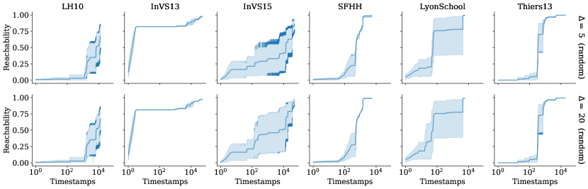
Figure 17. Restless reachability in real-world datasets with $\Delta=5$ (top-row) and $\Delta=20$ (bottom-row) with $\delta:V\rightarrow[\Delta]$ assigned uniformly at random, and $k=10$ (fixed).

In Table 6, we report the runtime for solving the $\textit{atm-}k\text{\sc-Restless\-Reach}$ problem in socio-patterns datasets. The reported runtime is the maximum of five independent runs by choosing the source vertex $s\in V$ uniformly at random with $k=10$ (fixed) and $\Delta=5,10$, $\delta:V\rightarrow\{\Delta\}$ (fixed). The resting time is constant for all the vertices except the source $s$, which has the maximum resting time $\delta(s)=\tau$. For instance, we can solve $k\text{\sc-Restless\-Reach}$ problem by limiting $k=10$ in a real-world graph dataset with more than 37 million directed edges and more than 19 thousand timestamps in less than one hour on workstation configuration using less than 6 Gb of memory. The reported runtimes are in seconds.

Table 6. Computing restless reachability in socio-patterns dataset using the workstation configuration. We report runtime for solving $\textit{atm-}k\text{\sc-Restless\-Reach}$ problem with $k=10$ (fixed).

Dataset	$n$	$m$	$\tau$	$\Delta=5$	$\Delta=10$
				(seconds)	(seconds)
LH10	73	300 252	12 960	156.8 s	158.7
InVS13	95	788 494	49 679	357.1 s	386.5
InVS15	219	2 566 388	49 679	657.2 s	733.2
SFHH	403	2 834 970	5 328	245.0 s	346.3
LyonSchool	242	13 188 984	5 887	853.6 s	1 341.2
Thiers13	328	37 226 078	19 022	2 083.1 s	3 399.5

6.5. Case study: comparing immunization strategies

Our final set of experiments studies the change in restless reachability in the presence of a set of barrier vertices $S^{\prime}\subseteq V$ called separators, which must not be included in the restless path. In an epidemic model, the separators can be viewed as a subset of the population, all immune and/or vaccinated. It is known that finding a set of temporal separators with minimum size, which destroy all the restless paths between any two vertices, is $\sum_{2}^{P}$-hard (Casteigts et al., 2020). A promising heuristic to finding a minimum set of separators is choosing the vertices with high temporal-betweenness centrality. Unfortunately, computing the betweenness centrality in temporal graphs is intractable (Buß et al., 2020).

The experiments performed in this case study are to evaluate the effectiveness of our algorithm to answer queries for finding an effective immunization strategy in an epidemic model where the disease propagation is via a restless path. To demonstrate this we use two heuristics for finding separators: ($i$) choose vertices at random and ($ii$) choose vertices with maximum temporal degree. Note that these immunization strategies are simple and without theoretical guarantees. Towards this end, we would like to investigate effective approximation or heuristic schemes to find temporal separators, which reduce the fraction of vertices reachable from a given source vertex via a restless path in future work.

Given an instance $(G=(V,E),s,k)$ of the $k\text{\sc-Restless\-Reach}$ problem and a set $S^{\prime}\subseteq V$ of separators, we introduce a coloring function $c:V\setminus\{S^{\prime}\cup s\}\rightarrow\{1\}$, $c(s)=2$ and $c:S^{\prime}\rightarrow\{3\}$ and $M=\{1^{\ell-1},2\}$ for $\ell\in[k]$. We query the FineGrainedOracle with instance $(G^{\prime}=(V,E\setminus\{u,s,i\}\in E),c,\ell,M)$ for each $\ell\in\{2,\dots,k\}$. By assigning color $3\notin M$ to the separators in $S^{\prime}$, we make sure that none of the separators are part of the restless path agreeing the multiset of colors in $M$. Note that here we solve the $\textit{atm-}k\text{\sc-Restless\-Reach}$ problem, in other words we find the set of vertices which are reachable from the source via a restless path of length at most $k-1$.

In Figure 18, we report the variance of reachability in real-world graphs by choosing $5\%$ of the vertices uniformly a random (top-row) and $5\%$ of the vertices with maximum degree (second-row) as separators. Figure 19 reports the same experiments with $5\%$ replaced with $25\%$. For each dataset we generate five graph instances, choose source vertices at random and assign resting times uniformly at random in the range $[\Delta]$ for $\Delta=10$. Note that we use the same instances in the reachability experiments described above. Reachability is the ratio of number of reachable vertices to the total number of vertices excluding separators. From the experimental results we observe high variance in the reachability among independent source vertices and the rate of increase of the reachability with time varies depending on the source vertex. More importantly, even though we expect (empirically) that by choosing vertices with high degree as separators should decrease the reachability as compared to choosing the vertices at random, this is not true for all the datasets. We only observe this phenomenon in SFHH and Thiers13 datasets for choosing $5$% of the vertices as separators and in InVS15 and LyonSchool datasets while choosing $25$% of the vertices as separators.

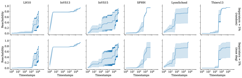
Figure 18. Restless reachability in real-world datasets in the presence of $5\%$ separators. $\Delta=10$, $\delta:V\rightarrow[\Delta]$ assigned uniformly at random and $k=10$ (fixed).

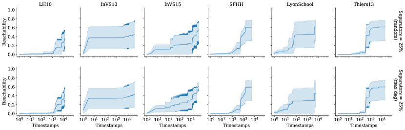
Figure 19. Restless reachability in real-world datasets in the presence of $25\%$ separators. $k=10$, $\Delta=10$, $\delta:V\rightarrow[\Delta]$ assigned uniformly at random.

In Figure 20, we report the variance of reachability in real-world graphs by choosing $5\%$, $10\%$, and $25\%$ of the vertices uniformly a random (top-row) and $5\%$, $10\%$, and $25\%$ of the vertices with maximum degree (second-row) as separators. Again, for each dataset we generate five graph instances, choose source vertices at random and assign resting time uniformly at random in the range $[\Delta]$ for $\Delta=10$. Note that we use the same instances in the reachability experiments described above. We observe that reachability reduces with an increase in the number of separators, as expected. Again, even though it is expected (empirically) that choosing vertices with maximum degree to reduce the reachability significantly compared to choosing separators at random, surprisingly enough, this is not true for all datasets. For instance in LyonSchool dataset choosing 10% of the separators at random reduces the average reachability more than choosing vertices with maximum degree as separators. So the heuristic approach of choosing vertices with maximum degrees might not be effective across datasets. This presents us a interesting question of finding a small a set of separators in temporal graphs under resting time restrictions. Also note that the input graph datasets are small world graphs, meaning that the diameter of the underlying graph is small, so the vertices are highly connected (see Table 2).

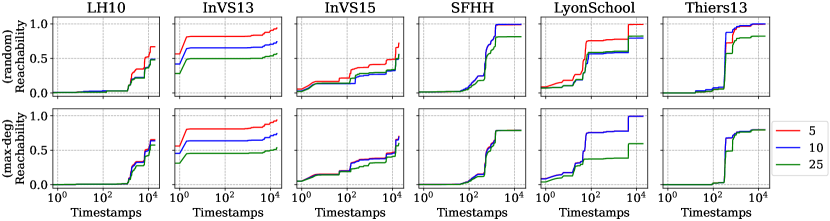
Figure 20. Restless reachability in real-world datasets in the presence of separators. $k=10$ (fixed), $\Delta=10$, $\delta:V\rightarrow[\Delta]$ assigned uniformly at random.

7. Conclusions and future work

In this work, we studied a family of reachability problems in temporal and vertex-colored temporal graphs under waiting-time restrictions. We presented an algebraic algorithm framework for solving restless reachability problem we proposed, running in $\mathscr{O}(2^{k}km\Delta)$ time and $\mathscr{O}(n\tau)$ space. We presented evidence that the algorithms for solving variants of the restless reachability problems involving colors presented in this work are optimal under plausible complexity-theoretic assumptions. Further, we engineered an open-source implementation of our algorithm, and demonstrated its viability in experiments on graphs with millions of temporal edges from real-world datasets. Finally, we applied the algorithm we developed in a case study for estimating the change in disease spreading with the presence of people with immunity. Our finding is that heuristic approaches such as selecting vertices with high degree as separators are not effective in all the graph datasets. Towards this end, we would like to investigate effective ways to choose a small set of separators under waiting time restrictions to contain the spread of the disease in the network.

We believe our algorithms, based on multilinear and constrained multilinear sieving, can be extended even further to solve a range of other pattern-detection problems in temporal graphs, including finding arborescences, connected temporal subgraphs and temporal subgraphs with additional color constraints on the vertices. We also note that our temporal reachability setting corresponds to the SIS (susceptible-infectious-susceptible) epidemic model. Another interesting direction is to develop algorithms for temporal reachability that corresponds to the SIR (susceptible-infectious-removed) model.

Table 7. List of symbols.

Symbol	Description
Graphs
$G=(V,E)$	graph $G$ with vertex set $V$ and edge set $E$
$n$	number of vertices
$m$	number of edges
$m_{i}$	number of edges at time stamp $i$
$\Delta$	maximum resting time
$\tau$	maximum timestamp
$k$	length of path or walk
$\delta:V\rightarrow[\Delta]$	restless function mapping vertices to resting time
$N_{i}(u)$	in-neighbors of vertex $u$ at time stamp $i$
$G^{\downarrow}$	underlying static graph of temporal graph $G$
${G^{\uparrow}(\delta)}$	$\delta$-expansion of temporal graph $G$
Coloring
$C$	set of colors
$c:V\rightarrow C$	coloring function mapping vertices to colors
$M$	multiset of colors
$\mu(s)$	number of occurrences of color $s$ in $M$
Polynomials
$\mathscr{P}$	polynomial encoding of temporal walks
$\chi$	polynomial encoding of restless walks
$\zeta$	evaluation polynomial of restless walks
$x_{u}$	$x$-variable encoding vertex $u$
$y_{uv,\ell,j}$	$y$-variable encoding edge $(u,v,j)$ at position $\ell$
$\vec{x}$	vector of $x$ variables
$\vec{y}$	vector of $y$ variables
$\vec{z}$	vector of $z$ variables

Conflict of interest

The authors declare that they have no conflict of interest.

References

- (1)
- Agrawal et al. (1989) Rakesh Agrawal, Alexander Borgida, and Hosagrahar Visvesvaraya Jagadish. 1989. Efficient management of transitive relationships in large data and knowledge bases. SIGMOD Record 18, 2 (1989), 253–262.
- Alon et al. (2008) Noga Alon, Phuong Dao, Iman Hajirasouliha, Fereydoun Hormozdiari, and S. Cenk Sahinalp. 2008. Biomolecular network motif counting and discovery by color coding. Bioinformatics 24, 13 (07 2008), 241–249.
- Anand and Chatterjee (2017) Rajat Anand and Samrat Chatterjee. 2017. Tracking disease progression by searching paths in a temporal network of biological processes. PLOS one 12, 4 (2017), e0176172.
- Badie-Modiri et al. (2020) Arash Badie-Modiri, Márton Karsai, and Mikko Kivelä. 2020. Efficient limited-time reachability estimation in temporal networks. Physical Review E 101, 5 (2020), 052303.
- Bakshy et al. (2012) Eytan Bakshy, Itamar Rosenn, Cameron Marlow, and Lada Adamic. 2012. The role of social networks in information diffusion. In WWW. ACM, 519–528.
- Benson et al. (2015) Erik Benson, Abdulmelik Mohammed, Johan Gardell, Sergej Masich, Eugen Czeizler, Pekka Orponen, and Björn Högberg. 2015. DNA rendering of polyhedral meshes at the nanoscale. Nature 523, 7561 (2015), 441–444.
- Björklund et al. (2017) Andreas Björklund, Thore Husfeldt, Petteri Kaski, and Mikko Koivisto. 2017. Narrow sieves for parameterized paths and packings. JCSS 87 (2017), 119–139.
- Björklund et al. (2013) Andreas Björklund, Petteri Kaski, and Łukasz Kowalik. 2013. Probably optimal graph motifs. In STACS. Schloss Dagstuhl-Leibniz-Zentrum fuer Informatik, 20–31.
- Björklund et al. (2014a) Andreas Björklund, Petteri Kaski, and Łukasz Kowalik. 2014a. Determinant Sums for Undirected Hamiltonicity. SIAM J. Comput. 43, 1 (2014), 280–299.
- Björklund et al. (2014b) Andreas Björklund, Petteri Kaski, and Łukasz Kowalik. 2014b. Fast Witness Extraction Using a Decision Oracle. In ESA. Springer, 149–160.
- Björklund et al. (2016) Andreas Björklund, Petteri Kaski, and Łukasz Kowalik. 2016. Constrained Multilinear Detection and Generalized Graph Motifs. Algorithmica 74, 2 (2016), 947–967.
- Björklund et al. (2015) Andreas Björklund, Petteri Kaski, Łukasz Kowalik, and Juho Lauri. 2015. Engineering Motif Search for Large Graphs. In ALENEX. SIAM, 104–118.
- Bollobás (2001) Béla Bollobás. 2001. Random Graphs (second ed.). Cambridge UP.
- Bonchi et al. (2014) Francesco Bonchi, Aristides Gionis, Francesco Gullo, and Antti Ukkonen. 2014. Distance oracles in edge-labeled graphs.. In EDBT. DBLP, 547–558.
- Bullmore and Sporns (2009) Ed Bullmore and Olaf Sporns. 2009. Complex brain networks: graph theoretical analysis of structural and functional systems. Nature Reviews Neuroscience 10, 3 (2009), 186–198.
- Buß et al. (2020) Sebastian Buß, Hendrik Molter, Rolf Niedermeier, and Maciej Rymar. 2020. Algorithmic Aspects of Temporal Betweenness. In KDD. ACM, 2084–2092.
- Casteigts et al. (2020) Arnaud Casteigts, Anne-Sophie Himmel, Hendrik Molter, and Philipp Zschoche. 2020. Finding Temporal Paths Under Waiting Time Constraints. In ISAAC. Schloss Dagstuhl-Leibniz-Zentrum für Informatik, 30:1–30:18.
- Chen and Chen (2008) Yangjun Chen and Yibin Chen. 2008. An efficient algorithm for answering graph reachability queries. In ICDE. IEEE, 893–902.
- Cheng et al. (2020) Chun-Hung Cheng, Yong-Hong Kuo, and Ziye Zhou. 2020. Outbreak minimization vs influence maximization: an optimization framework. BMC Medical Informatics and Decision Making 20, 1 (2020), 1–13.
- Cohen et al. (2003) Edith Cohen, Eran Halperin, Haim Kaplan, and Uri Zwick. 2003. Reachability and distance queries via 2-hop labels. SIAM J. Comput. 32, 5 (2003), 1338–1355.
- Cooke and Halsey (1966) Kenneth L Cooke and Eric Halsey. 1966. The shortest route through a network with time-dependent internodal transit times. J. Math. Anal. Appl. 14, 3 (1966), 493 – 498.
- Crescenzi et al. (2013) Pilu Crescenzi, Roberto Grossi, Michel Habib, Leonardo Lanzi, and Andrea Marino. 2013. On computing the diameter of real-world undirected graphs. TCS 514 (2013), 84 – 95.
- Cygan et al. (2016) Marek Cygan, Holger Dell, Daniel Lokshtanov, Dániel Marx, Jesper Nederlof, Yoshio Okamoto, Ramamohan Paturi, Saket Saurabh, and Magnus Wahlström. 2016. On problems as hard as CNF-SAT. ACM Trans. on Algorithms 12, 3 (2016), 1–24.
- Cygan et al. (2015) Marek Cygan, Fedor V Fomin, Łukasz Kowalik, Daniel Lokshtanov, Dániel Marx, Marcin Pilipczuk, Michał Pilipczuk, and Saket Saurabh. 2015. Parameterized algorithms. Vol. 4. Springer.
- de Pasquale et al. (2010) Francesco de Pasquale, Stefania Della Penna, Abraham Z. Snyder, Christopher Lewis, Dante Mantini, Laura Marzetti, Paolo Belardinelli, Luca Ciancetta, Vittorio Pizzella, Gian Luca Romani, and Maurizio Corbetta. 2010. Temporal dynamics of spontaneous MEG activity in brain networks. Proc. of the National Academy of Sciences 107, 13 (2010), 6040–6045.
- Dean (2004) Brian C Dean. 2004. Algorithms for minimum-cost paths in time-dependent networks with waiting policies. Networks 44, 1 (2004), 41–46.
- Eubank et al. (2004) Stephen Eubank, Hasan Guclu, VS Anil Kumar, Madhav V Marathe, Aravind Srinivasan, Zoltan Toroczkai, and Nan Wang. 2004. Modelling disease outbreaks in realistic urban social networks. Nature 429, 6988 (2004), 180–184.
- Ferretti et al. (2020) Luca Ferretti, Chris Wymant, Michelle Kendall, Lele Zhao, Anel Nurtay, Lucie Abeler-Dörner, Michael Parker, David Bonsall, and Christophe Fraser. 2020. Quantifying SARS-CoV-2 transmission suggests epidemic control with digital contact tracing. Science 368, 6491 (March 2020), eabb6936.
- Festa (2015) P Festa. 2015. Constrained shortest path problems: state-of-the-art and recent advances. In 2015 17th International Conference on Transparent Optical Networks (ICTON). IEEE, 1–17.
- Fluschnik et al. (2020) Till Fluschnik, Hendrik Molter, Rolf Niedermeier, Malte Renken, and Philipp Zschoche. 2020. Temporal graph classes: A view through temporal separators. TCS 806 (2020), 197 – 218.
- Génois and Barrat (2018) Mathieu Génois and Alain Barrat. 2018. Can co-location be used as a proxy for face-to-face contacts? EPJ Data Science 7, 1 (2018), 11.
- George et al. (2007) Betsy George, Sangho Kim, and Shashi Shekhar. 2007. Spatio-temporal network databases and routing algorithms: A summary of results. In SSTD. Springer, 460–477.
- Glerean et al. (2016) Enrico Glerean, Raj K Pan, Juha Salmi, Rainer Kujala, Juha M Lahnakoski, Ulrika Roine, Lauri Nummenmaa, Sami Leppämäki, Taina Nieminen-von Wendt, Pekka Tani, Jari Saramaki, Mikko Sams, and Iiro Jääskeläinen. 2016. Reorganization of functionally connected brain subnetworks in high-functioning autism. Human Brain Mapping 37, 3 (2016), 1066–1079.
- Gupta et al. (2011) Manish Gupta, Charu C. Aggarwal, and Jiawei Han. 2011. Finding Top-k Shortest Path Distance Changes in an Evolutionary Network. In SSTD. Springer, 130–148.
- Himmel et al. (2019) Anne-Sophie Himmel, Matthias Bentert, André Nichterlein, and Rolf Niedermeier. 2019. Efficient computation of optimal temporal walks under waiting-time constraints. In Complex Networks. Springer, 494–506.
- Holme (2005) Petter Holme. 2005. Network reachability of real-world contact sequences. Physical Review E 71, 4 (2005), 046119.
- Holme and Saramäki (2012) Petter Holme and Jari Saramäki. 2012. Temporal networks. Physics Reports 519, 3 (2012), 97–125.
- Irnich and Desaulniers (2005) Stefan Irnich and Guy Desaulniers. 2005. Shortest path problems with resource constraints. In Column generation. Springer, 33–65.
- Iwata et al. (2016) Yoichi Iwata, Magnus Wahlstrom, and Yuichi Yoshida. 2016. Half-integrality, LP-branching, and FPT algorithms. SIAM J. Comput. 45, 4 (2016), 1377–1411.
- Iwata et al. (2018) Yoichi Iwata, Magnus Wahlstrom, and Yuichi Yoshida. 2018. https://github.com/wata-orz/fvs.
- Jackson and Yariv (2005) Matthew O Jackson and Leeat Yariv. 2005. Diffusion on social networks. In Economie Publique. Citeseer.
- Jin et al. (2010) Ruoming Jin, Hui Hong, Haixun Wang, Ning Ruan, and Yang Xiang. 2010. Computing Label-Constraint Reachability in Graph Databases. In SIGMOD. ACM, New York, NY, USA, 123–134.
- Jin et al. (2009) Ruoming Jin, Yang Xiang, Ning Ruan, and David Fuhry. 2009. 3-hop: a high-compression indexing scheme for reachability query. In ICDM. ACM, 813–826.
- Karp (1972) Richard M Karp. 1972. Reducibility among combinatorial problems. In Complexity of computer computations. Springer, 85–103.
- Kaski et al. (2018) Petteri Kaski, Juho Lauri, and Suhas Thejaswi. 2018. Engineering Motif Search for Large Motifs. In SEA. Schloss Dagstuhl–Leibniz-Zentrum fuer Informatik, 28:1–28:19.
- Kempe et al. (2003) David Kempe, Jon Kleinberg, and Éva Tardos. 2003. Maximizing the spread of influence through a social network. In KDD. ACM, 137–146.
- Koutis (2008) Ioannis Koutis. 2008. Faster Algebraic Algorithms for Path and Packing Problems. In ICALP (LNCS). Springer, 575–586.
- Koutis and Williams (2009) Ioannis Koutis and Ryan Williams. 2009. Limits and Applications of Group Algebras for Parameterized Problems. In ICALP (LNCS). Springer, 653–664.
- Kowalik and Lauri (2016) Łukasz Kowalik and Juho Lauri. 2016. On finding rainbow and colorful paths. TCS 628 (2016), 110 – 114.
- Krauthgamer and Trabelsi (2019) Robert Krauthgamer and Ohad Trabelsi. 2019. The Set Cover Conjecture and Subgraph Isomorphism with a Tree Pattern. In STACS. Schloss Dagstuhl-Leibniz-Zentrum fuer Informatik, 45:1–45:15.
- Kujala (2018) Rainer Kujala. 2018. From the brain to public transport: Applications of network science. Ph.D. Dissertation.
- Kujala et al. (2018) Rainer Kujala, Christoffer Weckström, Richard K Darst, Miloš N Mladenović, and Jari Saramäki. 2018. A collection of public transport network data sets for 25 cities. Scientific Data 5 (2018), 180089.
- Kunegis (2013) Jérôme Kunegis. 2013. KONECT: the Koblenz network collection. In WWW. ACM, 1343–1350. http://konect.uni-koblenz.de/networks/.
- Lin et al. (2016) Sian-Jheng Lin, Tareq Y. Al-Naffouri, Yunghsiang S. Han, and Wei-Ho Chung. 2016. Novel polynomial basis with fast Fourier transform and its application to Reed-Solomon erasure codes. ITIT 62, 11 (2016).
- Mertzios et al. (2019) George B Mertzios, Othon Michail, and Paul G Spirakis. 2019. Temporal network optimization subject to connectivity constraints. Algorithmica 81, 4 (2019), 1416–1449.
- Michail (2016) Othon Michail. 2016. An introduction to temporal graphs: An algorithmic perspective. Internet Mathematics 12, 4 (2016), 239–280.
- Nightingale et al. (2011) Edmund B. Nightingale, John R. Douceur, and Vince Orgovan. 2011. Cycles, Cells and Platters: An Empirical Analysis of Hardware Failures on a Million Consumer PCs. In Proc. of Computer Systems (EuroSys ’11). ACM, 343–356.
- Pastor-Satorras et al. (2015) Romualdo Pastor-Satorras, Claudio Castellano, Piet Van Mieghem, and Alessandro Vespignani. 2015. Epidemic processes in complex networks. Reviews of Modern Physics 87, 3 (2015), 925.
- Peng et al. (2021) You Peng, Xuemin Lin, Ying Zhang, Wenjie Zhang, and Lu Qin. 2021. Answering reachability and K-reach queries on large graphs with label constraints. VLDB (2021), 1–27.
- Peng et al. (2020) You Peng, Ying Zhang, Xuemin Lin, Lu Qin, and Wenjie Zhang. 2020. Answering Billion-Scale Label-Constrained Reachability Queries within Microsecond. VLDB 13, 6 (feb 2020), 812–825.
- Perozzi et al. (2014) Bryan Perozzi, Leman Akoglu, Patricia Iglesias Sánchez, and Emmanuel Müller. 2014. Focused clustering and outlier detection in large attributed graphs. In KDD. 1346–1355.
- Prakash et al. (2013) B Aditya Prakash, Lada Adamic, Theodore Iwashyna, Hanghang Tong, and Christos Faloutsos. 2013. Fractional immunization in networks. In SDM. SIAM, 659–667.
- Prakash et al. (2010) B Aditya Prakash, Hanghang Tong, Nicholas Valler, Michalis Faloutsos, and Christos Faloutsos. 2010. Virus propagation on time-varying networks: Theory and immunization algorithms. In ECML-PKDD. Springer, 99–114.
- Rozenshtein et al. (2016) Polina Rozenshtein, Aristides Gionis, B Aditya Prakash, and Jilles Vreeken. 2016. Reconstructing an epidemic over time. In KDD. ACM, 1835–1844.
- Sapiezynski et al. (2019) Piotr Sapiezynski, Arkadiusz Stopczynski, David Dreyer Lassen, and Sune Lehmann. 2019. Interaction data from the copenhagen networks study. Scientific Data 6, 1 (2019), 1–10.
- Schwartz (1980) Jacob T. Schwartz. 1980. Fast Probabilistic Algorithms for Verification of Polynomial Identities. JACM 27, 4 (1980), 701–717.
- Schwikowski et al. (2000) Benno Schwikowski, Peter Uetz, and Stanley Fields. 2000. A network of protein–protein interactions in yeast. Nature Biotechnology 18, 12 (2000), 1257–1261.
- Sengupta et al. (2019) Neha Sengupta, Amitabha Bagchi, Maya Ramanath, and Srikanta Bedathur. 2019. Arrow: Approximating reachability using random walks over web-scale graphs. In ICDE. IEEE, 470–481.
- Simon (1988) Klaus Simon. 1988. An improved algorithm for transitive closure on acyclic digraphs. TCS 58, 1-3 (1988), 325–346.
- Thejaswi (2020) Suhas Thejaswi. 2020. Restless-reachability-experimental-v1.0: release. https://github.com/suhastheju/restless-reachability
- Thejaswi and Gionis (2020) Suhas Thejaswi and Aristides Gionis. 2020. Pattern detection in large temporal graphs using algebraic fingerprints. In SDM. SIAM, 37–45.
- Thejaswi et al. (2020) Suhas Thejaswi, Aristides Gionis, and Juho Lauri. 2020. Finding Path Motifs in Large Temporal Graphs Using Algebraic Fingerprints. Big Data (2020), 335–362.
- Thompson et al. (2017) William Hedley Thompson, Per Brantefors, and Peter Fransson. 2017. From static to temporal network theory: Applications to functional brain connectivity. Network Neuroscience 1, 2 (2017), 69–99.
- Thorup and Zwick (2005) Mikkel Thorup and Uri Zwick. 2005. Approximate distance oracles. J. ACM 52, 1 (2005), 1–24.
- Tong et al. (2007) Hanghang Tong, Christos Faloutsos, Brian Gallagher, and Tina Eliassi-Rad. 2007. Fast best-effort pattern matching in large attributed graphs. In KDD. ACM, 737–746.
- Tong et al. (2010) Hanghang Tong, B Aditya Prakash, Charalampos Tsourakakis, Tina Eliassi-Rad, Christos Faloutsos, and Duen Horng Chau. 2010. On the vulnerability of large graphs. In ICDM. IEEE, 1091–1096.
- Von Ferber et al. (2009) Christian Von Ferber, Taras Holovatch, Yu Holovatch, and V Palchykov. 2009. Public transport networks: empirical analysis and modeling. The European Physical Journal B 68, 2 (2009), 261–275.
- Wang et al. (2021) Yishu Wang, Ye Yuan, Hao Wang, Xiangmin Zhou, Congcong Mu, and Guoren Wang. 2021. Constrained Route Planning over Large Multi-Modal Time-Dependent Networks. In ICDE. IEEE, 313–324.
- Williams (2009) Ryan Williams. 2009. Finding paths of length in time. IPL 109, 6 (2009), 315–318.
- Wu et al. (2014) Huanhuan Wu, James Cheng, Silu Huang, Yiping Ke, Yi Lu, and Yanyan Xu. 2014. Path Problems in Temporal Graphs. Proc. VLDB Endow. 7, 9 (2014), 721–732.
- Wu et al. (2016a) H. Wu, J. Cheng, Y. Ke, S. Huang, Y. Huang, and H. Wu. 2016a. Efficient Algorithms for Temporal Path Computation. TKDE 28, 11 (2016), 2927–2942.
- Wu et al. (2016b) H. Wu, Y. Huang, J. Cheng, J. Li, and Y. Ke. 2016b. Reachability and time-based path queries in temporal graphs. In ICDE. 145–156.
- Xuan et al. (2003) B Bui Xuan, Afonso Ferreira, and Aubin Jarry. 2003. Computing shortest, fastest, and foremost journeys in dynamic networks. Journal of FOCS 14, 02 (2003), 267–285.
- Yu and Cheng (2010) Jeffrey Xu Yu and Jiefeng Cheng. 2010. Graph reachability queries: A survey. In Managing and Mining Graph Data. Springer, 181–215.
- Yuan et al. (2019) Ye Yuan, Xiang Lian, Guoren Wang, Yuliang Ma, and Yishu Wang. 2019. Constrained shortest path query in a large time-dependent graph. VLDB 12, 10 (2019), 1058–1070.
- Zhang et al. (2016) Zi-Ke Zhang, Chuang Liu, Xiu-Xiu Zhan, Xin Lu, Chu-Xu Zhang, and Yi-Cheng Zhang. 2016. Dynamics of information diffusion and its applications on complex networks. Physics Reports 651 (2016), 1–34.
- Zippel (1979) Richard Zippel. 1979. Probabilistic algorithms for sparse polynomials. In ISSAC (LNCS, Vol. 72). Springer, 216–226.
- Zschoche et al. (2020) Philipp Zschoche, Till Fluschnik, Hendrik Molter, and Rolf Niedermeier. 2020. The complexity of finding small separators in temporal graphs. JCSS 107 (2020), 72 – 92.