Difference-in-Differences: Bridging Normalization and Disentanglement in PG-GAN
Abstract
What mechanisms causes GAN’s entanglement? Although developing disentangled GAN has attracted sufficient attention, it is unclear how entanglement is originated by GAN transformation. We in this research propose a difference-in-difference (DID) counterfactual framework to design experiments for analyzing the entanglement mechanism in on of the Progressive-growing GAN (PG-GAN). Our experiment clarify the mechanisms how pixel normalization causes PG-GAN entanglement during a input-unit-ablation transformation. We discover that pixel normalization causes object entanglement by in-painting the area occupied by ablated objects. We also discover the unit-object relation determines whether and how pixel normalization causes objects entanglement. Our DID framework theoretically guarantees that the mechanisms that we discover is solid, explainable and comprehensively.
1 Introduction
Understanding the entanglement stands on the stage center of the deep learning research because entanglement is deeply rooted in the complex computational process of neural network models (Karpathy et al., 2015; Kulkarni et al., 2015; Higgins et al., 2016) while indicating non-predicable biases. Therefore, developing an output-disentangle neural network model has attracted a significant amount of attention from deep-learning society. However, the absence of analytical understanding about the mechanism causing output entanglement prevents us from discussing whether and when a neural network’s architecture can systematically avoid relative biases.
On the other hand, it is a challenge to examine the mechanism causing GAN (Goodfellow et al., 2014; Radford et al., 2015; Zhang et al., 2019; Chen et al., 2016) entanglement. GAN’s deep neural network structure obstructs the progress of theoretical analyses, while the experimental approach proposed by the most recent studies (Zhou et al., 2018; Selvaraju et al., 2017; Simonyan et al., 2013; Olah et al., 2018; Schwab & Karlen, 2019) is incapable of enlightening GAN’s inside structure. Current experimental approaches in the literature are designed for generating counterfactual scenarios (Imbens & Rubin, 2015; Pearl, 2009) with and without the input changes (Bau et al., 2017; represent). In contrast, understanding GAN’s internal mechanism causing entanglement asks for an experimental design that can generate counterfactual scenarios with and without GAN’s functioning. Thus, a new experimental design is necessary for studying the mechanism of GAN entanglement.
We in this research develop a difference-in-difference (DID) (Ciani & Fisher, 2018; Goodman-Bacon, 2018; Abadie, 2005; Athey & Imbens, 2006) experiment to analyze the entanglement mechanism originated in the pixel-normalization operation of the Progressive-growing generative adversarial network (PG-GAN) (Karras et al., 2017). We select to research PG-GAN because of two reasons. First, PG-GAN is an approach of generating a high-resolution figure including various objects that can entangle with each other. Second, the recent progress in literature has well prepared for applying DID to study PG-GAN’s entanglement. (Besserve et al. (2018a)) rigorously defined the concept of operation-based object disentanglement in a figure generated by GAN. (Bau et al. (2018)) has developed an approach to clarify the causal ties between input units and output objects. Based on these two studies, we design a DID experiment to examine how pixel normalization causes object entanglement during a unit-ablating transformation.
Our results conclude that pixel normalization causes entanglement by in-painting the area belonging to ablated objects. Once the in-painted objects are different from those surrounding the in-painted area, an entanglement effect occurs. Entanglement caused by pixel normalization can be further clustered according to the types of in-painted objects. If the in-painted objects are from the same types as the ablated one, the entanglement effect deactivates the ablating transformation. We refer to this type of entanglement as the “deactivating-ablation entanglement” or Type-1 entanglement. Otherwise, the entanglement effect causes unwanted objects’ appearance associated with ablating, referred to as the “mis-ablation entanglement” or Type-2 entanglement by this research. The difference-in-difference experiment also clarifies that the characteristics of unit-object causal relation determine the types of in-painted objects.
We summarize our three contributions in this research:
-
•
We explain the internal mechanism of how pixel normalization causes object entanglement under ablating transformation. Because of our insights into the black-box of PG-GAN, we also clarify the necessary conditions when objects are disentangled.
-
•
We clarify the mechanism how unit-object causal relation determine whether and how disentanglement occurs.
-
•
We propose an experimental approach to analyze PG-GAN’s functioning mechanism based on the DID counterfactual framework, which can be generalized for broader deep neural network studies. Designing appropriate DID experiments to examine the functioning mechanism of neural network deserves further discussion.
Our understanding about entanglement provide a new perspective on entanglement research, which can enable of a sequence further research. For instance, it is possible to design an ablation method rather than modifying PG-GAN to avoid entanglement according to the understanding about how pixel normalization causes entanglement over objects. The understanding the deactivating-ablation entanglement also allows us to examine the robustness of objects in a figure once some input units are unexpected losses.
2 Preliminary: PG-GAN and Disentanglement
In this work, we are studying what the disentanglement properties are in the ablation transformation of PG-GAN (Karras et al. (2017)). PG-GAN is good at producing versatile objects with details while preserving the model efficiency. It adopts a progressive layer-growing strategy for fine-grained details and pixel normalization for training robustness.
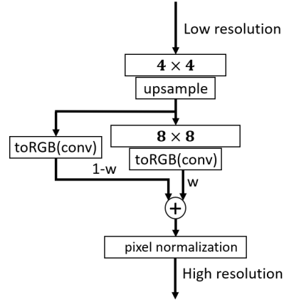
Figure 2 shows the architecture of a layer in PG-GAN which includes several different functions. Given a low-resolution input from upstream layers, we do upsampling, convolutions (Krizhevsky et al. (2012)), and weighted residual connection He et al. (2016). Finally, a pixel normalization Kurach et al. (2019) which is a type of avoids the competing gradient magnitudes spiraling out of control is imposed on the output as
| (1) |
where is the number of channels, and are the original and normalized feature vector at pixel and . And refers to normalizing coefficients which implements the pixel normalization.
The progressive growing strategy gradually appends new layers to the network, organizing layers into different granularity levels. Given a random input and the PG-GAN generator , we have the generated image and is a set of units (i.e., channels in convolution operations) in a given middle layer which are closely related to classes of objects respectively. Literature shows that while units in the middle layers (layer4 to layer7 in PG-GAN) relate to object-level concepts (e.g. chairs, painting), they in layers ahead relate to background concepts (e.g. ceiling, sky) and in latter layers focus on abstract concepts (e.g. color, texture). In this work, to enable detailed analysis over objects’ disentanglement properties, we constrain our training and following experiments of PG-GAN on the LSUN (Yu et al. (2015)) conference room dataset.
PG-GAN’s ability to yield various fine-grained objects is critical for analyzing disentanglement between different objects. In the literature, researchers conduct a wide range of experiments to primarily show that PG-GAN exhibits both disentangled and entangled properties in different scenarios. Especially in (Bau et al. (2018)), the authors present a series of qualitative unit-level experiments to show that in the unit-ablation transformation, while in some cases the PG-GAN shows disentanglement (such as ablating paintings on the wall), in other cases, entangled phenomena are observed, mainly categorized into two types including unsuppressible and emerged objects after ablation. In this work, we try to provide deeper thoughts about the disentanglement caused by function-level and mutual relationships between objects and eventually explain the above unexpected entanglement.
3 Problem Definition
Intuitively, the disentanglement of deep models denotes the scenario that a transformation operating on a local component does not disturb other components in the same figure. A rigorous definition of transformation disentanglement is proposed by Besserve et al. (2018a), which is presented as below:
Literature Definition (Counterfactual-based Disentanglement).
Given a transformation on the data manifold, it is disentangled on a generative model with respect to a subset of the generated outcome, if there is a transformation acting on internal representation units such that for any endogenous value
| (2) |
where only affects variables indexed by .
This definition points out that a transformation is disentangled if and only if ’s effect corresponds to an internal transformation which only causes changes on , a specific outcome subset. In this research, we specify in the above definition as the unit-ablation transformation, which is denoted by . Therefore, denotes the transformation directly ablating objects, while is the transformation ablating input units. We further define to the area of a specific object class on the generated image. We also notice that is disentangled if and only if there is disentangled. Therefore, in the rest of the paper, we use “disentanglement” for short to represent the disentangled property of the ablation transformation .
The above definition allows us to examine whether a type of objects are disentangled under the unit-ablation transformation on PG-GAN generated figures. For example, given a GAN , if the on chair objects area is disentangled, we expect to find a internal transformation acting on units leading to only and sufficient disappearance of chair objects in the generated image. Therefore, we have the following definition of the disentanglement of a class of objectives.
Definition 1 (The Disentanglement of a Set of Objects).
A class of objectives is disentangled under the ablation transformation , if the unit-ablation transformation acting on satisfies
| (3) |
where only affects variables indexed by .
The above definition also suggest that the disentanglement of an object is influenced by several factors, among which the features of units have the most direct and apparent effect because directly acts on . To quantitatively identify units ’s impact on the appearance of a specific class of objects, following (Bau et al. (2018)) and (Holland, 1988), we leverage a standard causal metric—the average causal effect (ACE) to reflect a unit’s effect on disentanglement.
Definition 2 (Unit’s Effect on Disentanglement).
For any possible and , the ACE of unit set on object class is defined as
| (4) |
where is the image with ablated at and is the image with inserted at .
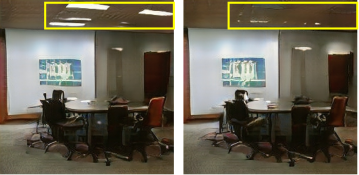
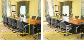
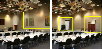
Note that the is the expectation over all the possible , which reflects the average effect of units on the object class in any scenarios. In Figure 3, we exhibit the three types of disentangled and entangled phenomena caused by ablating units with top-. The first sample shows a fully disentangled behavior (as the paintings on the wall disappear), but the second and third exhibit entangled phenomena. In the second one, although top- chair units are ablated, the chair objects are not ablated in the outcome, with only sizes shrinking a little bit. In the third one, while paintings are removed, new objects such as doors unexpectedly emerge.
Literature has suggested that in the internal components of neural networks may have roles in causing entanglement (Besserve et al., 2018b; Chen et al., 2018). In this work, we propose to study the pixel normalization function’s effect on disentanglement via experimental designs. We define it as follows:
Definition 3 (Pixel Normalization’s Effect on Disentanglement).
Given an input , let denote ablated units, denote pixel normalization function’s effect, and denote other functions’ effect, there is
| (5) |
where refers to the functions and units’ joint effect on . Consequently, the effect of pixel normalization given the ablation transformation could be represented by
| (6) |
Since the pixel normalization acts on the units, ’s behavior is probably influenced by the aggregating properties of the input and corresponding . More specifically,
Definition 4 (Distribution and Ranking (Informal)).
With a set of object classes and the set of units , we informally define:
1) distribution of : given an object class and for every unit , the density distribution of
2) ranking of : for every , the ranking sequence of their
4 Method: Difference-in-Difference experiment design
To bridge the pixel normalization to disentanglement, in Section 3 we propose to identify which represents pixel normalization’s universal effect, and then to explore how the properties of will influence ’s form of expression. For the first problem, we introduce a counterfactual-based Difference-in-Difference (DID) (Ciani & Fisher, 2018) experiment framework; for the second, based on the different-in-different approach, we compare under four scenarios with different unit distributions and rankings.
4.1 Counterfactual DID experiments for identifying function’s effect
We argue that the pixel normalization’s transformation has a significant impact on disentanglement of the . The intuition is that, from Equation 1, we know that will increase when there are units ablated (i.e. ), leading to augmentations on un-ablated units. In previous study, researcher show the object-level generation of PG-GAN is determined by the 4-layer to 13-layer in PG-GAN. Therefore, in order to investigate how the affects the transformation , we propose to control the in these 10 layers for constructing counterfactuals.
Naturally, we have a factual experiment as shown in Equation 7. To show ’s effect on the transformation , we construct a counterfactual case where and remains controlled. Technically speaking, this control is performed by enforcing normalizing coefficients in 4-layer to 13-layer to be the same as the original situation with . For another factual experiment , we conduct the same control as enforcing coefficients to be the same to reveal ’s impact on . As a result, we construct two pairs of counterfactual experiments for difference in difference analysis as follow:
| (7) | |||
and therefore the real effect could be computed as:
| (8) | ||||
which indicates the real effect of pixel normalization effect function imposed on the image. Noted that this effect is also unbiased because the unrelated effect has been offset in the difference.
4.2 Scenario-conditioned experiments for unit distribution and ranking
Difference-in-Difference experiments enable us to systematically analyze pixel normalization’s effects on disentanglement of any given objects on given images. But we may still not explain the unexpected evidences in Figure 3, that with the same application of pixel normalization, different object classes, or the same object class in different scenarios show significant entangled properties.
Therefore, in this step of experiment, we design to compare the DID experiment results conditioned on its distribution of and ranking of . More specifically, we categorized them into types:
-
1.
distribution of : 1) units symmetrically locate in both high-ACE and low-ACE area, 2) units concentrate in high-ACE area.
-
2.
ranking of : 1) the top ranking object’s ACE overwhelms the second one, 2) the top ranking object marginally surpasses the second one.
Although theoretically we have 4 scenarios, in fact we will show that given the symmetrical distribution condition, the ranking of does not take effect, leaving only 3 meaningful cases.
5 Result
5.1 Pixel normalization’s effect: entangle objects by in-painting
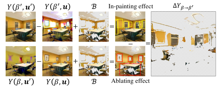
Our experiments demonstrate a strong tie between pixel normalization and the entanglement in the object ablation transformation . Supported by difference-in-difference counterfactual experiments, we discover that the pixel normalization’s effect , informally, is to in-paint objects to ablated areas on the generated image caused by the internal ablation of corresponding units, which consequently leads to entanglement in PG-GAN. In Figure 4, we present the mechanism of how pixel normalization causes entanglement. Recall the difference-in-difference definition of pixel normalization’s effect as:
| (9) |
of which the first term describes the in-painting effect produced by (first two columns of Row 1) and the second term depicts an ablation effect (first two columns of Row 2). As a consequence of their difference, the in-painted area will cover the ablation area and presents a joint effect of in-painting. In order to well present the in-painting effect and ablation effect, we present the two effects on a background figure . The background figure presents the areas that do not significantly change by both effects. The background figure is presented on the third column of Figure 4.
In-painting effect under (after ablation) When is controlled, from to its counterfactual , pixel normalization shows its in-painting functionality by inserting door objects on the original wall and wall objects on where the paintings are.
Ablation effect under (before ablation) When is controlled, pixel normalization’s response is to ablate the area of all objects related to the removed units. For example, in Figure 4’s lower row where we ablated units mainly contribute to the paintings, from the original case to the counterfactual case , the PG-GAN removes all paintings away together with surrounding wall areas and turning them into a yellow background.
Joint DID effect of the pixel normalization Combining the above two effects of in-painting and ablation, we present the final DID joint effect as in the rightmost subfigure in Figure 4, which clearly illustrates that the pixel normalization in-paints not only walls at where the paintings are ablated, unexpected door objects are also inserted to places where should have been wall. Without the rigorous DID experimental design, one may only notice the effect from the original case to the natural ablation case , and thus ignore the complicated mechanisms behind the pixel normalization.
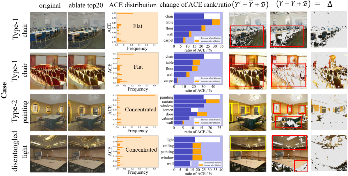
5.2 What to in-paint: unit distribution and ranking
In Section 5.1, we have answered the universal effect of pixel normalization, that to in-paint the area affected by the ablation transformation. But what objects the pixel normalization will in-paint to the area and how intensive this in-painting will remain unclear. We argue that the form of in-painting the pixel normalization will present in an ablation transformation could be identified according to the properties of units’ ACE , namely the distribution and the ranking.
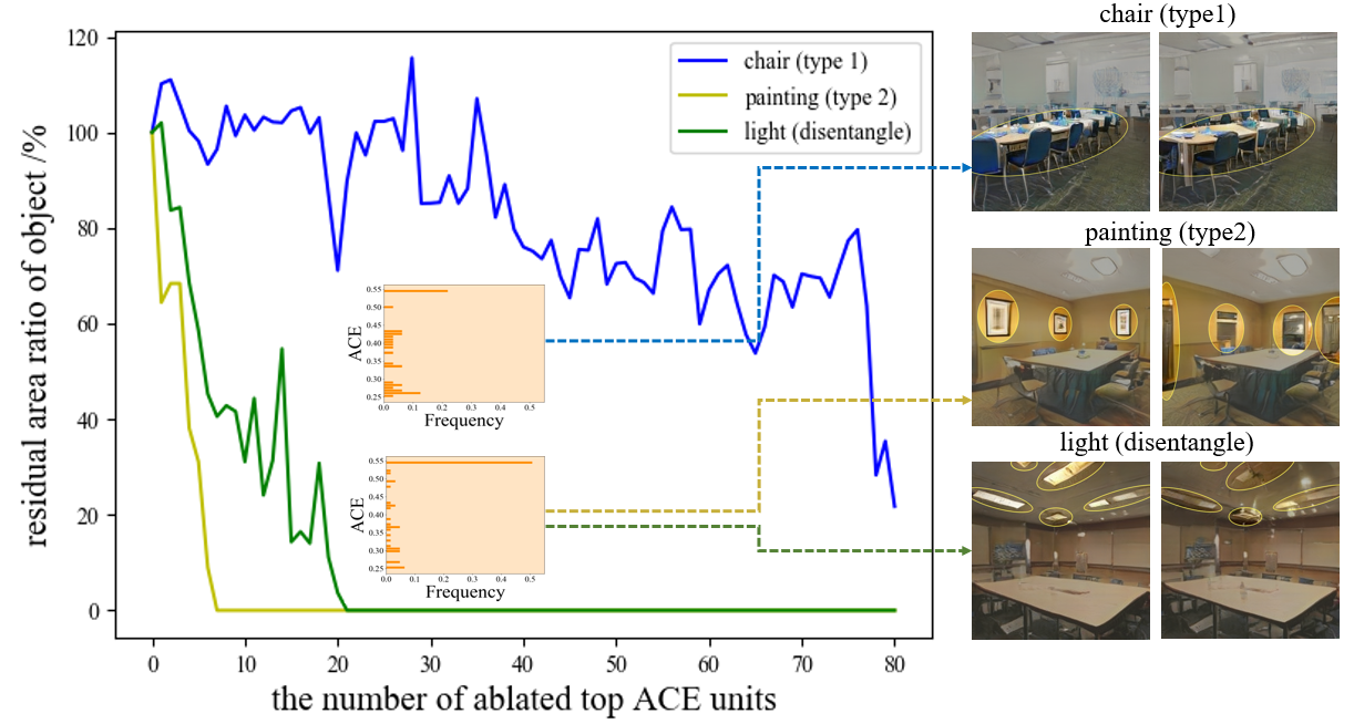
First, the distribution of determines whether an object class could be ablated. In Figure 5, we select three typical types of object classes, including chair, painting and light, to illustrate how the ACE distribution directly determines an object’s ability to be disentangled. We ablate the units with ACE ranking from top to down, and observe an apparent gap between chair (categorized as Type-1) objects and painting & light (categorized as Type -2 & disentangled). While the chairs’ area remains stubborn with top-80 ACE units ablated, the painting and light objects take no more than 20 of the top ACE units ablated to be eliminated.
This confusing phenomenon could be explained when we look into their distribution of ACE. We observe that Type-1 classes distribution is flat, with high-ACE units explains for no more than 50% of the total effect. Therefore, when we removing high-ACE units, the loss of their effects could be compensated by those lower-ACE units with ’s augmentation. However, on the contrary, Type-2 and disentangled classes have a concentrated distribution where influential units dominantly locate at the high-ACE part and thus make the most contributions to the object generation. To conclude, with such flat distribution, Type-1 classes are not disentangled at all with the ablation transformation.
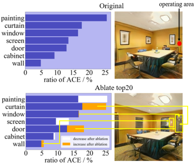
Second, given the Type-2 and disentangled object classes, ablation on corresponding units could eliminate them. But for Type-2 classes, when we compare it with those disentangled ones, we observe mis-ablation phenomena in which other unexpected objects would emerge. To explain this, based on the concentrated unit distribution we consider the influence of the ranking of units as shown in Figure 6. When we operate ablation on the red point and examine its unit ranking, before ablation ACE for painting is the largest, but ACE for window, curtain and door are also quite large. After ablation, the decrease of painting ACE and the increase of wall ACE make painting removed and replaced with wall. Moreover, ACE for curtain, door and window become the largest and they indeed appear in the area around the operation point, which successfully explains the mis-ablation.
For the disentangled classes, such as the lights we display in the summary plot Figure 1, they actually share a similar ranking of units with those of Type-2. The only difference is that the second candidate unit just behind the ablated one happens to be the original surrounding.
 \setcaptionwidth
2.8in
 \setcaptionwidth
2.0in
6 Conclusion
We in this research propose a difference-in-difference (DID) counterfactual framework to design experiments for acquiring insights into the black box of PG-GAN transformation and analyzing the entanglement mechanism in one of the Progressive-growing GAN (PG-GAN). Our experiment clarifies the mechanism of how pixel normalization causes PG-GAN entanglement during an input-unit-ablation transformation. We discover that pixel normalization causes object entanglement by in-painting the area occupied by ablated objects. We also discover the unit-object relation determines whether and how pixel normalization causes object entanglement. Our DID framework theoretically guarantees that the mechanisms that we discover is solid, explainable, and comprehensive.
References
- Abadie (2005) Alberto Abadie. Semiparametric difference-in-differences estimators. The Review of Economic Studies, 72(1):1–19, 2005.
- Athey & Imbens (2006) Susan Athey and Guido W Imbens. Identification and inference in nonlinear difference-in-differences models. Econometrica, 74(2):431–497, 2006.
- Bau et al. (2017) David Bau, Bolei Zhou, Aditya Khosla, Aude Oliva, and Antonio Torralba. Network dissection: Quantifying interpretability of deep visual representations. In Proceedings of the IEEE conference on computer vision and pattern recognition, pp. 6541–6549, 2017.
- Bau et al. (2018) David Bau, Jun-Yan Zhu, Hendrik Strobelt, Bolei Zhou, Joshua B Tenenbaum, William T Freeman, and Antonio Torralba. Gan dissection: Visualizing and understanding generative adversarial networks. In ICLR, 2018.
- Besserve et al. (2018a) Michel Besserve, Arash Mehrjou, Rémy Sun, and Bernhard Schölkopf. Counterfactuals uncover the modular structure of deep generative models. arXiv preprint arXiv:1812.03253, 2018a.
- Besserve et al. (2018b) Michel Besserve, Rémy Sun, and Bernhard Schölkopf. Intrinsic disentanglement: an invariance view for deep generative models. In ICML 2018 Workshop on Theoretical Foundations and Applications of Deep Generative Models, 2018b.
- Chen et al. (2018) Ricky TQ Chen, Xuechen Li, Roger B Grosse, and David K Duvenaud. Isolating sources of disentanglement in variational autoencoders. In Advances in Neural Information Processing Systems, pp. 2610–2620, 2018.
- Chen et al. (2016) Xi Chen, Yan Duan, Rein Houthooft, John Schulman, Ilya Sutskever, and Pieter Abbeel. Infogan: Interpretable representation learning by information maximizing generative adversarial nets. In Advances in neural information processing systems, pp. 2172–2180, 2016.
- Ciani & Fisher (2018) Emanuele Ciani and Paul Fisher. Dif-in-dif estimators of multiplicative treatment effects. Journal of Econometric Methods, 2018.
- Goodfellow et al. (2014) Ian Goodfellow, Jean Pouget-Abadie, Mehdi Mirza, Bing Xu, David Warde-Farley, Sherjil Ozair, Aaron Courville, and Yoshua Bengio. Generative adversarial nets. In Advances in neural information processing systems, pp. 2672–2680, 2014.
- Goodman-Bacon (2018) Andrew Goodman-Bacon. Difference-in-differences with variation in treatment timing. Technical report, National Bureau of Economic Research, 2018.
- He et al. (2016) Kaiming He, Xiangyu Zhang, Shaoqing Ren, and Jian Sun. Deep residual learning for image recognition. In Proceedings of the IEEE conference on computer vision and pattern recognition, pp. 770–778, 2016.
- Higgins et al. (2016) Irina Higgins, Loic Matthey, Arka Pal, Christopher Burgess, Xavier Glorot, Matthew Botvinick, Shakir Mohamed, and Alexander Lerchner. beta-vae: Learning basic visual concepts with a constrained variational framework. 2016.
- Holland (1988) Paul W Holland. Causal inference, path analysis and recursive structural equations models. ETS Research Report Series, 1988(1):i–50, 1988.
- Imbens & Rubin (2015) Guido W Imbens and Donald B Rubin. Causal inference in statistics, social, and biomedical sciences. Cambridge University Press, 2015.
- Karpathy et al. (2015) Andrej Karpathy, Justin Johnson, and Li Fei-Fei. Visualizing and understanding recurrent networks. arXiv preprint arXiv:1506.02078, 2015.
- Karras et al. (2017) Tero Karras, Timo Aila, Samuli Laine, and Jaakko Lehtinen. Progressive growing of gans for improved quality, stability, and variation. arXiv preprint arXiv:1710.10196, 2017.
- Krizhevsky et al. (2012) Alex Krizhevsky, Ilya Sutskever, and Geoffrey E Hinton. Imagenet classification with deep convolutional neural networks. In Advances in neural information processing systems, pp. 1097–1105, 2012.
- Kulkarni et al. (2015) Tejas D Kulkarni, William F Whitney, Pushmeet Kohli, and Josh Tenenbaum. Deep convolutional inverse graphics network. In Advances in neural information processing systems, pp. 2539–2547, 2015.
- Kurach et al. (2019) Karol Kurach, Mario Lučić, Xiaohua Zhai, Marcin Michalski, and Sylvain Gelly. A large-scale study on regularization and normalization in gans. In International Conference on Machine Learning, pp. 3581–3590. PMLR, 2019.
- Olah et al. (2018) Chris Olah, Arvind Satyanarayan, Ian Johnson, Shan Carter, Ludwig Schubert, Katherine Ye, and Alexander Mordvintsev. The building blocks of interpretability. Distill, 3(3):e10, 2018.
- Pearl (2009) Judea Pearl. Causality. Cambridge university press, 2009.
- Radford et al. (2015) Alec Radford, Luke Metz, and Soumith Chintala. Unsupervised representation learning with deep convolutional generative adversarial networks. arXiv preprint arXiv:1511.06434, 2015.
- Schwab & Karlen (2019) Patrick Schwab and Walter Karlen. Cxplain: Causal explanations for model interpretation under uncertainty. In Advances in Neural Information Processing Systems, pp. 10220–10230, 2019.
- Selvaraju et al. (2017) Ramprasaath R Selvaraju, Michael Cogswell, Abhishek Das, Ramakrishna Vedantam, Devi Parikh, and Dhruv Batra. Grad-cam: Visual explanations from deep networks via gradient-based localization. In Proceedings of the IEEE international conference on computer vision, pp. 618–626, 2017.
- Simonyan et al. (2013) Karen Simonyan, Andrea Vedaldi, and Andrew Zisserman. Deep inside convolutional networks: Visualising image classification models and saliency maps. arXiv preprint arXiv:1312.6034, 2013.
- Yu et al. (2015) Fisher Yu, Ari Seff, Yinda Zhang, Shuran Song, Thomas Funkhouser, and Jianxiong Xiao. Lsun: Construction of a large-scale image dataset using deep learning with humans in the loop. arXiv preprint arXiv:1506.03365, 2015.
- Zhang et al. (2019) Han Zhang, Ian Goodfellow, Dimitris Metaxas, and Augustus Odena. Self-attention generative adversarial networks. In International Conference on Machine Learning, pp. 7354–7363. PMLR, 2019.
- Zhou et al. (2018) Bolei Zhou, Yiyou Sun, David Bau, and Antonio Torralba. Interpretable basis decomposition for visual explanation. In Proceedings of the European Conference on Computer Vision (ECCV), pp. 119–134, 2018.