Deep and Interpretable Regression Models for Ordinal Outcomes

Abstract

Outcomes with a natural order commonly occur in prediction tasks and often the available input data are a mixture of complex data like images and tabular predictors. Deep Learning (DL) models are state-of-the-art for image classification tasks but frequently treat ordinal outcomes as unordered and lack interpretability. In contrast, classical ordinal regression models consider the outcome’s order and yield interpretable predictor effects but are limited to tabular data. We present ordinal neural network transformation models (ontrams), which unite DL with classical ordinal regression approaches. ontrams are a special case of transformation models and trade off flexibility and interpretability by additively decomposing the transformation function into terms for image and tabular data using jointly trained neural networks. The performance of the most flexible ontram is by definition equivalent to a standard multi-class DL model trained with cross-entropy while being faster in training when facing ordinal outcomes. Lastly, we discuss how to interpret model components for both tabular and image data on two publicly available datasets.

Keywords

deep learning, interpretability, distributional regression, ordinal regression, transformation models

1 Introduction

Many classification problems deal with classes that show a natural order. This includes for example patient outcome scores in clinical studies or movie ratings (Oghina et al., 2012). These ordinal outcome variables may not only depend on interpretable tabular predictors like age or temperature but also on complex input data such as medical images, networks of public transport, textual descriptions, or spectra. Depending on the complexity of the input data and the concrete task, different analysis approaches have established to tackle the ordinal problems.

Ordinal regression as a probabilistic approach has been studied for more than four decades (McCullagh, 1980). The goal is to fit an interpretable regression model, which estimates the conditional distribution of an ordinal outcome variable $Y$ based on a set of tabular predictors. The ordinal outcome $Y$ can take values in a set of ordered classes and the tabular predictors are scalar and interpretable like age. Ordinal regression models make use of the information contained in the order of the outcome and provide a valid probability distribution instead of a single point estimate for the most likely outcome. This is essential to reflect uncertainty in the predictions. Moreover, the estimated model parameters are interpretable as the effect a single predictor has on the outcome given the remaining predictors are held constant. This allows experts to assess whether the model corresponds to their field knowledge and provides the necessary trust for application in critical decision making. However, there is a trade-off between interpretability and model complexity. The higher the complexity of a model, the harder it becomes to directly interpret the individual model parameters.

Deep Learning (DL) approaches have gained huge popularity over the last decade and achieved outstanding performances on complex tasks like image classification and natural language processing (Goodfellow et al., 2016). The models take the raw data as input and learn relevant features during the training procedure by transforming the input into a latent representation, which is suitable to solve the problem at hand. This avoids the challenging task of feature engineering, which is necessary when working with statistical models. Yet, unlike statistical models, most DL models have a black box character, which makes it hard to interpret individual model components. In addition, ordinal outcomes in DL approaches are frequently modeled in the same way as unordered outcomes using multi-class classification (MCC). That is, softmax is used as the last-layer activation and the loss function is the categorical cross-entropy. In this setting, solely the probability assigned to the true class is entering the loss function, which ignores the outcome’s natural order.

To the best of our knowledge, there is currently no ordinal DL model, which enables to integrate tabular predictors and yields interpretable effect estimates for the tabular and the image data. This is a major disadvantage for example in fields like medicine which requires multiple data modalities for decision making but also a reliably interpretable model which quantifies the effects of the predictors on the outcome (Rudin, 2019).

1.1 Our Contribution

In this work we introduce ordinal neural network transformation models (ontrams), which unite classical ordinal regression with DL approaches while conserving the interpretability of statistical and flexibility of DL models. We use a theoretically sound maximum-likelihood based approach and reparametrize the categorical cross-entropy loss to incorporate the order of the outcome. This guarantees the estimation of a valid probability distribution. By definition, the reparameterized negative log-likelihood (NLL) loss is able to achieve the same prediction performance as a standard DL model trained with cross-entropy loss, but allows a faster training in case of an ordinal outcome. The main advantage of the proposed ontrams is that ontrams provide interpretable effect estimates for the different input data, which is not possible with other DL models.

We view ordinal regression models from a transformation model perspective (Hothorn et al., 2014; Sick et al., 2021). This change of perspective is useful because it allows a holistic view on regression models, which easily extends beyond the case of ordinal outcomes. In transformation models the problem of estimating a conditional outcome distribution is translated into a problem of estimating the parameters of a monotonically increasing transformation function, which transforms the potentially complex outcome distribution to a simpler, predefined distribution $F_{Z}$ of a continuous variable.

The goal of ontrams is to estimate a flexible outcome distribution based on a set of predictors including images and tabular data while keeping components of the model interpretable. ontrams are able to seamlessly integrate both types of data with varyingly complex interactions between the two, by taking a modular approach to model building. The data analyst can choose the scale on which to interpret image and tabular predictor effects, such as the odds or hazard scale, by specifying the simple distribution function $F_{Z}$. In addition, the data analyst has full control over the complexity of the individual model components. The discussed ontrams will contain at most three (deep) neural networks for the intercepts in the transformation function, the tabular and the image data. Together with the simple distribution function $F_{Z}$ the output of these neural networks will be used to evaluate the NLL loss. In the end, the NNs, which control the components of the model, are jointly fit by standard deep learning algorithms based on stochastic gradient descent. In this work, we feature convolutional neural networks (CNNs) for complex input data like images. However, the high modularity of ontrams enables many more applications such as recurrent neural networks for text-based models.

1.2 Organization of this Paper

We first describe the necessary theoretical background of multi-class classification and ordinal regression. Afterwards, an outline of related work is given in Section 2.3 to highlight the contributions of ontrams to the field. We then provide details about ontrams in Section 3. Subsequently, we describe the data sets, experiments, and models we use to study and benchmark ontrams (Section 4). We end this paper with a discussion of our results and juxtaposition of the different approaches in light of model complexity, interpretability, and predictive performance. We present further results in Appendix B and complement our discussion of different loss functions and evaluation metrics in Appendices D and E, respectively. Because most state-of-the-art approaches to ordinal outcomes are classifiers, we particularly highlight the distinction between ordinal classification and the proposed regression approach of ontrams in Appendix F.

2 Background

First, we will describe the multi-class classification approach frequently applied in deep learning, which will serve as a baseline model in our experiments. We outline cumulative ordinal regression models as the statistical approach to ordinal regression and how they can be viewed as a special case of transformation models. In the end we summarize related work in the field of deep ordinal regression and classification and interpretable machine learning.

2.1 Multi-class Classification

Deep learning prediction models for multi-class classification (MCC) are based on a NN whose output layer contains $K$ units and uses a softmax as the last-layer activation function to predict a probability for each class. The softmax function is defined as

$$p_{k}=\operatorname{softmax}(s_{k})=\frac{\exp(s_{k})}{\sum_{j=1}^{K}\exp(s_{j})},$$ (1)

where $s_{k}$ is the value of unit $k$ before applying the activation function. Typically, a MCC model is trained by minimizing the categorical cross-entropy loss. The categorical cross-entropy is computed over $n$ samples by

$$\text{CE}:=-\sum_{i=1}^{n}\sum_{k=1}^{K}y_{ki}\log\mathbb{P}(Y=y_{ki}\rvert\boldsymbol{x}_{i})=-\sum_{i=1}^{n}\log\mathcal{L}_{i},$$ (2)

with $y_{ki}$ being entry $k$ of the one-hot-encoded outcome for input $\boldsymbol{x}_{i}$, which is one for the observed class and zero otherwise. The probability for the observed class is the likelihood contribution $\mathcal{L}_{i}$ of the $i$th observation. It is well known that the cross-entropy loss is equivalent to the negative log-likelihood for multinomial outcome variables (see Figure 1 A and B). Moreover, Eq. (2) highlights that the likelihood is a local measure because solely the predicted probability for the observed class contributes to the loss. That is, in case of ordinal outcomes, the outcome’s natural order is ignored. Note that MCC models as defined above are referred to as multinomial regression in the statistical literature, highlighting the fact that they predict an entire probability distribution instead of a single class (see Appendix F).

2.2 Ordinal Regression Models

Ordinal regression aims to characterize the whole conditional distribution of an ordinal outcome variable given its predictors. A discussion of ordinal regression and how they can be viewed as transformation models is given in the following.

2.2.1 Cumulative Ordinal Regression Models

The goal of the statistical approach to ordinal regression is mainly to develop an interpretable model for the conditional distribution of the ordered outcome variable $Y$ with $K$ possible values $y_{1}<y_{2}<\dots<y_{K}$. Before discussing how interpretable model components are achieved, we discuss the question of how the order of the outcome can be taken into account.

The distribution of an outcome variable is fully determined by its probability density function (PDF). For an ordinal outcome the PDF describes the probabilities of the different classes, which is equivalent to the PDF of an unordered outcome. Yet, unlike an unordered outcome an ordered outcome possesses a well defined cumulative distribution function (CDF) $F_{Y}$, which naturally contains the order. The CDF $F_{Y}(y_{k})=\mathbb{P}(Y\leq y_{k})$ is a step function, which takes values between zero and one and describes the probability of an outcome $Y$ of being smaller or equal to a specific class. The steps are positioned at $y_{k}$, $k=1,\dots,K$ and the heights of the steps correspond to the probability $\mathbb{P}(Y=y_{k})=F_{Y}(y_{k})-F_{Y}(y_{k-1})=:\mathcal{L}_{i}$ of observing class $k$ (cf. Figure 1 A and B). As indicated in the previous subsection, the likelihood contribution for an observation $(y_{ki},\boldsymbol{x}_{i})$ is given by the predicted probability for the observed class, which can be rewritten as

$$\mathcal{L}_{i}=\mathbb{P}(Y=y_{ki}\rvert\boldsymbol{x}_{i})=\mathbb{P}(Y\leq y_{ki}\rvert\boldsymbol{x}_{i})-\mathbb{P}(Y\leq y_{(k-1)i}\rvert\boldsymbol{x}_{i}),$$ (3)

for $k=1,\dots,K-1$ and $\mathbb{P}(Y\leq y_{0}):=0$, $\mathbb{P}(Y\leq y_{K})=1$. Parametrizing the likelihood contributions using the CDF directly enables to incorporate the order of the outcome when formulating regression models for ordinal data (Section 3). It is worth noting that the loss is still the same negative log likelihood as in eq. (2) merely using a different parametrization to take the outcome’s natural order into account.

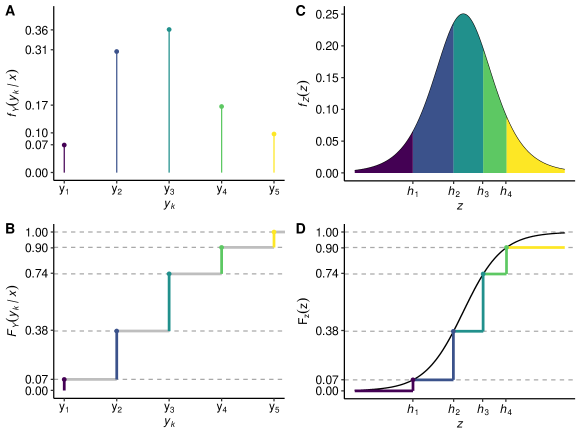
Figure 1: Density and distribution function for an ordered outcome with five classes. (A) The probability density function (PDF) describes the probability of the outcome belonging to class $k$. (B) The cumulative distribution function (CDF) describes the probability of the outcome belonging to any class below and including class $k$. The heights of the steps correspond to the probability of belonging to class $k$, which are given by the PDF. Panels C and D depict the PDF and CDF of the latent variable $Z$ and illustrate the equivalence between modelling on the scale of $Y$ and $Z$. For brevity the cut points are denoted by $h_{k}:=h(y_{k}\rvert\boldsymbol{x})$. Note that $h_{5}=+\infty$ gives rise to the yellow area corresponding to the conditional probability of $Y$ belonging to the fifth class, but does not show on the $x$-axis in panels C and D.

Many ordinal regression models assume the existence of an underlying continuous latent variable (an unobserved quantity) $Z$. Sometimes field experts can give an interpretation for the latent variable $Z$, e.g., the degree of illness of a patient. The ordinal outcome variable $Y$ is understood as a categorized version of $Z$ resulting from incomplete knowledge; we only know the classes in terms of the intervals in which $Z$ lies. Fitting an ordinal regression model based on the latent variable approach aims at finding cut points $h(y_{k}\rvert\boldsymbol{x})$ at which $Z$ is separated into the assumed classes (see Figure 1 C). This is done by setting up a monotonically increasing step function $h$ that transforms the ordinal class values into cut points that retain the order (see Figure 2). Even if $Z$ can not be interpreted directly, using a latent variable approach has advantages, because the chosen distribution of $Z$ determines the interpretability of the terms in the transformation function (see section 2.2.2).

Moreover, the latent variable approach enables to understand ordinal regression as a special case of parametric transformation models, which were recently developed in statistics (Hothorn et al., 2014) and are applicable to a wide range of outcomes with natural extensions to classical machine learning techniques such as random forests and boosting. Transformation models are able to model highly flexible outcome distributions while simultaneously keeping specific model components interpretable. In transformation models the conditional outcome distribution of $(Y\rvert\boldsymbol{x})$ is modeled by transforming the outcome variable $(Y\rvert\boldsymbol{x})$ to a variable $(Z\rvert\boldsymbol{x})$ with known (simple) CDF $F_{Z}$, like the Gaussian or logistic distribution. Transformation models in general are thus defined by

$$F_{Y}(y\rvert\boldsymbol{x})=F_{Z}(h(y\rvert\boldsymbol{x})),$$ (4)

and all models in our proposed framework of ontrams are of this form.

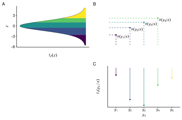
Figure 2: Transformation model likelihoods for a model with ordinal outcome. Panel C shows the conditional density of $Y$ given $\boldsymbol{x}$, which gets mapped onto the density of the latent variable $Z$ (A) via the transformation function $h$ (B). The likelihood contributions are in fact probabilities and given by the area under the density of $Z$ between two consecutive cut points in the transformation function. Note that $h(y_{5}\rvert\boldsymbol{x})=+\infty$ does not show on the plot for the transformation function, but is evident from the yellow area under the density of $Z$.

The first step to set up an ordinal transformation model is to choose a continuous distribution for $Z$, which determines the interpretational scale of the effect of a predictor on the outcome (see Section 2.2.2). The goal is then to fit a monotonically increasing transformation function $h$, which maps the observed outcome classes $(y_{k}\rvert\boldsymbol{x})$ to the conditional cut points

$$h(y_{k}\rvert\boldsymbol{x}),\;k=1,\dots,K-1,$$ (5)

of the latent variable $Z$, as illustrated in Figure 2. In the example in Figure 2 the outcome can take five classes and the $K-1$ cut points $h(y_{1}\rvert\boldsymbol{x})$, $h(y_{2}\rvert\boldsymbol{x})$, $h(y_{3}\rvert\boldsymbol{x})$, and $h(y_{4}\rvert\boldsymbol{x})$ have to be estimated. The first class of $Y$ on the scale of $Z$ is given by the interval $(-\infty,h(y_{1}\rvert\boldsymbol{x})]$, the fifth class as $(h(y_{4}\rvert\boldsymbol{x}),+\infty)$, so often the conventions $h(y_{0}\rvert\boldsymbol{x})=-\infty$ and $h(y_{K}\rvert\boldsymbol{x})=+\infty$ are used. The likelihood contribution of a given observation $(y_{ki},\boldsymbol{x}_{i})$ can now be derived from the CDF of $Z$ instead of $Y$ and is given by

$$\mathcal{L}_{i}(h;y_{ki},\boldsymbol{x}_{i}) =\mathbb{P}(Y=y_{ki}\rvert\boldsymbol{x}_{i})$$

$$=F_{Y}(y_{ki}\rvert\boldsymbol{x}_{i})-F_{Y}(y_{(k-1)i}\rvert\boldsymbol{x}_{i})$$

$$=F_{Z}(h(y_{ki}\rvert\boldsymbol{x}_{i}))-F_{Z}(h(y_{(k-1)i}\rvert\boldsymbol{x}_{i})).$$ (6)

The single likelihood contributions are the heights of the steps in the CDF or equivalently the area under the density of the latent variable $Z$ between two consecutive cut points (cf. Figure 2 B, C). Note that two consecutive cut points enter the likelihood, such that the natural order of the outcome is used to parametrize the likelihood, although the likelihood contribution is given by the probability of the observed class alone. Consequently, minimizing the negative log-likelihood

$$-\ell(h;y_{1:n},\boldsymbol{x}_{1:n})=-\sum_{i=1}^{n}\log\mathcal{L}_{i}(h;y_{ki},\boldsymbol{x}_{i})$$ (7)

estimates the conditional outcome distribution of $(Y\rvert\boldsymbol{x})$ by estimating the unknown parameters of the transformation function, which in our application are the cut points of $Z$. Note that in principle this formulation allows us to directly incorporate uncertain observations, for instance, an observation may lie somewhere in $[y_{k},y_{k+2}]$, $k\leq K-2$ if a rater is uncertain about the quality of a wine or a patient rates their pain in between two classes.

2.2.2 Interpretability in Proportional Odds Models

The interpretability of a transformation model depends on the choice of the distribution $F_{Z}$ of the latent variable $Z$ and the transformation function $h$. A summary of common interpretational scales is given in Table 1.

Table 1: Interpretational scales of shift terms induced by $F_{Z}$ (Tutz, 2011). Most link functions have been studied in the context of proportional odds model neural networks and a classification loss (Vargas et al., 2020). More details concerning the interpretational scales are given in Appendix C.

$F_{Z}$	$F_{Z}^{-1}$	Symbol	Interpretation of shift terms
Logistic	$\operatorname{logit}$	$F_{\operatorname{L}}$	log odds-ratio
Gompertz	cloglog	$F_{\operatorname{MEV}}$	log hazard-ratio
Gumbel	loglog	$F_{\text{Gumbel}}$	log hazard-ratio for $Y_{r}=K+1-Y$
Normal	probit	$\Phi$	not interpretable directly

Here, we demonstrate interpretability through the example of a proportional odds model, which is well known in statistics (Tutz, 2011). For the distribution of $Z$ we choose the standard logistic distribution (denoted by $F_{\operatorname{L}}$), whose CDF is given by $F_{Z}(z)=F_{\operatorname{L}}(z):=(1+\exp(-z))^{-1}$. The transformation function $h$ is parametrized as

$$h(y_{k}\rvert\boldsymbol{x})=\vartheta_{k}-\sum_{j=1}^{J}\beta_{j}x_{j}=\vartheta_{k}-\boldsymbol{x}^{\top}\text{\boldmath$\beta$},\;j=1,\dots,J.$$ (8)

A transformation model with such a transformation function is called linear shift model, since a change $\Delta x_{j}$ in a single predictor $x_{j}$ causes a linear shift of size $\beta_{j}\Delta x_{j}$ in the transformation function. In Figure 3 this is visualized for an outcome $y_{k}$ depending on a single predictor $x$, which is increased by one unit (here from 0 to 1). This increase results in a simple shift of size $\beta$ in the transformation function (Figure 3 B). However, the resulting conditional distribution changes in a more complex way (Figure 3 A). Note that the shape of the transformation function $h$ does not depend on $x$ and stays unchanged while it is shifted downwards.

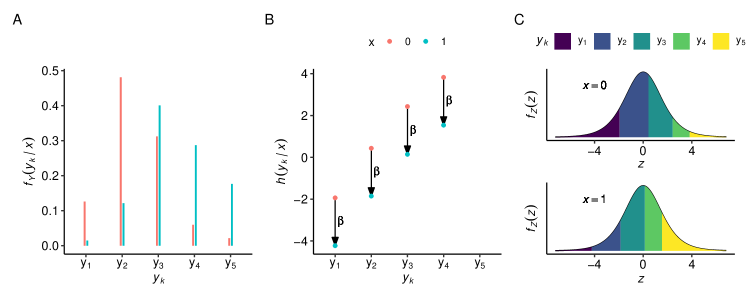
Figure 3: The conditional probability density, transformation function and latent representation of the ordinal outcome $Y$ with 5 classes depending on a single predictor $x$ which is increased by $\Delta x=1$ from 0 to 1. The density of $(Y\rvert x)$ for $x=0$ and $x=1$ is shown in A. The simple linear shift model (see eq. (8)) imposes a downward shift of the transformation function by $\beta$ when increasing the predictor from $x=0$ to $x=1$ (B). The shift in the transformation function translates into a shift in the conditional cut points $h(y_{k}\rvert\boldsymbol{x})$ under the density of the latent variable $Z$ (C). Shifting the transformation function downwards results in higher probabilities of $Y$ belonging to a higher class.

The popularity of this transformation model with $F_{Z}=F_{\operatorname{L}}$ is due to the insightful interpretation of the parameter $\beta_{j}$ as demonstrated in the following.

Based on the simple distribution $F_{Z}$ and the transformation function $h$, the odds for the outcome to belong to a class higher than class $y_{k}$ can be written as

$$\operatorname{odds}(Y>y_{k}\rvert\boldsymbol{x}) =\frac{\mathbb{P}(Y>y_{k}\rvert\boldsymbol{x})}{\mathbb{P}(Y\leq y_{k}\rvert\boldsymbol{x})}=\frac{1-F_{Y}(y_{k}\rvert\boldsymbol{x})}{F_{Y}(y_{k}\rvert\boldsymbol{x})}$$

$$=\frac{1-F_{Z}(h(y_{k}\rvert\boldsymbol{x}))}{F_{Z}(h(y_{k}\rvert\boldsymbol{x}))}=\frac{1-F_{\operatorname{L}}(\vartheta_{k}-\boldsymbol{x}^{\top}\text{\boldmath$\beta$})}{F_{\operatorname{L}}(\vartheta_{k}-\boldsymbol{x}^{\top}\text{\boldmath$\beta$})}.$$ (9)

When increasing the predictor $x_{j}$ by one unit and holding all other predictors constant we change the vector $\boldsymbol{x}$ to $\boldsymbol{x}^{\prime}$ and obtain, after some basic mathematical transformation (cf. Appendix C),

$$\operatorname{odds}(Y>y_{k}\rvert\boldsymbol{x}^{\prime}) =\frac{1-F_{\operatorname{L}}(\vartheta_{k}-\boldsymbol{x}^{\prime\top}\text{\boldmath$\beta$})}{F_{\operatorname{L}}(\vartheta_{k}-\boldsymbol{x}^{\prime\top}\text{\boldmath$\beta$})}=\frac{1-F_{\operatorname{L}}(\vartheta_{k}-\boldsymbol{x}^{\top}\text{\boldmath$\beta$}-\beta_{j})}{F_{\operatorname{L}}(\vartheta_{k}-\boldsymbol{x}^{\top}\text{\boldmath$\beta$}-\beta_{j})}$$ (10)

$$=\operatorname{odds}(Y>y_{k}\rvert\boldsymbol{x})\cdot\exp(\beta_{j}).$$

Note that the odds change by a constant factor $\exp(\beta_{j})$ independent of $k$. Hence, the parameter $\beta_{j}$ in the linear shift term can be interpreted as the log-odds ratio of the outcome belonging to a higher outcome class than $y_{k}$ when increasing the predictor $x_{j}$ by one unit and holding the remaining predictors constant with

$$\log\operatorname{OR}_{\boldsymbol{x}\to\boldsymbol{x}^{\prime}}=\log\left(\frac{\operatorname{odds}(Y>y_{k}\rvert\boldsymbol{x}^{\prime})}{\operatorname{odds}(Y>y_{k}\rvert\boldsymbol{x})}\right)=\beta_{j}.$$ (11)

This is depicted in Figure 3 for a positive valued $\beta$, where the effect of increasing the corresponding feature by one unit increases the odds for the outcome to belong to a higher class. More specific, the odds of the outcome for a higher class than $y_{k}$ is increased by a factor $\exp(\beta_{j})$, which holds for each $y_{k}$. Because the effect of $\beta$ is the same for each class boundary these models are referred to as proportional odds models (Tutz, 2011).

2.3 Related Work

Prediction models for ordinal outcomes have been studied in machine learning as extensions of different popular methods like Gaussian Processes (Chu and Ghahramani, 2005), support vector machines (Chu and Keerthi, 2007), and neural networks (Cardoso and Costa, 2007). With the advent of deep learning, various approaches have been proposed to tackle classification and regression tasks with ordinal outcomes, which we describe in more detail in the following. Note that we refer to models, which aim to predict a valid entire conditional outcome distribution as ordinal regression models, whereas models, which focus on the predicted class label will be referred to as ordinal classification models. For instance, the MCC model described in Section 2 is a regression model (i.e. multinomial regression), whereas most of the state-of-the-art approaches described below are ordinal classifiers. In the following we discuss literature on ordinal classification and literature related to different aspects of our work, i.e. regression models, transformation models, and interpretability.

Ordinal classification

Deep learning approaches to ordinal regression and classification problems range from using an ordinal metric for the evaluation of multi-class classification models to the construction of novel ordinal loss functions and dummy encodings. The earliest approaches made use of the equivalence of an ordinal prediction problem with outcome $Y\in\{y_{1}<\dots<y_{K}\}$, to the $K-1$ binary classification problems given by $\mathbbm{1}(Y\leq y_{k})$, $k=1,\dots,K$ (Frank and Hall, 2001), which is still being used in applications such as age estimation (Niu et al., 2016).

Cheng et al. (2008) devised a cumulative dummy encoding for the ordinal response where for $Y=y_{k}$ we have $y_{i}=1$ if $i\leq k$ and 0 otherwise. Cheng et al. then suggest a sigmoid activation for the last layer of dimension $K$, together with two loss functions (relative entropy and a squared error loss). Similar approaches remain highly popular in application. For instance, Cao et al. (2019) extend the approach to rank-consistent ordinal predictions. The problem of rank inconsistency, however, is confined to the $K$-rank and similar approaches and does not appear in ordinal regression models, such as the ones we propose.

Xie and Pun (2020) used a similar dummy encoding to train $K-1$ binary classifiers, which share a common CNN trunk for image feature extraction but possess their own fully connected part. This allows flexible feature extraction while reducing model complexity substantially due to weight sharing. Weight sharing is a natural advantage of models which are trained with an ordinal loss function instead of multiple binary losses, which we describe next. A comparison of ontram against the method described in Xie and Pun (2020) can be found in Appendix F.

Recently, the focus shifted towards novel ordinal loss functions involving Cohen’s kappa, which was first proposed by (de La Torre et al., 2018) and subsequently used in “proportional odds model (POM) neural networks” (Vargas et al., 2019). POM neural networks and their extensions to other cumulative link functions in (Vargas et al., 2020) are closely related to ontrams, proposed in this paper, because they constitute a special case in which the class-specific intercepts do not depend on input data (see Section 3). The crucial difference between POM NNs (as proposed in (Vargas et al., 2019)) and ontrams is the quadratic weighted Cohen’s kappa (QWK) loss function in POM NNs, compared to a log-likelihood loss in ontrams. Although POM NNs predict a full conditional outcome distribution, their focus lies on optimizing a classification metric (QWK). The idea is to penalize misclassifications that are further away from the observed class stronger than misclassifications that are closer to the observed class. In contrast, in regression approaches, the goal is to predict a valid probability distribution across all classes. We give more detail on and compare our proposed method against the QWK loss in Appendices D and F, respectively. We use QWK-based models as an example to address the general problem arising when comparing classification and regression models, which address different questions and hence optimize distinct target functions.

Ordinal regression

Lastly, Liu et al. (2019) took a probabilistic approach using Gaussian processes with an ordinal likelihood similar to the cumulative probit model (cumulative ordinal model with $F_{Z}=\Phi$) and a model formulation similar to POM neural networks. We address further related work concerning technical details in Section 3, such as the explicit formulation of constraints in the loss function.

Transformation models

Deep conditional transformation models have very recently been applied to regression problems with a continuous outcome (Sick et al., 2021; Baumann et al., 2020). Both approaches, as well as our contribution, can be seen as special cases of semi-structured deep distributional regression, which was proposed by Rügamer et al. (2020). Sick et al. parametrized the transformation function as a composition of linear and sigmoid transformations and a flexible basis expansion that ensures monotonicity of the resulting transformation function. The authors applied deep transformation models to a multitude of benchmark data sets with a continuous outcome and demonstrated a performance that was comparable to or better than other state-of-the-art models. However, in one of the benchmark data set the authors treated a truly ordinal outcome as continuous, as done by all the other benchmark models. This is indicative for the lack of deep learning models for ordered categorical regression.

Interpretability

In general, deep learning models suffer from a lack of interpretability of the predictions they make (Goodfellow et al., 2016). In DL models related to image data, interpretability is mostly referred to as highlighting parts of the image that explain the respective prediction. Often, surrogate models are build on top of the black-box model’s predictions, which are easier to interpret. One such model is LIME (Ribeiro et al., 2016). For problems with an ordinal outcome, Amorim et al. (2018) comment on the limited interpretability of the ensemble of neural networks in the $K$-rank approach described above and propose to use a mimic learning technique, which combines the ensemble with a more directly interpretable model. In the present work we take a different approach to interpretability rooted in statistical regression models. The interpretability of the effect of individual input features is given by the fitted model parameters in an additive transformation function, which is a common modelling choice for achieving interpretability (Rudin, 2019). Agarwal et al. (2020) take the same approach in the framework of generalized additive models (GAMs). We give more detail in Section 2.2.2 and Appendix C.

3 Ordinal Neural Network Transformation Models

Here, we present ordinal neural network transformation models, which unite cumulative ordinal regression models with deep neural networks and seamlessly integrate complex data like images ($\mathsf{B}$) and/or tabular data ($\boldsymbol{x}$). At the heart of an ontram lies a parametric transformation function $h(y_{k}\rvert\boldsymbol{x},\mathsf{B})$, which transforms the ordinal outcome $y_{k}$ to cut points of a continuous latent variable and controls the interpretability and flexibility of the model (see Figure 2). The ordering of the outcome is incorporated in the ontram loss function by defining it via the cumulative distribution function

$$\text{NLL}:=-\frac{1}{n}\sum_{i=1}^{n}\log\left(F_{Z}(h(y_{ki}\rvert\boldsymbol{x}_{i},\mathsf{B}_{i}))-F_{Z}(h(y_{(k-1)i}\rvert\boldsymbol{x}_{i},\mathsf{B}_{i}))\right).$$ (12)

In the following we describe the terms of the parametric transformation function and their interpretability. The parameters of these terms are controlled by NNs, which are jointly fitted in an end-to-end fashion by minimizing the NLL (Figure 4).

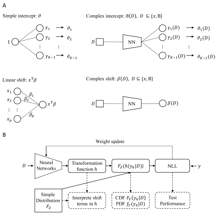
Figure 4: Architecture building blocks of ontrams. A: Simple intercept and linear shift terms are modeled using a single-layer neural network. Complex intercept and complex shift terms are allowed to depend on the input data in a more complex manner and may be a fully connected or convolutional NN depending on the type of the input data. The input data $D$ can be a single tabular predictor $x_{j}$ or a set of tabular predictors $\boldsymbol{x}$ or images $\mathsf{B}$. B: The output of the NNs control the additive components of the transformation function $h$. Together with the choice of $F_{Z}$, $h$ determines the full model, from which the likelihood can be evaluated. During training time (solid lines) the weights of all model components are trained jointly by minimizing the NLL. After training (dashed lines) the shift terms in the transformation function can be interpreted, the conditional outcome distribution can be predicted and the NLL can be evaluated for a given test set.

Modularity

The transformation function, which determines the complexity and interpretability of an ontram, consists of an intercept term, optionally followed by additive shift terms, which depend in a more or less complex manner on different input data and are controlled by NNs (see Figure 4).

The intercept term controls the shape of the transformation function:

1. Simple intercepts (SI) $\vartheta_{k}$, $k=1,\dots,K-1$ are unconditional, i.e. the shape of the transformation function is independent of the input data. SIs can be modeled as a single layer neural network with $K-1$ output units and linear activation function. The input is given by 1. The outputs are given by $\gamma_{1},\dots,\gamma_{K-1}$ controlling the intercepts (see Figure 4).

2. Complex intercepts (CI), on the other hand, depend on the input data, which may be tabular data, image data or a combination of both, yielding $\vartheta_{k}(\boldsymbol{x})$, $\vartheta_{k}(\mathsf{B})$, or $\vartheta_{k}(\boldsymbol{x},\mathsf{B})$, respectively. CIs enable more complex transformation functions, whose shape may vary with the input. Depending on the type of input data, CIs are modeled using a multi-layer fully connected neural network, a convolutional neural network or a combination of both. Analogous to SI terms, the number of output units in the last layer is equal to $K-1$ with linear activation function, yielding $\gamma_{1}(\boldsymbol{x},\mathsf{B}),\dots,\gamma_{K-1}(\boldsymbol{x},\mathsf{B})$ depending on the input (see upper right panel in Figure 4).

To ensure that the transformation function is non-decreasing, the outputs $\gamma_{1},\dots,\gamma_{K-1}$ of simple and complex intercept models are transformed before entering the likelihood via

$$\begin{split}\vartheta_{k}&=\vartheta_{1}+\sum_{i=2}^{k}\exp(\gamma_{i}),\quad k=2,\dots,K-1,\\ \vartheta_{0}&=-\infty,\;\vartheta_{1}=\gamma_{1},\;\vartheta_{K}=+\infty.\end{split}$$ (13)

The addition of $\vartheta_{0}=-\infty$ and $\vartheta_{K}=+\infty$ is important for computing the loss as described in Section 2. Enforcing a monotone increasing transformation function via eq. (13), such that $\vartheta_{0}<\vartheta_{1}\leq\dots<\vartheta_{K}$, has been done similarly in the literature. In what Cheng et al. (2008) call threshold models, $\gamma_{i}$ is squared instead of taking the exponential to ensure the intercept function is non-decreasing (Liu et al., 2019; Vargas et al., 2020). A different but related approach is to softly penalize the loss for pair-wise rank inconsistencies using a hinge loss (Liu et al., 2017b, 2018). Note that the special case $\vartheta_{k}(\boldsymbol{x},\mathsf{B})$ already includes both tabular and image data. That is, the transformation function and therefore the outcome distribution is allowed to change with each input $\boldsymbol{x}$ and $\mathsf{B}$, which represents the most flexible model possible. In fact, this most flexible ontram is equivalent to a MCC model with softmax as last-layer activation function and a categorical cross-entropy loss, albeit parametrized differently to take the order of the outcome into account.

Shift terms impose data dependent vertical shifts on the transformation function:

1. Linear shift (LS) terms $\boldsymbol{x}^{\top}\text{\boldmath$\beta$}$ are used for tabular features and are directly interpretable (see Section 2.2.2). The components of the parameter $\beta$ can be modeled as the weights of a single layer neural network with input $\boldsymbol{x}$, one output unit with linear activation function and without a bias term (see lower left panel in Figure 4).

2. Complex shift (CS) terms depend on tabular predictors or image data. Complex shift terms are modeled using flexible dense and/or convolutional NNs with input $\boldsymbol{x}$ and/or $\mathsf{B}$, and a single output unit with linear activation (see lower right panel in Figure 4). Similar to linear shift terms, the output of $\beta$ and $\eta$ can be interpreted as the log odds of belonging to a higher class, compared to all lower classes, if $F_{Z}=F_{\operatorname{L}}$. Again, this effect is common to all class boundaries. In contrast to a linear shift term, we can model a complex shift for each tabular predictor $\beta(x_{j})$ akin to a generalized additive model. Alternatively, we can model a single complex shift $\beta(\boldsymbol{x})$ for all predictors, which allows for higher order interactions between the predictors. This way, the interpretation of an effect of a single predictor is lost in favour of higher model complexity.

Interpretability and flexibility

In the following, we will present a non-exhaustive collection of ontrams integrating both tabular and image data. We start to introduce the least complex model with the highest degree of interpretability and end with the most complex model with the lowest degree of interpretability.

The simplest ontram conditioning on tabular data $\boldsymbol{x}$ and image data $\mathsf{B}$ is given by

$$h(y_{k}\rvert\boldsymbol{x},\mathsf{B})=\vartheta_{k}-\boldsymbol{x}^{\top}\text{\boldmath$\beta$}-\eta(\mathsf{B}),$$ (14)

where $\vartheta_{k}$ is a simple intercept corresponding to class $k$, $\beta$ is the weight vector of a single layer NN as described above and $\eta(\mathsf{B})$ the output of a CNN (Figure 4 A). In this case, $\beta$ and $\eta$ can be interpreted as cumulative log odds-ratios when choosing $F_{Z}=F_{\operatorname{L}}$ (see Section 2.2.2). The above model can be made more flexible, yet less interpretable, by substituting the linear predictor for a more complex neural network $\beta$, such that

$$h(y_{k}\rvert\boldsymbol{x},\mathsf{B})=\vartheta_{k}-\beta(\boldsymbol{x})-\eta(\mathsf{B}),$$ (15)

where $\beta(\boldsymbol{x})$ is now a log odds ratio function that allows for higher order interactions between all predictors in $\boldsymbol{x}$. For instance, one may be interested in the odds ratio $\operatorname{OR}_{\mathsf{B}\to\mathsf{B}^{\prime}}$ of belonging to a higher category when changing an image $\mathsf{B}$ to $\mathsf{B}^{\prime}$ and holding all other variables constant. As a special case, complex shifts include an additive model formulation in the spirit of generalized additive models (GAMs) by explicitly parametrizing the effect of each predictor $x_{j}$ with a single neural network $\beta_{j}$ (Agarwal et al., 2020)

$$h(y_{k}\rvert\boldsymbol{x},\mathsf{B})=\vartheta_{k}-\sum_{j=1}^{J}\beta_{j}(x_{j})-\eta(\mathsf{B}),\;j=1,\dots,J.$$ (16)

For $F_{Z}=F_{\operatorname{L}}$ the complex shift term $\beta_{j}(x)$ can be interpreted as a log-odds ratio for the outcome to belong to a higher class than $y_{k}$ compared to the scenario where $\beta_{j}(x)=0$, all other predictors kept constant.

Another layer of complexity can be added by allowing the intercept function $\vartheta_{k}$ for $Y=y_{k}$, to depend on the image

$$h(y_{k}\rvert\boldsymbol{x},\mathsf{B})=\vartheta_{k}(\mathsf{B})-\beta(\boldsymbol{x}).$$ (17)

In this transformation function we call $\vartheta_{k}(\mathsf{B})$ complex intercept, because the intercept function is allowed to change with the image (Figure 4 A). One does not necessarily have to stop here. Including both the image and the tabular data in a complex intercept

$$h(y_{k}\rvert\boldsymbol{x},\mathsf{B})=\vartheta_{k}(\boldsymbol{x},\mathsf{B})$$ (18)

represents the most flexible model whose likelihood is equivalent to the one used in MCC models, solely with a different parametrization. Consequently, solely the most flexible ontrams achieve on-par performance compared with deep classifiers trained using the cross-entropy loss, while the less flexible ontrams are attractive because of their easier interpretability. In fact, we illustrate empirically that a minor trade-off in predictive performance leads to a considerable ease in interpretation.

Computational details

The parameters of an ontram are jointly trained via stochastic gradient descent. The parameters enter the loss function via the outputs of the simple/complex intercept and shift terms modeled as neural networks (see Figure 4 A). The gradient of the loss with respect to all trainable parameters is computed via automatic differentiation in the TensorFlow framework. Note that any pre-implemented optimizer can be used and that there are no constraints on the architecture of the individual components besides their last-layer dimension and activation function.

4 Experiments

We perform several experiments on data with an ordinal outcome to evaluate and benchmark ontrams in terms of prediction performance and interpretability. For the experiments we use two publicly available data sets as presented in the following section. In addition, we simulate tabular predictors to assess estimation performance for the effect estimates in ontrams.

4.1 Data

UTKFace

UTKFace contains more than 23000 images of faces belonging to all age groups (dataset Song and Zhang, Accessed: April 2020). The ordinal outcome is determined by age using the classes baby (0–3, $n_{0}=1894$), child (4–12, $n_{1}=1519$), teenager (13–19, $n_{2}=1180$), young adult (20–30 $n_{3}=8068$), adult (31–45, $n_{4}=5433$), middle aged (46–61, $n_{5}=3216$) and senior ($>$61, $n_{6}=2395$) (dataset Das et al., 2018). The images are labeled with the people’s age (0 to 116) from which the age-class is determined. In addition, the data set provides the tabular feature sex (female, male). As our main goal is not on performance improvement but on the evaluation of our proposed method, we use the already aligned and cropped versions of the images. For some example images see Figure 5.

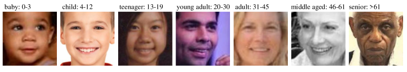
Figure 5: Example images for UTKFace. Example images of the seven ordinal age-classes (baby, child, teenager, young adult, adult, middle aged and senior) of the cropped and aligned UTKFace data set are presented.

We simulate tabular predictors $\boldsymbol{x}$ with predefined effects on the ordinal outcome of the UTKFace data set, where we assume a proportional odds model $F_{Y}(y_{k}\rvert\boldsymbol{x})=F_{Z}(\vartheta_{k}-\boldsymbol{x}^{\top}\text{\boldmath$\beta$})$ (see Section 2.2.2). The simulation scheme is closely related to choice-based sampling (Manski and Lerman, 1977). Ten predictors are simulated, four of which are noise predictors that have no effect on the outcome. The six informative predictors are simulated to have an effect of $\pm\log 1.5$, $\pm\log 2$ and $\pm\log 3$ on the log-odds scale, to reflect small to large effect sizes commonly seen in medical and epidemiological applications. All predictors are mutually independent of each other and the image data. The predictors are simulated from the conditional distribution $X_{j}\rvert\boldsymbol{y}\sim\mathcal{N}(\boldsymbol{y}^{\top}\boldsymbol{\xi}_{j},\sigma^{2})$, where $\boldsymbol{y}$ denotes the one-hot encoded outcome and $(\boldsymbol{\xi}_{j})_{k}=k\cdot\beta_{j}$ for $k=1,\dots,K$, to emulate the proportional odds property. All simulated predictors have a common variance of $\sigma^{2}=1.55^{2}$, which was tuned such that the estimated $\hat{\beta}_{j}$ on average recovers the true $\beta_{j}$ when estimating the conditional distribution $Y\rvert\boldsymbol{x}$ in a proportional odds model. A summary of the simulation procedure is given in Figure 6.

Figure 6: Simulation of predictors for UTKFace data. $X_{j}\stackrel{{\scriptstyle\operatorname{i.i.d.}}}{{\sim}}\operatorname{N}(0,\sigma^{2})$, $j=1,\dots,10$, with $\sigma^{2}=1.55^{2}$. The predictors $X_{j}$ are simulated such that their effects adhere to the proportional odds assumption. That is, the effect of $\beta$ is common to all class boundaries. Note that the arrows indicate effects on the log-odds scale of the outcome $Y$, i.e., $F_{Y}(y_{k}\rvert\boldsymbol{x})=F_{L}(\vartheta_{k}-\boldsymbol{x}^{\top}\text{\boldmath$\beta$})$. The dotted arrow from $\mathsf{B}$ to $Y$ indicates that the image is not entering the simulation directly but is assumed to have an effect on the outcome.

Wine quality

The Wine quality data set consists of 4898 observations (dataset Cortez et al., 2009). The ordinal outcome describes the wine quality measured on a scale with 10 levels of which only 6 consecutive classes (3 to 8, $n_{3}=10$, $n_{4}=53$, $n_{5}=681$, $n_{6}=638$, $n_{7}=199$, $n_{8}=18$) are observed. The data set contains 11 predictors, such as acidity, citric acid and sugar content. As in Gal and Ghahramani (2016), we consider a subset of the data (red wine, $n=1599$).

4.2 Models

The models we use for evaluating and benchmarking the proposed ontrams are summarized in Table 2.

Table 2: Summary of the models used for evaluating the ontram methods. In the upper part we list models used for the Wine data, which contain only tabular predictors ($\boldsymbol{x}$). In the lower part, we show models for the UTKFace data, which consist of image data and tabular predictors $(\boldsymbol{x},\mathsf{B})$. Above the thin lines we list the baseline models; below the ontrams. For each model, which can be framed as a transformation model, the transformation function is given. Parameters in the shift terms of a transformation function can be interpreted as log odds-ratios if $F_{Z}$ is chosen to be the standard-logistic distribution. Then, any model involving a simple intercept is an instance of a proportional odds model.

Data set	Model name	Abbreviation	Trafo $h(y_{k}\rvert\boldsymbol{x},\mathsf{B})$
UTKFace	Multi-class classification	MCC
	Multi-class classification + tabular	MCC-$\boldsymbol{x}$
	Complex intercept	CIB	$\vartheta_{k}(\mathsf{B})$
	Complex intercept + tabular	CIB-LSx	$\vartheta_{k}(\mathsf{B})-\boldsymbol{x}^{\top}\text{\boldmath$\beta$}$
	Simple intercept + complex shift	SI-CSB	$\vartheta_{k}-\eta(\mathsf{B})$
	Simple intercept + complex shift + tabular	SI-CSB-LSx	$\vartheta_{k}-\eta(\mathsf{B})-\boldsymbol{x}^{\top}\text{\boldmath$\beta$}$
	Simple intercept + tabular	SI-LSx	$\vartheta_{k}-\boldsymbol{x}^{\top}\text{\boldmath$\beta$}$
Wine	Multi-class classification	MCC
	Generalized additive proportional odds model	GAM	$\vartheta_{k}-\sum_{j=1}^{p}\beta_{j}(x_{j})$
	Proportional odds logistic regression	polr	$\vartheta_{k}-\boldsymbol{x}^{\top}\text{\boldmath$\beta$}$
	Complex intercept	CIx	$\vartheta_{k}(\boldsymbol{x})$
	Simple intercept + GAM complex shift	SI-CS${}^{\star}_{\boldsymbol{x}}$	$\vartheta_{k}-\sum_{j=1}^{p}\beta_{j}(x_{j})$
	Simple intercept + linear shift	SI-LSx	$\vartheta_{k}-\boldsymbol{x}^{\top}\text{\boldmath$\beta$}$

These models feature a different flexibility and interpretability and are trained with the different loss functions described in Sections 2 and 3.

4.3 Training and Validation Setup

The models are implemented and evaluated on the UTKFace and Wine quality data set as described in the following. The NN architectures used for the different applications are summarized in Appendix A.

UTKFace

The UTKFace data set is split into a training (80%) and a test set (20%); 20% of the training set is used as validation data. The images are resized to $128\times 128\times 3$ pixels. The resized images are normalized to have pixel values between 0 and 1. No further preprocessing is performed. The models are trained for up to 100 epochs with the Adam optimizer with a batch size of 32 and a learning rate of 0.001. Overfitting is addressed with early stopping. That is, we retrospectively search for the epoch in which the validation loss is minimal and consider the respective parameters for our trained models.

We analyse the data set using deep ensembling (Lakshminarayanan et al., 2017), a state of the art approach in probabilistic deep learning methods leading to more reliable probabilistic predictions (Wilson and Izmailov, 2020). Specifically, models are trained five times with a different weight initialization in each iteration. The resulting predicted conditional outcome distribution is averaged over the five runs and this averaged conditional outcome distribution is then used for model evaluation. This procedure is supposed to prevent double descent and improve test performance (Wilson and Izmailov, 2020).

Wine quality

For analyses of the wine quality data we employ the same cross-validation scheme as Gal and Ghahramani (2016) and split the data into 20 folds of 90% training and 10% test data. The predictors are normalized to the unit interval. Otherwise, no further preprocessing is performed. The architectures of the used NNs are described in Appendix A. All NNs are jointly trained via stochastic gradient descent using a learning rate of 0.001. The linear shift model is trained for 8000 epochs with a batch size of 90. The ontram GAM is trained for 1200 epochs with a batch size of 180. All other models are trained for 100 epochs with a batch size of 6.

4.4 Software

We implement MCC models and ontrams in the two programming languages R 3.6-3 and Python 3.7. The models are written in Keras based on a TensorFlow backend using TensorFlow version $>$2.0 (Chollet et al., 2015; Abadi et al., 2015) and trained on a GPU. Both polr and generalized additive proportional odds models are fitted in R using tram::polr() (Hothorn, 2020) and mgcv::gam() (Wood, 2017), respectively. Further analysis and visualization is performed in R. For reproducibility, all code is made available on GitHub.

4.5 Model Evaluation

Evaluation metrics: The main focus of ontrams is to be able to interpret their individual components and the most flexible ontram is equivalent to the MCC model. In turn, prediction performance of ontrams can only ever be as good as in MCC. Therefore, we assess prediction performance mainly to illustrate trading off model flexibility against ease of interpretation. We evaluate the prediction performance of ontrams and MCCs with proper scoring rules, namely the negative log-likelihood (NLL) and the ranked probability score (RPS). Roughly speaking, proper scoring rules encourage honest probabilistic predictions because they take their optimal value when the predicted conditional outcome distribution corresponds to the data generating distribution (for details see Appendix E). In Appendix G we compute additional evaluation metrics which are commonly used for ordinal classification models, i.e. accuracy and QWK which is discussed in Appendix D.

Estimation and interpretability

To evaluate whether ontrams yield reliably interpretable effect estimates of shift components we make use of the simulated tabular predictors and compare the known true effects of the individual predictors to the estimates. For other predictors we discuss the plausibility of the estimated effects or, if applicable, compare them to results of other benchmark experiments.

5 Results

Results for the MCC models and ontrams for the UTKFace and wine data are given in the following Sections 5.1 and 5.2, respectively.

5.1 UTKFace

We first evaluate ontrams on the UTKFace data set, which contains images and tabular predictors that allow to illustrate the interpretation of the shift terms. As in other applications, age is discretized and treated as an ordinal outcome (see e.g. (Liu et al., 2017a)).

We first train a SI-CS_B-LS${}_{\text{sex}}$ ontram with transformation function $h(y_{k}\rvert\boldsymbol{x})=\vartheta_{k}-\eta(\mathsf{B})-\beta_{\text{sex}}\cdot\mathds{1}(\text{sex}=\text{female})$ that includes the tabular predictor sex in addition to the images. We assume that the prediction of the age class depends on the appearance of a person and therefore on the image but not on a person’s sex. On the other hand, a person’s sex can often be deduced from an image, which renders the tabular feature and image data collinear and makes estimation and interpretability of the individual effects more difficult. However, collinear data is representative for most practical applications. We thus expect the estimated coefficient $\beta_{\text{sex}}$ to be small in comparison to the effect of the image $\eta(\mathsf{B})$, which we expect to be a better predictor of a person’s age.

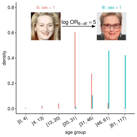
Figure 7: Predicted densities in a SI-CS_B-LS${}_{\text{sex}}$ ontram once using the image of a 41 year-old and a 67 year-old Meryl Streep, while the gender is female in both cases. What sets ontrams apart from other ordinal DL classifiers, is the directly interpretable effect of changing an image in terms of a log odds-ratio. Namely, the odds of belonging to a higher age change by a factor of $\exp(5)$ when changing image $\mathsf{B}$ to $\mathsf{B}^{\prime}$, keeping sex constant. In turn, a change in the odds results in a change of the corresponding conditional outcome distribution, which puts higher probability mass on larger age groups when changing $\mathsf{B}$ to $\mathsf{B}^{\prime}$.

For evaluation, we use publicly available data of the actress Meryl Streep, i.e., female sex and two images showing her at the age of 41 ($\mathsf{B}$, age group $[31,46)$) and 67 ($\mathsf{B}^{\prime}$, age group $[61,117)$) to depict the predicted PDF and estimated log odds-ratio in the SI-CS_B-LS${}_{\text{sex}}$ model (see Figure 7). The model yields the image-effect estimates $\eta(\mathsf{B})=5.1$ and $\eta(\mathsf{B}^{\prime})=10.1$, while the effect of sex stays constant ($\beta_{\text{sex}}=0.3$). As expected $\eta(\mathsf{B}^{\prime})>\eta(\mathsf{B})$, indicating that $\mathsf{B}^{\prime}$ is more likely to belong to a higher age group than $\mathsf{B}$. In particular, the difference between the two estimates yields a log odds-ratio $\eta(\mathsf{B}^{\prime})-\eta(\mathsf{B})=5$, which is interpretable as an $\exp(5)$-fold increase in the odds of belonging to a higher age class compared to all classes below, when changing from $\mathsf{B}$ to $\mathsf{B}^{\prime}$ and keeping sex constant.

For a more systematic and empirical evaluation of the flexibility and interpretability of ontrams, we fit seven models with the image data, the 10 simulated tabular predictors with known true effect sizes $\beta$ and a combination of both (see Table 2). The models differ in their flexibility due to different transformation functions and the parametrization of the loss. In Appendix F, we compare the MCC model and the CI_x ontram to another ordinal classification model trained with a loss based on Cohen’s quadratic weighted kappa (QWK, de La Torre et al., 2018).

We first consider the most flexible models, MCC and CI_B, which are based on the UTKFace image data and only differ in the parametrization of the loss function (see eq. 2 for the MCC and eq. 12 for the ontram loss). As expected, the CI_B ontram and MCC model achieve comparable prediction performances in terms of NLL and RPS (see Figure 8 A and B). After including the simulated tabular predictors, the performance in both models increases notably (see MCC-$\boldsymbol{x}$ and CI_B-LS_x in Figure 8 A and B). In case of the MCC-$\boldsymbol{x}$ model, the tabular predictors are attached to the feature vector resulting from the convolutional part of the CNN, which allows interactions between image and tabular predictors and therefore makes the model slightly more flexible than the CI_B-LS_x. However, in contrast to the CI_B-LS_x, the MCC-$\boldsymbol{x}$ allows no interpretation of the effect of the tabular predictors on the outcome.

Less flexible but more interpretable ontrams are obtained by including the image data as complex shift rather than as complex intercept term (SI-CS_B). Although the SI-CS_B model is less flexible than the CI_B model, prediction performance is comparable (see Figure 8 A and B). Again, adding the simulated tabular data as a linear shift term (SI-CS_B-LS_x) results in improved prediction performance.

Using a model with simulated tabular data only (SI-LS_x) yields a better performance than models that include image data only (see SI-LS_x vs. MCC, CI_B, SI-CS_B in Figure 8 A and B). However, when comparing the models with image data and tabular predictors to the model with tabular predictors only, an increase in prediction performance is observed (see SI-LS_x vs. MCC-$\boldsymbol{x}$, CI_B-LS_x and SI-CS_B-LS_x). This indicates that the images contain additional information for age prediction.

In practice, the ontrams CI_B-LS_x and SI-CS_B-LS_x are most attractive because they provide interpretatable estimates for the effects of the tabular predictors with an acceptably low decrease in prediction performance.

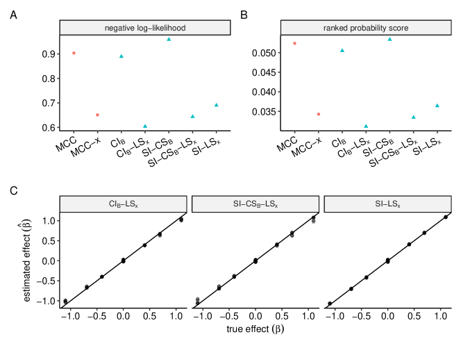
Figure 8: Test prediction performance for deep ensembles based on the UTKFace data. The figure summarizes the results for the models MCC, MCC-$\boldsymbol{x}$, CI_B, CI_B-LS_x, SI-CS_B, SI-CI_B-LS_x, SI-LS_x (x-axes) in terms of negative log-likelihood (A) and ranked probability score (B). Lower values in NLL and RPS indicate improved model performance. Baseline models are highlighted in red, ontrams in blue. C: True versus estimated predictor effects. The figure summarizes the true versus estimated effects of the simulated tabular predictors of the UTKFace data set. The effect estimates result from the linear shift terms, LS_x, in the models CI_B-LS_x, SI-CS_B-LS_x, SI-LS_x. In case of correct estimation, the parameters lie on the main diagonal.

To assess whether effect estimates for the tabular predictors are reliable in models with and without additional image data, we compare the true effects $\beta$ to the estimated effects $\hat{\beta}$ for the ontrams with linear shift terms (CI_B-LS_x, SI-CS_B-LS_x, SI-LS_x). As summarized in Figure 8 C, all models recover the correct estimates.

5.2 Wine Quality

The experiments with the UTKFace data have shown that we get reliable and interpretable model components when including simulated, mutually independent tabular predictors besides image data. In the following, we summarize a couple of experiments with the smaller wine data set containing solely tabular predictors to demonstrate how we can estimate reliable linear and non-linear effect estimates for potentially dependent tabular predictors. In addition, we evaluate how the ontram parametrization of the loss (see eq. 12) yields a gain in training speed and how this gain depends on the size of the training data. Note that all those models can simply be extended to additionally include image data, e.g. by attaching a complex shift term CS_B.

The wine dataset is a benchmark data set for a proportional odds model that allows to interpret the fitted effect estimates as log odds-ratios (see Section 2.2.2). To illustrate the high flexibility of ontrams and that we correctly estimate linear, non-simulated tabular predictors, we fit a proportional odds model with linear effects via a SI-LS_x model and compare the model to the same model using the R function tram::Polr(). As expected, Figure 9 shows that both models yield the same prediction performance in terms of NLL (A) and RPS (B) and estimated predictor effects (C).

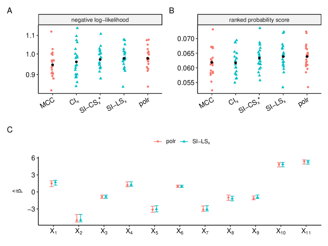
Figure 9: Results of the wine quality data based on the test sets from the cross validation setting. Panels A and B summarize the prediction performance for the models MCC, CI_x, GAM, SI-LS_x and polr (x-axes) based on the wine quality data set in terms of negative log likelihood (A) and ranked probability score (B). Lower values in NLL and RPS indicate improved model performance. Results of ontrams are indicated as blue triangles, others as red dots. The black point gives the mean across the respective metric resulting from the single CV folds. C: Effect estimates with 2.5th and 97.5th percentile for polr and SI-LS_x model over the 20 CV folds of the wine quality data set.

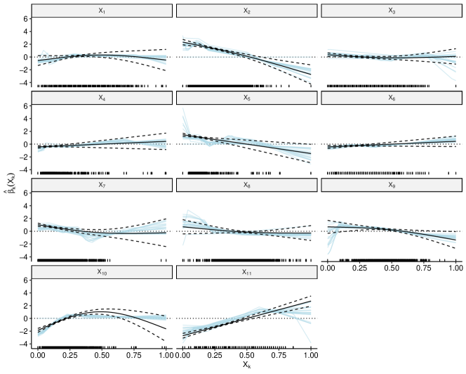
Figure 10: Estimated non-linear effects of 11 tabular predictors on the ordinal quality outcome in the wine data set as achieved by the ontram GAM model. The estimates log odds-ratio functions of an ensemble of 20 runs with different initial weights are shown in blue. The solid black line depicts the estimated log odds-ratio functions estimated by the mgcv::gam() function in R together with a 95% confidence interval (dashed black lines). Rugs on the bottom of each plot indicate the observed values for $X_{k}$, $k=1,\dots,11$, in the training data.

GAMs (see Table 2, SI-CS${}_{\boldsymbol{x}}^{*}$ with $h(y_{k}\rvert D)=\vartheta_{k}-\sum_{j=1}^{p}\beta_{j}(x_{j})$) add another layer of complexity to the model by allowing non-linear effects for each predictor. Because the individual NNs estimating the additive components $\beta_{j}(x_{J})$ do not interact explicitly the estimated log odds-ratio function retains the interpretability of a proportional odds model. Figure 10 depicts the estimates of an ensemble of ontram GAMs in comparison to a GAM from the R-package mgcv. Apart from the constraint-enforced smoothness in mgcv’s GAM, both models agree in magnitude and shape of the estimated predictor effects. For instance, predictor $X_{10}$ (sulphate content) has a strong positive influence on the rating when increased from 0 to 0.25 (on the transformed scale), in that the odds of the wine being rated higher increase by a factor of $7.4$, all other predictors held constant ($\exp(\hat{\beta}_{10}(0.25)-\hat{\beta}_{10}(0))\approx\exp(2)\approx 7.4$). Afterwards the effect levels off and stays constant for the ontram GAM, due to regularization and few wines with higher sulphate levels being present in the training data. The curve estimated by mgcv follows smoothness constraints and instead drops with a large confidence interval, also covering 0. GAMs are a special case of complex shift models, the latter of which allow for higher order interactions between the predictors. Conceptually, ontrams enable to further trade off interpretability and flexibility by modelling some predictor effects linearly while including others in a complex shift or intercept term. If field knowledge suggests non-linearity of effects or interacting predictors, they can be included as a complex shift or, if the proportionality assumption is violated, in a complex intercept term. From Figure 10 we can see that most of the coefficients could be safely modelled in a linear fashion, which is also evident from the minor loss in predictive power when comparing the GAM against the linear shift ontram (see Figure 9 A, GAM vs. SI-LS_x).

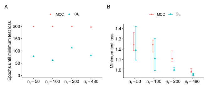
Figure 11: Epochs until minimum test loss for varying sizes of the training data using the wine quality data set. The data are split into $n/n_{t}$, $n_{t}\in\{50,100,200,480\}$ folds each of which serves as training data for a multi-class classification and a complex intercept ontram. The median test loss is computed for each scenario $n_{t}$ and each epoch. Afterwards, the number of epochs until minimum median test loss and the minimum median test loss are recorded. Here the epochs until minimum test loss (A) and the minimum test loss (B) are plotted against the 4 scenarios given by $n_{t}$.

To assess the effect of respecting the order of the ordinal outcome, we evaluate the most flexible CI_x ontram and the MCC model, which solely differ in the parametrization of their loss. As in the UTKFace data, both models show the expected agreement in achieved prediction performance w.r.t. NLL and RPS (see Figure 9 A and B). However, the CI_x model learns much faster in terms of number of epochs until the minimum test loss is achieved, compared to the MCC model. To further investigate this gain in learning speed, we split the wine quality data into $n/n_{t}$, $n_{t}\in\{50,100,200,480\}$ folds of size $n_{t}$ and fit a MCC model and CI_x ontram to each fold. The median test loss is computed for each scenario of size $n_{t}$. The number of epochs needed to achieve minimal median test loss is summarized in Figure 11 A. The training speed is consistently lower and therefore more efficient for the CI_x ontram than for the MCC model (Figure 11 A). The CI_x ontram yields a slightly better prediction performance (median test NLL) for larger sample sizes. This can be explained by the fact that after 200 epochs the MCC model still has not reached the minimum test loss (Figure 11 B). Note that the gain in training speed is only present if the outcome is truly ordered. In Appendix B, we show that the effect vanishes when the ordering of the class labels is permuted.

6 Discussion and Outlook

In this work we demonstrate how to unite the classical statistical approach to ordinal regression with DL models to achieve interpretability of selected model components. This allows us to estimate effects for the input data. In case of tabular predictors, we prove that the effects are correctly estimated, also in the presence of complex image data. Moreover, we show that the most flexible ontram trained with the reparametrized NLL achieves on-par performance with a MCC DL model using the cross-entropy loss. This may first seem counter-intuitive because the cross-entropy loss ignores the outcome’s order. However, the ontram NLL is a reparametrization of the cross-entropy loss and can, therefore, at most achieve the same performance. The advantages of reparametrizing the NLL are (i) a natural scale for the additive and hence interpretable decomposition of tabular and image effects, (ii) a valid probability distribution for the ordinal outcome and (iii) an increase in training speed. In this context, interpretability is the main advantage over other state-of-the-art models because it is of crucial importance in sensitive applications as, for example, in medicine (Rudin, 2019).

If the focus lies mainly on classification of an ordinal outcome and less on interpretability and probabilistic predictions, the data analyst may be interested in optimizing a classification metric such as Cohen’s kappa. Indeed, Cohen’s kappa directly considers the outcome’s natural order and misclassifications further away from the observed class are penalized more strongly than misclassifications closer to the observed class. However, this approach results in predictions different from those of regression models such as the MCC and CI_B, which is further highlighted in Appendix F. In a regression model, on the other hand, the goal is rather to estimate a valid probability distribution which is achieved with proper loss functions such as the NLL. These fundamental differences between ordinal classification and regression make a fair comparison nearly impossible, as we highlight in Appendix F.

Further, we demonstrate how to select an ontram, which possesses the appropriate amount of flexibility and interpretability for a given application. To achieve a higher degree of interpretability, flexibility has to be restricted, e.g. by moving from a complex intercept to a simple intercept, complex shift model. However, we show that a restriction of flexibility can still yield adequate prediction performance which may even be similar to that of a more flexible model. Interpretability of different model components is further showcased for simple models including only tabular predictors and more complex models with tabular and image data.

The modular nature of ontrams makes them highly versatile and applicable to many other problems with ordinal outcome and complex input, such as text or speech data. Instead of using a CNN for image data, a recurrent neural network can be used to define a more flexible complex intercept or a simpler, but more interpretable complex shift term as in a SI-CS_B ontram. Tabular predictors can then simply be added with linear shift or complex shift terms depending on the degree of interpretability the data analyst aims for.

This work shows the potential of deep transformation models for ordinal outcomes. The predictive power of deep transformation models on regression problems with continuous outcomes has already been demonstrated (Sick et al., 2021). However, the approach is easily extendable to the full range of existing interpretable regression models, including models for count and survival outcomes. The extension from ordinal data to count and survival data is hinted at by the parametrization of the ontram NLL, which can be viewed as an interval-censored log-likelihood over the latent variable $Z$ for which the intervals are given by the conditional cut points $h(y_{k}\rvert D)$. For count data these cut points are given by consecutive integers, i.e., $(0,1]$, $(1,2]$, and so on. In survival data the interval is given by (commonly) right censored outcomes when a patient drops out of a study or experiences a competing event. In case of right-censoring the interval is given by $(t,+\infty)$ for a patient that drops out at time $t$. All benefits in terms of interpretability and modularity will carry over to the deep transformation version of other probabilistic regression models by working with an appropriate likelihood and parametrizing the transformation function via (deep) neural networks.

Acknowledgements

We would like to thank Elvis Murina and Muriel Buri for insightful discussions and Malgorzata Roos for her feedback on the manuscript. We thank all anonymous reviewers for their comments and suggestions, which helped contextualize our proposed method among other state-of-the-art approaches. The research of LH, LK and BS was supported by Novartis Research Foundation (FreeNovation 2019). TH was supported by the Swiss National Science Foundation (SNF) under the project “A Lego System for Transformation Inference” (grant no. 200021_184603). OD was supported by the Federal Ministry of Education and Research of Germany (BMBF) in the project “DeepDoubt” (grant no. 01IS19083A).

Appendix A Neural Network Architectures

We use NNs with different architectures to explore the various additive decompositions of the transformation function described in Section 3. Simple intercept and linear shift terms are always modeled with single layer NNs without bias terms and a linear activation function (see left panel in Figure 4). For a fair comparison, we use the same NN architecture for all MCC models and for controlling the complex intercept or complex shift term in an ontram. The only difference between the models is in the output layer. MCC models feature an output layer with $K$ units and a softmax activation function. The output layer of complex intercept terms has $K-1$ output units and a linear activation function. In case of complex shift terms, the output layer consists of one unit and a linear activation function.

UTKFace

MCC, CI and CS terms are modeled with a CNN (see Figure A1). The architecture used in this work is inspired by the VGG (Simonyan and Zisserman, 2014). The convolutional part consists of three blocks while each block is comprised of two convolution and two dropout layers (with dropout rate 0.3). The blocks complete with a max-pooling layer (window size $2\times 2$ pixels, stride width 2). In the first block we use 16 filters; the following two blocks contain 32. Filter size is fixed to 3x3 pixels in every block. The fully connected part features a 500- and a 50-unit fully connected layer. The ReLU non-linearity is used as the activation function.

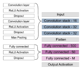
Figure A1: CNN architecture for controlling MCC models, complex intercept and complex shift terms in case of image input data. The network architecture consists of stacks of convolutional blocks consisting of multiple repetitions of a convolutional, dropout and batch-normalization layer, followed by a fully connected part.

Wine quality

MCC models, CI and CS terms are modeled using a densely connected neural network with four layers having 16 units each. Between layers 1, 2, and 3, we specify a dropout layer with dropout rate 0.3. ReLU is used as the activation function. GAMs are fitted using the same densely connected neural network for each predictor with two layers of 16 units and followed by a layer of eight units with ReLU activation. All weights were regularized using both $L_{1}$ and $L_{2}$ penalties, with $\lambda_{1}=1$ and $\lambda_{2}=5$. Between each layer there is dropout with rate 0.2.

Appendix B Learning Speed Under Permuted Class Labels

In contrast to MCC models with categorical cross-entropy loss, ontrams’ loss parametrization takes the ordering of the outcome into account (see eq. 12). This leads to more efficient learning when the outcome is truly ordered. This can be demonstrated by permuting the class label ordering of a truly ordinal outcome and inspecting the learning curves of an ontram and MCC model. When fitting the model using the true class label ordering, the ontram outperforms the MCC model in terms of learning speed and arrives at virtually the same minimum test loss (cf. Figure B1). Permuting the class label order does not affect the learning curves of the MCC model. However, the complex intercept ontram performs on-par in the presence of wrongly ordered categories in learning speed and median test loss compared to the MCC model. In general, we observe a higher variability in the loss curves between different runs when using the ontram loss parametrization.

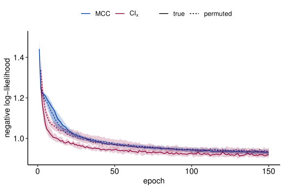
Figure B1: Test learning curves comparing a MCC against a complex intercept model (CI_x) for the true and a permuted ordering of the classes in the wine quality data set. Depicted are the median test losses (thick line) together with the empirical 20th and 80th percentile (shaded regions) over 20 runs.

Appendix C Interpretational Scales

Classical regression textbooks, like Tutz (2011), discuss $F_{Z}\in\{F_{\operatorname{L}},F_{\operatorname{MEV}},F_{\text{Gumbel}},\Phi\}$, which are called cumulative logit, minimum extreme value, maximum extreme value and probit models, respectively. Tutz (2011) also derives the interpretational scales and stresses, that the parameters resulting from a cumulative probit model are hard to interpret.

Table C1: Interpretational scales induced by $F_{Z}$ (Tutz, 2011). Same as Table 1 in the main text, restated for convenience.

$F_{Z}$	$F_{Z}^{-1}$	Symbol	Interpretation of shift terms
Logistic	$\operatorname{logit}$	$F_{\operatorname{L}}=\operatorname{expit}$	log odds-ratio
Gompertz	cloglog	$F_{\operatorname{MEV}}$	log hazard-ratio
Gumbel	loglog	$F_{\text{Gumbel}}$	log hazard-ratio for $Y_{r}=K+1-Y$
Normal	probit	$\Phi$	not interpretable directly

For $F_{Z}=F_{\operatorname{L}}:=(1+\exp(-z))^{-1}$ in a linear shift model $h(Y=y_{k}|x)=\vartheta_{k}-\boldsymbol{x}^{\top}\text{\boldmath$\beta$}$

$$\mathbb{P}(Y\leq y_{k}\rvert\boldsymbol{x}) =F_{\operatorname{L}}(\vartheta_{k}-\boldsymbol{x}^{\top}\text{\boldmath$\beta$})$$

$$\Leftrightarrow\operatorname{logit}(\mathbb{P}(Y\leq y_{k}\rvert\boldsymbol{x})) =\vartheta_{k}-\boldsymbol{x}^{\top}\text{\boldmath$\beta$}$$

$$\Leftrightarrow\log(\operatorname{odds}(Y\leq y_{k}\rvert\boldsymbol{x})) =\vartheta_{k}-\boldsymbol{x}^{\top}\text{\boldmath$\beta$}$$

$$\Leftrightarrow\log(\operatorname{odds}(Y\leq y_{k}\rvert\boldsymbol{x})) =\log(\operatorname{odds}(Y\leq y_{k}\rvert\boldsymbol{x}=0))-\boldsymbol{x}^{\top}\text{\boldmath$\beta$}$$

$$\Leftrightarrow-\log(\operatorname{odds}(Y>y_{k}\rvert\boldsymbol{x})) =-\log(\operatorname{odds}(Y>y_{k}\rvert\boldsymbol{x}=0))-\boldsymbol{x}^{\top}\text{\boldmath$\beta$}$$

$$\Leftrightarrow\operatorname{odds}(Y>y_{k}\rvert\boldsymbol{x}) =\operatorname{odds}(Y>y_{k}\rvert\boldsymbol{x}=0)\cdot\exp(\boldsymbol{x}^{\top}\text{\boldmath$\beta$}),$$

which shows that the components of $\beta$ are interpretable as log odds-ratios. In the same way, $\eta(\mathsf{B})$ in a complex shift model can be interpreted as a log odds-ratio function. Table C1 summarizes the four most commonly used cumulative ordinal regression models and the interpretational scales that different $F_{Z}$ induce.

For $F_{Z}=F_{\operatorname{MEV}}=1-\exp(-\exp(z))$ we can interpret the components of $\beta$ as log hazard ratios

$$1-F_{Y}(y\rvert\boldsymbol{x}) =\exp(-\exp(h(y)+\boldsymbol{x}^{\top}\text{\boldmath$\beta$}))=\exp(-\exp(h(y))\exp(\boldsymbol{x}^{\top}\text{\boldmath$\beta$}))$$

$$=\exp(-\exp(h(y)))^{\exp(\boldsymbol{x}^{\top}\text{\boldmath$\beta$})}=(1-F_{Y}(y\rvert\boldsymbol{x}=0))^{\exp(\boldsymbol{x}^{\top}\text{\boldmath$\beta$})}.$$

This interpretational scale is commonly used in survival analysis, Here, a log hazard ratio $\beta$ for a shift from $0$ to $\boldsymbol{x}$ is defined in terms of the conditional survivor function $S_{Y}(y\rvert\boldsymbol{x})=1-F_{Y}(y\rvert\boldsymbol{x})$ given by $S_{Y}(y\rvert\boldsymbol{x})=S_{Y}(y\rvert\boldsymbol{x}=0)^{\exp(\boldsymbol{x}^{\top}\text{\boldmath$\beta$})}$.

Appendix D Ordinal Classification With Cohen’s Kappa

Recently, DL models for ordinal classification were introduced using a transformed continuous version of the quadratic weighted kappa (QWK) as the loss function (de La Torre et al., 2018). Cohen’s kappa is usually used to assesses inter-rater agreement and corrects it for the expected number of agreements under independence

$$\kappa=\frac{p_{\text{obs}}-p_{\text{exp}}}{1-p_{\text{exp}}},$$ (19)

where $p_{\text{obs}}$ and $p_{\text{exp}}$ are the observed and expected proportion of agreement under independence. They are computed from a confusion matrix, after dividing all entries by the number of predicted instances, $p_{\text{obs}}$ is given by the sum of the diagonal elements and $p_{\text{exp}}$ by the diagonal sum of the product of the row and column marginals. An additional weighting scheme enables to penalize misclassifications far away from the observed class more strictly (Cohen, 1968) than misclassifications close to the observed class

$$\kappa_{w}=\frac{\sum_{i,j}w_{ij}o_{ij}-\sum_{i,j}w_{ij}e_{ij}}{1-\sum_{i,j}w_{ij}e_{ij}},$$ (20)

where $e$ denotes the expected and $o$ the observed number of agreements in row $i$ and column $j$ of a confusion matrix. The weights $w_{ij}=\frac{\lvert i-j\rvert^{q}}{(K-1)^{p}}$ and the exponent $q$ control the amount of penalization for predictions farther away from the observed class. Because Cohen’s kappa considers the ordinal nature of the outcome when weighted accordingly, it has been proposed and used as a loss function for deep ordinal classification problems (de La Torre et al., 2018, 2020; Vargas et al., 2019, 2020). The QWK loss is defined as

$$\ell(p)=\log(1-\kappa(p)),$$ (21)

where $p$ is the predicted probability distribution and denotes the quadratically ($q=2$) weighted Cohen’s kappa. Originally defined for count data, de La Torre et al. (2018) generalized Cohen’s kappa to be computable from a probability density and so be used as a loss function for MCC networks (when using softmax in the last layer). However, the QWK loss is an improper scoring rule and thus does not yield calibrated probabilistic predictions (cf. Appendix E). As such, we demonstrate its limited use in estimating conditional distributions for ordinal outcomes in Appendix F. However, if one were solely interested in ordinal classification, the QWK loss is useful to penalize misclassifications farther away from the observed class, where the weighting scheme controls the amount of penalization. Ordinal regression and classification are contrasted in more detail in Appendix F.

To contrast ordinal regression models with pure classification models we additionally use evaluation metrics for ordinal classifiers, such as the accuracy, continuous QWK (the QWK loss transformed back to its original scale via $1-\exp(\ell(p))$, see eq. (21)), and discrete QWK (see eq. (20)). Neither accuracy nor the QWK metrics are proper scoring rules and both can lead to misleading results when evaluating probabilistic models (cf. Appendices E and F).

Appendix E Scoring rules

Here we give a brief overview on scoring probabilistic predictions. In the end we show that the QWK loss is an improper scoring rule.

Scoring rules are used to judge the prediction quality of a probabilistic model and have their roots in information theory and weather forecasting (Gneiting and Raftery, 2005). On average, a strictly proper scoring rule only takes its optimal value if the predicted probability distribution corresponds to the “data generating” probability distribution. Assume that $p$ is the data generating probability density, then a proper score $S$ fulfills for any probability density $q$

$$\mathbb{E}_{Y\sim p}[S(p;Y)]\leq\mathbb{E}_{Y\sim p}[S(q;Y)].$$ (22)

A score is strictly proper when equality in the above holds iff $q=p$ (Gneiting and Raftery, 2007).

Bröcker and Smith (2007) stress the importance of proper scoring rules for honest distributional forecasts. The NLL is is a strictly proper scoring rule, which is why we use it in the present work. Strict propriety of the NLL can quickly be seen by plugging the NLL into the definition of a proper scoring rule and reducing it to the Kullback-Leibler divergence

$$\mathbb{E}_{Z\sim p}[-\log(q(Z))] \geq\mathbb{E}_{Z\sim p}[-\log(p(Z))]$$

$$\Leftrightarrow\;\mathbb{E}_{Z\sim p}[-\log(q(Z))]-\mathbb{E}_{Z\sim p}[-\log(p(Z))] \geq 0$$ (23)

$$\Leftrightarrow\;\mathbb{E}_{Z\sim p}[\log(p(Z)/q(Z))]=\operatorname{KL}(p\rVert q) \geq 0$$

which is indeed larger than 0 and equality holds iff $p=q$ (Kullback and Leibler, 1951). Indeed, any affine transformation of the NLL is a strictly proper scoring rule, which follows directly from linearity of the expected value. An example would be a weighted NLL in which the weights are chosen inversely proportional to the frequency of the different outcome classes.

As noted in the main text, only the probability assigned to the true class enters the likelihood function. If a score is evaluated only at the observed outcome the score is called local. To use a non-local proper scoring rule alongside the local NLL that takes into account the whole predicted conditional distribution of an ordinal outcome we use the ranked probability score (RPS). The RPS is defined as

$$\operatorname{RPS}(p;y)=\frac{1}{K-1}\sum_{k=1}^{K}\left(\sum_{j=1}^{k}p_{j}-\sum_{j=1}^{k}e_{j}\right)^{2},$$ (24)

where $K$ denotes the number of classes, $p_{j}$ and $e_{j}$ are the predicted and actual probability of class $j$, respectively. Note, that in most cases $e_{j}$ is given by the $j$th entry of the one-hot encoded outcome. By summing over all $K$ classes the RPS incorporates the whole predicted probability distribution and thus is a non-local scoring rule. The RPS is a proper scoring rule, which can be shown by reducing it to the sum of individual Brier scores at the classes $k=1,\dots,K$. The Brier score is a proper score for binary outcomes and given by

$$\operatorname{BS}(p;y)=(y-p)^{2}.$$ (25)

By introducing another predicted probability $q\in(0,1)$, the expectation w.r.t. $p$ can be written as

$$\mathbb{E}_{Y\sim p}[(Y-p)^{2}]=\mathbb{E}_{Y\sim p}[(Y-q+q-p)^{2}]=\mathbb{E}_{Y\sim p}[(Y-q)^{2}]-(p-q)^{2}.$$ (26)

where $(p-q)^{2}$ will always be positive and hence

$$\mathbb{E}_{Y\sim p}[(Y-p)^{2}]\leq\mathbb{E}_{Y\sim p}[(Y-q)^{2}]$$ (27)

which shows propriety of the Brier score. The last step is now to sum up the $K$ individual Brier scores to arrive at the RPS. Because each Brier score is proper, the sum will also be minimal for the data generating distribution of the ordinal outcome. However, the RPS is not strictly proper because individual probabilities can be switched without changing the overall sum.

Some scoring rules possess a less desirable property in that they encourage overly confident predictions by assigning a too high probability to the predicted outcome value and thus fail to capture the actual uncertainty. Such a score is called improper and examples include the linear score and mean square error (Bröcker and Smith, 2007). Although the accuracy is a commonly used metric, its use is neither recommended for assessing probabilistic predictions nor classification performance. This is because it is not a scoring rule and formulating it as one requires additional assumptions, which may very well yield an improper scoring rule. Also the QWK loss (see Appendix D),

$$\ell(p)=\log(1-\kappa(p)),$$ (28)

as proposed by de La Torre et al. (2018) is improper. This can be seen by taking the data generating density of an ordinal random variable $Y\in\{y_{1}<y_{2}<y_{3}\}$ to be

$$p(y)=\begin{cases}0.3&\mbox{if }y=y_{1},\\ 0.4&\mbox{if }y=y_{2},\\ 0.3&\mbox{if }y=y_{3};\end{cases}$$

for which the expected score will be

$$\mathbb{E}_{p}(\log(1-\kappa(p)))=\sum_{k=1}^{K}p(y_{k})\log(1-\kappa(p))=-0.693.$$ (29)

However, by forecasting a density $q$ that puts more mass on $p$’s mode, $Y=y_{2}$,

$$q(y)=\begin{cases}0.1&\mbox{if }y=y_{1},\\ 0.8&\mbox{if }y=y_{2},\\ 0.1&\mbox{if }y=y_{3};\end{cases}$$ (30)

we can achieve a much lower (better) score

$$\mathbb{E}_{Y\sim p}(\log(1-\kappa(q)))=\sum_{k=1}^{K}p(y_{k})\log(1-\kappa(q))=-1.386$$ (31)

which proves impropriety of the QWK loss by counterexample. The same argument holds for $K=2$ and $K>3$, as well as different weighting schemes (no weighting, linear weights, higher order weights).

Appendix F Contrasting Ordinal Regression and Classification

Here, we assess the benefit of using a proper versus an improper score for training and contrast ordinal regression (predicting a distribution) versus classification (predicting a single class or level). To this end, we compare ontrams against a recently developed ordinal classifier, which uses the quadratic weighted kappa (QWK) loss (de La Torre et al., 2018) (see Appendix D) and the adapted $K$-rank approach DOEL₂ (Xie and Pun, 2020). While the discussion so far was focusing on ordinal regression models, predicting a faithful conditional probability distribution, the developed (QWK-based) methods primarily aim for predicting the correct class and penalize misclassifications by their distance to the correct class. The QWK loss is an improper scoring rule and does not make an honest probabilistic prediction but encourages overly confident predictions (as we show in Appendix E). In contrast to QWK, DOEL₂ is a pure ordinal classifier and thus predicts only a single class. Consequently, one cannot evaluate DOEL₂ using any proper score. We emphasize again the difference between taking a regression versus a classification approach to problems with an ordinal outcome. For that we use different performance measures to compare the MCC model for probabilistic multi-class classification, with the QWK model for ordinal classification and the CI ontrams (CI_x for wine quality and CI_B for UTKFace in Table F1). In (ordinal) classification tasks it is common to report the test accuracy and quadratic weighted kappa, although they are improper scoring rules (Appendix E).

While it is unfair by design to compare ordinal regression models trained with NLL loss, and ordinal classification models trained with a QWK loss, in terms of NLL or QWK-based evaluation metrics, such comparisons are commonly seen. The QWK model shows a strong performance deficit in terms of NLL and RPS compared to the MCC and CI models for all three data sets, because the QWK loss is improper (see Table F1). Conversely, we observe a better continuous quadratic weighted kappa for the QWK model. These results are expected due to the different optimization criteria of the models but can be misleading at first sight. The discrete QWK metric shows almost on-par performance of all three models for the wine quality, while for the UTKFace data the QWK model performs worst. For DOEL₂ (in fact any ordinal classifier, which does not predict a full outcome distribution, such as SVMs), NLL, RPS and continuous QWK cannot be computed. In turn, one can only compare ontrams against these ordinal classifiers in terms of discrete QWK and accuracy.

Table F1: Test performance of the MCC model for probabilistic multi-class classification, the QWK model for ordinal classification and the CI (complex intercept) ontram for ordinal regression in terms of proper scores (NLL, RPS), and for ordinal classification in terms of classification metrics (continuous and discrete QWK, and accuracy (Acc)) for the wine quality and UTKFace data sets. The continuous QWK is obtained by back-transforming the QWK loss to its original scale via $1-\exp(\ell(p))$. All models were trained using the same NN architecture, differing only in the last layer for an appropriate input to the loss function.

Data set	Model	NLL	RPS	cont. QWK	discr. QWK	Acc
	CIB	0.889	0.050	0.772	0.889	0.638
UTKFace	MCC	0.903	0.052	0.769	0.879	0.633
	QWK (de La Torre et al., 2018)	10.582	0.101	0.793	0.794	0.514
	CIx	0.964	0.062	0.419	0.543	0.597
Wine Quality	MCC	0.948	0.062	0.375	0.532	0.605
	QWK (de La Torre et al., 2018)	5.713	0.094	0.566	0.575	0.564
	DOEL2 (Xie and Pun, 2020)	-	-	-	0.576	0.615

Albeit not an ordinal evaluation metric we compare the models in terms of classification accuracy, as this is commonly done in benchmarking (ordinal) classification models. The accuracy is misleading for various reasons. It is discontinuous at an implicitly used threshold probability and yields misleading results if classes are strongly unbalanced. In the comparison in Table F1 the QWK model shows the worst and the MCC model best accuracy closely followed by the CI ontram for all three data sets. Both the theoretical considerations and the inconclusive results in Table F1 indicate that it is advantageous to refrain from using classification accuracy to evaluate ordinal regression or classification models.

Before closing this section, we want to stress the advantage of using proper scoring rules for assessing the prediction performance of an ordinal regression model that focuses on predicting a whole conditional distribution, embracing the uncertainty in the prediction. Also the MCC model is a probabilistic model and can therefore be assessed via proper scoring rules. Solely the QWK model is focusing on ordinal classification and therefore care should be taken when evaluating it with both proper and improper scoring rules and comparing it to ordinal regression models.

Appendix G Confusion Matrices and Accuracy UTKFace

UTKFace shows a moderately imbalanced marginal distribution of the class levels (7.99% baby, 6.41% child, 4.98% teenager, 34.04% young adult, 22.92% adult, 13.57% middle aged, 10.1% senior).

Table G1: Outcome distribution in the UTKFace test data set stratified by sex.

	Age group
Sex	$[0,4)$	$[4,13)$	$[13,20)$	$[20,31)$	$[31,46)$	$[46,61)$	$[61,117)$
male	194	135	112	666	640	480	269
female	195	185	139	936	411	180	199

Figure G1 shows the confusion matrices for all fitted models. Class-wise accuracies are depicted in Figure G2.

The MCC and QWK models as well as the ontrams yield similar confusion matrices and class-wise accuracies across all models.

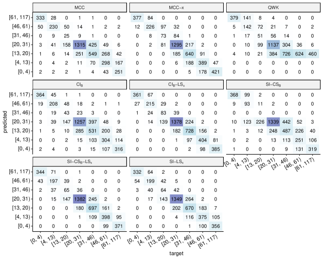
Figure G1: Confusion matrices for UTKFace data for all models mentioned in Table 2. The figure summarizes the true ($x$-axis) vs. the predicted ($y$-axis) classes for the fitted models. The predicted class is the class with the highest predicted probability.

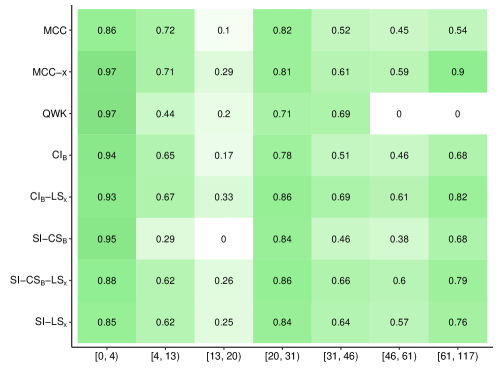
Figure G2: Class-wise accuracies of all models discussed in the main text for the UTKFace data.

References

- Abadi et al. [2015] Martín Abadi et al. TensorFlow: Large-scale machine learning on heterogeneous systems, 2015. URL http://tensorflow.org/. Software available from tensorflow.org.
- Agarwal et al. [2020] Rishabh Agarwal, Nicholas Frosst, Xuezhou Zhang, Rich Caruana, and Geoffrey E Hinton. Neural additive models: Interpretable machine learning with neural nets. arXiv preprint arXiv:2004.13912, 2020.
- Amorim et al. [2018] José P Amorim, Inês Domingues, Pedro Henriques Abreu, and João AM Santos. Interpreting deep learning models for ordinal problems. In Proceedings of the European Symposium on Artificial Neural Networks, 2018.
- Baumann et al. [2020] Philipp FM Baumann, Torsten Hothorn, and David Rügamer. Deep conditional transformation models. arXiv preprint arXiv:2010.07860, 2020.
- Bröcker and Smith [2007] Jochen Bröcker and Leonard A Smith. Scoring probabilistic forecasts: The importance of being proper. Weather and Forecasting, 22(2):382–388, 2007. doi: 10.1175/WAF966.1.
- Cao et al. [2019] Wenzhi Cao, Vahid Mirjalili, and Sebastian Raschka. Rank-consistent ordinal regression for neural networks. arXiv preprint arXiv:1901.07884, 2019.
- Cardoso and Costa [2007] Jaime S Cardoso and Joaquim F Costa. Learning to classify ordinal data: The data replication method. Journal of Machine Learning Research, 8(Jul):1393–1429, 2007. URL https://www.jmlr.org/papers/v8/cardoso07a.html.
- Cheng et al. [2008] Jianlin Cheng, Zheng Wang, and Gianluca Pollastri. A neural network approach to ordinal regression. In 2008 IEEE International Joint Conference on Neural Networks (IEEE World Congress on Computational Intelligence), pages 1279–1284. IEEE, 2008. doi: 10.1109/IJCNN.2008.4633963.
- Chollet et al. [2015] François Chollet et al. Keras. https://keras.io, 2015.
- Chu and Ghahramani [2005] Wei Chu and Zoubin Ghahramani. Gaussian processes for ordinal regression. Journal of Machine Learning Research, 6(Jul):1019–1041, 2005. URL https://www.jmlr.org/papers/v6/chu05a.html.
- Chu and Keerthi [2007] Wei Chu and S Sathiya Keerthi. Support vector ordinal regression. Neural Computation, 19(3):792–815, 2007. doi: 10.1162/neco.2007.19.3.792.
- Cohen [1968] Jacob Cohen. Weighted kappa: nominal scale agreement provision for scaled disagreement or partial credit. Psychological Bulletin, 70(4):213, 1968. doi: 10.1037/h0026256.
- Cortez et al. [2009] Paulo Cortez, António Cerdeira, Fernando Almeida, Telmo Matos, and José Reis. Modeling wine preferences by data mining from physicochemical properties. Decision Support Systems, 47(4):547–553, 2009. doi: 10.1016/j.dss.2009.05.016.
- Das et al. [2018] Abhijit Das, Antitza Dantcheva, and Francois Bremond. Mitigating bias in gender, age and ethnicity classification: a multi-task convolution neural network approach. ECCVW 2018 - EuropeanConference of Computer Vision Workshops, 2018.
- de La Torre et al. [2018] Jordi de La Torre, Domenec Puig, and Aida Valls. Weighted kappa loss function for multi-class classification of ordinal data in deep learning. Pattern Recognition Letters, 105:144–154, 2018. doi: 10.1016/j.patrec.2017.05.018.
- de La Torre et al. [2020] Jordi de La Torre, Aida Valls, and Domenec Puig. A deep learning interpretable classifier for diabetic retinopathy disease grading. Neurocomputing, 396:465–476, 2020.
- Frank and Hall [2001] Eibe Frank and Mark Hall. A simple approach to ordinal classification. In European Conference on Machine Learning, pages 145–156. Springer, 2001. doi: 10.1007/3-540-44795-4˙13.
- Gal and Ghahramani [2016] Yarin Gal and Zoubin Ghahramani. Dropout as a Bayesian approximation: Representing model uncertainty in deep learning. In International Conference on Machine Learning, pages 1050–1059, 2016.
- Gneiting and Raftery [2005] Tilmann Gneiting and Adrian E Raftery. Weather forecasting with ensemble methods. Science, 310(5746):248–249, 2005. doi: 10.1126/science.1115255.
- Gneiting and Raftery [2007] Tilmann Gneiting and Adrian E Raftery. Strictly proper scoring rules, prediction, and estimation. Journal of the American Statistical Association, 102(477):359–378, 2007. doi: 10.1198/016214506000001437.
- Goodfellow et al. [2016] Ian Goodfellow, Yoshua Bengio, and Aaron Courville. Deep learning. MIT press, 2016. doi: 10.1007/s10710-017-9314-z.
- Hothorn [2020] Torsten Hothorn. tram: Transformation Models, 2020. URL https://CRAN.R-project.org/package=tram. R package version 0.5-1.
- Hothorn et al. [2014] Torsten Hothorn, Thomas Kneib, and Peter Bühlmann. Conditional transformation models. Journal of the Royal Statistical Society: Series B: Statistical Methodology, pages 3–27, 2014. doi: 10.1111/rssb.12017.
- Kullback and Leibler [1951] Solomon Kullback and Richard A Leibler. On information and sufficiency. The Annals of Mathematical Statistics, 22(1):79–86, 1951. doi: 10.1214/aoms/1177729694.
- Lakshminarayanan et al. [2017] Balaji Lakshminarayanan, Alexander Pritzel, and Charles Blundell. Simple and scalable predictive uncertainty estimation using deep ensembles. In Advances in Neural Information Processing Systems, pages 6402–6413, 2017.
- Liu et al. [2017a] Hao Liu, Jiwen Lu, Jianjiang Feng, and Jie Zhou. Ordinal deep learning for facial age estimation. IEEE Transactions on Circuits and Systems for Video Technology, 29(2):486–501, 2017a. doi: 10.1109/FG.2017.28.
- Liu et al. [2017b] Yanzhu Liu, Adams Wai-Kin Kong, and Chi Keong Goh. Deep ordinal regression based on data relationship for small datasets. In Proceedings of the International Joint Conference on Artificial Intelligence, pages 2372–2378, 2017b. doi: 10.24963/ijcai.2017/330.
- Liu et al. [2018] Yanzhu Liu, Adams Wai Kin Kong, and Chi Keong Goh. A constrained deep neural network for ordinal regression. In Proceedings of the IEEE Conference on Computer Vision and Pattern Recognition, pages 831–839, 2018. doi: 10.1109/CVPR.2018.00093.
- Liu et al. [2019] Yanzhu Liu, Fan Wang, and Adams Wai Kin Kong. Probabilistic deep ordinal regression based on gaussian processes. In Proceedings of the IEEE International Conference on Computer Vision, pages 5301–5309, 2019. doi: 10.1109/ICCV.2019.00540.
- Manski and Lerman [1977] Charles F Manski and Steven R Lerman. The estimation of choice probabilities from choice based samples. Econometrica: Journal of the Econometric Society, pages 1977–1988, 1977.
- McCullagh [1980] Peter McCullagh. Regression models for ordinal data. Journal of the Royal Statistical Society: Series B (Methodological), 42(2):109–127, 1980. doi: 10.1111/j.2517-6161.1980.tb01109.x.
- Niu et al. [2016] Zhenxing Niu, Mo Zhou, Le Wang, Xinbo Gao, and Gang Hua. Ordinal regression with multiple output cnn for age estimation. In Proceedings of the IEEE Conference on Computer Vision and Pattern Recognition, pages 4920–4928, 2016. doi: 10.1109/CVPR.2016.532.
- Oghina et al. [2012] Andrei Oghina, Mathias Breuss, Manos Tsagkias, and Maarten De Rijke. Predicting imdb movie ratings using social media. In European Conference on Information Retrieval, pages 503–507. Springer, 2012.
- Ribeiro et al. [2016] Marco Tulio Ribeiro, Sameer Singh, and Carlos Guestrin. “Why should I trust you?” explaining the predictions of any classifier. In Proceedings of the 22nd ACM SIGKDD International Conference on Knowledge Discovery and Data Mining, pages 1135–1144, 2016.
- Rudin [2019] Cynthia Rudin. Stop explaining black box machine learning models for high stakes decisions and use interpretable models instead. Nature Machine Intelligence, 1(5):206–215, 2019. doi: 10.1038/s42256-019-0048-x. URL http://www.nature.com/articles/s42256-019-0048-x.
- Rügamer et al. [2020] David Rügamer, Chris Kolb, and Nadja Klein. A unifying network architecture for semi-structured deep distributional learning. arXiv preprint arXiv:2002.05777, 2020.
- Sick et al. [2021] Beate Sick, Torsten Hothorn, and Oliver Dürr. Deep transformation models: Tackling complex regression problems with neural network based transformation models. In Accepted for Proceedings of the 25th International Conference on Pattern Recognition (ICPR), Milan/Online, 2021, 2021.
- Simonyan and Zisserman [2014] Karen Simonyan and Andrew Zisserman. Very deep convolutional networks for large-scale image recognition. arXiv:1409.1556, 09 2014.
- Song and Zhang [Accessed: April 2020] Yang Song and Zhifei Zhang. Utkface data set. https://susanqq.github.io/UTKFace/, Accessed: April 2020.
- Tutz [2011] Gerhard Tutz. Regression for categorical data, volume 34. Cambridge University Press, 2011. doi: 10.1017/CBO9780511842061.
- Vargas et al. [2019] Víctor Manuel Vargas, Pedro Antonio Gutiérrez, and César Hervás. Deep ordinal classification based on the proportional odds model. In International Work-Conference on the Interplay Between Natural and Artificial Computation, pages 441–451. Springer, 2019. doi: 10.1109/BTAS.2016.7791154.
- Vargas et al. [2020] Víctor Manuel Vargas, Pedro Antonio Gutiérrez, and César Hervás-Martínez. Cumulative link models for deep ordinal classification. Neurocomputing, 2020. doi: 10.1016/j.neucom.2020.03.034.
- Wilson and Izmailov [2020] Andrew Gordon Wilson and Pavel Izmailov. Bayesian deep learning and a probabilistic perspective of generalization. arXiv preprint arXiv:2002.08791, 2020.
- Wood [2017] Simon N Wood. Generalized Additive Models: An Introduction with R. Chapman and Hall/CRC, 2 edition, 2017.
- Xie and Pun [2020] Jiu-Cheng Xie and Chi-Man Pun. Deep and Ordinal Ensemble Learning for Human Age Estimation From Facial Images. IEEE Transactions on Information Forensics and Security, 15:2361–2374, 2020. doi: 10.1109/TIFS.2020.2965298. URL https://ieeexplore.ieee.org/document/8957530/.