Abstract

Computing the discrepancy between time series of variable sizes is notoriously challenging. While dynamic time warping (DTW) is popularly used for this purpose, it is not differentiable everywhere and is known to lead to bad local optima when used as a “loss”. Soft-DTW addresses these issues, but it is not a positive definite divergence: due to the bias introduced by entropic regularization, it can be negative and it is not minimized when the time series are equal. We propose in this paper a new divergence, dubbed soft-DTW divergence, which aims to correct these issues. We study its properties; in particular, under conditions on the ground cost, we show that it is a valid divergence: it is non-negative and minimized if and only if the two time series are equal. We also propose a new “sharp” variant by further removing entropic bias. We showcase our divergences on time series averaging and demonstrate significant accuracy improvements compared to both DTW and soft-DTW on 84 time series classification datasets.

1 Introduction

Designing a meaningful discrepancy or “loss” between two sequences of variable lengths and integrating it in an end-to-end differentiable pipeline is challenging. For sequences on finite alphabets, differentiable local alignment kernels (Saigo et al., 2006) and edit distances (McCallum et al., 2012) have been proposed. For sequences on continuous domains, connectionist temporal classification (CTC) is popularly used in speech recognition (Graves et al., 2006). A related approach for time series motivated by geometry is dynamic time warping (DTW), which seeks a minimum-cost alignment between time series and can be computed by dynamic programming in quadratic time (Sakoe and Chiba, 1978). However, DTW is not differentiable everywhere, is sensitive to noise and is known to lead to bad local optima when used as a loss. Soft-DTW (Cuturi and Blondel, 2017) addresses these issues by replacing the minimum over alignments with a soft minimum, which has the effect of inducing a probability distribution over all alignments. Despite considering all alignments, it is shown that soft-DTW can still be computed by dynamic programming in the same complexity. Since then, soft-DTW has been successfully applied for audio to music score alignment (Mensch and Blondel, 2018), video segmentation (Chang et al., 2019), spatial-temporal sequences (Janati et al., 2020), and end-to-end differentiable text-to-speech synthesis (Donahue et al., 2020), to name but a few examples. Soft-DTW is included in popular R and Python packages for time series analysis (Sardá-Espinosa, 2017; Tavenard et al., 2020).

In this paper, we show that, despite recent successes, soft-DTW has some limitations which have been overlooked in the literature. First, it can be negative, which is a nuisance when used as a loss. Second, and more problematically, when used with a squared Euclidean cost, we show that it is never minimized when the two time series are equal. Put differently, given an input time series, the closest time series in the soft-DTW sense is never the input time series. This is due to the entropic bias introduced by replacing the minimum with a soft one. We propose in this paper a new divergence, dubbed soft-DTW divergence, which is based on soft-DTW but corrects for these issues. We study its properties; in particular, under condition on the ground cost, we show that it is a valid divergence: it is non-negative and it is minimized if and only if the two time series are equal. Our approach is related to Sinkhorn divergences (Ramdas et al., 2017; Genevay et al., 2018; Feydy et al., 2019), which use similar correction terms as we do for optimal transport distances, but our proof techniques are completely different. We also propose a new “sharp” variant by further removing entropic bias. We showcase our divergences on time series averaging and demonstrate significant accuracy improvements compared to both DTW and soft-DTW on 84 time series classification datasets.

The rest of the paper is organized as follows. After reviewing some background in §2, we introduce the soft-DTW divergence and its “sharp” variant in §3. We study their properties and limit behavior. We study their empirical performance in §4 with experiments on time series averaging, interpolation and classification.

2 Background

2.1 Dynamic time warping

Let ${\bm{X}}\in\mathbb{R}^{m\times d}$ and ${\bm{Y}}\in\mathbb{R}^{n\times d}$ be two $d$-dimensional time series of lengths $m$ and $n$. We denote their elements by ${\bm{x}}_{i}\in\mathbb{R}^{d}$ and ${\bm{y}}_{j}\in\mathbb{R}^{d}$, for $i\in[m]$ and $j\in[n]$. We say that $\bm{A}\in\{0,1\}^{m\times n}$ is an alignment matrix between ${\bm{X}}$ and ${\bm{Y}}$ when $[\bm{A}]_{i,j}=1$ if ${\bm{x}}_{i}$ is aligned with ${\bm{y}}_{j}$ and $0$ otherwise. We say that $\bm{A}$ is a monotonic alignment matrix if the ones in $\bm{A}$ form a path starting from the upper-left corner $(1,1)$ that connects the lower-right corner $(m,n)$ using only $\downarrow$, $\rightarrow$, $\searrow$ moves. We denote the set of all such monotonic alignment matrices by $\mathcal{A}(m,n)\subset\{0,1\}^{m\times n}$. The cardinality $|\mathcal{A}(m,n)|$ grows exponentially in $\min(m,n)$ and is equal to the Delannoy number, $\text{Delannoy}(m-1,n-1)$, named after French amateur mathematician Henri Delannoy (Sulanke, 2003; Banderier and Schwer, 2005).

Let $C\colon\mathbb{R}^{m\times d}\times\mathbb{R}^{n\times d}\to\mathbb{R}^{m\times n}$ be a function which maps ${\bm{X}}\in\mathbb{R}^{m\times d}$ and ${\bm{Y}}\in\mathbb{R}^{n\times d}$ to a distance or cost matrix ${\bm{C}}=C({\bm{X}},{\bm{Y}})\in\mathbb{R}^{m\times n}$. A popular choice is the squared Euclidean cost

$$[C({\bm{X}},{\bm{Y}})]_{i,j}=\frac{1}{2}\|{\bm{x}}_{i}-{\bm{y}}_{j}\|^{2}_{2}\quad i\in[m],j\in[n].$$ (1)

The Frobenius inner product $\langle\bm{A},{\bm{C}}\rangle\coloneqq\text{Trace}({\bm{C}}^{\top}\bm{A})$ between ${\bm{C}}$ and $\bm{A}$ is the sum of the costs along the alignment (Figure 1). Dynamic time warping (Sakoe and Chiba, 1978) can then be naturally formulated as the minimum cost among all possible alignments,

$$\textsc{dtw}({\bm{C}})\coloneqq\min_{\bm{A}\in\mathcal{A}(m,n)}\langle\bm{A},{\bm{C}}\rangle.$$ (2)

The corresponding optimal alignment (not necessarily unique) is then

$$\bm{A}^{\star}({\bm{C}})\in\operatorname*{argmin}_{\bm{A}\in\mathcal{A}(m,n)}\langle\bm{A},{\bm{C}}\rangle.$$ (3)

Despite the exponential number of alignments, (2) and (3) can be computed in $O(mn)$ time using dynamic programming and backtracking, respectively. The quantity $\textsc{dtw}(C({\bm{X}},{\bm{Y}}))$ is popularly used as a discrepancy measure between time series in numerous applications. In the rest of the paper, we will make the following assumptions about the ground cost $C$:

• A.1. $C({\bm{X}},{\bm{Y}})\geq{\bm{0}}_{m\times n}$ (non-negativity),

• A.2. $[C({\bm{X}},{\bm{X}})]_{i,i}=0$ for all $i\in[m]$,

• A.3. $C({\bm{X}},{\bm{Y}})=C({\bm{Y}},{\bm{X}})^{\top}$ (symmetry).

The properties of dtw under these assumptions are summarized in Table 1. Note that dtw is minimized at ${\bm{X}}={\bm{Y}}$ but this may not be the unique minimum.

Table 1: Properties of time-series losses under assumptions A.1-A.3 and differentiability of $C$. For the soft-DTW divergence, we prove non-negativity and “minimized at ${\bm{X}}={\bm{Y}}$” using the cost (16) and one-dimensional absolute value (17) (cf. Proposition 3). For the soft-DTW and sharp divergences with the squared Euclidean cost (1), we only prove that ${\bm{X}}={\bm{Y}}$ is a stationary point (cf. Proposition 3)

	Non-negativity	Minimized at ${\bm{X}}={\bm{Y}}$	Symmetry	Differentiable everywhere
DTW	$\checkmark$	$\checkmark$	$\checkmark$	$\times$
Soft-DTW	$\times$	$\times$	$\checkmark$	$\checkmark$
Sharp soft-DTW	$\checkmark$	$\times$	$\checkmark$	$\checkmark$
Soft-DTW divergence	$\checkmark$	$\checkmark$	$\checkmark$	$\checkmark$
Sharp divergence	$\checkmark$	$\checkmark$	$\checkmark$	$\checkmark$
Mean-cost divergence	$\checkmark$	$\checkmark$	$\checkmark$	$\checkmark$

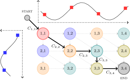
Figure 1: An alignment between two time series ${\bm{X}}\in\mathbb{R}^{m\times d}$ and ${\bm{Y}}\in\mathbb{R}^{n\times d}$ corresponds to a path in a directed acyclic graph (DAG) and can be encoded as a binary matrix $\bm{A}\in\{0,1\}^{m\times n}$. The sum of the costs along the path is then $\langle\bm{A},{\bm{C}}\rangle$. DTW seeks a minimum cost alignment, while soft-DTW seeks the soft minimum cost alignment. The latter induces a Gibbs distribution over all alignments.

2.2 Soft dynamic time warping

Definitions.

In order to obtain a fully differentiable discrepancy measure between time series, Cuturi and Blondel (2017) proposed to replace the min operator in (2) by a smooth one,

$$\underset{x\in\mathcal{S}}{\text{min}_{\gamma}}~{}f(x)\coloneqq-\gamma\log\sum_{x\in\mathcal{S}}\exp(-f(x)/\gamma),$$ (4)

where $\gamma>0$ is a parameter which controls the trade-off between approximation and smoothness. For convenience, we define the extension $\text{min}_{0}\coloneqq\min$. The resulting “soft” dynamic time warping formulation is

$$\textsc{sdtw}_{\gamma}({\bm{C}}) \coloneqq\underset{\bm{A}\in\mathcal{A}(m,n)}{\text{min}_{\gamma}}\langle\bm{A},{\bm{C}}\rangle$$ (5)

$$=-\gamma\log\sum_{\bm{A}\in\mathcal{A}(m,n)}\exp(-\langle\bm{A},{\bm{C}}\rangle/\gamma).$$ (6)

Instead of only considering the minimum-cost alignment as in (2), (6) induces a Gibbs distribution over alignments. The probability of $\bm{A}$ given ${\bm{C}}\in\mathbb{R}^{m\times n}$ is

$$\mathbb{P}_{\gamma}(\bm{A};{\bm{C}})\coloneqq\frac{\exp(-\langle\bm{A},{\bm{C}}\rangle/\gamma)}{\sum_{\bm{A}^{\prime}\in\mathcal{A}(m,n)}\langle-\langle\bm{A}^{\prime},{\bm{C}}\rangle/\gamma)}\in(0,1].$$ (7)

We can see (6) as the negative log-partition of (7). For convenience, we also gather the probabilities of all possible alignments in a vector

$$\bm{p}_{\gamma}({\bm{C}})\coloneqq(\mathbb{P}_{\gamma}(\bm{A};{\bm{C}}))_{\bm{A}\in\mathcal{A}(m,n)}\in\triangle^{|A(m,n)|},$$ (8)

where $\triangle^{k}\coloneqq\{\bm{p}\in\mathbb{R}^{k}\colon\bm{p}\geq{\bm{0}}_{k},\bm{p}^{\top}{\bm{1}}_{k}=1\}$ is the probability simplex. Let $A$ be a random variable distributed according to (7). The expected alignment matrix under the Gibbs distribution induced by ${\bm{C}}$ is

$$\bm{E}_{\gamma}({\bm{C}})\coloneqq\mathbb{E}_{\gamma}[A;{\bm{C}}]=\sum_{\bm{A}\in\mathcal{A}(m,n)}\mathbb{P}_{\gamma}(\bm{A};{\bm{C}})\bm{A}\in(0,1]^{m\times n}.$$ (9)

Note that because the matrices in $\mathcal{A}(m,n)$ are binary ones, $[\bm{E}_{\gamma}({\bm{C}})]_{i,j}$ is also equal to the marginal probability $\mathbb{P}_{\gamma}(A_{i,j}=1;{\bm{C}})$, i.e., the probability that any of the paths goes through the cell $(i,j)$.

Computation.

Surprisingly, even though (6) contains a sum over all $\bm{A}$ in $\mathcal{A}(m,n)$, it can be computed in $O(mn)$ time by simply replacing the $\min$ operator with $\text{min}_{\gamma}$ in the original dynamic programming recursion (Cuturi and Blondel, 2017). See also Algorithm 1 in Appendix A. The equivalence between (6) and this “locally smoothed” recursion was later formally proved using the associativity of the $\text{min}_{\gamma}$ operator (Mensch and Blondel, 2018). The expected alignment can also be computed in $O(mn)$ time by backpropagation through the dynamic programming recursion (Cuturi and Blondel, 2017). See also Algorithm 2 in Appendix A.

Properties.

The following proposition summarizes known properties of $\textsc{sdtw}_{\gamma}$ (Cuturi and Blondel, 2017; Mensch and Blondel, 2018). Properties of $\textsc{sdtw}_{\gamma}$

The following properties hold for all ${\bm{C}}\in\mathbb{R}^{m\times n}$.

1. Gradient: $\textsc{sdtw}_{\gamma}({\bm{C}})$ is differentiable everywhere and its gradient is the expected alignment,

   $$\nabla_{\bm{C}}\textsc{sdtw}_{\gamma}({\bm{C}})=\bm{E}_{\gamma}({\bm{C}})\in(0,1]^{m\times n}.$$ (10)

2. Concavity: $\textsc{sdtw}_{\gamma}({\bm{C}})$ is concave in ${\bm{C}}$.

3. Variational form: letting $H(\bm{p})=-\langle\bm{p},\log\bm{p}\rangle$,

   $$\textsc{sdtw}_{\gamma}({\bm{C}})=\min_{\bm{p}\in\triangle^{|\mathcal{A}(m,n)|}}\langle\bm{p},\bm{s}({\bm{C}})\rangle-\gamma H(\bm{p})$$ (11)

   where $\bm{s}({\bm{C}})\coloneqq(\langle\bm{A},{\bm{C}}\rangle)_{\bm{A}\in\mathcal{A}(mmn)}\in\mathbb{R}^{|\mathcal{A}(m,n)|}$.

4. Scaling: $\textsc{sdtw}_{\gamma}({\bm{C}})=\gamma\textsc{sdtw}_{1}({\bm{C}}/\gamma)$, $\bm{E}_{\gamma}({\bm{C}})=\bm{E}_{1}({\bm{C}}/\gamma)$ and $\bm{p}_{\gamma}({\bm{C}})=\bm{p}_{1}({\bm{C}}/\gamma)$.

5. Asymptotics: $\textsc{dtw}({\bm{C}})\xleftarrow[0\leftarrow\gamma]{}\textsc{sdtw}_{\gamma}({\bm{C}})$ and $\bm{A}^{\star}({\bm{C}})\xleftarrow[0\leftarrow\gamma]{}\bm{E}_{\gamma}({\bm{C}})$.

6. Lower and upper bounds:

   $$\textsc{dtw}({\bm{C}})-\gamma\log|\mathcal{A}(m,n)|\leq\textsc{sdtw}_{\gamma}({\bm{C}})\leq\textsc{dtw}({\bm{C}}).$$ (12)

Note that $\textsc{sdtw}_{\gamma}(C({\bm{X}},{\bm{Y}}))$ is generally neither convex nor concave in ${\bm{X}}$ and ${\bm{Y}}$, as is the case when $C$ is the squared Euclidean cost (1). A notable exception is $C({\bm{X}},{\bm{Y}})=-{\bm{X}}{\bm{Y}}^{\top}$, for which $\textsc{sdtw}_{\gamma}(C({\bm{X}},{\bm{Y}}))$ is concave in ${\bm{X}}$ and ${\bm{Y}}$ (separately).

Use as a loss function.

The differentiability of $\textsc{sdtw}_{\gamma}$ makes it particularly suitable to use as a loss function between time series, of potentially variable lengths. An example of application is the computation of Fréchet means (1948) with respect to $\textsc{sdtw}_{\gamma}$. Specifically, given a set of $k$ time series ${\bm{Y}}_{1}\in\mathbb{R}^{n_{1}\times d}$, $\dots$, ${\bm{Y}}_{k}\in\mathbb{R}^{n_{k}\times d}$, we compute its average (barycenter) according to $\textsc{sdtw}_{\gamma}$ by solving

$$\operatorname*{argmin}_{{\bm{X}}\in\mathbb{R}^{m\times d}}\sum_{i=1}^{k}w_{i}~{}\textsc{sdtw}_{\gamma}(C({\bm{X}},{\bm{Y}}_{i})),$$ (13)

where $\bm{w}=(w_{1},\dots,w_{k})\in\mathbb{R}^{k}$ is a vector of pre-defined weights. When the time series ${\bm{Y}}_{1},\dots,{\bm{Y}}_{k}$ have different lengths, a typical choice would be $w_{i}=1/n_{i}$, to compensate for the fact that $\textsc{sdtw}_{\gamma}$ increases with the length of the time series. Although it is non-convex, objective (13) can be solved approximately by gradient-based methods. Compared to DTW barycenter averaging (DBA) (Petitjean et al., 2011), it was shown that smoothing helps to avoid bad local optima. Using the chain rule and item 1 of Proposition 2.2, the gradient of $\textsc{sdtw}_{\gamma}(C({\bm{X}},{\bm{Y}}))$ w.r.t. ${\bm{X}}$ is

$$\nabla_{\bm{X}}\textsc{sdtw}_{\gamma}(C({\bm{X}},{\bm{Y}}))=(J_{\bm{X}}C({\bm{X}},{\bm{Y}}))^{\top}\bm{E}_{\gamma}({\bm{C}}({\bm{X}},{\bm{Y}})).$$ (14)

Here, we assume that $C$ is differentiable and $J_{\bm{X}}$ denotes the Jacobian matrix of ${\bm{C}}({\bm{X}},{\bm{Y}})$ w.r.t. ${\bm{X}}$, a linear map from $\mathbb{R}^{m\times d}$ to $\mathbb{R}^{m\times n}$ (its transpose is a linear map from $\mathbb{R}^{m\times n}$ to $\mathbb{R}^{m\times d}$).

2.3 Global alignment kernel

Although it was introduced before soft dynamic time warping, the global alignment kernel (Cuturi et al., 2007) can be naturally expressed using $\textsc{sdtw}_{\gamma}$ as

$$K_{\gamma}^{C}({\bm{X}},{\bm{Y}})\coloneqq\exp(-\textsc{sdtw}_{1}(C({\bm{X}},{\bm{Y}})/\gamma)).$$ (15)

Using a constructive proof, it was shown that (15) is a positive definite (p.d.) kernel under certain cost functions and in particular with

$$[C({\bm{X}},{\bm{Y}})]_{i,j}=\delta({\bm{x}}_{i},{\bm{y}}_{i})+\log(2-\exp(-\delta({\bm{x}}_{i},{\bm{y}}_{i})),$$ (16)

where $\delta({\bm{x}},{\bm{y}})\coloneqq\frac{1}{2}\|{\bm{x}}-{\bm{y}}\|^{2}_{2}$. In the one-dimensional case ($d=1$), we show in Appendix B.4 that

$$[C({\bm{X}},{\bm{Y}})]_{i,j}=\|{\bm{x}}_{i}-{\bm{y}}_{j}\|_{1},$$ (17)

also has the property that the kernel (15) is p.d. Using these costs, (15) can be used in any kernel method, such as support vector machines. The positive definiteness of (15) using the squared Euclidean cost (1) has to our knowledge not been proved or disproved yet.

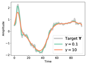
Figure 2: Denoising effect of soft-DTW. We show the result of $\operatorname*{argmin}_{{\bm{X}}}\textsc{sdtw}_{\gamma}(C({\bm{X}},{\bm{Y}}))$, solved by L-BFGS with ${\bm{X}}={\bm{Y}}$ as initialization, for two values of $\gamma$. As stated in Proposition 3, $\textsc{sdtw}_{\gamma}$ with $\gamma>0$ and squared Euclidean cost never achieves its minimum at ${\bm{X}}={\bm{Y}}$. While this denoising can be useful, this means that $\textsc{sdtw}_{\gamma}$ is not a valid divergence.

3 New differentiable divergences

In this section, we begin by pointing out potential limitations of soft-DTW. We then introduce two new divergences, the soft-DTW divergence and its sharp variant, which aim to correct for these limitations. We study their properties and limit behavior.

Limitations of soft-DTW.

Despite recent empirical successes, soft-DTW has some inherent limitations that were not discussed in previous works. The following proposition clarifies these limitations. Limitations of $\textsc{sdtw}_{\gamma}$

The following holds.

1. For all ${\bm{C}}\in\mathbb{R}^{m\times n}$, $\gamma\mapsto\textsc{sdtw}_{\gamma}({\bm{C}})$ is non-increasing, concave, and diverges to $-\infty$ when $\gamma\rightarrow+\infty$. In particular, there exists $\gamma_{0}\in[0,\infty)$ such that $\textsc{sdtw}_{\gamma}({\bm{C}})\leq 0$ for all $\gamma\geq\gamma_{0}$.

2. For all cost functions $C$ satisfying A.2, ${\bm{X}}\in\mathbb{R}^{m\times d}$ and $\gamma\in[0,\infty)$, $\textsc{sdtw}_{\gamma}(C({\bm{X}},{\bm{X}}))\leq 0$.

3. For the squared Euclidean cost (1) and any $\gamma\in(0,\infty)$, the minimum of $\textsc{sdtw}_{\gamma}(C({\bm{X}},{\bm{Y}}))$ is not achieved at ${\bm{X}}={\bm{Y}}$.

A proof is given in Appendix B.3. Proposition 3 shows that that there exists values of $\gamma$ or ${\bm{C}}$ for which $\textsc{sdtw}_{\gamma}({\bm{C}})$ is negative. Non-negativity is a useful property of divergences and the fact that $\textsc{sdtw}_{\gamma}$ does not satisfy it can be a nuisance. More problematic is the fact that $\textsc{sdtw}_{\gamma}(C({\bm{X}},{\bm{Y}}))$ is not minimized at ${\bm{X}}={\bm{Y}}$. This is illustrated in Figure 2. While the denoising effect of soft-DTW can be useful, we would expect a proper differentiable divergence to be zero when the two time series are equal.

Soft-DTW divergences.

To address these issues, we propose to use for all ${\bm{X}}\in\mathbb{R}^{m\times d}$ and ${\bm{Y}}\in\mathbb{R}^{n\times d}$

$$D_{\gamma}^{C}({\bm{X}},{\bm{Y}})\coloneqq~{} \textsc{sdtw}_{\gamma}(C({\bm{X}},{\bm{Y}}))$$ (18)

$$-\frac{1}{2} \textsc{sdtw}_{\gamma}(C({\bm{X}},{\bm{X}}))$$ (19)

$$-\frac{1}{2} \textsc{sdtw}_{\gamma}(C({\bm{Y}},{\bm{Y}})).$$ (20)

Since it is based on soft-DTW, we call it the soft-DTW divergence. Sinkhorn divergences (Ramdas et al., 2017; Genevay et al., 2018; Feydy et al., 2019), which are divergences between probability measures based on entropy-regularized optimal transport, use similar correction terms.

Sharp divergences.

The variational form of $\textsc{sdtw}_{\gamma}$ (Proposition 2.2) implies that it can be decomposed as the sum of a cost term and an entropy term,

$$\textsc{sdtw}_{\gamma}({\bm{C}})=\langle\bm{E}_{\gamma}({\bm{C}}),{\bm{C}}\rangle-\gamma H(\bm{p}_{\gamma}({\bm{C}})).$$ (21)

On the other hand, we have

$$\textsc{dtw}({\bm{C}})=\langle\bm{A}^{\star}({\bm{C}}),{\bm{C}}\rangle.$$ (22)

Since $\bm{E}_{\gamma}({\bm{C}})\to\bm{A}^{\star}({\bm{C}})$ when $\gamma\to 0$, this suggests a new discrepancy measure,

$$\textsc{sharp}_{\gamma}({\bm{C}})\coloneqq\langle\bm{E}_{\gamma}({\bm{C}}),{\bm{C}}\rangle.$$ (23)

It is the directional derivative of $\textsc{sdtw}_{\gamma}({\bm{C}})$ in the direction of ${\bm{C}}$, since $\bm{E}_{\gamma}({\bm{C}})=\nabla_{\bm{C}}\textsc{sdtw}_{\gamma}({\bm{C}})$. Inspired by Luise et al. (2018), who studied a similar idea in an optimal transport context,we call it sharp soft-DTW, since it removes the entropic regularization term $-\gamma H(\bm{p}_{\gamma}({\bm{C}}))$ from (21). Its gradient is equal to

$$\nabla_{\bm{C}}\textsc{sharp}_{\gamma}({\bm{C}})=\bm{E}_{\gamma}({\bm{C}})+\frac{1}{\gamma}\nabla^{2}_{\bm{C}}\textsc{sdtw}_{\gamma}({\bm{C}}){\bm{C}}\in\mathbb{R}^{m\times n},$$ (24)

where $\nabla^{2}_{\bm{C}}\textsc{sdtw}_{\gamma}({\bm{C}}){\bm{C}}$ is a Hessian-vector product (that can be computed efficiently, as we detail below). The gradient w.r.t. ${\bm{X}}$ is obtained by the chain rule, similarly to (14). Although $\textsc{sharp}_{\gamma}$ is trivially non-negative, it suffers from the same issue as $\textsc{sdtw}_{\gamma}$, namely, $\textsc{sharp}_{\gamma}(C({\bm{X}},{\bm{Y}}))$ is not minimized at ${\bm{X}}={\bm{Y}}$. We therefore propose to use instead

$$S_{\gamma}^{C}({\bm{X}},{\bm{Y}})\coloneqq~{} \textsc{sharp}_{\gamma}(C({\bm{X}},{\bm{Y}}))$$ (25)

$$-\frac{1}{2} \textsc{sharp}_{\gamma}(C({\bm{X}},{\bm{X}}))$$ (26)

$$-\frac{1}{2} \textsc{sharp}_{\gamma}(C({\bm{Y}},{\bm{Y}})).$$ (27)

We call it the sharp soft-DTW divergence.

Validity.

We remind the reader that in mathematics, a divergence $D$ is a function that is non-negative ($D({\bm{X}},{\bm{Y}})\geq 0$ for any ${\bm{X}},{\bm{Y}}$) and that satisfies the identify of indiscernibles ($D({\bm{X}},{\bm{Y}})=0$ if and only if ${\bm{X}}={\bm{Y}}$). By construction, we have $D_{\gamma}^{C}({\bm{X}},{\bm{X}})=0$ and $S_{\gamma}^{C}({\bm{X}},{\bm{X}})=0$ for all ${\bm{X}}\in\mathbb{R}^{m\times d}$. Moreover, the following result shows that $D_{\gamma}^{C}$ is a valid divergence, under some assumptions on the cost $C$. Valid divergence.

Let $\gamma>0$. If $C$ is the cost defined in (16) with $d\in\mathbb{N}$, or, if $C$ is the absolute value (17) with $d=1$, then $D_{\gamma}^{C}({\bm{X}},{\bm{Y}})\geq 0$ for all ${\bm{X}}\in\mathbb{R}^{m\times d}$ and ${\bm{Y}}\in\mathbb{R}^{n\times d}$, and $D_{\gamma}^{C}({\bm{X}},{\bm{Y}})=0$ if and only if ${\bm{X}}={\bm{Y}}$. Therefore, $D_{\gamma}^{C}$ is a valid divergence. A proof is given in Appendix B.4. This implies that, for the costs (16) and (17), $D_{\gamma}^{C}({\bm{X}},{\bm{Y}})$ is uniquely minimized at ${\bm{X}}={\bm{Y}}$. The proof relies on the fact that the global alignment kernel (15) is positive definite under these costs. Unfortunately, since the positive definiteness of (15) under the squared Euclidean cost (1) has not been proved or disproved, the same proof technique does not apply. Nevertheless, we can prove the following. Stationary point under cost (1)

If $C$ is the squared Euclidean cost (1), then ${\bm{X}}={\bm{Y}}$ is a stationary point of $D_{\gamma}^{C}({\bm{X}},{\bm{Y}})$ and $S_{\gamma}^{C}({\bm{X}},{\bm{Y}})$ w.r.t. ${\bm{X}}\in\mathbb{R}^{n\times d}$ for all ${\bm{Y}}\in\mathbb{R}^{n\times d}$. A proof is given in Appendix B.6. Based on Proposition 3 and ample numerical evidence (cf. Appendix B.5), we conjecture that $D_{\gamma}^{C}({\bm{X}},{\bm{Y}})$ and $S_{\gamma}^{C}({\bm{X}},{\bm{Y}})$ are also non-negative under the squared Euclidean cost.

Asymptotic behavior.

We now study the behavior of our divergences in the zero and infinite temperature limits, i.e., when $\gamma\to 0$ and $\gamma\to\infty$. As we saw, $\bm{E}_{\gamma}({\bm{C}})$ is the expected alignment matrix under the Gibbs distribution $\mathbb{P}_{\gamma}(\bm{A};{\bm{C}})$. Let $A$ be a random alignment matrix uniformly distributed over $\mathcal{A}(m,n)$, i.e., independent of the cost matrix ${\bm{C}}$. Replacing $\bm{E}_{\gamma}({\bm{C}})$ with $\mathbb{E}[A]$ in (23), we obtain the mean cost, the average of the cost along all possible paths,

$$\text{{mean\_cost}}({\bm{C}}) \coloneqq\langle\mathbb{E}[A],{\bm{C}}\rangle$$ (28)

$$=\frac{1}{|\mathcal{A}(m,n)|}\sum_{\bm{A}\in\mathcal{A}(m,n)}\langle\bm{A},{\bm{C}}\rangle.$$ (29)

We also define the mean-cost divergence,

$$M^{C}({\bm{X}},{\bm{Y}}) \coloneqq\text{{mean\_cost}}(C({\bm{X}},{\bm{Y}}))$$ (30)

$$-\frac{1}{2}\text{{mean\_cost}}(C({\bm{X}},{\bm{X}}))$$ (31)

$$-\frac{1}{2}\text{{mean\_cost}}(C({\bm{Y}},{\bm{Y}})).$$ (32)

It bears some similarity with energy distances (Baringhaus and Franz, 2004; Székely et al., 2004), with the key difference that the probability distribution is over the alignments, not over the time series.

We now show that our proposed divergences are all intimately related through their asymptotic behavior, and that $D_{\gamma}^{C}$ and $S_{\gamma}^{C}$ share the same limits to the right when $m=n$ but not when $m\neq n$. Limits w.r.t. $\gamma$

For all ${\bm{C}}=C({\bm{X}},{\bm{Y}})\in\mathbb{R}^{m\times n}$, $m=n$:

$$\textsc{dtw}({\bm{C}})\xleftarrow[0\leftarrow\gamma]{}D_{\gamma}^{C}({\bm{X}},{\bm{Y}})\xrightarrow[\gamma\to\infty]{}M^{C}({\bm{X}},{\bm{Y}}).$$ (33)

For all ${\bm{C}}=C({\bm{X}},{\bm{Y}})\in\mathbb{R}^{m\times n}$, $m\neq n$:

$$\textsc{dtw}({\bm{C}})\xleftarrow[0\leftarrow\gamma]{}D_{\gamma}^{C}({\bm{X}},{\bm{Y}})\xrightarrow[\gamma\to\infty]{}\infty.$$ (34)

For all ${\bm{C}}=C({\bm{X}},{\bm{Y}})\in\mathbb{R}^{m\times n}$:

$$\textsc{dtw}({\bm{C}})\xleftarrow[0\leftarrow\gamma]{}S_{\gamma}^{C}({\bm{X}},{\bm{Y}})\xrightarrow[\gamma\to\infty]{}M^{C}({\bm{X}},{\bm{Y}}).$$ (35)

Note that the mean-cost divergence was obtained mostly as a side product of our limit case analysis. As we show in our experiments, it performs worse than the (sharp) soft-DTW divergence in practice. Therefore we do not recommend it in practice.

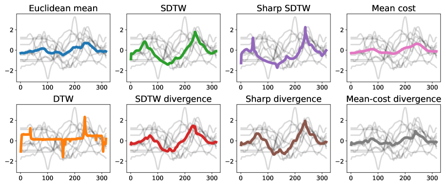
Figure 3: Average of $10$ time series ${\bm{Y}}_{1},\dots,{\bm{Y}}_{10}$, on the uWaveGestureLibrary_Y dataset.

Computation.

The value, gradient, directional derivative and Hessian product of $\textsc{sdtw}_{\gamma}({\bm{C}})$ for ${\bm{C}}\in\mathbb{R}^{m\times n}$ can all be computed in $O(mn)$ time (Cuturi and Blondel, 2017; Mensch and Blondel, 2018). Therefore, both $D_{\gamma}^{C}({\bm{X}},{\bm{Y}})$ and $S_{\gamma}^{C}({\bm{X}},{\bm{Y}})$ take $O(\max\{m,n\}^{2})$ time to compute. Sharp divergences take roughly twice more time to compute, as computing a Hessian-vector product requires one more pass through the dynamic programming recursion. The mean alignment and mean cost can also both be computed in $O(mn)$ time. We detail all algorithms in Appendix A.

Comparison with Sinkhorn divergences.

Since our proposed divergences use similar correction terms as Sinkhorn divergences, we briefly review them and discuss their differences. Given two input probability measures $\bm{\alpha}\in\triangle^{m}$ and $\bm{\beta}\in\triangle^{n}$, entropy-regularized optimal transport is now commonly defined as

$$\textsc{OT}_{\gamma}(\bm{\alpha},\bm{\beta})\coloneqq\min_{\bm{T}\in\mathcal{U}(\bm{\alpha},\bm{\beta})}\langle\bm{T},{\bm{C}}\rangle+\gamma\text{KL}(\bm{T}||\bm{\alpha}\otimes\bm{\beta}),$$ (36)

where KL is the Kullback-Leibler divergence and $\mathcal{U}(\bm{\alpha},\bm{\beta})$ is the so-called transportation polytope (Peyré et al., 2019). To address the entropic bias of $\textsc{OT}_{\gamma}$, Sinkhorn divergences include correction terms, i.e., they are defined as $(\bm{\alpha},\bm{\beta})\mapsto\textsc{OT}_{\gamma}(\bm{\alpha},\bm{\beta})-\frac{1}{2}\textsc{OT}_{\gamma}(\bm{\alpha},\bm{\alpha})-\frac{1}{2}\textsc{OT}_{\gamma}(\bm{\beta},\bm{\beta})$. There are however two important differences between $\textsc{OT}_{\gamma}$ and $\textsc{sdtw}_{\gamma}(C(\cdot,\cdot))$. First, the former is convex in its inputs (separately) while the latter is not. This means that the proof technique for non-negativity of Sinkhorn divergences (Feydy et al., 2019) does not apply to the soft-DTW divergence. Indeed our proof technique for Proposition 3 is completely different than for Sinkhorn divergences. Second, the entropic regularization in $\textsc{sdtw}_{\gamma}$ is on the probability distribution (Proposition 1), not on the soft alignment, as is the case for the transportation map $\bm{T}$ in (36). Contrary to Sinkhorn divergences, the soft-DTW and sharp divergences are non-convex in their inputs. For time-series averaging, an initialization scheme that works well in practice is to use the $\textsc{sdtw}_{\gamma}$ solution as initialization, itself initialized from the Euclidean mean.

4 Experimental results

Throughout this section, we use the UCR (University of California, Riverside) time series classification archive (Chen et al., 2015). We use a subset containing 84 datasets encompassing a wide variety of fields (astronomy, geology, medical imaging) and lengths. Datasets include class information (up to 60 classes) for each time series and are split into train and test sets. Due to the large number of datasets in the UCR archive, we choose to report only a summary of our results in the main manuscript. Detailed results are included in the appendix for interested readers. In all experiments, we use the squared Euclidean cost (1). Our Python source code is available on github.

4.1 Time series averaging

Experimental setup.

To investigate the effect of our divergences on time series averaging, we replace $\textsc{sdtw}_{\gamma}$ in objective (13) with our divergences. For this task, we focus on a visual comparison and refrain from reporting quantitative results, since the choice of evaluation metric necessarily favors one divergence over others. For each dataset, we pick $10$ time series ${\bm{Y}}_{1},\dots,{\bm{Y}}_{10}$ randomly. Since the time series all have the same length, we use uniform weights $w_{1}=\dots=w_{k}=1$. To approximately minimize the objective function, we use $200$ iterations of L-BFGS (Liu and Nocedal, 1989). Because the objective is non-convex in ${\bm{X}}$, initialization is important. For dtw, $\textsc{sdtw}_{\gamma}$, $\textsc{sharp}_{\gamma}$ and mean_cost, we use the Euclidean mean as initialization and set $\gamma=1$. For $D_{\gamma}^{C}$, $S_{\gamma}^{C}$ and $M^{C}$, we use as initialization the solution of their “biased couterpart”, i.e., $\textsc{sdtw}_{\gamma}$, $\textsc{sharp}_{\gamma}$, mean_cost, respectively, and we set $\gamma=10$.

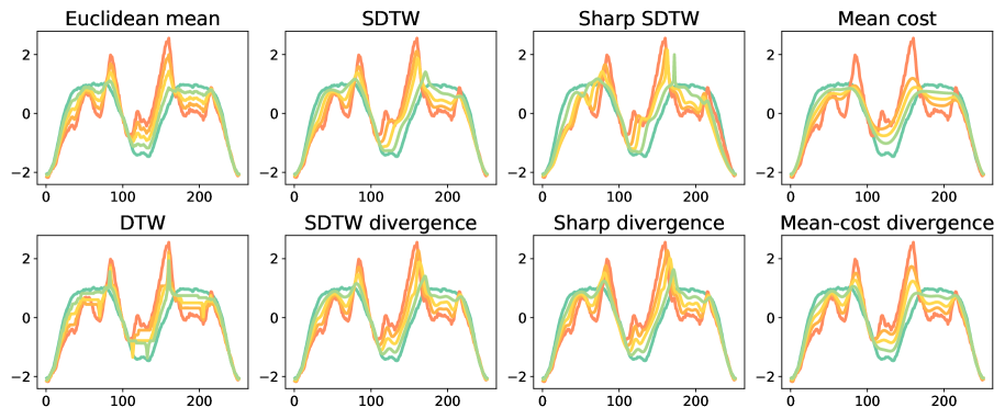
Figure 4: Interpolation between two time series ${\bm{Y}}_{1}$ (red) and ${\bm{Y}}_{2}$ (dark green), from the ArrowHead dataset.

Results.

We show the time series averages obtained on the uWaveGestureLibrary_Y dataset in Figure 3. With DTW, the obtained average does not match well the time series, confirming the conclusion of Cuturi and Blondel (2017). This is because the objective is both highly non-convex and non-smooth, rendering optimization difficult, despite the use of Euclidean mean as initialization. On the other hand, the averages obtained by other divergences appear to match the time series much better, thanks to the smoothness of their objective function. We observe that $D_{\gamma}^{C}$ (soft-DTW divergence), $S_{\gamma}^{C}$ (sharp divergence) and $M^{C}$ (mean-cost divergence) produce different results from their biased counterpart, $\textsc{sdtw}_{\gamma}$ (soft-DTW), $\textsc{sharp}_{\gamma}$ (sharp soft-DTW) and mean_cost (mean cost), respectively. This is to be expected, since the variable ${\bm{X}}$ with respect to which we minimize is involved in the correcting term using $C({\bm{X}},{\bm{X}})$. The averages obtained with $\textsc{sharp}_{\gamma}$ and $S_{\gamma}^{C}$ tend to include sharper peaks, a trend confirmed on other datasets as well. More average examples are included in the appendix.

4.2 Time series interpolation

Experimental setup.

As a simple variation of time series averaging, we now consider time series interpolation. We pick two times series ${\bm{Y}}_{1}$ and ${\bm{Y}}_{2}$ and set the weights in objective (13) to $w_{1}=\pi$ and $w_{2}=1-\pi$, for $\pi\in\{0.25,0.5,0.75\}$, i.e., we seek an interpolation of the two time series. We again minimize the objective approximately using L-BFGS, with the same initialization scheme and the same $\gamma$ as before.

Results.

Results on the ArrowHead dataset are shown in Figure 4. We observe similar trends as for time series averaging. The interpolations obtained by DTW include artifacts that do not represent well the data. Our divergences obtain slightly more visually pleasing results than their biased counterparts. More examples are included in the appendix. The interpolation obtained by the sharp soft-DTW includes a peak (light green) which is slightly off, but this is not the case of the sharp divergence.

4.3 Time series classification

Experimental setup.

To quantitatively compare our proposed divergences, we now consider time series classification tasks. To better isolate the effect of the divergence itself, we choose two simple classifiers: nearest neighbor and nearest centroid. To predict the class of a time series, the well-known nearest neighbor classifier assigns the class of the nearest time series in the training set, according to the chosen divergence. Note that this does not require differentiability of the divergence. The lesser known nearest centroid classifier (Hastie et al., 2001) first computes the centroid (average) of each class in the training set. We compute the centroid by minimizing (13) for each class, according to the chosen divergence. To predict the class of a time series, we then assign the class of the nearest centroid, according to the same divergence. Although very simple, this method is known to be competitive with the nearest neighbor classifier, while requiring much lower computational cost at prediction time (Petitjean et al., 2014).

For all datasets in the UCR archive, we use the pre-defined test set. For divergences including a $\gamma$ parameter, we select $\gamma$ by cross-validation. More precisely, we train on $2/3$ of the training set and evaluate the goodness of a $\gamma$ value on the held-out $1/3$. We repeat this procedure $5$ times, each with a different random split, in order to get a better estimate of the goodness of $\gamma$. We do so for $\gamma\in\{10^{-4},10^{-3},\dots,10^{4}\}$ and select the best one. Finally, we retrain on the entire training set using that $\gamma$ value.

Results.

Due to the large number of datasets in the UCR archive, we only show a summary of the results in Table 2 and Table 3. Detailed results are in Appendix C. We observe consistent trends for both the nearest neighbor and the nearest centroid classifiers. The mean-cost divergence appears to perform poorly, even worse than the squared Euclidean distance and DTW. This shows that considering all possible alignments uniformly does not lead to a good divergence measure. On the other hand, our proposed divergences, the soft-DTW divergence and the sharp divergence, outperform on the majority of the datasets the Euclidean distance, DTW, soft-DTW, and sharp soft-DTW. Furthermore, each proposed divergence (i.e., with correction term) clearly outperforms its biased counterpart (i.e., without correction term). This shows that proper divergences, which are minimized when the two time series are equal, indeed translate to higher classification accuracy in practice. Overall, the soft-DTW divergence works better than the sharp divergence.

Table 2: Nearest neighbor results. Each number indicates the percentage of datasets in the UCR archive for which using $A$ in the nearest neighbor classifier is within $99\%$ or better than using $B$ .

$A$ ($\downarrow$) vs. $B$ ($\rightarrow$)	Euc.	DTW	SDTW	SDTW div	Sharp	Sharp div	Mean cost	Mean-cost div
Euclidean	-	41.67	34.62	22.37	29.49	27.63	95.29	71.43
DTW	71.43	-	42.31	39.47	50.00	39.47	89.29	79.76
SDTW	75.64	82.05	-	52.63	73.08	55.26	97.44	80.77
SDTW div	93.42	93.42	86.84	-	84.21	82.67	97.37	96.05
Sharp	83.33	84.62	76.92	53.95	-	52.63	98.72	87.18
Sharp div	94.74	86.84	77.63	66.67	81.58	-	98.68	96.05
Mean cost	9.41	13.10	8.97	5.26	5.13	6.58	-	44.05
Mean-cost div	42.86	32.14	25.64	19.74	21.79	18.42	98.81	-

Table 3: Nearest centroid results. Each number indicates the percentage of datasets in the UCR archive for which using $A$ in the nearest neighbor classifier is within $99\%$ or better than using $B$ .

$A$ ($\downarrow$) vs. $B$ ($\rightarrow$)	Euc.	DTW	SDTW	SDTW div	Sharp	Sharp div	Mean cost	Mean-cost div
Euclidean	-	44.71	27.06	28.57	30.95	32.50	77.65	78.82
DTW	63.53	-	36.47	36.90	41.67	37.50	83.53	80.00
SDTW	82.35	85.88	-	55.95	77.38	62.50	94.12	94.12
SDTW div	82.14	83.33	82.14	-	78.57	70.00	91.67	94.05
Sharp	79.76	78.57	54.76	48.81	-	55.00	91.67	91.67
Sharp div	82.50	82.50	70.00	63.75	78.75	-	92.50	93.75
Mean cost	37.65	22.35	11.76	11.90	15.48	11.25	-	77.65
Mean-cost div	41.18	23.53	14.12	14.29	17.86	15.00	90.59	-

5 Conclusion

Due to entropic bias, soft-DTW can be negative and is not minimized when the two time series are equal. To address these issues, we proposed the soft-DTW divergence and its sharp variant. We proved that the former is a valid divergence under the cost (16) for $d\in\mathbb{N}$ and under the absolute cost (17) for $d=1$. We conjecture that this is also true under the squared Euclidean cost (1), but leave a proof to future work. By studying the limit behavior of our divergences when the regularization parameter $\gamma$ goes to infinity, we also obtained a new mean-cost divergence, which is of independent interest. Experiments on $84$ time series classification datasets established that the soft-DTW divergence performs the best among all discrepancies and divergences considered.

Appendix

Appendix A Algorithms

We begin by recalling the algorithms derived by Mensch and Blondel (2018) for computing the value, gradient, directional derivative and Hessian product of $\textsc{sdtw}_{\gamma}({\bm{C}})$ in $O(mn)$ time and space. The lines in light gray indicate values that must be set in order to handle edge cases. The Gibbs distribution (7) is equivalent to a random walk (finite Markov chain) on the directed acyclic graph pictured in Figure 1. The matrix $\bm{P}\in(0,1]^{m\times n\times 3}$ computed in Algorithm 1 contains the transition probabilities for this random walk. Although modern automatic differentiation frameworks can in principle derive Algorithms 2–4 automatically from the first output of Algorithm 1, these frameworks are typically not well suited for tight loops operating over triplets of values, such as the ones in Algorithm 1. We argue that a manual implementation of the algorithms below is more efficient on CPU. The algorithms also play an important role to compute $\textsc{sharp}_{\gamma}({\bm{C}})$ and $\text{{mean\_cost}}({\bm{C}})$, as we describe later.

Input: Cost matrix ${\bm{C}}\in\mathbb{R}^{m\times n}$, $\gamma\geq 0$

${\bm{V}}_{:,0}\leftarrow\infty$, ${\bm{V}}_{0,:}\leftarrow\infty$, $V_{0,0}\leftarrow 0$

for $i\in[1,\dots,m]$, $j\in[1,\dots,n]$ do

     $V_{i,j}\leftarrow C_{i,j}+\text{min}_{\gamma}(V_{i,j-1},V_{i-1,j-1},V_{i-1,j})\in\mathbb{R}$

     $\bm{P}_{i,j}\leftarrow\nabla\text{min}_{\gamma}(V_{i,j-1},V_{i-1,j-1},V_{i-1,j})\in\triangle^{3}$

Return: $\textsc{sdtw}_{\gamma}({\bm{C}})=V_{m,n}\in\mathbb{R}$, $\bm{P}\in(0,1]^{m\times n\times 3}$

Algorithm 1 Soft-DTW value and transition probabilities

Input: $\bm{P}\in(0,1]^{m\times n\times 3}$ (Algorithm 1 or Algorithm 5)

$E_{m+1,:}\leftarrow 0$, $E_{:,n+1}\leftarrow 0$, $E_{m+1,n+1}\leftarrow 1$, $\bm{P}_{m+1,:}\leftarrow(0,0,0)$, $\bm{P}_{:,n+1}\leftarrow(0,0,0)$, $\bm{P}_{m+1,n+1}\leftarrow(0,1,0)$

for $j\in[n,\dots,1]$, $i\in[m,\dots,1]$ do

     $E_{i,j}\leftarrow P_{i,j+1,1}\cdot E_{i,j+1}+P_{i+1,j+1,2}\cdot E_{i+1,j+1}+P_{i+1,j,3}\cdot E_{i+1,j}$

Return: $\nabla_{\bm{C}}\textsc{sdtw}_{\gamma}({\bm{C}})=\bm{E}\in(0,1]^{m\times n}$

Algorithm 2 Soft-DTW gradient (expected alignment)

Input: $\bm{P}\in(0,1]^{m\times n\times 3}$ (Algorithm 1 or Algorithm 5), ${\bm{Z}}\in\mathbb{R}^{m\times n}$

${\dot{\bm{V}}}_{:,0}\leftarrow 0$, ${\dot{\bm{V}}}_{0,:}\leftarrow 0$

for $i\in[1,\dots,m]$, $j\in[1,\dots,n]$ do

     ${\dot{V}}_{i,j}\leftarrow Z_{i,j}+P_{i,j,1}\cdot{\dot{V}}_{i,j-1}+P_{i,j,2}\cdot{\dot{V}}_{i-1,j-1}+P_{i,j,3}\cdot{\dot{V}}_{i-1,j}$

Return: $\langle\nabla_{\bm{C}}\textsc{sdtw}_{\gamma}({\bm{C}}),{\bm{Z}}\rangle=\dot{V}_{m,n}\in\mathbb{R}$, ${\dot{\bm{V}}}\in\mathbb{R}^{m\times n}$

Algorithm 3 Soft-DTW directional derivative in the direction of ${\bm{Z}}$ and intermediate computations

Input: $\bm{P}\in(0,1]^{m\times n\times 3}$ (Algorithm 1), ${\dot{\bm{V}}}\in\mathbb{R}^{m\times n}$ (Algorithm 3), ${\bm{Z}}\in\mathbb{R}^{m\times n}$

${\dot{\bm{E}}}_{m+1,:}\leftarrow 0$, ${\dot{\bm{E}}}_{:,n+1}\leftarrow 0$ ${\dot{\bm{P}}}_{m+1,:}\leftarrow(0,0,0)$ ${\dot{\bm{P}}}_{:,n+1}\leftarrow(0,0,0)$

for $j\in[n,\dots,1]$, $i\in[m,\dots,1]$ do

     $s\leftarrow P_{i,j,1}\cdot{\dot{V}}_{i,j-1}+P_{i,j,2}\cdot{\dot{V}}_{i-1,j-1}+P_{i,j,3}\cdot{\dot{V}}_{i-1,j}$

     ${\dot{P}}_{i,j,1}\leftarrow P_{i,j,1}\cdot(s-{\dot{V}}_{i,j-1})$, ${\dot{P}}_{i,j,2}\leftarrow P_{i,j,2}\cdot(s-{\dot{V}}_{i-1,j-1})$, ${\dot{P}}_{i,j,3}\leftarrow P_{i,j,3}\cdot(s-{\dot{V}}_{i-1,j})$

     ${\dot{E}}_{i,j}\leftarrow{\dot{P}}_{i,j+1,1}\cdot E_{i,j+1}+P_{i,j+1,1}\cdot{\dot{E}}_{i,j+1}+{\dot{P}}_{i+1,j+1,2}\cdot E_{i+1,j+1}+P_{i+1,j+1,2}\cdot{\dot{E}}_{i+1,j+1}+$

               ${\dot{P}}_{i+1,j,3}\cdot E_{i+1,j}+P_{i+1,j,3}\cdot{\dot{E}}_{i+1,j}$

Return: $\nabla^{2}_{\bm{C}}\textsc{sdtw}_{\gamma}({\bm{C}}){\bm{Z}}=\dot{\bm{E}}\in\mathbb{R}^{m\times n}$

Algorithm 4 Soft-DTW Hessian product

Since $\textsc{sharp}_{\gamma}({\bm{C}})$ is the directional derivative of $\textsc{sdtw}_{\gamma}({\bm{C}})$ in the direction of ${\bm{C}}$, we can compute it using Algorithm 3 with $\bm{P}$ coming from Algorithm 1 and ${\bm{Z}}={\bm{C}}$. The gradient of $\textsc{sharp}_{\gamma}({\bm{C}})$ w.r.t. ${\bm{C}}$, see (24), involves the product with the Hessian of $\textsc{sdtw}_{\gamma}({\bm{C}})$ and can be computed using Algorithm 4, again with ${\bm{Z}}={\bm{C}}$.

We continue with an algorithm to compute $\text{{mean\_cost}}({\bm{C}})$. This algorithm is new to our knowledge. We start by a known recursion for computing the cardinality $|\mathcal{A}(m,n)|$ (Sulanke, 2003). The key modification we make is to build a transition probability matrix $\bm{P}$ along the way, mirroring Algorithm 1.

Input: Cost matrix ${\bm{C}}\in\mathbb{R}^{m\times n}$

${\bm{V}}_{:,0}\leftarrow 0$, ${\bm{V}}_{0,:}\leftarrow 0$, $V_{0,0}\leftarrow 1$

for $i\in[1,\dots,m]$, $j\in[1,\dots,n]$ do

     $V_{i,j}\leftarrow V_{i,j-1}+V_{i-1,j-1}+V_{i-1,j}$

     $P_{i,j,1}\leftarrow V_{i,j-1}/V_{i,j}$, $P_{i,j,2}\leftarrow V_{i-1,j-1}/V_{i,j}$, $P_{i,j,3}\leftarrow V_{i-1,j}/V_{i,j}$.

Return: $|\mathcal{A}(m,n)|=V_{m,n}\in\mathbb{N}$, $\bm{P}\in(0,1]^{m\times n\times 3}$

Algorithm 5 Cardinality $|\mathcal{A}(m,n)|$ and transition probabilities

This modification allows us to reuse previous algorithms. Indeed, we can now compute $\text{{mean\_cost}}({\bm{C}})$ by using Algorithm 3 with the above $\bm{P}$ and ${\bm{Z}}={\bm{C}}$ as inputs. Alternatively, we can use Algorithm 2 to compute $\bm{E}=\mathbb{E}[A]$, where $A$ is uniformly distributed over $\mathcal{A}(m,n)$, to then obtain $\text{{mean\_cost}}({\bm{C}})=\langle\bm{E},{\bm{C}}\rangle$. Note that $\bm{E}$ is also the gradient of $\text{{mean\_cost}}({\bm{C}})$ w.r.t. ${\bm{C}}$.

To summarize, we have described algorithms for computing $\textsc{sdtw}_{\gamma}({\bm{C}})$, $\textsc{sharp}_{\gamma}({\bm{C}})$ and $\text{{mean\_cost}}({\bm{C}})$ in $O(mn)$ time and space. These, in turn, can be used to compute $D_{\gamma}^{C}({\bm{X}},{\bm{Y}})$ (soft-DTW divergence), $S_{\gamma}^{C}({\bm{X}},{\bm{Y}})$ (sharp divergence) and $M^{C}({\bm{X}},{\bm{Y}})$ (mean-cost divergence) in $O(\max\{m,n\}^{2})$ time.

Appendix B Proofs

B.1 Sensitivity analysis w.r.t. $\gamma$

Derivatives w.r.t. $\gamma$

We have for all ${\bm{C}}\in\mathbb{R}^{m\times n}$

$$\frac{\partial\textsc{sdtw}_{\gamma}({\bm{C}})}{\partial\gamma}=-H(\bm{p}_{\gamma}({\bm{C}}))\leq 0\quad\text{and}\quad\frac{\partial^{2}\textsc{sdtw}_{\gamma}({\bm{C}})}{\partial\gamma^{2}}=\frac{1}{\gamma^{3}}\langle{\bm{C}},\nabla^{2}_{\bm{C}}\textsc{sdtw}_{\gamma}({\bm{C}}){\bm{C}}\rangle\leq 0.$$ (37)

Proof.

Recalling that $\textsc{sdtw}_{\gamma}({\bm{C}})=\gamma\textsc{sdtw}_{1}({\bm{C}}/\gamma)$, we have

$$\frac{\partial\textsc{sdtw}_{\gamma}({\bm{C}})}{\partial\gamma} =\textsc{sdtw}_{1}({\bm{C}}/\gamma)-\frac{1}{\gamma}\langle\bm{E}_{1}({\bm{C}}/\gamma),{\bm{C}}\rangle$$ (38)

$$=\frac{1}{\gamma}\textsc{sdtw}_{\gamma}({\bm{C}})-\frac{1}{\gamma}\langle\bm{E}_{\gamma}({\bm{C}}),{\bm{C}}\rangle$$ (39)

$$=-H(\bm{p}_{\gamma}({\bm{C}}))\leq 0,$$ (40)

where we used (21) and the fact that $H$ is non-negative over the simplex. Similarly, we have

$$\frac{\partial^{2}\textsc{sdtw}_{\gamma}({\bm{C}})}{\partial\gamma^{2}} =-\frac{1}{\gamma^{2}}\langle\bm{E}_{1}({\bm{C}}/\gamma),{\bm{C}}\rangle+\frac{1}{\gamma^{2}}\langle\bm{E}_{1}({\bm{C}}/\gamma),{\bm{C}}\rangle+\frac{1}{\gamma^{3}}\langle{\bm{C}},\nabla^{2}_{\bm{C}}\textsc{sdtw}_{1}({\bm{C}}/\gamma){\bm{C}}\rangle$$ (41)

$$=\frac{1}{\gamma^{3}}\langle{\bm{C}},\nabla^{2}_{\bm{C}}\textsc{sdtw}_{\gamma}({\bm{C}}){\bm{C}}\rangle\leq 0,$$ (42)

where we used the concavity of $\textsc{sdtw}_{\gamma}$ w.r.t. ${\bm{C}}$. ∎

B.2 Product with the Jacobian of the squared Euclidean cost

For the squared Euclidean cost (1), we have

$$C({\bm{X}},{\bm{Y}})=\frac{1}{2}\operatorname*{diag}({\bm{X}}{\bm{X}}^{\top}){\bm{1}}_{n}^{\top}+\frac{1}{2}{\bm{1}}_{m}\operatorname*{diag}({\bm{Y}}{\bm{Y}}^{\top})^{\top}-{\bm{X}}{\bm{Y}}^{\top}\in\mathbb{R}^{m\times n}$$ (43)

where $\operatorname*{diag}(\bm{M})$ is a vector containing the diagonal elements of $\bm{M}$. With some abuse of notation, we denote

$$C({\bm{X}})\coloneqq C({\bm{X}},{\bm{X}})\in\mathbb{R}^{m\times m}.$$ (44)

Product with the Jacobian transpose (“VJP”).

For fixed ${\bm{Y}}\in\mathbb{R}^{n\times d}$, we have for all $\bm{E}\in\mathbb{R}^{m\times n}$

$$[(J_{\bm{X}}C({\bm{X}},{\bm{Y}}))^{\top}\bm{E}]_{i,k}=\sum_{j=1}^{n}e_{i,j}(x_{i,k}-y_{j,k})\quad i\in[m],k\in[d]$$ (45)

or equivalently

$$(J_{\bm{X}}C({\bm{X}},{\bm{Y}}))^{\top}\bm{E}={\bm{X}}\circ(\bm{E}{\bm{1}}_{n\times d})-\bm{E}{\bm{Y}}\in\mathbb{R}^{m\times d},$$ (46)

where $\circ$ denotes the Hadamard product. Similarly, we have for all $\bm{E}\in\mathbb{R}^{m\times m}$

$$[(J_{\bm{X}}C({\bm{X}}))^{\top}\bm{E}]_{i,k}=\sum_{j=1}^{n}(e_{i,j}+e_{j,i})(x_{i,k}-x_{j,k})\quad i\in[m],k\in[d]$$ (47)

or equivalently

$$(J_{\bm{X}}C({\bm{X}}))^{\top}\bm{E}={\bm{X}}\circ((\bm{E}+\bm{E}^{\top}){\bm{1}}_{m\times d})-(\bm{E}+\bm{E}^{\top}){\bm{X}}\in\mathbb{R}^{m\times d}.$$ (48)

If $\bm{E}$ is symmetric, we therefore have at ${\bm{X}}={\bm{Y}}$

$$(J_{\bm{X}}C({\bm{X}}))^{\top}\bm{E}=2(J_{\bm{X}}C({\bm{X}},{\bm{Y}}))^{\top}\bm{E}.$$ (49)

Product with the Jacobian (“JVP”).

For fixed ${\bm{Y}}$, we have for all ${\bm{Z}}\in\mathbb{R}^{m\times d}$

$$[J_{\bm{X}}C({\bm{X}},{\bm{Y}}){\bm{Z}}]_{i,j}=\sum_{k=1}^{d}z_{i,k}(x_{i,k}-y_{j,k})\quad i\in[m],j\in[n]$$ (50)

or equivalently

$$J_{\bm{X}}C({\bm{X}},{\bm{Y}}){\bm{Z}}=\operatorname*{diag}({\bm{X}}{\bm{Z}}^{\top}){\bm{1}}_{n}^{\top}-{\bm{Z}}{\bm{Y}}^{\top}\in\mathbb{R}^{m\times n}.$$ (51)

Similarly, we have for all ${\bm{Z}}\in\mathbb{R}^{m\times d}$

$$[J_{\bm{X}}C({\bm{X}}){\bm{Z}}]_{i,j}=\sum_{k=1}^{d}(z_{i,k}-z_{j,k})(x_{i,k}-x_{j,k})\quad i\in[m],j\in[m]$$ (52)

or equivalently

$$J_{\bm{X}}C({\bm{X}}){\bm{Z}}=\operatorname*{diag}({\bm{X}}{\bm{Z}}^{\top}){\bm{1}}_{m}^{\top}+{\bm{1}}_{m}\operatorname*{diag}({\bm{Z}}{\bm{X}}^{\top})^{\top}-{\bm{Z}}{\bm{X}}^{\top}-{\bm{X}}{\bm{Z}}^{\top}\in\mathbb{R}^{m\times m}.$$ (53)

We therefore have at ${\bm{X}}={\bm{Y}}$

$$J_{\bm{X}}C({\bm{X}}){\bm{Z}}=J_{\bm{X}}C({\bm{X}},{\bm{Y}}){\bm{Z}}+(J_{\bm{X}}C({\bm{X}},{\bm{Y}}){\bm{Z}})^{\top},$$ (54)

i.e., $J_{\bm{X}}C({\bm{X}}){\bm{Z}}$ is the symmetrization of $J_{\bm{X}}C({\bm{X}},{\bm{Y}}){\bm{Z}}$.

B.3 Proof of Proposition 3 (limitations of $\textsc{sdtw}_{\gamma}$)

We assume assumptions A.1-A.3 hold.

1. The fact that $\textsc{sdtw}_{\gamma}({\bm{C}})\xrightarrow[\gamma\to\infty]{}-\infty$ follows from (21). From Proposition 37, for all ${\bm{C}}\in\mathbb{R}^{m\times n}$, $\textsc{sdtw}_{\gamma}({\bm{C}})$ is concave w.r.t. $\gamma$ and non-increasing on $[0,\infty)$. Since $\textsc{dtw}({\bm{C}})\geq 0$ and $\textsc{sdtw}_{\gamma}({\bm{C}})\xrightarrow[\gamma\to\infty]{}-\infty$, from the intermediate value theorem, there exists $\gamma_{0}\in[0,\infty)$ such that $\textsc{sdtw}_{\gamma}({\bm{C}})\leq 0$ for all $\gamma\geq\gamma_{0}$.

2. If the cost $C$ satisfies assumption A.2, then for any ${\bm{X}}\in\mathbb{R}^{m\times d}$ the diagonal alignment $I_{m}\in\mathcal{A}(m,m)$ satisfies $\langle I_{m},C({\bm{X}},{\bm{X}})\rangle=\sum_{i=1}^{m}[C({\bm{X}},{\bm{X}})]_{i,i}=0$. Therefore, $\textsc{dtw}(C({\bm{X}},{\bm{X}}))=0$. Using the fact that $\gamma\mapsto\textsc{sdtw}_{\gamma}({\bm{C}})$ is non-increasing on $\gamma\in[0,\infty)$, we obtain $\textsc{sdtw}_{\gamma}(C({\bm{X}},{\bm{X}})\leq 0$ for all $\gamma\in[0,\infty)$.

3. If the minimum of $\textsc{sdtw}_{\gamma}(C({\bm{X}},{\bm{Y}}))$ is achieved at ${\bm{X}}={\bm{Y}}$, then the gradient (14) should be equal to ${\bm{0}}_{m\times d}$ or put differently, $\bm{E}_{\gamma}(C({\bm{X}},{\bm{Y}}))$ should be in the nullspace of $(J_{\bm{X}}C({\bm{X}},{\bm{Y}}))^{\top}$. For the squared Euclidean cost, from (45), a matrix $\bm{E}\in\mathbb{R}^{m\times n}$ is in the nullspace of $(J_{\bm{X}}C({\bm{X}},{\bm{Y}}))^{\top}$ if for all $i\in[m],k\in[d]$

$$\sum_{j=1}^{n}e_{i,j}(x_{i,k}-y_{j,k})=0.$$ (55)

Since $e_{i,j}>0$, this is equivalent to

$$x_{i,k}=\frac{\sum_{j=1}^{n}e_{i,j}y_{j,k}}{\sum_{j=1}^{n}e_{i,j}}\neq y_{i,k}.$$ (56)

B.4 Proof of Proposition 3 (valid divergence)

Positivity with the log-augmented squared Euclidean cost.

The fact that (15) is positive definite (p.d.) under the cost (16) was proved by Cuturi et al. (2007). More precisely, in their Theorem 1, the authors show that the kernel $K_{\gamma}^{C}({\bm{X}},{\bm{Y}})=\exp(-\textsc{sdtw}_{1}({\bm{X}},{\bm{Y}})/\gamma)$ is positive definite if the kernel $k({\bm{x}},{\bm{y}})\coloneqq\exp(-c({\bm{x}},{\bm{y}}))$ is such that $\tilde{k}\coloneqq\frac{k}{1+k}$ is positive definite. In particular, setting

$$k({\bm{x}},{\bm{y}})=\frac{\frac{1}{2}\exp(-||{\bm{x}}-{\bm{y}}||^{2}_{2}/2)}{1-\frac{1}{2}\exp(-||{\bm{x}}-{\bm{y}}||^{2}_{2}/2)}=\frac{\exp(-||{\bm{x}}-{\bm{y}}||^{2}_{2}/2)}{2-\exp(-||{\bm{x}}-{\bm{y}}||^{2}_{2}/2)}$$ (57)

ensures that $\tilde{k}({\bm{x}},{\bm{y}})=\frac{1}{2}\exp(-||{\bm{x}}-{\bm{y}}||^{2}_{2}/2)$ is positive definite, and therefore so is $K_{\gamma}^{C}$. The associated cost is then, for all ${\bm{x}},{\bm{y}}\in\mathbb{R}^{d}$,

$$c({\bm{x}},{\bm{y}})=-\log(k({\bm{x}},{\bm{y}}))=\frac{||{\bm{x}}-{\bm{y}}||^{2}_{2}}{2}+\log\left(2-\exp\left(-\frac{||{\bm{x}}-{\bm{y}}||^{2}_{2}}{2}\right)\right),$$ (58)

which is exactly the cost (16). Using this cost, the fact that the kernel $K_{\gamma}^{C}$ is positive definite implies that the Gram matrix

$$\bm{K}=\begin{bmatrix}K_{\gamma}^{C}({\bm{X}},{\bm{X}})&K_{\gamma}^{C}({\bm{X}},{\bm{Y}})\\ K_{\gamma}^{C}({\bm{Y}},{\bm{X}})&K_{\gamma}^{C}({\bm{Y}},{\bm{Y}})\end{bmatrix}$$ (59)

is positive semi-definite (p.s.d.), i.e., its determinant is non-negative. Using (15), we obtain using the cost (16)

$$\text{det}(\bm{K})=K_{\gamma}^{C}({\bm{X}},{\bm{X}})K_{\gamma}^{C}({\bm{Y}},{\bm{Y}})-K_{\gamma}^{C}({\bm{X}},{\bm{Y}})^{2}\geq 0\Leftrightarrow D_{\gamma}^{C}({\bm{X}},{\bm{Y}})\geq 0\,,$$ (60)

which proves the non-negativity of $D_{\gamma}^{C}$. We are now going to prove the converse, i.e., the fact that if $D_{\gamma}^{C}({\bm{X}},{\bm{Y}})=0$ then ${\bm{X}}={\bm{Y}}$. First notice from the previous equation that if $D_{\gamma}^{C}({\bm{X}},{\bm{Y}})=0$ then $\text{det}(\bm{K})=0$, i.e., $\bm{K}$ is of rank at most $1$ ($\bm{K}$ is a $2\times 2$ matrix). Cuturi et al. (2007) showed that when $\tilde{k}$ is a positive definite kernel, then

$$\bm{K}=\sum_{i=1}^{\infty}\bm{K}_{i}\,,$$ (61)

where, for any $i\geq 1$, $\bm{K}_{i}$ is the p.s.d. Gram matrix of the positive definite kernel $K_{i}$ given by:

$$K_{i}({\bm{X}},{\bm{Y}})=\sum_{\bm{A}\in\tilde{\mathcal{A}}(i,n)}\sum_{\bm{B}\in\tilde{\mathcal{A}}(i,m)}\prod_{j=1}^{i}\tilde{k}([\bm{A}{\bm{X}}]_{j},[\bm{B}{\bm{Y}}]_{j})\,,$$

where $\tilde{\mathcal{A}}(u,v)\subset\mathcal{A}(u,v)$ is the set of path matrices that only use the $\downarrow$ and $\searrow$ moves. In other words, $K_{i}$ compares ${\bm{X}}$ and ${\bm{Y}}$ by first “extending” them to length $i$ by repeating some entries (corresponding to the $i\times d$ sequences $\bm{A}{\bm{X}}$ and $\bm{B}{\bm{Y}}$), and then comparing each of the the $i$ terms of $\bm{A}{\bm{X}}$ with the corresponding term in $\bm{B}{\bm{Y}}$ with $\tilde{k}$. When ${\bm{X}}$ and ${\bm{Y}}$ have the same length ($m=n$), we notice that $\tilde{\mathcal{A}}(n,n)$ is reduced to the identity matrix (there is a single way to “extend” ${\bm{X}}$ and ${\bm{Y}}$ to length $n$, which is not to repeat any entry), and therefore:

$$K_{n}({\bm{X}},{\bm{Y}})=\prod_{j=1}^{n}\tilde{k}([{\bm{X}}]_{j},[{\bm{Y}}]_{j})\,.$$

This shows in particular that $K_{n}({\bm{X}},{\bm{X}})=K_{n}({\bm{Y}},{\bm{Y}})=\frac{1}{2^{n}}$ and $K_{n}({\bm{X}},{\bm{Y}})<\frac{1}{2^{n}}$ if and only if ${\bm{X}}\neq{\bm{Y}}$ (because $\tilde{k}({\bm{x}},{\bm{y}})<1/2$ if and only if ${\bm{x}}\neq{\bm{y}}$). In particular, $\bm{K}_{n}$ has rank $2$ if and only if ${\bm{X}}\neq{\bm{Y}}$. Since by (61) $\text{rank}(\bm{K})\geq\max_{i}\text{rank}(\bm{K}_{i})$, this shows that $D_{\gamma}^{C}({\bm{X}},{\bm{Y}})=0\implies\text{rank}(\bm{K})<2\implies\text{rank}(\bm{K}_{n})<2\implies{\bm{X}}={\bm{Y}}$. When ${\bm{X}}$ and ${\bm{Y}}$ do not have the same length, on the other hand (assuming without loss of generality $m<n$), then $\tilde{\mathcal{A}}(m,n)=\emptyset$ which gives $K_{m}({\bm{X}},{\bm{X}})=\frac{1}{2^{m}}$ and $K_{m}({\bm{X}},{\bm{Y}})=K_{m}({\bm{Y}},{\bm{Y}})=0$, i.e.,

$$\bm{K}_{m}=\begin{bmatrix}1/2^{m}&0\\ 0&0\end{bmatrix}\,,$$

showing that $\text{rank}(\bm{K}_{m})=1$ and $\text{ker}(\bm{K}_{m})=\text{span}\left\{(0,1)^{\top}\right\}$. Similarly,

$$\bm{K}_{n}=\begin{bmatrix}>0&>0\\ >0&1/2^{n}\end{bmatrix}\,,$$

showing that $\bm{K}_{n}\times(0,1)^{\top}\neq 0$ and therefore $\text{ker}(\bm{K}_{m})\cap\text{ker}(\bm{K}_{n})=\{0\}$. By (61), $\text{ker}(\bm{K})\subset\text{ker}(\bm{K}_{m})\cap\text{ker}(\bm{K}_{n})$, and therefore $\text{ker}(\bm{K})=\{0\}$. In other words, when ${\bm{X}}$ and ${\bm{Y}}$ do not have the same length (which implies in particular that ${\bm{X}}\neq{\bm{Y}}$), then $\text{det}(\bm{K})>0$ and therefore $D_{\gamma}^{C}({\bm{X}},{\bm{Y}})>0$. This finishes to prove that $D_{\gamma}^{C}({\bm{X}},{\bm{Y}})=0$ if and only if ${\bm{X}}={\bm{Y}}$.

Positivity with absolute value cost.

We now consider the absolute value on $\mathbb{R}\times\mathbb{R}$

$$c(x,y)=|x-y|,$$ (62)

and show that $K_{\gamma}^{C}$ is positive definite for this cost. The corresponding kernel is

$$k(x,y)=\exp(-c(x,y))=\exp(-|x-y|),$$ (63)

namely the Laplacian kernel. Following the paragraph above, we show that $\tilde{k}=\frac{k}{1+k}$ is p.d. We first note that $\tilde{k}$ is translation invariant and rewrites $\tilde{k}(x,y)=f(x-y)$, where

$$f(w)\coloneqq\frac{1}{1+\exp(|w|)}.$$ (64)

From Bochner’s theorem, the function $f:\mathbb{R}\to\mathbb{R}$ is p.d. (i.e. $\tilde{k}$ is p.d.) if and only if it is the Fourier transform of a positive measure. Since $f$ is integrable and square integrable, it suffices to study the sign of its Fourier transform. For all $\omega\in\mathbb{R}$,

$$\mathcal{F}[f](\omega)\coloneqq\int_{-\infty}^{\infty}\frac{e^{-i\omega x}}{1+e^{|x|}}dx =\int_{-\infty}^{0}\frac{e^{-i\omega x}}{1+e^{-x}}dx+\int_{0}^{\infty}\frac{e^{-i\omega x}}{1+e^{x}}dx$$ (65)

$$=\int_{0}^{\infty}\frac{e^{-i\omega x}}{1+e^{x}}dx+\int_{0}^{\infty}\frac{e^{i\omega x}}{1+e^{x}}dx$$ (66)

$$=2\int_{0}^{\infty}\frac{\cos(\omega x)}{1+e^{x}}dx$$ (67)

$$=\frac{2}{\omega}\int_{0}^{\infty}\frac{\cos(x)}{1+e^{x/\omega}}dx$$ (68)

$$=\frac{2}{\omega}\sum_{k=0}^{\infty}\int_{0}^{2\pi}\frac{\cos(x)}{1+e^{x/\omega+2k\pi/\omega}}dx$$ (69)

$$\coloneqq\frac{2}{\omega}\sum_{k=0}^{\infty}\int_{0}^{2\pi}a_{k}.$$ (70)

Let us further decompose the sequence $(a_{k})_{k=0}^{\infty}$ by splitting the integral into four parts and using the periodicity of the cosine function. For all $k\geq 0$,

$$a_{k}=\int_{0}^{\frac{\pi}{2}}\cos(x)\Big{(}\sigma_{k}(x)+\sigma_{k}(2\pi-x)-\sigma_{k}(\pi+x)-\sigma_{k}(\pi-x)\Big{)}dx\coloneqq\int_{0}^{\frac{\pi}{2}}\cos(x)f_{k}(x)dx$$ (71)

where $\sigma_{k}(x)\coloneqq\frac{1}{1+e^{\frac{2k\pi+x}{\omega}}}$. Note that $\sigma_{k}$ is convex, so that its derivative $\sigma_{k}^{\prime}$ is increasing on $\mathbb{R}$. Therefore, for all $x\in[0,\frac{\pi}{2}]$, we have $\sigma^{\prime}_{k}(x)\leq\sigma_{k}^{\prime}(\pi-x)$ and $\sigma^{\prime}_{k}(\pi+x)\leq\sigma^{\prime}_{k}(2\pi-x)$. Hence, for all $x\in[0,\frac{\pi}{2}]$, $f^{\prime}_{k}(x)\leq 0$, which implies $f_{k}(x)\geq f_{k}(\frac{\pi}{2})=0$. We conclude that $\mathcal{F}[f]\geq 0$ on $\mathbb{R}$, and therefore $\tilde{k}=\frac{k}{1+k}$ is p.d. Theorem 1 of Cuturi et al. (2007) ensures that $K_{\gamma}^{C}$ is positive definite, so that $D_{\gamma}^{C}$ is non-negative. To prove that $D_{\gamma}^{C}({\bm{X}},{\bm{Y}})=0$ if and only if ${\bm{X}}={\bm{Y}}$, we proceed exactly as for the log-augmented squared Euclidean cost.

B.5 Numerical verifications for the squared Euclidean cost case

Numerical evidence of the positive definiteness of $K_{\gamma}^{C}$.

We conjecture that $K_{\gamma}^{C}$ is positive definite when $C$ is the squared Euclidean cost (1). This is evidenced by the following numerical experiment. Given $M$ time series ${\bm{X}}_{1},\dots,{\bm{X}}_{M}$, we can form the $M\times M$ Gram matrix defined by

$$[\bm{K}]_{i,j}=K_{\gamma}^{C}({\bm{X}}_{i},{\bm{X}}_{j})\quad i,j\in[M].$$ (72)

If $K_{\gamma}^{C}$ were not positive definite, the following minimization problem

$$\min_{{\bm{X}}_{1},\dots,{\bm{X}}_{M},{\bm{v}}}~{}\frac{1}{||{\bm{v}}||^{2}}{\bm{v}}^{\top}\bm{K}{\bm{v}}$$ (73)

would give negative values. We solved this non-convex optimization problem for different values of $M$ using L-BFGS, and could never find negative values. The positive definiteness of $K_{\gamma}^{C}$ would imply the non-negativity of $D_{\gamma}^{C}$ using the squared Euclidean cost.

Disproving a conjecture.

Cuturi et al. (2007) notice that the Gaussian kernel $k({\bm{x}},{\bm{y}})\coloneqq\exp(-||{\bm{x}}-{\bm{y}}||^{2}/2)$ is such that $\frac{k}{1+k}$ empirically yields positive semidefinite Gram matrices, and leave open the question of whether $\frac{k}{1+k}$ is indeed a p.d. kernel, which would prove that $K_{\gamma}^{C}$ is p.d. as well (cf. Appendix B.4). We rigorously derive a counter-example showing that this is not the case. The kernel $\tilde{k}=\frac{k}{1+k}$ is translation invariant and rewrites

$$\tilde{k}({\bm{x}},{\bm{y}})=f({\bm{x}}-{\bm{y}})\quad\text{where}\quad f({\bm{t}})\coloneqq\frac{\exp(-\|{\bm{t}}\|^{2}/2)}{1+\exp(-\|{\bm{t}}\|^{2})}.$$ (74)

From Bochner’s theorem, the function $f:\mathbb{R}^{d}\to\mathbb{R}$ is p.d. if and only if it is the Fourier transform of a positive measure. Since $f$ is integrable and square integrable, it suffices to study the sign of its Fourier transform. For that purpose, let us rewrite $f$ as a power series:

$$\forall{\bm{t}}\in\mathbb{R}^{d}:\quad f({\bm{t}})=\frac{e^{-\frac{||{\bm{t}}||^{2}}{2}}}{1+e^{-\frac{||{\bm{t}}||^{2}}{2}}}=\sum_{n=1}^{\infty}(-1)^{n+1}e^{-\frac{n||{\bm{t}}||^{2}}{2}}\,.$$

The convergence is absolute since

$$\sum_{n=1}^{\infty}e^{-\frac{n||{\bm{t}}||^{2}}{2}}=\frac{1}{e^{\frac{||{\bm{t}}||^{2}}{2}}-1}<\infty.$$

Moreover, this function is integrable. By the theorem of dominated convergence, the Fourier transform of $f$,

$$\mathcal{F}[f](\bm{\omega})\coloneqq\int_{\mathbb{R}^{d}}f({\bm{x}})e^{-i\bm{\omega}^{\top}{\bm{x}}}d{\bm{x}}\,,$$

is equal to a converging series of Fourier transforms:

$$\mathcal{F}[f](\bm{\omega})=\sum_{n=1}^{\infty}(-1)^{n+1}\mathcal{F}\left[e^{-\frac{n||\cdot||^{2}}{2}}\right](\bm{\omega})\,.$$

It is well-known that, for any $a\in\mathbb{R}_{+}$,

$$\mathcal{F}\left[e^{-a||\cdot||^{2}}\right](\bm{\omega})=\left(\frac{\pi}{a}\right)^{\frac{d}{2}}e^{-\frac{||\bm{\omega}||^{2}}{4a}}\,,$$

which gives with $a=\frac{n}{2}$

$$\mathcal{F}[f](\bm{\omega})=(\pi)^{\frac{d}{2}}\sum_{n=1}^{\infty}\frac{(-1)^{n+1}}{n^{\frac{d}{2}}}e^{-\frac{||\bm{\omega}||^{2}}{2n}}.\\$$

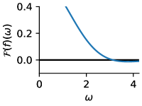
Figure 5: Fourier transform of $\tilde{k}=\frac{k}{1+k}$ when $k$ is the Gaussian kernel. The Fourier transform can be negative.

We may thus compute approximately the coefficients $\mathcal{F}[f](\bm{\omega})$ for all $\bm{\omega}\in\mathbb{R}^{d}$. In dimension $d=1$, truncating the series at $N=10^{6}$, we obtain the curve presented in Figure 5, and observe negative coefficients. To ensure that the infinite sum is negative, we now bound the residual when we truncate the sum at 2N (for $d=1$):

$$\begin{split}R_{N}(\bm{\omega})&=\sqrt{\pi}\sum_{n=2N+1}^{\infty}\frac{(-1)^{n+1}}{\sqrt{n}}e^{-\frac{||\bm{\omega}||^{2}}{2n}}\\ &=\sqrt{\pi}\sum_{n=N}^{\infty}\left[\frac{e^{-\frac{||\bm{\omega}||^{2}}{2(2n+1)}}}{\sqrt{2n+1}}-\frac{e^{-\frac{||\bm{\omega}||^{2}}{2(2n+2)}}}{\sqrt{2n+2}}\right]\\ &\leq\sqrt{\pi}\sum_{n=N}^{\infty}\left[\frac{e^{-\frac{||\bm{\omega}||^{2}}{2(2n+2)}}}{\sqrt{2n+1}}-\frac{e^{-\frac{||\bm{\omega}||^{2}}{2(2n+2)}}}{\sqrt{2n+2}}\right]\\ &\leq\sqrt{\pi}\sum_{n=N}^{\infty}\left[\frac{1}{\sqrt{2n+1}}-\frac{1}{\sqrt{2n+2}}\right]\\ &=\sqrt{\pi}\sum_{n=N}^{\infty}\frac{1}{\sqrt{2n+1}}\left[1-\sqrt{1-\frac{1}{{2n+2}}}\right]\\ &\leq\sqrt{\pi}\sum_{n=N}^{\infty}\frac{1}{\sqrt{2n+1}(2n+2)}\\ &\leq\sqrt{\frac{\pi}{8}}\sum_{n=N}^{\infty}\frac{1}{n\sqrt{n}}\\ &\leq\sqrt{\frac{\pi}{8}}\int_{N-1}^{\infty}\frac{dx}{x\sqrt{x}}\\ &=\sqrt{\frac{\pi}{2(N-1)}}.\end{split}$$

For $N=10^{6}$, this gives $R_{N}(\bm{\omega})<2\times 10^{-3}$. We observed numerically some values strictly smaller than $-2\times 10^{-3}$ for the truncation at $N=10^{6}$ of the series: in particular, $\mathcal{F}[f](2.65)=-.012$, which implies that the infinite sum is negative. We therefore conclude that $\frac{k}{k+1}$ is not positive definite when $k$ is the Gaussian kernel. Note, however, that this does not disprove the positive definiteness of $K_{\gamma}^{C}$ using the squared Euclidean cost.

B.6 Proof of Proposition 3 (stationary point using the squared Euclidean cost)

Soft-DTW divergence.

We recall that we denote $C({\bm{X}})\coloneqq C({\bm{X}},{\bm{X}})\in\mathbb{R}^{m\times m}$. Using (14), we have

$$\nabla_{\bm{X}}D_{\gamma}^{C}({\bm{X}},{\bm{Y}})=(J_{\bm{X}}C({\bm{X}},{\bm{Y}}))^{\top}\bm{E}_{\gamma}(C({\bm{X}},{\bm{Y}}))-\frac{1}{2}(J_{\bm{X}}C({\bm{X}}))^{\top}\bm{E}_{\gamma}(C({\bm{X}})).$$ (75)

Under the squared Euclidean cost, $C({\bm{X}})$ is a symmetric matrix. For any $\bm{A}\in\mathcal{A}(m,m)$, there exists $\bm{A}^{\top}\in\mathcal{A}(m,m)$. Moreover for any symmetric matrix ${\bm{C}}$, the probability $\mathbb{P}_{\gamma}(\bm{A};{\bm{C}})$ is the same as $\mathbb{P}_{\gamma}(\bm{A}^{\top};{\bm{C}})$. From (9), we therefore have that $\bm{E}_{\gamma}(C({\bm{X}}))\in\mathbb{R}^{m\times m}$ is a symmetric matrix. In order to have $\nabla_{\bm{X}}D_{\gamma}^{C}({\bm{X}},{\bm{Y}})={\bm{0}}_{m\times d}$ at ${\bm{X}}={\bm{Y}}$, it suffices that $(J_{\bm{X}}C({\bm{X}},{\bm{Y}}))^{\top}$ and $\frac{1}{2}(J_{\bm{X}}C({\bm{X}}))^{\top}$ map symmetric matrices to the same matrix. From (49), this is indeed the case for the squared Euclidean cost.

Sharp divergence.

Using (24), we get

$$\nabla_{\bm{X}}\textsc{sharp}_{\gamma}(C({\bm{X}},{\bm{Y}})) =(J_{\bm{X}}C({\bm{X}},{\bm{Y}}))^{\top}\nabla_{\bm{C}}\textsc{sharp}_{\gamma}(C({\bm{X}},{\bm{Y}}))$$ (76)

$$=(J_{\bm{X}}C({\bm{X}},{\bm{Y}}))^{\top}[\bm{E}_{\gamma}({\bm{C}})+\frac{1}{\gamma}\nabla^{2}_{\bm{C}}\textsc{sdtw}_{\gamma}(C({\bm{X}},{\bm{Y}}))C({\bm{X}},{\bm{Y}})]$$ (77)

$$=\nabla_{\bm{X}}\textsc{sdtw}_{\gamma}(C({\bm{X}},{\bm{Y}}))+\frac{1}{\gamma}(J_{\bm{X}}C({\bm{X}},{\bm{Y}}))^{\top}\nabla^{2}_{\bm{C}}\textsc{sdtw}_{\gamma}(C({\bm{X}},{\bm{Y}}))C({\bm{X}},{\bm{Y}}).$$ (78)

We therefore have

$$\nabla_{\bm{X}}S_{\gamma}^{C}({\bm{X}},{\bm{Y}})=\nabla_{\bm{X}}D_{\gamma}^{C}({\bm{X}},{\bm{Y}}) +\frac{1}{\gamma}(J_{\bm{X}}C({\bm{X}},{\bm{Y}}))^{\top}\nabla^{2}_{\bm{C}}\textsc{sdtw}_{\gamma}(C({\bm{X}},{\bm{Y}}))C({\bm{X}},{\bm{Y}})$$ (79)

$$-\frac{1}{2\gamma}(J_{\bm{X}}C({\bm{X}}))^{\top}\nabla^{2}_{\bm{C}}\textsc{sdtw}_{\gamma}(C({\bm{X}}))C({\bm{X}}).$$ (80)

From the previous paragraph, we know that $\nabla_{\bm{X}}D_{\gamma}^{C}({\bm{X}},{\bm{Y}})={\bm{0}}_{m\times d}$ at ${\bm{X}}={\bm{Y}}$ using the squared Euclidean cost. It remains to show that the sum of the other two terms in (80) is also equal to ${\bm{0}}_{m\times d}$. Since $(J_{\bm{X}}C({\bm{X}},{\bm{Y}}))^{\top}$ and $\frac{1}{2}(J_{\bm{X}}C({\bm{X}}))^{\top}$ map symmetric matrices to the same matrix using the squared Euclidean cost, it suffices to show that $\nabla^{2}_{\bm{C}}\textsc{sdtw}_{\gamma}(C({\bm{X}}))C({\bm{X}})$ is a symmetric matrix.

It is well-known that the Hessian of the log-partition under a Gibbs distribution is equal to the covariance matrix (Wainwright and Jordan, 2008). The Hessian can be seen as a $mn\times mn$ matrix. Accounting for the negative sign in (6), we have

$$\nabla_{\bm{C}}^{2}\textsc{sdtw}_{\gamma}({\bm{C}}) =-\mathbb{E}_{\gamma}[\text{vec}(A-\bm{E}_{\gamma}({\bm{C}}))\text{vec}(A-\bm{E}_{\gamma}({\bm{C}}))^{\top}]$$ (81)

$$=-\sum_{\bm{A}\in\mathcal{A}(m,n)}\mathbb{P}_{\gamma}(\bm{A};{\bm{C}})\text{vec}(\bm{A}-\bm{E}({\bm{C}}))\text{vec}(\bm{A}-\bm{E}({\bm{C}}))^{\top}$$ (82)

$$=\mathbb{E}_{\gamma}[\text{vec}(A)]\mathbb{E}_{\gamma}[\text{vec}(A)]^{\top}-\mathbb{E}_{\gamma}[\text{vec}(A)\text{vec}(A)^{\top}],$$ (83)

where $A$ is a random alignment matrix distributed according to $\mathbb{P}_{\gamma}(\bm{A};{\bm{C}})$. Equivalently, we can see the Hessian as linear map from $\mathbb{R}^{m\times n}$ to $\mathbb{R}^{m\times n}$. Applying that map to a matrix $\bm{M}\in\mathbb{R}^{m\times n}$, we obtain

$$\nabla^{2}_{\bm{C}}\textsc{sdtw}_{\gamma}({\bm{C}})\bm{M} =-\sum_{\bm{A}\in\mathcal{A}(m,n)}\mathbb{P}_{\gamma}(\bm{A};{\bm{C}})(\bm{A}-\bm{E}_{\gamma}({\bm{C}}))\langle\bm{A}-\bm{E}_{\gamma}({\bm{C}}),\bm{M}\rangle$$ (84)

$$=\langle\bm{E}_{\gamma}({\bm{C}}),\bm{M}\rangle\bm{E}_{\gamma}({\bm{C}})-\sum_{\bm{A}\in\mathcal{A}(m,n)}\mathbb{P}_{\gamma}(\bm{A};{\bm{C}})\langle\bm{A},\bm{M}\rangle\bm{A}$$ (85)

$$=\langle\bm{E}_{\gamma}({\bm{C}}),\bm{M}\rangle\bm{E}_{\gamma}({\bm{C}})-\mathbb{E}_{\gamma}[\langle A,\bm{M}\rangle A].$$ (86)

We now assume ${\bm{C}}=\bm{M}=C({\bm{X}})$. We already proved that $\bm{E}_{\gamma}({\bm{C}})$ is a symmetric matrix. Using the same argument $\mathbb{E}_{\gamma}[\langle A,\bm{M}\rangle A]$ is also symmetric. Therefore $\nabla^{2}_{\bm{C}}\textsc{sdtw}_{\gamma}({\bm{C}})\bm{M}$ is a symmetric matrix, concluding the proof.

B.7 Multiplication with the Hessian

For completeness, we also include a discussion on the multiplication with the Hessian w.r.t. ${\bm{X}}$. The product between the Hessian $\nabla^{2}_{\bm{X}}\textsc{sdtw}_{\gamma}(C({\bm{X}},{\bm{Y}}))$ and any ${\bm{Z}}\in\mathbb{R}^{m\times d}$ is equal to the product between the Jacobian of $\nabla_{\bm{X}}\textsc{sdtw}_{\gamma}(C({\bm{X}},{\bm{Y}}))$ and ${\bm{Z}}$:

$$\nabla^{2}_{\bm{X}}\textsc{sdtw}_{\gamma}(C({\bm{X}},{\bm{Y}})){\bm{Z}}=J_{\bm{X}}[\nabla_{\bm{X}}\textsc{sdtw}_{\gamma}(C({\bm{X}},{\bm{Y}}))]{\bm{Z}}=J_{\bm{X}}[J_{\bm{X}}C({\bm{X}},{\bm{Y}})^{\top}\bm{E}_{\gamma}(C({\bm{X}},{\bm{Y}}))]{\bm{Z}}.$$ (87)

Using the product rule and the chain rule, we obtain

$$\nabla^{2}_{\bm{X}}\textsc{sdtw}_{\gamma}(C({\bm{X}},{\bm{Y}})){\bm{Z}}=\underbrace{[J_{\bm{X}}(J_{\bm{X}}C({\bm{X}},{\bm{Y}}))^{\top}\bm{E}_{\gamma}(C({\bm{X}},{\bm{Y}}))]}_{\bm{B}_{\gamma}({\bm{X}},{\bm{Y}})}{\bm{Z}}+(J_{\bm{X}}C({\bm{X}},{\bm{Y}}))^{\top}\nabla^{2}_{\bm{C}}\textsc{sdtw}_{\gamma}(C({\bm{X}},{\bm{Y}}))J_{\bm{X}}C({\bm{X}},{\bm{Y}}){\bm{Z}}.$$ (88)

Similarly,

$$\nabla^{2}_{\bm{X}}\textsc{sdtw}_{\gamma}(C({\bm{X}})){\bm{Z}}=\underbrace{[J_{\bm{X}}(J_{\bm{X}}C({\bm{X}}))^{\top}\bm{E}_{\gamma}(C({\bm{X}}))]}_{\bm{B}_{\gamma}({\bm{X}})}{\bm{Z}}+(J_{\bm{X}}C({\bm{X}}))^{\top}\nabla^{2}_{\bm{C}}\textsc{sdtw}_{\gamma}(C({\bm{X}}))J_{\bm{X}}C({\bm{X}}){\bm{Z}}.$$ (89)

From now on, we assume the squared Euclidean cost. Using (45), we obtain

$$[\bm{B}_{\gamma}({\bm{X}},{\bm{Y}}){\bm{Z}}]_{i,k}=\sum_{j=1}^{n}[\bm{E}_{\gamma}(C({\bm{X}},{\bm{Y}}))]_{i,j}z_{i,k}\quad i\in[m],k\in[d]$$ (90)

or equivalently

$$\bm{B}_{\gamma}({\bm{X}},{\bm{Y}}){\bm{Z}}={\bm{Z}}\circ(\bm{E}_{\gamma}(C({\bm{X}},{\bm{Y}})){\bm{1}}_{n\times d})\in\mathbb{R}^{m\times d}.$$ (91)

Similarly, using (47) and the fact that $\bm{E}_{\gamma}(C({\bm{X}}))$ is a symmetric matrix, we obtain

$$[\bm{B}_{\gamma}({\bm{X}}){\bm{Z}}]_{i,k}=2\sum_{j=1}^{n}[\bm{E}_{\gamma}(C({\bm{X}}))]_{i,j}(z_{i,k}-z_{j,k})$$ (92)

or equivalently

$$\bm{B}_{\gamma}({\bm{X}}){\bm{Z}}=2{\bm{Z}}\circ(\bm{E}_{\gamma}(C({\bm{X}}){\bm{1}}_{m\times d})-2\bm{E}_{\gamma}(C({\bm{X}})){\bm{Z}}\in\mathbb{R}^{m\times d}.$$ (93)

At ${\bm{X}}={\bm{Y}}$, we therefore get

$$\bm{B}_{\gamma}({\bm{X}},{\bm{Y}}){\bm{Z}}-\frac{1}{2}\bm{B}_{\gamma}({\bm{X}}){\bm{Z}}=\bm{E}_{\gamma}(C({\bm{X}}))^{\top}{\bm{Z}}=\bm{E}_{\gamma}(C({\bm{X}})){\bm{Z}}.$$ (94)

At ${\bm{X}}={\bm{Y}}$, from (49) and (54), we also have

$$(J_{\bm{X}}C({\bm{X}}))^{\top}\nabla^{2}_{\bm{C}}\bm{E}_{\gamma}(C({\bm{X}}))J_{\bm{X}}C({\bm{X}}){\bm{Z}}=2J_{\bm{X}}C({\bm{X}},{\bm{X}})^{\top}\nabla^{2}_{\bm{C}}\textsc{sdtw}_{\gamma}(C({\bm{X}}))(J_{\bm{X}}C({\bm{X}},{\bm{X}}){\bm{Z}}+(J_{\bm{X}}C({\bm{X}},{\bm{X}}){\bm{Z}})^{\top}).$$ (95)

Putting everything together, at ${\bm{X}}={\bm{Y}}$, we have

$$\nabla^{2}_{\bm{X}}D_{\gamma}^{C}({\bm{X}},{\bm{Y}}){\bm{Z}} =\nabla^{2}_{\bm{X}}\textsc{sdtw}_{\gamma}(C({\bm{X}},{\bm{Y}})){\bm{Z}}-\frac{1}{2}\nabla^{2}_{\bm{X}}\textsc{sdtw}_{\gamma}(C({\bm{X}})){\bm{Z}}$$ (96)

$$=\bm{E}_{\gamma}(C({\bm{X}})){\bm{Z}}-J_{\bm{X}}C({\bm{X}},{\bm{X}})^{\top}\nabla^{2}_{\bm{C}}\textsc{sdtw}_{\gamma}(C({\bm{X}}))(J_{\bm{X}}C({\bm{X}},{\bm{X}}){\bm{Z}})^{\top}.$$ (97)

An open question is to prove that ${\bm{X}}={\bm{Y}}$ is a local minimum, i.e., $\langle Z,\nabla^{2}_{\bm{X}}D_{\gamma}^{C}({\bm{X}},{\bm{Y}}){\bm{Z}}\rangle>0$ for all ${\bm{Z}}\in\mathbb{R}^{m\times d}$.

B.8 Proof of Proposition 35 (limits w.r.t. $\gamma$)

Limit to zero.

Since both $\textsc{sdtw}_{\gamma}({\bm{C}})$ and $\textsc{sharp}_{\gamma}({\bm{C}})$ converge to $\textsc{dtw}({\bm{C}})$ when $\gamma\to 0$, both $D_{\gamma}^{C}({\bm{X}},{\bm{Y}})$ and $S_{\gamma}^{C}({\bm{X}},{\bm{Y}})$ converge to

$$\textsc{dtw}(C({\bm{X}},{\bm{Y}}))-\frac{1}{2}\textsc{dtw}(C({\bm{X}},{\bm{X}}))-\frac{1}{2}\textsc{dtw}(C({\bm{Y}},{\bm{Y}})).$$ (98)

Since the optimal alignment of $\bm{A}^{\star}({\bm{C}}({\bm{X}},{\bm{X}}))$ is the identity matrix under assumption A.2, we have $\textsc{dtw}(C({\bm{X}},{\bm{X}}))=0$ and similarly $\textsc{dtw}(C({\bm{Y}},{\bm{Y}}))=0$. Therefore, both $D_{\gamma}^{C}({\bm{X}},{\bm{Y}})$ and $S_{\gamma}^{C}({\bm{X}},{\bm{Y}})$ converge to $\textsc{dtw}(C({\bm{X}},{\bm{Y}}))$.

Limit to infinity.

From (11), when $\gamma\to\infty$, the solution becomes the maximum entropy one, $\bm{p}^{\star}={\bm{1}}/|\mathcal{A}(m,n)|$. Hence, $\langle\bm{p}^{\star},s({\bm{C}})\rangle$ converge to the mean cost (29). This gives the limit for the $S_{\gamma}^{C}$ case. For the $D_{\gamma}^{C}$ case, we also need to take into account the entropy terms

$$-\gamma H(\bm{p}_{\gamma}(C({\bm{X}},{\bm{Y}}))+\frac{\gamma}{2}H(\bm{p}_{\gamma}(C({\bm{X}},{\bm{X}})))+\frac{\gamma}{2}H(\bm{p}_{\gamma}(C({\bm{Y}},{\bm{Y}}))).$$ (99)

When $\gamma\to\infty$, each term attains the maximum entropy value and we get

$$-\gamma\log|\mathcal{A}(m,n)|+\frac{\gamma}{2}\log|\mathcal{A}(m,m)|+\frac{\gamma}{2}\log|\mathcal{A}(n,n)|=\frac{\gamma}{2}\log\frac{|\mathcal{A}(m,m)||\mathcal{A}(n,n)|}{|\mathcal{A}(m,n)|^{2}}\,.$$ (100)

When $m=n$, the terms cancel out. Hence, $D_{\gamma}^{C}({\bm{X}},{\bm{Y}})$ converge. When, $m\neq n$, the positive terms are stronger, and the limit goes to $\infty$. By definition, we have

$$\begin{split}D_{\gamma}^{C}({\bm{X}},{\bm{Y}})&=\textsc{sdtw}_{\gamma}(C({\bm{X}},{\bm{Y}}))-\frac{1}{2}\textsc{sdtw}_{\gamma}(C({\bm{X}},{\bm{X}}))-\frac{1}{2}\textsc{sdtw}_{\gamma}(C({\bm{Y}},{\bm{Y}}))\\ &=-\gamma\log\sum_{\bm{A}\in\mathcal{A}(m,n)}\exp(-\langle\bm{A},C({\bm{X}},{\bm{Y}})\rangle/\gamma)\\ &\quad\quad+\frac{\gamma}{2}\log\sum_{\bm{A}\in\mathcal{A}(m,m)}\exp(-\langle\bm{A},C({\bm{X}},{\bm{X}})\rangle/\gamma)+\frac{\gamma}{2}\log\sum_{\bm{A}\in\mathcal{A}(n,n)}\exp(-\langle\bm{A},C({\bm{Y}},{\bm{Y}})\rangle/\gamma)\\ &=-\frac{\gamma}{2}\log\frac{|\mathcal{A}(m,n)|^{2}}{|\mathcal{A}(m,m)||\mathcal{A}(n,n)|}-\gamma\log\left[\frac{1}{|\mathcal{A}(m,n)|}\sum_{\bm{A}\in\mathcal{A}(m,n)}\exp(-\langle\bm{A},C({\bm{X}},{\bm{Y}})\rangle/\gamma)\right]\\ &\quad\quad+\frac{\gamma}{2}\log\left[\frac{1}{|\mathcal{A}(m,m)|}\sum_{\bm{A}\in\mathcal{A}(m,m)}\exp(-\langle\bm{A},C({\bm{X}},{\bm{X}})\rangle/\gamma)\right]\\ &\quad\quad+\frac{\gamma}{2}\log\left[\frac{1}{|\mathcal{A}(n,n)|}\sum_{\bm{A}\in\mathcal{A}(n,n)}\exp(-\langle\bm{A},C({\bm{Y}},{\bm{Y}})\rangle/\gamma)\right]\end{split}$$ (101)

Let us first consider the limit of the second term in this sum when $\gamma\rightarrow+\infty$:

$$\begin{split}\gamma\log\left[\frac{1}{|\mathcal{A}(m,n)|}\sum_{\bm{A}\in\mathcal{A}(m,n)}\exp(-\langle\bm{A},C({\bm{X}},{\bm{Y}})\rangle/\gamma)\right]&=\gamma\log\left[\frac{1}{|\mathcal{A}(m,n)|}\sum_{\bm{A}\in\mathcal{A}(m,n)}\left(1-\frac{\langle\bm{A},C({\bm{X}},{\bm{Y}})\rangle}{\gamma}+o(1/\gamma)\right)\right]\\ &=\gamma\log\left[1-\frac{\text{{mean\_cost}}(C({\bm{X}},{\bm{Y}}))}{\gamma}+o(1/\gamma)\right]\\ &=-\text{{mean\_cost}}(C({\bm{X}},{\bm{Y}}))+o(1)\,.\end{split}$$

A similar computation for the third and fourth term in (101) leads to

$$\begin{split}D_{\gamma}^{C}({\bm{X}},{\bm{Y}})&=-\frac{\gamma}{2}\log\frac{|\mathcal{A}(m,n)|^{2}}{|\mathcal{A}(m,m)||\mathcal{A}(n,n)|}+\text{{mean\_cost}}(C({\bm{X}},{\bm{Y}}))-\frac{1}{2}\text{{mean\_cost}}(C({\bm{X}},{\bm{X}}))\\ &~{}~{}~{}-\frac{1}{2}\text{{mean\_cost}}(C({\bm{Y}},{\bm{Y}}))+o(1)\\ &=-\frac{\gamma}{2}\log\frac{|\mathcal{A}(m,n)|^{2}}{|\mathcal{A}(m,m)||\mathcal{A}(n,n)|}+M^{C}({\bm{X}},{\bm{Y}})+o(1)\,.\end{split}$$

When $m=n$, the first term is equal to $0$, so we get $\lim_{\gamma\rightarrow+\infty}D_{\gamma}^{C}({\bm{X}},{\bm{Y}})=M^{C}({\bm{X}},{\bm{Y}})$. When $m\neq n$, on the other hand, we can use the fact that for any integers $m,n$:

$$|\mathcal{A}(m,n)|=\text{{Delannoy}}(m-1,n-1)\,,$$

where $\text{{Delannoy}}(m,n)$ is the Delannoy number, i.e., the number of paths on a rectangular grid from the origin $(0,0)$ to the northeast corner $(m,n)$, using only single steps north, east or northeast (the $(m-1,n-1)$ term stems from the fact that alignment matrices represent paths starting from $(1,1)$ and not $(0,0)$). We can now use Lemma B.8 below to get, when $m\neq n$:

$$\log\frac{|\mathcal{A}(m,n)|^{2}}{|\mathcal{A}(m,m)||\mathcal{A}(n,n)|}=\log\frac{\text{{Delannoy}}(m-1,n-1)^{2}}{\text{{Delannoy}}(m-1,m-1)\times\text{{Delannoy}}(n-1,n-1)}<0\,,$$

and therefore that $\lim_{\gamma\rightarrow+\infty}D_{\gamma}^{C}({\bm{X}},{\bm{Y}})=+\infty$.

For any $m,n\in\mathbb{N}$, if $m\neq n$ then

$$\log\frac{\text{{Delannoy}}(m,n)^{2}}{\text{{Delannoy}}(m,m)\times\text{{Delannoy}}(n,n)}<0\,.$$

Proof.

We use the following characterization of Delannoy numbers (e.g., Banderier and Schwer, 2005):

$$\text{{Delannoy}}(m,n)=\sum_{k=0}^{\min(m,n)}\left(\begin{array}[]{c}m\\ k\end{array}\right)\left(\begin{array}[]{c}n\\ k\end{array}\right)2^{k}\,,$$

to obtain, assuming without loss of generality that $m<n$:

$$\begin{split}\text{{Delannoy}}(m,n)^{2}&=\left[\sum_{k=0}^{m}\left(\begin{array}[]{c}m\\ k\end{array}\right)\left(\begin{array}[]{c}n\\ k\end{array}\right)2^{k}\right]^{2}\\ &\leq\left[\sum_{k=0}^{m}\left(\begin{array}[]{c}m\\ k\end{array}\right)^{2}2^{k}\right]\times\left[\sum_{k=0}^{m}\left(\begin{array}[]{c}n\\ k\end{array}\right)^{2}2^{k}\right]\\ &<\left[\sum_{k=0}^{m}\left(\begin{array}[]{c}m\\ k\end{array}\right)^{2}2^{k}\right]\times\left[\sum_{k=0}^{n}\left(\begin{array}[]{c}n\\ k\end{array}\right)^{2}2^{k}\right]\\ &=\text{{Delannoy}}(m,m)\times\text{{Delannoy}}(n,n)\,,\end{split}$$

where we used Cauchy-Schwartz inequality for the first inequality, and the fact that $m<n$ for the second (strict) inequality. ∎

Appendix C Additional empirical results

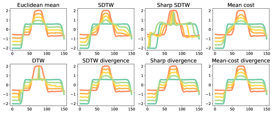
Figure 6: Interpolation between two time series, from the GunPoint dataset.

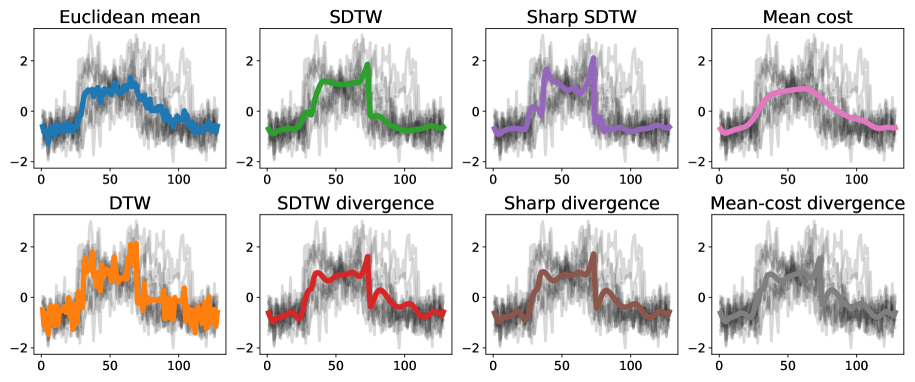
Figure 7: Barycenters on the CBF dataset.

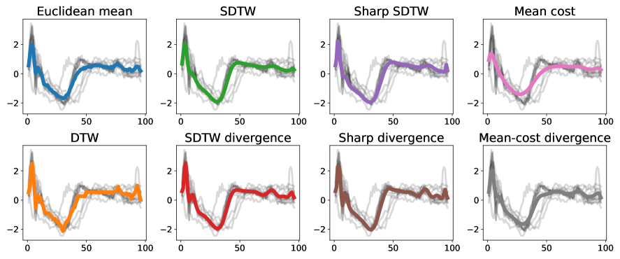
Figure 8: Barycenters on the ECG200 dataset.

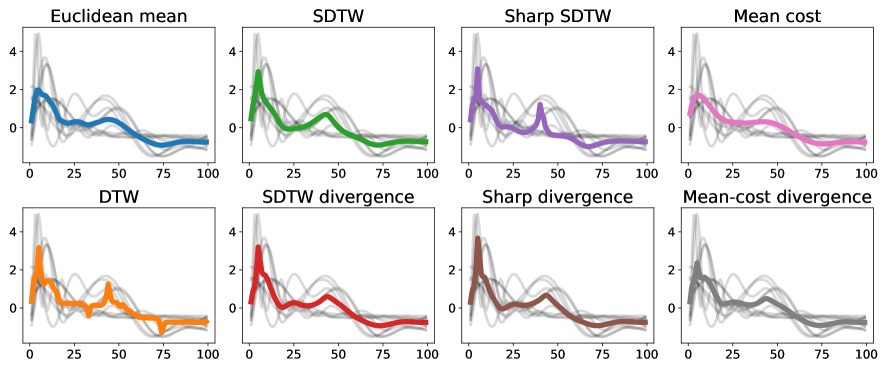
Figure 9: Barycenters on the Medical Images dataset.

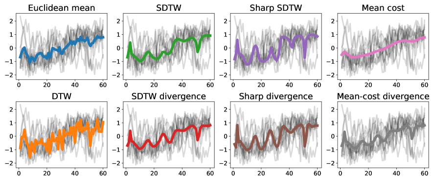
Figure 10: Barycenters on the synthetic control dataset.

Table 4: Three nearest neighbors results. Each number indicates the percentage of datasets in the UCR archive for which using $A$ in the nearest neighbor classifier is within $99\%$ or better than using $B$ .

$A$ ($\downarrow$) vs. $B$ ($\rightarrow$)	Euc.	DTW	SDTW	SDTW div	Sharp	Sharp div	Mean cost	Mean-cost div
Euc.	-	39.29	29.49	31.17	37.18	28.00	95.24	65.48
DTW	70.24	-	53.85	45.45	57.69	42.67	90.48	83.33
SDTW	82.05	88.46	-	66.23	83.33	58.67	98.72	89.74
SDTW div	90.91	84.42	85.71	-	83.12	70.67	98.70	94.81
Sharp	78.21	82.05	64.10	58.44	-	53.33	98.72	87.18
Sharp div	86.67	90.67	81.33	77.33	89.33	-	98.67	96.00
Mean cost	8.33	13.10	6.41	3.90	5.13	4.00	-	44.05
Mean-cost div	46.43	34.52	24.36	20.78	24.36	21.33	98.81	-

Table 5: Five nearest neighbor results. Each number indicates the percentage of datasets in the UCR archive for which using $A$ in the nearest neighbor classifier is within $99\%$ or better than using $B$ .

$A$ ($\downarrow$) vs. $B$ ($\rightarrow$)	Euc.	DTW	SDTW	SDTW div	Sharp	Sharp div	Mean cost	Mean-cost div
Euc.	-	40.48	30.77	28.57	33.33	24.68	95.29	70.24
DTW	73.81	-	48.72	44.16	55.13	45.45	88.10	83.33
SDTW	85.90	84.62	-	61.04	74.36	63.64	94.87	82.05
SDTW div	84.42	88.31	81.82	-	81.82	74.03	96.10	85.71
Sharp	85.90	87.18	70.51	58.44	-	59.74	97.44	82.05
Sharp div	90.91	84.42	80.52	76.62	84.42	-	96.10	87.01
Mean cost	10.59	13.10	10.26	7.79	7.69	7.79	-	45.24
Mean-cost div	45.24	32.14	26.92	20.78	26.92	19.48	98.81	-

Table 6: Nearest neighbor classification accuracy with $k=1$.

Dataset name	Euc.	DTW	SDTW	SDTW div	Sharp	Sharp div	Mean cost	Mean-cost div
50words	63.08	69.01	80.66	81.54	79.12	79.78	58.90	67.91
Adiac	61.13	60.36	61.38	71.36	60.10	72.12	28.39	54.48
ArrowHead	80.00	70.29	77.14	81.71	80.57	79.43	72.57	78.86
Beef	66.67	63.33	63.33	63.33	63.33	63.33	20.00	20.00
BeetleFly	75.00	70.00	70.00	70.00	70.00	75.00	50.00	50.00
BirdChicken	55.00	75.00	75.00	75.00	75.00	75.00	50.00	50.00
CBF	85.22	99.67	99.67	99.67	99.67	99.67	78.78	95.00
Car	73.33	73.33	73.33	75.00	75.00	78.33	23.33	23.33
ChlorineConcentration	65.00	64.84	62.29	64.84	65.05	65.65	38.20	55.44
CinC_ECG_torso	89.71	65.07	93.41	93.55	92.54	93.84	25.36	25.36
Coffee	100.00	100.00	100.00	100.00	100.00	100.00	53.57	96.43
Computers	57.60	70.00	69.60	70.00	69.20	67.20	50.00	50.00
Cricket_X	57.69	75.38	77.69	80.00	77.95	79.23	42.56	61.54
Cricket_Y	56.67	74.36	76.67	78.72	74.36	77.18	47.95	61.28
Cricket_Z	58.72	75.38	77.69	80.26	77.69	79.74	43.08	63.33
DiatomSizeReduction	93.46	96.73	92.16	94.44	92.81	93.46	92.16	93.46
DistalPhalanxOutlineAgeGroup	78.25	79.25	79.25	79.75	79.50	80.50	59.50	76.75
DistalPhalanxOutlineCorrect	75.17	76.83	79.00	76.83	76.83	75.17	36.83	71.33
DistalPhalanxTW	72.75	70.75	73.25	72.25	74.50	72.50	51.00	71.00
ECG200	88.00	77.00	86.00	88.00	82.00	87.00	87.00	88.00
ECG5000	92.49	92.44	93.07	92.36	92.78	92.47	91.80	92.38
ECGFiveDays	79.67	76.77	61.67	93.50	62.49	91.17	61.44	83.86
Earthquakes	67.39	74.22	82.61	74.53	82.61	74.22	81.99	81.99
ElectricDevices	54.93	60.02	NA	NA	NA	NA	26.17	59.12
FISH	78.29	82.29	92.00	92.57	90.29	91.43	12.57	12.57
FaceAll	71.36	80.77	74.38	82.31	76.27	82.78	25.33	81.89
FaceFour	78.41	82.95	82.95	89.77	87.50	89.77	62.50	84.09
FacesUCR	76.93	90.49	92.34	94.78	92.34	94.54	45.90	80.44
FordA	65.90	56.21	NA	NA	NA	NA	51.26	51.26
FordB	55.78	59.41	58.55	NA	58.83	NA	48.84	48.84
Gun_Point	91.33	90.67	97.33	98.00	98.00	98.00	82.00	90.00
Ham	60.00	46.67	49.52	58.10	58.10	61.90	48.57	48.57
HandOutlines	80.10	79.80	NA	NA	NA	NA	63.80	63.80
Haptics	37.01	37.66	39.94	39.94	40.26	41.56	21.75	21.75
Herring	51.56	53.12	57.81	57.81	60.94	62.50	59.38	59.38
InlineSkate	34.18	38.36	42.55	43.09	42.00	42.36	15.64	15.64
InsectWingbeatSound	56.16	35.51	55.05	56.87	56.26	57.07	54.55	56.97
ItalyPowerDemand	95.53	95.04	93.68	95.04	94.07	95.43	90.38	94.95
LargeKitchenAppliances	49.33	79.47	79.73	79.73	79.73	79.73	33.33	33.33
Lighting2	75.41	86.89	90.16	88.52	90.16	86.89	54.10	54.10
Lighting7	57.53	72.60	73.97	78.08	75.34	82.19	57.53	68.49
MALLAT	91.43	93.39	89.72	91.39	90.62	92.24	12.54	12.54
Meat	93.33	93.33	95.00	93.33	95.00	93.33	33.33	33.33
MedicalImages	68.42	73.68	74.61	75.92	76.18	77.76	57.89	69.61
MiddlePhalanxOutlineAgeGroup	74.00	75.00	71.00	73.25	75.25	73.75	66.25	73.25
MiddlePhalanxOutlineCorrect	75.33	64.83	72.67	76.33	66.83	71.83	35.33	70.67
MiddlePhalanxTW	56.14	58.40	58.40	58.40	58.40	58.40	52.63	59.15
MoteStrain	87.86	83.47	90.18	89.86	91.53	87.62	88.18	80.35
NonInvasiveFatalECG_Thorax1	82.90	78.98	NA	NA	NA	NA	2.44	2.44
NonInvasiveFatalECG_Thorax2	87.99	86.46	NA	NA	NA	NA	2.44	2.44
OSULeaf	52.07	59.09	70.25	69.83	70.25	69.83	9.50	9.50
OliveOil	86.67	83.33	86.67	86.67	86.67	86.67	16.67	16.67
PhalangesOutlinesCorrect	76.11	72.61	74.59	77.04	71.91	77.39	42.31	73.08
Phoneme	10.92	22.84	24.00	22.73	21.89	23.26	2.00	2.00
Plane	96.19	100.00	100.00	100.00	100.00	100.00	84.76	96.19
ProximalPhalanxOutlineAgeGroup	78.54	80.49	75.12	80.98	80.98	80.98	46.34	76.59
ProximalPhalanxOutlineCorrect	80.76	77.66	79.04	83.51	74.23	83.51	31.96	73.20
ProximalPhalanxTW	70.75	74.00	74.75	70.25	75.00	73.25	45.25	70.25
RefrigerationDevices	39.47	46.40	45.87	44.80	45.60	NA	33.33	33.33
ScreenType	36.00	40.00	41.33	40.27	39.47	39.47	33.33	33.33
ShapeletSim	53.89	65.00	58.33	87.22	64.44	82.78	50.00	50.00
ShapesAll	75.17	76.83	83.67	84.33	80.83	82.17	1.67	1.67
SmallKitchenAppliances	34.40	64.27	66.67	66.67	67.47	65.87	33.33	33.33
SonyAIBORobotSurface	69.55	72.55	72.55	76.71	72.55	76.54	45.42	76.04
SonyAIBORobotSurfaceII	85.94	83.11	84.26	84.89	83.11	83.95	76.39	84.05
StarLightCurves	84.88	NA	NA	NA	NA	NA	57.72	NA
Strawberry	93.80	93.96	93.96	93.80	93.80	93.64	79.45	93.80
SwedishLeaf	78.88	79.20	82.40	88.16	82.24	89.12	46.72	79.84
Symbols	89.95	94.97	96.18	95.38	95.18	95.28	86.93	90.15
ToeSegmentation1	67.98	77.19	83.33	82.89	80.26	81.58	63.16	63.16
ToeSegmentation2	80.77	83.85	90.77	86.15	92.31	92.31	79.23	83.85
Trace	76.00	100.00	100.00	100.00	100.00	100.00	47.00	72.00
TwoLeadECG	74.71	90.52	90.52	90.43	89.73	88.59	57.77	70.15
Two_Patterns	90.68	100.00	100.00	100.00	100.00	100.00	94.78	96.72
UWaveGestureLibraryAll	94.81	89.17	NA	NA	NA	NA	12.53	12.53
Wine	61.11	57.41	55.56	62.96	55.56	62.96	50.00	61.11
WordsSynonyms	61.76	64.89	76.80	78.06	74.92	76.49	55.33	65.20
Worms	36.46	46.41	47.51	48.07	49.17	42.54	41.99	41.99
WormsTwoClass	58.56	66.30	55.80	67.40	57.46	64.09	41.99	41.99
synthetic_control	88.00	99.33	97.67	99.33	99.33	99.33	76.67	98.67
uWaveGestureLibrary_X	73.93	72.75	78.48	78.73	77.58	78.00	72.84	74.37
uWaveGestureLibrary_Y	66.16	63.40	70.30	NA	69.82	71.13	64.43	67.42
uWaveGestureLibrary_Z	64.96	65.83	68.51	69.65	68.06	68.90	62.90	64.91
wafer	99.55	97.99	99.30	99.56	99.43	99.59	99.25	99.51
yoga	83.03	83.67	83.97	85.30	84.70	83.57	46.43	46.43

Table 7: Nearest neighbor classification accuracy with $k=3$.

Dataset name	Euc.	DTW	SDTW	SDTW div	Sharp	Sharp div	Mean cost	Mean-cost div
50words	61.98	66.37	80.22	80.66	77.80	78.90	59.34	66.81
Adiac	55.24	57.29	56.78	69.05	54.99	66.50	26.34	49.10
ArrowHead	79.43	70.86	80.57	79.43	78.86	82.86	72.57	84.57
Beef	60.00	56.67	53.33	56.67	56.67	56.67	20.00	20.00
BeetleFly	65.00	70.00	50.00	65.00	75.00	75.00	50.00	50.00
BirdChicken	45.00	60.00	60.00	60.00	60.00	60.00	50.00	50.00
CBF	83.78	99.67	99.67	99.67	99.67	99.67	82.56	89.78
Car	66.67	55.00	61.67	66.67	56.67	56.67	23.33	23.33
ChlorineConcentration	56.59	56.69	56.12	56.54	56.69	56.69	38.44	51.54
CinC_ECG_torso	85.22	49.78	86.67	86.67	85.87	85.58	24.78	24.78
Coffee	100.00	92.86	92.86	92.86	92.86	92.86	53.57	92.86
Computers	62.00	71.20	71.20	71.20	71.20	71.20	50.00	50.00
Cricket_X	51.79	74.36	75.38	77.44	72.56	75.13	42.05	55.38
Cricket_Y	50.51	70.51	71.03	76.41	71.03	73.33	44.62	56.92
Cricket_Z	54.62	75.38	77.95	78.72	76.92	78.97	42.31	59.23
DiatomSizeReduction	89.22	92.81	89.22	89.87	89.87	89.87	87.58	89.54
DistalPhalanxOutlineAgeGroup	78.50	83.50	83.75	79.75	83.25	79.25	59.25	79.25
DistalPhalanxOutlineCorrect	75.83	79.83	79.33	79.83	79.83	80.67	36.67	74.33
DistalPhalanxTW	75.75	73.00	72.75	75.00	75.00	76.75	53.75	72.75
ECG200	90.00	80.00	88.00	89.00	88.00	89.00	86.00	88.00
ECG5000	93.49	93.98	94.00	94.16	93.98	94.20	93.44	93.47
ECGFiveDays	73.98	62.02	67.25	82.00	66.32	82.81	52.50	80.02
Earthquakes	74.22	78.88	78.88	78.88	78.88	78.88	81.99	81.99
ElectricDevices	56.40	61.08	NA	NA	NA	NA	25.77	60.42
FISH	75.43	79.43	90.29	90.29	90.29	91.43	12.57	12.57
FaceAll	67.22	80.77	79.94	83.37	75.09	84.97	28.46	80.53
FaceFour	65.91	68.18	68.18	72.73	59.09	77.27	46.59	69.32
FacesUCR	67.76	88.63	90.44	93.90	91.32	93.41	47.17	71.32
FordA	67.15	57.46	NA	NA	NA	NA	51.26	51.26
FordB	58.33	61.83	61.94	NA	61.83	NA	51.16	51.16
Gun_Point	87.33	88.67	97.33	98.00	98.00	98.00	84.67	84.67
Ham	59.05	51.43	52.38	62.86	57.14	61.90	51.43	51.43
HandOutlines	84.90	81.00	NA	NA	NA	NA	63.80	63.80
Haptics	38.64	42.86	41.23	41.56	37.01	43.51	21.75	21.75
Herring	56.25	48.44	64.06	60.94	62.50	65.62	59.38	59.38
InlineSkate	23.82	35.64	37.45	37.64	35.82	35.45	15.64	15.64
InsectWingbeatSound	59.24	36.21	56.67	58.18	57.22	58.33	57.07	58.28
ItalyPowerDemand	95.63	94.56	94.95	95.14	94.56	95.04	89.60	94.95
LargeKitchenAppliances	45.60	80.00	80.00	77.60	80.00	77.07	33.33	33.33
Lighting2	77.05	86.89	91.80	90.16	83.61	85.25	45.90	45.90
Lighting7	60.27	71.23	79.45	82.19	78.08	82.19	57.53	71.23
MALLAT	91.98	92.84	92.54	92.88	92.15	92.75	12.45	12.45
Meat	93.33	93.33	93.33	93.33	93.33	91.67	33.33	33.33
MedicalImages	67.76	70.92	72.11	73.42	72.76	74.61	57.24	69.21
MiddlePhalanxOutlineAgeGroup	73.50	76.00	76.00	74.50	76.00	76.00	67.75	74.50
MiddlePhalanxOutlineCorrect	77.17	72.17	74.50	77.67	73.67	76.00	35.50	75.33
MiddlePhalanxTW	58.40	61.15	60.65	61.15	61.65	62.16	51.88	58.65
MoteStrain	86.18	81.39	88.18	87.46	89.54	87.86	85.14	83.87
NonInvasiveFatalECG_Thorax1	82.54	78.63	NA	NA	NA	NA	2.54	2.54
NonInvasiveFatalECG_Thorax2	88.40	86.31	NA	NA	NA	NA	2.54	2.54
OSULeaf	50.41	57.44	59.50	61.98	64.88	65.29	19.01	19.01
OliveOil	90.00	86.67	86.67	86.67	86.67	86.67	40.00	40.00
PhalangesOutlinesCorrect	77.97	75.41	76.57	79.37	76.57	79.14	42.07	73.66
Phoneme	10.34	23.95	21.99	23.58	23.10	25.05	7.07	7.07
Plane	96.19	100.00	100.00	100.00	100.00	100.00	84.76	96.19
ProximalPhalanxOutlineAgeGroup	81.95	80.98	81.46	80.98	81.95	81.95	48.78	80.49
ProximalPhalanxOutlineCorrect	84.88	83.16	81.79	85.57	78.01	84.19	31.62	74.91
ProximalPhalanxTW	77.00	79.00	78.50	77.50	77.25	78.75	45.50	78.00
RefrigerationDevices	39.20	46.40	46.13	45.87	46.67	46.13	33.33	33.33
ScreenType	38.40	39.20	42.13	36.53	39.20	37.07	33.33	33.33
ShapeletSim	52.78	62.78	62.78	80.00	68.33	81.67	50.00	50.00
ShapesAll	69.00	71.00	77.33	77.67	75.67	NA	1.67	1.67
SmallKitchenAppliances	36.53	67.47	70.67	70.67	67.73	67.20	33.33	33.33
SonyAIBORobotSurface	57.40	61.73	61.73	61.73	61.73	61.73	43.59	67.22
SonyAIBORobotSurfaceII	79.85	80.27	77.65	79.12	79.01	80.90	76.50	80.06
StarLightCurves	84.82	NA	NA	NA	NA	NA	NA	NA
Strawberry	92.33	91.84	91.68	92.01	90.05	91.03	78.96	90.38
SwedishLeaf	71.84	77.92	80.48	86.56	78.88	87.36	47.84	77.44
Symbols	85.03	92.86	96.18	96.18	95.98	96.08	81.91	86.13
ToeSegmentation1	60.53	75.44	82.02	77.63	75.88	78.51	57.46	63.60
ToeSegmentation2	82.31	81.54	89.23	89.23	91.54	93.08	82.31	86.15
Trace	65.00	100.00	100.00	100.00	100.00	100.00	47.00	64.00
TwoLeadECG	63.48	85.16	85.34	63.48	82.44	63.74	55.66	63.21
Two_Patterns	85.95	100.00	100.00	100.00	100.00	100.00	90.72	94.20
UWaveGestureLibraryAll	94.39	89.53	NA	NA	NA	NA	12.62	12.62
Wine	55.56	57.41	62.96	62.96	51.85	61.11	50.00	61.11
WordsSynonyms	56.74	59.56	72.41	69.59	70.85	72.10	54.23	59.56
Worms	36.46	42.54	42.54	42.54	42.54	42.54	13.81	13.81
WormsTwoClass	59.12	64.09	70.17	70.17	65.19	65.19	58.01	58.01
synthetic_control	91.00	98.33	98.33	98.33	98.33	98.33	74.67	98.67
uWaveGestureLibrary_X	73.03	73.73	78.00	78.31	76.97	77.41	71.94	73.84
uWaveGestureLibrary_Y	66.67	63.18	70.63	71.36	70.18	NA	65.47	67.17
uWaveGestureLibrary_Z	65.75	66.78	68.37	69.43	67.87	68.87	64.38	66.50
wafer	99.38	97.52	99.06	99.42	99.06	99.45	99.06	99.45
yoga	79.23	82.17	82.53	82.33	82.23	82.33	46.43	46.43

Table 8: Nearest neighbor classification accuracy with $k=5$.

Dataset name	Euc.	DTW	SDTW	SDTW div	Sharp	Sharp div	Mean cost	Mean-cost div
50words	61.98	66.15	77.80	79.12	75.60	77.80	57.80	65.93
Adiac	52.17	53.20	59.34	63.68	55.75	61.64	25.06	46.55
ArrowHead	66.86	68.57	62.86	64.57	63.43	66.86	62.29	68.57
Beef	50.00	43.33	46.67	43.33	43.33	43.33	20.00	20.00
BeetleFly	60.00	70.00	60.00	65.00	70.00	80.00	50.00	50.00
BirdChicken	55.00	65.00	70.00	75.00	65.00	60.00	50.00	50.00
CBF	76.67	98.22	98.22	98.22	98.22	98.22	75.56	88.78
Car	63.33	50.00	66.67	66.67	63.33	66.67	31.67	31.67
ChlorineConcentration	54.87	54.82	54.87	54.87	54.82	54.66	44.32	51.46
CinC_ECG_torso	77.39	42.61	80.14	80.22	82.46	83.26	24.78	24.78
Coffee	96.43	96.43	96.43	96.43	96.43	96.43	60.71	96.43
Computers	60.40	68.80	69.60	68.40	69.60	68.00	50.00	50.00
Cricket_X	48.21	72.56	71.79	71.79	71.54	72.82	40.77	57.18
Cricket_Y	50.26	68.46	68.46	71.79	68.72	73.85	42.82	55.64
Cricket_Z	49.49	76.67	77.18	79.49	76.15	80.26	39.23	58.46
DiatomSizeReduction	86.93	70.92	85.62	85.62	80.07	78.43	87.25	86.93
DistalPhalanxOutlineAgeGroup	79.75	83.50	83.50	83.50	83.50	82.75	60.50	80.00
DistalPhalanxOutlineCorrect	76.33	78.17	79.17	78.17	78.17	79.67	35.83	74.83
DistalPhalanxTW	76.75	76.25	78.25	78.00	76.50	79.00	53.25	73.50
ECG200	90.00	79.00	86.00	87.00	87.00	88.00	85.00	89.00
ECG5000	93.91	93.84	94.33	93.84	94.24	93.84	93.89	93.87
ECGFiveDays	61.21	60.16	75.38	77.82	68.99	77.93	51.34	77.00
Earthquakes	78.57	79.19	79.19	79.19	79.19	79.19	81.99	81.99
ElectricDevices	58.38	61.03	NA	NA	NA	NA	27.19	60.80
FISH	72.00	73.14	89.14	90.86	90.86	91.43	16.57	16.57
FaceAll	64.62	81.01	71.66	85.03	74.44	80.89	30.59	79.59
FaceFour	52.27	68.18	68.18	68.18	44.32	67.05	42.05	50.00
FacesUCR	62.20	86.20	88.20	92.78	89.61	91.76	45.07	67.22
FordA	68.62	58.71	NA	NA	NA	NA	51.26	51.26
FordB	58.33	63.97	64.11	NA	63.28	NA	48.84	48.84
Gun_Point	80.00	82.67	92.67	94.67	92.00	92.67	81.33	80.67
Ham	62.86	53.33	60.95	63.81	62.86	64.76	51.43	51.43
HandOutlines	85.10	81.40	NA	NA	NA	NA	63.80	63.80
Haptics	41.56	41.23	51.30	50.97	47.73	49.03	19.16	19.16
Herring	51.56	54.69	54.69	56.25	59.38	56.25	59.38	59.38
InlineSkate	22.55	33.27	37.64	33.82	33.45	33.45	15.45	15.45
InsectWingbeatSound	59.90	35.45	57.27	59.55	56.67	59.80	56.01	59.65
ItalyPowerDemand	95.24	94.36	95.04	94.46	95.04	94.46	88.34	94.46
LargeKitchenAppliances	45.60	78.67	78.93	78.67	78.67	75.47	33.33	33.33
Lighting2	72.13	81.97	85.25	83.61	85.25	85.25	54.10	54.10
Lighting7	57.53	75.34	76.71	75.34	79.45	75.34	49.32	63.01
MALLAT	78.89	82.77	81.32	81.75	80.68	81.49	12.54	12.54
Meat	91.67	93.33	91.67	90.00	90.00	93.33	33.33	33.33
MedicalImages	66.05	69.74	71.45	71.45	71.18	71.32	54.74	69.47
MiddlePhalanxOutlineAgeGroup	76.50	76.75	76.75	75.50	76.25	77.25	68.00	74.50
MiddlePhalanxOutlineCorrect	76.00	74.50	74.33	77.17	74.50	77.50	35.67	74.67
MiddlePhalanxTW	62.16	62.91	60.15	61.15	63.66	60.65	51.38	59.90
MoteStrain	85.14	82.43	87.54	85.62	88.82	88.18	83.95	82.91
NonInvasiveFatalECG_Thorax1	82.60	78.78	NA	NA	NA	NA	2.90	2.90
NonInvasiveFatalECG_Thorax2	88.65	85.24	NA	NA	NA	NA	2.90	2.90
OSULeaf	47.11	54.55	57.44	58.26	64.46	62.40	18.18	18.18
OliveOil	83.33	73.33	80.00	80.00	80.00	76.67	40.00	40.00
PhalangesOutlinesCorrect	77.86	75.64	78.55	79.60	77.16	79.37	42.89	75.87
Phoneme	12.03	24.95	25.95	25.58	24.74	26.85	7.07	7.07
Plane	96.19	100.00	100.00	100.00	100.00	100.00	83.81	96.19
ProximalPhalanxOutlineAgeGroup	82.44	82.44	83.41	83.41	82.93	85.85	48.78	81.46
ProximalPhalanxOutlineCorrect	84.19	80.76	84.54	86.94	80.07	86.25	31.62	79.38
ProximalPhalanxTW	79.75	79.50	79.00	78.75	79.25	79.25	45.00	80.25
RefrigerationDevices	38.93	48.27	46.40	48.27	47.47	47.47	33.33	33.33
ScreenType	41.60	42.67	42.13	40.53	42.67	39.20	33.33	33.33
ShapeletSim	54.44	63.89	63.89	72.22	63.89	76.67	50.00	50.00
ShapesAll	65.83	68.17	72.00	72.83	72.83	73.33	1.67	1.67
SmallKitchenAppliances	36.53	68.00	68.00	67.73	68.80	68.27	33.33	33.33
SonyAIBORobotSurface	46.92	52.25	52.25	52.25	52.25	52.25	42.93	56.57
SonyAIBORobotSurfaceII	77.12	77.65	74.29	76.92	77.33	77.75	75.13	79.33
StarLightCurves	84.51	NA	NA	NA	NA	NA	57.72	NA
Strawberry	92.33	91.68	87.77	90.86	91.19	90.54	79.45	89.40
SwedishLeaf	71.84	78.72	78.24	85.12	77.76	85.44	48.48	78.88
Symbols	73.37	90.45	93.47	77.39	94.37	77.89	71.36	76.58
ToeSegmentation1	61.40	71.49	72.81	76.32	73.25	72.81	58.33	61.40
ToeSegmentation2	84.62	83.08	83.85	84.62	85.38	84.62	84.62	86.92
Trace	54.00	100.00	100.00	100.00	100.00	100.00	49.00	53.00
TwoLeadECG	59.70	81.39	74.54	81.56	72.61	72.87	55.14	60.76
Two_Patterns	82.50	100.00	100.00	100.00	100.00	100.00	87.62	91.52
UWaveGestureLibraryAll	93.89	89.06	NA	NA	NA	NA	12.67	12.67
Wine	53.70	48.15	59.26	51.85	66.67	59.26	50.00	53.70
WordsSynonyms	54.70	55.33	67.40	64.89	66.93	68.03	51.88	58.62
Worms	38.12	44.20	49.17	50.28	46.96	48.62	13.81	13.81
WormsTwoClass	60.22	66.85	70.72	70.72	67.40	67.96	58.01	58.01
synthetic_control	87.00	97.33	97.33	97.33	97.33	97.33	76.00	98.67
uWaveGestureLibrary_X	72.89	73.73	77.22	77.69	76.52	77.05	71.50	73.73
uWaveGestureLibrary_Y	66.36	64.10	70.46	71.08	69.74	70.71	65.75	67.59
uWaveGestureLibrary_Z	65.97	67.11	68.79	68.90	68.57	69.29	64.82	66.22
wafer	99.17	97.13	98.91	99.01	99.01	99.08	98.78	99.08
yoga	75.63	78.53	78.40	78.70	78.27	78.57	46.43	46.43

Table 9: Nearest centroid classification accuracy.

Dataset name	Euc.	DTW	SDTW	SDTW div	Sharp	Sharp div	Mean cost	Mean-cost div
50words	51.65	59.78	76.26	78.02	69.45	76.70	50.33	51.21
Adiac	54.99	47.06	67.52	68.54	66.75	67.26	44.25	46.55
ArrowHead	61.14	50.86	51.43	57.71	49.71	61.14	58.86	59.43
Beef	53.33	43.33	46.67	36.67	43.33	46.67	20.00	20.00
BeetleFly	85.00	80.00	70.00	70.00	80.00	70.00	50.00	50.00
BirdChicken	55.00	60.00	65.00	60.00	60.00	60.00	50.00	50.00
CBF	76.33	96.89	97.11	97.11	97.00	97.00	73.00	74.44
Car	61.67	61.67	70.00	73.33	73.33	75.00	23.33	23.33
ChlorineConcentration	33.31	32.45	35.23	32.19	31.98	33.41	34.82	34.95
CinC_ECG_torso	38.55	40.29	71.88	70.36	59.49	64.42	25.36	25.36
Coffee	96.43	96.43	96.43	96.43	96.43	96.43	89.29	89.29
Computers	41.60	63.20	51.60	56.80	62.80	63.20	50.00	50.00
Cricket_X	23.85	57.69	56.92	56.67	58.46	58.97	25.64	26.15
Cricket_Y	34.87	52.56	55.64	54.87	53.59	55.13	33.59	33.59
Cricket_Z	30.51	60.00	61.03	60.00	58.21	62.31	30.26	30.26
DiatomSizeReduction	95.75	95.10	96.73	96.41	96.08	95.42	94.44	95.42
DistalPhalanxOutlineAgeGroup	81.75	84.00	84.50	84.75	84.50	85.00	80.25	81.25
DistalPhalanxOutlineCorrect	47.17	48.17	48.00	47.33	47.00	47.17	48.17	47.17
DistalPhalanxTW	74.75	75.75	74.50	74.50	74.50	73.00	73.00	72.75
ECG200	75.00	75.00	72.00	73.00	69.00	73.00	74.00	74.00
ECG5000	86.04	84.53	86.73	85.98	86.02	86.09	81.44	83.64
ECGFiveDays	68.99	65.27	80.60	83.39	80.95	85.60	79.56	80.26
Earthquakes	75.47	58.07	82.30	65.22	71.12	72.98	81.99	81.99
ElectricDevices	48.27	53.60	57.07	61.57	53.61	51.28	50.55	50.37
FISH	56.00	65.71	81.14	84.00	81.14	82.86	13.71	13.71
FaceAll	49.17	80.71	81.60	88.58	85.98	89.17	58.88	64.56
FaceFour	84.09	82.95	86.36	89.77	88.64	90.91	78.41	77.27
FacesUCR	53.95	79.22	88.98	91.07	90.78	91.85	57.37	59.46
FordA	49.60	55.57	55.62	52.43	54.96	56.32	51.26	51.26
FordB	49.97	60.70	47.58	55.94	58.33	54.81	51.16	51.16
Gun_Point	75.33	68.00	82.00	81.33	92.00	86.00	68.67	71.33
Ham	76.19	73.33	71.43	75.24	79.05	72.38	48.57	48.57
HandOutlines	81.80	79.20	82.40	NA	NA	NA	36.20	36.20
Haptics	39.29	35.71	46.10	46.10	48.38	47.73	19.48	19.48
Herring	54.69	60.94	64.06	64.06	59.38	62.50	59.38	59.38
InlineSkate	19.27	22.73	23.45	26.36	22.73	21.45	9.64	9.64
InsectWingbeatSound	60.10	29.80	58.18	58.64	58.43	58.79	58.43	58.38
ItalyPowerDemand	91.84	74.15	88.14	90.48	85.62	87.37	71.62	84.35
LargeKitchenAppliances	44.00	71.47	72.00	73.60	74.67	72.53	33.33	33.33
Lighting2	68.85	62.30	67.21	72.13	65.57	62.30	45.90	45.90
Lighting7	58.90	72.60	78.08	83.56	56.16	58.90	61.64	63.01
MALLAT	96.67	94.93	95.74	94.84	94.80	94.88	12.54	12.54
Meat	93.33	93.33	85.00	85.00	90.00	85.00	33.33	33.33
MedicalImages	38.55	44.21	40.39	40.92	45.53	45.00	32.11	33.55
MiddlePhalanxOutlineAgeGroup	73.25	72.50	72.75	72.75	72.75	75.25	73.75	73.25
MiddlePhalanxOutlineCorrect	55.17	48.50	52.17	52.83	51.83	52.83	51.83	52.83
MiddlePhalanxTW	59.15	56.64	58.15	58.15	58.90	58.65	59.40	59.40
MoteStrain	86.10	82.43	90.42	90.18	82.27	88.82	82.99	83.87
NonInvasiveFatalECG_Thorax1	76.95	70.13	81.63	82.29	81.12	NA	2.44	2.44
NonInvasiveFatalECG_Thorax2	80.20	76.28	87.23	87.68	87.74	NA	2.44	2.44
OSULeaf	35.95	45.87	52.07	51.24	50.00	50.41	13.22	13.22
OliveOil	86.67	76.67	83.33	86.67	83.33	83.33	16.67	16.67
PhalangesOutlinesCorrect	62.59	63.64	63.75	64.45	64.45	63.99	61.42	62.47
Phoneme	7.86	17.67	20.15	20.57	19.83	20.99	2.00	2.00
Plane	96.19	99.05	99.05	99.05	100.00	100.00	95.24	96.19
ProximalPhalanxOutlineAgeGroup	81.95	82.93	84.39	84.39	84.39	83.90	81.46	80.49
ProximalPhalanxOutlineCorrect	64.60	64.95	64.95	64.95	64.95	64.95	64.26	64.60
ProximalPhalanxTW	70.75	73.50	81.25	81.50	80.00	80.75	69.75	68.50
RefrigerationDevices	35.47	57.87	58.13	55.20	61.60	58.13	33.33	33.33
ScreenType	44.27	38.13	37.33	40.00	37.60	40.80	33.33	33.33
ShapeletSim	50.00	61.67	73.33	72.78	57.22	68.89	50.00	50.00
ShapesAll	51.33	62.17	65.50	68.67	64.50	66.83	1.67	1.67
SmallKitchenAppliances	41.87	64.53	68.00	68.80	65.87	64.53	33.33	33.33
SonyAIBORobotSurface	81.20	82.86	82.70	82.86	80.37	81.53	80.70	78.70
SonyAIBORobotSurfaceII	79.33	76.60	79.85	76.50	80.27	78.91	77.12	76.92
StarLightCurves	76.17	82.93	83.57	83.35	81.64	NA	14.29	14.29
Strawberry	66.88	61.17	65.58	68.84	67.54	72.43	65.74	65.58
SwedishLeaf	70.24	70.40	79.36	81.12	77.12	80.00	71.36	71.52
Symbols	86.43	95.78	95.08	95.58	95.58	96.08	88.74	87.84
ToeSegmentation1	57.46	62.72	73.25	71.05	69.30	74.56	52.63	54.39
ToeSegmentation2	54.62	86.92	86.15	85.38	80.77	84.62	55.38	54.62
Trace	58.00	98.00	98.00	97.00	99.00	99.00	56.00	57.00
TwoLeadECG	55.49	76.21	78.05	83.06	78.49	89.38	57.33	57.16
Two_Patterns	46.48	98.40	98.65	98.18	98.42	98.55	56.30	50.75
UWaveGestureLibraryAll	84.95	83.45	89.31	90.90	90.09	NA	12.20	12.20
Wine	55.56	53.70	57.41	55.56	57.41	55.56	55.56	55.56
WordsSynonyms	27.12	34.33	52.19	51.72	49.84	50.78	26.33	26.49
Worms	21.55	40.33	43.65	44.75	42.54	42.54	41.99	41.99
WormsTwoClass	54.14	62.98	67.96	70.72	65.19	56.91	41.99	41.99
synthetic_control	91.67	98.33	98.00	98.67	98.33	98.00	90.33	93.00
uWaveGestureLibrary_X	63.12	69.96	67.98	69.71	68.40	69.40	63.34	63.18
uWaveGestureLibrary_Y	54.83	53.24	61.25	62.09	60.61	60.72	54.30	54.69
uWaveGestureLibrary_Z	53.74	60.58	63.34	64.52	62.53	63.04	53.38	53.69
wafer	65.44	31.86	68.82	68.93	67.86	85.92	64.93	65.07
yoga	49.70	59.97	57.10	61.70	54.50	56.23	46.43	46.43

References

- Banderier and Schwer (2005) Cyril Banderier and Sylviane Schwer. Why Delannoy numbers? Journal of statistical planning and inference, 135(1):40–54, 2005.
- Baringhaus and Franz (2004) Ludwig Baringhaus and Carsten Franz. On a new multivariate two-sample test. Journal of multivariate analysis, 88(1):190–206, 2004.
- Chang et al. (2019) Chien-Yi Chang, De-An Huang, Yanan Sui, Li Fei-Fei, and Juan Carlos Niebles. D3tw: Discriminative differentiable dynamic time warping for weakly supervised action alignment and segmentation. In Proc. of CVPR, pages 3546–3555, 2019.
- Chen et al. (2015) Yanping Chen, Eamonn Keogh, Bing Hu, Nurjahan Begum, Anthony Bagnall, Abdullah Mueen, and Gustavo Batista. The ucr time series classification archive, July 2015. www.cs.ucr.edu/~eamonn/time_series_data/.
- Cuturi and Blondel (2017) Marco Cuturi and Mathieu Blondel. Soft-DTW: A differentiable loss function for time-series. In Proc. of ICML, 2017.
- Cuturi et al. (2007) Marco Cuturi, Jean-Philippe Vert, Oystein Birkenes, and Tomoko Matsui. A kernel for time series based on global alignments. In Proc. of ICASSP, volume 2, pages II–413. IEEE, 2007.
- Donahue et al. (2020) Jeff Donahue, Sander Dieleman, Mikołaj Bińkowski, Erich Elsen, and Karen Simonyan. End-to-end adversarial text-to-speech. arXiv preprint arXiv:2006.03575, 2020.
- Feydy et al. (2019) Jean Feydy, Thibault Séjourné, François-Xavier Vialard, Shun-ichi Amari, Alain Trouvé, and Gabriel Peyré. Interpolating between optimal transport and mmd using sinkhorn divergences. In The 22nd International Conference on Artificial Intelligence and Statistics, pages 2681–2690, 2019.
- Fréchet (1948) Maurice Fréchet. Les éléments aléatoires de nature quelconque dans un espace distancié. In Annales de l’institut Henri Poincaré, volume 10, pages 215–310. Presses universitaires de France, 1948.
- Genevay et al. (2018) Aude Genevay, Gabriel Peyré, and Marco Cuturi. Learning generative models with sinkhorn divergences. In International Conference on Artificial Intelligence and Statistics, pages 1608–1617, 2018.
- Graves et al. (2006) Alex Graves, Santiago Fernández, Faustino Gomez, and Jürgen Schmidhuber. Connectionist temporal classification: labelling unsegmented sequence data with recurrent neural networks. In Proc. of ICML, pages 369–376, 2006.
- Hastie et al. (2001) Trevor Hastie, Robert Tibshirani, and Jerome Friedman. The Elements of Statistical Learning. Springer New York Inc., 2001.
- Janati et al. (2020) Hicham Janati, Marco Cuturi, and Alexandre Gramfort. Spatio-temporal alignments: Optimal transport through space and time. In Proc. of AISTATS, pages 1695–1704. PMLR, 2020.
- Liu and Nocedal (1989) Dong C Liu and Jorge Nocedal. On the limited memory BFGS method for large scale optimization. Mathematical Programming, 45(1):503–528, 1989.
- Luise et al. (2018) Giulia Luise, Alessandro Rudi, Massimiliano Pontil, and Carlo Ciliberto. Differential properties of sinkhorn approximation for learning with wasserstein distance. In Proc. of NeurIPS, pages 5859–5870, 2018.
- McCallum et al. (2012) Andrew McCallum, Kedar Bellare, and Fernando Pereira. A conditional random field for discriminatively-trained finite-state string edit distance. arXiv preprint arXiv:1207.1406, 2012.
- Mensch and Blondel (2018) Arthur Mensch and Mathieu Blondel. Differentiable dynamic programming for structured prediction and attention. In Proc. of ICML, 2018.
- Petitjean et al. (2011) François Petitjean, Alain Ketterlin, and Pierre Gançarski. A global averaging method for dynamic time warping, with applications to clustering. Pattern Recognition, 44(3):678–693, 2011.
- Petitjean et al. (2014) François Petitjean, Germain Forestier, Geoffrey I Webb, Ann E Nicholson, Yanping Chen, and Eamonn Keogh. Dynamic time warping averaging of time series allows faster and more accurate classification. In ICDM, pages 470–479. IEEE, 2014.
- Peyré et al. (2019) Gabriel Peyré, Marco Cuturi, et al. Computational optimal transport: With applications to data science. Foundations and Trends® in Machine Learning, 11(5-6):355–607, 2019.
- Ramdas et al. (2017) Aaditya Ramdas, Nicolás García Trillos, and Marco Cuturi. On wasserstein two-sample testing and related families of nonparametric tests. Entropy, 19(2):47, 2017.
- Saigo et al. (2006) Hiroto Saigo, Jean-Philippe Vert, and Tatsuya Akutsu. Optimizing amino acid substitution matrices with a local alignment kernel. BMC bioinformatics, 7(1):246, 2006.
- Sakoe and Chiba (1978) Hiroaki Sakoe and Seibi Chiba. Dynamic programming algorithm optimization for spoken word recognition. IEEE transactions on acoustics, speech, and signal processing, 26(1):43–49, 1978.
- Sardá-Espinosa (2017) Alexis Sardá-Espinosa. Comparing time-series clustering algorithms in r using the dtwclust package. R package vignette, 12:41, 2017.
- Sulanke (2003) Robert A Sulanke. Objects counted by the central delannoy numbers. J. Integer Seq, 6(1), 2003.
- Székely et al. (2004) Gábor J Székely, Maria L Rizzo, et al. Testing for equal distributions in high dimension. InterStat, 5(16.10):1249–1272, 2004.
- Tavenard et al. (2020) Romain Tavenard, Johann Faouzi, Gilles Vandewiele, Felix Divo, Guillaume Androz, Chester Holtz, Marie Payne, Roman Yurchak, Marc Rußwurm, Kushal Kolar, et al. Tslearn, a machine learning toolkit for time series data. JMLR, 21(118):1–6, 2020.
- Wainwright and Jordan (2008) Martin J Wainwright and Michael I Jordan. Graphical models, exponential families, and variational inference. Foundations and Trends® in Machine Learning, 1(1–2):1–305, 2008.