AstroSat Observations of the first Galactic ULX Pulsar Swift J0243.6+6124

Abstract

Swift J0243.6+6124, the first Galactic ultra-luminous X-ray pulsar, was observed during its 2017-2018 outburst with AstroSat at both sub- and super-Eddington levels of accretion with X-ray luminosities of $L_{X}~{}{\sim}~{}7{\times}10^{37}$ and $6{\times}10^{38}$ $erg~{}s^{-1}$, respectively. Our broadband timing and spectral observations show that X-ray pulsations at ${\sim}~{}9.85~{}\rm{s}$ have been detected up to 150 keV when the source was accreting at the super-Eddington level. The pulse profiles are a strong function of both energy and source luminosity, showing a double-peaked profile with pulse fraction increasing from $\sim$ $10{\%}$ at $1.65~{}\rm{keV}$ to 40–80 $\%$ at $70~{}\rm{keV}$. The continuum X-ray spectra are well-modeled with a high energy cut-off power law ($\Gamma$ ${\sim}$ 0.6-0.7) and one or two blackbody components with temperatures of $\sim$ 0.35 $\rm{keV}$ and $1.2~{}\rm{keV}$, depending on the accretion level. No iron line emission is observed at sub-Eddington level, while a broad emission feature at around 6.9 keV is observed at the super-Eddington level, along with a blackbody radius ($121-142~{}\rm{km}$) that indicates the presence of optically thick outflows.

1 Introduction

Ultra-luminous X-ray sources (ULXs) are non-nuclear point-like objects with apparent luminosities exceeding $10^{39}{\rm{erg~{}s^{-1}}}$. A majority of the ULXs are found in external galaxies and are often considered promising candidates to host heavier than stellar-mass black holes (for a review see Kaaret et al., 2017). Coherent X-ray pulsations were discovered from a ULX in M82, thanks to the fast timing capability of NuSTAR (Bachetti et al., 2014), making it the first Ultra-luminous X-ray pulsar (ULP). Currently only a handful of ULPs are known: M82 X–2 (Bachetti et al., 2014), NGC 7793 P13 (Fürst et al., 2016; Israel et al., 2017), NGC 5907 ULX1 (Israel et al., 2017), NGC 300 ULX1 (Carpano et al., 2018), NGC 1313 X–2 (Sathyaprakash et al., 2019), ULX–7 in M51 (Rodríguez Castillo et al., 2020).

A new transient X-ray source, Swift J0243.6+6124 (hereafter, J0243) was detected in outburst by Swift-BAT on October 3, 2017 (Cenko et al., 2017) and X-ray pulsations at $\sim$ 9.86 s were detected with Swift-XRT in the 0.2-10 keV band (Kennea et al., 2017). Later, these pulsations were confirmed in the data from Fermi GBM (Jenke & Wilson-Hodge, 2017), Swift-XRT (Beardmore et al., 2017), and NuSTAR (Bahramian et al., 2017; Jaisawal et al., 2018). This outburst lasted for about five months, and several multi-wavelength observations were performed from radio to hard X-rays. The optical spectroscopic observations performed by Kouroubatzakis et al. (2017) revealed that the optical counterpart in the system is a late Oe- or early Be-type star. Later, Bikmaev et al. (2017) confirmed the Be/X-ray binary (BeXRB) nature of the source. The peak X-ray flux ($F_{peak}$) observed during the 2017 outburst of J0243 is $\sim$ $7\times 10^{-7}\rm{erg~{}cm^{-2}~{}s^{-1}}$ in the 3-80 keV energy band (Doroshenko et al., 2018). The source distance has been estimated independently using X-ray and optical constraints. Gaia gives the source distance (d) $\sim$ $7_{-1.2}^{+1.5}\rm{kpc}$ (Wilson-Hodge et al., 2018, hereafter WH18), from which the peak X-ray luminosity ($L_{X}$) during the giant outburst is found to be $\sim$ $5\times 10^{39}\rm{erg~{}s^{-1}}$ in the 3–80 keV band (Tsygankov et al., 2018). This peak $L_{X}$ exceeds the Eddington limit for a neutron star (NS) by a factor of $\sim$ 40, thus, making J0243 the first Galactic X-ray pulsar to belong to the recently discovered family of ULPs. NuSTAR observed J0243 several times during its outburst. The results from the broadband spectroscopy in the 3-79 keV band revealed the presence of a high-temperature black-body ($\rm{kT}~{}{\sim}~{}3~{}\rm{keV}$) in addition to a cut-off power law which is typical for X-ray pulsars. However, the X-ray spectrum did not show the presence of cyclotron resonant scattering features (CRSF) that could provide an estimate of the NS magnetic field (see Jaisawal et al., 2018; Tao et al., 2019). Different methods have suggested a magnetic field of $10^{13}\rm{G}$ (Wilson-Hodge et al., 2018; Doroshenko et al., 2018), although Tsygankov et al. (2018) suggests it could be lower. Very recently, Zhang et al. (2019) reported results obtained from HXMT monitoring of J0243, finding no evidence for a cyclotron feature up to 150 keV. However, based on the spin evolution study of J0243 performed using HXMT data, they also suggested that the NS’s magnetic field is $\sim$ $10^{13}\rm{G}$. However, this estimate contrasts with that proposed by Jaisawal et al. (2019), whose broad iron line (peaking at $6.67~{}\rm{keV}$) in NICER spectra requires a dipolar magnetic field in a narrow range between $10^{11}\rm{G}$ and $10^{12}\rm{G}$ if it is to originate in the accretion disc. The presence of a weakly magnetized neutron star is also supported by a sharp state transition of the timing and spectral properties of the source at super-Eddington accretion rates (Doroshenko et al., 2020).

Transient X-ray pulsars are valuable natural laboratories to understand the evolution of magnetically-driven accretion. In particular, details of the accretion column geometry can become clear as the mass accretion rate evolves, and J0243 is ideal for such work. Therefore, several X-ray studies have been undertaken with wide energy coverage such as NICER (WH18), NuSTAR (Bahramian et al., 2017; Jaisawal et al., 2018), and the Hard X-ray Modulation Telescope (HXMT) (Tao et al., 2019).

Pulse profiles reflect the beaming pattern of X-ray emission. WH18 studied pulse profiles of J0243 in the 0.2-100 keV energy band using data from NICER and Fermi. Tsygankov et al. (2018) monitored this source with Swift-XRT, and found the pulse profiles of J0243 to change significantly above luminosities $\sim$ $10^{38}\rm{erg~{}s^{-1}}$ (see Wilson-Hodge et al., 2018; Tsygankov et al., 2018, for details).

As a part of this multi-wavelength campaign, AstroSat observed J0243 twice during its outburst. AstroSat is the first Indian multi-wavelength astronomical satellite (Agrawal, 2006; Singh et al., 2014) and was launched in 2015. The three co-aligned X-ray instruments on-board AstroSat: a Soft X-ray Telescope (SXT) (Singh et al., 2016, 2017), a Large Area Xenon Proportional Counter (LAXPC) (Yadav et al., 2016; Antia et al., 2017) and a Cadmium-Zinc-Telluride Imager (CZTI) (Vadawale et al., 2016; Bhalerao et al., 2017) give simultaneous broadband coverage from 0.3-200 keV.

In this paper, we report the results obtained from these observations. In §2, we give observational and data reduction details, while timing analysis and results are presented in §3. We have performed a broadband spectral analysis and the results are presented in §4. Finally, we discuss them in §5.

2 Observations & Data Reduction

AstroSat observed J0243 twice as part of the Target of Opportunity (ToO) program, as detailed in Table 1. The AstroSat data were obtained from the ISSDC data dissemination archive. In Figure 1, we show the Swift–Burst Alert Telescope (BAT) light curve of J0243, with 1-day binning, to indicate the epochs of the AstroSat observations.

Table 1: Observations made with AstroSat during the 2017 outburst of J0243.

		ObsID T01_193T01_9000001590 (Obs–1)
Instrument	Exp Time (ks)	Start Time (UTC)	End Time (UTC)	Background-subtracted countrate ($cs^{-1}$)
SXT	$\sim$ 18	2017-10-07 09:19:13	2017-10-08 00:31:40	$\sim$$10.62$
LAXPC10	$\sim$ 50	2017-10-07 05:06:17	2017-10-08 00:54:50	$\sim$$1113$
LAXPC20	$\sim$ 50	2017-10-07 05:06:17	2017-10-08 00:54:50	$\sim$$1118$
CZTI	$\sim$ 50	2017-10-07 04:38:00	2017-10-08 00:48:00	$\sim$$0.079$
		ObsID T01_202T01_9000001640 (Obs–2)
Instrument	Exp Time (ks)	Start Time (UTC)	End Time (UTC)	Background-subtracted Countrate ($cs^{-1}$)
SXT	$\sim$ 14	2017-10-26 16:10:44	2017-10-27 10:38:41	$\sim$$130$
LAXPC10	$\sim$ 46	2017-10-26 15:00:04	2017-10-27 12:01:28	$\sim$$9320$
LAXPC20	$\sim$ 46	2017-10-26 15:00:04	2017-10-27 12:01:28	$\sim$$9477$
CZTI	$\sim$ 46	2017-10-26 14:52:00	2017-10-27 11:53:00	$\sim$$0.742$

2.1 AstroSat Data Reduction and Analysis

We followed standard analysis procedures for individual instruments (SXT, LAXPC and CZTI), as suggested by the instrument teams. Data reduction pipelines and tools disbursed by the AstroSat Science Support Center (ASSC) have been used for the data analysis.

2.1.1 SXT

The SXT instrument on-board AstroSat is capable of X-ray imaging and spectroscopy in the 0.3-7 keV energy range. It has a focusing telescope and a CCD detector that was operated in the “Fast Windowed Photon Counting” (FW) mode with a time resolution of 0.278 s for both observations. In the FW mode, a fixed window of $10{\arcmin}{\times}10{\arcmin}$ out of the entire $40{\arcmin}{\times}40{\arcmin}$ CCD detector is used for observations (see Singh et al., 2016, 2017, for details). We processed the SXT data using the sxtpipeline v1.4 and the SXT redistribution matrices in CALDB (V20160505). The cleaned event files of all orbits of each observation were merged using SXT Event Merger Tool (Julia Code ). The merged events files were then used to extract images, light curves and spectra using the ftool task XSELECT, provided as part of HEAsoft v 6.19.

We checked the cleaned event files for pile-up, following the method of Sreehari et al. (2019), and found that the J0243 observations were not affected. Therefore, for our analysis presented here we extracted source region files using a circular radius of 5.0 arcmin as indicated in the AstroSat Handbook . We have used the spectral redistribution matrix “sxt_pc_mat_g0to12.rmf”, and the FW mode ancillary response matrix file (sxt_fw_v02.arf) provided by the instrument team for spectral analysis.

2.1.2 LAXPC

The LAXPC instrument on-board AstroSat has three co-aligned proportional counters viz., LAXPC10, LAXPC20, LAXPC30, each with seven anodes arranged into five layers and each with 12 detector cells. Due to a gain instability issue caused by gas leakage, we have not used LAXPC30 data. Each LAXPC detector independently records the time of arrival of each photon with a time resolution of 10 $\mu$s and works in the energy range of 3–80 keV. The deadtime of the LAXPC instrument is 43 $\mu$s. The energy resolution for LAXPC10, LAXPC20 at 30 keV is about $15{\%}$, $12{\%}$, respectively (Yadav et al., 2016; Antia et al., 2017). LAXPC data collected in the Event Analysis mode (EA) were used for performing timing and spectral analysis. For timing analysis, we used combined data of LAXPC10 and LAXPC20. During both observations LAXPC10 was operating at a lower gain. Therefore, we have used data only from LAXPC20 for spectral analysis.

Light curves and spectra were generated using the LaxpcSoft software package. The background in LAXPC is estimated from blank sky observations, where there are no known X-ray sources, and the count-rates are fitted as a function of latitude and longitude to provide the background estimate for J0243. The soft and medium energy X-rays do not reach the bottom detector layers. Therefore, to avoid additional background, we extracted light curves using data from the top layer for energies up to 25 keV while for the hard energy bands and the average energy band (3-80 keV), we have used data from all layers of each detector. We have used response files generated by software to obtain channel to energy conversion information while performing the energy filtering. For the extraction of source spectra, a similar procedure is followed except for background counts being averaged over the duration of the observation.

2.1.3 CZTI

The CZTI instrument (Bhalerao et al., 2017) on-board AstroSat is a 2-D coded mask imager with solid state pixelated CdZnTe detectors. CZTI has an energy range of 20–200 keV, providing an angular resolution of 8 arcmin with a field of view of $4.6^{\circ}{\times}4.6^{\circ}$. Events recorded by CZTI are time-stamped with a resolution of $20~{}{\mu}s$.

To analyse the CZTI data, we have used the Level 2 pipeline and followed the procedures indicated in its user guide . This analysis software generates spectral response specific to a given observation. Simultaneous measurement of background is available from the coded mask imager from which the background-subtracted products were generated. We have used the data from CZTI only for performing a timing study and it is not included in the spectral analysis presented in § 4.

Figure 1: Swift–BAT light curve of J0243 in the 15-50 keV range, from 2017 October 3 (MJD 58029) to 2018 February 11 (MJD 58160). Arrows mark times of AstroSat observations, the first starting on MJD 58033.193, the second on MJD 58052.619.

Figure 2: Average, background-subtracted pulse profiles of J0243 obtained with (top to bottom) AstroSat’s SXT, LAXPC and CZTI for Obs–1 (left) and for Obs–2 (right). Error bars represent 1$\sigma$ uncertainties.

Table 2: AstroSat pulse period measurements of J0243 during the 2017 outburst

	Obs–1
Instrument	Energy Band (keV)	Pulse Period (s)
SXT	0.3–7	$9.8530\pm 0.0004$
LAXPC	3-80	$9.8532\pm 0.0003$
CZTI	20–80	$9.8527\pm 0.0003$
	Obs–2
Instrument	Energy Band	Pulse Period (s)
SXT	0.3–7	$9.8505\pm 0.0003$
LAXPC	3-80	$9.8502\pm 0.0002$
CZTI	20–150	$9.8500\pm 0.0003$

3 Timing Analysis and Results

3.1 Average Pulse Profiles

The source and background light curves with a binsize of 300 ms were extracted in the 0.3–7 keV energy band, using the SXT data. For LAXPC and CZTI, the source and background light curves were extracted with a binsize of 100 ms using data in the 3–80 keV and 20–200 keV band, respectively. The average count rates observed in each instrument are given in Table 1. Barycentric correction was applied to the background subtracted light curves using tool as1bary. This is a modified version of the well-known AXBARY task of the HEAsoft package. To search for pulsations in the light curves obtained from all three instruments, we have used the standard $\chi^{2}$ maximization technique (Leahy, 1987) applied the efsearch task of FTOOLS (see Table 2).

Independent methods such as CLEAN (Roberts et al., 1987) and the Lomb-Scargle periodogram (Lomb, 1976; Scargle, 1982; Horne & Baliunas, 1986), as implemented in the PERIOD program distributed with the Starlink Software Collection (Currie et al., 2014) were also used to estimate the spin period. We obtained consistent values of spin period from SXT and LAXPC data using these methods. However, a different period ($\sim$9.15s) was found in the 20–200 keV band CZTI light curve of Obs–1. On investigating, we found that the background dominates at higher energies in this observation, and so we restricted the CZTI light curve to the 20–80 keV band in our analysis. Background domination above 150 keV was also seen in the CZTI light curve of Obs–2, and so we restricted the energy band here to 20–150 keV in creating our pulse profiles. We also calculated the False Alarm Probability (FAP) (Horne & Baliunas, 1986) so as to compute the periodogram’s peak power significance, and it was found to be above 95$\%$, except for the 20–80 keV CZTI light curves of Obs 1. We obtained a large FAP value for the CZTI light curves of Obs 1, suggesting that the detected peak may not be significant. The uncertainity estimated by these methods corresponds to the minimum error on the period. A reliable estimate of the error can be obtained using simulation of a large number of light curves via Monte Carlo or randomization methods (see e.g., Boldin et al., 2013). We found that the periods estimated by all these methods are consistent with each other, as given in Table 2.

Figure 2 shows the average pulse profiles during both observations. These are obtained by folding the SXT, LAXPC and CZTI light curves on the period determined from the LAXPC high-time resolution data, and each having 32, 64 and 32 phase bins, respectively. From Figure 2, it is clear that during Obs–1 the SXT pulse profile shows double-peaked structure between phases 0.2-0.4 and 0.6-1.0. There is a significant evolution in the pulse profile shape in the LAXPC energy band. The 3–80 keV pulse profile is relatively more complex compared to the SXT profiles. There exists a double-peaked behaviour followed by some structure in the rest of the profile. In the CZTI band (20–80 keV), the pulse profile changed to a shape similar to that observed with the SXT. Pulse profiles during Obs–2 are relatively simpler compared to the first one. A double-peaked behaviour is observed in both SXT and LAXPC light curves. The CZTI profile also shows a double-peaked structure, but at slightly different phases of 0-0.2 and 0.4-0.6.

3.2 Energy-resolved Pulse Profiles

We note that the pulse profiles obtained across the three instruments show prominent differences, indicating a strong energy dependence. Energy-resolved pulse profiles are also an important tool to investigate the pulsar emission geometry. We extracted light curves in narrow energy bands using data from SXT, LAXPC and CZTI during both observations of the pulsar. Light curves in 0.3–3 keV, 3–4 keV and 4-7 keV range were extracted for SXT. A total of 10 energy bands (7–10 keV, 10–15 keV, 15-20 keV, 20–25 keV, 25–30 keV, 30–35 keV, 35–40 keV, 40–50 keV, 50–60 keV, 60–80 keV) were chosen to extract light curves for LAXPC and six energy ranges (20–40 keV, 40–60 keV, 60–80 keV, 80–100 keV, 100–150 keV and 150–200 keV) were selected for CZTI. To verify the detectability of the pulsations in individual bands, we performed period search on these energy-resolved light curves and computed significance of detection using the same methods as for the average light curves (see Section 3.1). We found that false alarm probabilities lie between 0.00 and 0.01 with 95$\%$ confidence for all the SXT and LAXPC energy-resolved light curves. In the case of Obs–1, we obtained large values of FAP for all energy-resolved CZTI light curves, indicating that the period detection is not significant. Moreover, a different period value was found for the 150–200 keV light curve of Obs–2, suggesting that it is dominated by the background. Therefore, we did not include CZTI data of Obs–1 and the 150–200 keV light curve of Obs–2 in performing energy-resolved analysis. Figures 3 and 4 show the background subtracted, energy-resolved pulse profiles obtained from Obs–1 and Obs–2 of J0243, respectively.

It is evident from Figure 3 that the pulse profiles are double-peaked and evolve with increasing energy. The profiles below 7 keV are quite complex. In addition to twin peaks, there exist several structures at other pulse phases. At energies above 7 keV, emergence of a secondary peak makes the profile asymmetric with primary and secondary peaks appearing at pulse phases 0.2 and 0.7, respectively. We observed that above 60 keV, the pulse shape changes to a symmetric double-peaked profile with two peaks at almost the same intensity. The predominance of these structures is also confirmed by the analysis carried out in the left panel of Figure 5. Here we represent with yellow (purple) colors the phases of all the pulse profiles of SXT and LAXPC shown in Figure 3 where the source intensity is higher (lower).

For Obs–2, we found that the pulse profiles are simpler at lower energies (below 7 keV) compared to the previous observation. There exist two comparable peaks in the profile at energies below 10 keV. However, above 10 keV the pulse profile changes from symmetric to asymmetric, having a primary peak at around phase 0.0 and secondary peak at around phase 0.5. A similar profile was also observed with CZTI (see Figure 4). This behaviour of the pulse profiles is also evident from the right panel of Figure 5. Similar energy dependence of pulse profiles was seen in NICER and Fermi-GBM data taken close to the dates of our AstroSat observations (see WH18).

In Figure 6, we show the dependence of pulse fraction (PF) on energy. The PF is defined as the ratio between the difference of maximum ($I_{max}$) and minimum ($I_{min}$) intensity to their sum: ($(I_{max}-I_{min})/(I_{max}+I_{min})$) and allows us to estimate the fraction of photons contributing to observed pulsations. A careful examination of the PF indicates that during Obs–1, the PF increases with energy for both the peaks observed in the pulse profile. The PF for first peak (around 0.2 pulse phase) increased from $\sim$ $11\pm 1{\%}$ (1.65 keV) to $35\pm 1{\%}$ (70 keV) while for the second peak (around 0.7 pulse phase) it increased from $\sim$$~{}15\pm 1{\%}$ (1.65 keV) to $34\pm 1{\%}$ (70 keV). For Obs–2, we observe that the first peak (around 0.0) shows an increase in the PF with increase in energy (from $\sim$ $18.5\pm 0.5{\%}$ (1.65 keV) to $78\pm 3{\%}$ (70 keV)), while for the second peak (around 0.5) it increased from $\sim$ $10.6\pm 0.5{\%}$ (1.65 keV) to $43\pm 1{\%}$ (70 keV).

Figure 3: Energy-resolved pulse profiles of J0243 obtained from the background-subtracted light curves of SXT (0.3-7 keV) and LAXPC (7.0-80.0 keV) during Obs–1. The error bars in each panel represent 1$\sigma$ uncertainties. Two cycles in each panel are shown for clarity.

Figure 4: Pulse profiles of J0243 obtained from the background-subtracted light curves of SXT (0.3-7 keV), LAXPC (7.0-80.0 keV) and CZTI (20-150 keV) during Obs–2. These profiles also show strong energy dependence and the double-peaked profile evolves with energy. Pulsations were clearly detected in the light curves up to 150 keV. The error bars in each panel represent 1$\sigma$ uncertainties. Two cycles in each panel are shown for clarity.

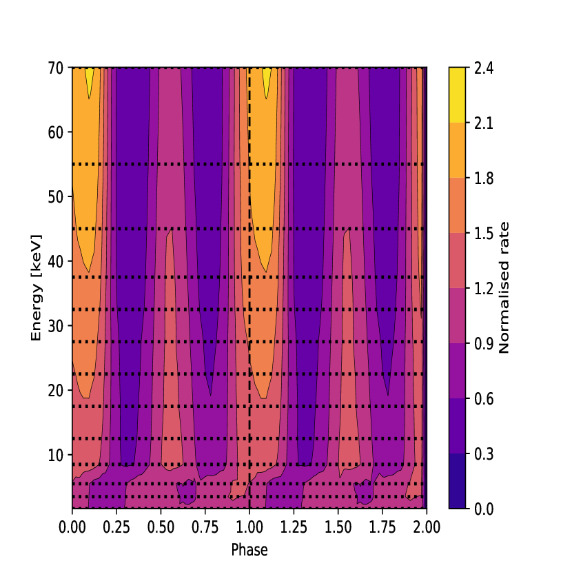
Figure 5: Energy-resolved pulse profiles for J0243 from SXT and LAXPC data of Obs–1 (Left) and Obs–2 (Right). Yellow (Purple) colour correspond to higher (lower) count rates at different phases and energies. Horizontal cuts are pulse profiles for the selected energy range while the vertical cut represent spectra during one complete rotation cycle.

Figure 6: Pulse fraction variation of J0243 as a function of energy for Obs–1 (Left) and Obs–2 (Right). The horizontal bars represent the energy bins used.

4 Spectral Analysis and Results

We have performed spectral fitting using XSPEC v-12.9.0 (Arnaud, 1996). The extracted SXT and LAXPC spectra were grouped using the FTOOLS task ‘grppha’ to have a minimum of 25 counts per bin. We have used the 1-7 keV energy range of SXT and ignored data below 1 keV to avoid systematic uncertainties in the calibration at very low energies. For Obs–1, we found that the LAXPC background dominates at higher energies (see Appendix A) and, in order to avoid an undesirable contribution from instrumental systematics, we considered only the 4-25 keV energy range when performing spectral fitting. For Obs–2 the energy range of 4-70 keV was used. To include the effects of Galactic absorption we used the ‘tbabs’ model component with abundances from Wilms et al. (2000) and cross-sections as given by Verner et al. (1996). A multiplicative term (CONSTANT) was added to the model to account for calibration uncertainties between SXT and LAXPC. This factor was fixed to 1 for the SXT data and was allowed to vary for LAXPC20.

Accretion-powered X-ray pulsars radiate powerfully over a wide energy range, from thermal seed photons at soft X-rays to the reprocessed emission (inverse Comptonization of thermal seed photons) at hard X-rays. Their broadband continuum spectra are typically described with a combination of a black-body (for the low energy excess) and a power law with quasi-exponential high energy cut-offs of various forms. One of the most widely used continuum models has a high energy exponential cut-off (see e.g., White et al., 1983; Mihara et al., 1995; Coburn et al., 2002; Fürst et al., 2014).

The continuum emission of J0243 obtained with NuSTAR and HXMT was studied using an absorbed black-body (bbodyrad) and a cut-off power law (cutoffpl) model (Bahramian et al., 2017; Jaisawal et al., 2018; Zhang et al., 2019). There also exist other phenomenological XSPEC models such as high energy cut-off power law (‘highecut’), a combination of two negative and positive power laws with exponential cutoff (‘NPEX’). Other local models such as power law with Fermi-Dirac cut-off (‘fdcut’; Tanaka, 1986) and a smooth high energy cut-off model (‘newhcut’; Burderi et al., 2000) are also often used to study the spectra of accretion-powered pulsars. We tried to model the continuum emission of J0243 using all of them (see Tables 3,4). The SXT spectra were corrected for gain offset during the observations using the gain fit command with fixed slope of 1.0 and best fit offset of $\sim$ 0.09 eV. An offset correction of 0.03–0.09 keV is needed in quite a few SXT observations.

The following two models provided better fits to the J0243 spectra of Obs–1, in terms of absence of systematic residuals and smaller $\chi^{2}_{\nu}$ values: tbabs*(highecut*powerlaw+bbodyrad), tbabs*(newhcut*powerlaw+bbodyrad), where ‘newhcut’ is the modified version of the high energy cut-off model, smoothed around the cut-off energy. The mathematical form of this model can be found in Burderi et al. (2000). The constants in this model are calculated internally assuming the continuity of the intensity function and its derivative in the range of $E_{C}\pm{\bigtriangleup}E$. We fixed ${\bigtriangleup}E$ to 5.0 keV while performing the spectral fitting. This was done for consistency with the method adopted in the spectral study of accretion powered pulsars using this model (see e.g., Jaisawal & Naik, 2015; Maitra et al., 2017). We added a systematic error of 1% over the entire 1-25.0 keV energy band. In Table 3, we give the best-fit parameters and 90 $\%$ confidence ranges obtained with these models.
The presence of a neutral iron $K_{\alpha}$ line at 6.4 keV was detected in NuSTAR spectra of J0243 (Jaisawal et al., 2018; Tao et al., 2019). Therefore, we tried adding a Gaussian component to the above-mentioned best-fit continuum models, however, we found that a neutral iron $K_{\alpha}$ line is statistically not required.

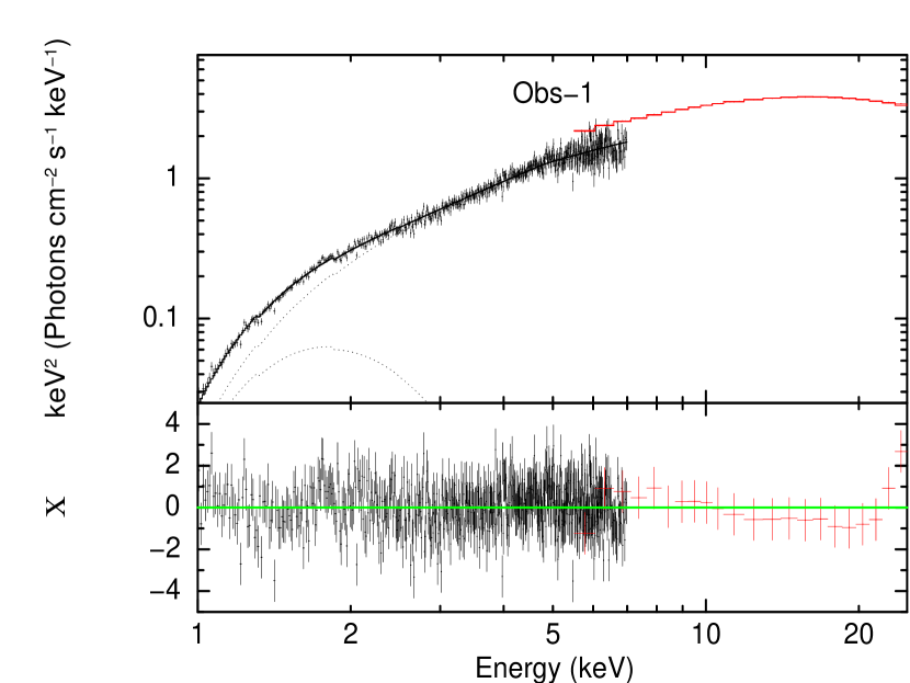
Figure 7: AstroSat spectral data from J0243 and model component fits to detectors SXT, LAXPC for Obs–1 (1–25 keV; Left) and Obs–2 (1–70. keV; Right). The 30 keV Gaussian is due to the calibration Xenon Edge. These unfolded spectra are plotted using eeuf in XSPEC, corresponding to units of ${\nu}f_{\nu}$. The best-fit obtained using Model 1 of Obs–1 and Obs–2 are shown.

The same continuum spectral models as above were first tried to fit the spectral data of Obs–2. However, we found that the four component models used in the first observation were inadequate to give a good (or acceptable) fit to the data. Residuals around 30 keV due to the Xenon calibration edge (Antia et al. 2017) were observed in the LAXPC20 spectra and were modeled using a Gaussian. A similar feature has also been found in the LAXPC spectra of other sources (see e.g., Sharma et al., 2020; Banerjee et al., 2020). We also added a larger systematic ($3{\%}$) value to account for uncertainties in response calibration over such a wide energy band 4-70 keV (see e.g., Mudambi et al., 2020).  Additional systematic residuals at low energies were also observed, therefore, following Tao et al. (2019) we added an additional black-body component (bbodyrad) to the spectra. This black-body component may be associated with the thermal emission from the photosphere of optically-thick outflows or from the extended accretion column as proposed for the case of super-Eddington accretion. We observed that reasonably good fits were obtained by addition of this component to the model (see Figure 7). We also found that spectral fits required an additional Gaussian component to fit the iron emission feature observed at around 6.9 keV. As it was difficult to constrain all the line parameters, therefore, we fixed the line width to 0.5 keV. The best-fit parameters are given in Table 4. From this table, we can see that Model 1 tbabs*(highecut*powerlaw+bbodyrad+bbodyrad
+gaussian) describes the broad-band spectra well and, therefore, to compute the significance of the detected iron emission line, we have used Model 1. We found that on adding this additional Gaussian component at around 6.9 keV, the value of $\chi^{2}$ decreased from 643(628) to 615(626) for 2 degrees of freedom, corresponding to an F value of 13.8, and an F-test false alarm probability of $1.3\times 10^{-6}$. This suggests that the detection of an iron line feature is statistically significant.

To further investigate the significance of this emission feature we simulated 10,000 spectra assuming the tbabs*(highecut*powerlaw+bbodyrad+bbodyrad) model to be true. We searched for the presence of an iron line in each of these data sets by comparing the best fit $\chi^{2}$ values with and without a Gaussian component. We then compared the F statistic of each simulation against that for the observed data. Finally, we infer the probability of a chance improvement of $\chi^{2}$ by counting how many times the simulated values of F were larger than obtained from the real data. In all cases, the estimated chance probability was lower than observed in the real data, implying a significance of $3.9~{}{\sigma}$.

5 Discussion

AstroSat observed J0243 twice during its 2017-18 outburst, and we have analysed data obtained over a broad energy range (0.3-150 keV) with all three of its X-ray instruments. In Section 5.1 we discuss the results of our timing study, while Section 5.2 addresses the spectroscopic results.

5.1 Evolution of the Pulse Profiles

J0243 was accreting at sub-Eddington level during Obs–1, while during Obs–2 the pulsar was super-Eddington. We probed the light curves extracted in narrow energy bands and found that significant pulsations were detected up to 150 keV during Obs–2. However, for the relatively fainter observation (Obs–1), pulsations were detected only up to 80 keV. The average pulse profiles revealed a double-peaked behaviour during both observations, separated by $\sim$ 19 days. The existence of two peaks in the pulse profiles can be due to the contribution from both magnetic poles of the neutron star or two sides of a fan beam from one pole. The pulse profiles created using data from each instrument showed a strong energy dependence. During Obs–1 the soft energy pulse profiles are quite complex compared to higher energies, while for Obs–2, the pulse profiles in all energy bands are relatively simpler, but the modulation is much larger at higher energies. Differences seen in the pulse profiles of these two observations could be due to changes in their accretion levels. WH18 also observed similar dependence of the pulse profiles on the X-ray luminosity using data from NICER and FERMI-GBM, however, the AstroSat data allowed us to probe into these profiles up to 150 keV using narrow energy bands. Luminosity dependence of the pulse profiles has also been observed in several other X-ray pulsars (see e.g., White et al., 1983; Nagase, 1989; Doroshenko et al., 2020, and references therein).

During these observations (Obs–1 & Obs–2), we found that the PF of both peaks in the pulse profiles showed an increase with energy. This indicates that the higher energy photons contribute to the X-ray pulsations. Tao et al. (2019) performed a PF evolution study using the 5 NuSTAR observations, revealing that the PF increased with increasing energy when J0243 was super-Eddington. They suggested that the cut-off power law dominates towards higher energies, and is responsible for the associated increase in PF, as also observed in our pulse profiles of Obs–2. We note that the pulse profiles of NGC 300 ULX1 also showed similar high values of PF (see Carpano et al., 2018). Moreover, during the 2016 super-Eddington outburst of SMC X–3 (Townsend et al., 2017) a smooth increase in the PF with energy was observed (Tsygankov et al., 2017), similar to that observed during Obs–2 when J0243 was accreting at a super-Eddington level. In a few X-ray pulsars it has been found that close to the cyclotron line energies PF shows a non-monotonic dependence on energy (see e.g., Tsygankov et al., 2007). Thus, the smooth behaviour observed is consistent with the fact that we do not observe any strong features (e.g., CRSF) in the source energy spectrum.

5.2 Broadband Spectroscopy

The best fit to the spectra of Obs–1 was obtained using the following model: tbabs*(highecut*powerlaw+bbodyrad) while for Obs–2 we required two additional model components: a hot $\sim$ 1.2 keV black-body and a Gaussian ($\sim$6.9 keV) component to obtain the best fit. Assuming a distance of 7 kpc, the unabsorbed X-ray flux measured during the first and second observations translates to $L_{X}$ of $7.4\times 10^{37}$ and $6.3\times 10^{38}\rm erg~{}s^{-1}$ in the 1-70 keV band, respectively. This indicates that during the first AstroSat observation the source was accreting at sub-Eddington level, increasing to super-Eddington during the second observation. Becker et al. (2012) and Mushtukov et al. (2015) calculated the critical luminosity ($L_{c}$) of a neutron star which marks the transition between the coulomb-dominated and radiation-dominated accretion flow. Assuming canonical neutron star parameters they found that $L_{c}$ is of the order of $10^{37}~{}\rm{erg~{}s^{-1}}$. However, results obtained using NICER and Fermi-GBM suggested that J0243 has a much higher value of $L_{c}$ of the order of $\sim$ $10^{38}\rm{erg~{}s^{-1}}$ (for details see WH18). Thus, it seems that during Obs–1 the source was in its sub-critical accretion regime while during Obs–2 it was super-critical. This is also evident from prominent changes observed in the pulse profiles of J0243 during Obs–1 and 2 (see Section 5.1).

During Obs–1, we observed the black-body temperature to be 0.3-0.4 keV, arising from a radius of about $25-38$ km. For Obs–2 the two values of temperature found are $\sim$ 0.4 keV and 1.2 keV and the estimated values of black-body radius are about $121-142$ km and $18-19$ km, respectively. Tao et al. (2019) studied the spectra of J0243 using NuSTAR and observed a blackbody temperature of about 2–3 keV during the sub-Eddington accretion level. This thermal emission is thought to be arising from the hot spot of a neutron star which gets hotter (4.5 keV) during the super-Eddington phase, with Tao et al. (2019) suggesting that two additional black-body components with temperatures of about 1.5 keV and 0.5 keV are needed during the super-Eddington accretion level. Based on the radius measurements, the origin of these additional black-body components is suggested to be the top of the accretion column and optically thick outflows, respectively. Therefore, it may be possible that the thermal emission observed at a temperature of about 1.2 keV during Obs–2 is due to the emission from the accretion column while the origin of the lower temperature ($0.38$ keV) black-body component is due to the possible presence of optically-thick outflows.
However, we note that a recent study Jaisawal et al. (2019) suggested that, in the ultra-luminous state, the iron line is complex, and if accurately modelled, then the 2 additional black-body components are not required at extreme luminosity.

Mushtukov et al. (2017) proposed that during super-Eddington accretion, the presence of an accretion envelope plays a key role in the accretion process at extreme mass accretion rates. It is expected to significantly modify the timing and spectral properties of ULPs, with smoother more sinusoidal pulse profiles observed and a softer X-ray spectrum due to the reprocessing of the photons emitted from near the neutron star by the optically-thick accretion envelope. J0243 exhibits complex pulse profiles at lower energies, and the pulsed emission is observed up to 150keV. The observed black-body temperature is also much lower than what is expected for the accretion envelopes around ULPS (${\geq}$ 1 keV). The absence of signatures for reprocessing the central emission in J0243 may, however, be attributed to its lower accretion rate than in the classical ULPS ($L_{X}{\sim}10^{40}\rm{erg~{}s^{-1}}$), in which case the opacity of the accretion envelope is not enough to reprocess most of the emission from the central compact object. Interestingly, other X-ray pulsars with very high accretion rates; SMC X–3 (Tsygankov et al., 2017) and NGC 300  ULX1 (Carpano et al., 2018) albeit with lower $L_{X}$ than the classical ULPs, also exhibit complex pulse profiles and high pulsed fractions. These sources might therefore act as an important connecting bridge between the classical X-ray pulsars and ULPs.

Jaisawal et al. (2019) found a narrow 6.42 keV line when the source was in the sub-Eddington regime. The absence of an iron emission feature in the LAXPC spectra (when the source was accreting at a sub-critical level) could be due to the limited energy resolution of the instrument, which is $\sim$$20\%$ at 6.4 keV (see Yadav et al., 2017). As an example, Sharma et al. (2020) did not find any residuals around 6.4 keV in the combined spectra of SXT and LAXPC, while systematic residuals were seen in the simultaneously observed XMM-Newton spectra. As the pulsar luminosity approaches the Eddington limit (${\sim}1.8{\times}10^{38}{\rm{ergs^{-1}}}$ for a $1.4M_{\odot}$ neutron star), the iron line broadens, with significant contributions from 6.67 keV (Fe XXV), and 6.97 keV (Fe XXVI) features (see Jaisawal et al., 2019, for details). Thus, this might be the reason that we observed an emission line feature at around 6.9 keV with LAXPC during Obs–2.

Table 3: Spectral fit parameters of Obs–1 with phenomenological models (1–25 keV).

Parameters	Model 1	Model 2	Model 3	Model 4	Model 5
		Obs–1 (T01_193T01_9000001590)
$N\rm{{}_{H}}$ ($10^{22}\rm{cm^{-2}}$)	$0.93\pm 0.05$	$1.10\pm{-0.07}$	$1.03\pm 0.06$	$0.97\pm 0.06$	$1.21\pm 0.07$
$\Gamma$	$0.58\pm 0.04$	$0.45\pm 0.03$	$0.25\pm 0.03$	$0.63\pm 0.05$	$0.69\pm 0.03$
$E_{cut}$ (keV)	$4.8\pm 0.2$	$10.2\pm{0.3}$	$7.1\pm 0.4$	$5.36_{-0.22}^{+0.21}$	$1~{}(fixed)$
$E_{fold}$ (keV)	$11.3\pm 0.4$	-	-	$11.6_{-0.10}^{+0.05}$	$9.8\pm 0.2$
$kT\rm_{bb}~{}(keV)$	$0.33\pm 0.02$	$0.26\pm 0.01$	$0.28\pm 0.01$	$0.30\pm 0.01$	$0.23\pm 0.01$
$N^{a}$	$0.142\pm 0.007$	$0.178\pm 0.008$	$0.158\pm 0.006$	$0.153\pm 0.01$	$0.39\pm 0.02$
$const_{LAXPC}$	$1.20\pm 0.02$	$1.20\pm 0.02$	$1.20\pm 0.02$	$1.20\pm 0.02$	$1.20\pm 0.02$
${UnabsorbedFlux(1-25keV)}^{b}$	$1.02\pm 0.04$	$1.02\pm 0.04$	$1.02\pm 0.04$	$1.02\pm 0.04$	$1.02\pm 0.04$
${UnabsorbedFlux(1-70keV)}^{b}$	$1.26\pm 0.04$	$1.26\pm 0.04$	$1.26\pm 0.04$	$1.26\pm 0.04$	$1.26\pm 0.04$
Reduced ${\chi}^{2}$ (dof)	1.13 (580)	1.36 (581)	1.26 (580)	1.19 (580)	1.52 (580)

Note: a $\rightarrow$ Normalization ($N$) is in units of $\rm{photons~{}cm}^{-2}~{}\rm{s}^{-1}~{}\rm{keV}^{-1}$ at 1 keV.

b $\rightarrow$ Unabsorbed flux in units $10^{-8}ergs\,cm^{-2}s^{-1}$

c $\rightarrow$ fixed parameters

Model 1: const*tbabs*(powerlaw*highecut+bbodyrad)

Model 2: const*tbabs*(cutoffpl+bbodyrad)

Model 3: const*tbabs*(NPEX+bbodyrad)

Model 4: const*tbabs*(powerlaw*newhcut+bbodyrad)

Model 5: const*tbabs*(powerlaw*fdcut+bbodyrad)

Table 4: Spectral fit parameters of Obs–2 with phenomenological models (1–70 keV).

Parameters	Model 1	Model 2	Model 3	Model 4	Model 5
		Obs–2 (ObsID T01_202T01_9000001640)
$N\rm{{}_{H}}$ ($10^{22}\rm{cm^{-2}}$)	$0.72\pm 0.03$	$0.74\pm{-0.03}$	$0.72\pm 0.03$	$0.72\pm 0.03$	$0.76\pm 0.02$
$\Gamma$	$0.69_{-0.05}^{+0.09}$	$0.67\pm 0.08$	$0.39\pm 0.06$	$0.7\pm 0.1$	$0.95\pm 0.07$
$E_{cut}$ (keV)	$4.2\pm 0.3$	$17.5\pm{0.8}$	$12.4\pm 0.2$	$11.6_{-0.22}^{+0.21}$	$1~{}(fixed)$
$E_{fold}$ (keV)	$18\pm 1$	-	-	$18\pm 1$	$17.9\pm 0.7$
$kT1\rm_{bb}~{}(keV)$	$1.24\pm 0.03$	$1.25\pm 0.02$	$1.24\pm 0.02$	$1.28\pm 0.01$	$1.28\pm 0.01$
$kT2\rm_{bb}~{}(keV)$	$0.38\pm 0.01$	$0.37\pm 0.01$	$0.37\pm 0.01$	$0.38\pm 0.01$	$0.36\pm 0.01$
$E_{Fe}$ (keV)	$6.9\pm 0.3$	$6.9\pm 0.3$	$6.9\pm 0.3$	$6.9\pm{0.3}$	$6.9\pm 0.3$
$EW_{Fe}$ (eV)	$137_{-96}^{+34}$	$40\pm 20$	$159_{-119}^{+6}$	$165_{-115}^{+27}$	$130_{-110}^{+15}$
$N^{a}$	$0.9^{+0.3}_{-0.2}$	$1.1\pm 0.2$	$0.7\pm 0.1$	$0.64\pm 0.01$	$3.4\pm 0.6$
$const_{LAXPC}$	$1.20\pm 0.02$	$1.20\pm 0.02$	$1.20\pm 0.02$	$1.20\pm 0.02$	$1.20\pm 0.02$
${UnabsorbedFlux(1-70keV)}^{b}$	$10.78\pm 0.04$	$10.78\pm 0.04$	$10.78\pm 0.04$	$10.78\pm 0.04$	$10.78\pm 0.04$
Reduced ${\chi}^{2}$ (dof)	0.98 (626)	1.00 (630)	0.99 (630)	0.99 (626)	1.02 (630)

Note: a $\rightarrow$ Normalization ($N$) is in units of $\rm{photons~{}cm}^{-2}~{}\rm{s}^{-1}~{}\rm{keV}^{-1}$ at 1 keV.

b $\rightarrow$ Unabsorbed flux in units $10^{-8}ergs\,cm^{-2}s^{-1}$

c $\rightarrow$ fixed parameters

Model 1: const*tbabs*(powerlaw*highecut+bbodyrad+bbodyrad+gaussian)

Model 2: const*tbabs*(cutoffpl+bbodyrad+bbodyrad+gaussian)

Model 3: const*tbabs*(NPEX+bbodyrad+bbodyrad+gaussian)

Model 4: const*tbabs*(powerlaw*newhcut+bbodyrad+bbodyrad+gaussian)

Model 5: const*tbabs*(powerlaw*fdcut+bbodyrad+bbodyrad+gaussian)

6 Summary

• AstroSat observations of J0243 performed during its 2017-2018 outburst have allowed us to detect pulsations up to 150 keV. These observations were made during two different levels of accretion viz., sub-Eddington ($L_{X}~{}{\sim}~{}7{\times}10^{37}~{}\rm{erg~{}s^{-1}}$) and super-Eddington ($L_{X}~{}{\sim}~{}6{\times}10^{38}~{}\rm{erg~{}s^{-1}}$).

• Pulse profiles show a strong energy and luminosity dependence which is consistent with results from NICER and Fermi–GBM.

• Our study of broad-band X-ray spectra does not show any dip-like feature indicative of a cyclotron line.

• Spectral data from observations made at the sub-Eddington level could be modeled well using an absorbed high energy cut-off power law and a blackbody. Data obtained during the super-Eddington phase of the source, however, requires additional components such as another blackbody and a Gaussian component for the iron emission line.

• The presence of two blackbodies: one with a radius of $18-19~{}\rm{km}$ for the high temperature one, and another with a radius of $121-142~{}\rm{km}$ for the low temperature one, possibly indicates contribution to thermal emission from the accretion column and optically-thick outflows.

DATA AVAILABILITY

The data underlying this article are publicly available in ISSDC, at https://astrobrowse.issdc.gov.in/astroarchive/archive/Home.jsp

Appendix A LAXPC20 source+background and background spectra during Obs–1 and Obs–2

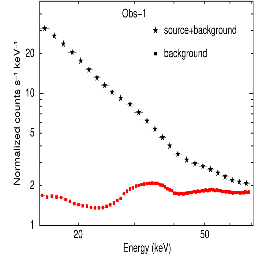
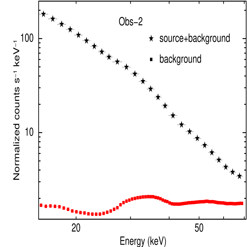
Figure 8: Plot showing LAXPC20 source+background and background spectra simultaneously in the 15–70 keV energy band. An instrumental artifact, a bump at around $\sim$33$\rm{keV}$ (Antia et al., 2017) can be seen in both figures with background dominance at higher energies during Obs–1 in comparison to Obs–2. Although the signal to noise ratio indicates that the energy range can be extended to higher energies, but systematic features dominate the spectrum of Obs–1.

References

- Agrawal (2006) Agrawal P. C., 2006, Advances in Space Research, 38, 2989
- Antia et al. (2017) Antia H. M., et al., 2017, ApJS, 231, 10
- Arnaud (1996) Arnaud K. A., 1996, in Jacoby G. H., Barnes J., eds, Astronomical Society of the Pacific Conference Series Vol. 101, Astronomical Data Analysis Software and Systems V. p. 17
- Bachetti et al. (2014) Bachetti M., et al., 2014, Nature, 514, 202
- Bahramian et al. (2017) Bahramian A., Kennea J. A., Shaw A. W., 2017, The Astronomer’s Telegram, 10866, 1
- Banerjee et al. (2020) Banerjee A., Bhattacharjee A., Chatterjee D., Debnath D., Chakrabarti S. K., Katoch T., Antia H. M., 2020, arXiv e-prints, p. arXiv:2007.05273
- Beardmore et al. (2017) Beardmore A. P., et al., 2017, GRB Coordinates Network, 21971, 1
- Becker et al. (2012) Becker P. A., et al., 2012, A&A, 544, A123
- Bhalerao et al. (2017) Bhalerao V., et al., 2017, Journal of Astrophysics and Astronomy, 38, 31
- Bikmaev et al. (2017) Bikmaev I., et al., 2017, The Astronomer’s Telegram, 10968, 1
- Boldin et al. (2013) Boldin P. A., Tsygankov S. S., Lutovinov A. A., 2013, Astronomy Letters, 39, 375
- Burderi et al. (2000) Burderi L., Di Salvo T., Robba N. R., La Barbera A., Guainazzi M., 2000, ApJ, 530, 429
- Carpano et al. (2018) Carpano S., Haberl F., Maitra C., Vasilopoulos G., 2018, MNRAS, 476, L45
- Cenko et al. (2017) Cenko S. B., et al., 2017, GRB Coordinates Network, 21960, 1
- Coburn et al. (2002) Coburn W., Heindl W. A., Rothschild R. E., Gruber D. E., Kreykenbohm I., Wilms J., Kretschmar P., Staubert R., 2002, ApJ, 580, 394
- Currie et al. (2014) Currie M. J., Berry D. S., Jenness T., Gibb A. G., Bell G. S., Draper P. W., 2014, in Manset N., Forshay P., eds, Astronomical Society of the Pacific Conference Series Vol. 485, Astronomical Data Analysis Software and Systems XXIII. p. 391
- Doroshenko et al. (2018) Doroshenko V., Tsygankov S., Santangelo A., 2018, A&A, 613, A19
- Doroshenko et al. (2020) Doroshenko V., et al., 2020, MNRAS, 491, 1857
- Fürst et al. (2014) Fürst F., et al., 2014, ApJ, 784, L40
- Fürst et al. (2016) Fürst F., et al., 2016, ApJ, 831, L14
- Horne & Baliunas (1986) Horne J. H., Baliunas S. L., 1986, ApJ, 302, 757
- Israel et al. (2017) Israel G. L., et al., 2017, MNRAS, 466, L48
- Jaisawal & Naik (2015) Jaisawal G. K., Naik S., 2015, MNRAS, 448, 620
- Jaisawal et al. (2018) Jaisawal G. K., Naik S., Chenevez J., 2018, MNRAS, 474, 4432
- Jaisawal et al. (2019) Jaisawal G. K., et al., 2019, ApJ, 885, 18
- Jenke & Wilson-Hodge (2017) Jenke P., Wilson-Hodge C. A., 2017, The Astronomer’s Telegram, 10812, 1
- Kaaret et al. (2017) Kaaret P., Feng H., Roberts T. P., 2017, ARA&A, 55, 303
- Kennea et al. (2017) Kennea J. A., Lien A. Y., Krimm H. A., Cenko S. B., Siegel M. H., 2017, The Astronomer’s Telegram, 10809, 1
- Kouroubatzakis et al. (2017) Kouroubatzakis K., Reig P., Andrews J., ) A. Z., 2017, The Astronomer’s Telegram, 10822, 1
- Leahy (1987) Leahy D. A., 1987, A&A, 180, 275
- Lomb (1976) Lomb N. R., 1976, Ap&SS, 39, 447
- Maitra et al. (2017) Maitra C., Raichur H., Pradhan P., Paul B., 2017, MNRAS, 470, 713
- Mihara et al. (1995) Mihara T., Makishima K., Nagase F., 1995, in American Astronomical Society Meeting Abstracts. p. 104.03
- Mudambi et al. (2020) Mudambi S. P., Maqbool B., Misra R., Hebbar S., Yadav J. S., Gudennavar S. B., S. G. B., 2020, ApJ, 889, L17
- Mushtukov et al. (2015) Mushtukov A. A., Suleimanov V. F., Tsygankov S. S., Poutanen J., 2015, MNRAS, 454, 2539
- Mushtukov et al. (2017) Mushtukov A. A., Suleimanov V. F., Tsygankov S. S., Ingram A., 2017, Monthly Notices of the Royal Astronomical Society, 467, 1202
- Nagase (1989) Nagase F., 1989, PASJ, 41, 1
- Roberts et al. (1987) Roberts D. H., Lehar J., Dreher J. W., 1987, AJ, 93, 968
- Rodríguez Castillo et al. (2020) Rodríguez Castillo G. A., et al., 2020, ApJ, 895, 60
- Sathyaprakash et al. (2019) Sathyaprakash R., et al., 2019, MNRAS, 488, L35
- Scargle (1982) Scargle J. D., 1982, ApJ, 263, 835
- Sharma et al. (2020) Sharma R., Beri A., Sanna A., Dutta A., 2020, MNRAS, 492, 4361
- Singh et al. (2014) Singh K. P., et al., 2014, in Space Telescopes and Instrumentation 2014: Ultraviolet to Gamma Ray. p. 91441S, doi:10.1117/12.2062667
- Singh et al. (2016) Singh K. P., et al., 2016, in Space Telescopes and Instrumentation 2016: Ultraviolet to Gamma Ray. p. 99051E, doi:10.1117/12.2235309
- Singh et al. (2017) Singh K. P., et al., 2017, Journal of Astrophysics and Astronomy, 38, 29
- Sreehari et al. (2019) Sreehari H., Ravishankar B. T., Iyer N., Agrawal V. K., Katoch T. B., Mandal S., Nand i A., 2019, MNRAS, 487, 928
- Tanaka (1986) Tanaka Y., 1986, Observations of Compact X-Ray Sources. p. 198, doi:10.1007/3-540-16764-1˙12
- Tao et al. (2019) Tao L., Feng H., Zhang S., Bu Q., Zhang S., Qu J., Zhang Y., 2019, ApJ, 873, 19
- Townsend et al. (2017) Townsend L. J., Kennea J. A., Coe M. J., McBride V. A., Buckley D. A. H., Evans P. A., Udalski A., 2017, MNRAS, 471, 3878
- Tsygankov et al. (2007) Tsygankov S., Lutovinov A., Churazov E., Sunyaev R., 2007, in The Obscured Universe. Proceedings of the VI INTEGRAL Workshop. p. 403 (arXiv:astro-ph/0610476)
- Tsygankov et al. (2017) Tsygankov S. S., Doroshenko V., Lutovinov A. A., Mushtukov A. A., Poutanen J., 2017, A&A, 605, A39
- Tsygankov et al. (2018) Tsygankov S. S., Doroshenko V., Mushtukov A. e. A., Lutovinov A. A., Poutanen J., 2018, MNRAS, 479, L134
- Vadawale et al. (2016) Vadawale S. V., et al., 2016, in Space Telescopes and Instrumentation 2016: Ultraviolet to Gamma Ray. p. 99051G (arXiv:1609.00538), doi:10.1117/12.2235373
- Verner et al. (1996) Verner D. A., Ferland G. J., Korista K. T., Yakovlev D. G., 1996, ApJ, 465, 487
- White et al. (1983) White N. E., Swank J. H., Holt S. S., 1983, ApJ, 270, 711
- Wilms et al. (2000) Wilms J., Allen A., McCray R., 2000, ApJ, 542, 914
- Wilson-Hodge et al. (2018) Wilson-Hodge C. A., et al., 2018, ApJ, 863, 9
- Yadav et al. (2016) Yadav J. S., et al., 2016, Proc. SPIE, 9905, 99051D
- Yadav et al. (2017) Yadav J. S., Agrawal P. C., Antia H. M., Manchand a R. K., Paul B., Misra R., 2017, arXiv e-prints, p. arXiv:1705.06440
- Zhang et al. (2019) Zhang Y., et al., 2019, arXiv e-prints, p. arXiv:1906.01938