Formal Verification of Robustness and Resilience of
Learning-Enabled State Estimation Systems

Abstract

This paper presents a formal verification guided approach for a principled design and implementation of robust and resilient learning-enabled systems. We focus on learning-enabled state estimation systems (LE-SESs), which have been widely used in robotics applications to determine the current state (e.g., location, speed, direction, etc.) of a complex system. The LE-SESs are networked systems composed of a set of connected components including: Bayes filters for localisation, and neural networks for processing sensory input. We study LE-SESs from the perspective of formal verification, which determines the satisfiabilty of a system model against the specified properties. Over LE-SESs, we investigate two key properties – robustness and resilience – and provide their formal definitions. To enable formal verification, we reduce the LE-SESs to a novel class of labelled transition systems, named {PO}²-LTS in the paper, and formally express the properties as constrained optimisation objectives. We prove that the robustness verification is NP-complete. Based on {PO}²-LTS and the optimisation objectives, practical verification algorithms are developed to check the satisfiability of the properties on the LE-SESs. As a major case study, we interrogate a real-world dynamic tracking system which uses a single Kalman Filter (KF) – a special case of Bayes filter – to localise and track a ground vehicle. Its perception system, based on convolutional neural networks, processes a high-resolution Wide Area Motion Imagery (WAMI) data stream. Experimental results show that our algorithms can not only verify the properties of the WAMI tracking system but also provide representative examples, the latter of which inspired us to take an enhanced LE-SESs design where runtime monitors or joint-KFs are required. Experimental results confirm the improvement of the robustness of the enhanced design.

[1]organization=Purple Mountain Laboratories, country=China

[2]organization=University of Liverpool, country=UK

[3]organization=University of Manchester, country=UK

[6]organization=National Digital Switching System Engineering and Technological Research Center, country=China

1 Introduction

An autonomous system is a complex, intelligent system that can make decisions according to its internal state and its understanding about the external environment. To meet their design requirements, autonomous systems can be designed and implemented by connecting a number of heterogeneous components [4] – a form of networked system. In this paper, we consider a typical class of autonomous systems that have been widely used in robotics applications, i.e., state estimation systems (SESs). A SES is used to determine the current state (e.g., location, speed, direction, etc.) of a dynamic system such as a spacecraft or a ground vehicle. Typical applications of SESs in a robotics context include localisation [5], tracking [6], and control [7]. Moreover, with more and more robotics applications adopting deep neural network components to take advantage of their high prediction precision [8], we focus on those SESs with Deep Neural Network (DNN) components, and call them learning-enabled SESs, or LE-SESs.

Typically, in LE-SESs, neural networks are employed to process perceptional input received via sensors. For example, Convolutional Neural Networks (CNNs) are usually taken to process imagery inputs. For a real-world system – such as the Wide Area Motion Imagery (WAMI) tracking system which we will study in this paper – the perceptional unit may include multiple neural networks, which interact to implement a complex perceptional function. In addition to the perception unit, LE-SESs use other components – such as Bayes filters – to estimate, update, and predict the state.

However, neural networks have been found to be fragile, for example they are vulnerable to adversarial attacks [9], i.e., an imperceptibly small but valid perturbation on the input may incorrectly alter the classification output. Several approaches have been developed to study the robustness of neural networks, including adversarial attacks [9, 10, 11], formal verification [12, 13, 14, 15, 16, 17, 18, 19, 20, 21], and coverage-guided testing [22, 23, 24, 25, 26, 27, 28, 29]. All of these contribute to understanding the trustworthiness (i.e. the confidence that a system will provide an appropriate output for a given input) of systems containing deep neural networks; a recent survey can be found at [30]. As will be explained in the paper, for neural networks, robustness is a close concept to resilience. However, it is unclear whether this is the case for the LE-SESs, or more broadly, networked systems with learning components. We will show that, for LE-SESs, there are subtle, yet important, differences between robustness and resilience. Generally, robustness is the ability to consistently deliver its expected functionality by accommodating disturbances to the input, while resilience is the ability to handle and recover from challenging conditions including internal failures and external ‘shocks’, maintaining and/or resuming part (if not all) of its designated functionality. Based on this general view, formal definitions of robustness and resilience on the WAMI tracking system are suggested. In our opinion: robustness quantifies the minimum external effort (of e.g., an attacker) to make a significant change to the system’s functionality–dynamic tracking; and resilience quantifies the supremum (i.e., least upper bound) of the deviation from its normal behaviour from which the system cannot recover. While these two properties are related, we show that they have subtle, yet important, difference from both their formal definitions and the experiments. From the outset, we note that the use of the term robustness in this sense differs from that used in traditional safety engineering. Whilst we continue to apply the prevailing use of term in this paper, we will later urge for alignment with safety engineering to foster the use of Machine Learning (ML) in those applications.

To study the properties of real-world LE-SESs in a principled way, we apply formal verification techniques, which demonstrate that a system is correct against all possible risks over a given specification – a formal representation of property – and the formal model of the system, and which returns counter-examples when it cannot. We adopt this approach to support the necessary identification of risks prior to deployment of safety critical applications. This paper reports the first time a formal verification approach has been developed for state estimation systems.

Technically, we first formalise an LE-SES as a novel labelled transition system which has components for payoffs and partial order relations (i.e. relations that are reflexive, asymmetric and transitive). The labelled transition system is named {PO}²-LTS in the paper. Specifically, every transition is attached with a payoff, and for every state there is a partial order relation between its out-going transitions from the same state. Second, we show that the verification of the properties – both robustness and resilience – on such a system can be reduced into a constrained optimisation problem. Third, we prove that the verification problem is NP-complete for the robustness property on {PO}²-LTS. Fourth, to enable practical verification, we develop an automated verification algorithm.

As a major case study, we work with a real-world dynamic tracking system [7], which detects and tracks ground vehicles over the high-resolution Wide Area Motion Imagery (WAMI) data stream, named WAMI tracking system in this paper. The system is composed of two major components: a state estimation unit and a perceptional unit. The perceptional unit includes multiple, networked CNNs, and the state estimation unit includes one or multiple Kalman filters, which are a special case of Bayes filter. We apply the developed algorithm to the WAMI tracking system to analyse both robustness and resilience, in order to understand whether the system can function well when subject to adversarial attacks on the perceptional neural network components.

The formal verification approach leads to a guided design of the LE-SESs. As the first design, we use a single Kalman filter to interact with the perceptional unit, and our experimental results show that the LE-SES performs very well in a tracking task, when there is no attack on the perceptional unit. However, it may perform less well in some cases when the perceptional unit is under adversarial attack. The returned counterexamples from our verification algorithms indicate that we may improve the safety performance of the system by adopting a better design. Therefore, a second, improved design – with joint-KFs to associate observations and/or a runtime monitor – is taken. Joint-KFs increase the capability of the system in dealing with internal and external uncertainties, and a runtime monitor can reduce some potential risks. We show that in the resulting LE-SES, the robustness is improved, without compromising the precision of the tracking.

The main contributions of this paper are as follows.

1. Robust and resilient LE-SES design: This paper proposes a principled and detailed design of robust and resilient learning-enabled state estimation systems (Section 4).

2. Formal guarantee: The robustness and resilience of the LE-SES is guaranteed by a novel formal verification technique (Sections 5,6,7).

3. Robustness vs resilience: This paper pioneers in aligning the definitions of robustness and resilience in LE-SESs with those applied in traditional high-integrity computing. Their similarity and difference are examined both in theory (Section 6) and in experimental evaluation (Section 8).

In summary, the organisation of the paper is as follows. In the next section, we present preliminaries about neural networks and the Bayes (and Kalman) filters. In Section 3, we introduce our first design of the WAMI-tracking system where a single Kalman filter is used. In Section 4, we present our enhanced design with a runtime monitor and/or joint-KFs. The reduction of LE-SES system to {PO}²-LTS is presented in Section 5. In Section 6, we present a methodological discussion on the difference between robustness and resilience, together with the formalisation of them as optimisation objectives. The automated verification algorithm is presented in Section 7, with the experimental results presented in Section 8. We discuss some aspects on the definitions of robustness and resilience that are not covered in LE-SESs in Section 9. Finally, we discuss related work in Section 10 and conclude the paper in Section 11.

2 Preliminaries

2.1 Convolutional Neural Networks

Let ${\tt X}$ be the input domain and ${\tt Y}$ be the set of labels. A neural network ${N}:{\tt X}\rightarrow{\cal D}({\tt Y})$ can be seen as a function mapping from ${\tt X}$ to probabilistic distributions over ${\tt Y}$. That is, ${N}(x)$ is a probabilistic distribution, which assigns for each label $y\in{\tt Y}$ a probability value $({N}(x))_{y}$. We let $f_{N}:{\tt X}\rightarrow{\tt Y}$ be a function such that for any $x\in{\tt X}$, $f_{N}(x)=\arg\max_{y\in{\tt Y}}\{({N}(x))_{y}\}$, i.e., $f_{N}(x)$ returns the classification.

2.2 Neural Network Enabled State Estimation

We consider a time-series linear state estimation problem that is widely assumed in the context of object tracking. The process model is defined as follows.

$$\mathbf{s}_{k}=\mathbf{F}\cdot\mathbf{s}_{k-1}+\mathbf{\omega}_{k}$$ (1)

where $\mathbf{s}_{k}$ is the state at time $k$, $\mathbf{F}$ is the transition matrix, $\mathbf{\omega}_{k}$ is a zero-mean Gaussian noise such that $\mathbf{\omega}_{k}\sim\mathcal{N}(0,\mathbf{Q})$, with $\mathbf{Q}$ being the covariance of the process noise. Usually, the states are not observable and need to be determined indirectly by measurement and reasoning. The measurement model is defined as:

$$\mathbf{z}_{k}=\mathbf{H}\cdot\mathbf{s}_{k}+\mathbf{v}_{k}$$ (2)

where $\mathbf{z}_{k}$ is the observation, $\mathbf{H}$ is the measurement matrix, $\mathbf{v}_{k}$ is a zero-mean Gaussian noise such that $\mathbf{v}_{k}\sim\mathcal{N}(0,\mathbf{R})$, and $\mathbf{R}$ is the covariance of the measurement noise.

Bayes filters have been used for reasoning about the observations, $\{\mathbf{z}_{k}\}$, with the goal of learning the underlying states $\{\mathbf{s}_{k}\}$. A Bayes filter maintains a pair of variables, $(\mathbf{s}_{k},\mathbf{P}_{k})$, over the time, denoting Gaussian estimate and Bayesian uncertainty, respectively. The basic procedure of a Bayes filter is to use a transition matrix, $\mathbf{F}_{k}$, to predict the current state, $(\hat{\mathbf{s}}_{k},\hat{\mathbf{P}}_{k})$, given the previous state, $(\mathbf{s}_{k-1},\mathbf{P}_{k-1})$. The prediction state can be updated into $(\mathbf{s}_{k},\mathbf{P}_{k})$ if a new observation, $\mathbf{z}_{k}$, is obtained. In the context of the aforementioned problem, this procedure is iterated for a number of time steps, and is always discrete-time, linear, but subject to noises.

We take the Kalman Filter (KF), one of the most widely used variants of Bayes filter, as an example to demonstrate the above procedure. Let $\mathbf{s}_{0}\in{}^{n}\sim{\cal N}(\hat{\mathbf{s}}_{0},\hat{\mathbf{P}}_{0})$ be the initial state, such that $\hat{\mathbf{s}}_{0}\in{}^{n}$ and $\hat{\mathbf{P}}_{0}\in{}^{n\times n}$ represent our knowledge about the initial estimate and the corresponding covariance matrix, respectively.

First, we perform the state prediction for $k\geq 1$:

$$\begin{array}[]{lcl}\hat{\mathbf{s}}_{k}&=&\mathbf{F}_{k}\mathbf{s}_{k-1}\\ \hat{\mathbf{P}}_{k}&=&\mathbf{F}_{k}\mathbf{P}_{k-1}\mathbf{F}_{k}^{T}+\mathbf{Q}_{k}\end{array}$$ (3)

Then, we can update the filter:

$$\begin{array}[]{lcl}\mathbf{s}_{k}&=&\hat{\mathbf{s}}_{k}+\mathbf{K}_{k}\mathbf{y}_{k}\\ \mathbf{P}_{k}&=&(\mathbf{I}-\mathbf{K}_{k}\mathbf{H}_{k})\hat{\mathbf{P}}_{k}\end{array}$$ (4)

where

$$\begin{array}[]{lcl}\mathbf{y}_{k}&=&\mathbf{z}_{k}-\mathbf{H}_{k}\hat{\mathbf{s}}_{k}\\ \mathbf{S}_{k}&=&\mathbf{H}_{k}\hat{\mathbf{P}}_{k}\mathbf{H}_{k}^{T}+\mathbf{R}_{k}\\ \mathbf{K}_{k}&=&\hat{\mathbf{P}}_{k}\mathbf{H}_{k}^{T}\mathbf{S}_{k}^{-1}\end{array}$$ (5)

Intuitively, $\mathbf{y}_{k}$ is usually called “innovation” in signal processing and represents the difference between the real observation and the predicted observation, $\mathbf{S}_{k}$ is the covariance matrix of this innovation, and $\mathbf{K}_{k}$ is the Kalman gain, representing the relative importance of innovation $\mathbf{y}_{k}$ with respect to the predicted estimate $\hat{\mathbf{s}}_{k}$.

In a neural network enabled state estimation, a perception system – which may include multiple CNNs – will provide a set of candidate observations $Z_{k}$, any of which can be chosen as the new observation $\mathbf{z}_{k}$. From the perspective of robotics, $Z_{k}$ includes a set of possible states of the robot, measured by (possibly several different) sensors at time $k$. These measurements are imprecise, and are subject to noise from both the environment (epistemic uncertainty) and the imprecision of sensors (aleatory uncertainty).

3 A Real-World WAMI Dynamic Tracking System

In this part, we present a brief introduction, followed by the technical details, to the real-world WAMI dynamic tracking system that will be used as our major case study. The tracking system requires continuous imagery input from e.g., airborne high-resolution cameras. In the case study, the input is a video, which consists of a finite sequence of WAMI images. Each image contains a number of vehicles. The essential processing chain of the WAMI tracking system is as follows.

1. Align a set of previous frames with the incoming frame.

2. Construct the background model of incoming frames using the median frame.

3. Extract moving objects using background subtraction.

4. Determine if the moving objects are vehicles by using a Binary CNN.

5. For complex cases, predict the locations of moving objects/vehicles using a regression CNN.

6. Track one of the vehicles using a Kalman filter.

WAMI tracking uses Gated nearest neighbour (Gnn) to choose the new observation $\mathbf{z}_{k}$: from the set $Z_{k}$, the one closest to the predicted measurement $\mathbf{H}_{k}\cdot\hat{\mathbf{s}}_{k}$ is chosen, i.e.,

$$\mathbf{z}_{k}=\arg\min_{\mathbf{z}\in Z_{k}}||\mathbf{z}-\mathbf{H}_{k}\cdot\hat{\mathbf{s}}_{k}||_{p}$$ (6)

$$s.t.\quad||\mathbf{z}-\mathbf{H}_{k}\cdot\hat{\mathbf{s}}_{k}||_{p}\leq\tau_{k}$$ (7)

where $||\cdot||_{p}$ is $L^{p}$-norm distance ($p=2$, i.e., Euclidean distance is used in this paper), and $\tau_{k}$ is the gate value, representing the maximum uncertainty in which the system is able to work.

Specifically, the WAMI system has the following definitions of $\mathbf{s}$ and $\mathbf{P}$:

$$\begin{array}[]{lcl}\mathbf{s}&=\begin{bmatrix}\mathbf{l}\\ \mathbf{v}\end{bmatrix}~{}~{}~{}~{}~{}~{}\mathbf{P}&=\begin{bmatrix}\Sigma_{\mathbf{l}\mathbf{l}}&\Sigma_{\mathbf{l}\mathbf{v}}\\ \Sigma_{\mathbf{v}\mathbf{l}}&\Sigma_{\mathbf{v}\mathbf{v}}\end{bmatrix}\end{array}$$ (8)

where $\mathbf{s}$ denotes the mean values of two Gaussian stochastic variables, $\mathbf{l}$ representing the location which is measurable from the input videos, and $\mathbf{v}$, representing the velocity which cannot be measured directly, respectively.

In the measurement space, the elements in $\mathbf{l}$ are not correlated, which makes it possible to simplify the Bayesian uncertainty metric, $\tau$, that is the trace of the covariance matrix:

$$\tau=tr(\Sigma_{\mathbf{l}\mathbf{l}})$$ (9)

Therefore, $\tau$ is partially related to the search range in which observations can be accepted. Normally, $\tau$ will gradually shrink before being bounded – the convergence property of KF as explained below.

3.1 Wide-Area Motion Imagery Input

The input to the tracking system is a video, which consists of a finite sequence of images. Each image contains a number of vehicles. Similar to [31], we use the WPAFB 2009 [32] dataset. The images were taken by a camera system with six optical sensors that had already been stitched to cover a wide area of around $35\,km^{2}$. The frame rate is 1.25Hz. This dataset includes 1025 frames, which is around 13 minutes of video and is divided into training video ($512$ frames) and testing video ($513$ frames), and where all the vehicles and their trajectories are manually annotated. There are multiple resolutions of videos in the dataset. For the experiment, we chose to use the $12$,$000$$\times$$10$,$000$ images, in which the size of vehicles is smaller than $10$$\times$$10$ pixels. We use $\alpha_{i}$ to denote the $i$-th frame and $\alpha_{i}(x,y)$ the pixel on the intersection of $x$-th column and $y$-th row of $\alpha_{i}$.

In the following, we explain how the tracking system works, where video is used as input. In general this is undertaken in two stages: detection and tracking. In Section 3.2 through to Section 3.5, we explain the detection steps, i.e., how to detect a vehicle with CNN-based perception units; this is followed by the tracking step in Section 3.6.

3.2 Background Construction

Vehicle detection in WAMI video is a challenging task due to the lack of vehicle appearances and the existence of frequent pixel noises. It has been discussed in [33, 34], that an appearance-based object detector may cause a large number of false alarms. For this reason, in this paper, we only consider detecting moving objects for tracking.

Background construction is a fundamental step in extracting pixel changes from the input image. The background is built for the current environment from a number of previous frames captured by the moving camera system, through the following steps:

Image registration

Is used to compensate for the camera motion by aligning all the previous frames to the current frame. The key is to estimate a transformation matrix, $h_{k}^{k-t}$, which transforms frame $\alpha_{k-t}$ to frame $\alpha_{k}$ using a given transformation function. For the transformation function, we consider projective transformation (or homography), which has been widely applied in multi-perspective geometry; an area where WAMI camera systems are already utilised.

The estimation of $h_{k}^{k-t}$ is generated by applying feature-based approaches. First of all, feature points from images at frame $\alpha_{k-t}$ and $\alpha_{k}$, respectively, are extracted by feature detectors (e.g., Harris corner or SIFT-like [35] approaches). Second, feature descriptors, such as SURF [36] and ORB [37], are computed for all detected feature points. Finally, pairs of corresponding feature points between two images can be identified and the matrix $h_{k}^{k-t}$ can be estimated by using RANSAC [38], which is robust against outliers.

Background Modeling

We generate the background, $\mathbf{I}_{k}^{bg}$, for each time $k$, by computing the median image of the $L$ previously-aligned frames, i.e.,

$$\mathbf{I}_{k}^{bg}(x,y)=\frac{1}{L}\sum_{i=1}^{L}\alpha_{k-i}(x,y)$$ (10)

In our experiments, we take either $L=4$ or $L=5$.

Note that, to align the $L$ previous frames to the newly received frame, only one image registration process is performed. After obtaining the matrices $h_{k-1}^{k-2},h_{k-1}^{k-3},...$ by processing previous frames, we perform image registration once to get $h_{k}^{k-1}$, and then let

$$h_{k}^{k-2}=h_{k}^{k-1}\times h_{k-1}^{k-2},~{}h_{k}^{k-3}=h_{k}^{k-1}\times h_{k-1}^{k-3}.$$ (11)

Extraction of Potential Moving Objects

By comparing the difference between $\mathbf{I}_{k}^{bg}$ and the current frame $\alpha_{k}$, we can extract a set $Q_{bc}$ of potential moving objects by first computing the following set of pixels

$$P_{bc}=\{(x,y)~{}|~{}|\mathbf{I}_{k}^{bg}(x,y)-\alpha_{k}(x,y)|>\delta_{bc},(x,y)\in\Gamma\}$$ (12)

and then applying image morphology operation on $P_{bc}$, where $\Gamma$ is the set of pixels and $\delta_{bc}$ is a threshold value to determine which pixels should be considered.

3.3 CNN for Detection Refinement

After obtaining $P_{bc}$, we develop a CNN, ${N}_{dr}$, to detect vehicles. We highlight a few design decisions. The major causes of false alarms generated by the background subtraction are: poor image registration, light changes and the parallax effect in high objects (e.g., buildings and trees). We emphasise that the objects of interest (e.g., vehicles) mostly, but not exclusively, appear on roads. Moreover, we perceive that a moving object generates a temporal pattern (e.g., a track) that can be exploited to discern whether or not a detection is an object of interest. Thus, in addition to the shape of the vehicle in the current frame, we assert that the historical context of the same place can help to distinguish the objects of interest and false alarms.

By the above observations, we create a binary classification CNN ${N}_{dr}:{}^{21\times 21\times(m+1)}\xrightarrow{}\{0,1\}$ to predict whether a $21\times 21$ pixels window contains a moving object given aligned image patches generated from the previous $m$ frames. The $21\times 21$ pixels window is identified by considering the image patches from the set $Q_{bc}$. We suggest $m=3$ in this paper, as it is the maximum time for a vehicle to cross the window. The input to the CNN is a $21\times 21\times(m+1)$ matrix and the convolutional layers are identical to traditional 2D CNNs, except that the three colour channels are substituted with $m+1$ grey-level frames.

Essentially, ${N}_{dr}$ acts as a filter to remove, from $Q_{bc}$, objects that are unlikely to be vehicles. Let $Q_{dr}$ be the obtained set of moving objects. If the size of an image patch in $Q_{dr}$ is similar to a vehicle, we directly label it as a vehicle. On the other hand, if the size of the image patch in $Q_{dr}$ is larger than a vehicle, i.e., there may be multiple vehicles, we pass this image patch to the location prediction for further processing.

3.4 CNN for Location Prediction

We use a regression CNN ${N}_{lp}:{}^{45\times 45\times(m+1)}\xrightarrow{}{}^{15\times 15}$ to process image patches passed over from the detection refinement phase. As in [34], a regression CNN can predict the locations of objects given spatial and temporal information. The input to ${N}_{lp}$ is similar to the classification CNN ${N}_{dr}$ described in Section 3.3, except that the size of the window is enlarged to $45\times 45$. The output of ${N}_{lp}$ is a $225$-dimensional vector, equivalent to a down-sampled image ($15\times 15$) for reducing computational cost.

For each $15\times 15$ image, we apply a filter to obtain those pixels whose values are greater than not only a threshold value $\delta_{lp}$ but also the values of its adjacent pixels. We then obtain another $15\times 15$ image with a few bright pixels, each of which is labelled as a vehicle. Let $O$ be the set of moving objects updated from $Q_{dr}$ after applying location prediction.

3.5 Detection Framework

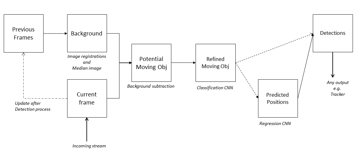
Figure 1: The architecture of the vehicle detector.

The processing chain of the detector is shown in Figure 1. At the beginning of the video, the detector takes the first $L$ frames to construct the background, thus the detections from frame $L+1$ can be generated. After the detection process finishes in each iteration, it is added to the template of previous frames. The updating process substitutes the oldest frame with the input frame. This is to ensure that the background always considers the latest scene, since the frame rate is usually low in WAMI videos such that parallax effects and light changes can be pronounced. As we wish to detect very small and unclear vehicles, we apply a small background subtraction threshold and a minimum blob size. This, therefore, leads to a huge number of potential blobs. The classification CNN is used to accept a number of blobs. As mentioned in Section 3.3, the CNN only predicts if the window contains a moving object or not. According to our experiments, the cases where multiple blobs belong to one vehicle and one blob includes multiple vehicles, occur frequently. Thus, we design two corresponding scenarios: the blob is very close to another blob(s); the size of the blob is larger than $20\times 20$. If any blob follows either of the two scenarios, we do not consider the blob for output. The regression CNN (Section 3.4) is performed on these scenarios to predict the locations of the vehicles in the corresponding region, and a default blob will be given. If the blob does not follow any of the scenarios, this blob will be outputted directly as a detection. Finally, the detected vehicles include the output of both sets.

3.6 Object Tracking

3.6.1 Problem Statement

We consider a single target tracker (i.e. Kalman filter) to track a vehicle given all the detection points over time in the field of view. The track is initialised by manually giving a starting point and a zero initial velocity, such that the state vector is defined as $s_{t}=[x_{t},y_{t},0,0]^{T}$ where $[x_{t},y_{t}]$ is the coordinate of the starting point. We define the initial covariance of the target, $P=diag\left[30,30,20,20\right]^{2}$, which is the initial uncertainty of the target’s state.

A near-constant velocity model is applied as the dynamic model in the Kalman filter, which is defined as follows, by concretising Equation (1).

$$\hat{\mathbf{s}}_{k}=\mathbf{F}\cdot\mathbf{s}_{k-1}+\omega_{k}~{}~{}~{}\text{ s.t. }\mathbf{F}=\left[\begin{array}[]{cccc}\mathbb{I}_{2\times 2}&\mathbb{I}_{2\times 2}\\ \mathbb{O}_{2\times 2}&\mathbb{I}_{2\times 2}\\ \end{array}\right]$$ (13)

where $\mathbb{I}$ is a identity matrix, $\mathbb{O}$ is a zero matrix, and $\mathbf{s}_{k-1},\hat{\mathbf{s}}_{k-1}$ and $\omega_{k}$ are as defined in Section 2, such that the covariance matrix $\mathbf{Q}$ of the process noise is defined as follows:

$$\mathbf{Q}=\sigma_{q}^{2}\cdot\begin{bmatrix}\frac{1}{3}dt^{3}\cdot\mathbb{I}_{2\times 2}&\frac{1}{2}dt^{2}\cdot\mathbb{I}_{2\times 2}\\ \\ \frac{1}{2}dt^{2}\cdot\mathbb{I}_{2\times 2}&\mathbb{I}_{2\times 2}\end{bmatrix}$$ (14)

where $dt$ is the time interval between two frames and $\sigma_{q}$ is a configurable constant. $\sigma_{q}=3$ is suggested for the aforementioned WAMI video.

Next, we define the measurement model by concretising Equation (2):

$$\mathbf{z}_{k}=\mathbf{H}\cdot\mathbf{s}_{k}+\mathbf{v}_{k}\text{\quad s.t. \quad}\mathbf{H}=\left[\begin{array}[]{cccc}1&0&0&0\\ 0&1&0&0\\ \end{array}\right]$$ (15)

where $\mathbf{z}_{k}$ is the measurement representing the position of the tracked vehicle, and $\mathbf{s}_{k}$ and $\mathbf{v}_{k}$ are as defined in Section 2. The covariance matrix, $\mathbf{R}$, is defined as $\mathbf{R}=\sigma_{r}^{2}\cdot\mathbb{I}_{2\times 2}$, where we suggest $\sigma_{r}=5$ for the WAMI video.

Since the camera system is moving, the position should be compensated for such motion using the identical transformation function for image registration. However, we ignore the influence to the velocity as it is relatively small, but consider integrating this into the process noise.

3.6.2 Measurement Association

During the update step of the Kalman filter, the residual measurement should be calculated by subtracting the measurement ($\mathbf{z}_{k}$) from the predicted state ($\hat{\mathbf{s}}_{k}$). In the tracking system, a Gnn is used to obtain the measurement from a set of detections. K-nearest neighbour is first applied to find the nearest detection, $\hat{\mathbf{z}}_{k}$, of the predicted measurement, $\mathbf{H}\cdot\hat{\mathbf{s}}_{k}$. Then the Mahalanobis distance between $\hat{\mathbf{z}_{k}}$ and $\mathbf{H}\cdot\hat{\mathbf{s}}_{k}$ is calculated as follows:

$$D_{k}=\sqrt{(\hat{\mathbf{z}}_{k}-\mathbf{H}\cdot\hat{\mathbf{s}}_{k})^{T}\cdot\hat{\mathbf{S}_{k}}^{-1}\cdot(\hat{\mathbf{z}}_{k}-\mathbf{H}\cdot\hat{\mathbf{s}}_{k})}$$ (16)

where $\hat{\mathbf{P}_{k}}$ is the innovation covariance, which is defined within the Kalman filter.

A potential measurement is adopted if $D_{k}\leq g$ with $g=2$ in our experiment. If there is no available measurement, the update step will not be performed and the state uncertainty accumulates. It can be noticed that a large covariance leads to a large search window. Because the search window can be unreasonably large, we halt the tracking process when the trace of the covariance matrix exceeds a pre-determined value.

4 Improvements to WAMI Tracking System

In this section, we introduce two techniques to improve the robustness and resilience of the LE-SESs. One of the techniques uses a runtime monitor to track a convergence property, expressed with the covariance matrix $\mathbf{P}_{k}$; and the other considers components to track multiple objects around the primary target to enhance fault tolerance in the state estimation.

4.1 Runtime Monitor for Bayesian Uncertainty

Generally speaking, a KF system includes two phases: prediction (Equation (3)) and update (Equation (4)). Theoretically, a KF system can converge [39] with optimal parameters: $\mathbf{F}$, $\mathbf{H}$, $\mathbf{Q}$, and $\mathbf{R}$, that well describe the problem. In this paper, we assume that the KF system has been well designed to ensure the convergence. Empirically, this has been proven possible in many practical systems. We are interested in another characteristic of KF: where the uncertainty, $\hat{\mathbf{P}}_{k}$, increases relative to $\mathbf{P}_{k-1}$, if no observation is available and thus the update phase will not be performed. In such a case, the predicted covariance $\hat{\mathbf{P}}_{k}$ will be treated as the updated covariance $\mathbf{P}_{k}$ in this time-step.

In the WAMI tracking system, when the track does not have associated available observations (e.g., mis-detections) for a certain period of time, the magnitude of the uncertainty metric $\tau$ will be aggregated and finally ‘explode’, and thus the search range of observations is dramatically expanded. This case can be utilised to design a monitor to measure the attack, and therefore should be considered when analysing the robustness and resilience.

The monitor for the Bayesian uncertainty can be designed as follows: when $\tau$ increases, an alarm is set to alert the potential attack. From the perspective of an attacker, to avoid this alert, a successful attack should try to hide the increment of $\tau$. To understand when the increment may appear for the WAMI tracking system, we recall the discussion in Section 3, where a track associates the nearest observation $\mathbf{z}$ within a pre-defined threshold, in Mahalanobis distance, in each time-step. By attacking all the observations in $Z_{k}$, we can create the scenario where no observations are within the search range, which mimics the aforementioned case: the Bayesian uncertainty metric increases due to the skipped update phase.

Formally, we define a parameter $\Gamma$, defined in (17), which monitors the changes of the Kalman filter’s covariance over time and considers the convergence process.

$$\Gamma(\widetilde{\rho}_{k-1},\widetilde{\rho}_{k})=\left\{\begin{array}[]{ll}1&\quad\tau(\widetilde{\rho}_{k})\leq\tau(\widetilde{\rho}_{k-1})\\ 0&\quad\tau(\widetilde{\rho}_{k})>\tau(\widetilde{\rho}_{k-1})\end{array}\right.$$ (17)

4.2 Joining Collaborative Components for Tracking

Reasons for the previous WAMI tracking system malfunctions are two-fold: false alarms and mis-detections. Note that, in this paper, we only track a single target. Using Gnn and a Kalman filter is sufficient to deal with false alarms in most cases. Nevertheless, mis-detection still brings significant issues. As mentioned in Section 4.1, mis-detections may cause the Bayesian uncertainty range to expand. This, compounded with the fact that there are usually many detections encountered in the WAMI videos, leads to the possibility that the tracking is switched to another target. In order to cope with this problem, we consider taking the approach of utilising joining collaborative components and we call it joint Kalman filters (joint-KFs). More specifically, we track multiple targets near the primary target simultaneously with multiple Kalman filters; the detailed process is as follows:

• Two kinds of Kalman filter tracks are maintained: one track for the primary target, $T^{p}$, and multiple tracks for the refining association, $T^{r}$.

• At each time-step other than the initialisation step, we have predicted tracks $\{\hat{T_{k}}^{p},\hat{T_{k}}^{r}\}$, a set $Z_{k}$ of detections from current time-step, and a set $\tilde{Z}_{k-1}$ of unassociated detections from the previous time-step.

  1. Calculate the likelihoods of all the pairs of detections $Z_{k}$ and tracks $\{\hat{T_{k}}^{p},\hat{T_{k}}^{r}\}$ using $\mathcal{N}\left(\hat{\mathbf{s}}_{k},\mathbf{z}_{k},\mathbf{S}_{k}\right)$ where the parameters can be found in Kalman filter.

  2. Sort the likelihoods from the largest to the smallest, and do a gated one-to-one data association in this order.

  3. Perform standard Kalman filter updates for all the tracks.

  4. For each detection in $Z_{k}$ that is not associated and is located close to the primary target, calculate the distance to each element in $Z_{k-1}$.

     • If the distance is smaller than a predefined value, initialize a track and treat the distance as velocity then add this track into $T_{k}^{r}$.

     • Otherwise, store this detection in $\tilde{Z}_{k}$

  5. Maintain all the tracks for refining association, $T_{k}^{r}$: if a track is now far away from the primary target, remove it from the set.

By applying this data association approach, if the primary target is mis-detected, the track will not be associated to a false detection, and even when this occurs for a few time-steps and the search range becomes reasonably large, this system can still remain resilient (i.e. can still function and recover quickly).

5 Reduction of LE-SESs to Labelled Transition Systems

Formal verification requires a formal model of the system, so that all possible behaviour of the system model can be exploited to understand the existence of incorrect behaviour. In this section, we will reduce the LE-SESs to a novel class of labelled transition systems – a formal model – such that all safety-related behaviour is preserved. In the next few sections, we will discuss the formalisation of the properties, the automated verification algorithms, and the experimental results, respectively.

5.1 Threat Model of Adversarial Attack on Perception System

In Section 3, a neural network based perception system determines whether or not there is a vehicle at a location $\mathbf{z}$. Let $x(\mathbf{z})\in{}^{d_{1}\times d_{2}}$ be an image covering the location $\mathbf{z}$, a neural network function $f_{N}:{}^{d_{1}\times d_{2}}\rightarrow\{0,1\}$ maps $x(\mathbf{z})$ into a Boolean value, $f_{N}(x(\mathbf{z}))$, representing whether or not a vehicle is present at location $\mathbf{z}$. There are two types of erroneous detection: (1) a wrong classification prediction of the image $x(\mathbf{z})$, and (2) a wrong positioning of a moving object within $x(\mathbf{z})$. We focus on the former since the WAMI tracking system has a comprehensive mechanism to prevent the occurrence of the latter.

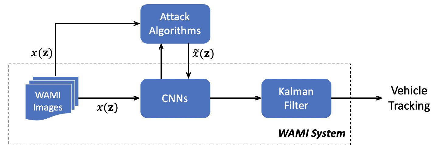
Figure 2: The Workflow of Attack on WAMI System.

The threat model of an adversary is summarised as in Figure 2. Assuming that $f_{N}(x(\mathbf{z}))=1$. An adversary must compute another input $\widetilde{x}(\mathbf{z})$ which requires a payoff and has a different classification, i.e., $f_{N}(\widetilde{x}(\mathbf{z}))=0$. Without loss of generality, the $\mathit{payoff}$ is measured with the norm-distance from $\widetilde{x}(\mathbf{z})$ to its original image $x(\mathbf{z})$, or formally

$$||\widetilde{x}(\mathbf{z})-x(\mathbf{z})||_{p}$$ (18)

To deviate from an input image $x(\mathbf{z})$ to its adversarial input $\widetilde{x}(\mathbf{z})$, a large body of adversarial example generation algorithms and adversarial test case generation algorithms are available. Given a neural network ${N}$ and an input $x$, an adversarial algorithm $A$ produces an adversarial example $A({N},x)$ such that $f_{N}(A({N},x))\neq f_{N}(x)$. On the other hand, for test case generation, an algorithm $A$ produces a set of test cases $A({N},x)$, among which the optimal adversarial test case is such that $\arg\min_{\widetilde{x}\in A({N},x),f_{N}(\widetilde{x})\neq f_{N}(x)}||\widetilde{x}-x||_{p}$. We remark that, the work in this paper is independent from particular adversarial algorithms. We use in our experiments two algorithms:

• DeepFool [40], which finds an adversarial example $\widetilde{x}$ by projecting $x$ onto the nearest decision boundary. The projection process is iterative because the decision boundary is non-linear.

• DeepConcolic [22], which generates a test suite by applying combined symbolic execution and concrete execution, guided by adapted MC/DC metrics for neural networks [24].

We denote by $\operatorname*{\mathit{payoff}}(A,{N},x)$, the payoff that an adversarial algorithm $A$ needs to compute for an adversarial example from $x$ and ${N}$. Furthermore, we assume that the adversary can observe the parameters of the Bayes filter, for example, $\mathbf{H}_{k},\mathbf{F}_{k}$, $\mathbf{Q}_{k},\mathbf{R}_{k}$ of the Kalman filter.

5.2 {PO}²-Labelled Transition Systems

Let $Prop$ be a set of atomic propositions. A payoff and partially-ordered label transition system, or {PO}²-LTS, is a tuple $M=(Q,q_{0},\operatorname*{\mathit{kf}},L,\pi,\beta)$, where $Q$ is a set of states, $q_{0}\in Q$ is an initial state, $\operatorname*{\mathit{kf}}\subseteq Q\times Q$ is a transition relation, $L:Q\rightarrow 2^{Prop}$ is a labelling function, $\pi:Q\times Q\rightarrow{}^{+}$ is a payoff function assigning every transition a non-negative real number, and $\beta:\operatorname*{\mathit{kf}}\rightarrow\operatorname*{\mathit{kf}}$ is a partial order relation between out-going transitions from the same state.

5.3 Reduction of WAMI Tracking to {PO}²-LTS

We model a neural network enabled state estimation system as a {PO}²-LTS. A brief summary of some key notations in this paper is provided in Table 1. We let each pair $(\mathbf{s}_{k},\mathbf{P}_{k})$ be a state, and use the transition relation $\operatorname*{\mathit{kf}}$ to model the transformation from a pair to another pair in a Bayes filter. We have the initial state $q_{0}$ by choosing a detected vehicle $(\mathbf{s}_{0},\mathbf{P}_{0})$ on the map. From a state $q_{k-1}=(\mathbf{s}_{k-1},\mathbf{P}_{k-1})$ and a set $Z_{k}$ of candidate observations, we have one transition $(q_{k-1},q_{k})$ for each $\mathbf{z}\in Z_{k}$, where $q_{k}=(\mathbf{s}_{k},\mathbf{P}_{k})$ can be computed with Equations (3)-(5) by having $\mathbf{z}_{k}$ in Equation (6) as the new observation. For a state $q_{k}=(\mathbf{s}_{k},\mathbf{P}_{k})$, we write $\mathbf{s}(q_{k})$ to denote the estimate $\mathbf{s}_{k}$, $\mathbf{P}(q_{k})$ to denote the covariance matrix $\mathbf{P}_{k}$, and $\mathbf{z}(q_{k})$ to denote the new observation that has been used to compute $\mathbf{s}(q_{k})$ and $\mathbf{P}(q_{k})$ from its parent state $q_{k-1}$.

Notations	Description
$\mathbf{z}_{k}\in Z_{k}$	observed location by WAMI tracking
$x(\mathbf{z})$	an $d_{1}$$\times$$d_{2}$ image covering location $\mathbf{z}$
$f_{N}$	neural network function
$\operatorname*{\mathit{payoff}}(A,{N},x)$	payoff for algorithm $A$ computing an adversarial example from $x$ and ${N}$
$q_{k}=(\mathbf{s}_{k},\mathbf{P}_{k})$	a state at step $k$, consisting of estimate and covariance matrix
$\mathbf{s}(q_{k})$, $\mathbf{P}(q_{k})$ and $\mathbf{z}(q_{k})$	estimate of $q_{k}$, covariance matrix of $q_{k}$ and observed location for transition $(q_{k-1},q_{k})$
$\rho$	a path of consecutive states $q_{l}...q_{u}$
$\rho_{k}$, $\mathbf{z}(\rho_{k})$	alias: the state $q_{k}$ and the observed location $\mathbf{z}(q_{k})$ on the path $\rho$

Table 1: A Summary of Notations Used

Subsequently, for each transition $(q_{k-1},q_{k})$, its associated payoff $\pi(q_{k-1},q_{k})$ is denoted by $\operatorname*{\mathit{payoff}}(A,{N},x(\mathbf{z}(q_{k})))$, i.e., the payoff that the adversary uses the algorithm $A$ to manipulate $x(\mathbf{z}(q_{k}))$ – the image covering the observation $\mathbf{z}(q_{k})$ – into another image on which the neural network ${N}$ believes there exists no vehicle.

For two transitions $(q_{k-1},q_{k}^{1})$ and $(q_{k-1},q_{k}^{2})$ from the same state $q_{k-1}$, we say that they have a partial order relation, written as $(q_{k-1},q_{k}^{1})\prec(q_{k-1},q_{k}^{2})$, if making $\mathbf{z}(q_{k}^{2})$ the new observation requires the adversary to fool the network ${N}$ into misclassifying $x(\mathbf{z}(q_{k}^{1}))$. For example, in WAMI tracking, according to Equation (6), the condition means that $||\mathbf{z}(q_{k}^{2})-\mathbf{z}||_{p}>||\mathbf{z}(q_{k}^{1})-\mathbf{z}||_{p}$, where $\mathbf{z}=\mathbf{H}_{k}\mathbf{s}(q_{k-1})$ is the predicted location.

Example 1

Figure 3 depicts a tree diagram for the unfolding of a labelled transition system. The root node on top represents the initial state $q_{0}$. Each layer comprises all possible states of $q_{k}=(\mathbf{s}_{k},\mathbf{P}_{k})$ at step $k$ of WAMI tracking, with $\mathbf{s}_{k}$ being one possible estimate, and $\mathbf{P}_{k}$ the covariance matrix. Each transition connects a state $q_{k-1}$ at step $k$$-$$1$ to $q_{k}$ at step $k$. $\dots,\mathbf{z}_{k},\mathbf{z}_{k+1},\mathbf{z}_{k+2},\dots$ are the observed locations at each step by WAMI tracking.

Given a {PO}²-LTS $M$, we define a path $\rho$ as a sequence of consecutive states $q_{l}...q_{u}$, and $\mathbf{z}(\rho)$ as a sequence of corresponding observed location $\mathbf{z}_{l}...\mathbf{z}_{u}$ for $0\leq l<u$, where $l$ and $u$ are the starting and ending time under consideration, respectively. We write $\rho_{k}$ for the state $q_{k}$, and $\mathbf{z}(\rho_{k})$ for the observed location $\mathbf{z}(q_{k})$ on the path $\rho$.

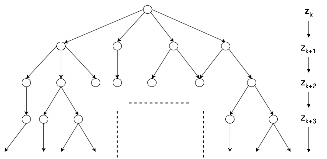
Figure 3: Tree diagram of an unfolding {PO}²-LTS

6 Property Specification: Robustness and Resilience

Formal verification determines whether a specification $\phi$ holds on a given LTS $M$ [41]. Usually, a logic language, such as CTL, LTL, or PCTL, is used to formally express the specification $\phi$. In this paper, to suit our needs, we let the specification $\phi$ be a constrained optimisation objective; and so verification is undertaken in two steps:

1. determine whether, given $M$ and $\phi$, there is a solution to the constrained optimisation problem. If the answer is affirmative, an optimal solution $sol_{opt}(M,\phi)$ is returned.

2. compare $sol_{opt}(M,\phi)$ with a pre-specified threshold $\theta$. If $sol_{opt}(M,\phi)>\theta$ then we say that the property $\phi$ holds on the model $M$ with respect to the threshold $\theta$. Otherwise, it fails.

Note that, we always take a minimisation objective in the first step. Since the optimisation is to find the minimal answer, in the second step, if $sol_{opt}(M,\phi)>\theta$, we cannot have a better – in terms of a smaller value – solution for the threshold $\theta$. Intuitively, it is a guarantee that no attacker can succeed with less cost than $\theta$, and the system is hence safe against the property. The above procedure can be easily adapted if we work with maximisation objectives.

Before proceeding to the formal definition of the robustness and resilience properties, we need several notations. First, we consider the measure for the loss of localisation precision. Let $\rho$ be an original path that has not suffered from an attack. The other path $\widetilde{\rho}$ is obtained after an attack on $\rho$. For the WAMI tracking system, we define their distance at time $k$ as

$$dist(\rho_{k},\widetilde{\rho}_{k})=||x(\mathbf{z}(\rho_{k}))-x(\mathbf{z}(\widetilde{\rho}_{k}))||_{p}$$ (19)

which is the $L^{p}$-norm difference between two images $x(\mathbf{z}(\rho_{k}))$ and $x(\mathbf{z}(\widetilde{\rho}_{k}))$.

Moreover, let $(\widetilde{\rho}_{k-1},\widetilde{\rho}_{k})$ be a transition on an attacked path $\widetilde{\rho}$, and so we have

$$\varphi(\widetilde{\rho}_{k-1},\widetilde{\rho}_{k})=\sum_{(\widetilde{\rho}_{k-1},\widetilde{\rho}_{k}^{\diamond})\prec(\widetilde{\rho}_{k-1},\widetilde{\rho}_{k})}\pi(\widetilde{\rho}_{k-1},\widetilde{\rho}_{k}^{\diamond})$$ (20)

as the combined payoffs that are required to implement the transition $(\widetilde{\rho}_{k-1},\widetilde{\rho}_{k})$. Intuitively, it requires that all the payoffs of the transitions $(\widetilde{\rho}_{k-1},\widetilde{\rho}_{k}^{\diamond})$, which are partially ordered by the envisaged transition $(\widetilde{\rho}_{k-1},\widetilde{\rho}_{k})$, are counted. In the WAMI tracking system, this means that the attack results in misclassifications of all the images $x(\mathbf{z}(\widetilde{\rho}_{k}^{\diamond}))$ such that the observation $\mathbf{z}(\widetilde{\rho}_{k}^{\diamond})$ is closer to the predicted location $\mathbf{F}_{k}\mathbf{s}(\widetilde{q}_{k-1})$ than $\mathbf{z}(\widetilde{\rho}_{k})$.

6.1 Definition of Robustness

Robustness is a concept that has been studied in many fields such as psychology [42], biomedical analysis [43], and chemical analysis [44]. Here, we adopt the general definition of robustness as used in the field of artificial intelligence (we later discuss the difference between this and the definition applied in software engineering):

Robustness is an enforced measure to represent a system’s ability to consistently deliver its expected functionality by accommodating disturbances to the input.

In LE-SESs, we measure the quality of the system maintaining its expected functionality under attack on a given scenario with the distance between two paths – its original path and the attacked path. Formally, given a track $\rho$ and an attacker, it is to consider the minimal perturbation to the input that can lead to misfunction. Intuitively, the larger the amount of perturbations a system can tolerate, the more robust it is. Let

$$dist^{0,e}(\rho,\widetilde{\rho})=\sum_{k=0}^{e}dist(\rho_{k},\widetilde{\rho}_{k})$$ (21)

be the accumulated distance, between the original track $\rho$ and the attacked track $\widetilde{\rho}$, from the start $k=0$ to the end $k=e$.

Moreover, we measure the disturbances to an LE-SES as the perturbation to its imagery input. Formally, we let

$$\varphi^{l,u}(\widetilde{\rho})=\sum_{k=l+1}^{u}\varphi(\widetilde{\rho}_{k-1},\widetilde{\rho}_{k})$$ (22)

be the accumulated combined payoff for the attacked track $\widetilde{\rho}$ between time steps $l$ and $u$, such that $l\geq 0$ and $u\leq e$. When $\varphi^{0,e}(\widetilde{\rho})=0$, there is no perturbation and $\widetilde{\rho}$ is the original track $\rho$.

Finally, we have the following optimisation objective for robustness:

$$\begin{array}[]{rl}\underset{\widetilde{\rho}}{\textbf{minimize}}&\varphi^{l,u}(\widetilde{\rho})\\ \textbf{subject to}&dist^{0,e}(\rho,\widetilde{\rho})>\epsilon_{robustness}\\ \end{array}$$ (23)

Basically, $\varphi^{l,u}(\widetilde{\rho})$ represents the amount of perturbation to the input, while the malfunctioning of system is formulated as $dist^{0,e}(\rho,\widetilde{\rho})>\epsilon_{robustness}$; that is, the deviation of the attacked track from the original track exceeds a given tolerance $\epsilon_{robustness}$.

6.2 Definition of Resilience

For resilience we take an ecological view widely seen in longitudinal population[45], psychological[46], and biosystem[47] studies.

Generally speaking, resilience indicates an innate capability to maintain or recover sufficient functionality in the face of challenging conditions [48] against risk or uncertainty, while keeping a certain level of vitality and prosperity [46].

This definition of resilience does not consider the presence of risk as a parameter [45], whereas the risks usually present themselves as uncertainty with heterogeneity in unpredictable directions including violence [49]. The outcome of the resilience is usually evidenced by either: a recovery of the partial functionality, albeit possibly with a deviation from its designated features [50]; or a synthetisation of other functionalities with its adaptivity in congenital structure or inbred nature. In the context of this paper, therefore resilience can be summarised as the system’s ability to continue operation (even with reduced functionality) and recover in the face of adversity. In this light, robustness, inter alia, is a feature of a resilient system. To avoid complicating discussions, we treat them separately.

In our definition, we take $dist^{e,e}(\rho,\widetilde{\rho})\leq\epsilon_{resilience}$ as the signal that the system has recovered to its designated functionality. Intuitively, $dist^{e,e}(\rho,\widetilde{\rho})\leq\epsilon_{resilience}$ means that the tracking has already returned back to normal – within acceptable deviation $\epsilon_{resilience}$ – on the time step $e\geq u$.

Moreover, we take

$$dist^{max}=\underset{t\in[l..u]}{\textbf{maximise}}~{}dist^{t,t}(\rho,\widetilde{\rho})$$ (24)

to denote the deviation of a path $\widetilde{\rho}$ from the normal path $\rho$. Intuitively, it considers the maximum distance between two locations – one on the original track and the other on the attacked track – of some time step $t$. The notation $max$ on $dist^{max}$ denotes the time step corresponding to the maximal value.

Then, the general idea of defining resilience for LE-SESs is that we measure the maximum deviation at some step $t\in[l,u]$ and want to know if the whole system can respond to the false information, gradually adjust itself, and eventually recover. Formally, taking $e\geq u$, we have the following formal definition of resilience:

$$\begin{array}[]{rl}\underset{\widetilde{\rho}}{\textbf{minimise}}&dist^{max}\\ \textbf{subject to}&dist^{e,e}(\rho,\widetilde{\rho})>\epsilon_{resilience}\end{array}$$ (25)

Intuitively, the general optimisation objective is to minimize the maximum deviation such that the system cannot recover at the end of the track. In other words, the time $e$ represents the end of the track, where the tracking functionality should have recovered to a certain level – subject to the loss $\epsilon_{resilience}$.

We remark that, for resilience, the definition of “recovery” can be varied. While in Equation (25) we use $dist^{e,e}(\rho,\widetilde{\rho})\leq\epsilon_{resilience}$ to denote the success of a recovery, there can be other definitions, for example, asking for a return to some track that does not necessarily have be the original one, so long as it is acceptable.

6.3 Computational Complexity

We study the complexity of the {PO}²-LTS verification problem and show that the problem is NP-complete for robustness. Concretely, for the soundness, an adversary can take a non-deterministic algorithm to choose the states $\hat{\rho}_{k}$ for a linear number of steps, and check whether the constraints satisfy in linear time. Therefore, the problem is in NP. To show the NP-hardness, we reduce the knapsack problem – a known NP-complete problem – to the same constrained optimisation problem as Equation (23) on a {PO}²-LTS.

The general Knapsack problem is to determine, given a set of items, each with a weight and a value, the number of each item to include in a collection so that the total weight is less than or equal to a given limit, and the total value is as large as possible. We consider 0-1 Knapsack problem, which restricts the number $c_{i}$ of copies of each kind of item to zero or one. Given a set of $n$ items numbered from 1 up to $n$, each with a weight $g_{i}$ and a value $v_{i}$, along with a maximum weight $W$, the aim is to compute

$$\underset{}{\textbf{maximise}}{}{} \sum_{i=1}^{n}v_{i}c_{i}$$ (26)

subject to $$\sum_{i=1}^{n}g_{i}c_{i}\leq W$$

$$\forall i\in[1..n]:c_{i}\in\{0,1\}$$

where $c_{i}$ represents the number of the item $i$ to be included in the knapsack. Informally, the problem is to maximize the sum of the values of the items in the knapsack so that the sum of the weights is less than or equal to the knapsack’s capacity.

We can construct a {PO}²-LTS $M=(Q,q_{0},\operatorname*{\mathit{kf}},L,\pi,\beta)$, where $Q=\{q_{0}\}\cup\bigcup_{i=1}^{n}\{q_{i0},q_{i1}\}$. Intuitively, for every item $i$, we have two states representing whether or not the item is selected, respectively. For the transition relation $\operatorname*{\mathit{kf}}$, we have that $\operatorname*{\mathit{kf}}=\{(q_{0},q_{1j})|j\in\{0,1\}\}\cup\{(q_{ij},q_{(i+1)j^{\prime}})|i\in\{1..n-1\},j,j^{\prime}\in\{0,1\}\}$, which connects each state of item $i$ to the states of the next item $i+1$. The payoff function $\pi$ is defined as $\pi(q,q_{i0})=0$ and $\pi(q,q_{i1})=v_{i}$, for all $(q,q_{ij})\in\operatorname*{\mathit{kf}}$ and $j\in\{0,1\}$, representing that it will take $v_{i}$ payoff to take the transition $(q,q_{i1})$ in order to add the item $i$ into the knapsack, and take $0$ payoff to take the other transition $(q,q_{i0})$ in order to not add the item $i$. The partial order relation $\beta$ can be defined as having transition $(q,q_{i0})\prec(q,q_{i1})$, for all $(q,q_{ij})\in\operatorname*{\mathit{kf}}$ and $j\in\{0,1\}$.

For the specification, we have the following robustness-related optimisation objective.

$$\begin{array}[]{rl}\underset{\widetilde{\rho}}{\textbf{minimize}}&\varphi^{1,n}(\widetilde{\rho})\\ \textbf{subject to}&dist^{1,n}(\rho,\widetilde{\rho})>W\\ \end{array}$$ (27)

such that

$$dist(\rho_{k},\widetilde{\rho}_{k})=\left\{\begin{array}[]{ll}0&\text{ if }\widetilde{\rho}_{k}=q_{k0}\\ g_{k}&\text{ if }\widetilde{\rho}_{k}=q_{k1}\end{array}\right.$$ (28)

Recall that, $\varphi^{1,n}(\widetilde{\rho})$ is defined in Equations (22) and (20), and $dist^{1,n}(\rho,\widetilde{\rho})$ is defined in Equation (21). As a result, the robustness of the model $M$ and the above robustness property is equivalent to the existence of a solution to the 0-1 Knapsack problem. This implies that the robustness problem on {PO}²-LTSs is NP-complete.

7 Automated Verification Algorithm

An attack on the LE-SESs, as explained in Section 5.1, adds perturbations to the input images in order to fool a neural network, which is part of the perception unit, into making wrong detections. On one hand, these wrong detections will be passed on to the perception unit, which in turn affects the Bayes filter and leads to wrong state estimation; the LE-SES can be vulnerable to such attack. On the other hand, the LE-SESs may have internal or external mechanisms to tolerate such attack, and therefore perform well with respect to properties such as robustness or resilience. It is important to have a formal, principled analysis to understand how good a LE-SES is with respect to the properties and whether a designed mechanism is helpful in improving its performance.

We have introduced in Section 5 how to reduce an LE-SES into a {PO}²-LTS $M$ and formally express a property – either robustness or resilience – with a constrained optimisation objective $\phi$ based on a path $\rho$ in Section 6. Thanks to this formalism, the verification of robustness and resilience can be outlined using the same algorithm. Now, given a model $M$, an optimisation objective $\phi$, and a pre-specified threshold $\theta$, we aim to develop an automated verification algorithm to check whether the model $M$ is robust or resilient on the path $\rho$; or formally, $sol_{opt}(M,\phi)>\theta$, where $sol_{opt}(M,\phi)$ denotes the optimal value obtained from the constrained optimisation problem over $M$ and $\phi$.

The general idea of our verification algorithm is as follows. It first enumerates all possible paths of $M$ obtainable by attacking the given path $\rho$ (Algorithm 1), and then determines the optimal solution $sol_{opt}(M,\phi)$ among the paths (Algorithm 2). Finally, the satisfiability of the property is determined by comparing $sol_{opt}(M,\phi)$ and $\theta$.

7.1 Exhaustive Search for All Possible Tracks

The first step of the algorithm proceeds by exhaustively enumerating all possible attacked paths on the {PO}²-LTS $M$ with respect to $\rho$. It is not hard to see that, the paths will form a tree, unfolded from the {PO}²-LTS $M$, as illustrated in Figure 3. Since a final deviation is not available until the end of a simulation, the tree has to be fully expanded from the root to the leaf and all the paths explored. Clearly, the time complexity of this procedure is exponential with respect to the number of steps, which is consistent with our complexity result, as presented in Section 6.3. Specifically, breadth-first search (BFS) is used to enumerate the paths. The details are presented in Algorithm 1.

0:  LTS model $M$, $n$, $l$, $u$

0:  path set $P$, payoff set $\varphi^{l,u}$

1:  run original path $\rho$ from $k=0$ to $k=n$

2:  set $\rho_{l-1}$ as root node

3:  for $k$ from $l$$-$$1$ to $u$ do

4:     for each node $\widetilde{\rho}_{k}$ in $leaf(\rho_{l-1})$ do

5:        find potential observations $Z\leftarrow neighbours(\widetilde{\rho}_{k})$

6:        for each observed location $\mathbf{z}$ in $Z$ do

7:           $\widetilde{\rho}_{k+1}\leftarrow kf(\widetilde{\rho}_{k},\mathbf{z})$

8:           calculate the attack payoff $\varphi(\widetilde{\rho}_{k+1},\widetilde{\rho}_{k})$

9:           $\widetilde{\rho}_{k}=parent(\widetilde{\rho}_{k+1})$

10:        end for

11:     end for

12:  end for

13:  $P\leftarrow path(\rho_{l-1})$

14:  run path $\widetilde{\rho}$ in set $P$ to $k=n$

15:  calculate the combined payoff for each path $\widetilde{\rho}$ $\varphi^{l,u}(\widetilde{\rho})=\sum_{k=l}^{u}\varphi(\widetilde{\rho}_{k-1},\widetilde{\rho}_{k})/(u-l)$

16:  return  $P$, $\varphi^{l,u}$

Algorithm 1 Exhaustive Search based on BFS

We need several operation functions on the tree, including $leaf$ (which returns all leaf nodes of the root node), $parent$ (which associates a node to its parent node), and $path$ (which returns all tree paths from the given root node to the leaf nodes).

Lines 2-12 in Algorithm 1 present the procedure of constructing the tree diagram. First, we set the root node $\rho_{l-1}$ (Line 2), that is, we will attack the system from the ($l$$-$$1$)-th state of the original track $\rho$ and enumerate all possible adversarial tracks. At each step $k$, function $neighbours$ will list all observations near the predicted location (Line 5). Then, each observation is incorporated with current state $\mathbf{\rho}_{k}$ for the calculation of the next state $\mathbf{\rho}_{k+1}$ (Line 7). If no observation is available or $z=\emptyset$ , the KF can still run normally, skipping the update phase. To enable each transition $(\mathbf{\rho}_{k},\mathbf{\rho}_{k+1})$, the partial order relation is followed when attacking the system and recording the payoff $\varphi$ (Line 8). Then, the potential $\mathbf{\rho}_{k+1}$ is accepted and added as the child node of $\mathbf{\rho}_{k}$. Once the tree is constructed, we continue simulating the tracks to the end of time, $k=n$, (Lines 13-14). Finally, all the paths in set $P$ are output along with the attack payoff $\varphi^{l,u}$ (Lines 15-16).

7.2 Computing an Optimal Solution to the Constrained Optimisation Problem

After enumerating all possible paths in $P$, we can compute optimal solutions to the constrained optimisation problems as in Equation (23) and (25). We let $obj$ be the objective function to minimize, and $con$ be the constraints to follow. For robustness, we have $obj=\varphi^{l,u}$ and $con=dist^{0,e}$, and for resilience, we have $obj=dist^{max}$ and $con=dist^{e,e}$.

0:  path set $P$, $obj$, $con$, $\epsilon$

0:  representative path $\widetilde{\rho}^{*}$, $obj$ value $\theta^{*}$ of $\rho^{*}$, and optimal value $sol_{opt}(M,\phi)$

1:  find the original path $\rho$ in set $P$

2:  $sol_{opt}(M,\phi)\leftarrow 0$, $k\leftarrow 0$, $P^{+}\leftarrow\emptyset$, $P^{-}\leftarrow\emptyset$

3:  for $\widetilde{\rho}$ in set $P$ do

4:     if $con(\rho,\widetilde{\rho})>\epsilon$ then

5:        $k\leftarrow k+1$

6:        $P^{+}\leftarrow P^{+}\cap\{\widetilde{\rho}\}$

7:        if $k=1$ or $obj(\rho,\widetilde{\rho})<sol_{opt}(M,\phi)$ then

8:           $sol_{opt}(M,\phi)\leftarrow obj(\rho,\widetilde{\rho})$

9:        end if

10:     else

11:        $P^{-}\leftarrow P^{-}\cap\{\widetilde{\rho}\}$

12:     end if

13:  end for

14:  $\rho^{*}\leftarrow\arg\max_{\widetilde{\rho}\in P^{-},obj<sol_{opt}(M,\phi)}obj(\rho,\widetilde{\rho})$

15:  $\theta^{*}\leftarrow obj(\rho,\rho^{*})$

16:  return  $\rho^{*}$, $\theta^{*}$, $sol_{opt}(M,\phi)$

Algorithm 2 Computation of Optimal Solution and A Representative Path

Note that, our definitions in Equations (23) and (25) are set to work with cases that do not satisfy the properties, i.e., paths that are not robust or resilient, and identify the optimal one from them. Therefore, a path satisfying the constraints suggests that it does not satisfy the property. We split the set $P$ of paths into two subsets, $P^{+}$ and $P^{-}$. Intuitively, $P^{+}$ includes those paths satisfying the constraints, i.e., fail to perform well with respect to the property, and $P^{-}$ includes those paths that do not satisfy the constraints, i.e., perform well with respect to the property. For robustness, $P^{+}$ includes paths satisfying $dist^{0,e}(\rho,\widetilde{\rho})>\epsilon$ and $P^{-}$ satisfying $dist^{0,e}(\rho,\widetilde{\rho})\leq\epsilon$. For resilience, $P^{+}$ includes paths satisfying $dist^{e,e}(\rho,\widetilde{\rho})>\epsilon$ and $P^{-}$ satisfying $dist^{e,e}(\rho,\widetilde{\rho})\leq\epsilon$.

In addition to the optimal solutions that, according to the optimisation objectives, are some of the paths in $P^{+}$, it is useful to identify certain paths in $P^{-}$ that are robust or resilient. Let $sol_{opt}(M,\phi)$ be the optimal $obj$ value, from the optimal solution. We can sort the paths in $P^{-}$ according to their $obj$ value, and let representative path $\rho^{*}$ be the path whose $obj$ value is the greatest among those smaller than $sol_{opt}(M,\phi)$. Intuitively, $\rho^{*}$ represents the path that is closest to the optimal solution of the optimisation problem but satisfies the corresponding robust/resilient property. This path is representative because it serves as the worst case scenario for us to exercise the system’s robust property and resilient property respectively. Moreover, we let $\theta^{*}$ be the $obj$ value of robustness/resilience of the path $\rho^{*}$, called representative value in the paper.

The algorithm for the computation of the optimal solution and a representative path can be found in Algorithm 2. Lines 1 to 9 give the process to solve Equation (23) or (25) for the optimal value $sol_{opt}(M,\phi)$. The remaining Lines calculate the representative value $\theta^{*}$ and a representative path $\rho^{*}$.

For each adversarial path in $P$, it is added into either $P^{+}$ (Line 6) or $P^{-}$ (Line 11). The minimum objective function is then found by comparing the adversarial tracks in set $P^{+}$ (Lines 4-9). We need to find the representative path in set $P^{-}$, which has the $obj$ value smaller than $sol_{opt}(M,\phi)$ but lager than any other path in $P^{-}$ (Line 14). Its corresponding representative value is computed in Line 15.

8 Experimental Results

We conduct an extensive set of experiments to show the effectiveness of our verification algorithm in the design of the WAMI tracking system. We believe that our approaches can be easily generalised to work with other autonomous systems using both Bayes filter(s) and neural networks.

8.1 Research Questions

Our evaluation experiments are guided by the following research questions.

• What is the evidence of system level robustness and resilience for the WAMI tracking in Section 3?

• What are the differences and similarity between robustness and resilience within the WAMI tracking?

• Following RQ1 and RQ2, can our verification approach be used to identify, and quantify, the risk to the robustness and resilience of the WAMI tracking system?

• Are the improved design presented in Section 4 helpful in improving the system’s robustness and resilience?

Their respective experiments and results are presented in Section 8.3, 8.4, 8.5 and 8.6.

8.2 Experimental Setup

We consider a number of original tracks with maximum length of 20 steps ($e=19,k\in[0,19]$). An attack on the system is conducted between time steps $l$ and $u$, denoted as $Attack(l,u)$, with the following configurations: $l\in[4,12]$, and $(u-l)\in[1,4]$. The original track is coloured in green in both the high-resolution images (Figure 4–10) and the state space unfolding (Figure 7(c)). The attacked track is coloured in red. The white-colour arrows in the high-resolution images indicate the ground-truth directions of the vehicle.

Moreover, in all experiments, for every attacked track, we record the following measures: the combined payoff $\varphi$, the cumulative deviation $dist^{0,e}$, the maximum deviation $dist^{max}$ and the final step deviation $dist^{e,e}$, such that $m$ is the time step for maximum deviation and $e$ is the end of the track.

8.3 Evidence of System’s Robustness and Resilience

To demonstrate the system’s robustness and resilience against the perturbance on its imagery input, we show the attack on the WAMI tracking in Figure 4(a) with combined payoff $\varphi=10.47$. The payoff is calculated as the total perturbations added to the input images for generating the current adversarial track (coloured in red) against the original track (coloured in green). If we loosen the restriction on the attacker, for example, the attack payoff is increased to $\varphi=20.58$, with other settings remaining unchanged, we get the results in Figure 4(b). While the attacker’s effort is almost doubled (from $\varphi=10.47$ to $\varphi=20.58$), the deviation from the original track is not increased that much. This is evidence of the system level robustness. To have a better understanding about this, we investigate the updating process for tracking at $k=6$ and visualise the process in Figure 4(c) and 4(d) respectively.

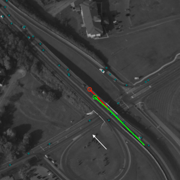
(a) $k=6$, $\varphi=10.47$

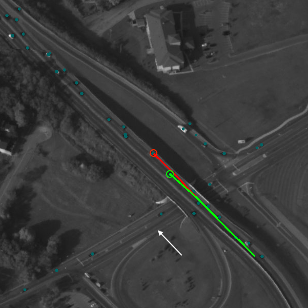
(b) $k=6$, $\varphi=20.58$

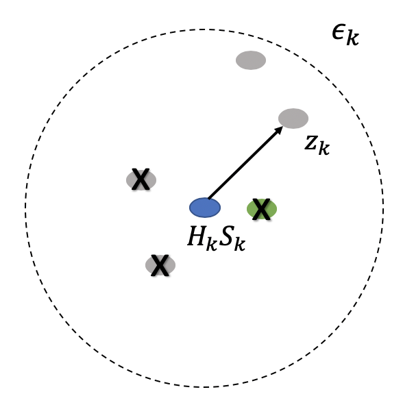
(c) KF’s update process for (a)

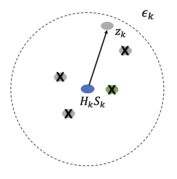
(d) KF’s update process for (b)

Figure 4: Illustration of WAMI system’s robustness to the consecutive attack at $k=5-6$. With increased attack payoff, the deviation is still bounded.

As shown in the Figure 4(c) and 4(d), the blue point identifies the predicted location of the tracking vehicle, the green point is the correct observation, and other grey points are observations of other vehicles around the tracked one. Other vehicles are potential disturbances to the system. For Scene (a), the attacker makes the closest three detections invisible to the system with an attack payoff $\varphi=10.47$. For scene (b), one more observation is mis-detected with the payoff increased to $\varphi=20.58$, and thus the KF associates the most distant observation as the observation for updating. Nevertheless, for both scenes, the wrong observations are still within the bound, which is denoted by the dashed circle.

We can see that the WAMI tracking system is designed in a way to be robust against the local disturbances. First, as presented in its architecture by Figure 1, the background subtraction can guarantee that only moving objects are input to the CNNs for vehicle detection; this means that error observations that can influence the tracking accuracy are discrete and finite, which are easier to control and measure than continuous errors. Second, the KF’s covariance matrix leads to a search range, only within which the observations are considered. In other words, even if the attacker has infinite power – measured as payoff – to attack the system at some step, the possible deviations can be enumerated and constrained within a known bound.

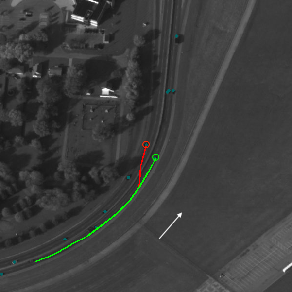
(a) vehicle tracking at $k=9$

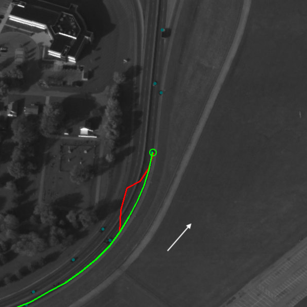
(b) vehicle tracking at $k=12$

Figure 5: Illustration of WAMI system’s resilience to the one step attack at $k=8$. The attack payoff $\varphi=6.49$.

To show the system’s resilience to erroneous behaviours, we consider the maximum deviation depicted in Figure 5(a), which arises from a one-step attack at $k=8$. After three steps forward, i.e., $k=12$, we have the tracking results as depicted in Figure 5(b). Evident in this test scene, the adversarial tracking is corrected by the system itself, back to the original expected track in a short time period – a clear evidence of resilience.

Taking a careful look into Figure 5(a), we can see that, at $k=8$, the attacked track is associated with a wrong observation in the opposite lane. Due to the consistency in the KF, this false information may disturb the original tracking, but cannot completely change some key values of the KF’s state variables; for example, the direction of the velocity vector. That means that, even for the adversarial tracking, the prediction still advances in the same direction to the previous one. Hence, this wrong observation will not appear in the search range of its next step. For this reason, it is likely that the tracking can be compensated and returned to the original target vehicle.

Another key fact is that, the KF’s covariance matrix will adjust according to the detection of observations. If no observation is available within the search range, the uncertainty range – decided by covariance matrix – will enlarge and very likely, the error tracking can be corrected. This reflects the KF’s good adaption to the errors – another key ability in achieving resilience.

We have the following takeaway message to RQ1:

The WAMI tracking system in Section 3.6 is robust and resilient (to some extent) against the adversarial attacks on its neural network perceptional unit.

8.4 Comparison Between Robustness and Resilience

Robustness and resilience as defined in Section 6 are both measures of a system’s capacity to handle perturbations; however, they are not equivalent definitions. To assist in appreciating the distinction, Figure 6 provides examples.

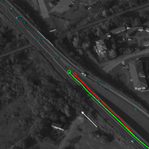
(a) robustness

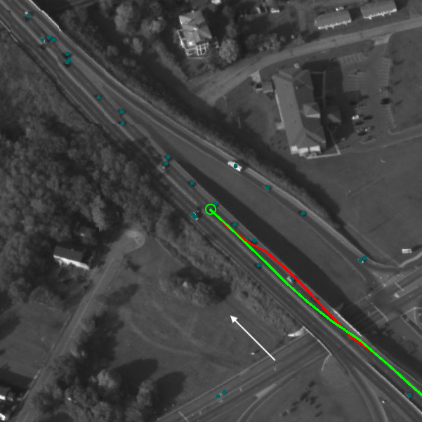
(b) resilience

(c) deviation of robust track

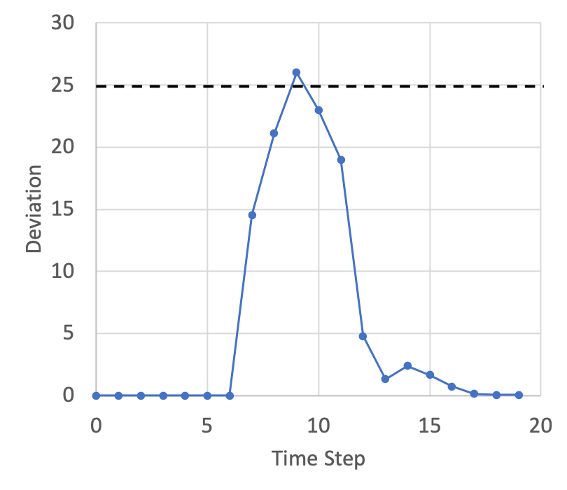
(d) deviation of resilient track

Figure 6: Comparison between robustness and resilience in WAMI tracking

In Figure 6, we present two typical cases to illustrate a system’s robustness and resilience against the attack. Their deviations from the original tracks at each step are recorded in Figure 6(c) and Figure 6(d), respectively. The horizontal dash line can be seen as the enhanced robustness threshold, requiring that each step’s deviation is smaller than some given threshold. For the vehicle tracking in Figure 6(a), we can say the system satisfies the robustness property against the disturbance, since the deviation at each step is bounded. However, this tracking is not resilient to the errors due to the loss of “recovery” property: it is apparent to see the deviation worsens over time. In contrast, for the vehicle tracking in Figure 6(b), the tracking is finally corrected – with the tracking back to the original track – at the end even when the maximum deviation (at time step 9) exceeds the robustness threshold. Therefore, to conclude, this vehicle tracking is resilient but not robust.

We have the following takeaway message to RQ2:

Robustness and resilience are different concepts and may complement each other in describing the system’s resistance and adaption to the malicious attack.

8.5 Quantify the Robustness and Resilience Bound

In the previous subsections, we have provided several examples to show the WAMI tracking system’s robustness and resilience to malicious attack. However, we still do not know to what extent the system is robust or resilient to natural environmental perturbation. In this subsection, we will show, from the verification perspective, a quantification of robustness and resilience of the WAMI tracking design in Section 3. That is, given an original track and its associated scene, whether or not we can quantify the robustness and resilience of that track, by solving the optimisation problem defined in Equation (23) and (25). Moreover, as quantitative measures rather than the optimal solutions, we will further get the representative path and representative value – as defined in Section 7.2 – of the tracking.

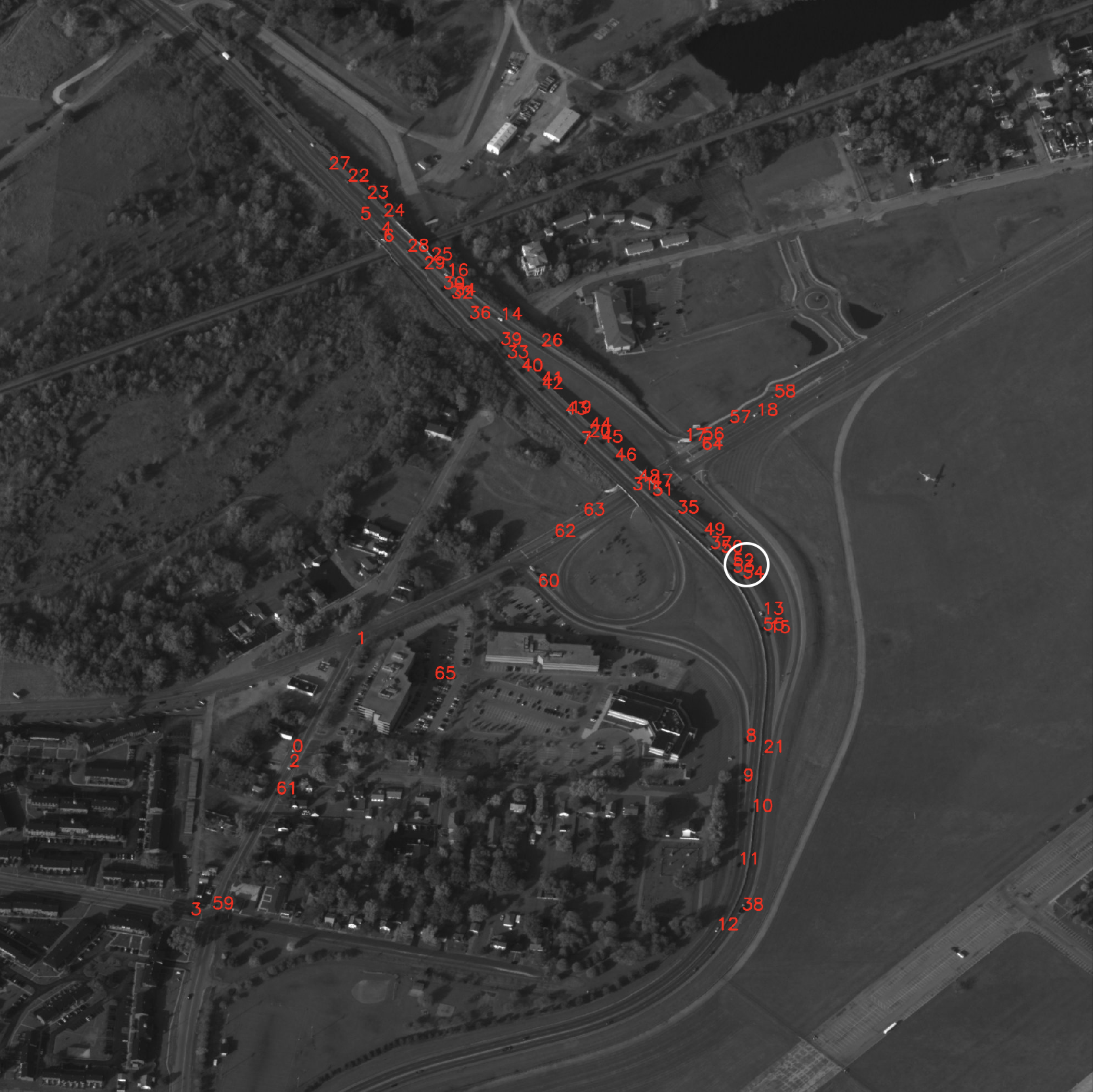
(a) test scene

(b) original track

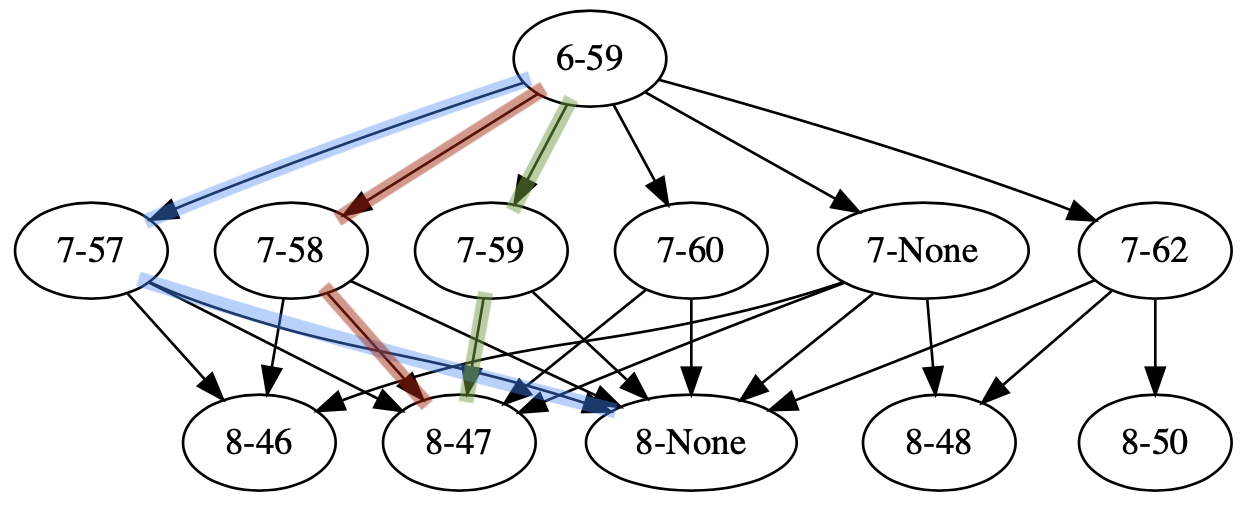
(c) Enumeration of all possible Tracks

Figure 7: Attack the system at $k=6,7,8$ on a selected scene. Tree graph exhibits all possible tracks, where green is the original track, blue is the resilience representative track, and red is the robustness representation track. The labels on the nodes represent “(time step)-(ID of associated detection)”.

Let us consider a track and the running test scene as shown in Figure 7. The white circle in Figure 7(a) contains the target vehicle and the green line in Figure 7(b) is the output of original tracking . By attacking the original track from time step $k=6$ to $k=8$, we can enumerate all the possible variants (using Algorithm 1) in Figure 7(c).

Table 2: Measures of all possible tracks for test scene in Figure 7: $\varphi$ is the combined payoff; $dist^{0,e}$, $dist^{max}$ and $dist^{e,e}$ are accumulated deviation, maximum deviation and end-point deviation between the original track $\rho$ and the adversarial track $\widetilde{\rho}$ respectively.

Track No.	1	2	3	4	5	6	7	8	9	10	11	12	13	14	15	16	17
$\varphi$	20.32	19.44	12.63	20.15	20.01	12.56	13.27	10.62	9.91	3.10	6.81	0.00	18.53	11.72	12.61	11.65	11.82
$dist^{0,e}$	529.99	103.17	7.23	5447.39	138.59	138.37	50.95	20.54	115.58	24.75	530.24	0.00	58.47	38.89	5462.11	5467.95	2430.17
$dist^{max}$	53.65	26.62	4.42	936.97	30.51	29.91	29.91	14.53	26.05	14.53	53.65	0.00	27.44	22.83	936.97	936.98	220.95
$dist^{e,e}$	53.65	0.07	0.01	936.97	0.06	0.06	0.01	0.01	0.06	0.01	53.65	0.00	0.01	0.01	936.97	936.98	210.13

To find the representative value, we record all the measures for each possible track in Table 2. Note that the attack payoff is calculated as the minimum perturbation for the current deviation, since we use the best attack approach, for example, Deepfool to find the shortest distance to the decision boundary in input space. Empirical parameters are set, e.g., like the robustness threshold $\epsilon_{robustness}=120$ (i.e., the system is robust if the cumulative deviation of 20 time steps does not exceed 120), and the resilience threshold $\epsilon_{resilience}=1$ (i.e., the system is resilient if the final deviation does not exceed 1). We remark that, these two hyper-parameters can be customised according to users’ particular needs.

Table 3: The outcome of robustness and resilience verification for test scene in Figure 7: $sol_{opt}(M,\phi)$ is the optimal value; $\theta^{*}$ and $\rho^{*}$ represents the representative value and track (of the robustness and the resilience) respectively.

	Robustness Verification	Resilience Verification
$sol_{opt}(M,\phi)$	6.81	53.65
$\theta^{*}$	3.10	30.51
$\rho^{*}$	colored in red (Figure 7(c))	colored in blue (Figure 7(c))

We then apply Algorithm 2 to search for the optimal solution to robustness and resilience verification, as defined in Equation (23) and (25). The verification outcome is presented in Table 3. The results show that optimal solution $sol_{opt}(M,\phi)$ to robustness verification is $\varphi=6.81$; the minimum attack payoff to lead to the failure of the system. The attack payoff $\varphi$ of Track No.11 and No.15 is greater or equal to $sol_{opt}(M,\phi)$, and have $dist^{0,e}$ over the robustness threshold. The result of resilience verification is $dist^{max}=53.65$, the minimum maximum deviation from which the system cannot recover. For example, the maximum deviation $dist^{max}$ of Track No.1 and No.15 is greater or equal to $sol_{opt}(M,\phi)$, and have $dist^{e,e}$ over the resilience threshold.

Moreover, we are interested in three specific tracks: (1) the original track, denoted as Track No. 12; (2) an adversarial track to represent the system’s robustness, denoted as Track No. 10; and (3) an adversarial track to represent the system’s resilience, denoted as Track No. 5. We can see that, the robustness representative value of the tracking is $\varphi=3.10$. If the attack payoff is constrained within this bound (including the bound value), the tracking of interest can have a guaranteed accumulative deviation smaller than 120. In addition, the resilience representative value is $dist^{max}=30.51$. If the defender can monitor the tracking and control the maximum deviation to make it smaller than or equal to this bound, the system can resist the errors and recover from the misfunction. These two tracks, reflecting the robustness and resilience respectively, are also plotted in Figure 8.

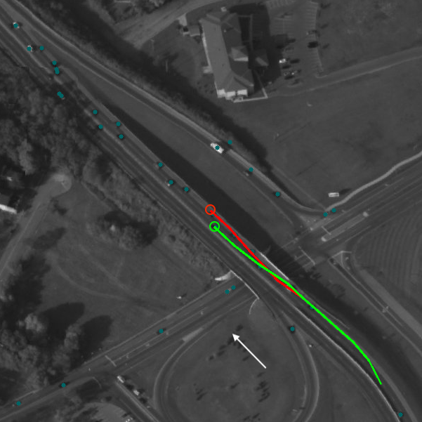
(a) robustness
representative track

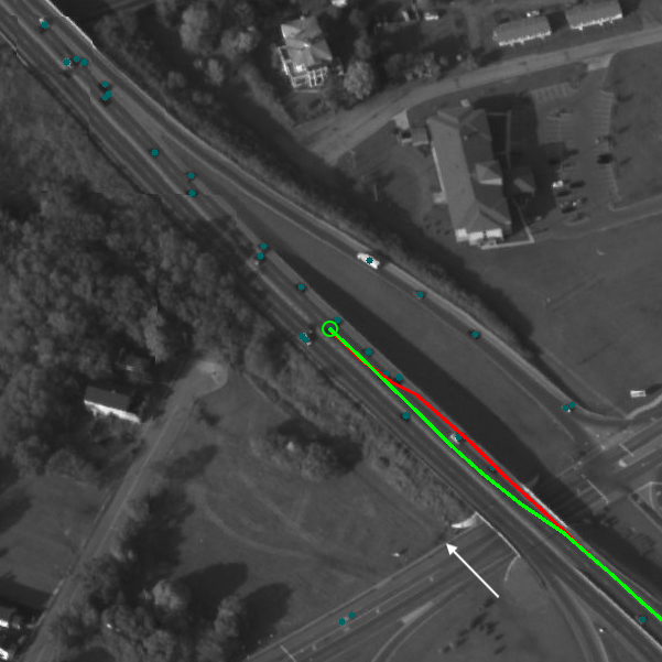
(b) resilience
representative track

Figure 8: Adversarial tracks to quantify the system’s robustness and resilience

Additionally, Table 2 also provides some other interesting observations that are worth discussing. For example, comparing Track No. 9, Track No.15 and Track No.16, it’s not difficult to determine that the deviation is very likely to increase dramatically when disturbances go over the system’s endurance. Under such circumstances, the maximum deviation normally occurs at the end of the tracking. In other words, the deviation will be increased further and further with time, and the KF is totally misled, such that it tracks other vehicles, distinctly distant to the intended one.

We have the following takeaway message to RQ3:

Our verification approach can not only find the optimal values for the optimisation problems as specified in (23) and Equation (25), but also find representative values and paths as defined in Section 7.2 to exhibit and quantify the robustness and resilience.

8.6 Improvement to the robustness and resilience

In this part, we apply the runtime monitor and the Joint KFs introduced in Section 4. We report whether theses two techniques can make an improvement to the WAMI tracking system through the experiments.

In Figure 9, a runtime monitor runs along with the system in order to continuously check the Bayesian uncertainty of the KF. As discussed in Section 4.1, a KF alternates between the prediction phase and the update phase, and the Bayesian uncertainty is gradually reduced until convergence. This can be seen from Figure 9(a) (Right), where there is no adversarial attack on the detection component and the uncertainty curve is very smooth. However, if the system is under attack, it is likely that the expected functionality of the KF is disrupted, and the KF performs in an unstable circumstance. Consequently, there will be time steps where no observations are available, leading to the increasing of uncertainty. When it comes to the uncertainty curve, as shown in Figure 9(b) (Right), a spike is observed.

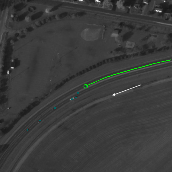
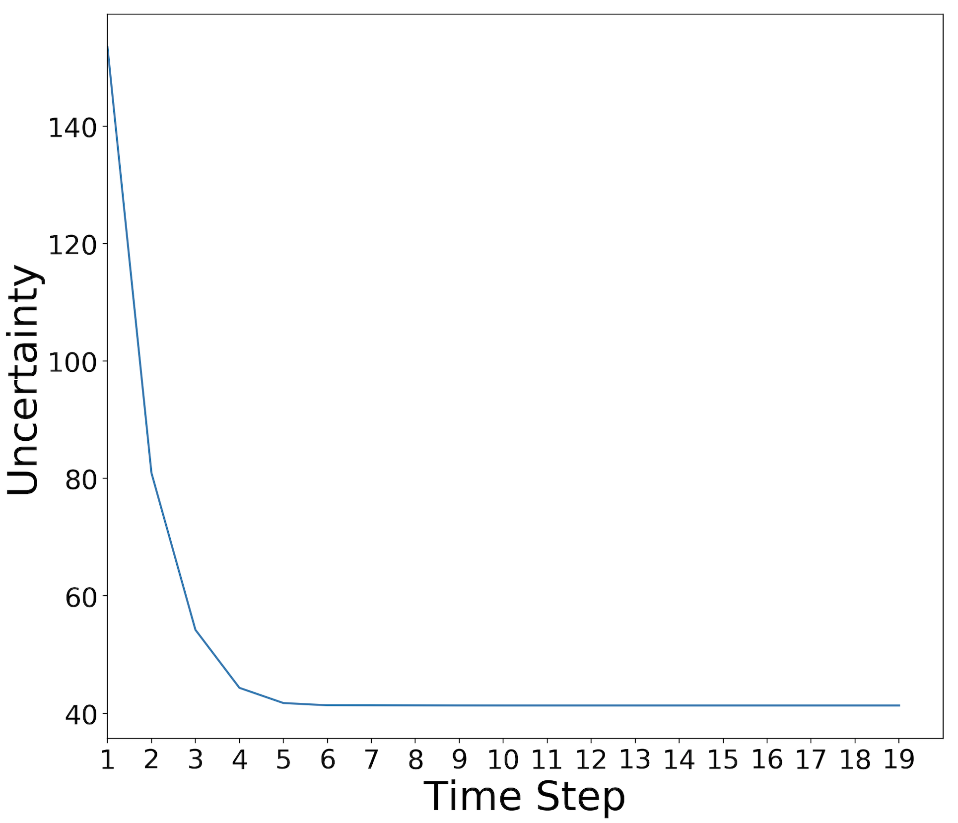
(a) tracking without attack

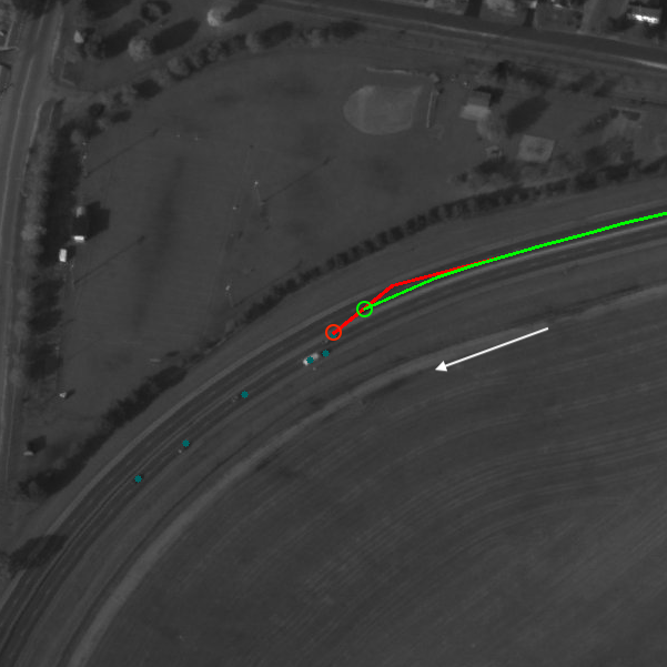
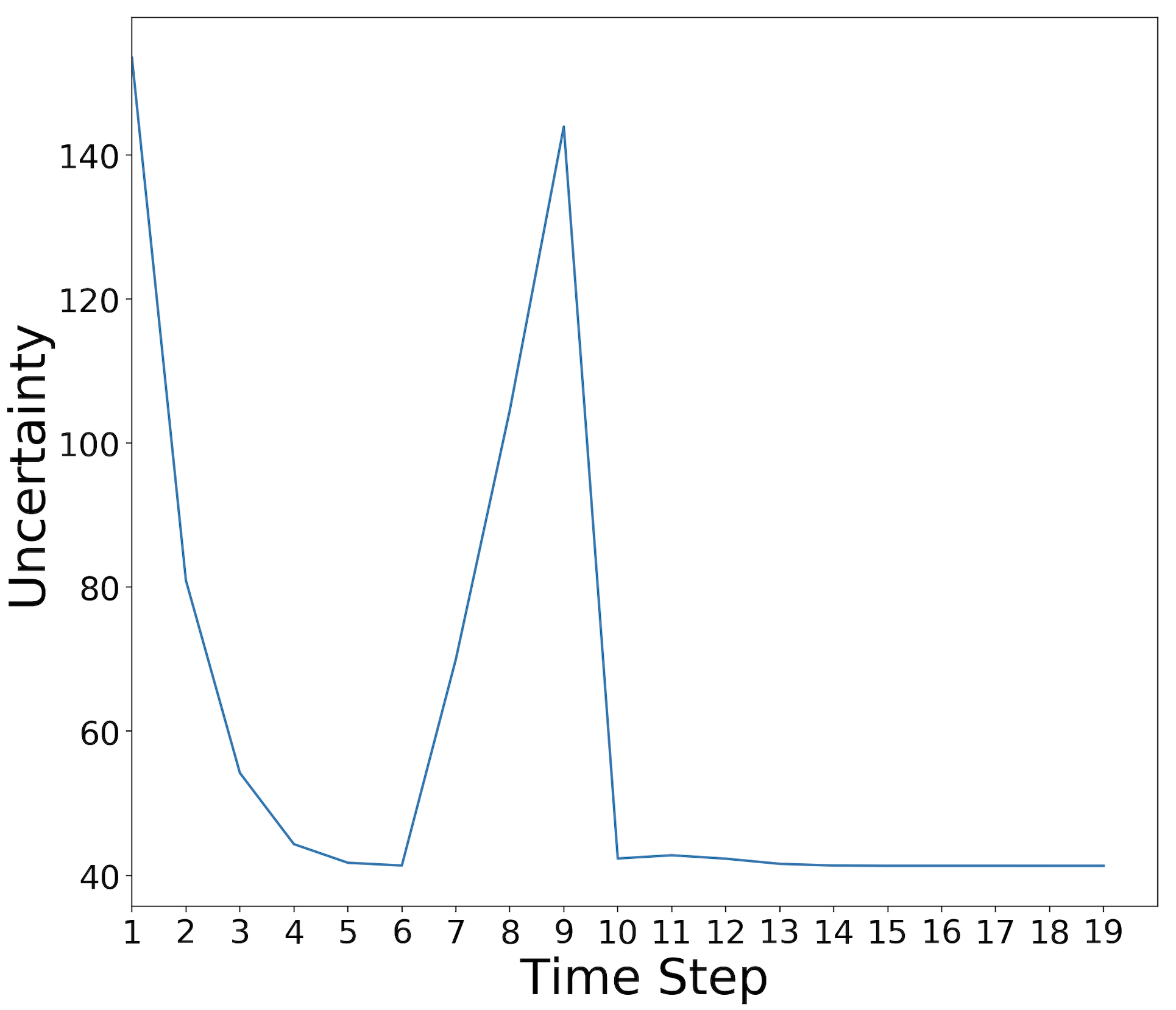
(b) tracking with attack

Figure 9: Runtime monitoring on the WAMI system’s tracking

The above discussion on uncertainty monitoring in Figure 9 is based on the condition that the environmental input is not complex and the surrounding vehicles are sparse: the mis-detection of vehicles is very likely to result in no observations seen by the system within the search range. For more complicated cases such that there are a significant number of vehicles in the input imagery, and the target tracking is more likely to be influenced by the surroundings, we need to refer to the improved design of taking joint-KFs for observation association filters in Section 4.2.

The main idea of implementing joint-KFs is to assign a tracking to each surrounding vehicle and the observation association is based on the maximum likelihood function as defined. In other words, if some surrounding vehicle has already been tracked by another KF, it will not be followed by the tracking of the current KF. An example is shown in Figure 10.

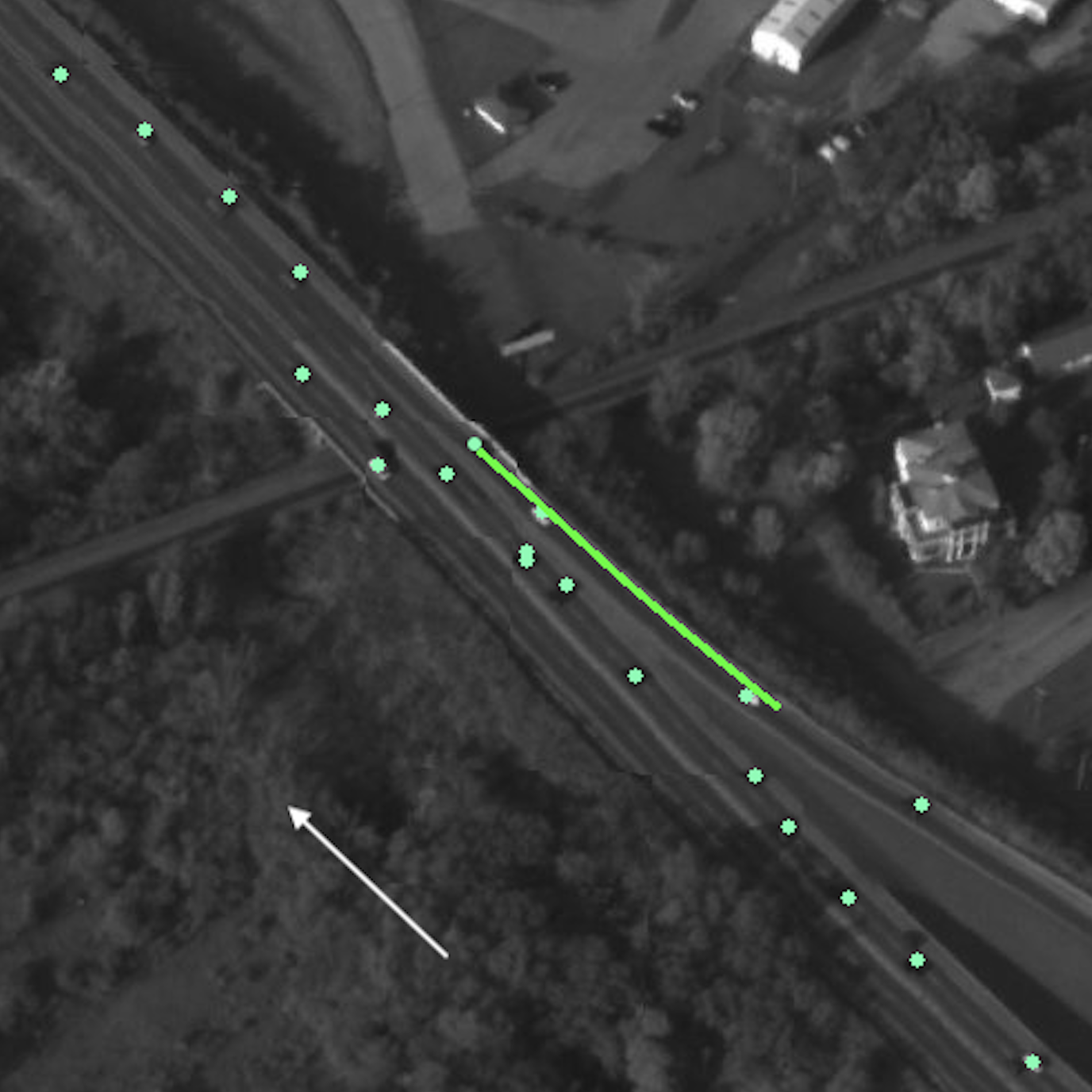
(a) tracking without attack

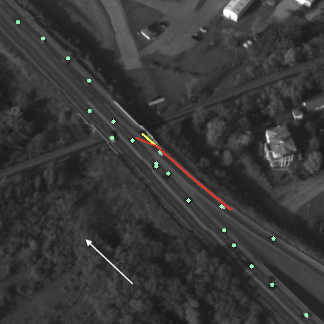
(b) tracking with attack

Figure 10: Comparison between tracking with single KF and joint KFs

In Figure 10(a), the green line represents the original track and the green dots are vehicles detected by the system. Obviously, the whole system operates normally and continuously tracks the target vehicle. However, when we attack the detection component at this time step, as shown in Figure 10(b), the current observation becomes invisible to the system. While using the original approach, the track is deviated to the nearest vehicle (see the red line). When the joint KFs are applied, since the surrounding vehicles are associated to other trackers, the primary tracker will not be associated with a wrong observation and will skip the update phase (and move along the yellow line). Thus, after the attack is stopped, the track is always correct and can finally be associated to the true target (as shown in Figure 10(b) where the yellow line overlays the green line). In the experiments, we discovered that the application of joint KFs is very effective when dealing with an attack when the vehicle traveses on a straight line, but it can be less sufficient when the attack activates while the true track is curved. This is because we adopt a constant velocity model within the dynamic model of the tracker, which is not optimal to describe the case: it makes the mean of the prediction always on a straight line and does not consider the potential direction of the movement. Therefore, when there are many detections, the data association is more likely to be wrong and lead to a larger deviation.

Table 4: The outcome of robustness and resilience verification for test scene in Figure 7 with joint-KFs and Runtime Monitor (it should be read in comparison with Table 3).

	Robustness Verification	Resilience Verification
$sol_{opt}(M,\phi)$	inf.	53.65
$\theta^{*}$	inf.	30.51
$\rho^{*}$	none	remain same

To understand how the above two techniques collectively improve the robustness and resilience, we consider the experiments described in Section 8.5, with the improvement of using joint-KFs as data association method and the attaching a runtime monitor to the tracker that are described in Section 4.

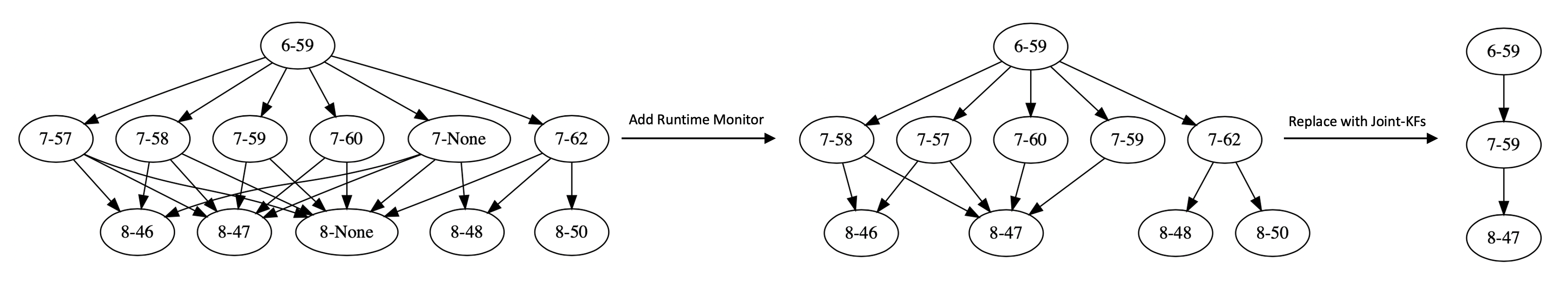
Figure 11: Improvement to WAMI tracking system by Runtime Monitor and joint-KFs (Possible adversarial tracks are reduced).

Generally speaking, after enumerating all the possible tracks, we only get the original (and true) track, with all adversarial tracks being removed. Examining Figure 11, if we attach a runtime monitor to the system, those tracks that lack observations at some steps (detection ID is None) can be detected and eliminated. Furthermore, if we replace the system’s tracking component with joint-KFs, the system can be protected from influence by incorrect observations. These two methods combined together are effective to prevent any successful attack and thereby improve the tracking robustness. As shown in Table 4, since no adversarial track exists, the attack payoff can be theoretically infinite. In practice, the payoff is usually constrained and we can introduce an oracle to judge if the very high attack payoff is valid or not. For example, too much noise added to the image will make it unrecognized by the system.

Regarding the resilience of the tracker, there is no evidence that the improvement methods have made a difference, even though all adversarial tracks (shown in Table 2) are eliminated successfully. The reason is that when the track has switched to a wrong target (by using large $dist^{max}$, which is the case we test in determining the possibility of resilience), the history information of the true target is lost. The Kalman filter is designed to estimate the state of one object with some assumptions, and resilience to a extreme noise is beyond its capacity.

We remark that, to improve the resilience, extra component(s) that processes additional information about the target vehicle is needed, for example considering different appearances of the vehicles and the context of the road network. With this kind of knowledge, the tracking system can incorporate a way to respond to the errors, and when the track is dramatically deviated, correct itself back. This will be investigated in future work. However, what can be re-emphasised from the experiments is that the robustness and the resilience are indeed different.

We have the following takeaway message to RQ4:

The runtime monitor approach can eliminate some wrong tracks, and the joint-KFs approach can reduce the risks of being influenced by wrong observations. Both of them are effective in improving the robustness, but less so for the resilience.

9 Discussion: Robustness vs. Resilience

In the discussion above, robustness and resilience can be seen as complementary concepts for the safety of a system – they express different safety aspects of the system in dealing with uncertainties. Robustness considers whether the system is tolerant, i.e., functions as usual, under the external change to the input. By contrast, resilience considers whether the system can recover from serious damages, resume part of the designed functionality, and even show signs of managing the damages.

We note here that the definition of robustness that has become generally accepted in the study of Artificial Intelligence (in particular adversarial behaviour) differs from that traditionally found in Software Engineering for critical systems where the definition relates to the systems ability to function correctly in the presence of invalid inputs (e.g. see the IEEE standard for software vocabulary [51]). Surprisingly, resilience is not defined therein, possibly due to the relative newness of the field. However, Murray et. al [52] draw together several sources to suggest that resilient software should have the capacity to withstand and recover from the failure of a critical component in a timely manner. This ties in with our definition in Subsection 6.2, but can be considered as narrower since it does not extend to attributes that may prevent component failure (as in dealing with external perturbations). To facilitate the move toward integrating ML technologies in high-integrity software engineer practices the following recommendation is made:

The definitions currently being adopted in state-of-the-art ML research, such as robustness and resilience, should be aligned to existing and accepted software engineering definitions.

In the experimental sections such as Section 8.5, examples have been provided to show the difference between robustness (in the context of ML) and resilience on the LE-SESs. In the following, we discuss a few aspects that are not covered in the LE-SESs.

9.1 End-to-End Learning based on Feedforward Network

Consider an end-to-end learning system where the entire system itself is a feedforward neural network – for example a convolutional neural network as in the NVIDIA DAVE-2 self-driving car [53]. A feedforward network is usually regarded as an instantaneous decision making mechanism, and treated as a “black-box”. These two assumptions mean that there is no temporal dimension to be considered. Therefore, we have that $l=0$ and $m=u=e=1$, for definitions in Equation (23) and Equation (25). Further, if the adversarial perturbation [9] is the only source of uncertainties to the system, we have

$$dist^{max}=dist^{1,1}(\rho,\widetilde{\rho})=\varphi^{0,1}(\widetilde{\rho})=\varphi^{l,u}(\widetilde{\rho})$$ (29)

and

$$dist^{0,e}(\rho,\widetilde{\rho})=dist^{0,1}(\rho,\widetilde{\rho})=$$ (30)

$$dist^{1,1}(\rho,\widetilde{\rho})=dist^{e,e}(\rho,\widetilde{\rho})$$

i.e., both the objective and the constraints of Equation (23) and Equation (25) are the same.

It may be justifiable that the above-mentioned equivalence of robustness and resilience is valid because, for instantaneous decision making, both properties are focused on the resistance – i.e., to resist the change and maintain the functionality of the system – and less so on the adaptability – i.e., adapt the behaviour to accommodate the change. Plainly, there is no time for recovering from the damages and showing the sign of managing the risks. Moreover, it may be that the feedforward neural network is a deterministic function, i.e., every input is assigned with a deterministic output, so there is no recovering mechanism that can be implemented.

Nevertheless, the equivalence is somewhat counter-intuitive – it is generally believed that robustness and resilience are related but not equivalent. We believe this contradiction may be from the assumptions of instantaneous decision making and black-box. If we relax the assumptions, we will find that some equations – such as $l=0$, $m=u=e=1$, and Equations (29) and (30) – do not hold any more. Actually, even for a feedforward neural network, its decision making can be seen as a sequential process, going through input layer, hidden layers, to output layer. That is, by taking a white-box analysis method, there is an internal temporal dimension. If so, the definitions in Equation (23) and Equation (25) do not equate, and capture different aspects of the feedforward network tolerating the faults, as they do for the LE-SESs. Actually, robustness is to ensure that the overall sequential process does not diverge, while resilience is to ensure that the hidden representation within a certain layer does not diverge. We remark that this robustness definition is different from that of [9]. Up to now, we are not aware of any research directly dealing with a definition of resilient neural networks. For robustness, there is some research (such as [54, 55]) suggesting that this definition implies that of [9], without providing a formal definition and evaluation method, as we have done.

Beyond feedforward neural networks, it will be an interesting topic to understand the similarity and difference of robustness and resilience, and how to improve them, for other categories of machine learning systems, such as deep reinforcement learning and recurrent neural networks, both of which have temporal dimension. We believe our definitions can be generalised to work with these systems.

9.2 Showing Sign of Recovering

For resilience, it is not required to always return to where the system was before the occurrence of the failure. Instead, it can resume part of its functionality. In this paper, for the LE-SESs, we define the status of “recovered” to be $dist^{e,e}(\rho,\widetilde{\rho})\leq\epsilon_{resilience}$, i.e., the distance of the final location of the attacked track is close to that of the original track, within a certain threshold. While the status of “recovered” can be defined, it is harder to “show the sign of recovering”, which is a subjective evaluation of the system’s recovering progress from an outside observer’s point of view. An outside observer does not necessarily have the full details of the recovering process, or the full details of the system implementation. Instead, an observer might conduct Bayesian inference or epistemic reasoning [56] by collecting evidence of recovering. Technically, a run-time monitor can be utilised to closely monitor some measurements of the recovering process; indeed, the runtime monitor we used for Kalman filter convergence (Section 4.1) can be seen as a monitor of the sign of recovering. If the Bayesian uncertainty is gradually reduced and converging, this can be considered evidence that the system is managing the failure. On the other hand, if the Bayesian uncertainty is fluctuating, we cannot claim signs of recovery, even if it might recover in the end, i.e., satisfying the condition $dist^{e,e}(\rho,\widetilde{\rho})\leq\epsilon_{resilience}$.

9.3 Resilience over Component Failure

In the paper, we consider the uncertainties from the external environment of the system, or more specifically, the adversarial attacks on the inputs to the perception unit. While this might be sufficient for robustness, which quantifies the ability to deal with erroneous input, there are other uncertainties – such as internal component failure – that may be worthy of consideration when working with resilience, because resilience may include not only the ability to deal with erroneous input but also the ability to cope with, and recover from, component failure, as suggested in e.g., Murray et. al [52] in software engineering.

In LE-SESs, the component failure may include the failure of a perceptional unit or the failure of a Bayes filter. The failures of Bayes filter may include e.g., missing or perturbed values in the matrices $\mathbf{F}$, $\mathbf{H}$, $\mathbf{Q}$, and $\mathbf{R}$. The failures of the perceptional unit may include e.g., the failure of interactions between neural networks, the internal component failure of a neural network (e.g., some neuron does not function correctly), etc. The study of component failures, and their impact to resilience, will be considered in our future work.

10 Related Work

Below, we review research relevant to the verification of robustness and resilience for learning-enabled systems.

10.1 Safety Analysis of Learning Enabled Systems

ML techniques have been confirmed to have potential safety risks [57]. Currently, most safety verification and validation work focuses on the ML components, including formal verification [12, 13, 14, 15, 16, 17, 18, 19, 20, 21] and coverage-guided testing [22, 23, 24, 25, 26, 27, 28, 29]. Please refer to [30] for a recent survey on the progress of this area.

Research is sparse at the system level, and there is none (apparent) on state estimation systems. In [58], a compositional framework is developed for the falsification of temporal logic properties of cyber-physical systems with ML components. Their approaches are applied to an Automatic Emergency Braking System. A simulation based approach [59] is suggested to verify the barrier certificates – representing safety invariants – of autonomous driving systems with an SMT solver. In both papers, the interaction – or synchronisation – between ML and other components is through a shared value, which is drastically different from the neural network enabled state estimation, where the synchronisation is closer to the message-passing regime. Moreover, the erroneous behaviours and the specifications of this paper are different from those of [58, 59]. These differences suggest that the existing approaches cannot be extended to work with our problem.

In addition, in [60], a system with a sigmoid-based neural network as the controller is transformed into a hybrid system, on which the verification can be solved with existing tools. This approach may not generalise to general neural networks since it heavily relies on the fact that the sigmoid is the solution to a quadratic differential equation. In [61], a gray-box testing approach is proposed for systems with learning-based controllers, where a gradient based method is taken to search the input space. This approach is heuristic, and based on the assumption that the system is differentiable. The LE-SESs cannot be verified with these approaches.

Moreover, there is some early research on the robustness of KF by false information injection[62, 63], where the false information is modelled as Gaussian noise, differing from our consideration of adversarial attacks.

10.2 Robustness and Resilience

The endeavours of defining the two views – robustness and resilience – of a system’s predictable operational outcome are widely abound from various perspectives. For example, from the automation study [64, 65], robustness is strongly attached with a pre-oriented purpose with designated value and judgment from which some criteria, such as “correctness” and “validity”, are imposed for checking against a system or a component. This view, with others focusing on the safety and risk aversion as reviewed in Section 10.1, casts some light on the degree of sticking with pre-set criteria with toleration to an aggregated deviation. In fact, discussion has rarely been extended to the flip side of this notion, which is resilience.

Resilience captures the other stream of features, especially from social science system, such as implicitly embedded openness, multi-dimensionality, adaptive accommodation, and diversity in value and evolution. These under-discussed features deserve more attention such that they be integrated into the effort in understanding resilience in AI. Indeed, before the terms formally appeared in many representative multidisciplinary studies such as system and environmental research[46], there were works on methodological discussions about robustness and resilience. In [66], the author discusses the robustness and resilience in a social system through the investigation of human societies relevant to explicating human behavior. It is further discovered that self-monitoring of the state of a system – coincidence with our enhancement techniques through runtime monitoring – is important both as part of robustness and resilience. In [67], four properties of a system – risk, vulnerability, robustness, and resilience – are compared from decision theoretical perspective; it argues that robustness can be seen as an antonym to (static) vulnerability, and resilience equal to (dynamic) vulnerability as the adverse events linked to threats/hazards to which a system is exposed to are known. This statement is close to our definitions. Beyond these methodological discussions, in this paper, we exemplify the distinction between robustness and resilience in a learning-enabled autonomous system and formally verify these two properties.

Whilst these wider considerations of robustness and resilience are useful, we restate our earlier insight that there are differences between the definitions in ML applications and that of the wider software engineering community, including the IEEE standards, that should be resolved.

11 Conclusion

This paper provides a formal verification guided approach for the design of learning-enabled state estimation systems. Empirically our initial design of the state estimation system performs well for its tracking task, its weaknesses in robustness and resilience are exploited by our formal verification approach. This leads to our enhanced design of the system, on which the robustness is improved.

The research conducted in this paper is motivation for a number of follow-up research activities. First of all, while our definitions for robustness and resilience are general for LE-SESs, an in-depth study is required to understand if, and how, to generalise them to a broader set of learning-enabled autonomous systems. Second, runtime verification techniques are worthy of further consideration. The formal verification technique is shown to be NP-complete for robustness. Our verification algorithm works well for the WAMI tracking system since we conduct off-line analysis. A lightweight runtime verification technique will be especially helpful if we intend to work with large-scale, networked systems with hundreds or thousands of components. Third, more approaches for the improvement of robustness and resilience are needed. We have investigated two approaches: (1) the utility of joining collaborative components and (2) the utility of a runtime monitor. The exploration of other approaches, and comparison of their relative effectiveness, will be an interesting topic.

References

- [1] Wei Huang, Yifan Zhou, Gaojie Jin, Youcheng Sun, Alec Banks, Jie Meng, James Sharp, Simon Maskell, and Xiaowei Huang. Formal verification of robustness and resilience of learning-enabled state estimation systems for robotics. arXiv preprint arXiv:2010.08311, 2020.
- [2] Youcheng Sun, Yifan Zhou, Simon Maskell, James Sharp, and Xiaowei Huang. Reliability validation of learning enabled vehicle tracking. In ICRA, 2020.
- [3] Wei Huang, Yifan Zhou, Youcheng Sun, James Sharp, Simon Maskell, and Xiaowei Huang. Practical verification of neural network enabled state estimation system for robotics. In 2020 IEEE/RSJ International Conference on Intelligent Robots and Systems (IROS), pages 7336–7343, 2020.
- [4] Joseph Sifakis. Autonomous systems - an architectural characterization. CoRR, abs/1811.10277, 2018.
- [5] Georgios Papadopoulos, Maurice F Fallon, John J Leonard, and Nicholas M Patrikalakis. Cooperative localization of marine vehicles using nonlinear state estimation. In International Conference on Intelligent Robots and Systems, pages 4874–4879. IEEE, 2010.
- [6] Neil Gordon, David Salmond, and Craig Ewing. Bayesian state estimation for tracking and guidance using the bootstrap filter. Journal of Guidance, Control, and Dynamics, 18(6):1434–1443, 1995.
- [7] Y. Zhou and S. Maskell. Detecting and tracking small moving objects in wide area motion imagery (wami) using convolutional neural networks (cnns). In 2019 22th International Conference on Information Fusion (FUSION), pages 1–8, July 2019.
- [8] Wei He and Yiting Dong. Adaptive fuzzy neural network control for a constrained robot using impedance learning. IEEE transactions on neural networks and learning systems, 2017.
- [9] Christian Szegedy, Wojciech Zaremba, Ilya Sutskever, Joan Bruna, Dumitru Erhan, Ian Goodfellow, and Rob Fergus. Intriguing properties of neural networks. In ICLR2014, 2014.
- [10] N. Papernot, P. McDaniel, X. Wu, S. Jha, and A. Swami. Distillation as a defense to adversarial perturbations against deep neural networks. In 2016 IEEE Symposium on Security and Privacy (SP), pages 582–597, May 2016.
- [11] Nicholas Carlini and David Wagner. Towards evaluating the robustness of neural networks. In Security and Privacy (SP), IEEE Symposium on, pages 39–57, 2017.
- [12] Xiaowei Huang, Marta Kwiatkowska, Sen Wang, and Min Wu. Safety verification of deep neural networks. In CAV2017, 2017.
- [13] Guy Katz, Clark Barrett, David L Dill, Kyle Julian, and Mykel J Kochenderfer. Reluplex: An efficient SMT solver for verifying deep neural networks. In International Conference on Computer Aided Verification, pages 97–117. Springer, 2017.
- [14] Weiming Xiang, Hoang-Dung Tran, and Taylor T Johnson. Output reachable set estimation and verification for multi-layer neural networks. IEEE Transactions on Neural Networks and Learning Systems, 29:5777–5783, 2018.
- [15] T. Gehr, M. Mirman, D. Drachsler-Cohen, P. Tsankov, S. Chaudhuri, and M. Vechev. Ai2: Safety and robustness certification of neural networks with abstract interpretation. In 2018 IEEE Symposium on Security and Privacy (S&P2018), pages 948–963, 2018.
- [16] Alessio Lomuscio and Lalit Maganti. An approach to reachability analysis for feed-forward ReLU neural networks. arXiv preprint arXiv:1706.07351, 2017.
- [17] Matthew Wicker, Xiaowei Huang, and Marta Kwiatkowska. Feature-guided black-box safety testing of deep neural networks. In TACAS2018, pages 408–426, 2018.
- [18] Wenjie Ruan, Xiaowei Huang, and Marta Kwiatkowska. Reachability analysis of deep neural networks with provable guarantees. In IJCAI, pages 2651–2659, 2018.
- [19] Min Wu, Matthew Wicker, Wenjie Ruan, Xiaowei Huang, and Marta Kwiatkowska. A game-based approximate verification of deep neural networks with provable guarantees. Theoretical Computer Science, 2019.
- [20] Wenjie Ruan, Min Wu, Youcheng Sun, Xiaowei Huang, Daniel Kroening, and Marta Kwiatkowska. Global robustness evaluation of deep neural networks with provable guarantees for hamming distance. In IJCAI2019, 2019.
- [21] Jianlin Li, Jiangchao Liu, Pengfei Yang, Liqian Chen, and Xiaowei Huang. Analyzing deep neural networks with symbolic propagation: Towards higher precision and faster verification. Submitted, 2018.
- [22] Youcheng Sun, Min Wu, Wenjie Ruan, Xiaowei Huang, Marta Kwiatkowska, and Daniel Kroening. Concolic testing for deep neural networks. In ASE, 2018.
- [23] Kexin Pei, Yinzhi Cao, Junfeng Yang, and Suman Jana. DeepXplore: Automated whitebox testing of deep learning systems. In Proceedings of the 26th Symposium on Operating Systems Principles, pages 1–18. ACM, 2017.
- [24] Youcheng Sun, Xiaowei Huang, Daniel Kroening, James Sharp, Matthew Hill, and Rob Ashmore. Structural test coverage criteria for deep neural networks. ACM Trans. Embed. Comput. Syst., 18(5s), October 2019.
- [25] Lei Ma, Felix Juefei-Xu, Jiyuan Sun, Chunyang Chen, Ting Su, Fuyuan Zhang, Minhui Xue, Bo Li, Li Li, Yang Liu, Jianjun Zhao, and Yadong Wang. DeepGauge: Comprehensive and multi-granularity testing criteria for gauging the robustness of deep learning systems. In Automated Software Engineering (ASE), 33rd IEEE/ACM International Conference on, 2018.
- [26] Youcheng Sun, Xiaowei Huang, Daniel Kroening, James Sharp, Matthew Hill, and Rob Ashmore. DeepConcolic: testing and debugging deep neural networks. In 41st International Conference on Software Engineering: Companion Proceedings (ICSE-Companion), pages 111–114. IEEE, 2019.
- [27] Wei Huang, Youcheng Sun, James Sharp, and Xiaowei Huang. Test metrics for recurrent neural networks. arXiv preprint arXiv:1911.01952, 2019.
- [28] Wei Huang, Youcheng Sun, Xiaowei Huang, and James Sharp. testRNN: Coverage-guided testing on recurrent neural networks. arXiv preprint arXiv:1906.08557, 2019.
- [29] Yannic Noller, Corina S Păsăreanu, Marcel Böhme, Youcheng Sun, Hoang Lam Nguyen, and Lars Grunske. HyDiff: Hybrid differential software analysis. In Proceedings of the 42nd International Conference on Software Engineering, ICSE, 2020.
- [30] Xiaowei Huang, Daniel Kroening, Wenjie Ruan, James Sharp, Youcheng Sun, Emese Thamo, Min Wu, and Xinping Yi. A survey of safety and trustworthiness of deep neural networks. arXiv preprint arXiv:1812.08342, 2018.
- [31] Y. Zhou and S. Maskell. Detecting and tracking small moving objects in wide area motion imagery (wami) using convolutional neural networks (cnns). In 2019 22th International Conference on Information Fusion (FUSION), pages 1–8, Ottawa, ON, Canada, July 2019.
- [32] AFRL. Wright-patterson air force base (wpafb) dataset. https://www.sdms.afrl.af.mil/index.php?collection=wpafb2009, 2009.
- [33] Lars Wilko Sommer, Michael Teutsch, Tobias Schuchert, and Jürgen Beyerer. A survey on moving object detection for wide area motion imagery. In IEEE Winter Conference on Applications of Computer Vision, WACV, pages 1–9, 2016.
- [34] Rodney LaLonde, Dong Zhang, and Mubarak Shah. Clusternet: Detecting small objects in large scenes by exploiting spatio-temporal information. In CVPR, pages 4003–4012, 2018.
- [35] David G. Lowe. Distinctive image features from scale-invariant keypoints. Int. J. Comput. Vision, 60(2):91–110, November 2004.
- [36] Herbert Bay, Tinne Tuytelaars, and Luc Van Gool. Surf: Speeded up robust features. In Aleš Leonardis, Horst Bischof, and Axel Pinz, editors, Computer Vision – ECCV, pages 404–417, Berlin, Heidelberg, 2006. Springer Berlin Heidelberg.
- [37] E. Rublee, V. Rabaud, K. Konolige, and G. Bradski. Orb: An efficient alternative to sift or surf. In International Conference on Computer Vision, pages 2564–2571, Nov 2011.
- [38] Martin A. Fischler and Robert C. Bolles. Random sample consensus: A paradigm for model fitting with applications to image analysis and automated cartography. Commun. ACM, 24(6):381–395, June 1981.
- [39] R. E. Kalman. A new approach to linear filtering and prediction problems. J. Basic Eng., 82(1):35–45, 1960.
- [40] Seyed-Mohsen Moosavi-Dezfooli, Alhussein Fawzi, and Pascal Frossard. Deepfool: a simple and accurate method to fool deep neural networks. In Proceedings of the IEEE Conference on Computer Vision and Pattern Recognition, pages 2574–2582, 2016.
- [41] Edmund M Clarke Jr, Orna Grumberg, Daniel Kroening, Doron Peled, and Helmut Veith. Model checking. The MIT Press, 2018.
- [42] John Ruscio. A probability-based measure of effect size: Robustness to base rates and other factors. Psychological methods, 13(1):19, 2008.
- [43] Y Vander Heyden, A Nijhuis, J Smeyers-Verbeke, BGM Vandeginste, and DL Massart. Guidance for robustness/ruggedness tests in method validation. Journal of pharmaceutical and biomedical analysis, 24(5-6):723–753, 2001.
- [44] Didier Gonze, José Halloy, and Pierre Gaspard. Biochemical clocks and molecular noise: Theoretical study of robustness factors. The Journal of chemical physics, 116(24):10997–11010, 2002.
- [45] Emmy E Werner. Risk, resilience, and recovery: Perspectives from the kauai longitudinal study. Development and psychopathology, 5(4):503–515, 1993.
- [46] Ann Dale, Chris Ling, and Lenore Newman. Community vitality: The role of community-level resilience adaptation and innovation in sustainable development. Sustainability, 2(1):215–231, 2010.
- [47] Carl Folke, Steve Carpenter, Brian Walker, Marten Scheffer, Thomas Elmqvist, Lance Gunderson, and Crawford Stanley Holling. Regime shifts, resilience, and biodiversity in ecosystem management. Annu. Rev. Ecol. Evol. Syst., 35:557–581, 2004.
- [48] Keri Black and Marie Lobo. A conceptual review of family resilience factors. Journal of family nursing, 14(1):33–55, 2008.
- [49] Cale Palmer. A theory of risk and resilience factors in military families. Military Psychology, 20(3):205–217, 2008.
- [50] Bruce W Smith, Jeanne Dalen, Kathryn Wiggins, Erin Tooley, Paulette Christopher, and Jennifer Bernard. The brief resilience scale: assessing the ability to bounce back. International journal of behavioral medicine, 15(3):194–200, 2008.
- [51] Iso/iec/ieee international standard - systems and software engineering–vocabulary. ISO/IEC/IEEE 24765:2017(E), pages 1–541, 2017.
- [52] Acklyn Murray, Marlon Mejias, and Peter Keiller. Resilience methods within the software development cycle. International Conference on Software Engineering, Research and Practice, SERP’17, 2017.
- [53] Mariusz Bojarski, Davide Del Testa, Daniel Dworakowski, Bernhard Firner, Beat Flepp, Prasoon Goyal, Lawrence D. Jackel, Mathew Monfort, Urs Muller, Jiakai Zhang, Xin Zhang, Jake Zhao, and Karol Zieba. End to end learning for self-driving cars. CoRR, abs/1604.07316, 2016.
- [54] Jan Hendrik Metzen, Tim Genewein, Volker Fischer, and Bastian Bischoff. On Detecting Adversarial Perturbations. In ICLR2017, 2017.
- [55] Francesco Crecchi, Davide Bacciu, and Battista Biggio. Detecting Adversarial Examples through Nonlinear Dimensionality Reduction. In ESANN2019, 2019.
- [56] CJoseph Y. Halpern. Reasoning about Uncertainty. The MIT Press, 2017.
- [57] Ian J Goodfellow, Jonathon Shlens, and Christian Szegedy. Explaining and harnessing adversarial examples (2014). arXiv preprint arXiv:1412.6572.
- [58] Tommaso Dreossi, Alexandre Donzé, and Sanjit A Seshia. Compositional falsification of cyber-physical systems with machine learning components. Journal of Automated Reasoning, 63(4):1031–1053, 2019.
- [59] Cumhur Erkan Tuncali, James Kapinski, Hisahiro Ito, and Jyotirmoy V Deshmukh. Reasoning about safety of learning-enabled components in autonomous cyber-physical systems. arXiv preprint arXiv:1804.03973, 2018.
- [60] Radoslav Ivanov, James Weimer, Rajeev Alur, George J. Pappas, and Insup Lee. Verisig: Verifying safety properties of hybrid systems with neural network controllers. In Proceedings of the 22nd ACM International Conference on Hybrid Systems: Computation and Control, HSCC ’19, page 169–178, New York, NY, USA, 2019. Association for Computing Machinery.
- [61] Shakiba Yaghoubi and Georgios Fainekos. Gray-box adversarial testing for control systems with machine learning components. In Proceedings of the 22nd ACM International Conference on Hybrid Systems: Computation and Control, HSCC ’19, page 179–184, New York, NY, USA, 2019. Association for Computing Machinery.
- [62] Ruixin Niu and Lauren Huie. System state estimation in the presence of false information injection. In Statistical Signal Processing Workshop (SSP), pages 385–388. IEEE, 2012.
- [63] Qingyu Yang, Liguo Chang, and Wei Yu. On false data injection attacks against kalman filtering in power system dynamic state estimation. Security and Communication Networks, 9(9):833–849, 2016.
- [64] Craig G Rieger. Resilient control systems practical metrics basis for defining mission impact. In 2014 7th International Symposium on Resilient Control Systems (ISRCS), pages 1–10. IEEE, 2014.
- [65] Royce Francis and Behailu Bekera. A metric and frameworks for resilience analysis of engineered and infrastructure systems. Reliability Engineering & System Safety, 121:90–103, 2014.
- [66] Dwight Read. Some observations on resilience and robustness in human systems. Cybernetics and Systems: An International Journal, 36(8):773–802, 2005.
- [67] Roland W Scholz, Yann B Blumer, and Fridolin S Brand. Risk, vulnerability, robustness, and resilience from a decision-theoretic perspective. Journal of Risk Research, 15(3):313–330, 2012.