Training Data Generating Networks: Shape Reconstruction via Bi-level Optimization
Abstract
We propose a novel 3d shape representation for 3d shape reconstruction from a single image. Rather than predicting a shape directly, we train a network to generate a training set which will be fed into another learning algorithm to define the shape. The nested optimization problem can be modeled by bi-level optimization. Specifically, the algorithms for bi-level optimization are also being used in meta learning approaches for few-shot learning. Our framework establishes a link between 3D shape analysis and few-shot learning. We combine training data generating networks with bi-level optimization algorithms to obtain a complete framework for which all components can be jointly trained. We improve upon recent work on standard benchmarks for 3d shape reconstruction.
1 Introduction
Neural networks have shown promising results for shape reconstruction (Wang et al., 2018; Groueix et al., 2018; Mescheder et al., 2019; Genova et al., 2019). Different from the image domain, there is no universally agreed upon way to represent 3d shapes. There exist many explicit and implicit representations. Explicit representations include point clouds (Qi et al., 2017a; b; Lin et al., 2017), grids (Wu et al., 2015; Choy et al., 2016; Riegler et al., 2017; Wang et al., 2017; Tatarchenko et al., 2017), and meshes (Wang et al., 2018; Hanocka et al., 2019). Implicit representations (Mescheder et al., 2019; Michalkiewicz et al., 2019; Park et al., 2019) define shapes as iso-surfaces of functions. Both types of representations are important as they have different advantages.
In this work, we set out to investigate how meta-learning can be used to learn shape representations. To employ meta-learning, we need to split the learning framework into two (or more) coupled learning problems. There are multiple design choices for exploring this idea. One related solution is to use a hypernetwork as the first learning algorithm that produces the weights for a second network. This approach (Littwin & Wolf, 2019), is very inspiring, but the results can still be improved by our work. The value of our work are not mainly the state-of-the-art results, but the new framework that enables the flow of new ideas, techniques, and methods developed in the context of few-shot learning and meta-optimization to be applied to shape reconstruction.
In order to derive our proposed solution, we draw inspiration from few-shot learning. The formulation of few-shot learning we use here is similar to Lee et al. (2019); Bertinetto et al. (2019), but also other formulations of few shot learning exist, e.g., MAML (Finn et al., 2017). In few-shot learning for image classification, the learning problem is split into multiple tasks (See Fig. 1). For each task, the learning framework has to learn a decision boundary to distinguish between a smaller set of classes. In order to do so, a first network is used to embed images into a high-dimensional feature space. A second learner (often called base learner in the literature of meta learning approaches for few-shot learning) is then used to learn decision boundaries in this high-dimensional feature space. A key point is that each task has separate decision boundaries. In order to build a bridge from few-shot learning to shape representations, we identify each shape as a separate task. For each task, there are two classes to distinguish: inside and outside. The link might seem a bit unintuitive at first, because in the image classification case, each task is defined by multiple images already divided into multiple classes. However, in our case, a task is only associated with a single image. We therefore introduce an additional component, a training data generating network, to build the bridge to few-shot learning (See Fig. 2). This training data generating network takes a single image as input and outputs multiple 3D points with an inside and outside label. These points define the training dataset for one task (shape). We adopt this data set format to describe a task, because points are a natural shape representation. Similar to the image classification setting, we also employ an embedding network that maps the original training dataset (a set of 3D points) to another space where it is easier to find a decision boundary (a distorted 3D space). In contrast to the image classification setting, the input and output spaces of the embedding network have a lot fewer dimensions, i.e. only three dimensions. Next, we have to tackle the base learner that takes a set of points in embedding space as input. Here, we can draw from multiple options. In particular, we experimented with kernel SVMs and kernel ridge regression. As both give similar results (In meta learning (Lee et al., 2019) we can also find the same conclusion), we opted for ridge regression in our solution due to the much faster processing time. The goal of ridge regression is to learn a decision boundary (shape surface) in 3D space describing the shape.
Our intermediate shape representation is a set of points, but these points cannot be chosen arbitrarily. The set of points are specifically generated so that the second learning algorithm can process them to find a decision boundary. The second learning algorithm functions similar to other implicit shape representations discussed above. The result of the second learning algorithm (SVM or ridge regression) can be queried as an implicit function. Still the second learning algorithm cannot be replaced by other existing networks employed in previous work. Therefore, among existing works, only our representation can directly use few-shot learning. It does not make sense to train our representation without a few-shot learning framework and no other representation can be directly trained with a few-shot learning framework. Therefore, all components in our framework are intrinsically linked and were designed together.
Contributions.
-
•
We propose a new type of shape representation, where we train a network to output a training set (a set of labeled points) for another machine learning algorithm (Kernel Ridge Regression or Kernel-SVM).
-
•
We found an elegant way to map the problem of shape reconstruction from a single image to the problem of few-shot classification by introducing a network to generate training data. We combined training data generating networks with two meta learning approaches (R2D2 (Bertinetto et al., 2019) and MetaOptNet (Lee et al., 2019)) in our framework. Our work enables the application of ideas and techniques developed in the few-shot learning literature to the problem of shape reconstruction.
-
•
We validate our model using the problem of 3d shape reconstruction from a single image and improve upon the state of the art.
2 Related work
Neural implicit shape representations.
We can identify two major categories of shape representations: explicit representations, where a shape can be explicitly defined; and implicit representations, where a shape can be defined as iso-surface of a function (signed distance function or indicator function). In the past decade, we have seen great success with neural network based explicit shape representations: voxel representations (Wu et al., 2015; Choy et al., 2016; Riegler et al., 2017; Wang et al., 2017; Tatarchenko et al., 2017), point representations (Qi et al., 2017a; b; Fan et al., 2017; Lin et al., 2017), and mesh representations (Wang et al., 2018; Hanocka et al., 2019)). On the other hand, modeling implicit representations with neural networks has been a current trend, where usually a signed distance function or indicator function is parameterized by a neural network (Mescheder et al., 2019; Chen & Zhang, 2019; Michalkiewicz et al., 2019; Park et al., 2019). More recent works learn a network that outputs intermediate parameters, e.g. CvxNet (Deng et al., 2019) and BSP-Net (Chen et al., 2019) learns to output half-spaces. We propose a novel type of shape representation, where the model outputs a training set of labeled points.
Few-shot learning.
There are two common meta learning approaches for few-shot learning: metric-based (Koch et al., 2015; Vinyals et al., 2016; Snell et al., 2017), which aims to learn a metric for each task; optimization-based (Ravi & Larochelle, 2017; Finn et al., 2017; Nichol et al., 2018), which is designed to learn with a few training samples by adjusting optimization algorithms. These approaches commonly have two parts, an embedding model for mapping an input to an embedding space, and a base learner for prediction. Qiao et al. (2018); Gidaris & Komodakis (2018) train a hypernetwork (Ha et al., 2016) to output weights of another network (base learner). R2D2 (Bertinetto et al., 2019) showed that using a light-weight and differentiable base learner (e.g. ridge regression) leads to better results. To further develop the idea, MetaOptNet (Lee et al., 2019) used multi-class support vector machines (Crammer & Singer, 2001) as base learner and incorporated differentiable optimization (Amos & Kolter, 2017; Gould et al., 2016) into the framework. Lee et al. (2019) also shows it can outperform hypernetwork-based methods. In our work, we propose a shape representation that is compatible with a few-shot classification framework so that we can utilize existing meta learning approaches. Specifically, we will use ridge regression and SVM as the base learner. The most relevant method to ours is Littwin & Wolf (2019) which adapts hypernetworks. However, as we discussed above, differentiable optimization methods (Bertinetto et al., 2019; Lee et al., 2019) are generally better than hypernetworks. Besides that, meta learning has been applied to other fields in shape analysis, e.g., both Sitzmann et al. (2020) and Tancik et al. (2021) propose to use MAML-like algorithms (Finn et al., 2017) to learn a weight initialization.
3 Method
The framework is shown in Fig. 2. The network is mainly composed of 3 sub-networks. The Feature Network maps an input image to feature space. The resulting feature vector is then decoded by the Point Generation Network to a labeled point set . The point set will be used as training data in our base learner later. After that the Embedding Network projects the point set into embedding space. The projected points and the labels are taken as the input of a binary classifer (ridge regression or SVM) parameterized by . Finally, the framework is able to output the inside/outside label of a query point by projecting it into the embedding space and feeding it to the binary classifier.
In the following subsections, we describe our method in more detail. First, we introduce the background of meta learning approaches for few-show learning (Sec. 3.1) and establish a link between single image 3D reconstruction and few-shot learning (Sec. 3.2). We propose a problem formulation inspired by few-shot learning (Sec. 3.3) and propose a solution in the following subsections. Specifically, we apply recently developed differentiable optimization.
3.1 Background
Supervised learning.
Given training set , supervised learning learns a predictor which is able to predict the labels of test set (assuming both and are sampled from the same distribution).
Few-shot learning.
In few-shot learning, the size of the training set is typically small. The common learning algorithms on a single task usually cause problems like overfitting. However, we are given a collection of tasks, the meta-training set , on which we train a meta-learner which produces a predictor on every task and generalizes well on the meta-testing .
Consider a -class classification task, each training set consists of labelled examples for each of classes. The meta-training task is often referred to as -shot--way. Refer to Figure 1 for an example visualization of 2-shot-3-way few-shot image classification.
Meta learning approaches for few-shot learning often involve an embedding network, and a base learner (learning algorithm). The embedding network maps training samples to an embedding space. We explain in later subsections how the 3d reconstruction is connected to meta learning in these two aspects.
3.2 Single image 3D reconstruction
A watertight shape can be represented by an indicator (or occupancy) function . We define if is inside the object, otherwise. We can sample a set of points in and evaluate the indicator , then we have the labeled point set where . The number needs to be large enough to approximate the shape. In this way, we rewrite the target ground-truth as a point set. This strategy is also used by Mescheder et al. (2019) and Deng et al. (2019). Also see Figure 1 for an illustration.
The goal of single image 3D reconstruction is to convert an input image to the indicator function .
Previous work either directly learns (Mescheder et al., 2019))or trains a network to predict an intermediate parametric representation (e.g. collection of convex primitives (Deng et al., 2019), half-spaces (Chen et al., 2019)). Different from any existing methods, our shape representation is to generate training data for a few-shot classification problem. In order to make the connection clear, we denote the ground-truth as .
The training data of single image 3D reconstruction are a collection of images and their corresponding shapes which we denote as . The goal is to learn a network which takes as input an image and outputs a functional (predictor) which works on .
We summarize the notation and the mapping of few-shot classification to 3D shape reconstruction in Table 1. Using the proposed mapping, we need to find a data generating network (Fig. 2 left) to convert the input to a set of labeled points (usually is far smaller than ). Then the can be rewritten as . It can be seen that, this formulation has a high resemblance to few-shot learning. Also see Figure 1 for a visualization. As a result, we can leverage techniques from the literature of few-shot learning to jointly train the data generation and the classification components.
| Few-shot classification | 3D shape reconstruction | |
| - | input images | |
| - | ||
| - | ||
| images | points | |
| categories | inside/outside labels | |
| predictor | classifier | surface boundary |
3.3 Formulation
Similar to few-shot learning, the problem can be written as a bi-level optimization. The inner optimization is to train the predictor to estimate the inside/outside label of a point,
| (1) |
where is a loss function such as cross entropy. While in few-shot learning is provided or sampled, here is generated by a network , . To reconstruct the shape , the predictor should work as an approximation of the indicator and is expected to minimize the term,
| (2) |
This process is done by a base learner (machine learning algorithm) in some meta learning methods (Bertinetto et al., 2019; Lee et al., 2019).
The final objective across all shapes (tasks) is
| (3) | ||||
| s.t. |
which is exactly the same as for meta learning algorithms if we remove the constraint .
Point Embedding.
In meta learning approaches for few-shot classification, an embedding network is used to map the training samples to an embedding space, , where is the embedding vector of the input . We also migrate the idea to 3d shape representations, , where the embedding network is also conditioned on the task input .
In later sections, we use and to denote the embeddings of point and , respectively. In addition to the objective Eq equation 3, we add a regularizer,
| (4) |
where is the weight for the regularizer. There are multiple solutions for the Embedding Network, thus we want to use the regularizer to shrink potential solutions, which is to find a similar embedding space to the original one. The is set to in all experiments if not specified.
3.4 Differentiable learner
The Eq. equation 1 is the inner loop of the final objective Eq. equation 3. Recent meta learning approaches use differentiable learners, e.g., R2D2 (Bertinetto et al., 2019) uses Ridge Regression and MetaOptNet (Lee et al., 2019) uses Support Vector Machines (SVM). We describe both cases here. Different than the learner in R2D2 and MetaOptNet, we use kernelized algorithms.
Ridge Regression.
Given a training set , The kernel ridge regression (Murphy, 2012) is formulated as follows,
| (5) |
where is the data kernel matrix in which each entry is the Gaussian kernel . The solution is given by an analytic form . By using automatic differentiation of existing deep learning libraries, we can differentiate through with respect to each in . We obtain the prediction for a query point via
| (6) |
SVM.
We use the dual form of kernel SVM,
| (7) | ||||||
| subject to |
where is the Gaussian kernel. .
The discriminant function becomes,
| (8) |
Using recent advances in differentiable optimization by Amos & Kolter (2017), the discriminant function is differentiable with respect to each in .
While the definitions of both learners are given here, we only show results of ridge regression in our main paper. Additional results of SVM are provided in the supplementary material. In traditional machine learning, SVM is better than ridge regression in many aspects. However, we do not find SVM shows significant improvement over ridge regression in our experiments. The conclusion is also consistent with Lee et al. (2019).
3.5 Indicator approximation
We clip the outputs of the ridge regression to the range as an approximation of the indicator . For the SVM, the predictor outputs a positive value if is inside the shape otherwise a negative value. So we apply a sigmoid function to convert it to the range , , where is a learned scale. Then Eq. equation 2 is written as follows:
| (9) |
where the minimum squared error (MSE) loss is also used in CvxNet (Deng et al., 2019).
4 Implementation
| Categ. | IoU | Chamfer | F-Score | |||||||||||||||||||
|---|---|---|---|---|---|---|---|---|---|---|---|---|---|---|---|---|---|---|---|---|---|---|
| Ours | P2M | ON | ON† | SIF | CN | HN† | Ours | P2M | AN | ON | ON† | SIF | CN | HN† | Ours | AN | ON | ON† | SIF | CN | HN† | |
| plane | 0.633 | 0.420 | 0.571 | 0.603 | 0.530 | 0.598 | 0.608 | 0.121 | 0.187 | 0.104 | 0.147 | 0.144 | 0.167 | 0.093 | 0.127 | 71.15 | 67.24 | 62.87 | 67.25 | 52.81 | 68.16 | 68.56 |
| bench | 0.524 | 0.323 | 0.485 | 0.486 | 0.333 | 0.461 | 0.501 | 0.132 | 0.201 | 0.138 | 0.155 | 0.148 | 0.261 | 0.133 | 0.146 | 69.44 | 54.50 | 56.91 | 64.80 | 37.31 | 54.64 | 65.43 |
| cabinet | 0.732 | 0.664 | 0.733 | 0.733 | 0.648 | 0.709 | 0.734 | 0.141 | 0.196 | 0.175 | 0.167 | 0.142 | 0.233 | 0.160 | 0.145 | 65.33 | 46.43 | 61.79 | 62.78 | 31.68 | 46.09 | 63.15 |
| car | 0.748 | 0.552 | 0.737 | 0.738 | 0.657 | 0.675 | 0.732 | 0.121 | 0.180 | 0.141 | 0.159 | 0.125 | 0.161 | 0.103 | 0.131 | 65.48 | 51.51 | 56.91 | 63.68 | 37.66 | 47.33 | 61.46 |
| chair | 0.532 | 0.396 | 0.501 | 0.515 | 0.389 | 0.491 | 0.517 | 0.205 | 0.265 | 0.209 | 0.228 | 0.217 | 0.380 | 0.337 | 0.230 | 48.83 | 38.89 | 42.41 | 46.38 | 26.90 | 38.49 | 45.56 |
| display | 0.553 | 0.490 | 0.471 | 0.540 | 0.491 | 0.576 | 0.542 | 0.215 | 0.239 | 0.198 | 0.278 | 0.213 | 0.401 | 0.223 | 0.217 | 46.96 | 42.79 | 38.96 | 44.55 | 27.22 | 40.69 | 44.42 |
| lamp | 0.383 | 0.323 | 0.371 | 0.395 | 0.260 | 0.311 | 0.389 | 0.391 | 0.308 | 0.305 | 0.479 | 0.404 | 1.096 | 0.795 | 0.441 | 42.99 | 33.04 | 38.35 | 43.41 | 20.59 | 31.41 | 41.81 |
| speaker | 0.658 | 0.599 | 0.647 | 0.651 | 0.577 | 0.620 | 0.661 | 0.247 | 0.285 | 0.245 | 0.300 | 0.261 | 0.554 | 0.462 | 0.261 | 46.86 | 35.75 | 42.48 | 44.05 | 22.42 | 29.45 | 45.33 |
| rifle | 0.540 | 0.402 | 0.474 | 0.496 | 0.463 | 0.515 | 0.508 | 0.111 | 0.164 | 0.115 | 0.141 | 0.129 | 0.193 | 0.106 | 0.120 | 69.40 | 64.22 | 56.52 | 64.34 | 53.20 | 63.74 | 65.92 |
| sofa | 0.707 | 0.613 | 0.680 | 0.692 | 0.606 | 0.677 | 0.692 | 0.155 | 0.212 | 0.177 | 0.194 | 0.167 | 0.272 | 0.164 | 0.163 | 56.40 | 43.46 | 48.62 | 53.01 | 30.94 | 42.11 | 53.13 |
| table | 0.551 | 0.395 | 0.506 | 0.534 | 0.372 | 0.473 | 0.531 | 0.171 | 0.218 | 0.190 | 0.189 | 0.179 | 0.454 | 0.358 | 0.189 | 65.25 | 44.93 | 58.49 | 63.67 | 30.78 | 48.10 | 63.35 |
| phone | 0.779 | 0.661 | 0.720 | 0.756 | 0.658 | 0.719 | 0.763 | 0.106 | 0.149 | 0.128 | 0.140 | 0.109 | 0.159 | 0.083 | 0.107 | 75.96 | 58.85 | 66.09 | 71.96 | 45.61 | 59.64 | 73.56 |
| vessel | 0.567 | 0.397 | 0.530 | 0.553 | 0.502 | 0.552 | 0.558 | 0.186 | 0.212 | 0.151 | 0.218 | 0.193 | 0.208 | 0.173 | 0.199 | 51.57 | 49.87 | 42.37 | 49.48 | 36.04 | 45.88 | 49.03 |
| mean | 0.608 | 0.480 | 0.571 | 0.592 | 0.499 | 0.567 | 0.595 | 0.177 | 0.217 | 0.175 | 0.215 | 0.187 | 0.349 | 0.245 | 0.190 | 59.66 | 48.58 | 51.75 | 56.87 | 34.86 | 47.36 | 56.98 |
-
†
Re-implemeneted version.
Base learner.
We use for ridge regression and for SVM in all experiments. The parameter in the kernel function is learned during training and is shape-specific, i.e., each shape has its own .
Similar to recent works on instance segmentation (Liang et al., 2017; Kendall et al., 2018; Novotny et al., 2018; Zhang & Wonka, 2019), we also find that a simple spatial embedding works well, i.e., and . Another reason for choosing embedding is that we want to visualize the relationship between the original and embedding space in later sections.
Networks.
Our framework is composed of three sub-networks: Feature Network, Point Generation Network and Embedding Network (see Fig. 2). For the Feature Network, we use EfficientNet-B1 (Tan & Le, 2019) to generate a -dimensional feature vector. This architecture provides a good tradeoff between performance and simplicity. Both the Point Generation Network and Embedding Network are implemented with MLPs (see the supplementary material for the detailed architectures). The Point Generation Network outputs and points (half of which have inside label and the other half have outside label) where . The Embedding Network takes as input the concatenation of both the point and the feature vector . Instead of outputting directly, we predict the offset and apply the activation to restrict the output to lie inside a bounding box. The training batch size is . We use Adam (Kingma & Ba, 2014) with learning rate as our optimizer. The learning rate is decayed with a factor of after epochs.
Data.
We perform single image 3d reconstruction on the ShapeNet (Chang et al., 2015) dataset. The rendered RGB images and data split are taken from (Choy et al., 2016). We sample 100k points uniformly from the shape bounding box as in OccNet (Mescheder et al., 2019) and also 100k “near-surface” points as in CvxNets (Deng et al., 2019) and SIF (Genova et al., 2019). Along with the corresponding inside/outside labels, we construct for each shape offline to increase the training speed. At training time, 1024 points are drawn from the bounding box and 1024 ”near-surface”. This is the sampling strategy proposed by CvxNet.
5 Results
Evaluation metrics.
We use the volumetric IoU, the Chamfer-L1 distance and F-Score (Tatarchenko et al., 2019) for evaluation. Volumetric IoU is obtained from 100k uniformly sampled points. The Chamfer-L1 distance is estimated by randomly sampling 100k points from the ground-truth mesh and predicted mesh which is generated by Marching Cubes (Lorensen & Cline, 1987). F-Score is calculated with of the side length of the reconstructed volume. Note that following the discussions by Tatarchenko et al. (2019), F-Score is a more robust and important metric for 3d reconstruction compared to IoU and Chamfer. All three metrics are used in CvxNet (Deng et al., 2019).
Competing methods.
The list of competing methods includes Pixel2Mesh (Wang et al., 2018), AtlasNet (Groueix et al., 2018), SIF (Genova et al., 2019), OccNet (Mescheder et al., 2019), CvxNet (Deng et al., 2019) and Hypernetwork (Littwin & Wolf, 2019). Results are taken from these works except for (Littwin & Wolf, 2019) which we provide re-implemented results.
Quantitative results.
We compare our method with a list of state-of-the-art methods quantitatively in Table 2. We improve the most important metric, F-score, from to compared to the previous state of the art OccNet (Mescheder et al., 2019). We also improve upon OccNet in the two other metrics. According to the L1-Chamfer metric, AtlasNet (Groueix et al., 2018) has a slight edge, but we would like to reiterate that this metric is less important and we list it mainly for completeness. Besides that, we re-implemented OccNet (Mescheder et al., 2019) using our embedding network and Hypernetwork (Littwin & Wolf, 2019) under our training setup. For OccNet, the re-implemented version has better results than the original one. For Hypernetwork, we carefully choose the hyper-parameters as the paper suggested. Overall, we can observe that our method has the best results compared to all other methods.
Qualitative results.
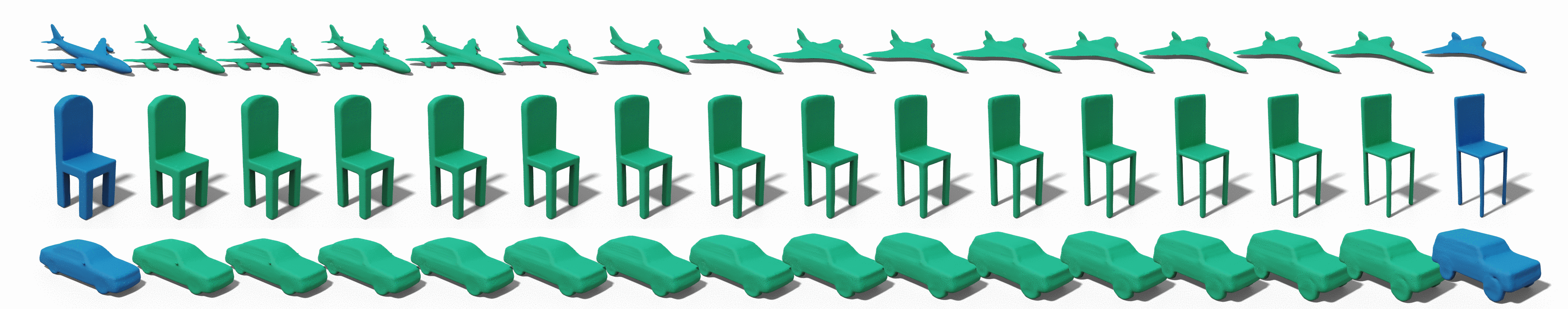
We show qualitative reconstruction results in Fig. 3. We compare our results with re-implemented OccNet. We also show shape interpolation results in Fig. 4. Interpolation is done by acquiring two features and from two different images. Then we reconstruct meshes while linearly interpolating the two features.
Ablation study.
We show the metrics under different hyper-parameter choices in Table 3, including different and . We find that generally smaller and larger gives better results. However when is small enough (), the metrics are very close no matter how large is.
Visualization of embedding space.
In Fig. 5, we first show along with the corresponding meshes. Since our embedding space is also , we can visualize the embedding space. When the number of points in is small, the embedded shape looks more like an ellipsoid. In this case, the Embedding Network maps inside points into an ellipsoid-like shape. When is getting larger, the embedded mesh has a shape more similar to the original one. Thus, the Embedding Network only shift points by a small distance. This shows how the Embedding Network and the Point Generation Network collaborate. Sometimes the Embedding Network does most of the work when points are difficult to classify, while sometimes the Point Generation Network needs to generate structured point sets. In Fig. 6, we show more examples of given and .
Relation to hypernetworks.
The approach of hypernetworks (Ha et al., 2016), uses a (hyper-)network to generate parameters of another network. Our method has a relation to hypernetworks. The final (decision) surface is decided by where is a point in . According to Eq. equation 6, the output is . The points is obtained by the Point Generation Network, which we can treat as a hypernetwork, and the points are generated parameters. Thus our method can also be interpreted as a hypernetwork. Littwin & Wolf (2019) proposes an approach for shape reconstruction with hypernetworks but with a very high-dimensional latent vector (1024) and generated parameters (3394), while we only use a 256 dimensional latent vector and parameters. We still have better results according to Table 2.
| IoU | 256 | 128 | 64 | 32 | 16 | 8 |
|---|---|---|---|---|---|---|
| Chamfer | 256 | 128 | 64 | 32 | 16 | 8 |
|---|---|---|---|---|---|---|
missing F-Score 256 128 64 32 16 8
![[Uncaptioned image]](/html/2010.08276/assets/images/points.png)
6 Conclusion
In this paper, we presented a shape representation for deep neural networks. Training data generating networks establish a connection between few-shot learning and shape representation by converting an image of a shape into a collection of points as training set for a supervised task. Training can be solved with meta-learning approaches for few-shot learning. While our solution is inspired by few-shot learning, it is different in: 1) our training datasets are generated by a separate network and not given directly; 2) our embedding network is conditioned on the task but traditional few-shot learning employs unconditional embedding networks; 3) our test dataset is generated by sampling and not directly given. The experiments are evaluated on a single image 3D reconstruction dataset and improve over the SOTA.
References
- Amos & Kolter (2017) Brandon Amos and J Zico Kolter. Optnet: Differentiable optimization as a layer in neural networks. In Proceedings of the 34th International Conference on Machine Learning-Volume 70, pp. 136–145. JMLR. org, 2017.
- Bertinetto et al. (2019) Luca Bertinetto, João F. Henriques, Philip H. S. Torr, and Andrea Vedaldi. Meta-learning with differentiable closed-form solvers. In 7th International Conference on Learning Representations, ICLR 2019, New Orleans, LA, USA, May 6-9, 2019. OpenReview.net, 2019. URL https://openreview.net/forum?id=HyxnZh0ct7.
- Chang et al. (2015) Angel X Chang, Thomas Funkhouser, Leonidas Guibas, Pat Hanrahan, Qixing Huang, Zimo Li, Silvio Savarese, Manolis Savva, Shuran Song, Hao Su, et al. Shapenet: An information-rich 3d model repository. arXiv preprint arXiv:1512.03012, 2015.
- Chen & Zhang (2019) Zhiqin Chen and Hao Zhang. Learning implicit fields for generative shape modeling. In Proceedings of the IEEE Conference on Computer Vision and Pattern Recognition, pp. 5939–5948, 2019.
- Chen et al. (2019) Zhiqin Chen, Andrea Tagliasacchi, and Hao Zhang. Bsp-net: Generating compact meshes via binary space partitioning. arXiv preprint arXiv:1911.06971, 2019.
- Choy et al. (2016) Christopher B Choy, Danfei Xu, JunYoung Gwak, Kevin Chen, and Silvio Savarese. 3d-r2n2: A unified approach for single and multi-view 3d object reconstruction. In European conference on computer vision, pp. 628–644. Springer, 2016.
- Crammer & Singer (2001) Koby Crammer and Yoram Singer. On the algorithmic implementation of multiclass kernel-based vector machines. Journal of machine learning research, 2(Dec):265–292, 2001.
- Deng et al. (2019) Boyang Deng, Kyle Genova, Soroosh Yazdani, Sofien Bouaziz, Geoffrey Hinton, and Andrea Tagliasacchi. Cvxnets: Learnable convex decomposition. arXiv preprint arXiv:1909.05736, 2019.
- Fan et al. (2017) Haoqiang Fan, Hao Su, and Leonidas J Guibas. A point set generation network for 3d object reconstruction from a single image. In Proceedings of the IEEE conference on computer vision and pattern recognition, pp. 605–613, 2017.
- Finn et al. (2017) Chelsea Finn, Pieter Abbeel, and Sergey Levine. Model-agnostic meta-learning for fast adaptation of deep networks. arXiv preprint arXiv:1703.03400, 2017.
- Genova et al. (2019) Kyle Genova, Forrester Cole, Daniel Vlasic, Aaron Sarna, William T Freeman, and Thomas Funkhouser. Learning shape templates with structured implicit functions. In Proceedings of the IEEE International Conference on Computer Vision, pp. 7154–7164, 2019.
- Gidaris & Komodakis (2018) Spyros Gidaris and Nikos Komodakis. Dynamic few-shot visual learning without forgetting. In Proceedings of the IEEE Conference on Computer Vision and Pattern Recognition, pp. 4367–4375, 2018.
- Gould et al. (2016) Stephen Gould, Basura Fernando, Anoop Cherian, Peter Anderson, Rodrigo Santa Cruz, and Edison Guo. On differentiating parameterized argmin and argmax problems with application to bi-level optimization. arXiv preprint arXiv:1607.05447, 2016.
- Groueix et al. (2018) Thibault Groueix, Matthew Fisher, Vladimir G Kim, Bryan C Russell, and Mathieu Aubry. A papier-mâché approach to learning 3d surface generation. In Proceedings of the IEEE conference on computer vision and pattern recognition, pp. 216–224, 2018.
- Ha et al. (2016) David Ha, Andrew Dai, and Quoc V Le. Hypernetworks. arXiv preprint arXiv:1609.09106, 2016.
- Hanocka et al. (2019) Rana Hanocka, Amir Hertz, Noa Fish, Raja Giryes, Shachar Fleishman, and Daniel Cohen-Or. Meshcnn: a network with an edge. ACM Transactions on Graphics (TOG), 38(4):1–12, 2019.
- Kendall et al. (2018) Alex Kendall, Yarin Gal, and Roberto Cipolla. Multi-task learning using uncertainty to weigh losses for scene geometry and semantics. In Proceedings of the IEEE Conference on Computer Vision and Pattern Recognition, pp. 7482–7491, 2018.
- Kingma & Ba (2014) Diederik P Kingma and Jimmy Ba. Adam: A method for stochastic optimization. arXiv preprint arXiv:1412.6980, 2014.
- Koch et al. (2015) Gregory Koch, Richard Zemel, and Ruslan Salakhutdinov. Siamese neural networks for one-shot image recognition. In ICML deep learning workshop, volume 2. Lille, 2015.
- Lee et al. (2019) Kwonjoon Lee, Subhransu Maji, Avinash Ravichandran, and Stefano Soatto. Meta-learning with differentiable convex optimization. In Proceedings of the IEEE Conference on Computer Vision and Pattern Recognition, pp. 10657–10665, 2019.
- Liang et al. (2017) Xiaodan Liang, Liang Lin, Yunchao Wei, Xiaohui Shen, Jianchao Yang, and Shuicheng Yan. Proposal-free network for instance-level object segmentation. IEEE transactions on pattern analysis and machine intelligence, 40(12):2978–2991, 2017.
- Lin et al. (2017) Chen-Hsuan Lin, Chen Kong, and Simon Lucey. Learning efficient point cloud generation for dense 3d object reconstruction. arXiv preprint arXiv:1706.07036, 2017.
- Littwin & Wolf (2019) Gidi Littwin and Lior Wolf. Deep meta functionals for shape representation. In Proceedings of the IEEE International Conference on Computer Vision, pp. 1824–1833, 2019.
- Lorensen & Cline (1987) William E Lorensen and Harvey E Cline. Marching cubes: A high resolution 3d surface construction algorithm. ACM siggraph computer graphics, 21(4):163–169, 1987.
- Mescheder et al. (2019) Lars Mescheder, Michael Oechsle, Michael Niemeyer, Sebastian Nowozin, and Andreas Geiger. Occupancy networks: Learning 3d reconstruction in function space. In Proceedings of the IEEE Conference on Computer Vision and Pattern Recognition, pp. 4460–4470, 2019.
- Michalkiewicz et al. (2019) Mateusz Michalkiewicz, Jhony K Pontes, Dominic Jack, Mahsa Baktashmotlagh, and Anders Eriksson. Deep level sets: Implicit surface representations for 3d shape inference. arXiv preprint arXiv:1901.06802, 2019.
- Murphy (2012) Kevin P Murphy. Machine learning: a probabilistic perspective, chapter 14.4.3. The MIT Press, 2012.
- Nichol et al. (2018) Alex Nichol, Joshua Achiam, and John Schulman. On first-order meta-learning algorithms. arXiv preprint arXiv:1803.02999, 2018.
- Novotny et al. (2018) David Novotny, Samuel Albanie, Diane Larlus, and Andrea Vedaldi. Semi-convolutional operators for instance segmentation. In Proceedings of the European Conference on Computer Vision (ECCV), pp. 86–102, 2018.
- Park et al. (2019) Jeong Joon Park, Peter Florence, Julian Straub, Richard Newcombe, and Steven Lovegrove. Deepsdf: Learning continuous signed distance functions for shape representation. In Proceedings of the IEEE Conference on Computer Vision and Pattern Recognition, pp. 165–174, 2019.
- Qi et al. (2017a) Charles R Qi, Hao Su, Kaichun Mo, and Leonidas J Guibas. Pointnet: Deep learning on point sets for 3d classification and segmentation. In Proceedings of the IEEE conference on computer vision and pattern recognition, pp. 652–660, 2017a.
- Qi et al. (2017b) Charles Ruizhongtai Qi, Li Yi, Hao Su, and Leonidas J Guibas. Pointnet++: Deep hierarchical feature learning on point sets in a metric space. In Advances in neural information processing systems, pp. 5099–5108, 2017b.
- Qiao et al. (2018) Siyuan Qiao, Chenxi Liu, Wei Shen, and Alan L Yuille. Few-shot image recognition by predicting parameters from activations. In Proceedings of the IEEE Conference on Computer Vision and Pattern Recognition, pp. 7229–7238, 2018.
- Ravi & Larochelle (2017) Sachin Ravi and Hugo Larochelle. Optimization as a model for few-shot learning. In 5th International Conference on Learning Representations, ICLR 2017, Toulon, France, April 24-26, 2017, Conference Track Proceedings. OpenReview.net, 2017. URL https://openreview.net/forum?id=rJY0-Kcll.
- Riegler et al. (2017) Gernot Riegler, Ali Osman Ulusoy, and Andreas Geiger. Octnet: Learning deep 3d representations at high resolutions. In Proceedings of the IEEE Conference on Computer Vision and Pattern Recognition, pp. 3577–3586, 2017.
- Sitzmann et al. (2020) Vincent Sitzmann, Eric R. Chan, Richard Tucker, Noah Snavely, and Gordon Wetzstein. Metasdf: Meta-learning signed distance functions. In Proc. NeurIPS, 2020.
- Snell et al. (2017) Jake Snell, Kevin Swersky, and Richard Zemel. Prototypical networks for few-shot learning. In Advances in neural information processing systems, pp. 4077–4087, 2017.
- Tan & Le (2019) Mingxing Tan and Quoc Le. Efficientnet: Rethinking model scaling for convolutional neural networks. In International Conference on Machine Learning, pp. 6105–6114. PMLR, 2019.
- Tancik et al. (2021) Matthew Tancik, Ben Mildenhall, Terrance Wang, Divi Schmidt, Pratul P Srinivasan, Jonathan T Barron, and Ren Ng. Learned initializations for optimizing coordinate-based neural representations. In Proceedings of the IEEE/CVF Conference on Computer Vision and Pattern Recognition, pp. 2846–2855, 2021.
- Tatarchenko et al. (2017) Maxim Tatarchenko, Alexey Dosovitskiy, and Thomas Brox. Octree generating networks: Efficient convolutional architectures for high-resolution 3d outputs. In Proceedings of the IEEE International Conference on Computer Vision, pp. 2088–2096, 2017.
- Tatarchenko et al. (2019) Maxim Tatarchenko, Stephan R Richter, René Ranftl, Zhuwen Li, Vladlen Koltun, and Thomas Brox. What do single-view 3d reconstruction networks learn? In Proceedings of the IEEE Conference on Computer Vision and Pattern Recognition, pp. 3405–3414, 2019.
- Vinyals et al. (2016) Oriol Vinyals, Charles Blundell, Timothy Lillicrap, Daan Wierstra, et al. Matching networks for one shot learning. In Advances in neural information processing systems, pp. 3630–3638, 2016.
- Wang et al. (2018) Nanyang Wang, Yinda Zhang, Zhuwen Li, Yanwei Fu, Wei Liu, and Yu-Gang Jiang. Pixel2mesh: Generating 3d mesh models from single rgb images. In Proceedings of the European Conference on Computer Vision (ECCV), pp. 52–67, 2018.
- Wang et al. (2017) Peng-Shuai Wang, Yang Liu, Yu-Xiao Guo, Chun-Yu Sun, and Xin Tong. O-cnn: Octree-based convolutional neural networks for 3d shape analysis. ACM Transactions on Graphics (TOG), 36(4):1–11, 2017.
- Wu et al. (2015) Zhirong Wu, Shuran Song, Aditya Khosla, Fisher Yu, Linguang Zhang, Xiaoou Tang, and Jianxiong Xiao. 3d shapenets: A deep representation for volumetric shapes. In Proceedings of the IEEE conference on computer vision and pattern recognition, pp. 1912–1920, 2015.
- Zhang & Wonka (2019) Biao Zhang and Peter Wonka. Point cloud instance segmentation using probabilistic embeddings. arXiv preprint arXiv:1912.00145, 2019.
Appendix A Appendix
A.1 Networks
We show the architecture of the embedding network and the points generator in Fig. 7. The embedding network is similar to DeepSDF (Park et al., 2019).
A.2 Visualization of feature space
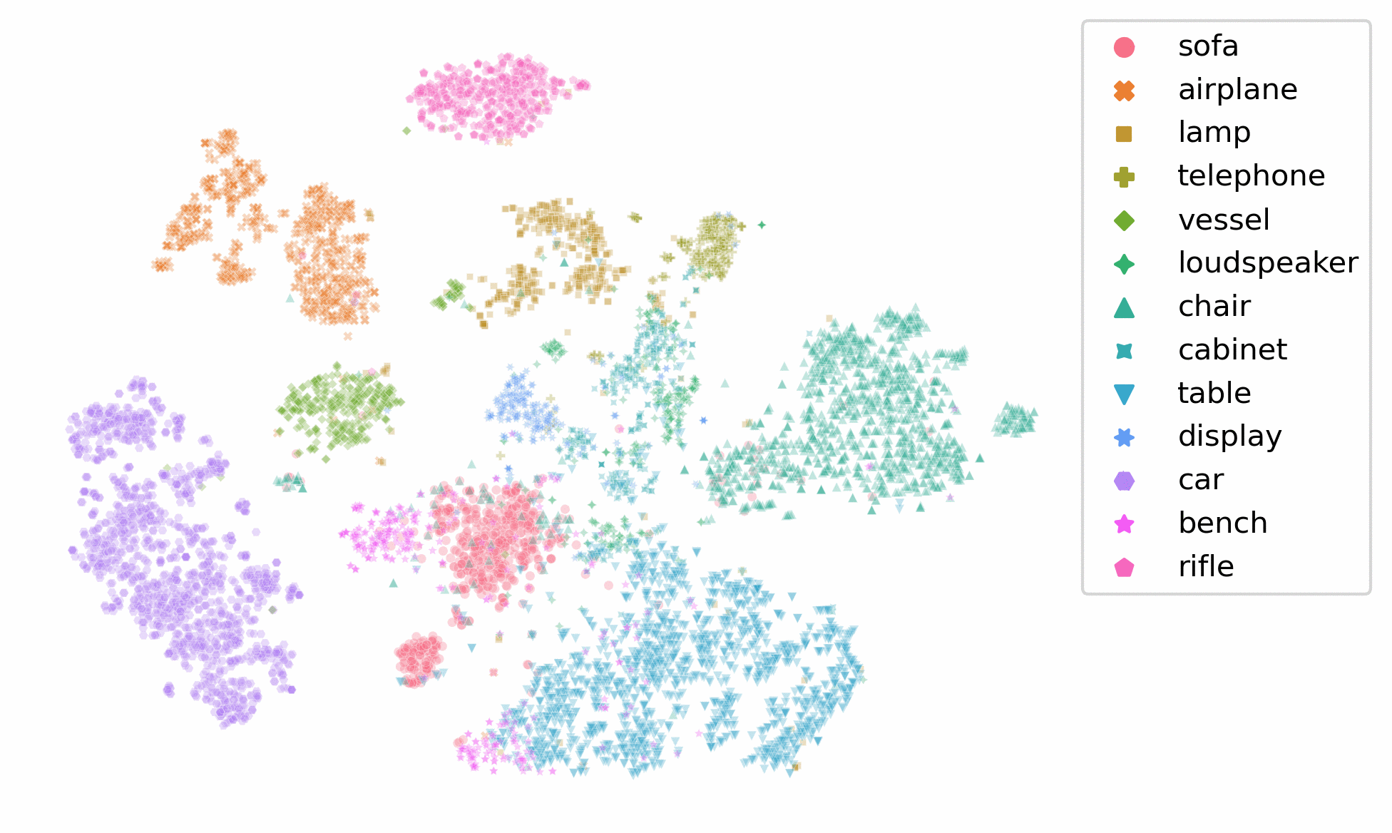
We visualize the feature space in Fig. 8.
A.3 Statistics of metrics
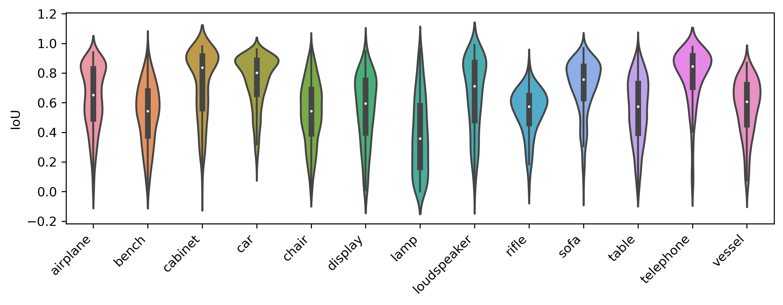
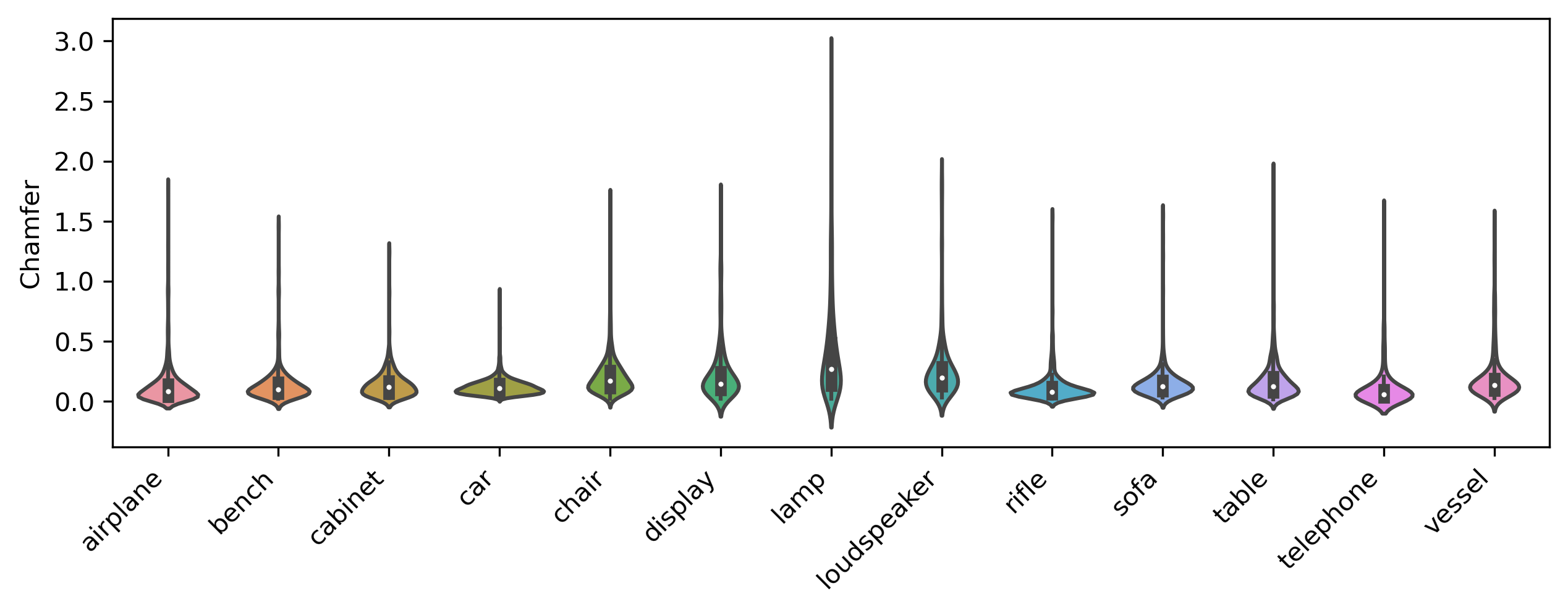
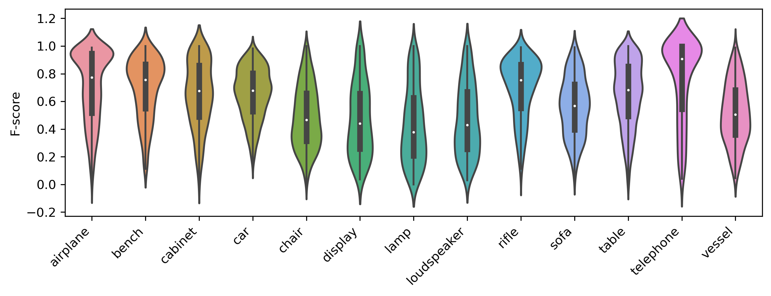
Here we show more detailed statistics in Fig. 9. Comparing to IoU and F-score, most of the values of Chamfer concentrate around the mean value and rare values very far from the mean. The “peakedness” property of Chamfer implies it is unstable to a certain extent. The conclusion is also consistent with Tatarchenko et al. (2019).
A.4 Shape Interpolation
In Fig. 10, we show reconstructed shapes with bilinear interpolation. Given shape latent feature vectors , , and , we show interpolated shapes with the bilinear interpolation equation
where and
| Category | IoU | Chamfer | F-Score | |||
|---|---|---|---|---|---|---|
| SVM | RR | SVM | RR | SVM | RR | |
| airplane | 0.639 | 0.633 | 0.117 | 0.121 | 71.87 | 71.15 |
| bench | 0.522 | 0.524 | 0.144 | 0.132 | 67.88 | 69.44 |
| cabinet | 0.731 | 0.732 | 0.139 | 0.141 | 65.15 | 65.33 |
| car | 0.745 | 0.748 | 0.119 | 0.121 | 65.77 | 65.48 |
| chair | 0.526 | 0.532 | 0.229 | 0.205 | 47.73 | 48.83 |
| display | 0.552 | 0.553 | 0.213 | 0.215 | 47.88 | 46.96 |
| lamp | 0.388 | 0.383 | 0.398 | 0.391 | 41.94 | 42.99 |
| loudspeaker | 0.662 | 0.658 | 0.252 | 0.247 | 46.95 | 46.86 |
| rifle | 0.536 | 0.540 | 0.112 | 0.111 | 69.18 | 69.40 |
| sofa | 0.700 | 0.707 | 0.158 | 0.155 | 55.40 | 56.40 |
| table | 0.538 | 0.551 | 0.193 | 0.171 | 64.03 | 65.25 |
| telephone | 0.776 | 0.779 | 0.101 | 0.106 | 76.60 | 75.96 |
| vessel | 0.563 | 0.567 | 0.177 | 0.186 | 51.38 | 51.57 |
| mean | 0.606 | 0.608 | 0.181 | 0.177 | 59.36 | 59.66 |
A.5 Effects of
In the main paper, we have a regularizer to force the embedding space to be similar to the original space,
| (10) |
When is very large, the embedding space is almost the same as the original space, especially when is large. The visualization is shown in Fig. 11. We set . This is much higher than recommended in the paper. In this case, we expect the embedding network to do less work and as reported for the method mainly works for a large number of points. We can observe that indeed the embedding space (bottom) is similar to the original space (top) especially when is large. Positive points are shown in red and negative points in blue. Top row: meshes are reconstructed with our regular pipeline. Generated points are fed into the Embedding Network first. Visualized points are in the original space. Middle row: meshes are reconstructed by removing the embedding network without re-training. This isn’t expected to work well. Generated points are directly used in generating classification boundaries. Visualized points are in the original space. We can see that even without the embedding network the results are surprisingly reasonable for a large number of points. Bottom row: meshes in the embedding space. Visualized points are in the embedding space. We can observe that the meshes look similar to the correct chair, especially for large . This also validates that the embedding network does not have a large influence on the result for large . If the regularizing weight is set to 0, the shape in embedding space will be more ellipsoid like.
Recall that, with the kernel ridge regression as our base learner, the final shape (decision) surface is decided by,
If the original and embedding space are close, we can even reconstruct meshes without the Embedding Network ,
The results are shown in Fig. 11.
A.6 The choice of base learners
In Table 4, we show results of different base learners, SVM and ridge regression. The difference between the two methods is very small.
A.7 Results on real world images
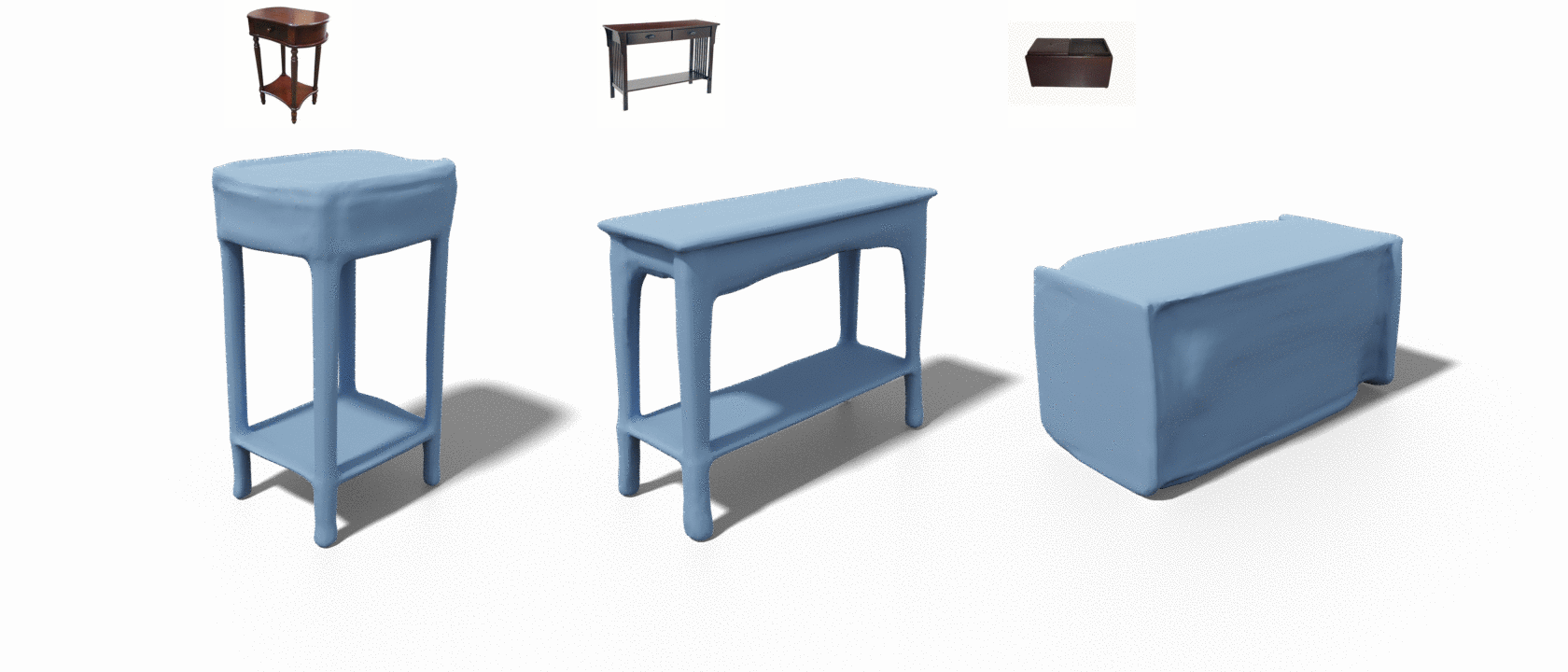
Note that our model is trained on a synthetic dataset (ShapeNet). Here we test how our model generalizes to real world datasets. Without retraining and fine-tuning, we apply our trained model to Stanford Online Products. The qualitative results are shown in Fig. 12. We believe that the results are good, but there is no ground truth data for evaluation.
A.8 Inter-Categories Interpolation
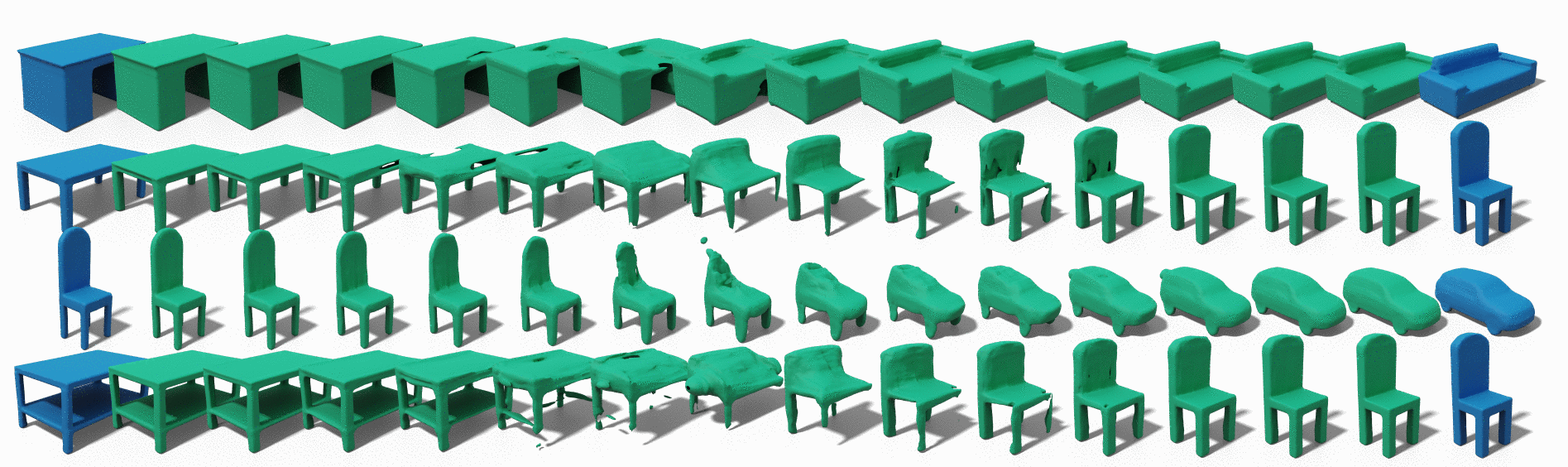
Similar to Fig. 4, we also show inter-categories interpolation in Fig. 13. We take samples from two different categories, and reconstruct shapes with interpolated latents. Although the interpolated shapes are not as high quality than the originals, they still show some characteristics of both categories, e.g., sofas which are as tall as tables, and cars with chair-leg-like tires.
A.9 Training and Inference
We describe the detailed training process in Algorithm 1. This algorithm can be viewed along with Fig. 2. We also show the full process how we generate a triangular mesh given an input image in Algorithm 2.
A.10 Choice of backbones
In Table 5, we show the performance of our method with different backbones. We keep all of the setup the same except for the feature backbone.
| Categ. | IoU | Chamfer | F-Score | |||||||||
|---|---|---|---|---|---|---|---|---|---|---|---|---|
| ENB1 | RN34 | RN50 | DN121 | ENB1 | RN34 | RN50 | DN121 | ENB1 | RN34 | RN50 | DN121 | |
| plane | 0.633 | 0.616 | 0.623 | 0.612 | 0.121 | 0.129 | 0.131 | 0.142 | 71.15 | 69.15 | 69.70 | 67.77 |
| bench | 0.524 | 0.506 | 0.500 | 0.508 | 0.132 | 0.135 | 0.152 | 0.145 | 69.44 | 67.24 | 65.69 | 66.32 |
| cabinet | 0.732 | 0.728 | 0.733 | 0.742 | 0.141 | 0.144 | 0.141 | 0.136 | 65.33 | 63.44 | 63.78 | 65.58 |
| car | 0.748 | 0.746 | 0.744 | 0.744 | 0.121 | 0.122 | 0.123 | 0.123 | 65.48 | 64.86 | 63.98 | 64.23 |
| chair | 0.532 | 0.520 | 0.521 | 0.532 | 0.205 | 0.213 | 0.219 | 0.216 | 48.83 | 47.33 | 47.14 | 48.11 |
| display | 0.553 | 0.549 | 0.534 | 0.554 | 0.215 | 0.209 | 0.222 | 0.210 | 46.96 | 46.45 | 43.83 | 46.85 |
| lamp | 0.383 | 0.378 | 0.370 | 0.386 | 0.391 | 0.399 | 0.434 | 0.410 | 42.99 | 41.38 | 39.49 | 41.81 |
| speaker | 0.658 | 0.647 | 0.647 | 0.659 | 0.247 | 0.262 | 0.265 | 0.252 | 46.86 | 44.47 | 43.77 | 46.52 |
| rifle | 0.540 | 0.521 | 0.515 | 0.504 | 0.111 | 0.124 | 0.118 | 0.124 | 69.40 | 67.19 | 66.47 | 65.09 |
| sofa | 0.707 | 0.691 | 0.694 | 0.702 | 0.155 | 0.164 | 0.166 | 0.155 | 56.40 | 54.32 | 54.18 | 55.62 |
| table | 0.551 | 0.535 | 0.532 | 0.550 | 0.171 | 0.177 | 0.200 | 0.176 | 65.25 | 63.92 | 63.26 | 65.22 |
| phone | 0.779 | 0.770 | 0.769 | 0.770 | 0.106 | 0.105 | 0.107 | 0.105 | 75.96 | 75.22 | 73.06 | 75.30 |
| vessel | 0.567 | 0.562 | 0.555 | 0.570 | 0.186 | 0.185 | 0.206 | 0.192 | 51.57 | 50.27 | 48.74 | 50.68 |
| mean | 0.608 | 0.598 | 0.595 | 0.602 | 0.177 | 0.182 | 0.191 | 0.183 | 59.66 | 58.10 | 57.16 | 58.39 |
A.11 Embedding dimensions
In Table 6, we show the performance of our method with different embeddings. Note that different from Table 5, the results shown here are trained with .
| Categ. | IoU | Chamfer | F-Score | |||||||||
|---|---|---|---|---|---|---|---|---|---|---|---|---|
| Spa | 32D | 64D | 128D | Spa | 32D | 64D | 128D | Spa | 32D | 64D | 128D | |
| plane | 0.637 | 0.627 | 0.630 | 0.624 | 0.119 | 0.125 | 0.132 | 0.123 | 71.54 | 70.67 | 70.91 | 70.30 |
| bench | 0.519 | 0.530 | 0.532 | 0.516 | 0.138 | 0.135 | 0.138 | 0.133 | 68.42 | 68.89 | 69.57 | 68.23 |
| cabinet | 0.744 | 0.735 | 0.739 | 0.736 | 0.135 | 0.136 | 0.138 | 0.134 | 66.54 | 66.92 | 67.13 | 66.77 |
| car | 0.747 | 0.746 | 0.749 | 0.746 | 0.119 | 0.121 | 0.118 | 0.119 | 65.51 | 65.53 | 65.98 | 65.50 |
| chair | 0.527 | 0.536 | 0.542 | 0.532 | 0.223 | 0.233 | 0.210 | 0.207 | 47.89 | 49.05 | 49.93 | 48.88 |
| display | 0.572 | 0.562 | 0.570 | 0.564 | 0.201 | 0.201 | 0.196 | 0.201 | 48.58 | 48.00 | 48.73 | 47.76 |
| lamp | 0.387 | 0.397 | 0.417 | 0.408 | 0.398 | 0.479 | 0.456 | 0.363 | 42.57 | 43.78 | 45.18 | 44.29 |
| speaker | 0.657 | 0.666 | 0.666 | 0.660 | 0.259 | 0.244 | 0.233 | 0.242 | 45.83 | 48.19 | 48.36 | 48.21 |
| rifle | 0.537 | 0.540 | 0.545 | 0.537 | 0.113 | 0.116 | 0.113 | 0.109 | 69.33 | 69.25 | 69.81 | 68.77 |
| sofa | 0.705 | 0.706 | 0.707 | 0.707 | 0.157 | 0.153 | 0.153 | 0.152 | 55.90 | 56.49 | 56.73 | 56.53 |
| table | 0.549 | 0.550 | 0.553 | 0.548 | 0.183 | 0.177 | 0.172 | 0.169 | 65.08 | 65.77 | 66.16 | 64.96 |
| phone | 0.779 | 0.780 | 0.786 | 0.777 | 0.107 | 0.100 | 0.094 | 0.097 | 76.95 | 76.83 | 76.29 | 76.06 |
| vessel | 0.575 | 0.572 | 0.577 | 0.569 | 0.189 | 0.199 | 0.189 | 0.183 | 51.75 | 52.10 | 52.03 | 51.84 |
| mean | 0.610 | 0.611 | 0.616 | 0.610 | 0.180 | 0.186 | 0.180 | 0.172 | 59.68 | 60.11 | 60.52 | 59.85 |