Fingerprinting Heatwaves and Cold Spells and Assessing Their Response to Climate Change using Large Deviation Theory
Abstract
Extreme events provide relevant insights into the dynamics of climate and their understanding is key for mitigating the impact of climate variability and climate change. By applying large deviation theory to a state-of-the-art Earth system model, we define the climatology of persistent heatwaves and cold spells in key target geographical regions by estimating the rate functions for the surface temperature, and we assess the impact of increasing CO2 concentration on such persistent anomalies. Hence, we can better quantify the increasing hazard due to heatwaves in a warmer climate. We show that two 2010 high impact events - summer Russian heatwave and winter Dzud in Mongolia - are associated with atmospheric patterns that are exceptional compared to the typical ones, but typical compared to the climatology of extremes. Their dynamics is encoded in the natural variability of the climate. Finally, we propose and test an approximate formula for the return times of large and persistent temperature fluctuations from easily accessible statistical properties.
Introduction
Understanding extreme events is a key scientific challenge and is essential for addressing the natural hazards due to climate variability and climate change. High-impact events are usually associated with long temporal persistence, as resilience against anomalous environmental conditions does not last indefinitely Easterling et al. (2000); Koppe et al. (2004); Poumadére et al. (2005); IPCC (2012). The theory of low-frequency variability of the atmosphere shows that long temporal persistence and large spatial extent of patterns go hand in hand Ghil and Robertson (2002); Ghil and Lucarini (2020). Let’s consider two high-impact climatic extremes that occurred in 2010. The summer Russian heatwave (RHW) had a temporal duration of about one month and a spatial extent of several million Km2 Barriopedro et al. (2011). The winter Mongolian Dzud (MD)- an extreme cold spell - affected Mongolia and a large part of Siberia also for about a month Rao et al. (2015); Sternberg (2018). Dzuds have historically been major drivers of migration for central Asian nomadic populations Fang and Liu (1992); Hvistendahl (2012). Persistent large scale atmospheric patterns can have a cascade effect Kornhuber et al. (2019): it is well known that the 2010 RHW was dynamically linked Hong et al. (2011); Lau and Kim (2012); Boschi and Lucarini (2019) to extensive floods in Pakistan.
Future changes in the statistics of heatwaves are worrying, as more persistent positive temperature fluctuations compound with the trend in the average temperature Seneviratne et al. (2006); Coumou et al. (2013); Pfleiderer et al. (2019); Kornhuber and Tamarin-Brodsky . Climate change leads to less frequent cold spells Smith and Sheridan (2020), even if specific dynamical processes might facilitate their occurrence Kretschmer et al. (2018); Cohen et al. (2018). Following Allen (2003), a lot of research has focused on understanding whether it is possible to attribute (and in which sense) individual extreme events to climate change Otto (2017), for defining science-based liability for their impacts. The attribution of the 2010 RHW to climate change has been heavily debated Dole et al. (2011); Rahmstorf and Coumou (2011); Otto et al. (2012).
This Letter
We aim at advancing our understanding of heatwaves and cold spells in the Northern Hemisphere (NH) and of their response to climate change. We treat the climate as a nonequilibrium system Lucarini et al. (2014, 2017); Ghil and Lucarini (2020) and analyze it with Large Deviation Theory Varadhan (1984); Touchette (2009); Dembo and Zeitouni (1998) (LDT).
LDT provides limit laws for the average of random variables, where stochasticity can also be due to deterministic chaos Kifer (1990). Let , where the ’s are identically distributed, possibly correlated, random variables. obeys a Large Deviation Principle (LDP) if exists. is the rate function (RF), quantifying the exponential decay of probabilities with for all , where , , and . To verify the existence of a LDP for an observable having integrated autocorrelation time Billingsley (2012) one can check whether
| (1) |
, converges for larger and larger multiples of the averaging time , where usually . In what follows both and are in units of days; see supplemental material (SM)111The SM is accessible at https://doi.org/10.6084/m9.figshare.14888151 and includes Refs. Osborn and Jones (2014); R Core Team (2016); Brockwell and Davis (2002).. LDT has been used to address some theoretical aspects of geophysical fluid dynamics Bouchet and Venaille (2012); Lucarini et al. (2014); Bouchet et al. (2019) but has been otherwise not yet widely used in climate studies. Ref. Ragone et al. (2017) investigates heatwaves by applying a genealogical algorithm to an intermediate complexity climate model; see also the recent follow-up work performed with a more complex climate model Ragone and Bouchet (2021). In Gálfi et al. (2019) we construct rate functions for surface temperature (ST) data using a highly-idealized atmospheric model.
Testing theories and methodologies across the model hierarchy is an effective research strategy in climate studies Held (2005); Ghil and Lucarini (2020). In this work, we perform for the first time LDT-based analysis on the outputs of a state-of-the-art CMIP6 Eyring et al. (2016) Earth system model (ESM), namely the MPI-ESM-LR model Giorgetta et al. (2013). CMIP6 models have provided key inputs for the preparation of the latest (6th) report of the Intergovernmental Panel for Climate Change (IPCC).
We have two closely related main objectives:
-
1.
we will attempt to establish LDPs for the ESM output in order to define an LDT-based geographical climatology of heatwaves and cold spells and investigate their sensitivity to concentration;
-
2.
we will use the ESM to look into the 2010 RHW and the much less studied MD, and argue that these events, while extreme, are in some sense typical and are part of the natural variability of the climate.
A key element to address point 2. is that LDT captures the least unlikely of all the unlikely ways a large and persistent fluctuation can occur den Hollander (2000). Let’s use a specific example that provides guidance for our analysis below. Hydrodynamic rogue waves can be explained using a LDP. As one takes sufficiently stringent height threshold criteria, the individual rogue waves become similar to each other, and their average converges to a special solution, associated with the so-called instanton Dematteis et al. (2019). This formalism can be extended for treating events that have long duration and high intensity Grafke and Vanden-Eijnden (2019), as in the case here.
Rate Functions for the Surface Temperature
We first analyze large deviations of the ST in a 1000-year long pre-industrial control run (namely with fixed greenhouse gases concentration and land-use) of the MPI-ESM-LR model Giorgetta et al. (2013). Building on the analysis of the climatic hot spots Giorgi (2006), we consider the following regions in the NH: Northwest, Southwest, and Southeast America; the Mediterranean; North Europe; Northwest and Northeast Asia; the North Atlantic; and the North Pacific. We analyze summer and winter ST separately, in order to have seasonal data with nearly stationary statistics. After removing the yearly cycle, we select for each year an extended summer - lasting days and beginning on May 5th - and an extended winter - lasting days and starting on December 1st, see SM for details.
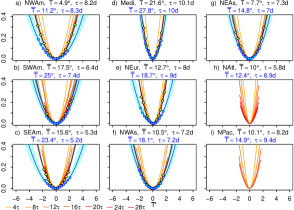
We estimate RFs via Eq. (1) for the spatially averaged ST in these regions and for the locales indicated in Fig. 1 of the SM. We compute for increasing averaging lengths . The optimal averaging block length is such that , Gálfi et al. (2019). We achieve convergence if . The RFs for the regions are steeper than those of the corresponding locales and their convergence is faster thanks to spatial averaging Gálfi et al. (2019), as shown in Figs. 2-7 of the SM. It is very encouraging to see that LDT seems applicable at different levels of spatial granularity also in an ESM with realistic geography. In all cases discussed below, the RFs are approximately quadratic. We will use this property at the end of the letter to present a preliminary example of the predictive power of our approach.
Figure 1 shows that for the summer RFs one finds convergence for the land areas and for the Mediterranean. The values of ranges between 1 and 2 months, which, encouragingly, corresponds with the time scale of actual high-impact heatwaves. The RFs are flatter for the North American and Eurasian regions, where a more continental climate with larger climate variability is observed, because a) the moderating effect of oceanic water masses is almost absent; and b) dry conditions can be more readily established and can lead to enhanced temperature fluctuations because of the reduced heat capacity of the soil.
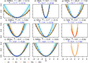
The winter RFs - Fig. 2 - are significantly flatter as an effect of the stronger atmospheric variability during winter; this is especially enhanced in continental regions, which feature large meridional temperature gradients Ghil and Robertson (2002), so that the corresponding RFs are very flat. As the Mediterranean has a weak seasonality, the winter and summer RF for the ST are quite similar. The optimal averaging length also in this case ranges approximately between one and two months, which is compatible with the time scale of cold spells in the real climate.
For both summer and winter ST, the RFs estimated for are very similar to those obtained by averaging over subsequent years, indicating that the LDP applies within a single season. Finally, no LDP can be found over the ocean for either season. The basic difference in our ability to define RFs for ST over land and ocean agrees with the presence of long-term memory for the ocean ST Fraedrich and Blender (2003); Zhu et al. (2010). Details on the convergence of the estimates of the RFs are shown in Figs. 8-9 of the SM.
Heatwaves and Cold Spells in a Warmer Climate
We can infer, at least qualitatively, the impact of climate change on the statistics of heatwaves and cold spells by comparing the previous RFs with those computed by analyzing the ST fields of a 140-year long steady state simulation run with quadrupled CO2 concentration. This corresponds to a much warmer and more equitable climate, with a globally averaged ST higher by about 6 K and greatly reduced ST difference between low and high latitudes. The RFs for summer - see Fig. 1 - are flatter in the Mediterranean and in all land regions, thus indicating an increased occurrence of heatwaves, also relative to much warmer average conditions. In some regions persistence is enhanced Kornhuber et al. (2019) as increases. The increase in the probability of occurrence of heatwaves can be attributed to the drying of the soil, which activates a complex set of positive feedbacks Seneviratne et al. (2006). Figure 2 shows that the winter RFs are everywhere steeper for the northern regions in the warmer climate, as the reduced ST difference between low and high latitudes leads to a weaker weather variability Screen (2014) due to the reduced thermodynamic climate efficiency Lucarini et al. (2014). Small changes are instead detected for the more southern regions. Hence, considering the average ST increase, one expects fewer and less damaging cold spells in the future Smith and Sheridan (2020). See further details on RFs for the 4CO2 simulation in the SM.
Fingerprinting the 2010 RHW and MD
Our idea here is to use the viewpoint by Dematteis et al. (2019); Grafke and Vanden-Eijnden (2019) briefly presented above for interpreting the 2010 RHW and MD. The corresponding monthly (August and January 2010, respectively) mean fields of climatological anomalies for the ST and 500 hPa geopotential height (GPH) are reconstructed using the NCEP-NCAR reanalysis Kanamitsu et al. (2002); see the SM for additional ST maps from observations. The GPH arguably provides the most relevant information on atmospheric dynamics at synoptic and planetary scales Ghil and Robertson (2002); Ghil and Lucarini (2020).
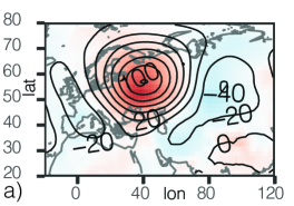
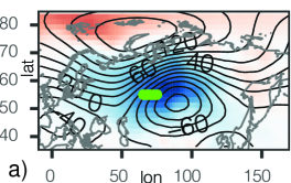
In order to investigate the RHW, we compute the mean anomaly fields for ST and GPH by averaging over the periods from the model run when we record ST anomalies K averaged over 30 days at the gridpoint located at (west of Moscow), which is in the core area of the 2010 event. Each of such periods (20 in total) corresponds to a heatwave. Size and duration of the fluctuations are chosen to match the observed one.
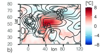
The composite fields performed by averaging over the 20 heatwaves - Fig. 3 a) - portray our estimate of the solution associated with the instanton. At large scales, these fields have a fair resemblance, both in shape and magnitude, with the observed anomalies for August 2010 (Fig. 3 b). We see a similar pattern of positive ST and GPH anomalies over an extended circular region containing the selected grid point. This pattern is more symmetric and longitudinally less extended than its counterpart in the reanalysis data. The spatial correlation between the fields is 0.54 (0.29) for ST (GPH), which is within the range of the value of spatial correlations computed between the individual heatwaves and their composite, which is () for the ST (GPH) field. Hence, the actual 2010 RHW can be seen as a fluctuation around the instantonic solution. See Figs. 10-11 in the SM and comments therein.
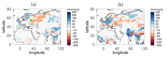
The full GPH field - see Fig. 10 in the SM - shows that the composite captures a pattern that resembles the strong blocking high that is the well-known cause of the 2010 RHW and, indeed, a (rarely) recurrent local climatic feature Dole et al. (2011). Looking at the monthly cumulative precipitation (Fig. 4), there is at least a qualitative agreement between the observed patterns of wet and dry anomalies (panel b) and the composite of the model data (panel a) in Europe, Western Siberia, parts of Africa, South, Southeast, and East Asia. Despite a fair agreement over South Asia, the very intense wet spot in the Upper Indus basin is missing. This is hardly surprising given the well-know difficulty of models in representing correctly the precipitation in that high-altitude locale Palazzi et al. (2015); Almazroui et al. (2020). Given the complexity of the processes associated with precipitation, these results are encouraging.
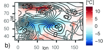
We proceed analogously for the 2010 MD. We look in the model dataset for events featuring deviations of ST K averaged over 30 days at the gridpoint located at N, 75 ° (east of Omsk), which belongs to the core of the recorded event. We find 24 of such events. The average fields of ST and GPH recorded during the large deviations of the local ST (Fig. 5 a) are in a fairly good agreement with the reanalysis data for January 2010 (Fig. 5 b). The spatial correlation coefficient between the corresponding anomaly fields is 0.80 (0.64) for ST (GPH). These figures are, again within the range of the values of the spatial correlations computed between the model composite and the 24 realised heatwaves, which is and for the ST and GPH fields, respectively. See also Figs. 12-13 in the SM and discussion therein. The spatial scale of ST anomalies for the MD extends throughout Eurasia, with a large core region in Siberia and northern Mongolia. The full 500 hPA GPH field shown in Fig. 12 of the SM shows that also here we can reconstruct the basic mechanism behind the cold spell: a cut-off low in East Asia that leads to advection of Arctic air into central Siberia.
Discussion and Outlook
We have provided a new outlook on heatwaves and cold spells in the NH by applying LDT to the output of a state-of-the-art ESM. Extreme and persistent ST fluctuations during winter and summer over land and over the Mediterranean obey LDPs. The properties of the RFs quantify the regional and seasonal differences in the probability of occurrence of persistent extreme ST anomalies. We can also better appreciate the future risk due to heatwaves, as the increase in the average ST comes together with increased probability of such persistent positive fluctuations.
The obtained RFs are approximately parabolic in the range of practical interest. Hence, the probability of observing an average anomaly of amplitude over a sufficiently long period of days is , where , where is the daily variance and is in days. We can estimate the probability of occurrence of events of amplitude and length relative to that of less extreme events of amplitude and length :
| (2) |
We have attempted a first test of Eq. 2 on the RHW and MD locales, starting from the return time of days moderate events, i.e. 1oC (-2oC) for the RHW (MD). We can predict accurately the return times of extreme events for days and days, see Fig. 14 in the SM. The formula applies a fortiori for lower-resolution time series (e.g. weekly/monthly averages). This idea, is promising for climate risk evaluation and deserves further study.
It is intriguing that the anomalies of the ST and GPH fields during the 2010 RHW (MD) event look rather similar to those constructed by looking at the summer warm (winter cold) model ST anomalies selected conditionally to the presence of a large deviation of ST at the chosen locale. One constructs a large-scale pattern that is involved in the occurrence of the persistent event: a blocking over Russia (a deep low in East Asia) for the RHW (MD). Using the conceptual framework proposed in Dematteis et al. (2019); Grafke and Vanden-Eijnden (2019), we claim that these extreme events (our results are stronger for the MD) are in fact typical - also at dynamical level, as part of the natural climate variability - once we use the statistical lens defined by LDPs, which identifies the reference instantons. Hence, they cannot be considered freak events or dragon kings Sornette and Ouillon (2012). Similar conclusions were drawn for the RHW in Dole et al. (2011) through a more empirical yet informative approach. Ref. Otto et al. (2012) suggested the absence of an a-priori dichotomy between attributing the 2010 RHW to natural climate variability Dole et al. (2011) or to climate change Rahmstorf and Coumou (2011). Indeed, while its dynamics is part of the natural climate variability, its probability of occurrence is modulated by the changing climate.
The viewpoint proposed in this paper possibly contributes to understanding the low-frequency variability of the atmosphere Ghil and Robertson (2002); Ghil and Lucarini (2020) and the role of stationary Rossby waves in causing extreme events Lau and Kim (2012); Kornhuber et al. (2019), and is the starting point for further investigations of specific case studies. In future work we will improve the quantitative evaluation of the agreement between observed extreme persistent observed and model-simulated events using tools like the Self Organizing Map Kohonen (2001). One also needs to test the robustness of our findings by intercomparing different models, given the uncertainties on the skill of ESMs in representing the low-frequency variability of the atmosphere Woollings et al. (2018) and its response to climate change Brown (2020).
Acknowledgements.
The authors thank D. Faranda, G. Messori, F. Ragone, A. Speranza, and J. Wouters for many exchanges on extreme events and acknowledge the support by DFG TRR181 (grant no. 274762653). VL thanks B. Hoskins for having stimulated this investigation and acknowledges the support by the H2020 project TiPES (grant no. 820970). The authors have equally contributed to this study.References
- Easterling et al. (2000) D. R. Easterling, G. A. Meehl, C. Parmesan, S. A. Changnon, T. R. Karl, and L. O. Mearns, Science 289, 2068 (2000), https://science.sciencemag.org/content/289/5487/2068.full.pdf .
- Koppe et al. (2004) C. Koppe, R. Sari Kovats, B. Menne, G. Jendritzky, W. H. O. R. O. for Europe, L. S. of Hygiene, T. Medicine, E. European Commission. Energy, S. Development, and D. Wetterdienst, “Heat-waves : risks and responses / by christina koppe … [et al.],” (2004).
- Poumadére et al. (2005) M. Poumadére, C. Mays, S. Le Mer, and R. Blong, Risk Analysis 25, 1483 (2005), https://onlinelibrary.wiley.com/doi/pdf/10.1111/j.1539-6924.2005.00694.x .
- IPCC (2012) IPCC, Managing the Risks of Extreme Events and Disasters to Advance Climate Change Adaptation (Cambridge Univerity Presse, 2012) [Field, C.B., V. Barros, T.F. Stocker, D. Qin, D.J. Dokken, K.L. Ebi, M.D. Mastrandrea,K.J. Mach, G.-K. Plattner, S.K. Allen, M. Tignor, and P.M. Midgley (eds.)]. A Special Report of Working Groups I and II of the Intergovernmental Panel on Climate Change.
- Ghil and Robertson (2002) M. Ghil and A. W. Robertson, Proceedings of the National Academy of Sciences 99, 2493 (2002), https://www.pnas.org/content/99/suppl_1/2493.full.pdf .
- Ghil and Lucarini (2020) M. Ghil and V. Lucarini, Rev. Mod. Phys. 92, 035002 (2020).
- Barriopedro et al. (2011) D. Barriopedro, E. M. Fischer, J. Luterbacher, R. M. Trigo, and R. García-Herrera, Science 332, 220 (2011), https://science.sciencemag.org/content/332/6026/220.full.pdf .
- Rao et al. (2015) M. P. Rao, N. Davi, R. arrigo, J. Skees, N. Baatarbileg, C. Leland, B. Lyon, S.-Y. Wang, and O. Byambasuren, Environmental Research Letters 10, 074012 (2015).
- Sternberg (2018) T. Sternberg, Natural Hazards 92, 27 (2018).
- Fang and Liu (1992) J.-Q. Fang and G. Liu, Climatic Change 22 (1992).
- Hvistendahl (2012) M. Hvistendahl, Science 337, 1596 (2012), http://www.sciencemag.org/content/337/6102/1596.full.pdf .
- Kornhuber et al. (2019) K. Kornhuber, S. Osprey, D. Coumou, S. Petri, V. Petoukhov, S. Rahmstorf, and L. Gray, Environmental Research Letters, 14, 054002 (2019).
- Hong et al. (2011) C.-C. Hong, H.-H. Hsu, N.-H. Lin, and H. Chiu, Geophysical Research Letters 38 (2011), 10.1029/2011GL047583, https://agupubs.onlinelibrary.wiley.com/doi/pdf/10.1029/2011GL047583 .
- Lau and Kim (2012) W. K. M. Lau and K.-M. Kim, Journal of Hydrometeorology 13, 392 (2012), https://journals.ametsoc.org/jhm/article-pdf/13/1/392/4110762/jhm-d-11-016_1.pdf .
- Boschi and Lucarini (2019) R. Boschi and V. Lucarini, Atmosphere 10, 489 (2019).
- Seneviratne et al. (2006) S. I. Seneviratne, D. Lüthi, M. Litschi, and C. Schär, Nature 443, 205 (2006).
- Coumou et al. (2013) D. Coumou, A. Robinson, and S. Rahmstorf, Climatic Change 118, 771 (2013).
- Pfleiderer et al. (2019) P. Pfleiderer, C.-F. Schleussner, K. Kornhuber, and D. Coumou, Nature Climate Change 9, 666 (2019).
- (19) K. Kornhuber and T. Tamarin-Brodsky, Geophysical Research Letters n/a, e2020GL091603, https://agupubs.onlinelibrary.wiley.com/doi/pdf/10.1029/2020GL091603 .
- Smith and Sheridan (2020) E. T. Smith and S. C. Sheridan, Geophysical Research Letters 47, e2020GL086983 (2020), e2020GL086983 2020GL086983, https://agupubs.onlinelibrary.wiley.com/doi/pdf/10.1029/2020GL086983 .
- Kretschmer et al. (2018) M. Kretschmer, D. Coumou, L. Agel, M. Barlow, E. Tziperman, and J. Cohen, Bulletin of the American Meteorological Society 99, 49 (2018), https://journals.ametsoc.org/bams/article-pdf/99/1/49/3754811/bams-d-16-0259_1.pdf .
- Cohen et al. (2018) J. Cohen, K. Pfeiffer, and J. A. Francis, Nature Communications 9, 869 (2018).
- Allen (2003) M. Allen, Nature 421, 891 (2003).
- Otto (2017) F. E. Otto, Annu. Rev. Environ. Resour. 42, 627 (2017).
- Dole et al. (2011) R. Dole, M. Hoerling, J. Perlwitz, J. Eischeid, P. Pegion, T. Zhang, X.-W. Quan, T. Xu, and D. Murray, Geophysical Research Letters 38 (2011), 10.1029/2010GL046582, https://agupubs.onlinelibrary.wiley.com/doi/pdf/10.1029/2010GL046582 .
- Rahmstorf and Coumou (2011) S. Rahmstorf and D. Coumou, Proceedings of the National Academy of Sciences 108, 17905 (2011), https://www.pnas.org/content/108/44/17905.full.pdf .
- Otto et al. (2012) F. E. L. Otto, N. Massey, G. J. van Oldenborgh, R. G. Jones, and M. R. Allen, Geophysical Research Letters 39 (2012), https://doi.org/10.1029/2011GL050422, https://agupubs.onlinelibrary.wiley.com/doi/pdf/10.1029/2011GL050422 .
- Lucarini et al. (2014) V. Lucarini, R. Blender, C. Herbert, F. Ragone, S. Pascale, and J. Wouters, Reviews of Geophysics 52, 809 (2014), https://agupubs.onlinelibrary.wiley.com/doi/pdf/10.1002/2013RG000446 .
- Lucarini et al. (2017) V. Lucarini, F. Ragone, and F. Lunkeit, Journal of Statistical Physics 166, 1036 (2017).
- Varadhan (1984) S. Varadhan, Large Deviations and Applications (SIAM, Philadelphia, 1984).
- Touchette (2009) H. Touchette, Physics Reports 478, 1 (2009).
- Dembo and Zeitouni (1998) A. Dembo and O. Zeitouni, Large Deviations Techniques and Applications, Applications of mathematics (Springer, New York, 1998).
- Kifer (1990) Y. Kifer, Transactions of the American Mathematical Society 321, 505 (1990).
- Billingsley (2012) P. Billingsley, Probability and Measure, Wiley Series in Probability and Statistics (Wiley, New York, 2012).
- Note (1) The SM is accessible at https://doi.org/10.6084/m9.figshare.14888151 and includes Refs. Osborn and Jones (2014); R Core Team (2016); Brockwell and Davis (2002).
- Bouchet and Venaille (2012) F. Bouchet and A. Venaille, Physics Reports 515, 227 (2012), statistical mechanics of two-dimensional and geophysical flows.
- Bouchet et al. (2019) F. Bouchet, J. Rolland, and E. Simonnet, Physical Review Letters 122, 074502 (2019).
- Ragone et al. (2017) F. Ragone, J. Wouters, and F. Bouchet, Proceedings of the National Academy of Sciences (2017), 10.1073/pnas.1712645115, https://www.pnas.org/content/early/2017/12/18/1712645115.full.pdf .
- Ragone and Bouchet (2021) F. Ragone and F. Bouchet, (2021), arXiv:2009.02519, arXiv:2009.02519 [physics.ao-ph] .
- Gálfi et al. (2019) V. M. Gálfi, V. Lucarini, and J. Wouters, Journal of Statistical Mechanics: Theory and Experiment 2019, 033404 (2019).
- Held (2005) I. M. Held, Bull. Am. Met. Soc. 86, 1609 (2005).
- Eyring et al. (2016) V. Eyring, S. Bony, G. A. Meehl, C. A. Senior, B. Stevens, R. J. Stouffer, and K. E. Taylor, Geoscientific Model Development 9, 10539 (2016).
- Giorgetta et al. (2013) M. A. Giorgetta, J. Jungclaus, C. H. Reick, S. Legutke, J. Bader, M. Böttinger, V. Brovkin, T. Crueger, M. Esch, K. Fieg, K. Glushak, V. Gayler, H. Haak, H.-D. Hollweg, T. Ilyina, S. Kinne, L. Kornblueh, D. Matei, T. Mauritsen, U. Mikolajewicz, W. Mueller, D. Notz, F. Pithan, T. Raddatz, S. Rast, R. Redler, E. Roeckner, H. Schmidt, R. Schnur, J. Segschneider, K. D. Six, M. Stockhause, C. Timmreck, J. Wegner, H. Widmann, K.-H. Wieners, M. Claussen, J. Marotzke, and B. Stevens, Journal of Advances in Modeling Earth Systems 5, 572 (2013), https://agupubs.onlinelibrary.wiley.com/doi/pdf/10.1002/jame.20038 .
- den Hollander (2000) F. den Hollander, Large Deviations (American Mathematical Society, 2000).
- Dematteis et al. (2019) G. Dematteis, T. Grafke, M. Onorato, and E. Vanden-Eijnden, Phys. Rev. X 9, 041057 (2019).
- Grafke and Vanden-Eijnden (2019) T. Grafke and E. Vanden-Eijnden, Chaos: An Interdisciplinary Journal of Nonlinear Science 29, 063118 (2019).
- Giorgi (2006) F. Giorgi, Geophysical Research Letters 33 (2006), 10.1029/2006GL025734, https://agupubs.onlinelibrary.wiley.com/doi/pdf/10.1029/2006GL025734 .
- Fraedrich and Blender (2003) K. Fraedrich and R. Blender, Phys. Rev. Lett. 90, 108501 (2003).
- Zhu et al. (2010) X. Zhu, K. Fraedrich, Z. Liu, and R. Blender, Journal of Climate 23, 5021 (2010), https://journals.ametsoc.org/jcli/article-pdf/23/18/5021/3975143/2010jcli3370_1.pdf .
- Screen (2014) J. A. Screen, Nature Climate Change 4, 577 (2014).
- Kanamitsu et al. (2002) M. Kanamitsu, W. Ebisuzaki, J. Woollen, S.-K. Yang, J. J. Hnilo, M. Fiorino, and G. L. Potter, Bulletin of the American Meteorological Society Nov 2002, 1631 (2002).
- Palazzi et al. (2015) E. Palazzi, J. von Hardenberg, S. Terzago, and A. Provenzale, Climate Dynamics 45, 21 (2015).
- Almazroui et al. (2020) M. Almazroui, S. Saeed, F. Saeed, M. N. Islam, and M. Ismail, Earth Systems and Environment 4, 297 (2020).
- Sornette and Ouillon (2012) D. Sornette and G. Ouillon, The European Physical Journal Special Topics 205, 1 (2012).
- Kohonen (2001) T. Kohonen, Self-organizing maps, Springer series in information sciences, 30 (Springer, Berlin, 2001).
- Woollings et al. (2018) T. Woollings, D. Barriopedro, J. Methven, S.-W. Son, O. Martius, B. Harvey, J. Sillmann, A. R. Lupo, and S. Seneviratne, Current Climate Change Reports 4, 287 (2018).
- Brown (2020) S. J. Brown, Weather and Climate Extremes 30, 100278 (2020).
- Osborn and Jones (2014) T. J. Osborn and P. D. Jones, Earth System Science Data 6, 61 (2014).
- R Core Team (2016) R Core Team, R: A Language and Environment for Statistical Computing, R Foundation for Statistical Computing, Vienna, Austria (2016).
- Brockwell and Davis (2002) P. Brockwell and R. Davis, Introduction to Time Series and Forecasting, Srpinger texts in statistics (Springer, New York, 2002).