SI: Nanoscale Rigidity in Cross-Linked Micelle Networks Revealed by XPCS Nanorheology

I Rheology Measurements

The viscoelastic nature of the OMCA-CTAB micelle solution is evident in the complex moduli (Fig. 1). The solid line shows a fit with the standard Maxwell model where the storage and loss modulus as a function of the shear frequency, $\omega$, are given by

$$G^{\prime}(\omega) =G_{0}\dfrac{\tau_{R}^{2}\omega^{2}}{1+\omega^{2}\tau_{R}^{2}}\ \quad\text{storage modulus}\,,$$ (1)

$$G^{\prime\prime}(\omega) =G_{0}\dfrac{\tau_{R}\omega}{1+\omega^{2}\tau_{R}^{2}}\ \quad\text{loss modulus}\,,$$ (2)

$\tau_{R}$ is the terminal stress relaxation time and $G_{0}$ is the plateau modulus.

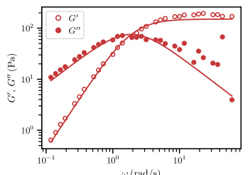
Figure 1: Complex moduli of a $200\text{\,}\mathrm{m\textsc{M}}$ OMCA-CTAB solution. The storage and loss modulus, ${G^{\prime},\,G^{\prime\prime}}$, are fitted with the standard Maxwell model (solid lines).

II XPCS Measurement Protocol

The OMCA-CTAB system is very susceptible to radiation damage and a certain illuminated volume of the sample can only stand a limited radiation dose before the properties are altered by the X-rays. To study possible effects of the X-ray beam on the sample dynamics, time resolved correlation functions are calculated as a function of the absorbed dose, $\mathcal{D}$, during a measurement:

$$c_{2}(q,\mathcal{D}_{1},\mathcal{D}_{2})=\frac{\langle I(q,\mathcal{D}_{1})I(q,\mathcal{D}_{2})\rangle_{p}}{\langle I(q,\mathcal{D}_{1})\rangle_{p}\langle I(q,\mathcal{D}_{2})\rangle_{p}}\,.$$ (3)

Figure 2(b) displays $c_{2}((q,\mathcal{D}_{1},\mathcal{D}_{2}))$ measured with $100\text{\,}\mathrm{nm}$ silica nanoparticles in a $50\text{\,}\mathrm{m\textsc{M}}$ OMCA-CTAB solution. Cuts parallel to the diagonal (marked in different shades of blue) are plotted as a function of the absorbed dose in Figure 2(a) and normalized to the initial contrast. After roughly $10\text{\,}\mathrm{kGy}$, the contrast drops steeply indicating that the X-rays are damaging the micelle network resulting in an acceleration of the dynamics. To be on the safe side, a maximum dose of $2\text{\,}\mathrm{kGy}$ was chosen for the XPCS measurements.

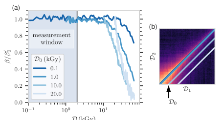
Figure 2: (a) The normalized contrast is extracted from diagonal cuts of the time resolved correlation function (b) as a function of the absorbed dose during a measurement, ${\mathcal{D}_{1},\,\mathcal{D}_{2}}$. A measurement window up to $2\text{\,}\mathrm{kGy}$ is chosen to safely exclude beam damage effects in the XPCS measurements.

III Determination Of Dynamical Parameters

Fig. 1 in the letter shows that for the shortest exposure time of $40\text{\,}\mathrm{\SIUnitSymbolMicro s}$ the scattered intensity is reduced to less than $1\text{\times}{10}^{-2}$ photons per pixel. This requires many repetitions to increase the signal-to-noise ratio of a set of correlation functions. For instance the correlation functions shown in Fig. 2 in the main text are calculated from ca. two million speckle patterns.

Additionally, a global fitting scheme was used for the parameter estimation. The dynamical parameters $\xi,\,D_{i},\,\alpha_{i},\,n_{i}$ and $\Gamma_{0}$ are calculated by globally fitting a dataset of correlation functions (all available $q$-bins) with the double exponential model for ${g_{2}(q,t)}$ introduced in the letter. The residuals are minimized by a Levenberg-Marquardt algorithm. The parameters describing the structural relaxation were considered as free fitting parameters. Let $N_{q}$ be the number of $q$-bins, then the parameters of the structural relaxation are ${\alpha_{2}^{1}\dots\alpha_{2}^{N_{q}}}$ and ${\Gamma_{2}^{1}\dots\Gamma_{2}^{N_{q}}}$. The exponent $n_{2}$ is determined by fitting ${\Gamma_{2}(q)=D_{2}q^{n_{2}}}$. To fit the fast relaxation mode the $q$-dependence of the short-time dispersion relation is modeled by ${\Gamma_{1}(q)=\Gamma_{0}+D_{1}q^{n_{1}}}$ resulting in a reduced number of fit parameters. Consequently, $\Gamma_{0}$, $D_{1}$ and $n_{1}$ are inferred directly from the correlation functions.

Figure 3: Correlation plot of the $q$-scaling exponent, $n$, and the KWW-exponent, $\alpha$. The color distinguishes between the short- and long-time relaxation. The solid gray line indicates ${n=2/\alpha}$. The data points corresponding to the correlation functions shown in the manuscript are annotated.

The parameters $n_{2}$ and the average $\alpha_{2}$ are inversely proportional to each other as shown in Fig. 3 in blue. Their relation can be described by

$$n_{i}=2/\alpha_{i}\,,$$ (4)

as indicated by the gray line. In general, the two relaxation processes can only be resolved with sufficient time resolution and when they are well separated. In addition to the data shown in the main text where these conditions are fulfilled Fig. 3 contains additional datasets where the fast relaxation process could not be resolved to emphasize the generality of Eq. (4). Eq. (4) is explicitly used in the fits of the short-time behavior.

The reliability of the estimation of $\Gamma_{0}$ is evident in Fig. 4. The figures show the mutual dependency of the fit parameters. Clearly, the constant low-$q$ plateau $\Gamma_{0}$ can be estimated independently from ${D_{1},\,n_{1}}$ which demonstrates the robustness of the fit.

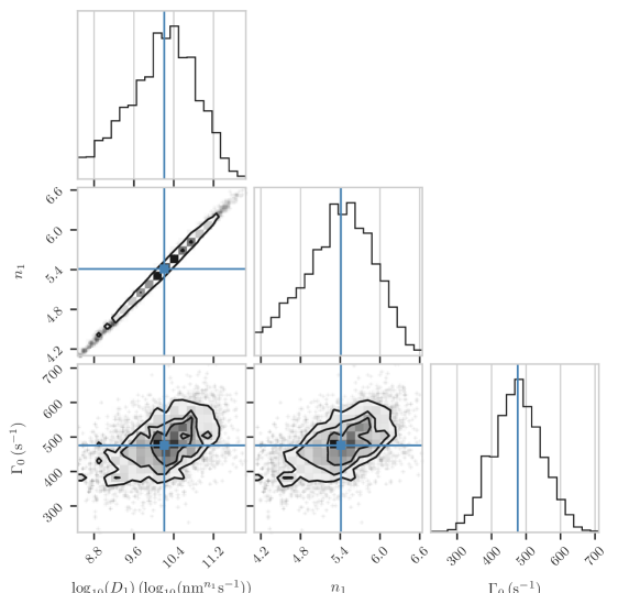
Figure 4: Posterior probability distributions (histograms) and mutual correlation plots (others) between fit parameters. The solid lines in the correlation plots indicate $25\text{\,}\mathrm{\char 37\relax}50\text{\,}\mathrm{\char 37\relax}75\text{\,}\mathrm{\char 37\relax}$. The blue lines indicate the maximum likelihood solution of each parameter. The fits are performed with the correlation functions shown in Fig. 2 in the letter.