Training Flexible Depth Model by Multi-Task Learning
for Neural Machine Translation

Abstract

The standard neural machine translation model can only decode with the same depth configuration as training. Restricted by this feature, we have to deploy models of various sizes to maintain the same translation latency, because the hardware conditions on different terminal devices (e.g., mobile phones) may vary greatly. Such individual training leads to increased model maintenance costs and slower model iterations, especially for the industry. In this work, we propose to use multi-task learning to train a flexible depth model that can adapt to different depth configurations during inference. Experimental results show that our approach can simultaneously support decoding in 24 depth configurations and is superior to the individual training and another flexible depth model training method——LayerDrop.

1 Introduction

As neural machine translation models become heavier and heavier Vaswani et al. (2017), we have to resort to model compress techniques (e.g., knowledge distillation Hinton et al. (2015); Kim and Rush (2016)) to deploy smaller models in devices with limited resources, such as mobile phones. However, a practical challenge is that the hardware conditions of different devices vary greatly. To ensure the same calculation latency, customizing distinct model sizes (e.g., depth, width) for different devices is necessary, which leads to huge model training and maintenance costs Yu et al. (2019). For example, we need to distill the pre-trained large model into N individual small models. The situation becomes worse for the industry when considering more translation directions and more frequent model iterations.

An ideal solution is to train a single model that can run in different model sizes. Such attempts have been explored in SlimNet Yu et al. (2019) and LayerDrop Fan et al. (2020). SlimNet allows running in four width configurations by joint training of these width networks, while LayerDrop can decode with any depth configuration by applying Dropout Srivastava et al. (2014) on layers during training.

In this work, we take a further step along the line of flexible depth network like LayerDrop. As shown in Figure 1, we first demonstrate that when there is a large gap between the predefined layer dropout during training and the actual pruning ratio during inference, LayerDrop’s performance is poor. To solve this problem, we propose to use multi-task learning to train a flexible depth model by treating each supported depth configuration as a task. We reduce the supported depth space for the aggressive model compression rate and propose an effective deterministic sub-network assignment method to eliminate the mismatch between training and inference in LayerDrop. Experimental results on deep Transformer Wang et al. (2019) show that our approach can simultaneously support decoding in 24 depth configurations and is superior to the individual training and LayerDrop.

2 Flexible depth model and LayerDrop

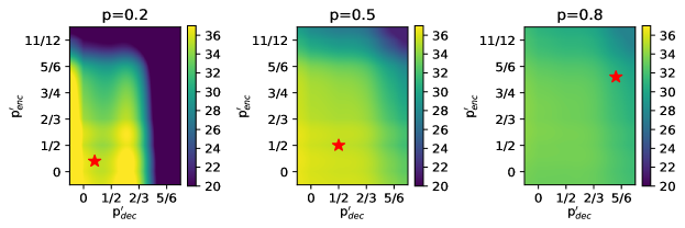
Figure 1: BLEU score heatmaps of a 12-layer encoder and a 6-layer decoder model trained by LayerDrop with different layer dropout $p$. p${}_{enc}^{\prime}$ and p${}_{dec}^{\prime}$ denote the layer-prunning ratio at inference on encoder and decoder, respectively. For example, p${}_{enc}^{\prime}$=11/12 means decoding by one encoder layer without the other 11 encoder layers. The red star marks the training layer dropout, i.e. p${}_{enc}^{\prime}$=p${}_{dec}^{\prime}$=p.

2.1 Flexible depth model

We first give the definition of flexible depth model (FDM): given a neural machine translation model $\mathcal{M}_{M-N}$ whose encoder depth is $M$ and decoder depth is $N$, in addition to (M,N), if $\mathcal{M}_{M-N}$ can also simultaneously decode with different depth configurations $(m_{i},n_{i})_{i=1}^{k}$ where $m_{i}\leq M$ and $n_{i}\leq N$ and obtain the comparable performance with independently trained model $\mathcal{M}_{m_{i}-n_{i}}$, we refer to $\mathcal{M}_{M-N}$ as a flexible depth model with a capacity of $k$. We notice that although a pre-trained vanilla Transformer can force decoding with any depth, its performance is far behind the independently trained model . Therefore, the vanilla Transformer does not belong to FDM.

2.2 LayerDrop

In NMT, both encoder and decoder are generally composed of multiple layers with residual connections, which can be formally described as:

$$x_{i+1}=x_{i}+\textrm{Layer}(x_{i}).$$ (1)

To make the model robust to pruned layers (shallower networks), LayerDrop proposed by Fan et al. (2020), applies structured dropout over layers during training. A Bernoulli distribution associated with a pre-defined parameter $p\in$ [0,1] controls the drop rate. It modifies Eq. 1 as:

$$x_{i+1}=x_{i}+Q_{i}*\textrm{Layer}(x_{i})$$ (2)

where $Pr(Q_{i}=0)=p$ and $Pr(Q_{i}=1)=1-p$. In this way, the $l$-th layer theoretically can take any proceeding layer as input, rather than just the previous one layer ($l-1$-th layer).

At runtime, given the desired layer-pruning ratio $p^{\prime}=1-D_{inf}/D$ where $D_{inf}$ is the number of layers actually used in decoding and $D$ is the total number of layers, LayerDrop selects to remove the $d$-th layer such that:

$$d\equiv 0(\textrm{mod}\lfloor\frac{1}{p^{\prime}}\rfloor)$$ (3)

2.3 LayerDrop’s problem for flexible depth

Although LayerDrop can play a good regularization effect when training deep Transformer Fan et al. (2020), we argue that this method is not suitable for FDM. As illustrated in Figure 1, we demonstrate that LayerDrop suffers a lot when there is a large gap between the pre-defined layer dropout $p$ in training and the actual pruning ratio $p^{\prime}$ at runtime. We attribute it to two aspects:

1. Huge sub-network space in training. Consider a D-layer network, because each layer can be masked or not, up to $2^{D}$ sub-networks are accessible during training, which is a major challenge when D is large.

2. Mismatch between training and inference. As opposite to training, LayerDrop uses a deterministic sub-network at inference when given the layer pruning ratio $p^{\prime}$ (See Eq. 3), which leads to a mismatch between training and inference. For example, for D=6 and D_inf=3, there are $\tbinom{D}{D_{inf}}$ sub-network candidates during training, while only one of them is used in decoding.

3 Flexible depth by multi-task learning

1

2pre-train $\mathcal{M}_{M-N}$ on training data $\mathcal{D}$;

3 generate distillation data $\mathcal{D}^{\prime}$ by $\mathcal{M}_{M-N}$;

4 $\mathcal{M}^{\prime}_{M-N}\leftarrow\mathcal{M}_{M-N}$;

5

6for $t$ in $1,2,\ldots,T$ do

7       $\mathcal{B}\leftarrow$ sample batch from $\mathcal{D}^{\prime}$ ;

8       gradient $\mathcal{G}\leftarrow 0$;

9       for  ($m_{i}$, $n_{i}$) in $\hat{\phi}(M)\otimes\hat{\phi}(N)$  do

10            

11            $\textrm{SN}_{e}$, $\textrm{SN}_{d}$ $\leftarrow\mathcal{F}(m_{i},M)$, $\mathcal{F}(n_{i},N)$;

12             Feed $\mathcal{B}$ into network $(\textrm{SN}_{e},\textrm{SN}_{d})$;

13             Collect gradient $g$ by Back-Propa.;

14             $\mathcal{G}\leftarrow\mathcal{G}+g$;

15            

16       end for

17      Optimize $\mathcal{M}^{\prime}_{M-N}$ with gradient $\mathcal{G}$;

18      

19 end for

Return $\mathcal{M}^{\prime}_{M-N}$

Algorithm 1 Training Flexible Depth Model by Multi-Task Learning.

We propose to use multi-task learning to solve the above problems. All tasks are trained jointly and share the same parameters. Concretely, unlike LayerDrop, which allows up to $M\times N$ possible depth configurations, our approach sets a smaller depth configuration space $(m_{i},n_{i})_{i=1}^{k}(k<M\times N)$ in advance and takes each $(m_{i},n_{i})$ as a task. Another major difference from LayerDrop is that each task’s sub-network is unique and deterministic in our method, resulting in consistent sub-network used between training and inference.

1. Reduce depth space. For depth D, in principle, LayerDrop can be pruned to any depth of $\phi(D)=\{0,1,2,\ldots,D\}$. However, consider the actual situation of model compression for resource-limited devices, it is unnecessary if the compressing rate is too low, e.g., $D$ $\rightarrow$ $D$-1. Therefore, for an aggressive compress rate, we replace the entire space $\phi(D)$ with the set of all positive divisors of $D$ :

   $$\hat{\phi}(D)=\{d|D\%d=0,1\leq d\leq D\}$$ (4)

   The physical meaning of $\hat{\phi}(D)$ is to compress every $D/d$ layers into one layer, where $d\in$ $\hat{\phi}(D)$.

2. Guideline for deterministic sub-network assignment. The use of deterministic sub-networks is critical to maintaining the consistency between training and inference. However, for each $d\in\hat{\phi}(D)$, it is not trivial to decide which $d$ layers should be selected to construct the $d$-layer sub-network. Here we propose two metrics to guide the procedure. The first is task balance (TB), whose motivation is to make every layer have as uniform tasks as possible. We use the standard deviation of the number of tasks per layer to measure it quantitatively:

   $$\textrm{TB}=\sqrt{\frac{\sum_{i\in[1,D]}{\Big{(}t(i)-\bar{t}\Big{)}^{2}}}{D}}$$ (5)

   where $t(i)$ is the number of tasks in which the $i$-th layer participates and $\bar{t}=\frac{\sum_{d\in\hat{\phi}(D)}{d}}{D}$. The second is average layer distance (ALD), which requires the distance between adjacent layers in the sub-network $\textrm{SN}(d)=\{L_{a_{1}},L_{a_{2}},\ldots,L_{a_{d}}\}$ should be large. For example, for a 6-layer network, if we want to build a 2-layer sub-network, it is unreasonable to select $\{L_{1},L_{2}\}$ directly because the features extracted by adjacent layers are semantically similar Peters et al. (2018); Raganato and Tiedemann (2018). Therefore, we use the average distance between layers in all sub-networks as the metric:

   $$\textrm{ALD}=\frac{\sum\limits_{d\in\hat{\phi}(D)}{\sum\limits_{a_{i},a_{i+1}\in\textrm{SN}(d)}{|a_{i+1}-a_{i}|}}}{Z}$$ (6)

   where $Z=\sum_{d\in\hat{\phi}(D)}{(d-1)}$ is the normalization item.

3. Proposed method. Guided by these two metrics, we design an effective sub-network assignment method Optimal. We record the usage state $s_{i}$ of each layer to ensure not to put too many tasks on the same layer. At initialization, we set $s_{i}$ as Alive. For $d\in\hat{\phi}(D)$, Optimal prioritizes to process large depth. Optimal uniformly assigns one layer for every $c=D/d$ layers to make ALD high. In each chunk, we pick the middle layer of $\textrm{ceil}(c/2)-1$ (called MiddleLeft). Note that, LayerDrop uses the leftmost layer in each chunk (called Left), as shown in Eq. 3. Although Left and MiddleLeft have the same ALD, we found that there is a large gap in TB. For example, when $D$=12, Left’s TB is 1.5, which is much higher than MiddleLeft’s 0.78 (lower is better). Then, Optimal records which layers are used and picks the less used layers as much as possible. Each used layer is marked as Dead. If current alive layers cannot accommodate the picked depth $d$, we pass it and choose a smaller $d$ until the alive layers are sufficient, or reset all layers as Alive.

   	1			2			3			6
   	Base	$\Delta_{LD}$	$\Delta_{MT}$	Base	$\Delta_{LD}$	$\Delta_{MT}$	Base	$\Delta_{LD}$	$\Delta_{MT}$	Base	$\Delta_{LD}$	$\Delta_{MT}$
   1	31.54	-3.04	-0.09	33.38	-2.37	+2.67	33.87	-1.99	+0.64	34.77	-2.27	-0.03
   2	32.80	-0.98	+0.31	34.15	-0.53	+0.48	34.58	-0.22	+0.55	34.95	-0.15	+0.49
   3	33.38	-0.40	+0.26	34.40	+0.15	+0.65	34.74	+0.40	+0.75	35.29	+0.25	+0.52
   4	33.92	-0.27	+0.44	34.77	+0.38	+0.59	35.01	+0.50	+0.86	35.37	+0.41	+0.68
   6	34.28	-0.29	+0.07	35.06	+0.20	+0.42	35.23	+0.41	+0.61	35.51	0.34	+0.51
   12	34.72	-0.05	+0.06	35.26	+0.49	+0.53	35.52	+0.53	+0.44	35.74	+0.49	+0.48

   Table 1: BLEU scores of Baseline/LayerDrop/MT in all tasks (6$\times$4). $\Delta_{LD}$/$\Delta_{MT}$ represents the BLEU score difference between LayerDrop/MT and Baseline, respectively. All the three methods have the same training cost. Boldface denotes the winner.

4. Training. Algorithm 1 describes the training process of our method. During training, compared with individual training and LayerDrop from scratch, our FDM finetunes on the individually pre-trained $\mathcal{M}_{M-N}$ and uses sequence-level knowledge distillation (Seq-KD) Kim and Rush (2016) to help shallower networks training. We note that in conventional Seq-KD, the student model cannot finetune on the teacher model directly because the two models have different sizes. However, FDM allows models with different depths to share the same parameters, and finetuning on the pre-trained teacher model also promotes model convergence.

4 Experiments

4.1 Setup

System	w/o Seq-KD	w/ Seq-KD
Baseline	33.92	34.51
LayerDrop	32.80	34.18
MT	34.07	34.95

Table 2: Average BLEU scores of 24 tasks on test set w.r.t. Seq-KD.

We conducted experiments on IWSLT’14 German$\rightarrow$English (De$\rightarrow$En, 160k) following the same setup as Wu et al. (2019). To verify FDM’s efficiency, we train all models with a deep encoder to contain more tasks. Specifically, we train a PreNorm Transformer Wang et al. (2019) with M=12 and N=6. See Appendix A for the details.

We mainly compare our method MT with the two baselines: Baseline and LayerDrop. Baseline denotes individually training the standard Transformer from scratch with different depths. For fair comparisons, both Baseline and LayerDrop use Seq-KD during training and have the same training costs .

4.2 Results and Analysis

1. Main results. As shown in Table 1, we compared Baseline, LayerDrop and our MT in all tasks. Although LayerDrop outperforms our method when a few layers pruned, we can see that MT is the winner in most tasks (20/24). It indicates that our method is superior to LayerDrop for FDM training and demonstrates the potential to substitute a dozen models with different depths to just one model. Besides, in line with Fan et al. (2020), it is interesting to see the FDM without any pruning outperforms the individually trained model (see M=12, N=6), which is obvious evidence that jointly training of various depth models has a good regularization effect.

2. Knowledge distillation. Table 2 shows average BLEU scores of 24 tasks when training a flexible depth model with/without Seq-KD. It is clear that using distillation data helps FDM training in all systems, which is in line with the previous single-model compression study Kim and Rush (2016). According to Zhou et al. (2020), Seq-KD makes the training data distribution smoother, so we suspect that FDM benefits from Seq-KD because of the difficulty of multi-task learning.

   Strategy	TB$\downarrow$	ALD$\uparrow$	BLEU6×4
   Head	1.78	1.0	34.37
   Seq	0.49	1.0	34.53
   Left	1.50	2.0	34.59
   MiddleLeft	0.78	2.0	34.90
   Optimal	0.49	2.05	34.95

   Table 3: Average BLEU scores of 24 tasks on test set w.r.t. sub-network strategy. We report TB and ALD on encoder side. $\downarrow$ denotes the lower the better, while $\uparrow$ is on contrary. Note that, unlike the standard BLEU score, $\textrm{BLEU}_{6\times 4}$ is more difficult to change significantly because it is scaled of the number of tasks.

3. Sub-layer assigiment strategy. Besides the proposed Optimal and Left used by LayerDrop and its improved version MiddleLeft, we also compared with the other two strategies: Head and Seq, to check the consistency between BLEU and the proposed guidelines (TB and ALD). Head is the simplest method, which always picks the first $d$ layers as the sub-network. However, it causes the bottom layers heavier than the top layers. Seq avoids this problem by sequentially skipping previously used layers. For example, for $D$=6, $d$=1, Seq first uses $L_{1}$ as the sub-network. Next, when $d=2$, Seq selects $L_{2}$ and $L_{3}$. This method ensures that the minimal burden on all layers, but it violates the ALD metrics. Table 3 shows the average BLEU scores on all tasks by several sub-network strategies. While MiddleLeft already has good TB and ADL, we argue that it is not the best. This is because MiddleLeft treats each $d$ independently regardless of which layers are used in the previous $d^{\prime}$. We can see the proposed policy with lower TB and higher ALD obtains the best result, which indicates that our proposed metrics are helpful to determine which strategy is sound.

   System	# task	$\textrm{BLEU}_{N=6}$	$\textrm{BLEU}_{M=12}$
   Baseline	1	35.27	35.31
   MT (only encoder)	6	35.79	N/A
   MT (only decoder)	4	N/A	35.80
   MT (both)	24	35.71	35.68

   Table 4: Average BLEU scores when reducing the number of tasks.

4. Reduce the number of tasks. Intuitively, the number of tasks demines the learning difficulty of our method. To verify this assumption, we tested the other two baselines: (1) only training the flexible-depth encoder (depth from {1, 2, 3, 4, 6, 12}) but the decoder depth is the constant 6, denoted by MT (only encoder); (2) only training the flexible-depth decoder (depth from {1, 2, 3, 6}) but the encoder depth is the constant 12, denoted by MT (only decoder). Then we compared the average BLEU scores under fixing the decoder depth as 6 ($\textrm{BLEU}_{N=6}$) and fixing the encoder depth as 12 ($\textrm{BLEU}_{M=12}$). As shown in Table 4, when we reduce the number of tasks, we can generally obtain better performance. It indicates that if removing some unnecessary tasks, our FDM has the potential for further improvement.

   Burden	Batch	#Enc.	#Dec.	BLEU6×4
   100%	$B$	6	4	34.95
   50%	$B$	6	2	34.79
   	$B$	3	4	34.74
   	0.5$B$	6	4	34.77
   25%	$B$	6	1	34.67
   	$B$	3	2	34.58
   	0.5$B$	6	2	34.51
   	0.5$B$	3	4	34.54
   	0.25$B$	6	4	34.52

   Table 5: BLEU scores against training efficiency. $B$ denotes the full token-level batch size of 8k. $\textrm{BLEU}_{6\times 4}$ represents the average BLEU scores on 24 tasks.

5. Training efficiency. Our multi-task learning needs to accumulate gradients on all tasks, and its cost is linearly related to the number of tasks. Actually, we can sample fewer tasks instead of enumerating them all. For example, randomly sampling 3 tasks from 6 depth candidates (denoted by #Enc.=3). Another way to reduce training costs is to use smaller batches. We compared different strategies at {100%, 50%, 25%} training costs, as shown in Table 5. First of all, we can see that more training costs can obtain better performance. Compared with reducing tasks and reducing batches, we found that the former is a better choice. In particular, sampling more depths on the encoder side is more important than the decoder side, which is consistent with the recent observation in Wang et al. (2019) that encoder is more important than decoder in terms of translation performance.

5 Conclusion

We demonstrated LayerDrop is not suitable for FDM training because of (1) the huge sub-network space in training and (2) the mismatch between training and inference. Then we proposed to use multi-task learning to mitigate it. Experimental results show that our approach can decode with up to 24 depth configurations and obtain comparable or better performance than individual training and LayerDrop. In the future, we plan to explore more effective FDM training methods, and combining flexible depth and width is also one of the attractive directions.

Appendix A Detailed training setup

We replicate the model configuration (embed=512, ffn=1024, head=4) as the baseline in (Wu et al., 2019). In addition, the batch size of 8192, attention dropout of 0.1, and relu dropout of 0.1 is used as suggested by Wang et al. (2019). When training the standard Transformer from scratch, we follow the inverse_sqrt learning rate schedule with learning rate of 0.0015 and warmup of 8k. To speed up convergence of FDMs (e.g. MT, LayerDrop), all of them are finetuned from the pre-trained baseline with learning rate of 0.0005 and warmup of 4k.

At inference, we use a beam size of 5 and average last 5 checkpoints. We use case insensitive BLEU score evaluated by multi-bleu.perl as previous works.

References

- Fan et al. (2020) Angela Fan, Edouard Grave, and Armand Joulin. 2020. Reducing transformer depth on demand with structured dropout. In ICLR 2020 : Eighth International Conference on Learning Representations.
- Hinton et al. (2015) Geoffrey Hinton, Oriol Vinyals, and Jeff Dean. 2015. Distilling the knowledge in a neural network. arXiv preprint arXiv:1503.02531.
- Kim and Rush (2016) Yoon Kim and Alexander M Rush. 2016. Sequence-level knowledge distillation. In Proceedings of the 2016 Conference on Empirical Methods in Natural Language Processing, pages 1317–1327.
- Peters et al. (2018) Matthew Peters, Mark Neumann, Mohit Iyyer, Matt Gardner, Christopher Clark, Kenton Lee, and Luke Zettlemoyer. 2018. Deep contextualized word representations. In Proceedings of the 2018 Conference of the North American Chapter of the Association for Computational Linguistics: Human Language Technologies, Volume 1 (Long Papers), volume 1, pages 2227–2237.
- Raganato and Tiedemann (2018) Alessandro Raganato and Jörg Tiedemann. 2018. An analysis of encoder representations in transformer-based machine translation. In Proceedings of the 2018 EMNLP Workshop BlackboxNLP: Analyzing and Interpreting Neural Networks for NLP, pages 287–297, Brussels, Belgium.
- Srivastava et al. (2014) Nitish Srivastava, Geoffrey Hinton, Alex Krizhevsky, Ilya Sutskever, and Ruslan Salakhutdinov. 2014. Dropout: a simple way to prevent neural networks from overfitting. The journal of machine learning research, 15(1):1929–1958.
- Vaswani et al. (2017) Ashish Vaswani, Noam Shazeer, Niki Parmar, Jakob Uszkoreit, Llion Jones, Aidan N Gomez, Łukasz Kaiser, and Illia Polosukhin. 2017. Attention is all you need. In Advances in Neural Information Processing Systems, pages 6000–6010.
- Wang et al. (2019) Qiang Wang, Bei Li, Tong Xiao, Jingbo Zhu, Changliang Li, Derek F. Wong, and Lidia S. Chao. 2019. Learning deep transformer models for machine translation. In Proceedings of the 57th Annual Meeting of the Association for Computational Linguistics, pages 1810–1822, Florence, Italy.
- Wu et al. (2019) Felix Wu, Angela Fan, Alexei Baevski, Yann N. Dauphin, and Michael Auli. 2019. Pay less attention with lightweight and dynamic convolutions. In 7th International Conference on Learning Representations, ICLR 2019.
- Yu et al. (2019) Jiahui Yu, Linjie Yang, Ning Xu, Jianchao Yang, and Thomas Huang. 2019. Slimmable neural networks. In ICLR 2019 : 7th International Conference on Learning Representations.
- Zhou et al. (2020) Chunting Zhou, Jiatao Gu, and Graham Neubig. 2020. Understanding knowledge distillation in non-autoregressive machine translation. In ICLR 2020 : Eighth International Conference on Learning Representations.