Quantum computing approach to railway dispatching and conflict management optimization on single-track railway lines

Abstract

In this work, we consider a practical railway dispatching problem: delay and conflict management on a single-track railway line. We examine the issue of train dispatching consequences caused by the arrival of an already delayed train to the segment being considered. This problem is computationally hard and often needs to be solved timely. Here, we introduce a quadratic unconstrained binary optimization (QUBO) model of the problem in question, compatible with the emerging quantum annealing technology. The model’s instances can be executed on present-day quantum annealers. As a proof-of-concept, we solve selected real-life problems from the Polish railway network using D-Wave quantum annealers. As a reference, we also provide solutions calculated with classical methods, including those relevant to the community (linear integer programming) and a sophisticated algorithm based on tensor networks for solving QUBO problems.

Keywords

Railway dispatching problem, train delay management, railway conflict management, quadratic unconstrained binary optimization (QUBO), quantum annealing, adiabatic quantum computing, quantum-inspired algorithms, tensor networks.

1 Introduction

Railway operations involve a broad range of scheduling activities, ranging from operational train dispatching to provisional timetable planning in case of disturbances. Many of these tasks require solving computationally expensive and overall challenging combinatorial problems. Various consequences of incorrect dispatching decisions can be severe in terms of resources (e.g., time costs, passengers’ satisfaction, financial loss).

Due to the importance of solving optimization problems, particularly those requiring nearly real-time solutions, new computing devices are being developed. Many of these devices rely on quantum systems, and their calibrations may depend on algorithms motivated by these systems. Moreover, novel hardware such as the D-Wave quantum annealer promises to deliver scalability beyond current classical hardware limitations. However, they often require a different mathematical modeling framework. For instance, the aforementioned annealer accepts an Ising spin glass instance as its input and outputs solutions encoded in spin configurations. High-quality solutions are expected to be computed by these devices in a reasonable time, even for larger problems (currently, up to $5000$ variables on a sparse graph [1]).

A priori it is unknown which spin configuration encodes the optimal solution, and the number of possible combinations is enormous (i.e., $2^{5000}\approx 10^{1666}$) [2]. Brute-force searching through all configurations in a reasonable time is possible only for small systems. It takes roughly two weeks to exhaustively find the low-energy spectrum of a general Ising Hamiltonian with only $50$ spins, even incorporating massive parallelization techniques [3]. In comparison, the typical time scale of the annealer runtime is milliseconds even for large instances [4]. Nevertheless, there is additional time needed for pre- and post-processing of data. Moreover, to increase the probability of finding the optimal solution, the experiment must typically be repeated multiple times.

Last but not least, today’s annealing devices are still prone to errors. Hence, most experiments involving annealing processors produce results that are far from theoretical predictions. However, this is expected to change in the not too distant future as the annealing technology is advancing rapidly. Moreover, various efficient algorithms have been developed in the past few decades to tackle problems relevant to statistical and solid-state physics. These sophisticated methods can also be incorporated to solve quadratic unconstrained binary optimization (QUBO).

To what extent real-life QUBO instances will be challenging for near-term quantum annealers and classical heuristic algorithms remains to be seen. Here, we provide, first and foremost, a proof-of-concept demonstrating how current quantum annealers and physics-inspired methods can tackle real-life dispatching problems. In particular, we solve the delay and conflict management on an existing Polish railway, whose real-time solution is of paramount importance for the local community.

2 Literature review

In this Section we survey the literature background of our work, both regarding the railway dispatching problem and quantum annealing.

2.1 Railway dispatching problem on single-track lines

Railway dispatching problem management is quite a complex area of transportation research. Here we focus on the delay management on single-track railways. This problem concerns the operative modifications of train paths upon disturbances in the railway traffic. Incorrect decisions may cause the dispatching situation to deteriorate further by propagating the delay, resulting in unforeseeable consequences. Henceforth, we discuss this problem’s details and survey some literature on the topic. Although we focus on single-track railway lines, some considerations may also be applicable to multi-track railways.

2.1.1 Problem description

Consider a part of a railway network in which the traffic is affected by a disturbance. As a result, some trains cannot run according to the original timetable. Hence, a new, feasible timetable should be created promptly, minimizing unwanted consequences of the delay.

To be more specific, we are given a part of a railway network (referred to as the network). This network is divided into block sections. The latter is understood as a railway network section that can be occupied by only one train at a time. We focus on single-track railway lines. These include passing sidings (referred to as sidings): parallel tracks, typically at stations, where trains heading in opposite directions can meet and pass (M-P). Similarly, trains heading in the same directions can meet and overtake (M-O). There are multiple ways of including sidings in the model, which we will describe shortly. The implications of an adverse decision can be severe in terms of the time needed to reach subsequent sidings.

All trains run according to a timetable. We assume that the initial timetable is conflict free and that is meets all the feasibility criteria. The criteria may vary [5, 6] depending on the railway network in question. The possible variants include technical requirements such as speed limits, dwell times, and other signaling-imposed requirements, as well as rolling stock circulation criteria, and passenger demands for trains to meet. By a conflict we refer to the inadmissible situation in which at least two trains are supposed to occupy the same block section.

The railway delay management problem can be viewed from various perspectives, including that of a passenger, the infrastructure manager, or a transport operation company [5, 6, 7]. Here, we look at this problem from the perspective of the infrastructure manager, who is to make the ultimate decision about the modifications and is in the position to prioritize the requirements.

In what follows, we assume that – for whatever reason – a delay occurs. Hence, some trains’ locations differ from the scheduled ones. The objective is to redesign the timetable to avoid conflicts and minimize delays. Note that the overall delay of a train is the sum of two types of delays. A primary delay is caused by the initial disturbance (at some point on the railway line) and the fact that there is a minimal amount of time needed to reach further destinations where the delay is considered (e.g., due to speed limits). This delay is unavoidable even in a situation in which no other trains are present on the network and the whole infrastructure can serve that single train. The primary delay provides a lower bound on the overall delay. The delay of a train beyond the primary delay is called the secondary delay. It can be non-zero if there are conflicts to be resolved by dispatching, and it can be minimized by making optimal decisions. The optimization goal is to minimize some function of secondary delays, e.g., their maximum or a weighted sum. Note that there are many other practically relevant options for the objective function [8], e.g. the total passenger delay or the cost of operations, and some of these are also in line with our approach.

The mathematical treatment of railway delay and conflict management leads to NP-hard problems; certain simple variants are NP-complete [9]. It is broadly accepted that these problems are equivalent to job-shop models with blocking constraints [10], given the release and due dates of the jobs and depending on the requirements of the model and additional constraints such as recirculation or no-wait. The correspondence between the metaphors is the following. Trains are the jobs and block sections are the machines. Concerning the objective functions, the (weighted) total tardiness or make-span is typically addressed, which is the (weighted) sum of secondary delays or the minimum of the largest secondary delay in the railway context. So with the standard notation of scheduling theory [11], our problem falls into the class $J_{m}|r_{i},d_{i},block|\sum_{j}w_{j}T_{j}$.

2.1.2 Existing approaches

The following summary of railway dispatching and conflict management is focused on the works that are closely related to the problem addressed by us. A more comprehensive review of the huge literature on optimization methods applicable to railway management problems can be found in many related publications, notably [6, 8, 12, 13, 14, 15, 16].

On a single-track line, the possible actions that can be taken to reschedule trains are the following: allocating new arrival and departure times, changing tracks and platforms, and reordering the trains by adjusting the meet-and-pass plans [17, 6, 8]. An important issue in modeling single-track lines is the handling of sidings (stations). As pointed out in [18], there are three approaches:

• Parallel machine approach, in which its is assumed that each track (in our notation, station block) within the siding corresponds to a separate machine in the job shop, thereby losing the possibility of flexible routing i.e., changing track orders at a station afterward.

• Machine unit approach, in which parallel tracks (block sections) are treated as additional units of the same machine.

• Buffer approach, in which sidings at the same location are handled as buffers without internal structure, therefore not warranting the feasibility of track occupation planning at a station.

As to the nature of the decision variables, two major classes of models may be identified:

• Order and precedence variables prescribe the order in which a machine processes jobs, i.e., the order of trains passing a given block section in the railway dispatching problem on single-track lines.

• Discrete time units, in which the decision variables belong to discretized time instants; the binary variables describe whether or not the event happens at a given time.

These two approaches lead to different model structures, which are hard to compare. The discrete time units approach appears to be more suitable for a possible QUBO formulation, but it leads to a large number of decision variables and thus worse scaling. On the other hand, the order and precedence variables approach can lead to a representation of the problem with alternative graphs [19, 20], which is an intuitive picture. The solution of this problem representation leads to mixed-integer programs that can possibly be solved with iterative methods (such as branch-and-bound), which makes them unsuitable for a reformulation to QUBO. Time-indexed variables, on the other hand, can result in pure binary problems that can be transformed into QUBOs [21], so we follow the latter approach.

Returning to [18], the considered problem with the parallel machine approach, machine unit approach, and order and precedence variables approach is – in all cases – denoted as $J_{m}|r_{i},d_{i},block,rcrc|\sum_{j}T_{j}$ when using the standard notation of scheduling theory set out in [11]. In comparison, in the present work will adopt slightly different constraints and objectives, namely, $J_{m}|r_{i},d_{i},block|\sum_{j}w_{j}T_{j}$. As to decision variables, we opt for discrete time units and time-indexed variables. (For the sake of completeness, we demonstrate that the problem can also be encoded with precedence variables and handled by a linear solver).

In [22], Zhou and Zhong considered the problem of timetabling on a single-track line. The starting times of trains and their stops are given, and a feasible schedule is to be designed to minimize the total running time of (typically passenger) trains. Although their problem, notably its objective function and the input, is different, the constraints are similar to those of our problem. The authors also deal with conflicts, dwell times, and minimum headway times for entering a segment of the railway line. They handle the problem with reference to resource-constrained project scheduling. Their decision variables are the discretized entry and leave times of the trains at the track segments, binary precedence variables describing the order of the trains passing a track segment, and time-indexed binary variables describing the occupancy of a segment by a given train at a given time. They introduce a branch-and-bound procedure with an efficiently calculable conflict-based bound in the bounding step to supplement the commonly used Lagrangian approach. They demonstrate its applicability to scheduling of up to $30$ passenger trains for a $24$-hour periodic planning horizon on a line with $18$ stations in China.

Harrod [23] proposed a discrete-time railway dispatching model, with a focus on conflict management. In this work, the train traffic flow is modeled as a directed hypergraph, with hyperarcs representing train moves with various speeds. This may be confined to an integer programming model with time-, train-, and hypergraph-related variables and a complex objective function covering multiple aspects. The model is demonstrated on an imaginary single-track line with long passing sidings at even-numbered block sections of up to 19 blocks in length. An intensive flow of trains at moderate speeds is examined. The model instances are solved by CPLEX in the order of 1000 seconds of computation time. As a practical application, a segment of a busy North American mainline is used, on which the model produced practically useful results. Bigger examples were also experimented with, leading to the conclusion that the approach is promising but that it needs more specialized technology than a standard mixed-integer programming (MIP) solver to be efficient.

Meng and Zhou [24] describe a simultaneous train rerouting and rescheduling model based on network cumulative flow variables. Their model also employs discrete-time-indexed variables. They implement a Lagrangian relaxation solution algorithm and make detailed experiments showing that their approach performs promisingly on a general n-track railway network. In the introduction of their article they tabulate numerous timetabling and dispatching algorithms.

This brief survey of the extensive literature confirms that the problem of railway dispatching and conflict management is indeed a good candidate for demonstrating new computational technology capable of solving hard problems. Only a very few models have been put into practice. The size and complexity of realistic dispatching problems make it challenging for the models to solve them with current computational technology.

2.2 Quantum annealing and related methods

Let us now turn our attention to the main tools used in the present study: quantum annealing techniques. These have their roots in adiabatic quantum computing, a new computational paradigm [25], which, under additional assumptions, is equivalent [26] to the gate model of quantum computation [27] (provided that the specific interactions between quantum bits can be realized experimentally [28]). Thus this emerging technology promises to tackle complicated (NP-hard in fact [29]) discrete optimization problems by encoding them in the ground state of a physical system: the Ising spin glass model [30]. Such a system is then allowed to reach its ground state “naturally” via an adiabatic-like process [4]. An ideal adiabatic quantum computer would in this way provide the exact optimum, whereas a quantum annealer is a physical device that has noise and other inaccuracies. Its output is a sample of candidates that is likely to contain the optimum. Hence, quantum annealing can be regarded as a heuristic approach, which will become increasingly accurate and efficient as the technology improves.

2.2.1 Ising-based solvers

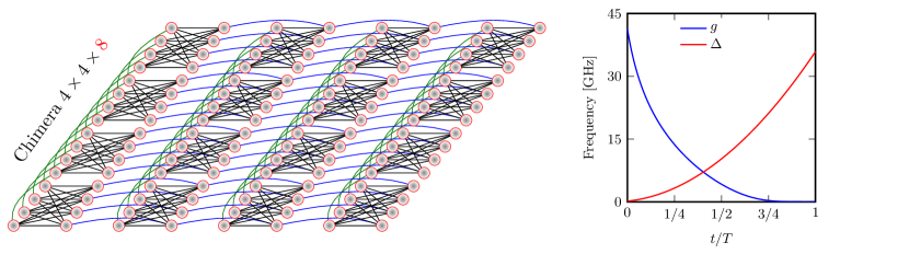
Figure 1: D-Wave processor specification. Left: An example of the Chimera topology, here composed of $4\times 4$ ($C_{4}$) grid consisting of clusters (units cells) of $8$ qubits each. The total number of variables (vertices) for this graph is $N=4\cdot 4\cdot 8=128$. A graph’s edges indicate possible interactions between qubits. The maximum number of qubits is $N_{\text{max}}=2048$ for the Chimera $C_{16}$ topology, whereas the total number of connections between them is limited to $6000\ll N_{\text{max}}^{2}$. Right: A typical annealing schedule controlling the evolution of a quantum processor, where $T$ denotes the time to complete one annealing cycle (the annealing time). It ranges from microseconds ($\sim{}2\mu$s) to milliseconds ($\sim{}2000\mu$s). The parameters $g$ and $\Delta$ are used in (9).

The Ising model, introduced originally for the microscopic explanation of magnetism, has been in the center of the research interests of physicists ever since. It deals with a set of variables $s_{i}\in\{+1,-1\}$ (originally corresponding to the direction of microscopic magnetic momenta associated with spins). The configuration of $N$ such variables is thus described by a vector $\mathbf{s}\in\{+1,-1\}^{N}$. The model then assigns an energy to a particular configuration:

$$E(\mathbf{s})=\sum_{(i,j)\in E}J_{i,j}s_{i}s_{j}+\sum_{i\in V}h_{i}s_{i},$$ (1)

where $(V,E)$ is a graph whose vertices $V$ represent the spins, the edges $E$ define which spins interact, $J_{i,j}$ is the strength of this interaction, and $h_{i}$ is an external magnetic field at spin $i$. Although the early studies of the model dealt with configurations in which the spins were arranged in a one-dimensional chain so that the coupling $J$ was non-zero for nearest neighbors only, the model has-been generalized in many ways, including the most general setting of an arbitrary $(V,E)$ graph, i.e., incorporating the possibly of non-zero couplings for any $i,j$ pair. Such a system is referred to as a spin glass in physics, and it is a physical model that is interesting from an operations research point of view, for the system it describes is a computational resource for optimization. The idea originated from the fact that in physics, the minimum energy configuration determines many properties of a material; hence, a lot of effort has been put into finding it. In addition, the minimum energy configuration can be realized in actual physical systems; thus special hardware – so-called (quantum) annealers – can also be constructed.

In mathematical programming, it is often more convenient to deal with $0$-$1$ variables. By introducing new decision variables ${\mathbf{x}}\in\{0,1\}$ so that

$$x_{i}=\frac{s_{i}+1}{2}$$ (2)

and the matrix

$$Q_{i,i} = 2\left(h_{i}-\sum_{j=1}^{n}J_{i,j}\right)$$

$$Q_{i,j} = 4J_{i,j},$$ (3)

the minimization of the energy function is equivalent to solving a QUBO problem:

$$\begin{array}[]{l@{}ll}\text{min.}&&y=\mathbf{x}^{T}Q\mathbf{x},\\ \text{s.t.}&&\mathbf{x}\in\{0,1\}^{N}.\end{array}$$ (6)

Therefore, minimizing the Ising objective in (1) is equivalent to solving a QUBO. Moreover, the matrix $Q$ can always be chosen to be symmetric, as $Q=(Q^{\prime}+Q^{\prime T})/2$ defines the same objective. Solvers based on Ising spin glasses are actual devices (or specialized algorithms simulating them or calculating their relevant properties) that can handle models of this form only. The technology offers the possibility of efficiently tackling computationally hard problems (when formulated as a QUBO, which is possible for all linear or quadratic $0$-$1$ programs [31]). It does have limitations with respect to size and accuracy, as will be illustrated in the present case study, but it is likely that the technology will continue to improve.

Simultaneously, with the rapid development of quantum annealing technology, probabilistic classical accelerators have been under massive development. In recent years, we have witnessed significant progress in the field of programmable gate array optimization solvers (digital annealers [32]), optical Ising simulators [33], coherent Ising machines [34], stochastic cellular automata [35], and, in general, those based on memristor electronics [36].

It is therefore vital to develop modeling strategies to make operational problems suitable for such models and to create novel techniques to for analyzing the obtained results. This should progress similarly to how powerful solvers for linear programs first started appearing: modeling strategies for linear programs as well as sensitivity analysis were developed ahead of the creation of the hardware.

2.2.2 Quantum annealing

An essential step in finding the minimum of an optimization problem [encoded in (1)] efficiently is to map it to its quantum version. The mapping assigns a two-dimensional complex vector space to each spin, and a complete spin configuration becomes an element of the direct (tensor) products of these spaces. An orthonormal basis (ONB) is assigned to the $-1$ and $+1$ values of the variables; thus the product of these vectors will be an ONB (called the “computational basis”) in the whole $\mathbb{C}^{2^{N}}$. The vectors with unit Euclidean norms are referred to as “states” of the system; they encode the physical configurations. The fact that the state can be an arbitrary vector, and not only an element of the computational basis means that the quantum annealer can simultaneously process multiple configurations, i.e., inherent parallelism.

As to the objective function, the spin variables are replaced by their quantum counterpart: Hermitian matrices acting on the given spin’s $\mathbb{C}^{2}$ tensor subspace:

$$s_{i}\mapsto\hat{\sigma}_{i}^{z}=\mathop{\mbox{diag}}(1,-1),$$ (7)

where the matrix represents the respective operator in the computational basis. The product of spins is meant to be the direct (tensor) product of the respective operators. Thus the objective function (1) turns into a Hermitian operator, referred to as the problem’s Hamiltonian:

$$\mathcal{H}_{\text{p}}:=E(\hat{\bf\sigma}^{z})=\sum_{\langle i,j\rangle\in\mathcal{E}}J_{ij}\hat{\sigma}_{i}^{z}\hat{\sigma}_{j}^{z}+\sum_{i\in\mathcal{V}}h_{i}\hat{\sigma}_{i}^{z},$$ (8)

whose lowest-energy eigenstate is commonly called the “ground state.” In the present case, it is an element of the computational basis, so it represents also the optimal configuration of the classical problem. Note that the energy of a physical system is related (via eigenvalues) to a Hermitian operator, called its Hamiltonian. Although it seems to be a significant complication to deal with $\mathbb{C}^{2^{N}}$ instead of having $2^{N}$ binary vectors, it has important benefits, the most remarkable of which is that they model realistic physical systems, so they are realized by nature.

The main idea behind quantum annealing is based on the celebrated adiabatic theorem [37]. Broadly speaking, when a quantum system (starting from its ground state) is driven (i.e., its Hamiltonian is adjusted in time) slowly enough that it has time to adjust to changes, it can remain in its ground state during the entire evolution. At the end of the systems evolution, a solution to a computational problem can be read out from the final state.

To be more specific, assume that a quantum system can be prepared in the ground state of an initial (“simple”) Hamiltonian $\mathcal{H}_{0}$. Then it will slowly evolve to the ground state of the final (“complex”) Hamiltonian $\mathcal{H}_{\text{p}}$ in (8) that can be harnessed to encode the solution of an optimization problem [30]. In particular, the dynamics of the current D-Wave $2000$Q quantum annealer is governed by the following time-dependent Hamiltonian [4, 38]:

$$\mathcal{H}(t)/(2\pi\hbar)=-g(t)\mathcal{H}_{0}-\Delta(t)\mathcal{H}_{\text{p}^{\prime}},\quad t\in[0,T].$$ (9)

Here the original problem’s Hamiltonian in (8) must be converted into a bigger one $\mathcal{H}_{\text{p}^{\prime}}$ whose graph is compliant with the existing hardware can realize: the “Chimera graph” (see Fig. 1). The original problem’s graph will be the minor of this graph. This procedure, called “minor embedding”, is standard in quantum annealing procedures (see also Section 4.3 for a simple graphical representation of this Chimera embedding).

In fact, many relevant optimization problems are defined on dense graphs. Fortunately, even complete graphs can be embedded into a Chimera graph [39]. There is, however, substantial overhead, which effectively limits the size of the computational graph that can be treated with current quantum annealers [40, 41]. This is, nevertheless, believed to be an engineering issue that will most likely be overcome in the near future [1, 42]. After the Chimera embedding, the Hamiltonian describing the system reads as follow:

$$\mathcal{H}_{\text{p}^{\prime}}=\sum_{\langle i,j\rangle\in\mathcal{E}}J^{\prime}_{ij}\hat{\sigma}_{i}^{z}\hat{\sigma}_{j}^{z}+\sum_{i\in\mathcal{V}}h^{\prime}_{i}\hat{\sigma}_{i}^{z}\quad\text{and}\quad\mathcal{H}_{0}=\sum_{i}\hat{\sigma}_{i}^{x},$$ (10)

where

$$\sigma^{X}=\begin{bmatrix}0&1\cr 1&0\end{bmatrix}$$ (11)

in the computational basis and $\hat{\sigma}^{Z}$ is defined in (7). The annealing time $T$ varies from microseconds ($\sim{}2\mu$s) to milliseconds ($\sim{}2000\mu$s) depending on the specific programmable schedule [4]. As shown in Fig. 1, during the evolution, $g(T)$ varies from $g(0)\gg 0$ (i.e., all spins point in the $x$-direction) to $g(T)\approx 0$, whereas $\Delta(t)$ is changed from $\Delta(0)\approx 0$ to $\Delta(T)\gg 0$ (i.e., $\mathcal{H}(T)\sim\mathcal{H}_{\text{p}^{\prime}}$). The Pauli operators $\hat{\sigma}_{i}^{z}$, $\hat{\sigma}_{i}^{x}$ describe the spin’s degrees of freedom in the $z$- and $x$-direction, respectively. Note that the Hamiltonian $\mathcal{H}_{\text{p}}$ is classical in the sense that all its terms commute (which is the result of their multiplication being independent of the order). Thus, as mentioned previously, its eigenstates translate directly to classical variables, $q_{i}=\pm 1$, which are introduced to encode discrete optimization problems.

The annealing time, $T$ in (9), is an important parameter of the quantum annealing process: it must be chosen so that the system reaches its ground state while the adiabaticity is at least approximately maintained. The adiabatic theorem gives us a guidance in this respect. In the spectrum of the Hamiltonian in (9), there is a difference between the energy of the ground state(s) and the energy of the state(s) just above it in energy scale. This difference is known as the (spectral) “gap”, and its minimum value in the course of the evolution determines the required computation time if certain additional conditions hold. Roughly speaking, the bigger the gap, the faster the quantum system reaches its ground state (the dependence is actually quadratic; see Ref. [43] for a detailed discussion). Thus, if the run time is not optimal, there is a finite probability of reading out an excited state instead of the true ground state. Therefore, the ideal approach would be to calculate the optimal time, and only then let the system evolve for as long as it is necessary. However, the spectrum is actually unknown, and its determination is at least as hard as solving the optimization problem itself. Hence, in practice, a reasonable annealing time is educatedly guessed, and the evolution is repeated reasonably many times, resulting in a sample of possible solutions (over different annealing times as well as other relevant parameters). The one with the lowest energy is considered to be the desired solution, albeit there is a finite probability that it is not the ground state. A quantum annealer is thus a probabilistic and heuristic solver. Concerning the benchmarking of quantum annealers, consult also [44].

As a side note, it should be stressed that it is not always possible to maintain the adiabatic evolution. As an example, consider the second–order phase transition phenomenon [45, 46, 47], in which even a short–lasting lack of adiabaticity will result in the creation of topological defects preventing the system from remaining in its instantaneous ground state. This effect, on the other hand, is a clear manifestation of the Kibble–Żurek mechanism [48, 49, 50] and can be used to detect departures from adiabaticity.

2.2.3 Classical algorithms for solving Ising problems

An additional benefit of formulating problems in terms of Ising-type models is that the existing methods developed in statistical and solid-state physics for finding ground states of physical systems can also be used to solve a QUBO on classical hardware. Notably, variational methods based on finitely correlated states (such as matrix product states for 1D systems or projected entangled pair states suitable for 2D graphs) have had a very extensive development in the past few decades. A quantum information theoretic insight into density matrix renormalization group methods (DMRG [51]) – being the most powerful numerical techniques in solid-state physics at that time – helped in proving the correctness of DMRG. These methods also led to a more general view of the problem [52], resulting in many algorithms that have potential applications in various problems, in particular solving QUBOs by finding the ground state of a quantum spin glass. We have used the algorithms presented in [53] to solve the models derived in the present manuscript.

Both quantum computers and the mentioned classical algorithms may not provide the energy minimum and the corresponding ground state (as it is not trivial to reach it [54]) but another eigenstate of the problem with an eigenvalue (i.e., a value of the objective function) close to the minimum. The corresponding states are referred to as “excited states.” Another important point in interpreting the results of such a solver is the degeneracy of the solution: the possibility of having multiple equivalent optima.

In analyzing these optima, it is helpful that for up to 50 variables, one can calculate the exact ground states and the excited states closest to them using a brute-force search on the spin configurations with GPU-based high-performance computers. In the present work, we also use such algorithms, in particular those introduced in [3] for benchmarking and evaluating our results for smaller examples. This way we can compare the exact spectrum with the results obtained from the D-Wave quantum hardware and the variational algorithms.

2.3 Quantum computing for railway optimization

Quantum computing is an emerging technology that is still in its infancy. So far, at least in public domain research, most of the problems addressed are not directly related to a particular industrial application but concern the solution of “classical” generic hard computational problems, such as, e.g. the traveling salesman problem or the graph coloring problem; some of these are listed in [55]. Meanwhile there is a growing interest in quantum optimization techniques as they are becoming increasingly available, both in the confidential industrial and the public research domain.

In the domain of transportation research, the applicability of quantum annealing has until now been demonstrated only in a few areas; the contribution closest to ours is in the field of air traffic management. Stollenwerk et al. [56] have recently addressed a class of simplified air traffic management problems of strategic conflict resolution. (Yet this is still a dispatching problem of a very different nature, resulting from the specifics of air and rail traffic.) Their preliminary results show that some of the challenging problems can be solved efficiently with the D-Wave $2000$Q machine.

As to the railway industry, to the best of our knowledge, the present work is the first one to apply a quantum computing approach to a problem in railway optimization. Even though there are some quantum-inspired methods (such as the one described in [57] for rolling stock rostering), they do not use quantum computers but borrow certain ideas from the mathematics of quantum mechanics. Although our problem shows certain similarities in QUBO formulation to that in [56], it is definitely a different case that we handle with another approach. To demonstrate this difference more clearly, observe that in the approach of [56] there are far fewer potential conflicting situations per vehicle than in ours (see Tables $1$ and $2$ in [56], in which there are approximately $2$ potential conflicting situations per flight in most cases). This leads to different sizes and specifics when the optimization problem is transformed to QUBO.

3 Our model

In this section, we introduce the model of the railway line and the dispatching conditions. Table 1 provides a comprehensive summary of the notation used.

symbol	description / explanation
$A_{j,s}$	discretized set of all possible delays of train $j$ at station $s$
$\mathcal{H}(t)$, $\mathcal{H}_{0}$, $\mathcal{H}_{p}$	time-dependent Hamiltonian of the annealing process and its time-independent components
$t\in[0,T]$	quantum annealing time
$\hat{\sigma}^{x},\hat{\sigma}^{z}$	Pauli matrices
$j\in\mathcal{J}$	trains (jobs)
$\mathcal{J}^{0}$ ($\mathcal{J}^{1}$)	trains heading in a given (opposite) direction
$m\in\mathcal{M}$	blocks (machines)
$s\in\mathcal{S}$	station blocks
$l\in\mathcal{L}$	line blocks
$M_{j},(S_{j})$	the sequence of blocks (station blocks) in the route of $j$
$s_{j,1},s_{j,k},s_{j,\text{end}}$	the first, $k$-th, and last station block in the route of $j$
$m_{j,1},m_{j,k},m_{j,\text{end}}$	the first, $k$-th, and last block in the route of $j$
$S_{j}=(s_{j,1},s_{j,2},\ldots,s_{j,\text{end}})$	a sequence of all station blocks in $j$’s route
$S_{j}^{*}$, ($S_{j}^{**}$)	a sequence of station blocks in $j$’s route without the last (last two) elements
$S_{j,j^{\prime}}$	a common path of $j$ and $j^{\prime}$, ordered according to $j$’s path
$S^{*}_{j,j^{\prime}}$	a common path of $j$ and $j^{\prime}$ excluding the last block, ordered according to $j$’s path
$\rho_{j}(m),\rho_{j}(s)$	the subsequent block (station block) in $j$’s route
$\pi_{j}(m),\pi_{j}(s)$	the preceding block (station block) in $j$ ’s route
$t_{\text{out}}(j,s)$, ($t_{\text{in}}(j,s)$)	time of leaving (entering) station block $s$ by train $j$
$t^{\text{timetable}}_{\text{out}}(j,s)$	timetable time of leaving $s$ by $j$
$p_{\text{timetable}}(j,m)$, $p_{\text{min}}(j,m)$	timetable and minimum time of $j$ passing $m$
$d(j,s)$	delay of $j$ leaving $s$
$d_{U}(j,s)$	primary (unavoidable) delay of $j$ leaving $s$
$d_{s}(j,s)$	secondary delay of $j$ leaving $s$
$d_{\text{max}}(j)$	maximum possible (acceptable) secondary delay for train $j$
$\tau_{(1)}(j,...)\tau_{(2)}(j,...)$	minimum time for train $j$ to give way to another train going in the same (opposite) direction
$x,(\mathbf{x}$)	binary decision variable (vector of binary decision variables), e.g., $x_{j,s,d}=x_{i}$ is $1$ if $j$ leaves $s$ with a delay $d$ and $0$ otherwise, $i\in\{1,2,\ldots,n\}$
$Q\in{\mathbb{R}}^{n\times n}$	symmetric QUBO matrix, where $n$ is the number of logical quantum bits.
$f(\mathbf{x})$	objective function; the weighted sum of secondary delays

Table 1: Summary of notations used

3.1 Railway line

We assume a railway line $\mathcal{M}$ to be a set of block sections (see Section 2.1.1). These are either line blocks or station blocks; both are also refereed to as block sections or just blocks. The set of line blocks are denoted by $\mathcal{L}$, and the set of station blocks by $\mathcal{S}$. This model also incorporates sidings or double-track sections by treating them as station blocks.

Trains can only meet and pass (M-P) or meet and overtake (M-O) at stations. We follow the buffer approach by treating each station as a block that can be occupied by up to $b$ trains at a time, where $b$ is the number of tracks at the station. The other blocks can be occupied by only one train at a time.

The set of trains is denoted by $\mathcal{J}$ and is split into the subset of trains traveling in a given direction $\mathcal{J}^{0}$ and the subset of trains going in the opposite direction $\mathcal{J}^{1}$:

$$\mathcal{J}^{0}\cup\mathcal{J}^{1}=\mathcal{J}\text{ and }\mathcal{J}^{0}\cap\mathcal{J}^{1}=\emptyset.$$ (12)

Let $j\in\mathcal{J}$ be a particular train. Its route is a sequence of blocks $M_{j}=(m_{j,1},m_{j,2},\ldots,m_{j,\text{end}})$, where $m_{j,1}$ is the starting block and $m_{j,\text{end}}$ is the ending block. Each block (from $M_{j}$) is passed by train $j$ once and only once (i.e., we do not consider recirculation). Given a train $j$ and a block $m_{j,k}$, the preceding block is $\pi_{j}(m_{j,k})=m_{j,k-1}$, while the subsequent block is $\rho_{j}(m_{j,k})=m_{j,k+1}$. We assume that neither $\rho_{j}(m_{j,\text{end}})$ nor $\pi_{j}(m_{j,1})$ belongs to the analyzed network segment.

We assume that a route can be defined solely by a sequence of station blocks $S_{j}=(s_{j,1},s_{j,2},\ldots,s_{j,\text{end}})$, where M-P and M-O may occur (i.e., there are no alternative routes between stations). Similarly to blocks in general, for a train $j$ and a station block $s_{j,k}$, we denote the preceding station block as $\pi_{j}(s_{j,k})=s_{j,k-1}$, and the subsequent station block as $\rho_{j}(s_{j,k})=s_{j,k+1}$. It is convenient to assume that all train paths start and end at stations; hence we have $s_{j,1}=m_{j,1}$ and $s_{j,\text{end}}=m_{j,\text{end}}$.

3.2 Delay representation

Ideally, the time $t_{\text{out}}(j,s)$ when train $j$ leaves station block $s$ should be the time prescribed by the timetable, $t^{\text{timetable}}_{\text{out}}(j,s)$. If, however, $t_{\text{out}}(j,s)>t^{\text{timetable}}_{\text{out}}(j,s)$, there is a delay in leaving station block $s$:

$$d(j,s)=t_{\text{out}}(j,s)-t^{\text{timetable}}_{\text{out}}(j,s).$$ (13)

Primary or unavoidable delays (as defined in Section 2.1.1) are denoted by $d_{U}(j,s)$. If an already delayed train enters a railway line $\mathcal{M}$, the initial delay will appear at the first block $d_{U}(j,s_{j,1})$. The unavoidable delay propagates along the line, thereby providing a lower bound of the overall delay. Unavoidable delays are non-negative, so we have

$$d_{U}(j,\rho_{j}(s))=\max\{d_{U}(j,s)-\alpha(j,s,\rho_{j}(s)),0\},$$ (14)

where $\alpha(j,s,\rho_{j}(s))$ accounts for the possible time reserve in passing the sequence of blocks, starting from the one directly after $s$ and ending at station block $\rho_{j}(s)$. In the same way, the unavoidable delays are propagated due to the minimum times of the rolling stock circulation at terminals. Importantly, all unavoidable delays can be computed prior to the optimization.

The secondary delay $d_{S}(j,s)$ is denoted by

$$d_{S}(j,s)=d(j,s)-d_{U}(j,s).$$ (15)

We introduce upper bounds $d_{\text{max}}(j)$ of the secondary delays as parameters of the model. Their values can either be determined manually (maximum acceptable secondary delays of the given trains) or be obtained by using some fast heuristics such as the first come first served (FCFS) or first leave first served (FLFS) approach (which will be discussed later). Setting them too low, however, can result in an unfeasible model.

Having established the upper and lower bounds,

$$d_{U}(j,s)\leq d(j,s)\leq d_{U}(j,s)+d_{\text{max}}(j),$$ (16)

we can use the (integer) values of the delays as decision variables. The bounds ensure that these variables remains in a finite range. In what follows, we shall call this description, in terms of the discretized delays as decision variables, “delay representation”; it will be very convenient from the QUBO modeling point of view.

3.3 Dispatching conditions

Consider a train $j$ whose path $M_{j}$ consists of both station and line blocks. We assume that the leaving time of the given block equals the entering time of the subsequent block:

$$t_{\text{out}}(j,m)=t_{\text{in}}(j,\rho_{j}(m)).$$ (17)

(This is a slight simplification as there is a finite time in which the train is located in both blocks.) For each train $j\in\mathcal{J}$ and each block $m\in M_{j}$, two kinds of passing times are assigned: a nominal (timetable) $p_{\text{timetable}}(j,m)$ and a minimum $p_{\text{min}}(j,m)$. Note that the latter can be smaller or equal to $p_{\text{timetable}}(j,m)$ (as there can be a reserve).

We address common dispatching conditions, including: the minimum passing time condition, the single block occupation condition, the deadlock condition, the rolling stock circulation condition at the terminal, and the capacity condition.

Condition 3.1.

The minimum passing time condition. The leaving time from the block section cannot be lower than the sum of the entering time and the minimum passing time:

$$t_{\text{out}}(j,m)\geq t_{\text{in}}(j,m)+p_{\text{min}}(j,m).$$ (18)

For subsequent station blocks $s=m_{j,k}$ and $\rho_{j}(s)=m_{j,l}$, we have

$$t_{\text{out}}(j,\rho_{j}(s))\geq t_{\text{out}}(j,s)+\sum_{i=k+1}^{l}p_{\text{min}}(j,m_{j,i})=t_{\text{out}}(j,s)+\sum_{i=k+1}^{l}p_{\text{timetable}}(j,m_{i})-\alpha(j,s,\rho_{j}(s)),$$ (19)

where $\alpha(j,s,\rho_{j}(s))$ is the time reserve mentioned before. In the delay representation, this condition takes the simple form

$$d(j,\rho_{j}(s))\geq d(j,s)-\alpha(j,s,\rho_{j}(s)).$$ (20)

(Compare this with (14), where we have an equal sign for the lower limit.)

Condition 3.2.

The single block occupation condition. Let $j$ and $j^{\prime}$ be two trains heading in the same direction and sharing their routes between station $s$ and subsequent station $\rho_{j}(s)$. If train $j$ leaves station block $s$ at time $t_{\text{out}}(j,s)$, the subsequent ($t_{\text{out}}(j^{\prime},s)\geq t_{\text{out}}(j,s)$) train $j^{\prime}$ can leave this block at a time for which the following equation is fulfilled:

$$t_{\text{out}}(j^{\prime},s)\geq t_{\text{out}}(j,s)+\tau_{(1)}(j,s,\rho_{j}(s)),$$ (21)

where $\tau_{(1)}(j,s,\rho_{j}(s))$ is the time required for train $j$ to give way to train $j^{\prime}$ on the route between station block $s$ and subsequent station block $\rho_{j}(s)$. In the delay representation we have:

$$d(j^{\prime},s)+t^{\text{timetable}}_{\text{out}}(j^{\prime},s)\geq d(j,s)+t^{\text{timetable}}_{\text{out}}(j,s)+\tau_{(1)}(j,s,\rho_{j}(s))$$ (22)

or

$$d(j^{\prime},s)\geq d(j,s)+t^{\text{timetable}}_{\text{out}}(j,s)-t^{\text{timetable}}_{\text{out}}(j^{\prime},s)+\tau_{(1)}(j,s,\rho_{j}(s)).$$ (23)

Hence, taking $\Delta(j,s,j^{\prime},s)=t^{\text{timetable}}_{\text{out}}(j,s)-t^{\text{timetable}}_{\text{out}}(j^{\prime},s)$, we get

$$d(j^{\prime},s)\geq d(j,s)+\Delta(j,s,j^{\prime},s)+\tau_{(1)}(j,s,\rho_{j}(s)).$$ (24)

As mentioned before, the condition in (24) needs to be tested for $t_{\text{out}}(j^{\prime},s)\geq t_{\text{out}}(j,s)$, i.e., $d(j^{\prime},s)\geq d(j,s)+\Delta(j,s,j^{\prime},s)$; otherwise trains must be investigated in the reversed order.

The actual form of $\tau_{(1)}(j,s,\rho_{j}(s))$ depends on the dispatching details of the particular problem. We assume that all the time reserves are realized on stations. Consequently, $\tau_{(1)}(j,s,\rho_{j}(s))$ is delay independent, which makes the problem tractable.

Condition 3.3.

The deadlock condition. Assume that two trains $j$ and $j^{\prime}$ are heading in opposite directions on a route determined by subsequent station blocks $s$ and $\rho_{j}(s)$ in the path of train $j$. In the path of $j^{\prime}$, these are reversed, so $j$ goes $s\rightarrow\rho_{j}(s)$, while $j^{\prime}$ goes $\rho_{j}(s)\rightarrow s$. Assume for now that the train $j$ will enter the common block section before $j^{\prime}$. (This condition must also be checked in the reverse order.) Let $\tau_{(2)}(j,s,\rho_{j}(s))$ be the time required for the train $j$ to get from station block $s$ to $\rho_{j}(s)$. Given this, the deadlock condition can be stated as follows:

$$t_{\text{out}}(j^{\prime},\rho_{j}(s))\geq t_{\text{in}}(j,\rho_{j}(s)),$$ (25)

i.e.,

$$t_{\text{out}}(j^{\prime},\rho_{j}(s))\geq t_{\text{out}}(j,s)+\tau_{(2)}(j,s,\rho_{j}(s)).$$ (26)

In the delay representation,

$$d(j^{\prime},\rho_{j}(s))+t^{\text{timetable}}_{\text{out}}(j^{\prime},\rho_{j}(s))\geq d(j,s)+t^{\text{timetable}}_{\text{out}}(j,s)+\tau_{(2)}(j,s,\rho_{j}(s))$$ (27)

and

$$d(j^{\prime},\rho_{j}(s))\geq d(j,s)+t^{\text{timetable}}_{\text{out}}(j,s)-t^{\text{timetable}}_{\text{out}}(j^{\prime},\rho_{j}(s))+\tau_{(2)}(j,s,\rho_{j}(s)).$$ (28)

Hence, taking $\Delta(j,s,j^{\prime},\rho_{j}(s))=t^{\text{timetable}}_{\text{out}}(j,s)-t^{\text{timetable}}_{\text{out}}(j^{\prime},\rho_{j}(s))$, we get:

$$d(j^{\prime},\rho_{j}(s))\geq d(j,s)+\Delta(j,s,j^{\prime},\rho_{j}(s))+\tau_{(2)}(j,s,\rho_{j}(s)).$$ (29)

Again, condition (29) needs to be tested for $t_{\text{out}}(j^{\prime},\rho_{j}(s))\geq t_{\text{out}}(j,s)$; otherwise trains must be investigated in the reversed order.

Further, similarly to Condition 3.2, the form of $\tau_{(2)}(j,s,\rho_{j}(s))$ depends on the dispatching details resulting from the formulation of the problem. Again, as all time reserves are assumed to be realized at stations, $\tau_{(2)}(j,s,\rho_{j}(s))$ is delay independent, which makes the problem more tractable.

As mentioned before, the particular form of the $\tau$s are problem dependent; we propose the following approach to this. Suppose that train $j$ departs from station $s$ to subsequent station $\rho_{j}(s)$, passing the blocks $m_{k},m_{k+1},\ldots,m_{l-1},m_{l}$, where $s=m_{k}$ and $m_{l}=\rho_{j}(s)$. The subsequent train proceeding in the same direction is allowed to leave at least after

$$\tau_{(1)}\left(j,s\right)=\max_{i\in\{k+1,\ldots,l-1\}}\left(t_{\text{in}}^{\text{timetable}}(j,m_{i+1})-t_{\text{in}}^{\text{timetable}}(j,m_{i})\right).$$ (30)

The subsequent train proceeding in the opposite direction is allowed to leave at least after

$$\tau_{(2)}\left(j,s\right)=\sum_{i\in\{k+1,\ldots,l-1\}}\left(t_{\text{in}}^{\text{timetable}}(j,m_{i+1})-t_{\text{in}}^{\text{timetable}}(j,m_{i})\right)\equiv t_{\text{in}}^{\text{timetable}}(j,\rho_{j}(s))-t_{\text{out}}^{\text{timetable}}(j,s).$$ (31)

Referring to the minimum and maximum delay conditions – see (16) – there are pairs of trains for which either Condition 3.2, or Condition 3.3, is always fulfilled. This observation simplifies our QUBO representation of the problem.

Condition 3.4.

Rolling stock circulation condition at the terminal. If train $j$ with a given train set assigned terminates at a station where the next train $j^{\prime}$ of the same train set starts its course (after turnover), i.e., $s_{j,end}=s_{1,j^{\prime}}$, the following condition arises:

$$t_{\text{out}}(j^{\prime},s_{j^{\prime},1})>t_{\text{in}}(j,s_{j,end})+\Delta(j,j^{\prime}),$$ (32)

where $\Delta(j,j^{\prime})$ is the minimum turnover time. In the delay representation, we have

$$d(j^{\prime},1)+t^{\text{timetable}}_{\text{out}}(j^{\prime},1)>d(j,s_{j,end-1})+t^{\text{timetable}}_{\text{out}}(j,s_{j,end-1})+\tau_{(2)}\left(j,s_{j,end-1})\right)+\Delta(j,j^{\prime}).$$ (33)

Hence, taking $R(j,j^{\prime})=t^{\text{timetable}}_{\text{out}}(j^{\prime},1)-t^{\text{timetable}}_{\text{out}}(j,s_{j,end-1})-\tau_{(2)}\left(j,s_{j,end-1})\right)-\Delta(j,j^{\prime})$, we get

$$d(j^{\prime},1)>d(j,s_{j,end-1})-R(j,j^{\prime}).$$ (34)

Condition 3.5.

The capacity condition. Here we include the buffer approach of handling stations in our model. Suppose we have a station block $s$, capable of handling up to $b$ trains at a time. Let $\{j_{1},j_{2},\ldots,j_{b+1}\}\subset\mathcal{J}$ be any $b+1$-tuple of trains. No time $t$ may exist for which all the conditions below are simultaneously fulfilled:

$$t_{\text{in}}(j_{1},s) \leq t\leq t_{\text{out}}(j_{1},s)$$

$$\ldots$$

$$t_{\text{in}}(j_{b+1},s) \leq t\leq t_{\text{out}}(j_{b+1},s).$$ (35)

In the delay representation,

$$d(j_{1},\pi_{j_{1}}(s))+t^{\text{timetable}}_{\text{out}}(j_{1},\pi_{j_{1}}(s))+\tau_{(2)}\left(j_{1},\pi_{j}(s)\right) \leq t\leq d(j_{1},s)+t^{\text{timetable}}_{\text{out}}(j_{1},s)$$

$$\ldots$$

$$d(j_{b+1},\pi_{j_{1}}(s))+t^{\text{timetable}}_{\text{out}}(j_{b+1},\pi_{j_{b+1}}(s))+\tau_{(2)}\left(j_{b+1},\pi_{j}(s)\right) \leq t\leq d(j_{b+1},s)+t^{\text{timetable}}_{\text{out}}(j_{b+1},s).$$ (36)

As a consequence of Condition 3.5, many new constraints may arise. These may make the calculations more complex, even exceeding the capacity of the current quantum computers. In our particular problem instances, we will temporarily ignore this condition, but we will verify the solutions against it.

Finally, it is worth observing that Conditions 3.1 - 3.5 refer to station blocks only; line blocks do not appear. As we have a single-track line, there is no need to analyze line blocks in the optimization algorithm: the decisions are made at the stations. The leaving time from the ending (station) block does not have to be analyzed either.

3.4 Linear integer programming approach

Before proceeding to the QUBO approach we describe a linear integer programming formulation, too. This is in the line with the standard treatment of railway dispatching problems; meanwhile, it is formulated so that it is compares easily with the QUBO approach. It will therefore be used as a reference for comparisons.

Similarly to the model in [18], we opt for using precedence variables as it is very suitable for a single-track railway model. We introduce the binary decision variables $y_{j,j^{\prime},k}$ so that they have a value of $1$ if the train $j$ occupies the particular part of the track (denoted by $k$) before train $j^{\prime}$, and are zero otherwise.

Train delays will be represented with discrete decision variables $d(j,s)$ that fulfil (16). (The discretization is not necessary, but it is practical for the comparison with the QUBO results, as the discretization is required there and our particular problem instances were found to be tractable with a standard solver.)

Note that the ordering of the train departures is uniquely described by the precedence variables ($y$s), but for each configuration there is still some freedom in determining the value of the delay variables ($d$s). For the solution to be valid, the values of the $y$s and $d$s should be consistent; this will be ensured by the constraints.

The constraints are the following. The constraints in (20), and (34) are linear; hence, they can directly be included in the model. The single block occupation condition, see (24), is expressed in terms of the precedence and delay variables:

$$d(j^{\prime},s)+M\cdot(1-y_{j,j^{\prime},s})\geq d(j,s)+\Delta(j,s,j^{\prime}s)+\tau_{(1)}(j,s,\rho_{j}(s)),$$ (37)

where $y_{j,j^{\prime},s}$ determines the order of trains $j$ and $j^{\prime}$ leaving station $s$, and $M$ is an arbitrary large number. For two trains $j$ and $j^{\prime}$ heading in opposite directions, the deadlock condition is to be prescribed. For trains with a common path between subsequent stations $k\rightarrow\{s,\rho_{j}(s)\}$, the requirement in (29) takes the following form:

$$d(j^{\prime},s)+M\cdot(1-y_{j,j^{\prime},k})\geq d(j,s)+\Delta(j,s,j^{\prime}\rho_{j}(s))+\tau_{(2)}(j,s,\rho_{j}(s)),$$ (38)

where $y_{j,j^{\prime},k}$ determines which train enters the common path first.

Finally, as to the objective function, the weighted sum of secondary delays (or the total weighted tardiness in the scheduling terminology) will be minimized, which is also inherently linear:

$$\min\sum_{j}\frac{d(j,s_{j,\text{end}-1})-d_{U}(j,s_{j,\text{end}-1})}{d_{\text{max}}(j)}w_{j},$$ (39)

where $w_{j}$ is the weight reflecting the train’s priority.

Although the defined linear model is suitable for the given railway environment, our intention is to use a solver that inputs QUBOs. For this purpose, an integer program is not a good choice; hence, we construct an alternative quadratic model with binary decision variables.

4 QUBO formulation of our model

We construct a QUBO model that can be solved either by quantum annealers or by classical algorithms inspired by them. After presenting a constrained $0$-$1$ representation, we employ a penalty method to move the constraints to the effective objective function to get an unconstrained problem. This is maybe the most challenging step, not only in our present work, but also in logical programming using QUBOs.

4.1 0-1 program representation

As a step toward a QUBO model, we formulate our problem entirely in terms of binary decision variables. We achieve this by the discretization of time, i.e., the discretization of the delay variables. Hence, we need to set a delay resolution step. We opt for a resolution of one minute as this is reasonable from train timetabling point of view (and the generalization is straightforward). Given such a representation, (16) can be rewritten into the following form:

$$d(j,s)\in A_{j,s}=\{d_{U}(j,s),d_{U}(j,s)+1,\ldots,d_{U}(j,s)+d_{\text{max}}(j)\},$$ (40)

where $A_{j,s}$ is a discretized set of all possible delays of train $j$ at station $s$.

For the QUBO representation, we introduce the binary decision variables

$$x_{s,j,d}\in\{0,1\},$$ (41)

which take the value of $1$ if train $j$ leaves station block $s$ at delay $d$, and zero otherwise. These variables will also be referred to as “QUBO variables.” Their vector is $\mathbf{x}\in\{0,1\}^{n}$. Each variable is assigned a logical quantum bit. Hence solving the problem requires $n$ of these bits. The number $n$ depends on the size of the system and is dependent on the number of trains and stations and the value of the maximum secondary delay.

We assume that each train leaves each station block once and only once:

$$\forall_{j}\forall_{s\in S_{j}}\sum_{d\in A_{j,s}}x_{s,j,d}=1.$$ (42)

Remark 4.1.

Observe that Conditions 3.2 and 3.3 (the single block occupation condition and the deadlock condition) refer to the subsequent stations in train $j$ path – $s$ and $\rho_{j}(s)$. (Recall that $\rho_{j}(s_{j,\text{end}})$ does not exist in our model.) Time of entering of $\rho_{j}(s)$ is computed from $x_{s,j,d}$ and $\tau_{(1)}(j,s,\rho_{j}(s))$, but it does not refer to $x_{\rho_{j}(s),j,d}$. Hence we do not need to investigate the leaving time from the last block of the train’s path. We assume that the arrival time at this block can be computed from the leaving time from the penultimate block and the passing time. (Of course, our goal is to reduce the number of QUBO variables in the analysis.) Here, delays at the end of the route are investigated on leaving the penultimate station of the analyzed route.

Let $S_{j,j^{\prime}}$ be the sequence of blocks in the common route of trains $j$ and $j^{\prime}$. If both these trains are traveling in the same direction, the order of blocks in $S_{j,j^{\prime}}$ is straightforward. Alternatively, we need to regard the block sequence of train $j$ as the reversed sequence of blocks of train $j^{\prime}$. Therefore, we introduce $S_{j,j^{\prime}}^{*}=S_{j,j^{\prime}}\setminus\{s_{j,\text{end}}\}$ for Conditions 3.2 and 3.3. Condition 3.2 states that two trains traveling in the same direction are not allowed to appear at the same block section. In particular, from (24) it follows that

$$\forall_{(j,j^{\prime})\in\mathcal{J}^{0}(\mathcal{J}^{1})}\forall_{s\in S^{*}_{j,j^{\prime}}}\sum_{d\in A_{j,s}}\left(\sum_{d^{\prime}\in B(d)\cap A_{j^{\prime},s}}x_{j,s,d}x_{j^{\prime},s,d^{\prime}}\right)=0,$$ (43)

where $B(d)=\{d+\Delta(j,s,j^{\prime},s),d+\Delta(j,s,j^{\prime},s)+1,\ldots,d+\Delta(j,s,j^{\prime},s)+\tau_{(1)}(j,s,\rho_{j}(s))-1\}$ is a set of delays that violates Condition 3.2.

Assume now that two trains $j$ and $j^{\prime}$ are heading in opposite directions. From (29) it follows that

$$\forall_{j\in\mathcal{J}^{0}(\mathcal{J}^{1}),j^{\prime}\in\mathcal{J}^{1}(\mathcal{J}^{0})}\forall_{s\in S^{*}_{j,j^{\prime}}}\sum_{d\in A_{j,s}}\left(\sum_{d^{\prime}\in C(d)\cap A_{j^{\prime},\rho_{j}(s)}}x_{j,s,d}x_{j^{\prime},\rho_{j}(s),d^{\prime}}\right)=0$$ (44)

where $C(d)=\{d(j,s)+\Delta(j,s,j^{\prime},\rho_{j}(s)),d(j,s)+\Delta(j,s,j^{\prime},\rho_{j}(s))+1,\ldots,d(j,s)+\Delta(j,s,j^{\prime},\rho_{j}(s))+\tau_{(2)}(j^{\prime},\rho_{j}(s))-1\}$.

We do not need to examine delays when leaving the ending station of the train’s path; see Remark 4.1. For the minimum passing time – Condition 3.1 – we introduce $S_{j}^{**}=S_{j}\setminus\{s_{j,end},s_{j,end-1}\}$. From (20) we have:

$$\forall_{j}\forall_{s\in S_{j}^{**}}\sum_{d\in A_{j,s}}\left(\sum_{d^{\prime}\in D(d)\cap A_{j,\rho_{j}(s)}}x_{j,s,d}x_{j,\rho_{j}(s),d^{\prime}}\right)=0,$$ (45)

where $D(d)=\{0,1,\ldots,d-\alpha(j,s,\rho_{j}(s))-1\}$.

Following the the rolling stock circulation (Condition 3.4) we have, from (34),

$$\forall_{j,j^{\prime}\in\text{terminal pairs}}\sum_{d\in A_{j,s_{(j,end-1)}}}\sum_{d^{\prime}\in E(d)\cap A_{j^{\prime},1}}x_{j,s_{(j,end-1)},d}\cdot x_{j^{\prime},s_{(j,^{\prime}1)},d^{\prime}}=0,$$ (46)

where $E(d)=\{0,1,\ldots,d-R(j,j^{\prime})\}$.

The objective of the algorithm is to schedule trains so that secondary delays are minimized. The general objective function can be written in the following form:

$$f(d,j,s)=\hat{f}\left(\hat{d},j,s\right),$$ (47)

where $\hat{d}=\frac{d(j,s)-d_{U}(j,s)}{d_{\text{max}}(j)}.$ As discussed in Section 2.1.1, primary delays ($d_{U}$) are unavoidable, so they are not relevant for the objective. Recall that upper bounds of the secondary delays $d_{\text{max}}(j)$ have been introduced as parameters, see (16). Thus we require $\hat{f}(\hat{d},j,s)$ to fulfill the following conditions:

$$\hat{f}(\hat{d},j,s)=\begin{cases}0&\text{ if }\hat{d}=0,\\ \max_{\hat{d}\in[0,1]}\hat{f}(\hat{d},j,s)&\text{ if }\hat{d}=1,\\ \text{is non-decreasing in }\hat{d}&\text{ if }\hat{d}\in(0,1).\end{cases}$$ (48)

This non-decreasing property reflects that higher delays cannot contribute to a lower extent to the objective. Finally, our objective function will be linear:

$$f(\mathbf{x})=\sum_{j\in J}\sum_{s\in S_{j}^{*}}\sum_{d\in A_{j,s}}f(d,j,s)\cdot x_{j,s,d},$$ (49)

where $f(d,j,s)$ are the weights.

Apart from the constraints discussed above, the penalty function can be chosen deliberately, which adds some relevant flexibility to the model. By selecting the appropriate $\hat{f}(\hat{d},j,s)$, various dispatching policies can be represented. This ensures freedom of choice in striving for the best suited dispatching solution. Let us mention just a few of them:

1. For a quasi-minimization of the maximum secondary delays, one may opt for a strongly increasing convex function in $\hat{d}$, such as an exponential or geometrical.

2. To minimize the number of delayed trains, one may opt for the step function $\hat{d}$.

3. To minimize the sum of delays, one may opt for a linear function in $\hat{d}$.

4. Subsequent trains can be assigned various weights for the delays on which their priorities depend.

5. A subset of stations can be selected as the only relevant stations from the point of view of delays. For practical reasons, we analyze delays on penultimate stations – see Remark 4.1.

For our particular dispatching problems, we select the policies set out in Points $3-5$.

4.2 QUBO representation: penalty methods

Having our problem formulated as a constrained 0-1 program, we need to make it unconstrained to achieve a QUBO form – see (6). This is usually done with penalty methods [58]. It has been shown in [31] that all binary linear and quadratic programs translate to QUBO along some simple rules. (An alternative, symmetry-based approach [59] to constrained optimization has also been proposed in which the adiabatic quantum computer device is supposed to use a tailored $\mathcal{H}_{0}$ term in its dynamics (10). As such a modification of the actual device is not available to us, we remain using penalty methods.)

The problems one faces with a quadratic 0-1 program require certain specific considerations when adopting the penalty method. Let us outline this approach with a focus on our problem. As we have a linear objective function (49), it can be written as a quadratic function because the decision variables are binary:

$$\min_{\mathbf{x}}f(\mathbf{x})=\min_{\mathbf{x}}\mathbf{c}^{T}\mathbf{x}=\min_{\mathbf{x}}\mathbf{x}^{T}\mathop{\mbox{diag}}(\mathbf{c})\mathbf{x}.$$ (50)

(A general QUBO can contain linear terms as well; however, the solver implementations accept a single matrix of quadratic coefficients [60], so transforming linear terms into quadratic ones is more a technical than a fundamental step.)

We need to meet the constraints set out in (43) – (46) to make the solution feasible. These constraints are regarded as hard constraints. To obtain an unconstrained problem, we define a penalty function in the following way. We add the magnitude of the constrains’ violation, multiplied by some well-chosen coefficient, to the objective function.

In particular, we shall have quadratic constraints in the form of

$$\sum_{(i,j)\in\mathcal{V}_{\text{p}}}x_{i}x_{j}=0,$$ (51)

excluding pairs of variables that are simultaneously $1$. We can deal with such a constraint by adding to our objective the following terms:

$$\mathcal{P}_{\text{pair}}(\mathbf{x})=p_{\text{pair}}\sum_{(i,j)\in\mathcal{V}_{\text{p}}}(x_{i}x_{j}+x_{j}x_{i}),$$ (52)

where $p_{\text{pair}}$ is a positive constant. Additionally, from (42), we have additional hard constraints in the form of:

$$\forall\mathcal{V}_{\text{s}}\quad\sum_{i\in\mathcal{V}_{\text{s}}}x_{i}=1.$$ (53)

Out of all $x_{i}$, where $i\in\mathcal{V_{\text{s}}}$, one and only one variable $x_{i}$ is $1$. These constraints yield a linear expression that can be transformed into the following quadratic penalty function:

$$\mathcal{P^{\prime}}_{\text{sum}}(\mathbf{x})=\sum_{\mathcal{V_{\text{s}}}}p_{\text{sum}}\left(\sum_{i\in\mathcal{V}_{\text{s}}}x_{i}-1\right)^{2}.$$ (54)

Next we replace the $x_{i}$s with $x_{i}^{2}$s in the linear terms, and omit the constant terms as they provide only an offset to the solution. As a result, we obtain a quadratic penalty function in the form we desire:

$$\mathcal{P}_{\text{sum}}(\mathbf{x})=\sum_{\mathcal{V_{\text{s}}}}p_{\text{sum}}\left(\sum_{{i,j}\in\mathcal{V}^{\times 2},i\neq j}x_{i}x_{j}-\sum_{i\in\mathcal{V}_{\text{s}}}x_{i}^{2}\right).$$ (55)

So our effective QUBO representation is

$$\min_{\mathbf{x}}f^{\prime}(\mathbf{x})=\min_{\mathbf{x}}\left(f(\mathbf{x})+\mathcal{P}_{\text{pair}}(\mathbf{x})+\mathcal{P}_{\text{sum}}(\mathbf{x})\right),$$ (56)

which can be written in the form of (6). We shall have many constraints similar in form to in (51) and (53), so we have one summand for each constraint in the objective. (It would also be possible to assign a separate coefficient to each of the constraints.)

Recall that in the theory of penalty methods [58] for continuous optimization, it is known that the solution of the unconstrained objective will tend to a feasible optimal solution of the original problem as the multipliers of the penalties ($p_{\text{sum}}$ and $p_{\text{pair}}$ in our case) tend to infinity, provided that the objective function and the penalties obey certain continuity conditions. As in our case both the objective and the penalties are quadratic, this convergence would be warranted for the continuous relaxation of the problem. And even though we have a 0-1 problem, if we had an infinitely precise solution of the QUBO, increasing the parameters would result in convergence to an optimal feasible solution.

However, somewhat analogously to the continuous case (the Hessian of the unconstrained problem diverges as the parameters grow, making the unconstrained problem numerically ill-conditioned), the properties of the actual computing approach or devices makes it more cumbersome to make a good choice of multipliers.

In particular, recall that our solution of the unconstrained problem will be the lowest eigenvalue and the corresponding eigenvector of a Hermitian matrix, and the eigenvector itself is the energy of a (real or model) physical system, which is in a finite range. The parameters $p_{\text{sum}}$ and $p_{\text{pair}}$ must be chosen so that the terms representing the constraints in this energy do not dominate the original objective function. If the penalties are too high, the objective is just a too small perturbation on it, which will be lost in the noise of the physical quantum computer or in the numerical errors of an algorithm modeling it. If, however, the penalty coefficients are too low, we get infeasible solutions.

The multipliers can be assigned in an ad hoc manner by experimenting with the solution; however, a systematic, possibly problem-dependent approach to their appropriate assignment (as in case of classical penalty methods; see [58]) would be highly desirable in order to make the QUBO more reliable and prevalent.

To get some hint of how to determine the coefficients of the summands that warrant feasibility, let us first consider a direct search solution of a QUBO of the form in (6). This amounts to evaluating the objective function with all possible values of the decision variables. In our effective QUBO in (56), the total matrix $Q$ is a sum of the terms in (52) and (55) and the original objective function of (50). So we have a sum of three QUBOs, and the objective function value is linear in the matrix of QUBOs. Hence, the objective value will be the sum of the original objective function value and the values of the summands representing the constraints.

The feasibility terms have a negative minimum $-L$ because of the omitted 0th order terms when using (55) (instead of (54) if the solution is feasible). For each element of the outer sum in (55), the value $p_{\text{sum}}$ contributes to $L$, hence $L=p_{\text{sum}}\cdot(\text{the number of linear constraints})$. The value

$$f^{\prime\prime}(\mathbf{x})=\mathcal{P}_{\text{pair}}+\mathcal{P}_{\text{sum}}-L$$ (57)

will be zero if the solution is feasible, and non-zero otherwise. We will call it the hard constraints’ penalty.

If there is solution in which the “cost” of violating some hard constraints is lower than the particular objective function value, the effective QUBO may yield a minimum that is unfeasible. A way to avoid this is to ensure that the lowest violation of any hard constraint has a larger contribution to $f^{\prime}(\mathbf{x})$ than a violation of all soft constraints (encoded in the objective $f(\mathbf{x})$) of a given feasible (not necessarily optimal) solution. Such a solution can be obtained by some fast heuristics.

This suggests that one should assign high coefficients to the hard constraints. If one employs a direct search algorithm calculating the values of the objective very accurately, this approach can work out easily. However, the numerical accuracy is always limited, and other inaccuracies of the minimum search can also appear. In the case of a quantum annealer, this is due to the noise of the system. What we get in reality is not the guaranteed to be absolute minimum but a set of samples: vectors for which the effective objective function is close to the minimum. If the coefficients are too high, the original objective function is just a small perturbation over the feasibility violations. Hence, while obtaining strictly feasible solutions, the actual minimum can be lost in the noise. Therefore finding the appropriate values of $p_{\text{sum}}$ and $p_{\text{pair}}$ amounts to finding the values that address both the criteria of both feasibility and optimality to a suitable extent.

4.3 A simple example

Let us demonstrate our approach in a simple example. Consider two trains $j\in\{1,2\}$, two stations $s\in\{1,2\}$, and a single track between them. The passing time value (scheduled and minimum) between the stations is $1$ (minute) for both trains. Train $j=1$ is ready to depart from station $s=1$ (heading to $s=2$) at the same time as train $j=2$ is ready to depart from station $s=2$ (heading to $s=1$). Under these circumstances, a conflict appears on a single track between the stations.

Let the initial delay of both trains be $d=d_{U}=1$. As one of the trains needs to wait a minute to meet and pass the other one, the maximum acceptable secondary delay is $d_{\text{max}}=1$; see (40). Taking the QUBO representation as in (41) (i.e., $x_{s,j,d}$), we have the following $4$ quantum bits: $x_{1,1,1},x_{1,1,2}$ (train $1$ can leave station $1$ at delay $1$ or $2$), $x_{2,2,1}$, and $x_{2,2,2}$ (train $2$ can leave station $2$ at delay $1$ or $2$). The linear constraints express that each train departs from each station once and only once, so  (42) takes the form

$$x_{1,1,1}+x_{1,1,2}=1\text{ and }x_{2,2,1}+x_{2,2,2}=1.$$ (58)

Referring to  (55), the optimization subproblem is as follows:

$$\mathcal{P}_{\text{sum}}=-p_{\text{sum}}\left(x_{1,1,1}^{2}+x_{1,1,2}^{2}-x_{1,1,1}x_{1,1,2}-x_{1,1,2}x_{1,1,1}+x_{2,2,1}^{2}+x_{2,2,2}^{2}-x_{2,2,1}x_{2,2,2}-x_{2,2,2}x_{2,2,1}\right),$$ (59)

with the optimal value equal to $-L=-2p_{\text{sum}}$.

The quadratic constraint is that the two trains are not allowed to depart from the stations at the same time, i.e., $x_{1,1,1}x_{2,2,1}=0$ and $x_{1,1,2}x_{2,2,2}=0$. Using  (52), the optimization subproblem takes the following form:

$$\mathcal{P}_{\text{pair}}=p_{\text{pair}}\left(x_{1,1,1}x_{2,2,1}+x_{2,2,1}x_{1,1,1}+x_{1,1,2}x_{2,2,2}+x_{2,2,2}x_{1,1,2}\right),$$ (60)

with the optimal value equal to $0$. Note that since we have only two stations in this simple example, the minimum passing time condition does not appear ($S^{**}=\emptyset$).

Finally, a possible objective function is

$$f(\mathbf{x})=x_{1,1,2}w_{1}+x_{2,2,2}w_{2}=x_{1,1,2}^{2}w_{1}+x_{2,2,2}^{2}w_{2},$$ (61)

where the secondary delay of train $1$ is penalized by $w_{1}$ and the secondary delay of train $2$ is penalized by $w_{2}$.

Let the vector of decision variables be denoted by $\mathbf{x}=[x_{1,1,1},x_{1,1,2},x_{2,2,1},x_{2,2,2}]^{T}$. The QUBO problem can thus be written in the form of  (6), so

$$Q=\begin{bmatrix}-p_{\text{sum}}&p_{\text{sum}}&p_{\text{pair}}&0\\ p_{\text{sum}}&-p_{\text{sum}}+w_{1}&0&p_{\text{pair}}\\ p_{\text{pair}}&0&-p_{\text{sum}}&p_{\text{sum}}\\ 0&p_{\text{pair}}&p_{\text{sum}}&-p_{\text{sum}}+w_{2}\end{bmatrix}.$$ (62)

As the solution is parameter dependent, we can use various trains prioritization policies. For the sake of demonstration, assume that train $j=2$ is assigned a higher priority than train $j=1$. This implies the assignment of different penalty weights. We set $w_{1}=0.5$ and $w_{2}=1$.

As discussed in Section 4.2, to ensure that the calculated solution is feasible, we require that the following conditions are met: $p_{\text{sum}}>\max\{w_{1},w_{2}\}$ and $p_{\text{pair}}>\max\{w_{1},w_{2}\}$. We propose $p_{\text{pair}}=p_{\text{sum}}=1.75$, so matrix $Q$ to takes following form:

$$Q=\begin{bmatrix}-1.75&1.75&1.75&0\\ 1.75&-1.25&0&1.75\\ 1.75&0&-1.75&1.75\\ 0&1.75&1.75&-0.75\end{bmatrix}.$$ (63)

The optimal solution is $\mathbf{x}=[0,1,1,0]^{T}$ (train $2$ goes first) with $f^{\prime}(\mathbf{x})=-3$. Another feasible solution (not optimal) is $\mathbf{x}=[1,0,0,1]^{T}$ (train $1$ goes first) with $f^{\prime}(\mathbf{x})=-2.5$. The other solutions are not feasible: for example, $\mathbf{x}=[1,0,1,0]^{T}$ is not feasible as the two trains are expected to depart from the stations at the same time, with $f^{\prime}(\mathbf{x})=0$. Observe that the classical heuristics (such as FCFS and FLFS) do not make a difference between the two feasible solutions, as both trains enter the conflict segment at the same time and need the same time to pass it. Also, both solutions have the same value of the secondary delay.

Having formulated our model as a QUBO problem, it is ready to be solved on a physical quantum annealer or by a suitable algorithm.

5 Numerical studies

In this section, we discuss certain possible situations in train dispatching on the railway lines managed by the Polish state-owned infrastructure manager PKP Polskie Linie Kolejowe S.A. (PKP PLK in what follows). In particular, we consider two single-track railway lines:

• Railway line No. 216 (Nidzica – Olsztynek section)

• Railway line No. 191 (Goleszów – Wisła Uzdrowisko section).

Railway line No. 216 is of national importance. It is a single-track section of the passenger corridor Warsaw - Olsztyn, which has recently been modernized. There are both Inter-City (IC) and regional trains operating on the Nidzica – Olsztynek section of line No. 216. In this paper, we consider an official train schedule (as for April, 2020). The purpose of the analysis in this section is to demonstrate the application of our methodology to a real-life railway section.

Railway line No. 191 is of local importance. The main train service on the No. 191 railway line is Katowice – Wisła Głębce, operated by a local government-owned company called “Koleje Śląskie” (in English Silesian Railways; abbreviated KS). There are a few Inter-City trains of higher priority there as well. Since 2020, the traffic at this section has been suspended due to comprehensive renovation works (a temporary rail replacement bus service is in operation). Our problem instances are based on the planned parameters of the line after its commissioning, based on public procurement documents [61]. On the basis of these parameters, a cyclic timetable has been created. The aim of analyzing this case is to show the broader application possibilities of the methodology.

5.1 Description of railway lines

In Fig. 2(a), we present a segment of railway line No. 216 (Nidzica – Olsztynek section), and in Fig. 2(b) the analyzed part of the real timetable is depicted in the form of a train diagram.

In Fig. 2(a), three stations are presented. Block $1$ represents Nidzica station, which has two platform edges numbered according to the rules of PKP PLK. Block $3$ represents Waplewo station, with another two platform edges. Olsztynek station, with three platform edges, is represented by block $5$. The model involves two line blocks with the labels $2$ and $4$. It is assumed that it takes the same amount of time to get through a given station block regardless of which track the train uses. To leave the station, it is required that the subsequent block is free.

As to the trains, Fig. 2(b) represents their planned paths. Thee trains are modeled: two Inter-City trains in red and the regional train in black. The scheduled meet-and-pass situations take place in Waplewo and Olsztynek (which might change in case of a delay). IC$5320$ leaves station block $5$ (Olsztynek) at 13:54, has a scheduled stopover at station block $3$ (Waplewo) from 14:02 to 14:10 to meet and pass IC$3521$, and finally arrives at station block $1$ (Nidzica) at 14:25. As to the opposite direction, IC$3521$ leaves station block $1$ at 13:53, stops at station block $3$ from 14:08 to 14:10, and arrives at station block $5$ (Olsztynek) at 14:18. These two trains depart at the same time from station block $3$ in opposite directions. The third train considered is R$90602$. It is scheduled to leave block $5$ at 14:20 and stops at station block $3$ (Waplewo) from 14:29 to 14:30, so it is scheduled to start occupying this track $19$ minutes after both ICs left. It is behind IC$5320$ during the whole section, and does not meet the IC train at all, so the original schedule is feasible and conflict free.

Now let us add a $15$-minute delay to the departure time of IC$5320$ from station block $5$ and $5$-minute delay to that of IC$5321$ from station block $1$. The passing times were originally scheduled according to the maximum permissible speeds. The minimum waiting times at all the considered stations are $1$ minute regardless of the train type. This introduces the following situation: the two Inter-City trains and the regional train have a conflict at line block $4$. This schedule will be referred to as the “conflicted diagram” – see Fig 3(a). The resolution of this conflict requires taking a decision at station blocks $3$ and $5$.

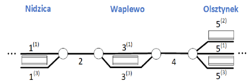
(a) Nidzica-Olsztynek section of railway line No. 216.

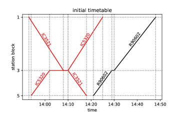
(b) Train diagram for the timetable of the line in Fig. 2(a).

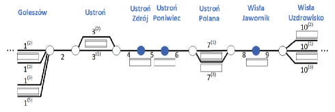
(c) Goleszów - Wisła Uzdrowisko section of railway line No. 191.

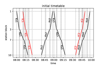
(d) Train diagram for the timetable of the line in Fig. 2(c).

Figure 2: The studied railway line segments and their initial (undisturbed) timetables.

Let us now turn our attention to the other example. The line segment (a part of railway line No. 191) is presented in Fig. 2(c), while the considered train paths of the real timetable are shown in Fig. 2(d). There are four stations and another three stops for the passengers modeled. Block $1$ represents Goleszów station, which has four platform edges. Block $2$ represents a line block between Goleszów station and Ustroń station (which has two platform edges and is represented by block $3$). Subsequently, we have three line blocks numbered $4$, $5$, and $6$, with two stops for passengers: Ustroń Zdrój and Ustroń Poniwiec (with one platform edge each). Next, we have station block $7$ – Ustroń Polana, which has two platform edges. Between this station and Wisła Uzdrowisko station (numbered $10$ with three platform edges), there are two more line blocks ($8$ and $9$) with one stop for passengers (Wisła Jawornik). We assume that it takes exactly the same time to get through a block regardless of the track used.

There are six trains, two Inter-City trains in red and four regional (KS) trains in black, presented in Fig. 2(d). The regional trains serve all the stops and stations, while the Inter-City service stops only at stations. We consider Wisła Uzdrowisko (station block $10$) to be a terminus for the Inter-City trains (however, it does not apply to the regional trains, which go farther). In this situation, there are no meet-and-pass situations at intermediate stations (Ustroń and Ustroń Polana) in the original timetable. Both Inter-City trains are served by the same train set, and the minimum service time is $R(j,j^{\prime})=20$ minutes at the terminus for ICs (block $10$); see Condition 3.4.

We analyze the following dispatching cases, selected to demonstrate the algorithm behavior in various situations:

1. A moderate delay of the Inter-City train setting off from station block $1$; see Fig. 12(a).

2. A moderate delay of all trains setting off from station block $1$; see Fig. 12(b).

3. A significant delay of some trains setting off from station block $1$; see Fig. 12(c).

4. A large delay of the Inter-City train setting off from station block $1$; see Fig. 12(d).

The conflicted timetables of cases $1-4$ are presented in Fig. 12.

5.2 Simple heuristics

In addition to using the linear job-shop model described in Section 3.4 for a comparison with a standard approach, we also present the solutions obtained with three simple heuristics, all prevalent in practice and resulting in feasible solutions: the FCFS, the FLFS, and the AMCC (avoid maximum current $C_{\text{max}}$) [19]. All of these heuristics are used to determine the order of trains when passing the blocks (for implementation reasons, the trains are analyzed in pairs). The FCFS and FLFS are rather simple, and they are common in real-life train dispatching around the world. In these heuristics, way is given to the train that first arrives – or first leaves – the analyzed block section. In practice, the decisions based on both these heuristics are taken starting from the most urgent conflict. Next, since passing and overtaking is possible only at stations, so-called implied selections [20] are determined. The procedure is repeated as long as all the conflicts are solved.

The AMCC is a more complex approach, whose objective is to minimize the maximum secondary delay of the trains; this objective will be referred to as the “AMCC objective” in what follows. This is quite an intuitive procedure, yet more sophisticated than FCFS and FLFS. To facilitate the comparison, stations are assigned an infinite capacity. Of course, solutions requiring a capacity higher than that of the given station must be rejected.

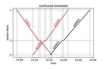
(a) The conflicted diagram.

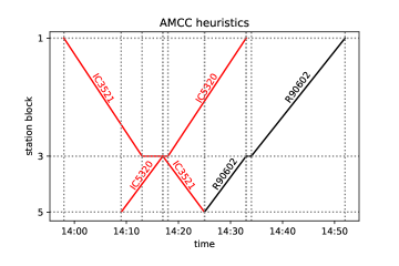
(b) The solution; FCFS, FLFS, and AMCC give the same outcome with a maximum seconday delay of $4$ minutes.

Figure 3: A possible solution of the conflict on line No. 216.

In the example presented in Fig. 2(a), for the conflicted timetable in Fig. 3(a), each of the heuristics returns the same solution; this is presented in Fig. 3(b). When comparing the FCFS with the FLFS, observe that in the conflicted timetable, three trains (IC$5320$, IC$5321$, R$90602$) are scheduled to occupy block $4$ simultaneously, which is forbidden.

To avoid the conflict, IC$5321$ is allowed to enter this block with a $3$-minute delay at 14:17 (as soon as IC$5320$ leaves the block), thus leaving the block at 14:25 instead of 14:22, which results in $3$ minutes of secondary delay. Consequently, R$9062$ is allowed to enter the block not earlier than 14:25, an additional $4$-minute delay as compared with the conflicted timetable. Thus the maximum secondary delay is $4$ minutes, and the sum of the delays on entering the last block is $7$ minutes. The maximum secondary delay is $4$ minutes; it is the lowest possible one, so the solution is optimal with respect to the AMCC objective.

The other example – presented in Fig. 2(c) – is more complex, yet it is still solvable by a state-of-the-art quantum annealer. We do not discuss this example in detail; we describe only the maximum secondary delays as the objective function. This is presented in Table 2 for the discussed heuristics. The upper limit used in the quantum computing is set to $d_{max}=10$ on this basis. (Observe that most of the secondary delay values are within this limit.) The respective train diagrams are presented in Appendix A, Figs. 13, 14, 15. The values of the AMCC objective function are presented in Table 2; AMCC appears to find the optimum in these cases, thus providing a good enough reference for comparisons, albeit with an objective function different from that of ours. Our choice of the objective will be more flexible, thus leaving room for further non-trivial optimization.

Heuristics	case $1$	case $2$	case $3$	case $4$
FLFS	6	13	4	2
FCFS	5	5	5	2
AMCC	5	5	4	2

Table 2: The maximum secondary delays, in minutes, resulting from simple heuristics. Observe that for each case, there are solutions far below $d_{\text{max}}=10$.

5.3 Quantum and calculated QUBO solutions

Our approach based on QUBO concerns the objective function set out in (56). This contains the feasibility conditions (hard constraints) and the objective function $f(\mathbf{x})$ of (64). For the feasibility part, we need to determine $\tau_{(1)}\left(j,s\right)$, the minimum time for train $j$ to give way to another train going in the same direction, and $\tau_{(2)}\left(j,s\right)$ - the minimum time for train $j$ to give way for the another train going in the opposite direction (see Condition 3.2 and Condition 3.3).

As noted before, the QUBO objective function introduces flexibility in choosing the dispatching policy by setting the values of the penalty weights for the delays of the trains. In this way, almost any train prioritization is possible. To demonstrate this flexibility, we make the penalty values proportional to the secondary delays of the trains that enter the last station block. This is equivalent to the secondary delay on leaving the penultimate station block. Each train is assigned a weight $w_{j}$, yielding the form of  (49):

$$f(\mathbf{x})=\sum_{j\in J}\left(\sum_{d\in A_{j,s^{*}}}w_{j}\cdot\frac{d(j,s^{*})-d_{U}(j,s^{*})}{d_{\text{max}}(j)}\cdot x_{j,s^{*},d}\right),$$ (64)

where $s^{*}=s_{(j,\text{end}-1)}$. Note that this objective coincides with that of the linear integer programming approach (39), which will be used for comparisons.

The following train prioritization is adopted. In the case of railway line No. 216, the Inter-City trains are assumed to have a higher value of the delay penalty weight $w=1.5$, while the regional train is weighted $w=1.0$. We give the higher priority to the Inter-City train, which is a reasonable approach resulting from the train prioritization in Poland (and in many other countries). In the other case (line No. $191$), the priorities of trains heading towards block $10$ (Wisła Uzdrowisko) are lower, weighted $0.9$ for all the other trains in this direction. However, train priorities for the trains heading in the opposite direction (toward block $1$ – Goleszów – and beyond the analyzed section) have higher values: $1.0$ for the regional trains and $1.5$ for the Inter-Cities. Such a policy is motivated by the reluctance of letting the delays propagate across the Polish railway network – that regional trains proceed toward the main railway junction in the region’s major city (Katowice) and that the Inter-City train service is scheduled toward the state’s capital city (Warsaw). Observe that $w_{j}$ is the highest possible penalty for the delay of train $j$; see (64). In both these cases, the maximum of $w_{j}$ is $1.5$. Hence, the penalties for a non-feasible solution should be higher; for a more detailed discussion, see Section 4.2. We set $p_{\text{pair}}=p_{\text{sum}}=1.75>1.5$.

Referring to (16), we have the maximum secondary delay $d_{\text{max}}$ parameter (for simplicity, we assume that $d_{\text{max}}$ is the same for all trains and all analyzed station blocks). It cannot be smaller than the delay value returned by the AMCC heuristics. However, since the AMCC may not be optimal in terms of our objective function, we need to leave a margin for some larger values of the maximum secondary delay. On the other hand, since the system size grows with $d_{max}$, it must be limited enough to make the problem applicable to state-of-the-art quantum devices and classical algorithms motivated by them. Specifically, since we do not analyze the delays at the last station of the analyzed segment of the line, we require as many as $(\text{number of station blocks}-1)\cdot(\text{number of trains})\cdot(d_{\text{max}}+1)$ qubits.

In the case of railway line No. $216$, we set $d_{\text{max}}=7$, which is considerably larger than the AMCC solution. There are $48$ logical quantum bits needed to handle this problem instance, making it suitable for both quantum annealing at the current state of the art, and the GPU-based implementation of the brute-force search for the low-energy spectrum (ground state and subsequent excited state) [3], which is possible with up to $50$ quantum bits. The benefit of this possibility is that it provides an exact picture of the spectrum, which can be used as a reference when evaluating the heuristic results of approximate methods (tensor networks) or quantum annealing. This may guide for the understanding of the results of the bigger instances, in which the brute-force exact search is not available.

There are many possible distinct solutions in the case of line No. $191$, making the analysis more interesting from the dispatching point of view. We set $d_{\text{max}}=10$: for a justification see Table 2, and observe that $d_{\text{max}}$ is considerably larger than the AMCC output. The $d_{\text{max}}=10$ yields $198$ logical quantum bits, which we were able to embed into a present-day quantum annealer, the D-Wave device DW-$2000\text{Q}_{5}$, in most cases.

Recall that current quantum annealing devices are imperfect and often output excited states. The clue of our approach is that the excited states (e.g., returned by the quantum annealer) still represent the optimal dispatching solutions, provided that their corresponding energies are relatively small. The reason for this is that what really needs to be determined is the order of trains leaving from each station block (i.e., this is the decision to be made). What is crucial here is to determine all the meet-and-pass and the meet-and-overtake situations (in analogy with the determination of all the precedence variables in the linear integer programming approach). The exact time of leaving block sections is of a secondary importance. Therefore, we consider those excited states that describe the same order of trains as the ground state, to be equivalent to the actual ground state encoding the global optimum. As discussed in Section 4.2, our QUBO formulation problem ensures that those equivalent solutions are part of the low-energy spectrum.

5.3.1 Exact calculation of the low-energy spectrum

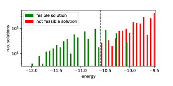
(a) $p_{\text{pair}}=2.7,p_{\text{sum}}=2.2$

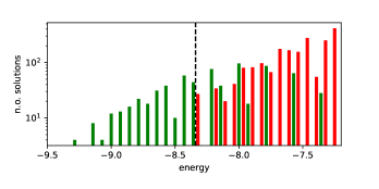
(b) $p_{\text{pair}}=p_{\text{sum}}=1.75$

Figure 4: Spectra of the low-energy solutions for two penalty strategies of the brute-force (exact) solution. The black line separates the phase in which only feasible solutions appear. Observe the mixing phase, in which both feasible and unfeasible solutions occur.

To demonstrate the aforementioned idea, we first present the results of the brute-force numerical calculations performed on a GPU architecture [3]. With this approach, the low-energy spectra of the smallest instances have been calculated exactly, providing some guidance for the understanding of the model behavior and parameter dependence. The method is suitable for small (i.e., up to $N\leq 50$ quantum bits) but otherwise arbitrary systems. To study (hard) penalties resulting from non-feasible solutions, apart from $p_{\text{pair}}=p_{\text{sum}}=1.75$ in  (56), we use other, higher penalties that are not equal to each other, $p_{\text{pair}}=2.7$ and $p_{\text{sum}}=2.2$.

Let us assume that the solution in Fig. 3(b) is the optimal one. Here the train IC$3521$ ($w=1.5$) waits $3$ minutes at block $3$, while regional train R$90602$ ($w=1.0$) waits $4$ minutes at block $5$, causing $4$ minutes of secondary delay upon leaving block $3$. This gives a penalty of $1.214$. Referring to the feasibility terms in (56), for a feasible solution $\mathcal{P}^{\prime}_{\text{sum}}=0$, while the linear constraint gives the negative offset to the energy. Referring to (55), as we have three trains for which we analyze two stations, this negative offset is $\mathcal{P}_{\text{sum}}=-3\cdot 2\cdot p_{\text{pair}}$. Based on the feasibility terms set out (56), this yields $-10.5$ for $p_{\text{sum}}=1.75$, and $-13.2$ for $p_{\text{sum}}=2.2$. This results in a ground state energy of $f^{\prime}(\mathbf{x})=-9.286$ and $f^{\prime}(\mathbf{x})=-11.986$, respectively. Finally, in the ground state solution shown in Fig. 3(b), the IC$3521$ train can leave the station block $1$ with a secondary delay of $0$, $1$, $2$, or $3$, not affecting any delays of the trains leaving block $3$. All these situations correspond to the ground state energy. Hence, our approach produces a $4$-fold degeneracy of the ground state.

Low-energy spectra of the solutions and their degeneracy are presented in Fig. 4(b) and Fig. 4(a). All the solutions that are equivalent to the ground state from the dispatching point of view are marked in green. Non-feasible excited state solutions [in which some of the feasibility conditions set out in (56) are violated] are marked in red. In this example, we do not have feasible solutions that are not optimal, i.e., in which the order of trains at a station is different from the one in the ground state solution.

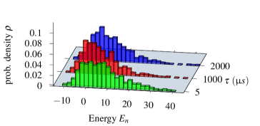
(a) QUBO parametrization: $p_{\text{pair}}=2.7,p_{\text{sum}}=2.2$.

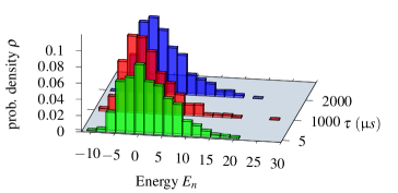
(b) $p_{\text{pair}}=p_{\text{sum}}=1.75$.

Figure 6: Distribution of the energies corresponding to the states (solutions), that are sampled by the D-Wave $2000$Q quantum annealer. In particular, $1000$ samples were taken for each annealing time, and the strength of embedding was set to $css=2.0$. This device is still very noisy and prone to errors, so the sample contains excited states.

In the case of line No. $191$, a more detailed analysis of the low-energy spectra of the solutions was possible due to the generality of the brute-force simulation. The results are presented in Fig. 4. We shall find later on that the D-Wave solutions managed to get into the “green” tail of feasible solutions, but high degeneracy of higher-energy states may impose some risk of the quantum annealing ending up in more frequently appearing excited states (see Fig. 6).

5.3.2 Classical algorithms for the linear (integer programming) IP model and QUBO

We expect classical algorithms for QUBOs to achieve the ground state of (56) or at least low excited states equivalent to the ground state with respect to the dispatching problem. It is important to mention that hereafter we transform the original QUBO coding into the Chimera graph coding (see Section 2.2.1). This makes the algorithm ready for processing on a real quantum annealer.

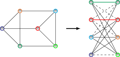
Figure 5: Embedding of a simple, six-qubit problem. Left: graph of the original problem. Right: problem embedded into a unit cell of Chimera. Here, different colors correspond to different logical variables. Apparently, the original problem does not map directly onto Chimera as it contains cycles of length 3. Therefore, two chains have to be introduced. Couplings corresponding to inner-chain penalties are marked with the same color as the variable they correspond to.

As to a simple example of the embedding, we refer to the problem with $4$ quantum bits that has been discussed in Section 4.3. In that case, the mapping was trivial. In a case of $6$ quantum bits, for instance (by setting $d_{\text{max}}=2$), we will have additional terms in (59), (60), and (61). Hence, the larger problems cannot be directly mapped onto the Chimera graph, so the embedding procedure is required, as illustrated in Fig. 5. This illustrates the basic idea of how the embedding is performed in even larger models.

As to the model parameters, recall that for the particular QUBO, we have opted for $p_{\text{pair}}=p_{\text{sum}}=1.75$ or $p_{\text{pair}}=2.2\ p_{\text{sum}}=2.7$ for line No. $216$ and $p_{\text{pair}}=p_{\text{sum}}=1.75$ for line No. $191$. Let us present the solutions of the two state-of-the-art numerical methods, which we shall later compare with the experimental results obtained by running the D-Wave $2000$Q quantum annealers. The first solver is developed ‘in-house’ and is based on tensor network techniques [53]. The idea behind this solver is to represent the probability of finding a given configuration by a quantum annealing processor as a PEPS tensor network [53]. This allows an efficient bound-and-branch strategy to be applied in order to find $M\ll 2^{N}$ candidates for the low-energy states, where $N$ is the number of physical quantum bits on the Chimera graph. In principle, such a heuristic method should work well for rather simple QUBO problems, i.e., those in which the $Q$ matrix in (6) has some identical or zero terms; this corresponds to the so-called weak entanglement regime. It can be shown that this is the case in our problem [see also the simple example of the $Q$ matrix in (62)]. Furthermore, heuristic parameters such as the Boltzmann temperature $(\beta)$ can be provided, allowing one to zoom in on the low-energy spectrum depending on the problem in question. We set $\beta=4$, which is quite a typical setting, as discussed in [53]. Although even better solutions may potentially be achieved by further tuning this parameter, we demonstrated that this default setting is satisfactory from the dispatching point of view. The second classical solver is CPLEX [62] (version 12.9.0.0). In our work, we have used the DOcplex Mathematical Programming package (DOcplex.MP) for Python. The results were compared with the linear integer programming approach, in which the model parameters were the same as for the QUBO formation.

We have also solved all our instances with the linear approach described in Section 3.4, to provide a fair comparison with a more traditional model. We have implemented this model with the PuLP package [63] and solved with its default solver (CBC MILP Solver Version: 2.9.0). All instances were solved to the optimal solution in 0.03 seconds on an average computer. This was in line with our expectations as our problems are small. Our goal is, however, not to outperform either CPLEX or the standard linear solver but to demonstrate the applicability of quantum hardware; at the present state of the art, we need the well-established solvers to produce results for comparisons and reference.

Concerning the results of another railway line (No. $191$), the values of the objective function  (64) are given Table 3. We also include the values of our objective function for the FLFS, FCFS, and AMCC optimal solutions. The slight advantage of AMCC and FCFS over the other methods in case $2$ is caused by the fact that (30) used in the QUBO (or linear integer programming approach) construction is an approximation and that in the block-to-block analysis the regional train Ks$4$ might have run a bit earlier, following the IC$2$ train. This, however, does not affect the optimality of the solution from the dispatching point of view.

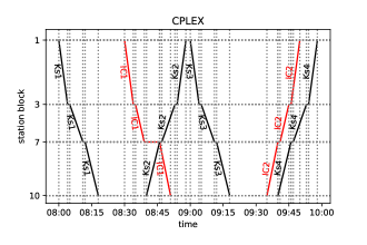
(a) Case $1$ – no “cascade effect” (Ks$2$ does not delay Ks$3$): a consequence of the pioritization of Ks$2$.

(b) Case $2$ – no uncacceptable stopovers.

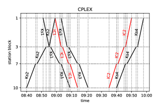
(c) Case $3$ – no unacceptable stopovers.

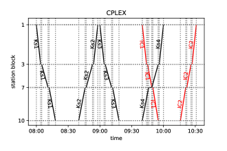
(d) Case $4$ – optimal solution according to all methods.

Figure 16: The CPLEX solutions: exact ground states of the QUBOs. There are no unacceptably long stopovers. Further, the trains’ prioritization and the delay propagation to subsequent trains are taken into account. The solutions are the same as these of the linear solver.

The agreement with the linear integer programming approach provides the argument that the CPLEX results refer to the ground state of the QUBO. We are interested in the results being equivalent to those of CPLEX and the linear solver from the dispatching point of view. These results are marked in blue in Table 3. The tensor network approach yields equivalent solutions to those of CPLEX. However, the tensor network sometimes returns the excited states of the QUBO, as can be observed in case $3$. This is caused by the fact that the tensor network method is based on approximations. This demonstrates that even some low-energy excited states encode a satisfactory solution. Interestingly, the results of the AMCC are also equivalent to those CPLEX in cases $2$,$3$, and $4$ but different in case $1$. This is due to the fact that the AMCC needs to have a specific objective function, whereas in our approach we can choose this function more flexibly. Specifically, in case $1$, the meet-and-pass situation of trains IC$1$ and Ks$2$ at station $10$ yields the lowest maximum secondary delay, so it is optimal from the AMCC point of view. (Note that two trains have secondary delays: Ks$2$ and Ks$3$ in this case). As discussed earlier, in this approach Ks$2$ is prioritized, as it is the train leaving the modeled network segment and one of the goals is to limit delays propagating further from this segment. The train diagrams based on the CPLEX solutions are depicted in Fig. 16.

In case $3$, observe that the objective function in Table 3 from the tensor network solution differs from the minimum (yet the solution is still equivalent to the optimal one). To explain this, observe that there are numerous possibilities of additional train delays that do not affect the dispatching situation. An example of such a situation is a train having its stopover extended at the station with no meet and pass or meet and overtake. Such a situation increases the value of the objective but does not affect the optimal dispatching solution. The number of combinations here is relatively high, and this is why such extended stopovers may be returned by the approximate algorithm. This is in contrast to the exact FCFS, FLFS, and AMCC heuristics, which do not allow for such unnecessary delays; the exact heuristics always return the $f(\mathbf{x})$ that is the minimum for the particular dispatching solution. In case $3$, the FCFS with $f(\mathbf{x})=0.95$ does not give the optimal solution from the dispatching point of view, as opposed to the tensor network with $f(\mathbf{x})=1.65$.

Method		case $1$	case $2$	case $3$	case $4$
QUBO approach	CPLEX	$\color[rgb]{0,0,1}0.54$	$\color[rgb]{0,0,1}1.40$	$\color[rgb]{0,0,1}0.73$	$\color[rgb]{0,0,1}0.20$
	tensor network	$\color[rgb]{0,0,1}0.54$	$\color[rgb]{0,0,1}1.40$	$\color[rgb]{0,0,1}1.65$	$\color[rgb]{0,0,1}0.29$
linear integer programming		$\color[rgb]{0,0,1}0.54$	$\color[rgb]{0,0,1}1.40$	$\color[rgb]{0,0,1}0.73$	$\color[rgb]{0,0,1}0.20$
Simple heuristics	AMCC	$0.77$	$\color[rgb]{0,0,1}1.30$	$\color[rgb]{0,0,1}0.73$	$\color[rgb]{0,0,1}0.20$
	FLFS	$\color[rgb]{0,0,1}0.54$	$1.71$	$\color[rgb]{0,0,1}0.73$	$\color[rgb]{0,0,1}0.20$
	FCFS	$0.77$	$\color[rgb]{0,0,1}1.30$	$0.95$	$\color[rgb]{0,0,1}0.20$

Table 3: The values of the objective function $f(\mathbf{x})$ for the solutions obtained by the classical calculation of the QUBO, linear integer programming approach, and all the heuristics. The blue color denotes equivalence from the dispatching point of view with the the ground state of the QUBO or the output of the linear integer programming. The equivalence concerns the same order of trains at each station.

5.3.3 Quantum annealing on the D-Wave machine

As described in Section 2.2.2, the solver we discuss (i.e., D-Wave $2000$Q quantum annealer) is probabilistic. In particular, as the required time to drive the system into its ground state is unknown, the output is a sample of the low-energy spectrum from repeated annealing processes, hence it can be regarded as a heuristic. The solution is thus assumed to be the element of this sample with the lowest energy (in practice, these elements are not from the ground states but from low excited states). The likelihood of obtaining solutions with a lower energy (or the actual ground state) increases with the number of repetitions.

As already mentioned, qubits on the D-Wave’s chip are arranged into a Chimera graph topology. Furthermore, some nodes and edges may be missing on the physical device, making the topology different even from an ideal Chimera graph. This requires minor embeddeding of the problem, mapping logical qubits onto physical ones. To this end, multiple physical qubits are chained together to represent a single logical variable, which increases their connectivity at the cost of the number of available qubits. Such embedding is performed by introducing an additional penalty term that favors states in which the quantum bits in each chain are aligned in the same direction. (Note that we encounter yet another penalty at this point.) The multiplicative factor governing this process is called the chain strength, and it should dominate all the coefficients present in the original problem. In this work, we set this factor to the maximum absolute value of the coefficients of the original problem multipled by a parameter that we call the chain strength scale (css). In our experiment, css ranged from $2.0$ to $9.0$. Another parameter is the annealing time (ranging from $5\upmu$s to $2000\upmu$s). This is the actual duration of the physical annealing process.

In Figs. 7(c) and 7(d), we present the energies of the best outcomes of the D-Wave machine for line No. $216$ and various annealing times. The green dots denote the feasible solutions (and equivalent to the optimal solution), while the red dots denote solutions that are not feasible. In general, the quality of a solution slightly rises with the annealing time; however, in large examples the best results are for a time somewhere between $1000\upmu$s and $2000\upmu$s. This coincides with the observation in [64], in which quantum annealing on the D-Wave machine was performed on various problems too, and it was demonstrated that for moderate problem size the performance (in terms of the probability of success) improves with an annealing time of up to $1000\upmu$s. Hence, we have limited ourselves to the annealing times of the order of magnitude of $1000\upmu$s in analyzing larger examples.

Rather counterintuitively, setting lower penalty coefficients of $p_{\text{sum}}=p_{\text{pair}}=1.75$ for the hard constraints, resulted in samples containing more feasible solutions. For this reason, we had kept this penalty setting for the analysis of the larger case. The embedding strength was set to $css=2$ in this case, i.e., the lowest possible value. This has proven to be a good choice, as demonstrated in Fig. 8. The best D-Wave solutions are presented in the form of train diagrams in Figs. 7(a) and 7(b).

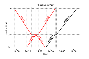
(a) The optimal solution from Fig. 7(c).

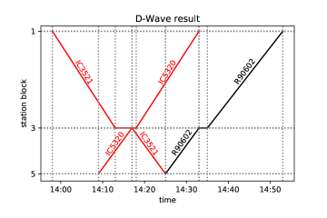
(b) The optimal solution from Fig. 7(d).

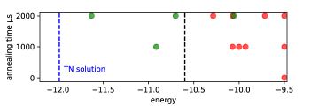
(c) $p_{\text{pair}}=2.7,p_{\text{sum}}=2.2$.

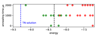
(d) $p_{\text{pair}}=p_{\text{sum}}=1.75$.

Figure 7: Train diagrams of the best D-Wave solutions, the lowest energies of the quantum annealing on the D-Wave machine (green: feasible, red: not feasible), and the optimal tensor network solution.

The quality of the solutions in relation to the css strength in the various parameter settings is presented in Fig. 8. We observed that in our cases, the quality of the solution degraded with an increase in css. This is unusual, as increasing the css strength typically yields more solutions without broken chains that do not need to be post-processed to obtain a feasible solution of the original problem. This may be caused by the fact that the large coupling of the embedding may cause the constraints to appear as a small perturbation in the physical QUBO. These perturbations, as discussed earlier, may be hidden in the noise of the D-Wave $2000$Q annealer.

Hence, we set $css=2.0$ (the lowest possible value) for the further investigations. Some examples of the penalty and objective function values are presented in Table 4. Again, it appears that the higher the values of $p_{\text{sum}}$ and $p_{\text{pair}}$, the higher the values of $f(\mathbf{x})$. This may be caused by the objective function being lost in the noise of the D-Wave $2000$Q annealer.

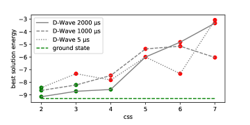
(a) The minimal energies vs. css for $p_{\text{pair}}=1.75,p_{\text{sum}}=1.75$.

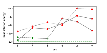
(b) The minimal energies vs. css for $p_{\text{pair}}=2.2,p_{\text{sum}}=2.7$.

Figure 8: Line No. 216, with the minimal energy from the D-Wave quantum annealer, using $1000$ runs. Green dots indicates the feasible solutions, while the red dots denote the unfeasible ones. In general, the energy rises as the css strength rises. We do not observe that the different settings of $p_{\text{pair}}$ and $p_{\text{sum}}$ improve the feasibility; see Fig. 8(b).

For railway line No. 191, finding the feasible solution is more difficult. Hence, we took advantage of the maximal number of runs on the D-Wave machine, which equals $250\ 000$ runs. The results of the lowest energies and penalties are presented in Fig. 9. We had to skip case $3$ because the higher number of feasibility constraints prevented finding any embedding on a real Chimera. Interestingly, recall that we found the embedding for the ideal Chimera while simulating the solution (see Section 5.3.2). Hence, the failure in the case of the real graph is possibly caused by the fact that some of the required connections or nodes are missing from the real Chimera. Finding the feasible solution in such a case (while having non-zero hard constraints penalties) is a problem for further research. One would expect that increasing the $p_{\text{pair}}$ and $p_{\text{sum}}$ parameters could be helpful. However, it may aggravate the objective function to an ever greater extend. In Fig. 9(b), the values of the objective function $f(\mathbf{x})$ are much higher than the optimal ones presented in Table 3.

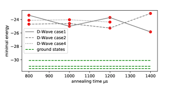
(a) Best D-Wave solutions (these are the lowest excited states we have recorded). Red dots indicate that the solutions are not feasible.

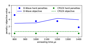
(b) Comparison of the objective and hard penalty between the D-Wave outcome and the expected bahaviour (supplied by the CPLEX).

Figure 9: Line No. 191, with the minimal energy from the D-Wave annealer at $250$k runs, css = $2.0$, and $p_{\text{pair}}=1.75,p_{\text{sum}}=1.75$. The output does not dependent on the annealing time (in the investigated range) and is still far from the ground state.

css	$p_{\text{sum}},p_{\text{pair}}$	hard constraints’ penalty $f^{\prime}(\mathbf{x})$	$f(\mathbf{x})$
$2$	$1.75,1.75$	$0.0$	$1.36$
$2$	$2.2,2.7$	$0.0$	$1.57$
$4$	$1.75,1.75$	$0.0$	$1.93$
$4$	$2.2,2.7$	$2.2$	$2.07$
$6$	$1.75,1.75$	$5.25$	$0.43$
$6$	$2.2,2.7$	$6.6$	$0.86$

Table 4: Line No. 216, with the objective functions and penalties for violating the hard constraints: see (57). Output from the D-Wave quantum annealer, for the annealing time of $2000\upmu$s. If $f^{\prime}(\mathbf{x})>0$, the solution is not feasible. The $p_{\text{sum}}=p_{\text{pair}}=1.75$ policy gives lower objectives.

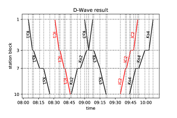
(a) Case $1$.

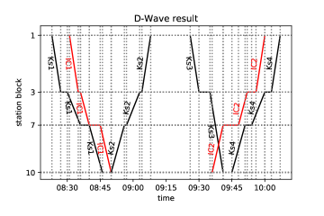
(b) Case $2$.

Figure 10: The best solutions obtained from the D-Wave quantum annealer for line No. 191. For case 1 (Fig. 10(a)), the annealing time is $t=1400$. The solution is unfeasible since the stay of Ks$3$ at station $7$ is below $1$ minute. If the solution is corrected (i.e., the stay is introduced), it looses its optimailty and reflects a dispatching situation different from those obtained from FCFS, FLFS, AMCC, CPLEX, or the tensor network. For case $2$ (Fig. 10(b)), $t=1200$ is used. The solution is unfeasible as Ks$3$ does not stop at station $7$; hence, Ks$3$ and IC$2$ are supposed to meet and pass between stations $7$ and $10$. It can, however, be amended to an optimal solution: shortening the stay of Ks$3$ at station $3$ and shortening the stay of IC$2$ at station $7$ (and $3$ if necessary) result in a meet-and-pass situation at station $10$, and this is optimal.

Although the solutions are not feasible, we select the two in which only one hard constrain is violated ($f^{\prime}(\mathbf{x})=1.75$); these are case $1$ with an annealing time of $1400\upmu$s, and case $2$ with an annealing time of $1200\upmu$s. The train diagrams of these solutions are presented in Fig. 10. Note that both these diagrams can easily be modified by the dispatcher to obtain a feasible solution. The case in Fig. 10(a) can be amended by adding the lacking $1$-minute stay of Ks$3$ in station $7$. Here the solution would not be optimal, and it would be different from the optimal one from CPLEX, the tensor network, and FLFS, as well as from the non-optimal yet feasible ones returned by FCFS and AMCC. The case in Fig. 10(b) can be upgraded by shortening the stays of Ks$3$ and IC$2$ and letting them meet and pass at station $10$. Here the solution would be optimal and equivalent to those achieved with the tensor networks and CPLEX.

The real D-Wave quantum annealing is tied to some parameters of both the particular QUBO and the machine itself. We achieved the best results for a coupling constant css = $2.0$ for the small example in Fig. 8(a); the same observation was made for the large example. This was not expected as the coupling between quantum bits representing a single classical bit was rather weak. Here we probably took advantage of the possible variations within the realization of a logical bit. This observation demonstrates that the embedding selection may be meaningful in searching for the convergence toward proper solutions lying in the low-energy part of the spectrum. For the small cases, we observed a feasible solution for a relatively small number of samples (equal to $1$k). For the larger case, the number of samples had to be increased to the maximal possible (equal to $250$k) and still we did not reach any feasible solution. The conclusion is that the impact of the noise amplifies strongly with the size of the problem. The convergence of the best obtained solution toward the optimal one with the given sample size is complex, and an in-deep statistical analysis of sampling the annealer’s real distribution is required.

As demonstrated in Fig 9(b), for some cases only a single hard constraint was broken. This may suggest that we are near the region of feasible solutions. However, the objective function values are still far from the optimal ones achieved by means of simulations (see Table 3). To elucidate the interplay between penalties, we refer to Fig. 10, in which the solutions are not feasible but can be easily corrected by the dispatcher to obtain feasible ones. In Fig. 10(b), the corrected solution would be optimal, while in Fig. 10(a) it would not be different from all the other achieved solutions. Hence, the current quantum annealer would rather sample the excited part of the QUBO spectrum, which can lead to unusual solutions. Such solutions, however, can be still be used by the dispatcher for some particular reason not encoded directly in the model. Such reasons include unexpected dispatching problems, rolling stock emergency, and non-standard requirements.

Let us also mention the characteristics of our QUBO problems as they are important features from the point of view of quantum methods. Table 5 summarizes the problem sizes and the densities of edges in the case of each problem instance.

Features	line 216	line 191
		case $1$	case $2$	case $3$	case $4$	enlarged
problem size ($\#$ logical bits)	$48$	$198$	$198$	$198$	$198$	$594$
$\#$ edges	$395$	$1851$	$2038$	$2180$	$1831$	$5552$
density (vs. full graph)	$0.35$	$0.095$	$0.104$	$0.111$	$0.094$	$0.032$
3 embedding into	Chimera	Chimera	Chimera	Ideal Chimera	Chimera	Pegasus
approximate $\#$ physical bits	$373$	$<2048$	$<2048$	$\approx 2048$	$<2048$	$<5760$

Table 5: Graph densities for various problems. As case $3$ is supposed to be the most complicated one of cases $1-4$, it has the largest graph density.

5.4 Initial studies on the D-Wave Advantage machine

During the preparation of the present paper, a new quantum device, the D-Wave’s Advantage_system1.1 system (with an underlying topology code-named Pegasus [1]) became commercially available. Hence, we performed preliminary experiments with this new architecture to address a slightly larger example. To that end, we expanded our initial Goleszów – Wisła Uzdrowisko (line No. $191$) problem instance to be $3$ times bigger in size. Furthermore, we investigated nine trains in each direction.

The conflicts were introduced by assuming delays of $20$, $25$, or $30$ minutes of certain trains entering block section $1$. The control parameters’ values $p_{\text{sum}}=p_{\text{pair}}=1.75$ and $css=2$ were not changed. As a result, the problem was mapped onto a QUBO with $594$ variables and $5552$ connections. This new setup changed the underlying embedding only slightly, and we omit a discussion of the details here. Employing a strategy similar to the one used for our other calculations, we used the solution found by CPLEX as a reference for comparisons.

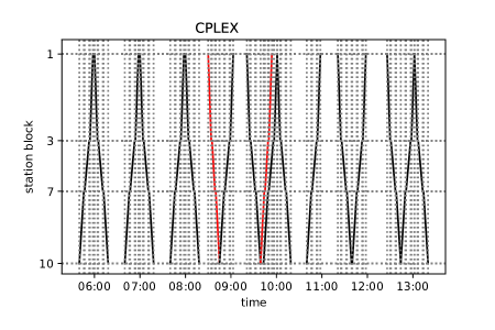
Figure 11: The CPLEX QUBO solution, coinciding with the linear solver’s solution of the $18$-train problem.

After performing $25$k runs, we reached a minimal energy of $+75.28$ with an annealing time of $1400\upmu$s. Unfortunately, this is not a feasible solution. The CPLEX calculations, on the other hand, resulted in an energy of $-92.43$ with an objective function value $f(\mathbf{x})=2.07$ (see Fig. 11). This is the same solution as the solution of the linear solver obtained using COIN-OR in 0.02 seconds. This solution is substantially better, and as it coincides with the linear solver’s output, it corresponds to the ground state. Our preliminary experiments indicate the need for a more detailed investigation of the new device’s behavior (and that of the current model) to determine whether obtaining solutions with the desired (better) quality is possible. A part of this problem will likely be eliminated simply by the technological development of the new annealer. For an intuitive justification, we refer to [65] and Fig. $1$ therein, in which an improvement in the performance between subsequent iterations within one generation of Chimera-based quantum annealers was observed.

6 Discussion and conclusions

We have introduced a new approach to the single-track line dispatching problem that can be implemented on a real quantum annealing device (D-Wave $2000$Q). We have addressed two particular real-life railway dispatching problems in Poland; many similar examples exist in other networks, too. We have introduced a QUBO model of the problem that can be solved with quantum annealing. We have solved our model with quantum annealers as well as with classical algorithms. We have compared the solutions with the results from simple heuristics and a linear integer programming formulation of our model, in line with standard dispatching models.

The first dispatching problem we considered (the Nidzica – Olsztynek section of line No. $216$) was particularly small, so it was defined using $48$ logical quantum bits (which we were able to embed into $373$ physical quantum bits of a real quantum processor). The final state reached by the quantum annealer for this problem was optimal for many parameter settings. This highlights that small-sized dispatching problems are already within reach of near-term quantum annealers. In addition, the limited size of the problem made it possible to analyze the QUBO with a greedy brute-force search algorithm, which revealed details of the behavior of the spectrum that cannot be exactly calculated for bigger instances.

Our second set of dispatching problems (the Goleszów – Wisła Uzdrowisko section of line No. $191$) was larger and needed $198$ logical quantum bits. Here, the number of physical quantum bits depends on the number of constraints in each of the analyzed cases. We were able to embed all four dispatching cases of the No. $191$ railway line into an ideal Chimera graph ($2048$ physical quantum bits) using a state-of-the-art embedding algorithm. We succeeded in solving these instances with classical solvers for QUBOs. Meanwhile, on the physical device (whose graph is not perfect and lacks several quantum bits and couplings), we were able to embed only three out of the four cases (case $3$, with the highest number od conflicts, could not be embedded). We expect that such obstacles will become less restrictive as new embedding algorithms are being developed for both the current Chimera topology and the newest D-Wave Pegasus; see [66, 67]. Therefore, it is not unreasonable to expect that the range of problems that can be embedded so that they can be solved on physical hardware will substantially increase in the near future. Unfortunately, the D-Wave $2000$Q solutions of our second problem appeared to be far from optimal. This is attributable to the noise that is still present in the current quantum machine.

We have successfully solved our model using certain algorithms for QUBOs running on classical computers, notably the novel tensor network method. This introduces additional possibilities, namely, that of QUBO modeling and the use of quantum-motivated classical algorithms. Although these possibilities obviously do not promise a breakthrough in scalability, they are essential for the validation and assessment of the results of real quantum annealing. In addition, they can yield practically useful results.

We are aware that the examples of the single-track railway dispatching problem discussed in the paper can be regarded as trivial from the point of view of professional dispatchers. This is also reflected by the efficiency of the conventional linear solver they may use. Our intention, however, was to provide a proof-of-concept demonstration of the applicability of quantum annealing in this field. This goal has been achieved: we have described a suitable model and succeeded in solving certain instances.

Due to the small size of the current quantum annealing processors, our implementation is limited: quantum annealing is an emerging technology. Owing to the significant efforts put into the development of quantum annealers, the addressable problem sizes are about to increase, and the quality of the samples will also improve. With the development of the technology, it cannot be excluded that at some point quantum annealers will be able to compete with or even outperform classical solvers. Another possible research direction is a combination of D-Wave with other classical techniques and to use D-Wave for solving certain subproblems instead of formulating a complete job-shop model such as a QUBO. Such a combination may possibly perform better, which is a subject of ongoing research.

7 Acknowledgments

This work was supported by the National Research, Development, and Innovation Office of Hungary under project numbers K133882, K124351, and 2017-1.2.1-NKP-2017-00001 HunQuTech; and the Foundation for Polish Science (FNP) under grant number TEAM NET POIR.04.04.00-00-17C1/18-00 (KD and BG); and the National Science Centre (NCN), Poland, under project number 2016/22/E/ST6/00062 (KJ). We gratefully acknowledge the support of NVIDIA Corporation which donated the Titan V GPU used for this research. We acknowledge the language corrections performed by ProofreadingServices.com

Appendix A Appendix

In the appendix, we present all the solutions of the dispatching problems on line No. $191$ obtained by our algorithms. Both the CPLEX and tensor network approaches (which are based on QUBO) allow for rather arbitrary decisions on train prioritization. These approaches focus on the train delay propagation on subsequent trains, as illustrated by the comparison of all the solutions of case $1$. Provided Ks$2$ is delayed, an additional delay of Ks$3$ would happen (which we call a “cascade effect”). Furthermore, the tensor network output in Fig. 17 demonstrates the degeneracy of the ground state and the solutions in the low excited state, which, however, do not have a relevant impact on the dispatching situation. (In our cases all CPLEX solutions ar the same as these of the linear solver.)

Note that the simple heuristics (FCFS, FLFS) sometimes return trouble-causing solutions. This situation suggests a solution in which one train needs to have a time-consuming stopover on a particular station; see Figs. 13(c),14(b). (Such problems sometimes appear in real-life train dispatching too.) Finally, if the problem is easily solvable, as in case $4$, all the methods analyzed in the paper give the same solution. This serves as a quality test of our method.

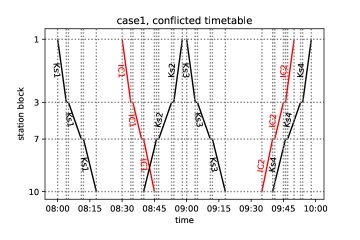
(a) Case $1$ – single conflict, observe that the additinal delay of Ks$2$ will propagate to the delay of Ks$3$.

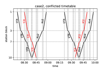
(b) Case $2$ – two conflicts, simillar to Fig. 12(a), but with no impact of Ks$2$ on Ks$3$.

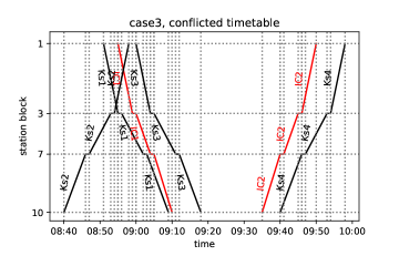
(c) Case $3$ – multiple conflicts.

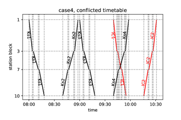
(d) Case $4$ – conflict that is straightforward to resolve.

Figure 12: The conflicted timetables, various types of conflicts.

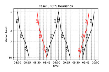
(a) Case $1$ – “cascade effect”; the delay of Ks$2$ causes a further delay of Ks$3$.

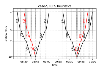
(b) Case $2$ – optimal solution reached rather “at random”: probably it is reached because the peoblem is relativelly simple.

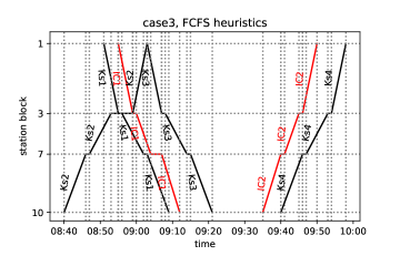
(c) Case $3$ – a problematic solution with undesirably long waiting times of certain trains; observe the stopover of Ks$2$.

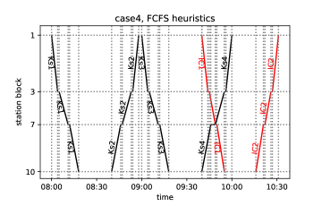
(d) Case $4$ – optimal solution according to all methods.

Figure 13: The FCFS solutions, some with a trouble-causing stopover of a particular train.

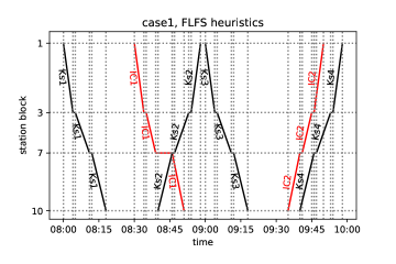
(a) Case $1$ – optimal solution is reached “at random,” as is its duplicate in Fig. 14(b), which is an undesired solution.

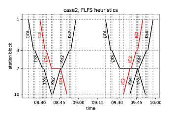
(b) Case $2$ – duplicate of the solution in Fig. 14(a) causing an stopover of Ks$3$.

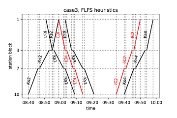
(c) Case $3$ – no unacceptable stopovers.

(d) case $4$ – optimal solution according to all methods.

Figure 14: The FLFS solutions, some with a trouble-causing stopover of a particular train.

(a) Case $1$ – “cascade effect,” the delay of Ks$2$ causes further a delay of Ks$3$.

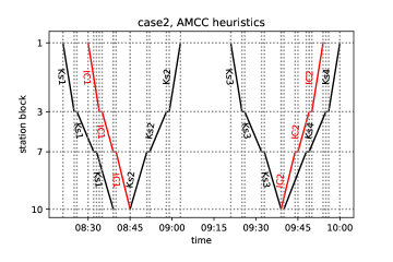
(b) Case $2$ – no unacceptable stopovers.

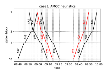
(c) Case $3$ – no unacceptable stopovers

(d) Case $4$ – optimal solution according to all methods.

Figure 15: The AMCC solutions. The minimization of the maximal secondary delays from AMCC excludes unacceptably long stopovers such as those in Figs. 13(c) and 14(b). However, these solutions do not exclude the propagation of smaller delays among several trains (“cascade effect”); see Fig. 15(a).

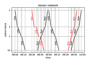
(a) Case $1$ – ground state of the QUBO; the degeneracy of the ground state is reflected by a stay of IC$1$ both at block $3$ and at block $7$.

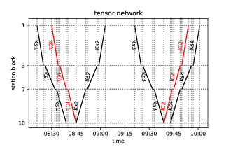
(b) Case $2$ – ground state of the QUBO.

(c) Case $3$ – excited state of the QUBO; notice the slightly longer stay of IC$1$ at block $7$.

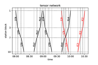
(d) Case $4$ – excited state of the QUBO; notice the slightly longer stay of Ks$3$.

Figure 17: The tensor network solutions; although the exact ground states were not always achieved, the solutions are equivalent from the dispatching point of view with to in Fig. 16.

References

- [1] N. Dattani, S. Szalay, and N. Chancellor, “Pegasus: The second connectivity graph for large-scale quantum annealing hardware.” e-print arXiv:1901.07636, 2019.
- [2] P. A. R. Ade et al., “Planck 2015 results - XIII. Cosmological parameters,” Astron. Astrophys., vol. 594, p. A13, 2016.
- [3] K. Jałowiecki, M. M. Rams, and B. Gardas, “Brute-forcing spin-glass problems with CUDA,” Comput. Phys. Commun, vol. 260, 11/2020 2021.
- [4] T. Lanting et al., “Entanglement in a quantum annealing processor,” Phys. Rev. X, vol. 4, p. 021041, 2014.
- [5] J. Törnquist and J. A. Persson, “N-tracked railway traffic re-scheduling during disturbances,” Transportation Research Part B: Methodological, vol. 41, no. 3, pp. 342 – 362, 2007.
- [6] L. Lamorgese, C. Mannino, D. Pacciarelli, and J. T. Krasemann, Train Dispatching, in Handbook of Optimization in the Railway Industry, pp. 265–283. Cham: Springer International Publishing, 2018.
- [7] J. Jensen, O. Nielsen, and C. Prato, “Passenger perspectives in railway timetabling: A literature review,” Transport Reviews, vol. 36, no. 4, pp. 500–526, 2016.
- [8] C. Wen, P. Huang, Z. Li, J. Lessan, L. Fu, C. Jiang, and X. Xu, “Train dispatching management with data- driven approaches: A comprehensive review and appraisal,” IEEE Access, vol. 7, pp. 114547–114571, 2019.
- [9] X. Cai and C. J. Goh, “A fast heuristic for the train scheduling problem,” Computers & Operations Research, vol. 21, no. 5, pp. 499 – 510, 1994.
- [10] B. Szpigel, “Optimal train scheduling on a single line railway,” Operational Research, vol. 72, pp. 343–352, 1973.
- [11] M. L. Pinedo, Scheduling: Theory, Algorithms, and Systems. Springer Publishing Company, Incorporated, 3rd ed., 2008.
- [12] J.-F. Cordeau, P. Toth, and D. Vigo, “A survey of optimization models for train routing and scheduling,” Transportation Science, vol. 32, p. 380–404, Apr. 1998.
- [13] J. Törnquist, “Computer-based decision support for railway traffic scheduling and dispatching: A review of models and algorithms,” in 5th Workshop on Algorithmic Methods and Models for Optimization of Railways (ATMOS’05), Schloss Dagstuhl-Leibniz-Zentrum für Informatik, 2006.
- [14] T. Dollevoet, D. Huisman, M. Schmidt, and A. Schöbel, Delay Propagation and Delay Management in Transportation Networks, pp. 285–317. Cham: Springer International Publishing, 2018.
- [15] F. Corman and L. Meng, “A review of online dynamic models and algorithms for railway traffic management,” IEEE Transactions on Intelligent Transportation Systems, vol. 16, no. 3, pp. 1274–1284, 2015.
- [16] V. Cacchiani and P. Toth, “Nominal and robust train timetabling problems,” European Journal of Operational Research, vol. 219, no. 3, pp. 727 – 737, 2012.
- [17] I. Hansen, State-of-the-art of railway operations research, pp. 35–47. United Kingdom: WIT Press, 2010.
- [18] J. Lange and F. Werner, “Approaches to modeling train scheduling problems as job-shop problems with blocking constraints,” J Sched, vol. 21, no. 2, pp. 191–207, 2018.
- [19] A. Mascis and D. Pacciarelli, “Job-shop scheduling with blocking and no-wait constraints,” European Journal of Operational Research, vol. 143, no. 3, pp. 498–517, 2002.
- [20] A. D’Ariano, D. Pacciarelli, and M. Pranzo, “A branch and bound algorithm for scheduling trains in a railway network,” European Journal of Operational Research, vol. 183, no. 2, pp. 643–657, 2007.
- [21] D. Venturelli, D. J. J. Marchand, and G. Rojo, “Quantum annealing implementation of job-shop scheduling,” 2015. e-print arXiv:1506.08479.
- [22] X. Zhou and M. Zhong, “Single-track train timetabling with guaranteed optimality: Branch-and-bound algorithms with enhanced lower bounds,” Transportation Research Part B: Methodological, vol. 41, no. 3, pp. 320–341, 2007.
- [23] S. Harrod, “Modeling Network Transition Constraints with Hypergraphs,” Transportation Science, vol. 45, no. 1, pp. 81–97, 2011.
- [24] L. Meng and X. Zhou, “Simultaneous train rerouting and rescheduling on an N-track network: A model reformulation with network-based cumulative flow variables,” Transportation Research Part B: Methodological, vol. 67, pp. 208–234, 2014.
- [25] T. Kadowaki and H. Nishimori, “Quantum annealing in the transverse Ising model,” Phys. Rev. E, vol. 58, pp. 5355–5363, 1998.
- [26] D. Aharonov, W. van Dam, J. Kempe, Z. Landau, S. Lloyd, and O. Regev, “Adiabatic quantum computation is equivalent to standard quantum computation,” in 45th Annual IEEE Symposium on Foundations of Computer Science, pp. 42–51, 2004.
- [27] M. A. Nielsen and I. L. Chuang, Quantum Computation and Quantum Information: 10th Anniversary Edition. Cambridge, UK: Cambridge University Press, 2010.
- [28] J. D. Biamonte and P. J. Love, “Realizable Hamiltonians for universal adiabatic quantum computers,” Phys. Rev. A, vol. 78, p. 012352, 2008.
- [29] A. Lucas, “Ising formulations of many NP problems,” Front. Phys., vol. 2, p. 5, 2014.
- [30] T. Albash and D. A. Lidar, “Adiabatic quantum computation,” Rev. Mod. Phys., vol. 90, p. 015002, 2018.
- [31] F. Glover, G. Kochenberger, and Y. Du, “Quantum Bridge Analytics I: A tutorial on formulating and using QUBO models,” 4OR-Q J Oper Res, vol. 17, no. 4, pp. 335–371, 2019.
- [32] M. Aramon, G. Rosenberg, E. Valiante, T. Miyazawa, H. Tamura, and H. G. Katzgraber, “Physics-inspired optimization for quadratic unconstrained problems using a digital annealer,” Front. Phys., vol. 7, p. 48, 2019.
- [33] D. Pierangeli, M. Rafayelyan, C. Conti, and S. Gigan, “Scalable spin-glass optical simulator.” e-print arXiv:2006.00828, 2020.
- [34] Y. Yamamoto, K. Aihara, T. Leleu, K. Kawarabayashi, S. Kako, M. Fejer, K. Inoue, and H. Takesue, “Coherent Ising machines—optical neural networks operating at the quantum limit,” Npj Quantum Inf., vol. 3, no. 1, p. 49, 2017.
- [35] B. H. Fukushima-Kimura, S. Handa, K. Kamakura, Y. Kamijima, and A. Sakai, “Mixing time and simulated annealing for the stochastic cellular automata.” eprint arXiv:2007.11287, 2020.
- [36] F. Cai et al., “Power-efficient combinatorial optimization using intrinsic noise in memristor Hopfield neural networks,” Nat. Electron., vol. 3, no. 7, pp. 409–418, 2020.
- [37] J. E. Avron and A. Elgart, “Adiabatic theorem without a gap condition,” Commun. Math. Phys., vol. 203, no. 2, pp. 445–463, 1999.
- [38] I. Ozfidan et al., “Demonstration of nonstoquastic Hamiltonian in coupled superconducting flux qubits.” e-print arXiv:1903.06139, 2019.
- [39] V. Choi, “Minor-embedding in adiabatic quantum computation: I. The parameter setting problem,” Quantum Inf. Process., vol. 7, no. 5, pp. 193–209, 2008.
- [40] R. Hamerly et al., “Experimental investigation of performance differences between coherent Ising machines and a quantum annealer,” Sci. Adv., vol. 5, no. 5, 2019.
- [41] A. D. King, W. Bernoudy, J. King, A. J. Berkley, and T. Lanting, “"Emulating the coherent Ising machine with a mean-field algorithm".” e-print arXiv:1806.08422v1, 2018.
- [42] T. Onodera, E. Ng, and P. L. McMahon, “A quantum annealer with fully programmable all-to-all coupling via Floquet engineering.” e-print arXiv:math-ph/0409035, 2019.
- [43] A. M. Childs, E. Farhi, and J. Preskill, “Robustness of adiabatic quantum computation,” Phys. Rev. A, vol. 65, p. 012322, 2001.
- [44] H. G. Katzgraber, F. Hamze, Z. Zhu, A. J. Ochoa, and H. Munoz-Bauza, “Seeking quantum speedup through spin glasses: The good, the bad, and the ugly,” Phys. Rev. X, vol. 5, p. 031026, 2015.
- [45] S. Sachdev, Quantum Phase Transitions. Cambridge University Press, 2011.
- [46] J. Dziarmaga, “Dynamics of a quantum phase transition: Exact solution of the quantum Ising model,” Phys. Rev. Lett., vol. 95, p. 245701, 2005.
- [47] J. Dziarmaga, “Dynamics of a quantum phase transition and relaxation to a steady state,” Adv. Phys., vol. 59, no. 6, pp. 1063–1189, 2010.
- [48] T. W. B. Kibble, “Topology of cosmic domains and strings,” J. Phys. A: Math. Gen., vol. 9, p. 1387, 1976.
- [49] T. W. B. Kibble, “Some implications of a cosmological phase transition,” Phys. Rep., vol. 67, no. 1, pp. 183 – 199, 1980.
- [50] W. H. Zurek, “Cosmological experiments in superfluid helium?,” Nature, vol. 317, p. 505, 1985.
- [51] U. Schollwöck, “The density-matrix renormalization group,” Rev. Mod. Phys., vol. 77, pp. 259–315, Apr 2005.
- [52] F. Verstraete and J. I. Cirac, “Matrix product states represent ground states faithfully,” Phys. Rev. B, vol. 73, p. 094423, Mar 2006.
- [53] M. M. Rams, M. Mohseni, and B. Gardas, “Heuristic optimization and sampling with tensor networks,” 2018. e-print arXiv:1811.06518.
- [54] J. Czartowski, K. Szymański, B. Gardas, Y. V. Fyodorov, and K. Życzkowski, “Separability gap and large-deviation entanglement criterion,” Phys. Rev. A, vol. 100, p. 042326, 2019.
- [55] I. Sax, S. Feld, S. Zielinski, T. Gabor, C. Linnhoff-Popien, and W. Mauerer, “Approximate approximation on a quantum annealer,” in Proceedings of the 17th ACM International Conference on Computing Frontiers, pp. 108–117, 2020.
- [56] T. Stollenwerk, B. O’Gorman, D. Venturelli, S. Mandrà, O. Rodionova, H. Ng, B. Sridhar, E. G. Rieffel, and R. Biswas, “Quantum annealing applied to de-conflicting optimal trajectories for air traffic management,” IEEE Transactions on Intelligent Transportation Systems, vol. 21, no. 1, pp. 285–297, 2020.
- [57] Y. Jing, Y. Liu, and M. Bi, “Quantum-inspired immune clonal algorithm for railway empty cars optimization based on revenue management and time efficiency,” Cluster Computing, vol. 22, pp. 545–554, 2019.
- [58] D. Luenberger and Y. Ye, Linear and Nonlinear Programming. International Series in Operations Research & Management Science, Springer International Publishing, 2015.
- [59] I. Hen and F. M. Spedalieri, “Quantum annealing for constrained optimization,” Phys. Rev. Applied, vol. 5, p. 034007, Mar 2016.
- [60] “DWave Ocean Software Documentation.” https://docs.ocean.dwavesys.com/en/stable. Accessed: 2020-06-29.
- [61] PKP Polskie Linie Kolejowe S.A., “Public procurement website.” https://zamowienia.plk-sa.pl/.
- [62] “CPLEX optimizer.” https://www.ibm.com/analytics/cplex-optimizer. Accessed: 2020-06-29.
- [63] “Optimization with PuLP.” https://coin-or.github.io/pulp. Accessed: 2021-02-15.
- [64] R. Hamerly, T. Inagaki, P. L. McMahon, D. Venturelli, A. Marandi, T. Onodera, E. Ng, C. Langrock, K. Inaba, T. Honjo, et al., “Experimental investigation of performance differences between coherent Ising machines and a quantum annealer,” Science Advances, vol. 5, no. 5, p. eaau0823, 2019.
- [65] K. Jałowiecki, A. Więckowski, P. Gawron, and B. Gardas, “Parallel in time dynamics with quantum annealers,” Scientific Reports, vol. 10, no. 1, pp. 1–7, 2020.
- [66] S. Zbinden, A. Bärtschi, H. Djidjev, and S. Eidenbenz, “Embedding algorithms for quantum annealers with chimera and pegasus connection topologies,” in International Conference on High Performance Computing, pp. 187–206, Springer, 2020.
- [67] E. Pelofske, G. Hahn, and H. Djidjev, “Decomposition algorithms for solving np-hard problems on a quantum annealer,” Journal of Signal Processing Systems, pp. 1–16, 2020.