Complexity of dipolar exciton Mott transition in GaN/(AlGa)N nanostructures

Abstract

The Mott transition from a dipolar excitonic liquid to an electron-hole plasma is demonstrated in a wide GaN/(Al,Ga)N quantum well at $T=7$ K by means of spatially-resolved magneto-photoluminescence spectroscopy. Increasing optical excitation density we drive the system from the excitonic state, characterized by a diamagnetic behavior and thus a quadratic energy dependence on the magnetic field, to the unbound electron-hole state, characterized by a linear shift of the emission energy with the magnetic field. The complexity of the system requires to take into account both the density-dependence of the exciton binding energy and the exciton-exciton interaction and correlation energy that are of the same order of magnitude. We estimate the carrier density at Mott transition as $n_{\mathrm{Mott}}\approx 2\times 10^{11}$ cm^-2 and address the role played by excitonic correlations in this process. Our results strongly rely on the spatial resolution of the photoluminescence and the assessment of the carrier transport. We show, that in contrast to GaAs/(Al,Ga)As systems, where transport of dipolar magnetoexcitons is strongly quenched by the magnetic field due to exciton mass enhancement, in GaN/(Al,Ga)N the band parameters are such that the transport is preserved up to $9$ T.

I Introduction

New states of matter and various phase transitions in bosonic systems have benefitted from particular attention in recent years. Among different physical platforms, two-dimensional bilayer systems, where electron and hole are spatially separated and form an indirect exciton (IX), are particularly interesting. Due to this spatial separation between electron and hole, the lifetime of the IX is considerably increased (up to tens of microseconds), and it acquires a non-zero electric dipole moment Yudson and Lozovik (1976); Miller et al. (1985); Huber et al. (1998); Ivanov et al. (1999); Butov et al. (1999); High et al. (2008); Butov (2017). These rich and tuneable properties offer the opportunity to achieve experimentally high densities of cold IXs, and to explore various intriguing quantum phenomena including Bose-Einstein-like condensation (BEC), darkening, formation of dipolar liquids, superfluidity and excitonic ferromagnetism Lozovik and Berman (1996); High et al. (2012); Shilo et al. (2013); Schinner et al. (2013); Cohen et al. (2016); Butov (2016); Combescot et al. (2017); Anankine et al. (2017); Misra et al. (2018). A possible phase diagram that can be suggested theoretically for IXs hosted by GaN/(AlGa)N quantum wells (QWs) is represented in Fig. 1 (a) Laikhtman and Rapaport (2009a).

Fig. 1 (a) shows that the critical temperature that should be attained to scrutinise collective IX states is constrained by the maximum possible IX density. The difficulty faced in this context is the onset of avalanche ionization of excitons at high densities, as a result of screening and momentum space filling Zimmermann et al. (1978). This many-body effect is usually referred to as the Mott transition, in analogy with the phase transition from an electrically insulating to a conducting state of matter predicted by Sir Nevill Mott in a system of correlated electrons Mott (1968). Mott transition of IXs has been addressed both experimentally and theoretically, but mainly in GaAs-based coupled quantum wells under electric bias Ben-Tabou de Leon and Laikhtman (2003); Nikolaev and Portnoi (2004); Stern et al. (2008); Snoke (2008); Byrnes et al. (2010); Kiršanskė et al. (2016); Vignesh and Nithiananthi (2020). However, so far, no consensus regarding the dynamics of this transition in two-dimensional systems has been reached, neither for traditional excitons, nor for IXs. In particular, it is not clear whether the ionization of excitons occurs abruptly or gradually when the density is increased Nikolaev and Portnoi (2004); Kappei et al. (2005); Deveaud et al. (2005); Nikolaev and Portnoi (2008); Stern et al. (2008); Snoke (2008); Sekiguchi and Shimano (2017); Vignesh and Nithiananthi (2020). Moreover, an intriguing hysteretic behavior has been predicted when the temperature is slowly changed at an intermediate carrier density Nikolaev and Portnoi (2008), while at low densities an entropic ionisation of excitons can be expected Mock et al. (1978).

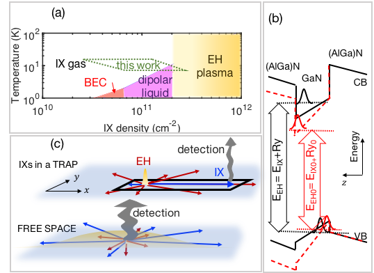
Figure 1: (a) IX phase diagram. Four phases theoretically expected are shown by different colors. The green region delimited by dotted line represents the phase space area explored in this work. The critical density corresponding to the transition towards plasma states is determined in this work. (b) Sketch of the the GaN/(Al,Ga)N QW bands in the absence (red dashed line) and in the presence of optical excitation (black solid line). Corresponding electron and hole wavefunctions and energy levels are shown with the same color code. The band-to-band transitions are indicated by arrows. (c) Artist view of the two ways to study IX emission: ”IX in a trap” (upper sketch) - point-like excitation followed by spatially separated PL analysis in the trap (used in Chiaruttini et al. (2019)) and ”free space” (lower sketch) - broad excitation followed by detection in the center of the excitation spot (used in this work).

The objective of this work is to address the Mott transition of IXs hosted by wide polar GaN/(AlGa)N quantum wells. GaN-hosted IXs have relatively high binding energies ($20$ meV), small Bohr radii ($5$ nm) and greater mass $M=1.6\,m_{0}$, as compared to GaAs-based structures ($m_{0}$ is the free electron mass) Gil (2014). Hence the density/temperature phase diagram (Fig. 1 (a)) is quite different from that of GaAs-based systems.

Because GaN QWs grown along the (0001) crystal axis naturally exhibit built-in electric fields of the order of megavolts per centimeter, IXs are naturally created in the absence of any external electric field Bernardini and Fiorentini (1998); Leroux et al. (1998); Grandjean et al. (1999). This offers the opportunity not only for all-optical generation of IXs, but also for shaping at will the in-plane potential experienced by the IXs by simple deposition of metallic layers on the surface, without application of any external electric bias. We have recently demonstrated the electrostatic trapping and control of the cold IX density in such structures Chiaruttini et al. (2019). IXs at quasi-thermal equilibrium state could be studied in spatial regions situated tens of micrometers away from the laser excitation spot. We called such areas ”excitonic lakes”. We have determined the lower limit for the carrier density for the set of excitation powers used and demonstrated that the carrier temperature remains power-independent. However, despite careful analysis of the spectral shape of the photoluminescence (PL) from the lakes, we could not evidence the onset of the Mott transition.

The reasons for that are numerous. First, the PL lineshape does not show any characteristic shape modification when the system undergoes Mott transition Kash et al. (1991). Second, excitonic correlations, when they are strong, strongly affect the exciton density estimated by comparing the PL energy shift to the one calculated by solving the coupled Schrödinger and Poisson equations (see Fig. A.7) Schindler and Zimmermann (2008); Laikhtman and Rapaport (2009b); Schinner et al. (2013); Cohen et al. (2016); Mazuz-Harpaz et al. (2017). Such correlations can arise from the strong depletion of the exciton gas around a given exciton due to repulsive interactions between IXs. At high IX density they are also expected to favor the transition from an excitonic gas to a dipolar liquid, rather than a Bose-Einstein-like state, see Fig. 1 (a). Third, the IX binding energy at the lowest excitation densities, and the typical blue shift of the electron-hole recombination energy at highest excitation densities are of the same order of magnitude, $\approx 20$ meV. This makes it extremely challenging to unravel the effects of the binding energy reduction, due to the screening of the built-in electric field and exciton-exciton interactions at non-zero density. The density-induced modifications of the QW band diagram and the resulting transition energy shift $E_{int}$ are schematically shown in Fig. 1 (b). Finally, the contribution of the band-to-band emission (unbound electron-hole pairs) to the PL spectrum, that could help us estimating the IX binding energy at least at the lowest excitation densities Deveaud et al. (2005); Kappei et al. (2005); Kiršanskė et al. (2016) is useless in the trap geometry with point-like excitation which we have employed in Chiaruttini et al. (2019). Indeed, when PL is recorded from the same spatial region where the excitation takes place, according to the Saha equation, a mass-action law describing the equilibrium concentration of a gas of coexisting excitons and free carriers, one can eventually extract both exciton and band-to-band emission Zimmermann (1987). This is not the case for a point-like excitation of IXs. Because IXs are rapidly expelled from the excitation spot by strong dipole-dipole interaction, the equilibrium between IXs and band carriers is probably never achieved under the excitation spot (Fig. 1 (c), upper sketch). The detection of the thermalized IXs trapped in the lake tens of micrometers away from the excitation spot does not offer the opportunity to detect simultaneously thermalized IX and band-to-band emission.

In this work we choose a different strategy, based on two key ingredients: (i) broad ($\approx 300$ $\mu$m) and spatially homogeneous excitation, PL detection with spatial resolution, in order to selectively address the emission in the center of the excitation area (Fig. 1 (c), lower sketch). A similar approach has been used in Kappei et al. (2005). The underlying idea is to detect the PL of IXs and free electron-hole pairs coexisting spatially, and to monitor their relative energies and intensities as a function of power and temperature; (ii) application of a magnetic field in Faraday geometry (parallel to the growth axis) in order to discriminate between the diamagnetic field dependence typical of excitons (quadratic energy shift ), from the Landau quantization expected for unbound charge carriers (linear increase of energy, usually referred to as cyclotron shift).

The analysis of the experimental results suggests that at the lowest studied sample temperature ($7$ K) and at the highest excitation power, the carrier density $n\approx 2\times 10^{11}$ cm^-2 and the system undergoes the Mott transition: the zero-field PL energy spectrally merges with the electron-hole emission and the magnetic field dependence changes frrom quadratic to linear. Such a high carrier density could not be reached at $T>7$ K, presumably due to more efficient nonradiative recombination. The determination of the corresponding carrier density is quite complex, because of the interplay between different density-dependent effects: the built-in electrostatic potential, reduction of the exciton binding energy (accompanied by the increase of the in-plane Bohr radius) and build-up of excitonic correlations. In this work, we have tried to unravel their respective contributions. We have also observed that, in contrast to GaAs/(AlGa)As systems, where the transport of dipolar magnetoexcitons is strongly quenched by the magnetic field due to exciton mass enhancement Kuznetsova et al. (2017); Dorow et al. (2017), in GaN/(Al,Ga)N the band parameters are such that the transport is preserved up to $9$ T.

The paper is organised as follows. In the next Section we present the sample and experimental setup. The third Section presents the ensemble of the experimental results, namely the PL study of IX transport as a function of the magnetic field, laser excitation power and temperature. In Section IV we interpret the results in terms of the situation of our experiments in the IX phase diagram. The last section summarises the results and concludes the study.

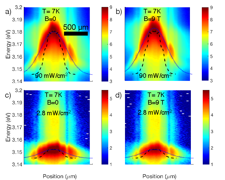
Figure 2: PL intensities (color-encoded in log scale) measured at $T=7$ K and two different excitation power densities: $P=90$ mW/cm² (a,b), $P=2.8$ mW/cm² (c,d), and two magnetic field values: $B=0$ (a,c), $B=9$ T (b,d). The measured laser intensity profile (normlized to unity) is shown by dashed lines. Dotted lines are Gaussian-shaped guides for the eye showing the decrease of the IX emission energy when the distance from the excitation center increases.

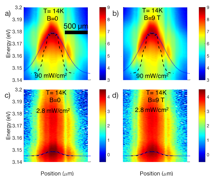
Figure 3: PL intensities (color-encoded in log scale) measured at $T=14$ K and two different excitation power densities: $P=90$ mW/cm² (a,b), $P=2.8$ mW/cm² (c,d), and two magnetic field values: $B=0$ (a,c), $B=9$ T (b,d). The measured laser intensity profile (normalized to unity) is shown by dashed lines. Dotted lines are Gaussian-shaped guides for the eye showing the decrease of the IX emission energy when the distance from the excitation center increases.

II Sample and experimental setup

We investigate a $7.8$ nm-wide GaN QW sandwiched between $50$ (top) and $100$ nm-wide (bottom) Al_0.11Ga_0.89N barriers, grown on a free-standing GaN substrate. The band diagram of such structure is shown schematically in Fig.1 (b). In the absence of photoexcitation the built-in electric field due to spontaneous and piezoelectric polarization confines electrons and holes at the two opposite interfaces of the QW. In the studied structure the field effect is so strong that the ground state exciton energy ($E_{IX0}=3.145$ eV in Fig. 1 (b)) is pushed below the exciton energy in bulk GaN $E_{GaN}=3.49$ eV Bernardini and Fiorentini (1998); Leroux et al. (1998); Grandjean et al. (1999, 2000); Gil (2014); Chiaruttini et al. (2019). The corresponding IX radiative lifetime is estimated as $\tau_{0}\approx 10$ $\mu$s, orders of magnitude longer than in traditional narrow QWs Lefebvre et al. (1999); Fedichkin et al. (2015); Rosales et al. (2013); Rossbach et al. (2014). The sample is placed in a variable temperature magneto-optical cryostat and cooled down to temperatures in the range from $T=7$ to $14$ K. Magnetic fields $B$ up to $9$ T created by superconducting magnets are applied in the Faraday geometry (parallel to the QW growth axis). We use a continuous wave laser excitation at $\lambda=355$ nm, very close to the GaN bandgap energy, but well below the emission energy of the Al_0.11Ga_0.89N barriers. The laser beam is loosely focused on the sample surface ($\approx 300$ $\mu$m-diameter spot) in order to create a broad, homogeneously excited area (see dashed lines in Figs. 2 and 3). The PL spectra are acquired by a charge coupled device (CCD) camera over $1.5$ mm with $\approx 25$ $\mu$m spatial resolution (pixel size). Such broad excitation combined with the spatially resolved detection appeared to be critically important to address the question of the Mott transition. As anticipated in the introduction and as we explain in more details in the next Section, this allows us to detect the PL from IXs and from unbound electron-hole pairs that coexist spatially, and thus to monitor the reduction of the IX binding energy. This also gives us access to carrier transport properties, so that we can directly verify the assumptions regarding transport in our modelling. More details on the sample parameters and on the setup are given in the Appendix.

III Experimental results and discussion

III.1 Exciton transport

The exciton transport at $T=7$ K and $T=14$ K is presented in Figs. 2 and 3, respectively. They show color-encoded PL spectra, measured at various distances from the excitation spot for two different power densities, and at two values of the magnetic field, $B=0$ and $9$ T. Excitation spot intensity profile is shown by the dashed lines. The blue dotted lines are guides for the eye, helping to visualise the IX emission peak energy as a function of the distance from the spot center.

Let us first concentrate on the $B=0$ transport. Clearly, the energy of the excitonic PL decreases when moving away from the excitation spot center, similarly to the case of the point-like excitation Fedichkin et al. (2016, 2015); Chiaruttini et al. (2019). Such decrease of the emission energy and intensity indicates that the exciton density decreases. The relation between PL energy and IX density is particularly strong in wide QWs due to interactions between IXs that have large dipole moment, and the resulting screening of the electric field along the growth direction: the highest density under the pumping spot corresponds to the maximum screening (lowest electric field), and thus to the highest emission intensity and energy Lefebvre et al. (2004); Fedichkin et al. (2016, 2015); Chiaruttini et al. (2019). The interaction-induced increase of the IX energy reaches $40$ meV ($10$ meV) at the spot center and at highest (lowest) power densities that we could explore in our experiments. This shift can be used to estimate the IX density as $n=E_{int}/\phi_{0}$, where $\phi_{0}=1.5\times 10^{-13}$ eV$\cdot$cm^-2 is the coefficient extracted from the self-consistent solution of the Schrödinger and Poisson equations (plate capacitor-like model) Lefebvre et al. (2004); Fedichkin et al. (2016, 2015); Chiaruttini et al. (2019). This estimate needs to be improved by taking into account the exciton binding energy (which decreases when the IX density increases) and excitonic correlations, which become signicant at low temperatures and high densities. As we will discuss later on (see also Figs. 6, A.7), both of these effects may substantially alter our estimation of the IX density needed to induce a given blue shift  Schindler and Zimmermann (2008); Laikhtman and Rapaport (2009b, a).

From the $B=0$ emission profiles measured at highest power density $P=90$ mW/cm² we deduce that despite spatially broad excitation as compared to previous experiments involving point-like excitation, IX transport is still clearly observable both at $7$ K and $14$ K Fedichkin et al. (2016, 2015); Chiaruttini et al. (2019). The full width at half maximum (FWHM) of the emission pattern is approximately $800$ $\mu$m. By contrast, for the lowest power density $P=2.8$ mW/cm² the IX transport is only apparent at $T=7$ K (same FWHM as at high power), while at $T=14$ K the emission profile coincides with the excitation one. The quenching of the IX transport with decreasing power observed at $T=14$ K is a usually observed and well understood phenomenon Remeika et al. (2009); Leonard et al. (2012); Rapaport et al. (2006); Fedichkin et al. (2015). Modelling IX transport by drift-diffusion equation shows that this is due to weaker dipole-dipole repulsion, that depends on the density. More efficient localization on the QW interfaces at low IX densities may also hinder the transport Ivanov (2002); Remeika et al. (2009); Leonard et al. (2012); Rapaport et al. (2006); Fedichkin et al. (2016, 2015). By contrast, the persistence of the transport at $7$ K is rather surprising, especially because carrier localization is expected to be enhanced at lower temperatures.

The effect of the magnetic field up to $9$ T on the IX transport appears to be very weak. From the color-encoded spectra in Figs. 2 and 3 one can see that the FWHM of the emission pattern does not change. This behaviour differs significantly from that of IXs in GaAs/(Al,Ga)As coupled QWs, where magnetic field of the similar strengths has been shown to strongly inhibits IX transport. Kuznetsova et al. (2017); Dorow et al. (2017). This is due to the fact that IXs hosted by GaAs/(Al,Ga)As coupled QWs are much lighter particles, with much wider radii. Therefore, the ratio $\chi$ between cyclotron energy $\hbar\omega_{c}$ and exciton binding energy $Ry$, $\chi=\hbar\omega_{c}/2Ry$ increases much faster with magnetic field. When magnetic energy dominates over the electron-hole Coulomb interaction, $\chi\gg 1$, the system is described in terms of so-called magnetoexciton Lozovik and Ruvinskii (1997); Butov et al. (2001); Lozovik et al. (2002). The magnetic field leads in this case to the strong reduction of the in-plane Bohr radius $a_{B}$ and enhancement of the in-plane exciton mass $M$Edelstein et al. (1989); Lozovik et al. (2002); Butov et al. (2001); Stépnicki et al. (2015); Arnardottir et al. (2012); Wilkes and Muljarov (2017, 2016); Kuznetsova et al. (2017); Dorow et al. (2017). Therefore, the reduction of the diffusion coefficient $D=l\sqrt{2k_{B}T/M}$ and the mobility $\mu_{X}=D/k_{B}T$ is observed Kuznetsova et al. (2017); Dorow et al. (2017). Here $l$ is the exciton scattering length and $k_{B}$ is the Boltzmann constant. In GaN/(Al,Ga)N structures studied in this work and up to $9$ T we seem to deal with the opposite limit: $\chi\ll 1$. Numerical modelling of the IX transport within drift-diffusion model (see Appendix) Fedichkin et al. (2015); Chiaruttini et al. (2019) allows us to estimate that the enhancement of the exciton mass $M(B)/M$ does not exceed a few percents at $B<9$ T, in consistance with estimations that can be done in the $\chi<1$ regime Arseev and Dzyubenko (1998); Wilkes and Muljarov (2016) :

$$M(B)/M=(1-42\mu(a_{B}/l_{B})^{4}/16^{2}M)^{-1}.$$ (1)

Here $l_{B}=\sqrt{\hbar/eB}$ is the magnetic length, $e$ is the electron charge, $\hbar$ is the reduced Planck constant, $\mu$ is the exciton in-plane reduced mass. Thus, in the following we assume that the shift of the IX emission energy measured at the center of the exciton spot in the presence of the magnetic field is entirely local, that is not affected by the in-plane transport, in contrast to the case of IXs in GaAs/(Al,Ga)As QWs.

III.2 Magnetic field-induced exciton energy shift

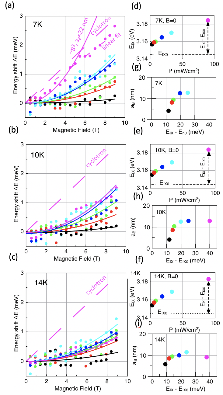
Figure 4: (a-c) IX emission energy shift with respect to the $B=0$ emission energy as a function of the magnetic field at $T=7$ K (a), $T=10$ K (b), $T=14$ K (c) for various excitation power densities from $P=2.8$ mW/cm² (black symbols) to $P=90$ mW/cm² (magenta symbols). Solid lines are parabolic fits to the diamagnetic shift model. The model does not fit the highest power data in (a), and the linear fit is shown by the long-dash line. Short-dash line in (a) shows the cyclotron shift expected for unbound electron-hole pairs. (d-f) show the emission energy at $B=0$ for each power density and three different temperatures. The horizontal dashed line shows zero-density limit $E_{\mathrm{IX0}}$ of the exciton emission energy. The vertical dashed arrow illustrates the density-induced blue shift of the emission line at $P=90$ mW/cm². (g-i) Values of Bohr radius extracted from the quadratic fit (a-c) as a function of the zero-field density-induced energy shift. Excitation power density is shown with the same colour code in (a-c), (d-f) and (g-i).

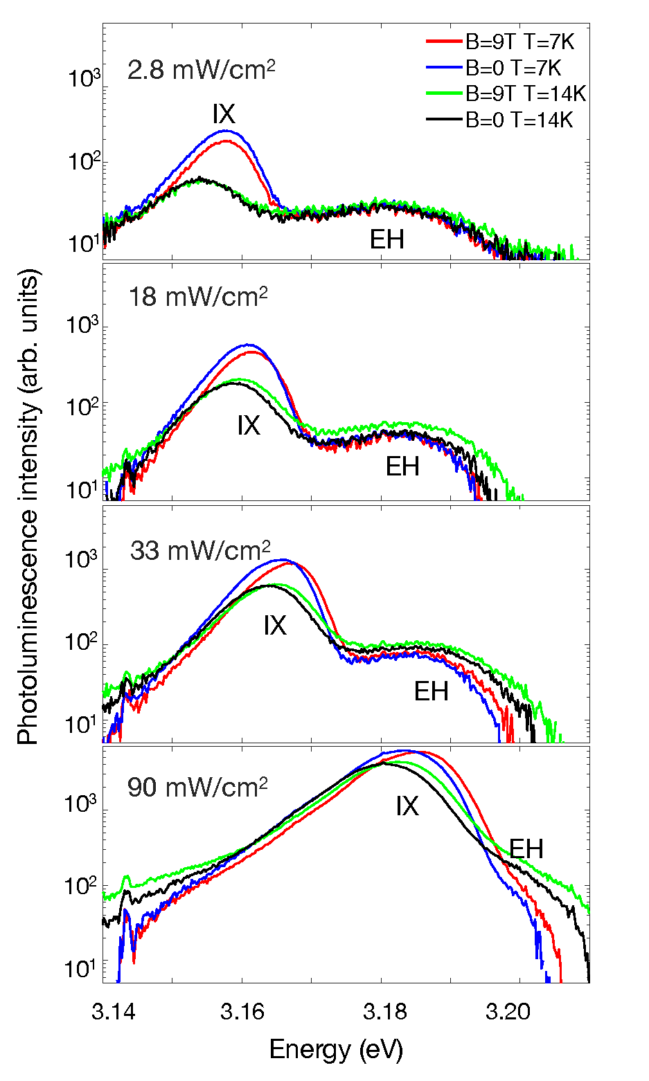
Figure 5: PL spectra collected from $25$ $\mu$m-diameter area in the center of the excitation spot at different power densities. Two temperatures ($T=7$ K, $T=14$ K) and two magnetic field values ($B=0$ and $B=9$ T) are shown for each power. We identify the two emission lines as IXs and unbound electron-hole pairs (EH).

The shift of the IX emission energy peak with respect to $B=0$ (averaged over $\approx 25$ $\mu$m) measured as a function of the magnetic field at different excitation power densities is shown by symbols in Fig. 4 for $T=7$ K (a), $T=10$ K (b), and $T=14$ K (c). Panels (d-f) indicate for each temperature the correspondence between the emission energy $E_{\mathrm{IX}}$ measured at $B=0$ and the power density. The colour code is the same as in (a-c). The energies used to extract these shifts are obtained by the spectrum fitting procedure described in Appendix A4. One can see that at maximum field $B=9$ T the energy shift varies in the range from $0.2$ to $3$ meV. The largest shifts are achieved at highest powers and lowest temperatures. Except for the highest power at $7$ K, the IX energy shifts quadratically with the magnetic field. This can be interpreted as a diamagnetic shift $\Delta E=\gamma_{D}B^{2}$, where $\gamma_{D}=e^{2}a_{B}^{2}/(8\mu)$ is the so-called diamagnetic coefficient Bugajski et al. (1986). The diamagnetic coefficient appears to increase with the excitation power, suggesting that IX Bohr radius increases as well. This is a signature of the progressive screening of the electron-hole Coulomb interaction within each IX. The reduced exciton mass in GaN being well known ($\mu=0.18m_{0}$), fitting of the data to the quadratic dependence (solid lines in Fig. 4) allows us to extract the values of Bohr radii for all excitation power densities and temperatures.

The ensemble of the resulting values of $a_{B}$ are presented in Fig. 4 (g-i). One can see that the Bohr radius can be as small as $5-6$ nm. Note, that relatively small values of Bohr radius (compared to the prediction of the self-consistent variational calculation of $a_{B}$ Bigenwald et al. (1999, )) are consistent with large exciton binding energy that we deduce from the PL spectra, where both exciton and free carrier emission are observed (see Fig. 5). This will be further discussed in Sec. III.3.

For each value of the sample temperature, the values of $a_{B}$ are shown as a function of the emission energy shift $E_{IX}-E_{IX0}$ at $B=0$. This shift is related to the IX density in the QW and contains two contributions with different signs. The first one is the blue shift due to the interaction energy, and the second one is the red shift due to exciton binding energy (see Fig. 1). Their relative contribution will be discussed in Sec. IV.1.

Let us now consider the set of measurements at $T=7$ K in Fig. 4 (a) that corresponds to the highest excitation power $P=90$ mW/cm² (magenta circles). In contrast with other measurements the energy shift does not grow quadratically with magnetic field. For comparison solid magenta line in Fig. 4 (a) corresponds to $a_{B}=22$ nm, much larger than $a_{B}\approx 12$ nm at higher temperatures and maximum powers. Instead, the data are much better described by a linear function $\Delta E=\gamma_{L}B$, with the slope $\gamma_{L}=0.27$ meV/T . Remarkably, the slope obtained from the linear fit is very close to $\gamma_{c}=e\hbar/(2\mu)=0.32$ meV/T, that one could expect for the cyclotron energy of the electron-hole pair. This suggests that, indeed, the density of the electron-hole pairs in the QW plane is high enough to screen the Coulomb interaction within IX, so that the Mott transition could be reached.

The reason why this transition could only be observed at $7$ K needs to be elucidated. In particular, it is important to find out wether this is due to the higher density reached in this case (e.g. due to different nonradiative losses), or due to the screening of the exciton binding, that would be more efficient at low temperature. Below we try to answer this question and to determine $n_{\mathrm{Mott}}$, the critical density at the Mott transition. We recall that the analysis made in this work is based on the assumption that the magnetic field up to $9$ T (that induces a cyclotron shift of the electron-hole pair emission $\hbar\omega_{c}/2=3$ meV ) can be considered as a small perturbation with respect to the exciton binding energy, i.e. $Ry\gg\hbar\omega_{c}/2$. Therefore the formation of magnetoexciton does not take place. This differs from the GaAs-based structures where the transition from Coulomb-bound exciton to magnetoexciton has been reported to occur at lower magnetic fields $\approx 2$ T Butov et al. (1999).

III.3 Photoluminescence of excitons vs free arriers

Let us consider in detail the PL spectra collected from the $25$ $\mu$m-diameter area in the center of the excitation spot at different power densities and temperatures (Fig. 5). For the lowest excitation density (solid lines) we identify two emission lines, separated by $\approx 25$ meV, the lowest energy line is the one that we have identified as the IX emission. It has higher intensity and it is shifted towards higher energy by the magnetic field (as shown in Fig. 4), while the second line is so wide, that it is difficult to quantify the energy shift induced by the magnetic field. When the excitation power increases, the IX emission strongly shifts towards higher energies up to merging with the higher energy emission line, which shifts much less. Note also that the ratio between the intensities of the IX and the high energy line is $\approx 5$ times higher at $T=7$ K than at $T=14$ K.

We tentatively interpret the higher energy line as an emission of the unbound electron-hole (EH) pairs, that coexists with IXs even at the lowest excitation densities explored in this work. This contribution is not negligible as compared to the lower energy IX, because the corresponding density of states is huge. EH emission can be spectrally separated from IX, because the linewidth of IX emission is smaller than IX binding energy. Similar PL behavior has already been observed in both GaAs and InGaAs QWs Deveaud et al. (2005); Kappei et al. (2005); Kiršanskė et al. (2016). In GaN-based heterostructures the efficient formation of excitons even within a dense electron-hole plasma has already been observed by time-resolved terahertz spectroscopy Hangleiter et al. (2015). Both energy and intensity of the EH emission with respect to the well-identified IX emission are consistent with this interpretation: IX line merges with the EH plasma at high density, and the ratio between IX and EH intensity decreases when the temperature increases. The power-induced shift of the IX line is larger than that of the EH line. This is because EH transition energy is affected only by the screening of the built-in electrostatic potential, while IXs experience both this screening and the reduction of the binding energy. Note also, that the EH emission line is much broader ($30$ meV at the lowest power, compared to $10$ meV for IXs) and weaker ($\approx 5$ times for the lowest power density) than the IX line. That is why it was not possible to quantify the magnetic field-induced shift of the EH line, that is expected to be smaller than $3$ meV at highest accessible magnetic field.

The simultaneous observation of EH and IX emission provides us with some important information. Indeed, the energy splitting between IX and EH lines characterises the exciton binding energy $Ry$, which, due to many-body effects, depends on the density of the particles in the QW Zimmermann (1987). From the measurements at the lowest power we estimate $Ry_{0}=25$ meV, corresponding to the zero-density limit. Exciton binding energy is related to its Bohr radius $Ry=e^{2}/4\pi\varepsilon a_{B}$, where $\varepsilon$ is dielectric permittivity constant in the hosting semiconductor (here GaN). This yields $a_{B0}=6$ nm in the zero-density limit. As already mentioned in the Sec. III.2, these values are not properly described by the self-consistent variational calculation of the excitonic properties Bigenwald et al. (1999, 2000, ). The relevance of this model relies on the choice of the variational function, and so far has not been verified experimentally. Moreover, the model predicts that IX binding energy and Bohr radius remain constant up to approximately $10^{11}$ cm^-2 pair density (corresponding to emission energy shift $>10$ meV), which also contradicts our experiments. Thus, in what follows we rely on the experiments and use the value of $Ry_{0}=25$ meV and its relation to $a_{B}$ in order to estimate the exciton density as a function of power and temperature and determine the Mott density.

IV Discussion

IV.1 Determination of the exciton densities

Estimation of the exciton densities and the critical densities for exciton dissociation is an extremely delicate task, even in the case of traditional excitons with zero dipole moment. In particular, quantifying exchange and correlations within excitonic ensembles is a complex many-body problem. For IXs, density-dependent screening of the built-in electric field is another complicating factor, because it might be difficult to separate it from exciton-exciton interaction. We describe below the procedure that we adopted here to estimate power and temperature dependent exciton densities, Bohr radii and binding energies within available models.

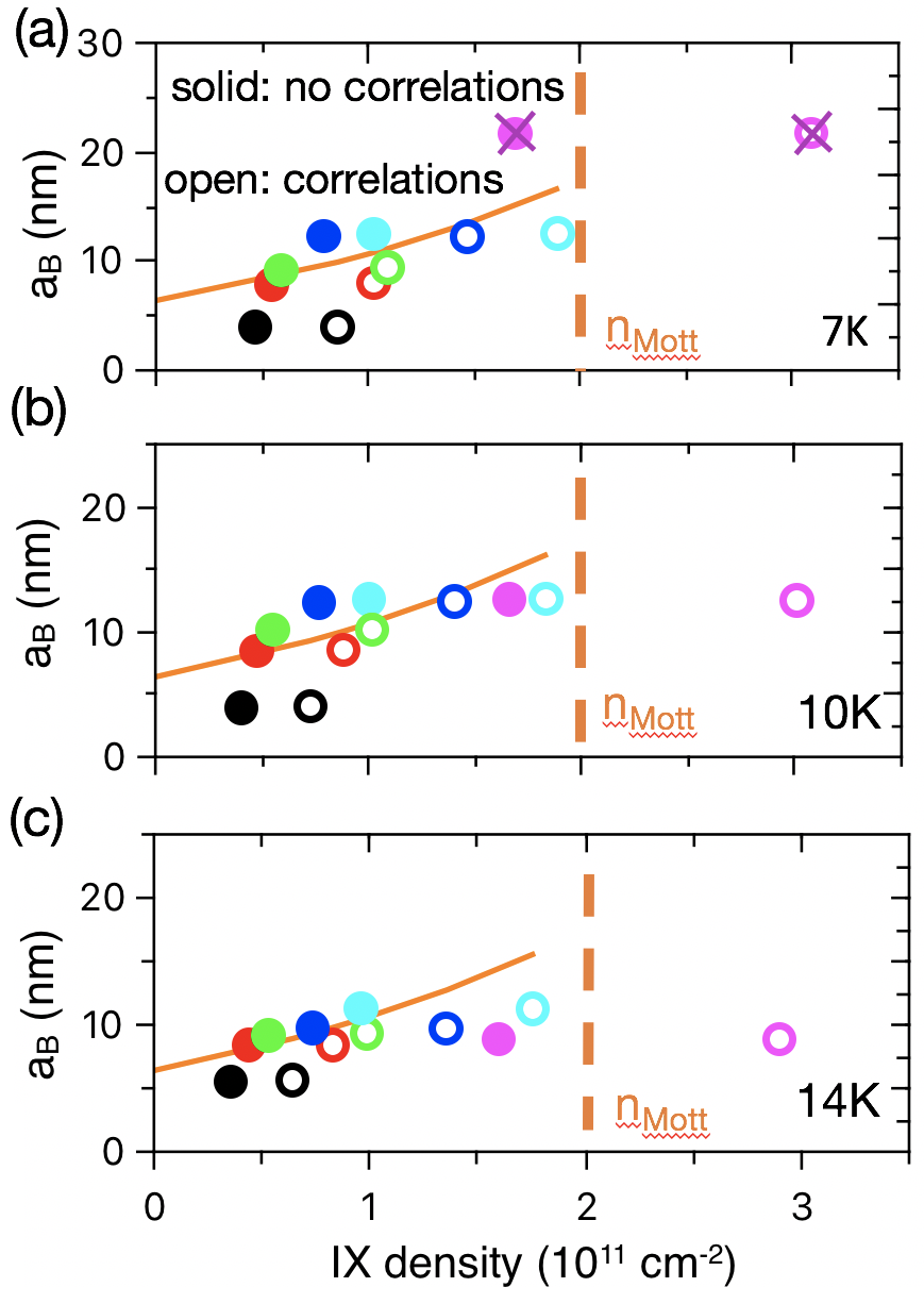
Figure 6: Exciton Bohr radius (solid lines) as a function of the IX density calculated within exponential model assuming $n_{\mathrm{Mott}}=2\times 10^{11}$ cm^-2 (dashed lines) and $Ry_{0}=25$ meV. These assumptions are identical for the three different temperatures (a-c). Symbols show the Bohr radii extracted from the diamagnetic shift at different powers (same as in Fig. 4, same color code) as a function of the carrier density calculated from the corresponding emission energy at $B=0$. Open (filled) symbols show the calculation within Model C (Model NC). At $7$ K crosses on top of the circles indicate the density points where magnetic field-induced energy shift is linear, so that the interpretation in terms of the diamagnetic shift is not satisfactory (the emission is expected to be dominated by the electron-hole plasma).

The analysis is based on three experimentally determined (or deduced from them) parameters: (i) the value of the zero-density binding energy $Ry_{0}=25$ meV estimated from the spectral splitting between IX and EH emission lines at the lowest density; (ii) the corresponding zero-density Bohr radius $a_{B0}=6$ nm; (iii) zero-density IX emission energy $E_{\mathrm{IX0}}=3.145$ meV, measured $\approx 700$ $\mu$m away from the excitation spot (see e.g. Figs. 2-3 (c). These values are identical for all temperatures, within the accessible precision.

We start from the calculation of the electron-hole pair density corresponding to a given band-to-band transition energy

$$E_{\mathrm{{EH}}}(n)=E_{\mathrm{{EH0}}}+E_{\mathrm{{int}}}(n)$$ (2)

using self-consistent solution of the coupled Schrödinger and Poisson equations (see Appendix A5.1). The result of such calculation is very well approximated by the plate capacitor-like model, where density-induced blue shift is given by $E_{\mathrm{{int}}}=\phi_{0}n$, with $\phi_{0}=1.5\times 10^{-13}$ eV cm^-2. Here $E_{\mathrm{EH0}}$ is the zero-density band-to-band transition energy, that does not yet account for the exciton binding energy $E_{\mathrm{{EH0}}}=E_{\mathrm{{IX0}}}+Ry_{0}=3.17$ eV.

As already mentioned, this approach completely neglects the correlation effects which, at sufficiently high density and low temperature, result in strong enhancement of the exciton density expected at a given PL energy shift Schindler and Zimmermann (2008); Laikhtman and Rapaport (2009b). We try to include these correlation effects in our model and calculate $E_{\mathrm{int}}$ using a more sophisticated approach Schindler and Zimmermann (2008). Thus, we have two ways to calculate the band-to-band transition energy $E_{\mathrm{EH}}$, either including (Model C), or not including (Model NC) exciton correlation effects. The details of these calculations are reported in the Appendix (Secs. A5.2 and A5.1).

Because in our system $E_{\mathrm{int}}$ can reach values of the same order as $Ry_{0}$, that is $\approx 10-20$ meV, it is important to take into account the variations of binding energy when the IX density is increased:

$$E_{\mathrm{IX}}(n)=E_{\mathrm{EH}}(n)-Ry(n).$$ (3)

The simplest exponential model is chosen to account for the density-induced reduction of the exciton binding energy due to many-body effects:

$$Ry(n)=Ry_{0}\times\mathrm{exp}(-n/n_{\mathrm{Mott}}),$$ (4)

where $n_{\mathrm{Mott}}$ is a free parameter Liu et al. (2016). The corresponding Bohr radius $a_{B}(n)$ is calculated from $Ry(n)$ as :

$$a_{B}(n)=a_{B0}\times Ry(n)/Ry_{0}.$$ (5)

Eqs. 2 - 5 can be solved for any value of the fitting parameter $n_{\mathrm{Mott}}$. This allows us to establish the relation between IX Bohr radius and particle density, either including (Model C) or not (Model NC) the excitonic correlations, for each value of the excitation power and temperature. The value $n_{\mathrm{Mott}}=(2\pm 0.5)\times 10^{11}$ cm^-2 ensures the best fit between the values of $a_{B}$ calculated from Eq. 5 and those extracted from magnetic field-induced diamagnetic shift.

The results of this analysis are summarized in Fig. 6 for three different temperatures. The correspondence between IX density and Bohr radius calculated within Model C (open symbols) and Model NC (filled symbols) is shown for all excitation powers. At $7$ K crosses on top of the circles indicate the highest density point ($P=90$ W/cm²), where the energy shift induced by magnetic field is linear, so that the interpretation in terms of diamagnetic shift is not satisfactory. Lines indicate the model assumption for $a_{B}(n)$ given by Eq.5 (solid line) and Mott density resulting from the best fit to the data (dashed line).

One can see that within the relevant density/temperature parameter range the difference in the density estimation between two models does not exceed a factor of two. At all powers except the highest one (magenta symbols), both models describe the experimental data reasonably well. Namely, exciton density remains below $n_{\mathrm{Mott}}$, consistent with the experimentally observed diamagnetic behaviour. By contrast, at $P=90$ mW/cm² only Model C allows us to describe the Mott transition observed at $T=7$ K. Nevertheless, despite the temperature dependence that it intrinsically includes (see Appendix), Model C fails to describe the absence of Mott transition at $T=10$ and $14$ K. It seems to overestimate the role of the correlations at $T>10$ K, while simpler Model NC provides better agreement with the data. Thus, none of the models fits to the ensemble of the data. In the attempt to reconstruct the IX phase diagram shown in Fig. 1, we assume that the densities are given by Model C at $T=7$ K and by Model NC at higher temperatures.

IV.2 IX phase diagram

The determination of the exciton densities and the Mott transition (only reached at $T=7$ K) allows us to draw the parameter space explored in this work on the theoretical IX phase diagram presented in Fig. 1 (a). The critical temperature for the formation of the BEC-like state is given by $k_{B}T_{\mathrm{{BEC}}}=2\pi\hbar^{2}n/M$ (red area), and for the formation of the correlated dipolar liquid $k_{B}T_{\mathrm{{DL}}}=(4\pi\varepsilon n/(ed)^{2})^{2/3}$ (magenta area) Laikhtman and Rapaport (2009b); Butov (2016); Combescot et al. (2017). Here $\varepsilon$ is the dielectric constant in the matter (GaN). The exciton parameter space explored here (grey area) is expected to span over three different phases: gas, dipolar liquid and electron-hole plasma.

The Mott transition from excitons to ionised electron-hole pairs at $n_{\mathrm{Mott}}\approx 2\times 10^{11}$ cm^-2 has only been observed at $7$ K, because only at this lowest explored temperature such high density could be reached. Indeed, the experimental configuration that we used relies on broad excitation, that limits accessible laser power density. Some non-radiative losses could be sufficient to reduce the carrier density by a factor of the order of two, making the transition inaccessible. Since we have no experimental determination of the temperature dependence of the Mott density, it is represented in Fig. 1 (a) as a temperature-independent phase boundary. Note that in narrow GaN/(Al,Ga)N QWs hosting excitons such that their dipolar moment is negligibly small and $n_{\mathrm{Mott}}$ is three times higher than in our structure, no temperature dependence of the Mott density have been found up to $150$ K Rossbach et al. (2014). The estimated value of $n_{\mathrm{Mott}}$ is three times lower than the one reported in similar structures but with narrow QWs, and thus non-dipolar excitons Rossbach et al. (2014).

The interpretation of the Mott transition observed at $7$ K is complex. Our analysis of the underlying densities as well as the theoretically expected formation of the liquid stated suggests the importance of the excitonic correlations at this temperature. Another indication on the onset of the correlations, is the differences in the excitonic transport at $7$ K and at higher temperatures. As pointed out in Sec. III.1 (Fig. 2), at $7$ K the excitonic drift remains efficient even at the lowest density used in this work. This behaviour is not correctly described by the simple transport model that does fit properly the transport at $14$ K. Note, that the enhancement of the exciton propagation at low temperature exclude the localization effects as a possible cause of the observed effects.

The precision of the procedure used in this work to explore the onset of the many-body effects has of course a number of limitations. In particular, we use an oversimplified relation between exciton Bohr radius and its binding energy and neglect non-radiative effects. Moreover, our considerations neglect possible magnetic field dependence of the exciton Bohr radius and eventual transition towards magnetoexiton states at highest magnetic fields Butov et al. (1999). Although electron-hole binding energy seems to remain higher than the cyclotron energy these effects may affect the results. To confirm and better quantify the onset of many-body effects (dipole-dipole excitonic correlations and Mott transition) future work should focus on (i) lowering down the temperature of the carriers in this system, (ii) comparing the systems hosting IXs with different dipole length. Measurable effects can be expected already at $T=2$ K, and with a $2-3$ nm variation of the QW width.

V Conclusions

In conclusion, using the PL spectroscopy in Faraday configuration we demonstrated the transition from the dipolar IX fluid to the EH plasma in wide polar GaN/(AlGa)N QWs at $7$ K. The corresponding pair density $n_{\mathrm{Mott}}=(2\pm 0.5)\times 10^{11}$ cm^-2 could not be reached at higher temperatures, presumably due to non-radiative losses. We have shown that below Mott transition, IX fluid and unbound EH pairs coexist and can be spectrally separated. The increase of carrier density in the system is accompanied by the screening of both the built-in electric field and the IX binding energy. In the explored parameter range, these two contributions are of the same order. Our modelling suggests the build-up of the exciton-exciton correlations and the possible formation of the dipolar liquid at lowest temperature $T=7$ K. Finally, in contrast with GaAs-hosted IXs, the radial transport of the IXs GaN/(Al,Ga)N QWs appears to be preserved under magnetic field up to $B=9$ T.

Parameter	Units	Value
QW width	(nm)	$7.8$
Al composition in the (Al,Ga)N barriers	(%)	$11$
Al0.11Ga0.89N cap layer thickness	(nm)	50
Al0.11Ga0.89N bottom layer thickness	(nm)	100
GaN buffer layer thickness	(nm)	800
Dislocation density in GaN substrate	(cm-2)	$\sim 2\times 10^{7}$
IX emission energy $E_{IX0}$ at $n\approx 0$	(eV)	$\sim 3.145$
IX binding energy $Ry_{0}$ at $n\approx 0$	(meV)	$\sim 25$
IX radiative lifetime $\tau_{0}$ at $n\approx 0$	($\mu$s)	$\sim 40$
$m^{z}_{e}$ for electron in GaN	($m_{0}$)	$0.200$
$m^{z}_{h}$ for hole in GaN	($m_{0}$)	$1.1$
$m^{z}_{e}$ for electron in Al0.11Ga0.89N	($m_{0}$)	$0.213$
$m^{z}_{h}$ for hole in Al0.11Ga0.89N	($m_{0}$)	$1.367$
$m^{\perp}_{e}$ transverse electron mass in QW	($m_{0}$)	$0.2$
$m^{\perp}_{h}$ transverse hole mass in QW	($m_{0}$)	$1.6$
$\varepsilon$ Dielectric constant in GaN	($\varepsilon_{0}$)	$8.9$
$\varepsilon_{B}$ Dielectric constant in (Al,Ga)N	($\varepsilon_{0}$)	$8.926$
GaN bandgap energy at 7 K	(eV)	$3.507$
(Al,Ga)N bandgap energy at 7 K	(eV)	$3.709$
Band offset in GaN and (Al,Ga)N	(%)	$80$

Table 1: Sample and material parameters used in various calculations Vurgaftman et al. (2001); Vurgaftman and Meyer (2003); Kabi et al. (2009); Rickert et al. (2002).

Parameter	Units	Value
Built-in electric field $F$	(kV/cm)	980
Exciton radiative lifetime factor $\gamma$	(cm-2)	$2.7\times 10^{11}$
IX-IX interaction constant $\phi_{0}$	(eV$\cdot$cm2)	$1.50\times 10^{-13}$
IX Bohr radius $a_{B0}$ at $n\approx 0$	($\mu$m)	$\sim 6$
Band-to-band transition $E_{EH0}$	(eV)	$\sim 3.17$

Table 2: Sample parameters from self-consistent solution of Schrödinger and Poisson equations.

VI Acknowledgments

We are grateful to L. V. Butov for enlightening discussions. This work was supported by the French National Research Agency via OBELIX and IXTASE projects, as well as LABEX GANEX.

VII Appendix

A1 Sample structure

The sample is grown by molecular beam epitaxy (MBE) on a c-plane oriented n-type GaN LUMILOG substrate with $\sim 2\times 10^{7}\mathrm{cm^{-2}}$ threading dislocation density. The substrate is covered by a $0.8$ $\mu$m-thick GaN buffer layer under the active zone. The active zone consists of a $7.8$ nm-wide GaN QW sandwiched between $50$ nm (top) and $100$ nm-wide (bottom) Al_0.11Ga_0.89N barriers. The main characteristics of the sample, material properties used in calculations, and the results of various calculations are summarized in Tables 1-2.

A2 Spatially-resolved PL setup under magnetic field

The sample is placed in the chamber of a variable temperature insert (VTI) of the magneto-optical cryostat (Cryogenic Limited). The magnetic field up to $9$ T is created by superconducting coils in Faraday geometry.

Optical set-up is shown in the Fig. A.1. The laser source is a continuous emission at 355 nm (Coherent OBIS, nominal power 20 mW). The beam is first shaped by an expander (L1, L2) to increase the numerical aperture incident on the objective lens (LO) which focuses the excitation on the sample surface. The diameter of the laser spot thus focused can be reduced upto about 20 µm. We deliberately deregulated the beam expander in order to increase the size of the incident spot on the sample up to 300 $\mu$m.

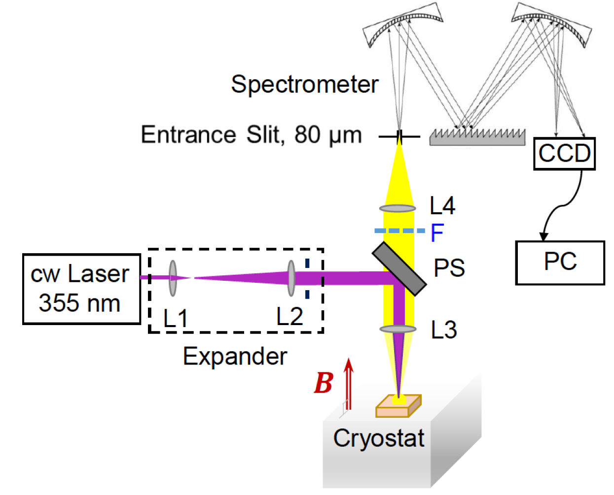
Figure A.1: Experimental set-up.

The luminescence is collected by the same objective lens (L3). A bandpass filter (F, Semrock 400/16 nm) placed behind a power-splitter (PS) eliminates the reflection of the laser beam. The sample is imaged on the spectrometer (Horiba Jobin Yvon iHR550) entrance slit (80 $\mu$m) . The signal is then sent to a CCD  camera: each pixel corresponds to 27 µm on the sample.

A3 Modelling of the IX transport

The model used here is identical to the one that we used in Refs. Fedichkin et al., 2015; Chiaruttini et al., 2019. It is based on the equation for the in-plane transport of indirect excitons. In its most general form reads:Ivanov (2002); Rapaport et al. (2006)

$$\frac{\partial n}{\partial t}=-\nabla\cdot\mathbf{J}+G-Rn,$$ (A1)

where $n$ is the exciton density,

$$G=\frac{N_{p}}{\left(\pi a_{0}^{2}+\pi w^{2}/2\right)}\times\textrm{erfc}\left(\frac{r-a_{0}}{w}\right)$$ (A2)

is the exciton density generation rate, $N_{p}$ is the number of excitons generated per second, $a_{0}$ and $w$ are the laser spot geometric factors, $R$ is the recombination rate, $\mathbf{J}$ is the IX current density. In order to describe the spatial profile of the spot we have chosen the parameters in Eq. A2 as $w=100$ $\mu$m, $a_{0}=200$ $\mu$m. The exciton current $\mathbf{J}$ can be split into drift and diffusion components: $\mathbf{J}=\mathbf{J}_{\mathrm{drift}}+\mathbf{J}_{\mathrm{diff}}$.

The diffusion current $\mathbf{J}_{\mathrm{diff}}$ is given by:

$$\mathbf{J}_{\mathrm{diff}}=-D\nabla n$$ (A3)

where $D$ is the exciton diffusion coefficient $D=l\sqrt{2k_{B}T/M}$. It depends on the exciton scattering length $l$ Rapaport et al. (2006); Fedichkin et al. (2015), but also on the exciton in-plane mass $M=m^{\perp}_{e}+m^{\perp}_{h}$ that can be affected by the magnetic field: $M(B)/M=1+\delta M$. The drift term $\mathbf{J}_{\mathrm{drift}}$ in Eq. A1 can be rewritten as

$$\mathbf{J}_{\mathrm{drift}}=-\mu_{X}n\nabla(\phi_{0}n)$$ (A4)

where the exciton mobility $\mu_{X}$ is connected to the diffusion coefficient $D$ via the Einstein relation: $\mu_{X}=D/k_{B}T$. In Eq. A4, the drift is governed by the exciton-exciton interaction energy $\phi_{0}n$ only. The recombination rate $R$ is assumed to be dominated by radiative mechanisms $R=1/\tau_{rad}$, where density dependent radiative recombination time is given by $\tau_{rad}=\tau_{0}\exp(-n/\gamma)$ and $\gamma$ is obtained from the the solution of the coupled Schrödinger and Poisson equations Lefebvre et al. (2004); Fedichkin et al. (2015); Chiaruttini et al. (2019) and $\tau_{0}=40$ ms (see Table 2 ).

We look for the steady-state solutions $n(r)$ of Eq. (A1) at $T=14$ K in order to evaluate the eventual effect of the IX mass enhancement on the in-plane transport. The emission profiles measured experimentally are compared with the calculated spatial profiles of (i) the exciton emission energy shift $\Phi_{0}n$ and (ii) the exciton PL intensity $I=nR$ at two different power densities, the lowest and the highest ones. The corresponding values of $N_{P}$ in Eq. A2 are $N_{P}=1.2\times 10^{12}$ s^-1 for $P=2.8$ mW/cm² and $N_{P}=40\times 10^{12}$ s^-1 for $P=90$ mW/cm².

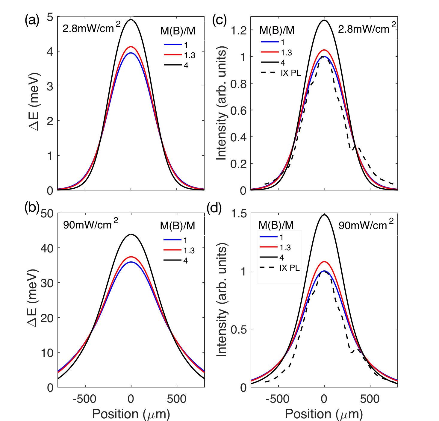
Figure A.2: Calculated spatial distribution of the emission energy shift (a-b) and the intensity (c-d) for three different values $M(B)/M$ and two power densities. Dashed lines in (c-d) show measured IX intensity at $T=14$ K (there is no difference in the $B=0$ and $B=9$ T profiles).

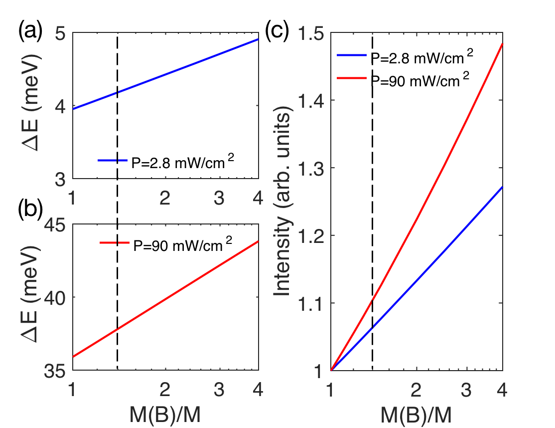
Figure A.3: Energy shift (a-b) and intensity increase (c) in the center of the excitation spot calculated as a function of $M(B)/M$ for two different values of power density. Dashed lines point the value $M(B)/M=1.3$, the estimated limit for our system.

Fig. A.2 shows how the emission energy shift and the intensity profiles calculated for three different values $M(B)/M$ and two power densities. One can see that while the modification of the emission profile would be hardly detectable experimentally even for $M(B)/M=4$, the energy shift in the spot centre is sensible to the mass enhancement, and is accompanied by the significant enhancement of the emission intensity. This effect is strongest at high power.

Fig. A.3 shows the calculated energy shift and emission intensity in the spot centre as a function of $M(B)/M$. Since experimentally we do not observe any detectable increase of the emission intensity at $B=9$ T with respect to zero field emission, we estimate that the corresponding mass enhancement does not exceed $M(B)/M<1.3$ (dashed lines in Fig. A.3. Assuming that $M(B)/M$ is described by Eq. 1, we obtain that $a_{B}<16$ nm, which is consistent with our results.

A4 Modelling of the PL lineshape

The spectral profile of the excitonic luminescence have in semi-logarithmic representation a triangular shape whose low (high) energy tails can be modelled by an exponential $\exp(\pm\beta_{1(2)}E)$, where $\beta_{1(2)}$ characterises the slope of the low (high) energy tail.

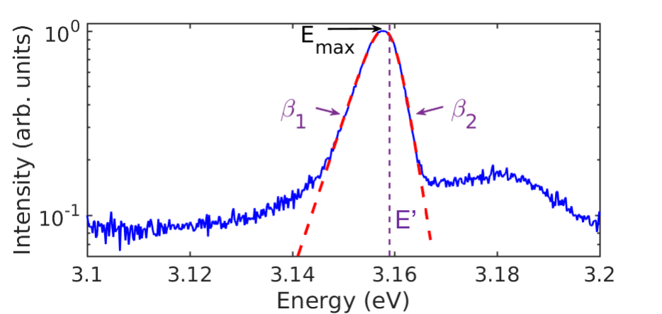
Figure A.4: A typoical IX photoluminescence spectrum (blue) and the result of the fitting procedure (red dashed).

We use the following generic function to describe the the IX spectrum:

$$I=f_{\theta}(E)=A\frac{\exp(\beta_{1}(E-E^{\prime}))}{1+\exp(\beta_{2}(E-E^{\prime}))}$$ (A5)

where $\theta=\{A,\beta_{1},E^{\prime},\beta_{2}\}$ is the set of parameters to be optimised. Our algorithm employs a least squares regression from a suitably predetermined initial condition. Note that the parameter $E^{\prime}$ does not correspond to the spectral maximum, $\mathrm{E}_{\mathrm{max}}$: the latter is thus obtained by a simple numerical search of the maximum value on a list of energy values applied to the model function $x\to f_{\theta_{0}}(x)$ where $\theta_{0}$ is the optimum in the sense of least squares.

Figure A.4 illustrates the relevance of the chosen fitting function and the quality of the line shape modelling.

A5 Estimation of density-dependent exciton energy shift.

We use two models to establish the relation between exciton density and the emission energy shift. The first model (Model NC, Sec. A5.1 ) is based on the solution of the coupled Schrödinger and Poisson equations Lefebvre et al. (2004). It accounts for the screening of the built-in electric field by the photocreated carriers, but neglects the correlations that can settle between them at low temperature and high densities. The second model (Model C, Sec. A5.2) accounts for both screening and correlations. Both models are described below.

A5.1 Self-consistent solution of SP equations (NC model)

Electron and hole wavefunctions are calculated by solving the 1D Schrödinger equation for the envelope function, $\Psi(z)$:

$$-\frac{\hbar^{2}}{2}\frac{\mathrm{d}}{\mathrm{d}z}\left(\frac{1}{m^{z}(z)}\frac{\mathrm{d}}{\mathrm{d}z}\Psi(z)\right)+V(z)\Psi(z)=E\Psi(z).$$ (A6)

Here $V(z)$ ($m^{z}(z)$) stands for the corresponding band potential (effective mass). We implement a second order finite difference scheme of uniform spatial step, $\Delta z$, that leads to the following secular equation

$$\left(H_{ij}+V_{i}\delta_{ij}\right)\Psi_{j}=E_{j}\Psi_{j}.$$ (A7)

Here $H\equiv(H_{ij})$ is a $N\times N$ tridiagonal matrix given by :

$$H=\left(\begin{array}[]{ccccc}D_{1}&U_{1}&&\dots&0\\ L_{2}&D_{2}&U_{2}&\dots&0\\ \vdots&\ddots&\ddots&\ddots&\vdots\\ &&&&U_{N-1}\\ 0&\dots&0&L_{N}&D_{N}\end{array}\right).$$ (A13)

Here $N$ is the number of nodes in the grid, while upper ($U_{i}$), lower ($L_{i}$) and diagonal ($D_{i}$) coefficients are given, for $1<i<N$, by

$$U_{i}= \frac{\hbar^{2}}{4\Delta z^{2}}\left(\frac{1}{m_{i+1}}+\frac{1}{m_{i}}\right)$$ (A14)

$$L_{i}= \frac{\hbar^{2}}{4\Delta z^{2}}\left(\frac{1}{m_{i}}+\frac{1}{m_{i-1}}\right)$$ (A15)

$$D_{i}= -\frac{\hbar^{2}}{4\Delta z^{2}}\left(\frac{1}{m_{i+1}}+\frac{2}{m_{i}}+\frac{1}{m_{i-1}}\right)$$ (A16)

Using $\Delta z\sim 0.1$ nm, the eigenvalues are computed with $\sim 10^{-6}$ relative precision. By applying the above formalism to both conduction and valence bands we obtain the corresponding ground state confinement energies. Their difference gives us the energy of the fundamental optical transition $E_{EH0}$.

Note, that we implement the simplest Born-Von Karman cyclic boundary conditions, that imply that the band potential is identical at the two boundaries of the active layer Gil (2014). One must bear in mind, however, that in reality the situation is more complex, and the potential drops across the active layer. Fermi level is known to be pinned at the surface, where a depletion region forms Segev and Van de Walle (2006); a two-dimensional electron gas resulting from residual doping and surface states accumulates on the back side of the active structure (at the bottom (Al,Ga)N/GaN interface). We checked that, for this sample structure, the Fermi level is well below the bottom of the QW Chiaruttini et al. (2019), which means that one should not expect the presence of the residual carriers in the active layer.

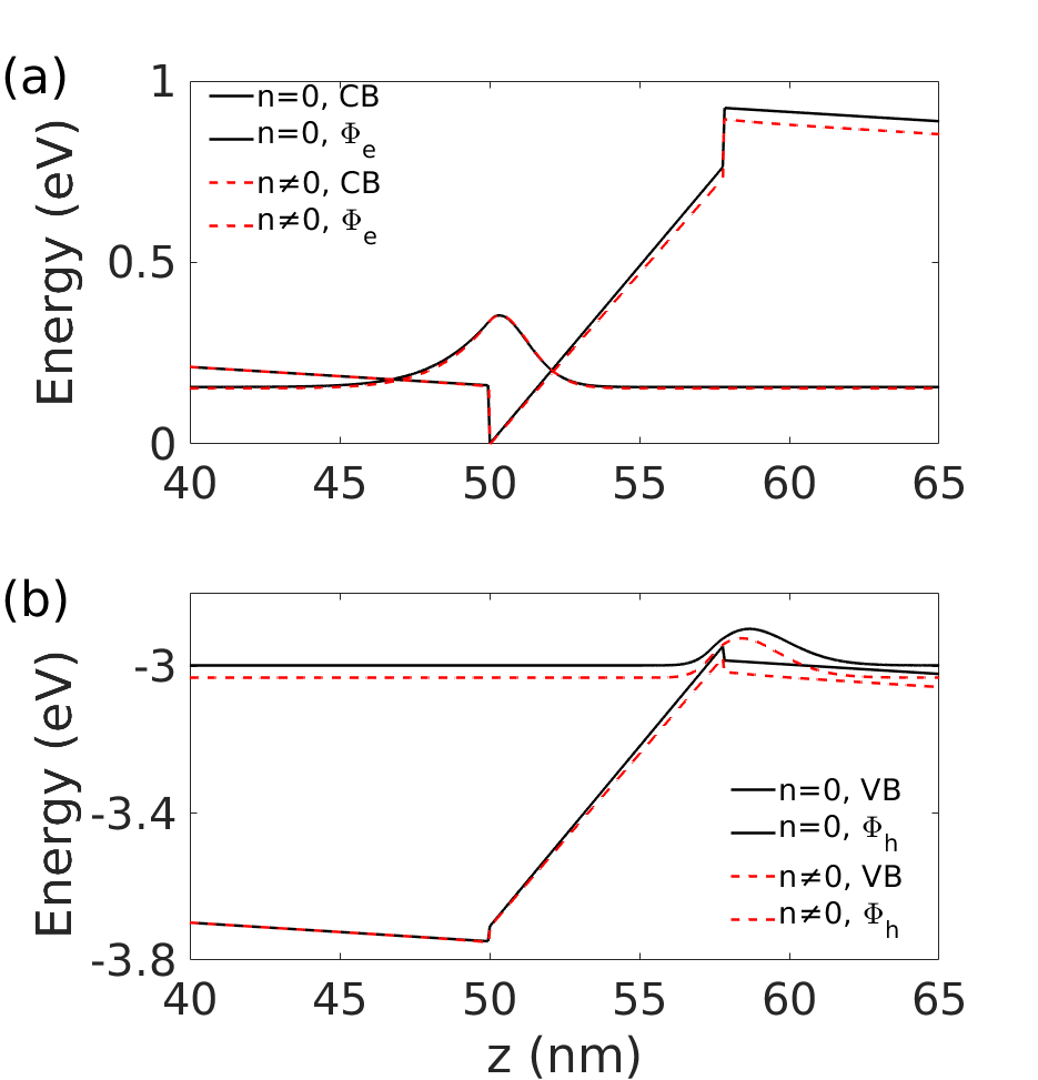
Figure A.5: Effect of the photoinjected carriers on the conduction (a) and valence (b) band diagram and wavefunction. The band profiles and wavefunctions are calculated for an empty QW (black lines) and for a pair density of $n=2\times 10^{11}$ cm^-2 (red dashed lines).

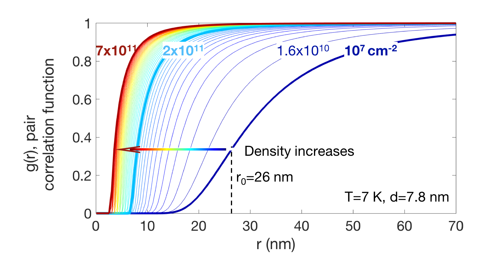
Figure A.6: Pair correlation function calculated for various values of the particle density at $T=7$ K and dipole length $d=7.8$ nm. Thick lines indicate the calculations in the low density limit ($n=10^{7}$ cm^-2, dark blue), at Mott density estimated in this work ($n=2\times 10^{11}$ cm^-2, cyan) and at $n=7\times 10^{11}$ cm^-2, corresponding to the saturation of $g(r)$. Dashed line poins $r_{0}$, the mean-field exclusion radius given by Eq. A22.

Photoinjected carriers affect the band potential that confines electrons and holes in the quantum well. For a given charge density profile $\rho(z)$ the resulting potential is given by the Poisson equation

$$\frac{\mathrm{d}}{\mathrm{d}z}\left(\varepsilon(z)\frac{\mathrm{d}}{\mathrm{d}z}V(z)\right)=-\rho(z)$$ (A17)

where $\varepsilon(z)$ is the local dielectric permittivity.

Using boundary conditions at $z=0$ (nullity of both electric potential and field) yields:

$$V(z)=-\int_{0}^{z}\mathrm{d}\xi\left[\frac{1}{\varepsilon(\xi)}\int_{0}^{\xi}\mathrm{d}\xi^{\prime}\,\rho(\xi^{\prime})\right].$$ (A18)

Thus, to account for the screening of the built-in potential by the photoinjected carriers we solve Poisson and Schrödinger equations self-consistently.

An example of such calculation for the electron-hole pair density $n=2\times 10^{11}$ cm^-2 and for $n=0$ in our sample is shown in Fig. A.5. One can see that the band diagram is less tilted in the presence of the carriers, due to the electrostatic screening effect. This implies the modification of both optical transition energy and the overlap $\Omega=\left|\int\mathrm{d}z\,\Phi_{e}(z)\Phi_{h}(z)\right|^{2}$ between the electron and hole wavefunctions ($\Omega$ is proportional to the radiative emission rate).

The transition energy increases almost linearly with density (figure not shown), at least in the density limit of interest. The slope $\phi_{0}=1.50\times 10^{-13}\textrm{ eV}\cdot\textrm{cm}^{2}$ is obtained from the linear fitting procedure. It differs only slightly from the value given by a simple ”plate capacitor” model

$$\phi_{0}^{PC}=\frac{e^{2}d}{\varepsilon}\approx 1.59\,10^{-13}\textrm{eV}\cdot\textrm{cm}^{2}$$ (A19)

This difference is due to the localization of the electron and hole wavefunctions in the inner part of the QW, which tends to reduce the effective QW width. The interaction energy $E_{int}$ given by $E_{int}=\phi_{0}n$ is shown in Fig. A.7 by the black line.

A5.2 Taking into account excitonic correlations (Model C)

A more accurate estimate of the excitonic density from the energy shift is based on taking into account the repulsive interactions between excitons. This means that one should go beyond the assumption of the uniform distribution of charges in the plane of the quantum well, on which the ”plate capacitor” and the Schrödinger-Poisson models are based.

The energy of an exciton in the field of its neighbors can be written as

$$E_{\mathrm{int}}^{\mathrm{corr}}(n,T)=\int n_{\ell}(r,T,n)U(r)d\mathbf{r}$$ (A20)

where $U(r)=\frac{2e^{2}}{4\pi\varepsilon}\left(\frac{1}{r}-\frac{1}{\sqrt{d^{2}+r^{2}}}\right)$ is the exciton-exciton interaction potential and $n_{\ell}(r,n,T)$ is the local density of excitons in equilibrium at temperature $T$ and for a global density $n$.

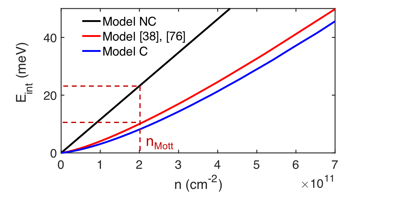
Figure A.7: (a) Interaction energy (or, equivalently, density-induced energy shift) as a function of particle density for $T=$ 7K. Model NC (self-consistent solution of the coupled Schrödinger and Poisson equations, Sec. A5.1), black line; Model C solved with (blue line) and without adaptive procedure, see Sec.A5.2. Dashed lines indicate the estimated Mott density and the corresponding interaction-induced energy shift.

According to Schindler and Zimmermann (2008); Ivanov et al. (2010), this local quantity is given by the equation

$$1-e^{-T_{0}(r)/T}=\left(1-e^{-T_{0}^{(0)}/T}\right)e^{-\left(U(r)+\phi_{0}(n_{\ell}-n)\right)/\left(k_{B}T\right)},$$ (A21)

where $k_{B}T_{0}(r)=\pi\hbar^{2}n_{\ell}(r,T,n)/2M$, represents the local chemical potential and $k_{B}T_{0}^{(0)}=\pi\hbar^{2}n/(2M)$, represents chemical potential in the $r\to\infty$ limit. The numerical resolution of this equation makes it possible to evaluate the local density $n_{\ell}(r,T,n)$ We push the numerical solution slightly further that the implementation presented in Ivanov et al. (2010). Our method is based on an adaptative calculation. The solution $n_{\ell}(r,T,n)$ of Eq. A21 is reinjected back in Eq. A20. The resulting $E_{\mathrm{int}}^{\mathrm{corr}}(n,T)$ is used to replace the ”mean field” term $\phi_{0}(n_{\ell}-n)$ in Eq. A21 by $E_{\mathrm{int}}^{\mathrm{corr}}(n_{\ell},T)-E_{\mathrm{int}}^{\mathrm{corr}}(n,T)$. The procedure is repeated until convergence.

The density dependence of the pair correlation fonction $g(r)=n_{\ell}(r,T,n)/n$ obtained within this model is shown in Fig. A.6. Because of the indirect nature of the excitons, a depletion area appears around each exciton. This area is characterized by an exclusion radius $r_{0}(T,n)$. One can clearly see in Fig. A.6, that the shape of the $g(r)$ gets steeper when the pair density increases. At low density the exclusion radius is given by the mean field value

$$r_{0}(n=0,T)=\left(\frac{e^{2}d^{2}}{4\pi\epsilon}\frac{1}{k_{B}T}\right)^{1/3},$$ (A22)

that is $\sim 30$ nm at $7$ K, and it shrinks down up to $\sim 5$ nm at highest densities. Interaction energy $E_{\mathrm{int}}(n,T)$ calculated within Model C is shown in Fig. A.7, for T=7 K. The red line corresponds to the implementation Refs. Schindler and Zimmermann (2008); Ivanov et al. (2010) and the blue line to the adaptive calculation described above and implemented in the main text to estimate the densities.

References

- Yudson and Lozovik (1976) V I Yudson and Yu E Lozovik, “A new mechanism for superconductivity: pairing between spatially separated electrons and holes,” Soviet Physics JETP 44, 389 (1976).
- Miller et al. (1985) D A B Miller, D S Chemla, T C Damen, A C Gossard, W Wiegmann, T H Wood, and C A Burrus, “Electric-Field Dependence of Optical-Absorption Near the Band-Gap of Quantum-Well Structures,” Phys. Rev. B 32, 1043–1060 (1985).
- Huber et al. (1998) T Huber, A Zrenner, W Wegscheider, and M Bichler, “Electrostatic Exciton Traps,” physica status solidi (a) 166, R5–R6 (1998).
- Ivanov et al. (1999) A L Ivanov, P B Littlewood, and H Haug, “Bose-Einstein statistics in thermalization and photoluminescence of quantum-well excitons,” Phys. Rev. B 59, 5032–5048 (1999).
- Butov et al. (1999) L V Butov, A A Shashkin, V T Dolgopolov, K L Campman, and A C Gossard, “Magneto-optics of the spatially separated electron and hole layers in GaAs/AlxGa1-xAs coupled quantum wells,” Phys. Rev. B 60, 8753–8758 (1999).
- High et al. (2008) Alex A High, Ekaterina E Novitskaya, Leonid V Butov, Micah Hanson, and Arthur C Gossard, “Control of exciton fluxes in an excitonic integrated circuit.” Science 321, 229–231 (2008).
- Butov (2017) L V Butov, “Excitonic devices,” Superlattices and Microstructures 108, 2–26 (2017).
- Lozovik and Berman (1996) Yu E Lozovik and O L Berman, “Phase transitions in a system of two coupled quantum wells,” Jetp Lett. 64, 573–579 (1996).
- High et al. (2012) A A High, J R Leonard, A T Hammack, M M Fogler, L V Butov, A V Kavokin, K L Campman, and A C Gossard, “Spontaneous coherence in a cold exciton gas,” Nature 483, 584–588 (2012).
- Shilo et al. (2013) Yehiel Shilo, Kobi Cohen, Boris Laikhtman, Ken West, Loren Pfeiffer, and Ronen Rapaport, “Particle correlations and evidence for dark state condensation in a cold dipolar exciton fluid,” Nature Communications 4, 1–7 (2013).
- Schinner et al. (2013) G J Schinner, J Repp, E Schubert, A K Rai, D Reuter, A D Wieck, A O Govorov, A W Holleitner, and J P Kotthaus, “Many-body correlations of electrostatically trapped dipolar excitons,” Phys. Rev. B 87, 205302 (2013).
- Cohen et al. (2016) Kobi Cohen, Yehiel Shilo, Ken West, Loren Pfeiffer, and Ronen Rapaport, “Dark High Density Dipolar Liquid of Excitons,” Nano Lett. 16, 3726–3731 (2016).
- Butov (2016) L V Butov, “Collective phenomena in cold indirect excitons,” J. Exp. Theor. Phys. 149, 505 (2016).
- Combescot et al. (2017) Monique Combescot, Roland Combescot, and François Dubin, “Bose–Einstein condensation and indirect excitons: a review,” Rep. Prog. Phys. 80, 066501 (2017).
- Anankine et al. (2017) Romain Anankine, Mussie Beian, Suzanne Dang, Mathieu Alloing, Edmond Cambril, Kamel Merghem, Carmen Gomez Carbonell, Aristide Lemaître, and François Dubin, “Quantized Vortices and Four-Component Superfluidity of Semiconductor Excitons,” Phys. Rev. Lett. 118, 127402 (2017).
- Misra et al. (2018) Subhradeep Misra, Michael Stern, Arjun Joshua, Vladimir Umansky, and Israel Bar-Joseph, “Experimental Study of the Exciton Gas-Liquid Transition in Coupled Quantum Wells,” Phys. Rev. Lett. 120, 047402 (2018).
- Laikhtman and Rapaport (2009a) B Laikhtman and Ronen Rapaport, “Exciton correlations in coupled quantum wells and their luminescence blue shift,” Phys. Rev. B 80, 195313–12 (2009a).
- Zimmermann et al. (1978) R Zimmermann, K Kilimann, W D Kraeft, D Kremp, and G Röpke, “Dynamical screening and self-energy of excitons in the electron–hole plasma,” phys. stat. sol. (b) 90, 175–187 (1978).
- Mott (1968) N F Mott, “Metal-Insulator Transition,” Rev. Mod. Phys. 40, 677–683 (1968).
- Ben-Tabou de Leon and Laikhtman (2003) S Ben-Tabou de Leon and B Laikhtman, “Mott transition, biexciton crossover, and spin ordering in the exciton gas in quantum wells,” Phys. Rev. B 67, 235315 (2003).
- Nikolaev and Portnoi (2004) V V Nikolaev and M E Portnoi, “Theory of excitonic Mott transition in double quantum wells,” phys. stat. sol. (c) 1, 1357–1362 (2004).
- Stern et al. (2008) M Stern, V Garmider, V Umansky, and I Bar-Joseph, “Mott Transition of Excitons in Coupled Quantum Wells,” Phys. Rev. Lett. 100, 256402 (2008).
- Snoke (2008) David Snoke, “Predicting the ionization threshold for carriers in excited semiconductors,” Solid State Communications 146, 73 (2008).
- Byrnes et al. (2010) Tim Byrnes, Patrik Recher, and Yoshihisa Yamamoto, “Mott transitions of exciton polaritons and indirect excitons in a periodic potential,” Phys. Rev. B 81, 205312–13 (2010).
- Kiršanskė et al. (2016) Gabija Kiršanskė, Petru Tighineanu, Raphaël S Daveau, Javier Miguel-Sánchez, Peter Lodahl, and Søren Stobbe, “Observation of the exciton Mott transition in the photoluminescence of coupled quantum wells,” Phys. Rev. B 94, 155438 (2016).
- Vignesh and Nithiananthi (2020) G Vignesh and P Nithiananthi, “Hartree-Fock approximation for exciton Mott transition in double quantum well: Direct and indirect exciton diamagnetism,” Physica E: Low-dimensional Systems and Nanostructures , 114008 (2020).
- Kappei et al. (2005) L Kappei, J Szczytko, F Morier-Genoud, and B Deveaud, “Direct Observation of the Mott Transition in an Optically Excited Semiconductor Quantum Well,” Phys. Rev. Lett. 94, 147403 (2005).
- Deveaud et al. (2005) B Deveaud, L Kappei, J Berney, F Morier-Genoud, M T Portella-Oberli, J Szczytko, and C Piermarocchi, “Excitonic effects in the luminescence of quantum wells,” Chemical Physics 318, 104–117 (2005).
- Nikolaev and Portnoi (2008) V V Nikolaev and M E Portnoi, “Theory of the excitonic Mott transition in quasi-two-dimensional systems,” Superlattices and Microstructures 43, 460–464 (2008).
- Sekiguchi and Shimano (2017) Fumiya Sekiguchi and Ryo Shimano, “Rate Equation Analysis of the Dynamics of First-order Exciton Mott Transition,” Journal of the Physical Society of Japan 86, 103702 (2017).
- Mock et al. (1978) J B Mock, G A Thomas, and M Combescot, “Entropy ionization of an exciton gas,” Solid State Communications 25, 279–282 (1978).
- Chiaruttini et al. (2019) François Chiaruttini, Thierry Guillet, Christelle Brimont, Benoit Jouault, Pierre Lefebvre, Jessica Vives, Sebastien Chenot, Yvon Cordier, Benjamin Damilano, and Maria Vladimirova, “Trapping Dipolar Exciton Fluids in GaN/(AlGa)N Nanostructures,” Nano Lett. 19, 4911 (2019).
- Gil (2014) Bernard Gil, III-Nitride Semiconductors and their Modern Devices (Springer, 2014).
- Bernardini and Fiorentini (1998) Fabio Bernardini and Vincenzo Fiorentini, “Macroscopic polarization and band offsets at nitride heterojunctions,” Phys. Rev. B 57, R9427–R9430 (1998).
- Leroux et al. (1998) M Leroux, N Grandjean, M Laügt, J Massies, B Gil, P Lefebvre, and P Bigenwald, “Quantum confined Stark effect due to built-in internal polarization fields in (Al,Ga)N/GaN quantum wells,” Phys. Rev. B 58, R13371–R13374 (1998).
- Grandjean et al. (1999) N Grandjean, B Damilano, S Dalmasso, M Leroux, M Laügt, and J Massies, “Built-in electric-field effects in wurtzite AlGaN/GaN quantum wells,” J. Appl. Phys. 86, 3714 (1999).
- Kash et al. (1991) J A Kash, M Zachau, E E Mendez, J M Hong, and T Fukuzawa, “Fermi-Dirac distribution of excitons in coupled quantum wells,” Phys. Rev. Lett. 66, 2247–2250 (1991).
- Schindler and Zimmermann (2008) Christoph Schindler and Roland Zimmermann, “Analysis of the exciton-exciton interaction in semiconductor quantum wells,” Phys. Rev. B 78, 045313 (2008).
- Laikhtman and Rapaport (2009b) B. Laikhtman and R. Rapaport, “Correlations in a two-dimensional Bose gas with long-range interaction,” Europhysics Letters 87, 27010 (2009b).
- Mazuz-Harpaz et al. (2017) Yotam Mazuz-Harpaz, Kobi Cohen, and Ronen Rapaport, “Condensation to a strongly correlated dark fluid of two dimensional dipolar excitons,” Superlattices and Microstructures 108, 88–97 (2017).
- Zimmermann (1987) Roland Zimmermann, Many-Particle Theory of Highly Excited Semiconductors (BSB Teubner, 1987).
- Note (1) Note, that so-called magnetoexcitons characterised by linear energy shift under magnetic field are routinely observed in GaAs when magnetic length becomes smaller than exciton Bohr radius. This regime is never achieved in this work.
- Kuznetsova et al. (2017) Y Y Kuznetsova, C J Dorow, E V Calman, L V Butov, J Wilkes, E A Muljarov, K L Campman, and A C Gossard, “Transport of indirect excitons in high magnetic fields,” Phys. Rev. B 95, 125304 (2017).
- Dorow et al. (2017) C J Dorow, M W Hasling, E V Calman, L V Butov, J Wilkes, K L Campman, and A C Gossard, “Spatially resolved and time-resolved imaging of transport of indirect excitons in high magnetic fields,” Phys. Rev. B 95, 235308 (2017).
- Grandjean et al. (2000) N Grandjean, B Damilano, J Massies, G Neu, M Teissere, I Grzegory, S Porowski, M Gallart, P Lefebvre, B Gil, and M Albrecht, “Optical properties of GaN epilayers and GaN/AlGaN quantum wells grown by molecular beam epitaxy on GaN(0001) single crystal substrate,” J. Appl. Phys. 88, 183–187 (2000).
- Lefebvre et al. (1999) Pierre Lefebvre, Jacques Allègre, Bernard Gil, Henry Mathieu, Nicolas Grandjean, Mathieu Leroux, Jean Massies, and Pierre Bigenwald, “Time-resolved photoluminescence as a probe of internal electric fields in GaN-(GaAl)N quantum wells,” Phys. Rev. B 59, 15363–15367 (1999).
- Fedichkin et al. (2015) F. Fedichkin, P. Andreakou, B. Jouault, M. Vladimirova, T. Guillet, C. Brimont, P. Valvin, T. Bretagnon, A. Dussaigne, N. Grandjean, and P. Lefebvre, “Transport of dipolar excitons in (Al,Ga)N/GaN quantum wells,” Phys. Rev. B 91, 205424 (2015).
- Rosales et al. (2013) D Rosales, T Bretagnon, B Gil, A Kahouli, J Brault, B Damilano, J Massies, M V Durnev, and A V Kavokin, “Excitons in nitride heterostructures: From zero- to one-dimensional behavior,” Phys. Rev. B 88, 125437 (2013).
- Rossbach et al. (2014) G Rossbach, J Levrat, G Jacopin, M Shahmohammadi, J F Carlin, J D Ganière, R Butté, B Deveaud, and N Grandjean, “High-temperature Mott transition in wide-band-gap semiconductor quantum wells,” Phys. Rev. B 90, 201308 (2014).
- Fedichkin et al. (2016) F Fedichkin, T Guillet, P Valvin, B Jouault, C Brimont, T Bretagnon, L Lahourcade, N Grandjean, P Lefebvre, and M Vladimirova, “Room-Temperature Transport of Indirect Excitons in (Al,Ga)N/GaN Quantum Wells,” Phys. Rev. Applied 6, 014011 (2016).
- Lefebvre et al. (2004) P Lefebvre, S Kalliakos, T Bretagnon, P Valvin, T Taliercio, B Gil, N Grandjean, and J Massies, “Observation and modeling of the time-dependent descreening of internal electric field in a wurtzite GaN/Al0.15Ga0.85N quantum well after high photoexcitation,” Phys. Rev. B 69, 035307 (2004).
- Remeika et al. (2009) M Remeika, J C Graves, A T Hammack, A D Meyertholen, M M Fogler, L V Butov, M Hanson, and A C Gossard, “Localization-Delocalization Transition of Indirect Excitons in Lateral Electrostatic Lattices,” Phys. Rev. Lett. 102, 186803–4 (2009).
- Leonard et al. (2012) J R Leonard, M Remeika, M K Chu, Y Y Kuznetsova, A A High, L V Butov, J Wilkes, M Hanson, and A C Gossard, “Transport of indirect excitons in a potential energy gradient,” Appl. Phys. Lett. 100, 231106–231105 (2012).
- Rapaport et al. (2006) Ronen Rapaport, Gang Chen, and Steven H. Simon, “Nonlinear dynamics of a dense two-dimensional dipolar exciton gas,” Phys. Rev. B 73, 033319 (2006).
- Ivanov (2002) A L Ivanov, “Quantum diffusion of dipole-oriented indirect excitons in coupled quantum wells,” EPL 59, 586–591 (2002).
- Lozovik and Ruvinskii (1997) Yu E Lozovik and A M Ruvinskii, “Magnetoexciton absorption in coupled quantum wells,” J. Exp. Theor. Phys. 85, 979–988 (1997).
- Butov et al. (2001) L V Butov, C W Lai, D S Chemla, Yu E Lozovik, K L Campman, and A C Gossard, “Observation of Magnetically Induced Effective-Mass Enhancement of Quasi-2D Excitons,” Phys. Rev. Lett. 87, 216804 (2001).
- Lozovik et al. (2002) Yu E Lozovik, I V Ovchinnikov, S Yu Volkov, L V Butov, and D S Chemla, “Quasi-two-dimensional excitons in finite magnetic fields,” Phys. Rev. B 65, 235304 (2002).
- Edelstein et al. (1989) Warren Edelstein, Harold N Spector, and Richard Marasas, “Two-dimensional excitons in magnetic fields,” Phys. Rev. B 39, 7697–7704 (1989).
- Stépnicki et al. (2015) Piotr Stépnicki, Barbara Piétka, François Morier-Genoud, Benoit Deveaud, and Michał Matuszewski, “Analytical method for determining quantum well exciton properties in a magnetic field,” Phys. Rev. B 91, 195302 (2015).
- Arnardottir et al. (2012) K B Arnardottir, O Kyriienko, and I A Shelykh, “Hall effect for indirect excitons in an inhomogeneous magnetic field,” Phys. Rev. B 86, 245311 (2012).
- Wilkes and Muljarov (2017) J Wilkes and E A Muljarov, “Excitons and polaritons in planar heterostructures in external electric and magnetic fields: A multi-sub-level approach,” Superlattices and Microstructures (2017).
- Wilkes and Muljarov (2016) J Wilkes and E A Muljarov, “Exciton effective mass enhancement in coupled quantum wells in electric and magnetic fields,” New J. Phys. 18, 023032 (2016).
- Arseev and Dzyubenko (1998) P I Arseev and A B Dzyubenko, “Exciton magnetotransport in two-dimensional systems: Weak-localization effects,” J. Exp. Theor. Phys. 87, 200–209 (1998).
- Bugajski et al. (1986) M Bugajski, W Kuszko, and K Regiński, “Diamagnetic shift of exciton energy levels in GaAs-GaAlAs quantum wells,” Solid State Communications 60, 669 (1986).
- Bigenwald et al. (1999) P Bigenwald, P Lefebvre, T Bretagnon, and B Gil, “Confined Excitons in GaN–AlGaN Quantum Wells,” Phys. Status solidi (b) 216, 371–374 (1999).
- (67) Pierre Bigenwald, Alexey Kavokin, Bernard Gil, and Pierre Lefebvre, “Exclusion principle and screening of excitons in GaN/AlxGa1−xn quantum wells,” .
- Hangleiter et al. (2015) Andreas Hangleiter, Zuanming Jin, Marina Gerhard, Dimitry Kalincev, Torsten Langer, Heiko Bremers, Uwe Rossow, Martin Koch, Mischa Bonn, and Dmitry Turchinovich, “Efficient formation of excitons in a dense electron-hole plasma at room temperature,” Phys. Rev. B 92, 241305 (2015).
- Bigenwald et al. (2000) Pierre Bigenwald, Alexey Kavokin, Bernard Gil, and Pierre Lefebvre, “Electron-hole plasma effect on excitons in GaN/AlxGa1−x quantum wells,” Phys. Rev. B 61, 15621–15624 (2000).
- Liu et al. (2016) W Liu, R Butté, A Dussaigne, N Grandjean, B Deveaud, and G Jacopin, “Carrier-density-dependent recombination dynamics of excitons and electron-hole plasma in m-plane InGaN/GaN quantum wells,” Phys. Rev. B 94, 195411 (2016).
- Vurgaftman et al. (2001) I Vurgaftman, J R Meyer, and L R Ram-Mohan, “Band parameters for III–V compound semiconductors and their alloys,” J. Appl. Phys. 89, 5815–5875 (2001).
- Vurgaftman and Meyer (2003) I Vurgaftman and J R Meyer, “Band parameters for nitrogen-containing semiconductors,” J. Appl. Phys. 94, 3675–3696 (2003).
- Kabi et al. (2009) S Kabi, D Biswas, and S Panda, “Calculations for the band lineup and band offsets of algan/gan qws and effects of electric field on the photoluminescence,” in 4th International Conference on Computers and Devices for Communication (CODEC) (2009).
- Rickert et al. (2002) K A Rickert, A B Ellis, Jong Kyu Kim, Jong-Lam Lee, F J Himpsel, F Dwikusuma, and T F Kuech, “X-ray photoemission determination of the Schottky barrier height of metal contacts to n–GaN and p–GaN,” J. Appl. Phys. 92, 6671–6678 (2002).
- Segev and Van de Walle (2006) D Segev and C G Van de Walle, “Origins of Fermi-level pinning on GaN and InN polar and nonpolar surfaces,” EPL 76, 305–311 (2006).
- Ivanov et al. (2010) A. L. Ivanov, E. A. Muljarov, L. Mouchliadis, and R. Zimmermann, “Comment on ”photoluminescence ring formation in coupled quantum wells: Excitonic versus ambipolar diffusion”,” Phys. Rev. Lett. 104, 179701 (2010).