Which form of the molecular Hamiltonian is the most suitable for simulating the nonadiabatic quantum dynamics at a conical intersection?

Abstract

Choosing an appropriate representation of the molecular Hamiltonian is one of the challenges faced by simulations of the nonadiabatic quantum dynamics around a conical intersection. The adiabatic, exact quasidiabatic, and strictly diabatic representations are exact and unitary transforms of each other, whereas the approximate quasidiabatic Hamiltonian ignores the residual nonadiabatic couplings in the exact quasidiabatic Hamiltonian. A rigorous numerical comparison of the four different representations is difficult because of the exceptional nature of systems where the four representations can be defined exactly and the necessity of an exceedingly accurate numerical algorithm that avoids mixing numerical errors with errors due to the different forms of the Hamiltonian. Using the quadratic Jahn-Teller model and high-order geometric integrators, we are able to perform this comparison and find that only the rarely employed exact quasidiabatic Hamiltonian yields nearly identical results to the benchmark results of the strictly diabatic Hamiltonian, which is not available in general. In this Jahn-Teller model and with the same Fourier grid, the commonly employed approximate quasidiabatic Hamiltonian led to inaccurate wavepacket dynamics, while the Hamiltonian in the adiabatic basis was the least accurate, due to the singular nonadiabatic couplings at the conical intersection.

I Introduction

Many physical and chemical phenomena proceed via conical intersections—nuclear geometries where adiabatic potential energy surfaces of two or more electronic states intersect.[1, 2, 3, 4, 5] The conical intersections, which are much more ubiquitous[6, 7, 8, 9] than previously believed, are responsible for the failure of the celebrated Born–Oppenheimer approximation that treats the electronic and nuclear motions in molecules separately. To correctly describe processes involving conical intersections, methods going beyond[10, 11, 12, 13, 14, 15, 16, 17, 18] the Born–Oppenheimer approximation must be used. Often, it is necessary to take into account multiple strongly coupled electronic states[19, 10, 20] and, in the adiabatic basis, one must consider the geometric phase effect—the sign change of adiabatic electronic states along a closed path encircling a conical intersection.[21, 22, 23, 24, 25, 26, 27, 28, 29, 30, 31, 32]

Simulating the nonadiabatic quantum dynamics at a conical intersection using the adiabatic Hamiltonian, obtained from the electronic structure calculations, is problematic due to both the geometric phase effect[21, 24, 27, 28, 29, 30, 31, 32] and singular nonadiabatic couplings.[20] These are rectified by a unitary transformation into the equivalent exact quasidiabatic Hamiltonian. Unlike the adiabatic electronic states, which are only coupled through the nonadiabatic couplings, the quasidiabatic states have both the residual, presumably small, nonadiabatic couplings and the diabatic couplings—the off-diagonal elements of the potential energy matrix. However, the exact quasidiabatic Hamiltonian is rarely used. Instead, the approximate quasidiabatic Hamiltonian, which ignores the residual nonadiabatic couplings, is almost always used due to its simplicity. The separable form of the approximate quasidiabatic Hamiltonian allows using a wider range of time propagation schemes,[33, 34, 35, 36] including the well-known split-operator algorithm,[37, 38, 39] but ignoring the residual nonadiabatic couplings decreases the accuracy.[40] The strictly diabatic Hamiltonian, with only diabatic couplings and no nonadiabatic couplings, would be the most suitable for the nonadiabatic quantum dynamics simulation. However, in typical systems, the strictly diabatic states only exist in general when an infinite number of electronic states are considered.[41, 42]

Advantages and disadvantages of various Hamiltonians have been explored by numerous comparisons of the nonadiabatic quantum dynamics simulated with different Hamiltonians: To name a few, there exist comparisons between the strictly diabatic and approximate quasidiabatic Hamiltonians,[43, 42, 44, 45, 46] between the adiabatic and approximate quasidiabatic Hamiltonians,[47, 48, 49] between the adiabatic and exact quasidiabatic Hamiltonians,[50, 51] and between the adiabatic and strictly diabatic Hamiltonians.[52, 53, 31] To the best of our knowledge, no study has compared all four different Hamiltonians—the adiabatic, exact quasidiabatic, approximate quasidiabatic, and strictly diabatic Hamiltonians—on a single system. A rigorous comparison is challenging because one must have both an appropriate system, where the different Hamiltonians are defined exactly, and a highly-accurate numerical integrator, which allows separating numerical errors from the errors due to using different forms of the Hamiltonian.

The two-dimensional, two-state quadratic $E\otimes e$ Jahn–Teller model[54, 55, 46] is perfect for this comparison because analytical expressions exist for potential energy surfaces and nonadiabatic couplings in both the adiabatic and quasidiabatic representations and because this model has—exceptionally—a strictly diabatic Hamiltonian.

As for numerical integrators, the split-operator algorithms[37, 38, 39] are applicable to both the approximate quasidiabatic and strictly diabatic Hamiltonians because these Hamiltonians are separable, i.e., they can be expressed as sums of terms depending purely on either the position or momentum operator. In contrast, neither the adiabatic nor exact quasidiabatic Hamiltonian is separable due to the nonvanishing nonadiabatic couplings. Although the split-operator algorithms cannot be used, the wavepacket can be propagated with the implicit midpoint method.[36, 56] Both the split-operator and implicit midpoint methods preserve most geometric properties of the exact solution (such as norm conservation, stability, and time reversibility) and, in addition, can be symmetrically composed[57, 58, 59, 36] to obtain integrators of arbitrary even order in the time step.[60, 61] By taking advantage of the suitable model and high-order geometric integrators, we numerically compared the wavepacket and observables obtained from simulations with the different Hamiltonians: the adiabatic, exact quasidiabatic, approximate quasidiabatic, and strictly diabatic Hamiltonians.

II Theory

The molecular Hamiltonian can be partitioned as $\mathcal{H}=\mathcal{T}_{\mathrm{N}}+\mathcal{H}_{\mathrm{e}}(Q)$, where $\mathcal{T}_{\mathrm{N}}$ is the nuclear kinetic energy operator and $\mathcal{H}_{\mathrm{e}}(Q)$ denotes the electronic Hamiltonian, which depends parametrically on the $D$-dimensional vector $Q$ of nuclear coordinates. Using the adiabatic electronic states $|n(Q)\rangle$, obtained by solving the time-independent Schrödinger equation

$$\mathcal{H}_{\mathrm{e}}(Q)|n(Q)\rangle=V_{n}(Q)|n(Q)\rangle,$$ (1)

one can establish an approximate ansatz

$$|\Psi(Q,t)\rangle =\sum_{n=1}^{S}\psi_{n}(Q,t)|n(Q)\rangle$$

$$=\sum_{n=1}^{S}[\psi_{n}(Q,t)e^{-iA_{n}(Q)}][e^{iA_{n}(Q)}|n(Q)\rangle]$$ (2)

for the solution of the time-dependent Schrödinger equation

$$i\hbar\frac{\partial}{\partial t}|\Psi(Q,t)\rangle=\mathcal{H}|\Psi(Q,t)\rangle;$$ (3)

here, $\psi_{n}(Q,t)$, $V_{n}(Q)$, and $e^{iA_{n}(Q)}$ are the time-dependent nuclear wavefunction, potential energy surface, and coordinate-dependent phase factor associated with the $n$th adiabatic electronic state. The Born–Huang expansion[62] in Eq. (2) is not exact unless the sum includes an infinite number of terms but can be very accurate if a finite number $S$ of electronic states are chosen wisely.[63, 64, 10]

One is free to choose an overall phase $A_{n}(Q)$ in Eq. (2) because if $|n(Q)\rangle$ is a normalized solution of Eq. (1), then so is $e^{iA_{n}(Q)}|n(Q)\rangle$. Unless $A_{n}(Q)$ is carefully chosen, however, the adiabatic states and, therefore, also the wavepackets undergo a sign change along a closed path encircling a conical intersection.[21, 3, 22, 23, 24, 25, 26, 32, 27, 28, 29, 30, 31, 29] In Sec. S4 of the supplementary material, we show that neglecting this double-valuedness of the wavepackets is detrimental to accuracy. Instead, in what follows, we set phases $A_{n}{(Q)}$ appropriately (see Sec. S1 of the supplementary material) to ensure the single-valuedness of both the adiabatic states and the wavepackets. In other words, we include the “geometric phase” in the adiabatic states in order to obtain the best possible results in the adiabatic representation. From now on, we absorb the overall phase factors $e^{-iA_{n}(Q)}$ and $e^{iA_{n}(Q)}$ into the nuclear wavefunctions $\psi_{n}(Q,t)$ and adiabatic states $|n(Q)\rangle$.

The time-dependent Schrödinger equation in the adiabatic representation,

$$i\hbar\frac{d}{dt}\bm{\psi}(t)=\hat{\mathbf{H}}_{\mathrm{ad}}\bm{\psi}(t),$$ (4)

is obtained by substituting ansatz (2) into Eq. (3) and projecting onto electronic states $\langle m(Q)|$ for $m\in\{1,\dots,S\}$. Note that we have introduced the representation-independent matrix notation: bold font indicates either an $S\times S$ matrix, i.e., an electronic operator, or $S$-dimensional vector, and the hat $\hat{}$ indicates a nuclear operator. In particular, $(\hat{\mathbf{H}}_{\mathrm{ad}})_{mn}=\langle m|\mathcal{H}|n\rangle$ is the adiabatic Hamiltonian, and $\bm{\psi}(t)$ denotes the molecular wavepacket in the adiabatic representation with components $\psi_{n}(t)$; henceforth, $m,n\in\{1,\dots,S\}$ unless otherwise stated. The formal solution of Eq. (4) for a given initial condition $\bm{\psi}(0)$ is

$$\bm{\psi}_{\mathrm{ad}}(t):=\hat{\mathbf{U}}_{\mathrm{ad}}(t)\bm{\psi}(0),$$ (5)

where $\hat{\mathbf{U}}_{\mathrm{ad}}(t)$ denotes the exact evolution operator $\hat{\mathbf{U}}_{i}(t):=\exp(-i\hat{\mathbf{H}}_{i}t/\hbar)$ with $i=\mathrm{ad}$. The adiabatic Hamiltonian $\hat{\mathbf{H}}_{\mathrm{ad}}$ is often expressed as

$$\hat{\mathbf{H}}_{\mathrm{ad}}=\frac{1}{2M}[\hat{P}^{2}\mathbf{1}-2i\hbar\mathbf{F}_{\mathrm{ad}}(\hat{Q})\cdot\hat{P}-\hbar^{2}\mathbf{G}_{\mathrm{ad}}(\hat{Q})]+\mathbf{V}_{\mathrm{ad}}(\hat{Q}),$$ (6)

where we have used the matrix notation for the diagonal adiabatic potential energy matrix $[\mathbf{V}_{\mathrm{ad}}(Q)]_{mn}:=V_{n}(Q)\delta_{mn}$, nonadiabatic vector couplings $[\mathbf{F}_{\mathrm{ad}}(Q)]_{mn}:=\langle m(Q)|\nabla n(Q)\rangle$, and nonadiabatic scalar couplings $[\mathbf{G}_{\mathrm{ad}}(Q)]_{mn}:=\langle m(Q)|\nabla^{2}n(Q)\rangle$. The $D$-dimensional vector $P$ is the nuclear momentum conjugate to $Q$ and the dot $\cdot$ denotes a dot product in the $D$-dimensional nuclear vector space; we use the mass-scaled coordinates for simplicity.

Expressing the nonadiabatic vector couplings as

$$[\mathbf{F}_{\mathrm{ad}}(Q)]_{mn}=\frac{\langle m(Q)|\nabla\mathcal{H}_{\mathrm{e}}(Q)|n(Q)\rangle}{V_{n}(Q)-V_{m}(Q)},\quad m\neq n,$$ (7)

shows that they are singular at a conical intersection,[65] which is a nuclear geometry $Q_{0}$ where $V_{m}(Q_{0})=V_{n}(Q_{0})$ for $m\neq n$.[11, 20, 66] This singularity causes problems for the nonadiabatic dynamics simulations, and especially for the grid-based methods because an infinitely dense grid would be required to describe the singularity. The singularity, however, can be removed by a coordinate-dependent unitary transformation of Hamiltonian (6) into its quasidiabatic representation,

$$\hat{\mathbf{H}}_{\text{qd-exact}}=\mathbf{S}(\hat{Q})\hat{\mathbf{H}}_{\mathrm{ad}}\mathbf{S}(\hat{Q})^{\dagger}$$

$$=\frac{1}{2M}[\hat{P}^{2}\mathbf{1}-2i\hbar\mathbf{F}_{\mathrm{qd}}(\hat{Q})\cdot\hat{P}-\hbar^{2}\mathbf{G}_{\mathrm{qd}}(\hat{Q})]+\mathbf{V}_{\mathrm{qd}}(\hat{Q}),$$ (8)

where $\mathbf{F}_{\mathrm{qd}}(Q)$ and $\mathbf{G}_{\mathrm{qd}}(Q)$ denote the residual nonadiabatic vector and scalar couplings, respectively. Different transformation matrices $\mathbf{S}(Q)$ are obtained by different quasidiabatization schemes,[65] which include the block-diagonalization of the reference Hamiltonian matrix,[44, 67, 68, 69] integration of the nonadiabatic couplings,[70, 71, 72, 73, 74] use of the molecular properties,[75, 76, 77, 78, 79, 80, 81] and construction of regularized quasidiabatic states.[46, 43, 82] We have chosen the regularized diabatization scheme because it is simple to implement and because it removes the conical intersection singularity reliably and efficiently.[83] The choice of quasidiabatization affects the magnitude of the residual couplings and, therefore, their importance for the accuracy of nonadiabatic simulations.[40]

The initial state can be propagated with $\hat{\mathbf{H}}_{\text{qd-exact}}$ instead of $\hat{\mathbf{H}}_{\mathrm{ad}}$ to obtain the solution

$$\bm{\psi}_{\text{qd-exact}}(t):=\mathbf{S}(\hat{Q})^{\dagger}\hat{\mathbf{U}}_{\text{qd-exact}}(t)\mathbf{S}(\hat{Q})\bm{\psi}(0),$$ (9)

which is equivalent to $\bm{\psi}_{\mathrm{ad}}(t)$. However, it is much more common to use the simpler approximate quasidiabatic Hamiltonian

$$\hat{\mathbf{H}}_{\text{qd-approx}}=\frac{\hat{P}^{2}}{2M}\mathbf{1}+\mathbf{V}_{\mathrm{qd}}(\hat{Q}).$$ (10)

This approximation is typically justified only heuristically by referring to the “small” magnitude of the residual nonadiabatic couplings. Nevertheless, the solution

$$\bm{\psi}_{\text{qd-approx}}(t) :=\mathbf{S}(\hat{Q})^{\dagger}\hat{\mathbf{U}}_{\text{qd-approx}}(t)\mathbf{S}(\hat{Q})\bm{\psi}(0)$$

$$\approx\bm{\psi}_{\text{qd-exact}}(t),$$ (11)

obtained using $\hat{\mathbf{H}}_{\text{qd-approx}}$ is not exact and would still be only approximate even if evaluated numerically exactly.

We have numerically compared the three different solutions, $\bm{\psi}_{\mathrm{ad}}(t)$, $\bm{\psi}_{\text{qd-exact}}(t)$, and $\bm{\psi}_{\text{qd-approx}}(t)$ using the archetypal quadratic $E\otimes e$ Jahn–Teller model.[54, 46] In the model, two electronic states labeled by $n=1$ and $n=2$ are coupled by doubly degenerate normal modes $Q_{1}$ and $Q_{2}$. We express the potential energy surface in polar coordinates—the radius $\rho(Q):=\sqrt{Q_{1}^{2}+Q_{2}^{2}}$ and polar angle $\phi(Q):=\arctan{(Q_{2}/Q_{1})}$ in the space of the degenerate normal modes.[54, 46] Also, we work in natural units (n.u.) by setting $k=M=\hbar=1$ n.u., where $M$ is the mass associated with the degenerate normal modes, and $\hbar\omega=\hbar\sqrt{k/M}=1$ n.u. is a quantum of the vibrational energy of these modes.[54, 55]

The adiabatic potential energy surfaces are $V_{1}(Q)=V_{+}(Q)$ and $V_{2}(Q)=V_{-}(Q)$, where $V_{\pm}(Q):=E_{0}(Q)\pm E_{\mathrm{cpl}}(Q)$ depends on the harmonic potential energy $E_{0}(Q):=k\rho(Q)^{2}/2$ and Jahn–Teller coupling[54, 46]

$$E_{\mathrm{cpl}}(Q):=\rho(Q)[c_{1}^{2}+2c_{1}c_{2}\rho(Q)\cos{3\phi(Q)}+c_{2}^{2}\rho(Q)^{2}]^{1/2}.$$ (12)

The nonadiabatic vector coupling is[54, 46]

$$\mathbf{F}_{\mathrm{ad}}(Q)=-i\begin{pmatrix}\nabla\alpha(Q)&e^{2i\alpha(Q)}\nabla\theta(Q)\\ e^{-2i\alpha(Q)}\nabla\theta(Q)&-\nabla\alpha(Q)\end{pmatrix}$$ (13)

with $\alpha(Q):=\phi(Q)/2$ and

$$\theta(Q):=\frac{1}{2}\arctan{\frac{c_{1}\rho(Q)\sin{\phi(Q)}-c_{2}\rho(Q)^{2}\sin{2\phi(Q)}}{c_{1}\rho(Q)\cos{\phi(Q)}+c_{2}\rho(Q)^{2}\cos{2\phi(Q)}}};$$ (14)

in our study, the coupling coefficients were $c_{1}=1$ n.u. and $c_{2}=0.25$ n.u. Unlike the potential energy $\mathbf{V}_{\mathrm{ad}}(Q)$, the nonadiabatic couplings $\mathbf{F}_{\mathrm{ad}}(Q)$ and $\mathbf{G}_{\mathrm{ad}}(Q)$ are affected by overall phases of the adiabatic states. One of the most standard choices[54, 46] of $A_{n}(Q)$ results in zero diagonal elements of $\mathbf{F}_{\mathrm{ad}}(Q)$ and double-valued adiabatic states (see Sec. S1 of the supplementary material); instead, we have chosen the phases $A_{n}(Q)$ so that the adiabatic states are single-valued and $\mathbf{F}_{\mathrm{ad}}(Q)$ contains nonzero diagonal elements [see Eq. (13)]. The relationship

$$\mathbf{G}_{\mathrm{ad}}(Q)=\nabla\cdot\mathbf{F}_{\mathrm{ad}}(Q)+\mathbf{F}_{\mathrm{ad}}(Q)^{2}$$ (15)

holds exceptionally in the Jahn–Teller model and other systems in which a finite number of states represents the system exactly in both the adiabatic and diabatic representations. Relationship (15) allows us to re-express Hamiltonian (6) in a simpler form

$$\hat{\mathbf{H}}_{\mathrm{ad}}=\frac{1}{2M}[\hat{P}\mathbf{1}-i\hbar\mathbf{F}_{\mathrm{ad}}(\hat{Q})]^{2}+\mathbf{V}_{\mathrm{ad}}(\hat{Q}),$$ (16)

which would generally only hold for $S\rightarrow\infty$.

The exact quasidiabatic Hamiltonian

$$\hat{\mathbf{H}}_{\text{qd-exact}} =\mathbf{S}(\hat{Q})\hat{\mathbf{H}}_{\mathrm{ad}}\mathbf{S}(\hat{Q})^{\dagger}$$

$$=\frac{1}{2M}[\hat{P}\mathbf{1}-i\hbar\mathbf{F}_{\mathrm{qd}}(\hat{Q})]^{2}+\mathbf{V}_{\mathrm{qd}}(\hat{Q})$$ (17)

is obtained from Hamiltonian (16) using the adiabatic to quasidiabatic transformation matrix[46, 43, 82]

$$\mathbf{S}(Q)=\frac{1}{\sqrt{2}}\begin{pmatrix}e^{-2i\alpha(Q)}&1\\ 1&-e^{2i\alpha(Q)}\end{pmatrix}.$$ (18)

In Eq. (17), the (no longer diagonal) quasidiabatic potential energy matrix is

$$\mathbf{V}_{\mathrm{qd}}(Q) =\mathbf{S}(Q)\mathbf{V}_{\mathrm{ad}}(Q)\mathbf{S}(Q)^{\dagger}$$

$$=\begin{pmatrix}E_{0}(Q)&E_{\mathrm{cpl}}(Q)e^{-2i\alpha(Q)}\\ E_{\mathrm{cpl}}(Q)e^{2i\alpha(Q)}&E_{0}(Q)\end{pmatrix},$$ (19)

and the residual nonadiabatic coupling is[42]

$$\mathbf{F}_{\mathrm{qd}}(Q) =\mathbf{S}(Q)\mathbf{F}_{\mathrm{ad}}(Q)\mathbf{S}(Q)^{\dagger}+\mathbf{S}(Q)\nabla\mathbf{S}(Q)^{\dagger}$$

$$=-i\nabla\theta_{-}(Q)\begin{pmatrix}1&0\\ 0&-1\end{pmatrix},$$ (20)

where $\theta_{\pm}(Q):=\theta(Q)\pm\alpha(Q)$ [$\theta_{+}(Q)$ will be used below].

In realistic systems, Eqs. (15) and (16) would only hold if an infinite number of electronic states were considered. Likewise, the strictly diabatic Hamiltonian does not, in general, exist unless $S\rightarrow\infty$.[41, 42] Yet, due to its exceptional form, the Jahn–Teller Hamiltonian can be strictly diabatized[46] into a separable Hamiltonian

$$\hat{\mathbf{H}}_{\mathrm{diab}}=\frac{\hat{P}^{2}}{2M}\mathbf{1}+\mathbf{V}_{\mathrm{diab}}(\hat{Q}),$$ (21)

obtained by replacing the transformation matrix $\mathbf{S}(Q)$ in Eq. (18) with

$$\mathbf{T}(Q)=\frac{1}{\sqrt{2}}\begin{pmatrix}e^{-i\theta_{+}(Q)}&e^{-i\theta_{-}(Q)}\\ e^{i\theta_{-}(Q)}&-e^{i\theta_{+}(Q)}\end{pmatrix};$$ (22)

the diabatic potential energy matrix is

$$\mathbf{V}_{\mathrm{diab}}(Q) =\mathbf{T}(Q)\mathbf{V}_{\mathrm{ad}}(Q)\mathbf{T}(Q)^{\dagger}$$ (23)

$$=\begin{pmatrix}E_{0}(Q)&E_{\mathrm{cpl}}(Q)e^{-2i\theta(Q)}\\ E_{\mathrm{cpl}}(Q)e^{2i\theta(Q)}&E_{0}(Q)\end{pmatrix}.$$

Potential energy surfaces $\mathbf{V}_{\mathrm{ad}}(Q)$, $\mathbf{V}_{\mathrm{qd}}(Q)$, and $\mathbf{V}_{\mathrm{diab}}(Q)$ in the vicinity of the conical intersection $Q=0$ are visualized in Fig. 1. The strictly diabatic states are only coupled by the off-diagonal elements in $\mathbf{V}_{\mathrm{diab}}(Q)$ because the residual nonadiabatic couplings vanish:

$$\mathbf{F}_{\mathrm{diab}}(Q)=\mathbf{T}(Q)\mathbf{F}_{\mathrm{ad}}(Q)\mathbf{T}(Q)^{\dagger}+\mathbf{T}(Q)\nabla\mathbf{T}(Q)^{\dagger}=0.$$ (24)

Like $\mathbf{F}_{\mathrm{ad}}(Q)$ and $\mathbf{G}_{\mathrm{ad}}(Q)$, the transformation matrices $\mathbf{S}(Q)$ and $\mathbf{T}(Q)$ in Eqs. (18) and (22) change according to overall phases of the adiabatic states (see Sec. S1 of the supplementary material).

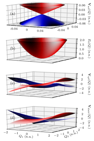
Figure 1: Potential energy surfaces in the $E\otimes e$ Jahn–Teller model around the conical intersection $Q=0$. (a) Adiabatic potential energy surfaces $V_{1}(Q)=V_{+}(Q)$ (red) and $V_{2}(Q)=V_{-}(Q)$ (blue); the two elements of the diagonal matrix $\mathbf{V}_{\mathrm{ad}}(Q)$ touch each other at the conical intersection. (b) Diagonal elements $[\mathbf{V}_{\mathrm{qd}}(Q)]_{11}=[\mathbf{V}_{\mathrm{qd}}(Q)]_{22}=[\mathbf{V}_{\mathrm{diab}}(Q)]_{11}=[\mathbf{V}_{\mathrm{diab}}(Q)]_{22}=E_{0}(Q)$ of the quasidiabatic and strictly diabatic potential energy matrices are shown together because they are all equal. (c)–(d) Off-diagonal couplings of (c) the quasidiabatic [$\mathbf{V}_{\mathrm{qd}}(Q)$] and (d) strictly diabatic [$\mathbf{V}_{\mathrm{diab}}(Q)$] potential energy matrix; the real part $\mathrm{Re}[\mathbf{V}_{i}(Q)]_{12}=\mathrm{Re}[\mathbf{V}_{i}(Q)]_{21}$ is in red, and the imaginary part $\mathrm{Im}[\mathbf{V}_{i}(Q)]_{12}=-\mathrm{Im}[\mathbf{V}_{i}(Q)]_{21}$ is in blue for $i\in\{\mathrm{qd},\mathrm{diab}\}$.

We simulated the quantum dynamics following a transition from the ground vibrational eigenstate of the electronic state of $A$ symmetry, $V_{A}(Q)=-E_{\mathrm{gap}}+E_{0}(Q)$, to the doubly degenerate states of the Jahn–Teller model by choosing the initial state as[46]

$$\tilde{\bm{\psi}}(0)=\frac{e^{-\rho(Q)^{2}/2\hbar}}{\sqrt{2\pi\hbar}}\begin{pmatrix}1\\ 1\end{pmatrix},$$ (25)

where $\tilde{\bm{\psi}}(t)=\mathbf{T}(\hat{Q})\bm{\psi}(t)$ denotes the wavepacket in the strictly diabatic representation. To obtain the initial wavepacket, we assumed an impulsive excitation, i.e., the validity of the time-dependent perturbation theory and Condon approximation during the excitation.

Among various time propagation schemes,[33, 34, 35, 36] we chose the geometric integrators[36, 38, 56] because they preserve exactly geometric properties of the exact evolution. Second-order split-operator algorithms,[37, 38, 39] including the TVT algorithm, preserve the linearity, norm, inner-product, symplecticity, stability, symmetry, and time reversibility of the exact solution.[36, 38, 56] The implicit midpoint method, like the closely related trapezoidal rule (or Crank–Nicolson) method,[84, 85] conserves, in addition, the energy. Both the split-operator and implicit midpoint methods can be symmetrically composed using various recursive or direct schemes[57, 58, 59, 36] to obtain integrators of arbitrary even orders of accuracy;[60, 61] these compositions conserve all the geometric properties conserved by the elementary methods (see Refs. 60 and 61, and Sec. S2 of the supplementary material). The composed[36, 57, 58] TVT split-operator algorithm was used to propagate the wavepacket with the separable Hamiltonians ($\hat{\mathbf{H}}_{\mathrm{diab}}$ and $\hat{\mathbf{H}}_{\text{qd-approx}}$), whereas the composed implicit midpoint method[56, 84, 85] was employed for propagations with the nonseparable Hamiltonians ($\hat{\mathbf{H}}_{\mathrm{ad}}$ and $\hat{\mathbf{H}}_{\text{qd-exact}}$). Both integrators were composed using the optimal[59] eighth-order scheme, which, when combined with a small time step $\Delta t=1/(40\omega)=0.025$ n.u., led to time discretization errors negligible to the errors due to the use of different forms of the Hamiltonian (see Sec. S3 of the supplementary material).

On a grid of infinite range and density, nonadiabatic quantum dynamics simulated using $\hat{\mathbf{H}}_{\mathrm{diab}},\hat{\mathbf{H}}_{\mathrm{ad}}$, and $\hat{\mathbf{H}}_{\text{qd-exact}}$ would be identical. Therefore, the comparison of these Hamiltonians is only meaningful for a specific finite grid; we used a uniform grid of $64\times 64$ points defined between $Q_{l}=-10$ n.u. and $Q_{l}=10$ n.u. for $l\in\{1,2\}$. Also, the favorable form of the strictly diabatic Hamiltonian allowed us to obtain the exact reference solution $\tilde{\bm{\psi}}_{\mathrm{ref}}(t):=\hat{\mathbf{U}}_{\mathrm{diab}}(t)\tilde{\bm{\psi}}(0)$ that is fully converged in both space and time: to ensure the grid convergence of the reference wavepacket, we used a grid of $128\times 128$ points defined between $Q_{l}=-10\sqrt{2}$ n.u. and $Q_{l}=10\sqrt{2}$ n.u. for $l\in\{1,2\}$. In Sec. S3 of the supplementary material, we show that both the spatial and time discretization errors of $\tilde{\bm{\psi}}_{\mathrm{ref}}(t)$ are negligible ($<10^{-10}$). In contrast, even on an infinite grid, the wavepacket $\tilde{\bm{\psi}}_{\text{qd-approx}}(t)$ would still not be exact because the residual nonadiabatic couplings are ignored. Section S3 of the supplementary material shows that even on a grid of $64\times 64$ points, the spatial discretization errors are only minor contributors to the total errors of $\tilde{\bm{\psi}}_{\text{qd-approx}}(t)$.

III Results and discussion

We compared the nonadiabatic quantum dynamics simulated using the adiabatic ($\hat{\mathbf{H}}_{\mathrm{ad}}$), exact quasidiabatic ($\hat{\mathbf{H}}_{\text{qd-exact}}$), and approximate quasidiabatic ($\hat{\mathbf{H}}_{\text{qd-approx}}$) Hamiltonians (see Sec. S4 of the supplementary material for the results obtained in the adiabatic representation without including the geometric phase). The reference quantum dynamics simulated using the strictly diabatic Hamiltonian $\hat{\mathbf{H}}_{\mathrm{diab}}$ was left out of the comparison and was only used as the benchmark because $\hat{\mathbf{H}}_{\mathrm{diab}}$ only exists, in general, when $S\rightarrow\infty$. Before comparing the wavepackets themselves, we first present a comparison of three computed observables: the power spectrum obtained by Fourier transforming the autocorrelation function $\langle\tilde{\bm{\psi}}(0)|\tilde{\bm{\psi}}(t)\rangle$ (Fig. 2), population $\mathcal{P}_{1}(t)$ of the first ($n=1$) adiabatic electronic state (Fig. 3), and position $\langle\rho(t)\rangle$ (Fig. 4). The validity of this comparison is justified because the time discretization errors of the presented observables and the time and spatial discretization errors of the reference observables are negligible (see Sec. S3 of the supplementary material).

Panels (a) of Figs. 2–4 show that none of these observables is obtained accurately with the adiabatic Hamiltonian $\hat{\mathbf{H}}_{\mathrm{ad}}$ even if the geometric phase is included: The positions and intensities of the peaks in the power spectrum are inaccurate, while the population $\mathcal{P}_{1,\mathrm{ad}}(t)$ and position $\langle\rho(t)\rangle_{\mathrm{ad}}$ deviate very rapidly from their benchmark values. In contrast, all three presented observables are computed extremely accurately if the wavepacket is propagated with the exact quasidiabatic Hamiltonian [see panels (b) of Figs. 2–4]. There is no visible difference between the observables obtained using $\hat{\mathbf{H}}_{\text{qd-exact}}$ and the benchmark observables obtained using $\hat{\mathbf{H}}_{\mathrm{diab}}$.

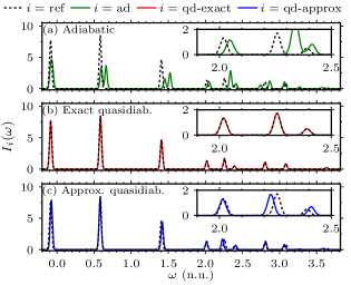
Figure 2: Power spectrum computed by Fourier transforming the autocorrelation function $\langle\tilde{\bm{\psi}}(0)|\tilde{\bm{\psi}}_{i}(t)\rangle$ of the wavepacket propagated with the (a) adiabatic ($i=\mathrm{ad}$), (b) exact quasidiabatic ($i=\textrm{qd-exact}$), or (c) approximate quasidiabatic ($i=\textrm{qd-approx}$) Hamiltonian is compared with the benchmark spectrum ($i=\mathrm{ref}$). To emulate the broadening of the peaks, the autocorrelation function was multiplied by the damping function $f(t)=\exp[-(t/t_{\mathrm{damp}})^{2}]$ with $t_{\mathrm{damp}}=80$ n.u. before the Fourier transformation. Zoomed-in versions of the spectra are presented in the insets.

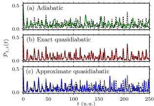
Figure 3: Time dependence of the population $\mathcal{P}_{1,i}(t):=\langle\bm{\psi}_{i}(t)|\mathbf{P}_{1}|\bm{\psi}_{i}(t)\rangle$ of the first ($n=1$) adiabatic electronic state obtained from the wavepacket propagated with the (a) adiabatic ($i=\mathrm{ad}$), (b) exact quasidiabatic ($i=\textrm{qd-exact}$), or (c) approximate quasidiabatic ($i=\textrm{qd-approx}$) Hamiltonian is compared with the benchmark population $\mathcal{P}_{1,\mathrm{ref}}(t)$; $\mathbf{P}_{n}=|n\rangle\langle n|$ is the population operator of the $n$th state. The exact norm conservation by the employed geometric integrators (see Sec. S2 of the supplementary material) implies that the population of the second electronic state is $\mathcal{P}_{2,i}(t)=1-\mathcal{P}_{1,i}(t)$ for $i\in\{\mathrm{ref},\mathrm{ad},\textrm{qd-exact},\textrm{qd-approx}\}$. Line labels are the same as in Fig. 2.

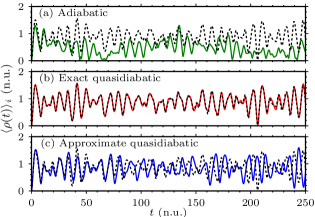
Figure 4: Time dependence of the position $\langle\rho(t)\rangle_{i}:=[\sum_{l=1}^{2}\langle\tilde{\bm{\psi}}_{i}(t)|\hat{Q}_{l}|\tilde{\bm{\psi}}_{i}(t)\rangle^{2}]^{1/2}$ obtained from the wavepacket propagated with the (a) adiabatic ($i=\mathrm{ad}$), (b) exact quasidiabatic ($i=\textrm{qd-exact}$), or (c) approximate quasidiabatic ($i=\textrm{qd-approx}$) Hamiltonian is compared with the benchmark position $\langle\rho(t)\rangle_{\mathrm{ref}}$. Line labels are the same as in Fig. 2.

Figure 2(c) shows that the spectrum obtained by Fourier transforming $\langle\tilde{\bm{\psi}}(0)|\tilde{\bm{\psi}}_{\text{qd-approx}}(t)\rangle$ is very similar to the benchmark spectrum; the differences are only clearly visible in the zoomed-in version [see inset of Fig. 2(c)]. For applications that do not require extremely precise peak positions and intensities, even the spectrum obtained using $\hat{\mathbf{H}}_{\text{qd-approx}}$ would suffice. In contrast, in panels (c) of Figs. 3 and 4, we see that both the population and position obtained with the approximate quasidiabatic Hamiltonian become inaccurate already after $t\approx 50$ n.u. For $t>50$ n.u., the population and position are described accurately only in simulations using either the exact quasidiabatic or strictly diabatic Hamiltonian. Among these Hamiltonians, however, only the exact quasidiabatic Hamiltonian exists in general unless $S\to\infty$.[41, 42]

Some observables may be accurate, even if they are computed from a poor wavepacket. In contrast, an accurate wavepacket ensures the accuracy of every observable computed from it. For a more stringent comparison between the different Hamiltonians, in Fig. 5 we, therefore, display the wavepackets $\tilde{\bm{\psi}}(t_{\mathrm{f}})$ at the final time. Whereas $\tilde{\bm{\psi}}_{\text{qd-exact}}(t)$ resembles the exact wavepacket $\tilde{\bm{\psi}}_{\mathrm{ref}}(t)$ closely and $\tilde{\bm{\psi}}_{\text{qd-approx}}(t)$ has a similar overall shape but differs in the nodal structure and other details, $\tilde{\bm{\psi}}_{\mathrm{ad}}(t)$ is completely different.

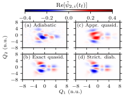
Figure 5: Accuracy of the nonadiabatic quantum dynamics simulation demonstrated by comparing the wavepackets $\tilde{\bm{\psi}}_{i}(t_{\mathrm{f}})$ at the final time $t=t_{\mathrm{f}}$ propagated with the (a) adiabatic ($i=\mathrm{ad}$), (b) exact quasidiabatic ($i=\textrm{qd-exact}$), (c) approximate quasidiabatic ($i=\textrm{qd-approx}$), or (d) strictly diabatic ($i=\mathrm{ref}$) Hamiltonian. The reference wavepacket $\tilde{\bm{\psi}}_{\mathrm{ref}}(t)$ serves as the benchmark. We only show $\mathrm{Re}[\tilde{\psi}_{2,i}(t_{\mathrm{f}})]$, i.e., the real part of the nuclear wavepacket in the second ($n=2$) electronic state of the strictly diabatic representation.

For a more quantitative comparison, we measure the error of the wavepacket $\tilde{\bm{\psi}}(t)$ using quantum fidelity[86] $\mathcal{F}(t):=|\langle\tilde{\bm{\psi}}_{\mathrm{ref}}(t)|\tilde{\bm{\psi}}(t)\rangle|^{2}$ and distance $\mathcal{D}(t):=\|\tilde{\bm{\psi}}(t)-\tilde{\bm{\psi}}_{\mathrm{ref}}(t)\|$ between $\tilde{\bm{\psi}}(t)$ and $\tilde{\bm{\psi}}_{\mathrm{ref}}(t)$, where $\|\cdot\|:=\langle\cdot|\cdot\rangle^{1/2}$ denotes the norm. The quantitative comparison, shown in Fig. 6, confirms that the quantum dynamics simulated using the exact quasidiabatic Hamiltonian is the most accurate: Quantum fidelity $\mathcal{F}_{\text{qd-exact}}(t)$ remains close to its maximal value of $\mathcal{F}_{\mathrm{max}}=1$ until the final time. Likewise, the distance $\mathcal{D}_{\text{qd-exact}}(t_{\mathrm{f}})$ at the final time is small (although nonzero). Because $\mathcal{F}_{\text{qd-exact}}(t)$ stays close to its maximal value, the nonzero distance between $\bm{\psi}_{\text{qd-exact}}(t)$ and $\bm{\psi}_{\mathrm{ref}}(t)$ is likely to be mostly due to an overall phase difference, which does not affect the local-in-time observables, such as population or position, computed from the wavepackets [as shown in panels (b) of Figs. 3 and 4]. Even the approximate quasidiabatic Hamiltonian leads to a more accurate simulation of the quantum dynamics in the vicinity of a conical intersection than the adiabatic Hamiltonian, which has the numerically problematic singularity of $\mathbf{F}_{\mathrm{ad}}(Q)$ at $Q=0$.[42] The rapid initial decrease of $\mathcal{F}_{\mathrm{ad}}(t)$ and increase of $\mathcal{D}_{\mathrm{ad}}(t)$ show that the wavepacket dynamics simulated using $\hat{\mathbf{H}}_{\mathrm{ad}}$ deviates quickly from the benchmark solution. The decay of fidelity and increase in the distance are much more gradual in the simulations with the approximate quasidiabatic Hamiltonian, although both rates of change are still much faster than the rates in the exact quasidiabatic simulation.

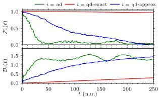
Figure 6: Time dependence of the accuracy of the wavepackets propagated with different forms of the molecular Hamiltonian. The difference between $\tilde{\bm{\psi}}_{i}(t)$ and the benchmark wavepacket $\tilde{\bm{\psi}}_{\mathrm{ref}}(t)$ is measured either with the quantum fidelity[86] $\mathcal{F}_{i}(t)=|\langle\tilde{\bm{\psi}}_{\mathrm{ref}}(t)|\tilde{\bm{\psi}}_{i}(t)\rangle|^{2}$ (top panel) or distance $\mathcal{D}_{i}(t)=\|\tilde{\bm{\psi}}_{i}(t)-\tilde{\bm{\psi}}_{\mathrm{ref}}(t)\|$ (bottom panel). Fidelity and distance were computed every hundredth time step.

IV Conclusion

We rigorously compared the suitability of different forms of the molecular Hamiltonian for simulating the nonadiabatic quantum dynamics in the vicinity of a conical intersection. This comparison was possible by taking advantage of the high-order geometric integrators and exceptional existence of the strictly diabatic Hamiltonian for the $E\otimes e$ Jahn–Teller model. The errors due to using the different forms of the molecular Hamiltonian were measured by comparing the fully converged exact reference simulation with simulations performed on a slightly sparser grid using the adiabatic, exact quasidiabatic, or approximate quasidiabatic Hamiltonian. We found that the nonadiabatic quantum dynamics simulated using the exact quasidiabatic Hamiltonian is nearly identical to the reference simulation obtained using the strictly diabatic Hamiltonian. The regularized diabatization scheme[46, 43, 82] was used for its simplicity, but the exact quasidiabatic Hamiltonian obtained through other schemes should lead to very similar and accurate results, as long as the quasidiabatization removes the conical intersection singularity, because Hamiltonian (8) is exact regardless of the quasidiabatization scheme. In contrast, the accuracy of the simulation with the approximate quasidiabatic Hamiltonian depends on the size of the neglected residual nonadiabatic couplings, and therefore, on the quasidiabatization scheme.[40]

To return to the question posed in the title, the approximate quasidiabatic Hamiltonian is appropriate if a quick solution of only moderate accuracy is required because the simple separable form of this Hamiltonian allows using more efficient time-propagation algorithms. The accuracy can be further improved by employing more sophisticated quasidiabatization schemes, which reduce the size of the neglected residual couplings. The adiabatic Hamiltonian, although exact, is not suitable for simulating quantum dynamics at a conical intersection because of the singularity of the nonadiabatic couplings there; large errors appeared since this singularity could not be described well on a finite grid. Although it was not subject of this study, the adiabatic Hamiltonian is suitable for describing quantum dynamics of a high-dimensional wavepacket moving around (i.e., not exactly through) a conical intersection, especially in on-the-fly ab initio trajectory-based simulations, in which the adiabatic Hamiltonian is obtained directly from electronic structure calculations, because the finite number of trajectories propagated in such simulations are unlikely to pass directly through conical intersection.[48, 87, 88, 89, 90] Yet, our results clearly show that the rarely used exact quasidiabatic Hamiltonian is the most suitable form of the molecular Hamiltonian for simulating nonadiabatic quantum dynamics directly at a conical intersection with high accuracy. Due to the inclusion of residual nonadiabatic couplings in the Hamiltonian, one may use any, even the simplest quasidiabatization scheme that removes the conical intersection singularity.

Supplementary material

See the supplementary material for the geometric phase effect in the $E\otimes e$ Jahn–Teller model, preservation of the geometric properties by the employed time propagation schemes, the time and spatial discretization errors of the wavepacket and presented observables, and the nonadiabatic dynamics simulated without including the geometric phase.

Data availability

The data that support the findings of this study are contained in the paper and the supplementary material.

Supplementary material for: Which form of the molecular Hamiltonian is the most suitable for simulating the nonadiabatic quantum dynamics at a conical intersection?

S1 Geometric phase effect in the $E\otimes e$ Jahn–Teller model

One way of incorporating the geometric phase effect in quantum dynamics simulations is by representing the molecular Hamiltonian using the double-valued adiabatic electronic states $|n^{\mathrm{dv}}(Q)\rangle$, which change sign upon encircling a conical intersection. The sign changes of these electronic states must be accompanied by compensating sign changes of the associated nuclear wavefunctions $\psi_{n}^{\mathrm{dv}}(Q,t)$ in order that the total molecular wavepacket $|\Psi(Q,t)\rangle$ be single-valued.[22] However, numerically representing, e.g., on a grid, a wavefunction that undergoes a sign change around a conical intersection is difficult. Another way of incorporating the geometric phase effect, according to the approach by Mead and Truhlar,[22] is to multiply the double-valued adiabatic electronic states by complex phase factors $e^{iA_{n}(Q)}$ to obtain the equivalent adiabatic states $|n(Q)\rangle=e^{iA_{n}(Q)}|n^{\mathrm{dv}}(Q)\rangle$ that are single-valued. Following previous work,[25, 26] we use the phase $A_{n}(Q)=k_{n}\phi(Q)/2$, where $k_{n}$ must be an odd integer to compensate for the sign change of $|n^{\mathrm{dv}}(Q)\rangle$ around a conical intersection.

The multiplication of $|n^{\mathrm{dv}}(Q)\rangle$ by the coordinate-dependent phase factors does not affect the diagonal adiabatic potential energy matrix because $e^{iA_{n}(Q)}$ commutes with the electronic Hamiltonian $\mathcal{H}_{\mathrm{e}}(Q)$:

$$[\mathbf{V}_{\mathrm{ad}}(Q)]_{mn} =\langle m(Q)|\mathcal{H}_{\mathrm{e}}(Q)|n(Q)\rangle=\langle m^{\mathrm{dv}}(Q)|e^{-iA_{m}(Q)}\mathcal{H}_{\mathrm{e}}(Q)e^{iA_{n}(Q)}|n^{\mathrm{dv}}(Q)\rangle$$

$$=e^{-iA_{mn}(Q)}[\mathbf{V}_{\mathrm{ad}}^{\mathrm{dv}}(Q)]_{mn}=[\mathbf{V}_{\mathrm{ad}}^{\mathrm{dv}}(Q)]_{mn},$$ (S1)

where $A_{mn}(Q):=A_{m}(Q)-A_{n}(Q)$, and the last step of Eq. (S1) holds since $[\mathbf{V}_{\mathrm{ad}}^{\mathrm{dv}}(Q)]_{mn}=\langle m^{\mathrm{dv}}(Q)|\mathcal{H}_{\mathrm{e}}(Q)|n^{\mathrm{dv}}(Q)\rangle$ is diagonal. In contrast, both the nuclear wavefunctions and nonadiabatic couplings are affected by this transformation of the adiabatic electronic states: The nuclear wavefunctions transform as $\psi_{n}(Q,t)=e^{-iA_{n}(Q)}\psi_{n}^{\mathrm{dv}}(Q,t)$ and the nonadiabatic couplings as

$$[\mathbf{F}_{\mathrm{ad}}(Q)]_{mn} =\langle m(Q)|\nabla n(Q)\rangle=\langle m^{\mathrm{dv}}(Q)|e^{-iA_{m}(Q)}\nabla e^{iA_{n}(Q)}|n^{\mathrm{dv}}(Q)\rangle$$

$$=e^{-iA_{mn}(Q)}[\langle m^{\mathrm{dv}}(Q)|\nabla n^{\mathrm{dv}}(Q)\rangle+i\nabla A_{n}(Q)\delta_{mn}]$$

$$=e^{-iA_{mn}(Q)}\{[\mathbf{F}_{\mathrm{ad}}^{\mathrm{dv}}(Q)]_{mn}+i\nabla A_{n}(Q)\delta_{mn}\}$$ (S2)

and

$$[ \mathbf{G}_{\mathrm{ad}}(Q)]_{mn}=\langle m(Q)|\nabla^{2}n(Q)\rangle=\langle m^{\mathrm{dv}}(Q)|e^{-iA_{m}(Q)}\nabla^{2}e^{iA_{n}(Q)}|n^{\mathrm{dv}}(Q)\rangle$$

$$=e^{-iA_{mn}(Q)}\{[\mathbf{G}_{\mathrm{ad}}^{\mathrm{dv}}(Q)]_{mn}+2i\nabla A_{n}(Q)[\mathbf{F}_{\mathrm{ad}}^{\mathrm{dv}}(Q)]_{mn}+[i\nabla^{2}A_{n}(Q)-\nabla A_{n}(Q)^{2}]\delta_{mn}\}.$$ (S3)

In the Jahn–Teller model, the adiabatic potential energy matrix is defined by diagonalizing the strictly diabatic potential energy matrix of the model.[54] In Refs. 54, 46, $\mathbf{V}_{\mathrm{diab}}(Q)$ is diagonalized by the transformation matrix

$$\mathbf{T}^{\mathrm{dv}}(Q)=\frac{1}{\sqrt{2}}\begin{pmatrix}e^{-i\theta(Q)}&e^{-i\theta(Q)}\\ e^{i\theta(Q)}&-e^{i\theta(Q)}\end{pmatrix},$$ (S4)

which is one out of a continuum of possible transformation matrices that diagonalize $\mathbf{V}_{\mathrm{diab}}(Q)$. This standard choice of the transformation matrix $\mathbf{T}^{\mathrm{dv}}(Q)$ yields the adiabatic electronic states

$$|1^{\mathrm{dv}}(Q)\rangle =\frac{1}{\sqrt{2}}[e^{-i\theta(Q)}|\tilde{1}\rangle+e^{i\theta(Q)}|\tilde{2}\rangle],$$

$$|2^{\mathrm{dv}}(Q)\rangle =\frac{1}{\sqrt{2}}[e^{-i\theta(Q)}|\tilde{1}\rangle-e^{i\theta(Q)}|\tilde{2}\rangle]$$ (S5)

that are coupled through the nonadiabatic vector couplings

$$\mathbf{F}_{\mathrm{ad}}^{\mathrm{dv}}(Q)=-i\nabla\theta(Q)\begin{pmatrix}0&1\\ 1&0\end{pmatrix}$$ (S6)

with vanishing diagonal elements. However, the states $|n^{\mathrm{dv}}(Q)\rangle$ are double-valued because upon encircling a conical intersection [i.e., as the polar angle $\phi(Q)$ changes from $-\pi$ to $\pi$], $\theta(Q)$ changes from $-\pi/2$ to $\pi/2$, causing $|n^{\mathrm{dv}}(Q)\rangle$ to change sign. We, therefore, multiply the double-valued states $|n^{\mathrm{dv}}(Q)\rangle$ with phase factors $e^{iA_{n}(Q)}$, where $A_{1}(Q)=-\phi(Q)/2=-\alpha(Q)$ and $A_{2}(Q)=\phi(Q)/2=\alpha(Q)$, to obtain the single-valued adiabatic electronic states

$$|1(Q)\rangle =\frac{1}{\sqrt{2}}[e^{-i\theta_{+}(Q)}|\tilde{1}\rangle+e^{i\theta_{-}(Q)}|\tilde{2}\rangle],$$

$$|2(Q)\rangle =\frac{1}{\sqrt{2}}[e^{-i\theta_{-}(Q)}|\tilde{1}\rangle-e^{i\theta_{+}(Q)}|\tilde{2}\rangle].$$ (S7)

These states are single-valued because $\theta_{+}(Q)$ changes from $-\pi$ to $\pi$ and $\theta_{-}(Q)$ starts and ends at zero as $\phi(Q)$ goes from $-\pi$ to $\pi$. Moreover, like $\mathbf{T}^{\mathrm{dv}}(Q)$, the matrix $\mathbf{T}(Q)$ [see Eq. (22) of the main text], which transforms the strictly diabatic states $|\tilde{n}\rangle$ directly into the single-valued adiabatic states $|n(Q)\rangle$, also diagonalizes $\mathbf{V}_{\mathrm{diab}}(Q)$ [into the same diagonal matrix as does $\mathbf{T}^{\mathrm{dv}}(Q)$] because overall phases of the eigenvectors can be freely chosen (and here this phase can be a function of $Q$). The two transformation matrices $\mathbf{T}(Q)$ and $\mathbf{T}^{\mathrm{dv}}(Q)$ are related by $\mathbf{T}(Q)=\mathbf{T}^{\mathrm{dv}}(Q)\mathbf{R}(Q)$, where $[\mathbf{R}(Q)]_{mn}=e^{iA_{n}(Q)}\delta_{mn}$ is the diagonal matrix that transforms the double-valued states into the single-valued states, i.e., $|n(Q)\rangle=\sum_{m=1}^{S}|m^{\mathrm{dv}}(Q)\rangle[\mathbf{R}(Q)]_{mn}$. Similarly, $\mathbf{S}(Q)=\mathbf{S}^{\mathrm{dv}}(Q)\mathbf{R}(Q)$, where the matrix

$$\mathbf{S}^{\mathrm{dv}}(Q)=\frac{1}{\sqrt{2}}\begin{pmatrix}e^{-i\alpha(Q)}&e^{-i\alpha(Q)}\\ e^{i\alpha(Q)}&-e^{i\alpha(Q)}\end{pmatrix}$$ (S8)

transforms the double-valued adiabatic states into the quasidiabatic states.

S2 Conservation of geometric properties by the time propagation schemes

In Fig. S1, we show two of the geometric properties preserved exactly by the compositions of the implicit midpoint method: the norm of the wavepacket and expectation value of energy. Among the two properties, only the norm is conserved exactly by the compositions of the split-operator algorithm. See Refs. 60 and 61 for complete analytical and numerical demonstrations of the conservation of linearity, inner-product, symplecticity, stability, symmetry, and time reversibility by symmetric compositions of the split-operator or implicit midpoint method.

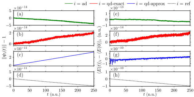
Figure S1: Exact conservation of the norm $\|\bm{\psi}_{i}(t)\|$ of the wavepacket [panels (a)–(d)] and of the expectation value $\langle E(t)\rangle_{i}$ of energy [panels (e)–(h)]. The initial value of the wavepacket norm is $\|\bm{\psi}_{i}(0)\|=1$, for $i\in\{\mathrm{ad},\textrm{qd-exact},\textrm{qd-approx},\mathrm{ref}\}$, and the initial values of the energy are $\langle E(0)\rangle_{\mathrm{ad}}=2$ n.u. and $\langle E(0)\rangle_{i}=1$ n.u., for $i\in\{\textrm{qd-exact},\textrm{qd-approx},\textrm{ref}\}$. To evaluate the expectation value of energy, the wavepackets were transformed to the same representation as the Hamiltonian: $\langle E(t)\rangle_{\mathrm{ad}}:=\langle\bm{\psi}_{\mathrm{ad}}(t)|\hat{\mathbf{H}}_{\mathrm{ad}}|\bm{\psi}_{\mathrm{ad}}(t)\rangle$, $\langle E(t)\rangle_{i}:=\langle\bm{\psi}_{i}(t)|\mathbf{S}(\hat{Q})^{\dagger}\hat{\mathbf{H}}_{i}\mathbf{S}(\hat{Q})|\bm{\psi}_{i}(t)\rangle$ for $i\in\{\textrm{qd-exact},\textrm{qd-approx}\}$, and $\langle E(t)\rangle_{\mathrm{ref}}:=\langle\tilde{\bm{\psi}}_{\mathrm{ref}}(t)|\hat{\mathbf{H}}_{\mathrm{diab}}|\tilde{\bm{\psi}}_{\mathrm{ref}}(t)\rangle$.

We used the optimal eighth-order composition[59] of the split-operator algorithm[37] to propagate the wavepacket with the separable Hamiltonians (either the approximate quasidiabatic or strictly diabatic Hamiltonian) and the optimal eighth-order composition[59] of the implicit midpoint method[56, 85] to propagate the wavepacket with the nonseparable Hamiltonians (the adiabatic or exact quasidiabatic Hamiltonian). Because exact norm and energy conservation are built into the compositions of the implicit midpoint method, these geometric properties are conserved exactly regardless of the size of the time step. Likewise, the norm is conserved exactly by the compositions of the split-operator algorithm. The apparent conservation of energy by the split-operator algorithm in Fig. S1 only results from using a very small time step. In fact, it was shown in Ref. 61 that the energy conservation by the compositions of the split-operator algorithms is not exact but follows the order of convergence of the integrator.

S3 Time and spatial discretization errors

To quantify the errors due to different forms of the molecular Hamiltonian, an exact reference solution is required. In principle, the quantum dynamics simulated using any of the three exact Hamiltonians—the strictly diabatic, exact quasidiabatic, or adiabatic Hamiltonian—can serve as a benchmark, but the wavepacket propagated with the strictly diabatic Hamiltonian is the easiest to converge in both time and space because of the separable form of this Hamiltonian. We, therefore, chose the wavepacket propagated with the strictly diabatic Hamiltonian as the benchmark. In Fig. S2, we show that both the time and spatial discretization errors of propagation with the reference Hamiltonian are negligible ($<10^{-10}$). In particular, the numerical errors of the reference wavepacket are minuscule compared to the errors due to different forms of the Hamiltonian (see Fig. 6 of the main text).

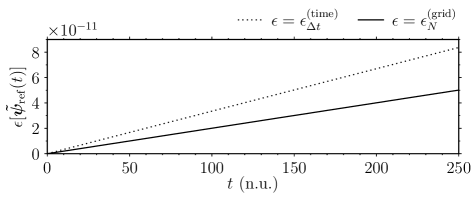
Figure S2: Time discretization errors $\epsilon_{\Delta t}^{(\mathrm{time})}[\tilde{\bm{\psi}}_{\mathrm{ref}}(t)]$ (dotted line) and spatial discretization errors $\epsilon_{N}^{(\mathrm{grid})}[\tilde{\bm{\psi}}_{\mathrm{ref}}(t)]$ (solid line) of the reference wavepacket, propagated on a grid of $128\times 128$ points ($N=128$) using the optimal eighth-order composition of the TVT split-operator algorithm with a time step of $\Delta t=0.025$ n.u. The minuscule ($<10^{-10}$) errors indicate that the reference wavepacket is converged with respect to both the time step and grid size.

We used the distance $\epsilon_{\Delta t}^{(\mathrm{time})}[\bm{\psi}(t)]:=\|\bm{\psi}^{(\Delta t,N)}(t)-\bm{\psi}^{(\Delta t/2,N)}(t)\|$ to estimate the time discretization error of $\bm{\psi}^{(\Delta t,N)}(t)$; here, $\bm{\psi}^{(\Delta t,N)}(t)$ denotes the molecular wavepacket propagated to time $t$ with the time step of $\Delta t$ on a grid of $N\times N$ points. The spatial discretization errors of $\bm{\psi}^{(\Delta t,N)}(t)$ were estimated by the distance $\epsilon_{N}^{(\mathrm{grid})}[\bm{\psi}(t)]:=\|\bm{\psi}^{(\Delta t,N)}(t)-\bm{\psi}^{(\Delta t,2N)}(t)\|$. The grid of $2N\times 2N$ points is defined to be a factor of $\sqrt{2}$ wider in each dimension compared to the grid of $N\times N$ points. Correspondingly, the grid of $2N\times 2N$ points is also a factor of $\sqrt{2}$ denser in each dimension compared to the grid of $N\times N$ points.

For an observable $A$, we measured the time discretization errors using $\epsilon_{\Delta t}^{(\mathrm{time})}(A):=|A^{(\Delta t,N)}-A^{(\Delta t/2,N)}|$ and spatial discretization errors using $\epsilon_{N}^{(\mathrm{grid})}(A):=|A^{(\Delta t,N)}-A^{(\Delta t,2N)}|$, where $A^{(\Delta t,N)}$ is the observable obtained from a simulation on a grid of $N\times N$ points using the time step $\Delta t$. Figure S3 shows that the time and spatial discretization errors of all reference observables are negligible ($<3\cdot 10^{-10}$) except for the spatial discretization errors of the population of the first ($n=1$) adiabatic electronic state, which are almost entirely due to the spatial discretization errors of the unitary transformation of the wavepacket from the strictly diabatic to the adiabatic representation. Although larger, the spatial discretization errors $\epsilon_{N}^{(\mathrm{grid})}[\mathcal{P}_{1,\mathrm{ref}}(t)]$ of the reference population are still much smaller than the differences shown in Fig. 3 of the main text; even the virtually invisible differences between $\mathcal{P}_{1,\mathrm{ref}}(t)$ and $\mathcal{P}_{1,\text{qd-exact}}(t)$ [in Fig. 3(b) of the main text] are approximately an order of magnitude greater than the spatial discretization errors of the reference population.

Figure S4 shows that the time discretization errors of the propagation with the adiabatic, exact quasidiabatic, or approximate quasidiabatic Hamiltonian are negligible (i.e., at least two orders of magnitude smaller) compared to the errors due to different forms of the Hamiltonian (cf. Fig. 6 of the main text). For the time step $\Delta t=0.025$ n.u. employed in the simulations, the composed split-operator algorithm, used for propagations with the separable approximate quasidiabatic Hamiltonian, leads to much smaller time discretization errors compared to the composed implicit midpoint method, used for propagations with the nonseparable (adiabatic or exact quasidiabatic) Hamiltonians. In both adiabatic and quasidiabatic simulations, the time discretization errors of the observables (see Fig. S5) were negligible to the errors due to the different forms of the Hamiltonian (see Figs. 2–4 of the main text).

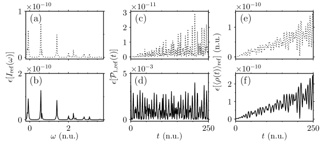
Figure S3: Time discretization errors (top) and the spatial discretization errors (bottom) of the reference observables: (a)–(b) the power spectrum, (c)–(d) population of the first ($n=1$) adiabatic electronic state, and (e)–(f) position. Line labels are the same as in Fig. S2.

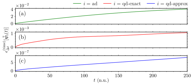
Figure S4: Time discretization errors of the wavepacket propagated with the (a) adiabatic ($i=\mathrm{ad}$), (b) exact quasidiabatic ($i=\textrm{qd-exact}$), or (c) approximate quasidiabatic ($i=\textrm{qd-approx}$) Hamiltonian. The eighth-order composition of the implicit midpoint method was used to propagate the wavepacket with either the adiabatic or exact quasidiabatic Hamiltonian. The eighth-order composition of the TVT split-operator algorithm was used to propagate the wavepacket with the approximate quasidiabatic Hamiltonian. The time step $\Delta t=0.025$ n.u. was used in all simulations.

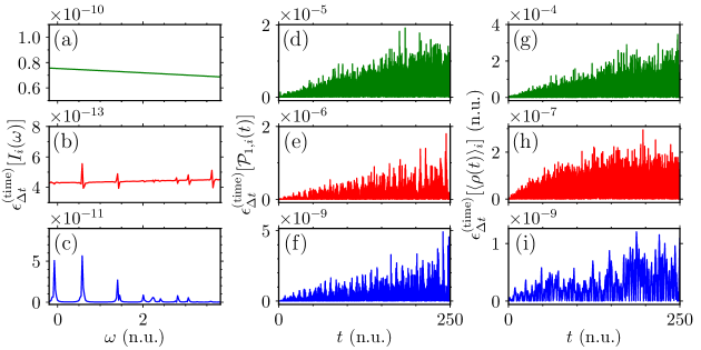
Figure S5: Time discretization errors of the power spectrum [panels (a)–(c)], population of the first ($n=1$) adiabatic electronic state [panels (d)–(f)], and position [panels (g)–(i)] obtained in the simulation with the adiabatic (top), exact quasidiabatic (middle), or approximate quasidiabatic (bottom) Hamiltonian. Line labels are the same as in Fig. S4.

The spatial discretization errors of the wavepacket propagated with either the adiabatic or exact quasidiabatic Hamiltonian are synonymous with the errors due to the different forms of the Hamiltonian. (Recall that if the nuclear wavefunctions were represented exactly, e.g., by using a grid of an infinite extent and infinite density, then the wavepackets propagated with the adiabatic or exact quasidiabatic Hamiltonian would be identical to the exact reference wavepacket.) In contrast, the error due to using the approximate quasidiabatic Hamiltonian consists of both the spatial discretization errors and errors due to neglecting the residual nonadiabatic couplings. Comparing Fig. S6 with Fig. 6 of the main text shows that neglecting the couplings is the dominant contribution.

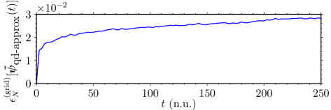
Figure S6: Spatial discretization errors of the wavepacket propagated with the approximate quasidiabatic Hamiltonian on a grid of $64\times 64$ points ($N=64$) using the optimal eighth-order composition of the TVT split-operator algorithm with a time step of $\Delta t=0.025$ n.u. The spatial discretization errors are approximately two orders of magnitude smaller than the errors (shown in Fig. 6 of the main text) due to using the approximate quasidiabatic Hamiltonian.

S4 Nonadiabatic dynamics simulated without including the geometric phase

Hamiltonian (16) of the main text is equivalent to the Hamiltonian

$$\hat{\mathbf{H}}_{\mathrm{ad}}^{\mathrm{dv}}=\mathbf{R}(\hat{Q})\hat{\mathbf{H}}_{\mathrm{ad}}\mathbf{R}(\hat{Q})^{\dagger}=\frac{1}{2M}[\hat{P}\mathbf{1}-i\hbar\mathbf{F}_{\mathrm{ad}}^{\mathrm{dv}}(\hat{Q})]^{2}+\mathbf{V}_{\mathrm{ad}}(\hat{Q})$$ (S9)

represented using the double-valued adiabatic states $|n^{\mathrm{dv}}(Q)\rangle$. However, like the electronic states themselves, the initial state $\bm{\psi}^{\mathrm{dv}}(0)=\mathbf{R}(\hat{Q})\bm{\psi}(0)$ in this representation is also double-valued. We examine the effect of neglecting the geometric phase by simulating the dynamics with one of the two branches of the double-valued state $\bm{\psi}^{\mathrm{dv}}(0)$ as the initial wavepacket.

Figure S7 shows that the power spectrum $I_{i}(\omega)$ [panel (a)], population $\mathcal{P}_{1,i}(\omega)$ [panel (b)], and position $\langle\rho(t)\rangle_{i}$ [panel (c)] obtained in the adiabatic representation without the geometric phase ($i=\text{ad-no-gp}$) are much less accurate than those obtained in the adiabatic representation in which the geometric phase is included [$i=\mathrm{ad}$, Figs. 2(a), 3(a), and 4(a) of the main text].

At the final time $t=t_{\mathrm{f}}=250$ n.u., the wavepacket propagated in the adiabatic representation does not resemble the reference wavepacket $\tilde{\bm{\psi}}_{\mathrm{ref}}(t_{\mathrm{f}})$ regardless of whether the geometric phase is included or not [compare panels (a), (b), and (c) of Fig. S8]. We, therefore, present the time dependence of various measures of the accuracy of the wavepacket $\tilde{\bm{\psi}}_{i}(t)$ propagated either with ($i=\mathrm{ad}$) or without ($i=\text{ad-no-gp}$) the geometric phase in Fig. S9. The rapid decrease of quantum fidelity$\mathcal{F}_{\text{ad-no-gp}}(t)$ [panel (a)] and rapid increase of distance $\mathcal{D}_{\text{ad-no-gp}}(t)$ [panel (b)] from the reference wavepacket show that without the geometric phase, the simulation becomes inaccurate almost immediately. The similarly sharp changes in quantum fidelity $\mathcal{F}(t)$ and distance $\mathcal{D}(t)$ between the two wavepackets $\tilde{\bm{\psi}}_{i}(t)$ propagated either with ($i=\mathrm{ad}$) or without ($i=\text{ad-no-gp}$) the geometric phase (shown in the right-hand panels of Fig. S9) confirms that ignoring the geometric phase is responsible for the rapid decrease in the accuracy of $\tilde{\bm{\psi}}_{\text{ad-no-gp}}(t)$.

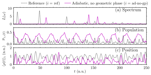
Figure S7: (a) Power spectrum, (b) population, and (c) position obtained without including the geometric phase in the adiabatic representation ($i=\textrm{ad-no-gp}$) are compared with the reference observables obtained with the strictly diabatic Hamiltonian. Panels (a), (b), and (c) are analogous to Figs. 2(a), 3(a), and 4(a) of the main text, respectively.

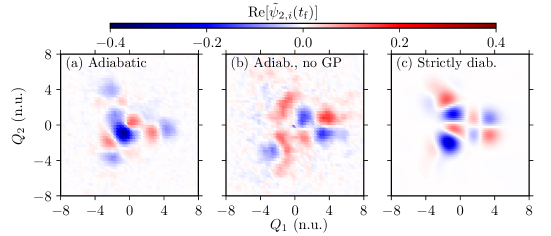
Figure S8: Effect of neglecting the geometric phase demonstrated by comparing the wavepackets $\tilde{\bm{\psi}}_{i}(t_{\mathrm{f}})$ at the final time, propagated in the adiabatic representation with [$i=\mathrm{ad}$, panel (a)] or without [$i=\textrm{ad-no-gp}$, panel (b)] the geometric phase. The benchmark wavepacket $\tilde{\bm{\psi}}_{\mathrm{ref}}(t_{\mathrm{f}})$ propagated in the strictly diabatic representation is shown as a reference in panel (c).

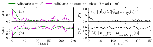
Figure S9: Time dependence of the accuracy of the nonadiabatic dynamics simulated in the adiabatic representation either with ($i=\mathrm{ad}$) or without ($i=\textrm{ad-no-gp}$) the geometric phase is measured by (a) the quantum fidelity $\mathcal{F}_{i}(t)$ and (b) distance $\mathcal{D}_{i}(t)$ between $\tilde{\bm{\psi}}_{i}(t)$ and the benchmark wavepacket $\tilde{\bm{\psi}}_{\mathrm{ref}}(t)$. The importance of the geometric phase is measured more directly by (c) the quantum fidelity $\mathcal{F}(t)=|\langle\tilde{\bm{\psi}}_{\mathrm{ad}}(t)|\tilde{\bm{\psi}}_{\textrm{ad-no-gp}}(t)\rangle|^{2}$ and (d) distance $\mathcal{D}(t)=\|\tilde{\bm{\psi}}_{\mathrm{ad}}(t)-\tilde{\bm{\psi}}_{\textrm{ad-no-gp}}(t)\|$ between the wavepackets propagated in the adiabatic representation either with ($i=\mathrm{ad}$) or without ($i=\textrm{ad-no-gp}$) the geometric phase.

References

- Teller [1937] E. Teller, J. Phys. Chem. 41, 109 (1937).
- Förster [1970] T. Förster, Pure Appl. Chem 24, 443 (1970).
- Herzberg and Longuet-Higgins [1963] G. Herzberg and H. Longuet-Higgins, Faraday Discuss. 35, 77 (1963).
- Zimmerman [1966] H. E. Zimmerman, J. Am. Chem. Soc. 88, 1566 (1966).
- Koppel, Domcke, and Cederbaum [1984] H. Koppel, W. Domcke, and L. S. Cederbaum, Adv. Chem. Phys. 57, 59 (1984).
- Yarkony [1990] D. R. Yarkony, J. Chem. Phys. 92, 2457 (1990).
- Atchity, Xantheas, and Ruedenberg [1991] G. J. Atchity, S. S. Xantheas, and K. Ruedenberg, J. Chem. Phys. 95, 1862 (1991).
- Bernardi et al. [1990] F. Bernardi, S. De, M. Olivucci, and M. A. Robb, J. Am. Chem. Soc. 112, 1737 (1990).
- Klessinger and Michl [1995] M. Klessinger and J. Michl, Excited states and photochemistry of organic molecules (VCH publishers, 1995).
- Baer [2006] M. Baer, Beyond Born-Oppenheimer: Electronic Nonadiabatic Coupling Terms and Conical Intersections, 1st ed. (Wiley, 2006).
- Domcke and Yarkony [2012] W. Domcke and D. R. Yarkony, Annu. Rev. Phys. Chem. 63, 325 (2012).
- Nakamura [2012] H. Nakamura, Nonadiabatic Transition: Concepts, Basic Theories and Applications, 2nd ed. (World Scientific Publishing Company, 2012).
- Takatsuka et al. [2015] K. Takatsuka, T. Yonehara, K. Hanasaki, and Y. Arasaki, Chemical Theory Beyond the Born-Oppenheimer Paradigm: Nonadiabatic Electronic and Nuclear Dynamics in Chemical Reactions (World Scientific, Singapore, 2015).
- Bircher et al. [2017] M. P. Bircher, E. Liberatore, N. J. Browning, S. Brickel, C. Hofmann, A. Patoz, O. T. Unke, T. Zimmermann, M. Chergui, P. Hamm, U. Keller, M. Meuwly, H. J. Woerner, J. Vaníček, and U. Rothlisberger, Struct. Dyn. 4, 061510 (2017).
- Shin and Metiu [1995] S. Shin and H. Metiu, J. Chem. Phys. 102, 9285 (1995).
- Albert, Kaiser, and Engel [2016] J. Albert, D. Kaiser, and V. Engel, J. Chem. Phys. 144, 171103 (2016).
- Abedi, Maitra, and Gross [2010] A. Abedi, N. T. Maitra, and E. K. Gross, Phys. Rev. Lett. 105, 123002 (2010).
- Cederbaum [2008] L. S. Cederbaum, J. Chem. Phys. 128, 124101 (2008).
- Worth and Cederbaum [2004] G. A. Worth and L. S. Cederbaum, Annu. Rev. Phys. Chem. 55, 127 (2004).
- Cederbaum [2004] L. S. Cederbaum, in Conical intersections: electronic structure, dynamics and spectroscopy (World Scientific, 2004) pp. 3–40.
- Longuet-Higgins et al. [1958] H. C. Longuet-Higgins, U. Öpik, M. H. L. Pryce, and R. Sack, Proc. Royal Soc. A (London) 244, 1 (1958).
- Mead and Truhlar [1979] C. A. Mead and D. G. Truhlar, J. Chem. Phys. 70, 2284 (1979).
- Berry [1984] M. V. Berry, Proc. Roy. Soc. London Sect. A 392, 45 (1984).
- Mead [1992] C. A. Mead, Rev. Mod. Phys. 64, 51 (1992).
- Kendrick [2000] B. K. Kendrick, J. Chem. Phys. 112, 5679 (2000).
- Juanes-Marcos and Althorpe [2005] J. C. Juanes-Marcos and S. C. Althorpe, J. Chem. Phys. 122, 204324 (2005).
- Malbon et al. [2016] C. L. Malbon, X. Zhu, H. Guo, and D. R. Yarkony, J. Chem. Phys. 145, 234111 (2016).
- Xie et al. [2019] C. Xie, C. L. Malbon, H. Guo, and D. R. Yarkony, Acc. Chem. Res. 52, 501 (2019).
- Xie, Yarkony, and Guo [2017] C. Xie, D. R. Yarkony, and H. Guo, Phys. Rev. A 95, 022104 (2017).
- Ryabinkin, Joubert-Doriol, and Izmailov [2017] I. G. Ryabinkin, L. Joubert-Doriol, and A. F. Izmailov, Acc. Chem. Res. 50, 1785 (2017).
- Joubert-Doriol, Ryabinkin, and Izmaylov [2013] L. Joubert-Doriol, I. G. Ryabinkin, and A. F. Izmaylov, J. Chem. Phys. 139, 234103 (2013).
- Schön and Köppel [1995] J. Schön and H. Köppel, J. Chem. Phys. 103, 9292 (1995).
- Leforestier et al. [1991] C. Leforestier, R. H. Bisseling, C. Cerjan, M. D. Feit, R. Friesner, A. Guldberg, A. Hammerich, G. Jolicard, W. Karrlein, H.-D. Meyer, N. Lipkin, O. Roncero, and R. Kosloff, J. Comp. Phys. 94, 59 (1991).
- Tal-Ezer and Kosloff [1984] H. Tal-Ezer and R. Kosloff, J. Chem. Phys. 81, 3967 (1984).
- Park and Light [1986] T. J. Park and J. C. Light, J. Chem. Phys. 85, 5870 (1986).
- Hairer, Lubich, and Wanner [2006] E. Hairer, C. Lubich, and G. Wanner, Geometric Numerical Integration: Structure-Preserving Algorithms for Ordinary Differential Equations (Springer Berlin Heidelberg New York, 2006).
- Feit, Fleck, and Steiger [1982] M. D. Feit, J. A. Fleck, Jr., and A. Steiger, J. Comp. Phys. 47, 412 (1982).
- Lubich [2008] C. Lubich, From Quantum to Classical Molecular Dynamics: Reduced Models and Numerical Analysis, 12th ed. (European Mathematical Society, Zürich, 2008).
- Tannor [2007] D. J. Tannor, Introduction to Quantum Mechanics: A Time-Dependent Perspective (University Science Books, Sausalito, 2007).
- Choi and Vaníček [2020] S. Choi and J. Vaníček, “How important are the residual nonadiabatic couplings for the accurate simulation of the nonadiabatic quantum dynamics?” (2020), submitted.
- Mead and Truhlar [1982] C. A. Mead and D. G. Truhlar, J. Chem. Phys. 77, 6090 (1982).
- Pacher et al. [1989] T. Pacher, C. A. Mead, L. S. Cederbaum, and H. Köppel, J. Chem. Phys. 91, 7057 (1989).
- Köppel, Gronki, and Mahapatra [2001] H. Köppel, J. Gronki, and S. Mahapatra, J. Chem. Phys. 115, 2377 (2001).
- Pacher, Cederbaum, and Köppel [1988] T. Pacher, L. S. Cederbaum, and H. Köppel, J. Chem. Phys. 89, 7367 (1988).
- Gadéa and Pélissier [1990] F. X. Gadéa and M. Pélissier, J. Chem. Phys. 93, 545 (1990).
- Thiel and Köppel [1999] A. Thiel and H. Köppel, J. Chem. Phys. 110, 9371 (1999).
- Viel et al. [2004] A. Viel, R. P. Krawczyk, U. Manthe, and W. Domcke, J. Chem. Phys. 120, 11000 (2004).
- Ben-Nun, Quenneville, and Martínez [2000] M. Ben-Nun, J. Quenneville, and T. J. Martínez, J. Phys. Chem. A 104, 5161 (2000).
- Ibele and Curchod [2020] L. M. Ibele and B. F. Curchod, Phys. Chem. Chem. Phys. 22, 15183 (2020).
- Mandal, Yamijala, and Huo [2018] A. Mandal, S. S. Yamijala, and P. Huo, J. Chem. Theory Comput. 14, 1828 (2018).
- Zhou, Mandal, and Huo [2019] W. Zhou, A. Mandal, and P. Huo, J. Phys. Chem. Lett. 10, 7062 (2019).
- Guo and Yarkony [2016] H. Guo and D. R. Yarkony, Phys. Chem. Chem. Phys. 18, 26335 (2016).
- Xie et al. [2016] C. Xie, J. Ma, X. Zhu, D. R. Yarkony, D. Xie, and H. Guo, J. Am. Chem. Soc. 138, 7828 (2016).
- Bersuker and Polinger [2012] I. B. Bersuker and V. Z. Polinger, Vibronic interactions in molecules and crystals, Vol. 49 (Springer Science & Business Media, 2012).
- Bersuker [2001] I. B. Bersuker, Chem. Rev. 101, 1067 (2001).
- Leimkuhler and Reich [2004] B. Leimkuhler and S. Reich, Simulating Hamiltonian Dynamics (Cambridge University Press, 2004).
- Suzuki [1990] M. Suzuki, Phys. Lett. A 146, 319 (1990).
- Yoshida [1990] H. Yoshida, Phys. Lett. A 150, 262 (1990).
- Kahan and Li [1997] W. Kahan and R.-C. Li, Math. Comput. 66, 1089 (1997).
- Choi and Vaníček [2019] S. Choi and J. Vaníček, J. Chem. Phys. 150, 204112 (2019).
- Roulet, Choi, and Vaníček [2019] J. Roulet, S. Choi, and J. Vaníček, J. Chem. Phys. 150, 204113 (2019).
- Born and Huang [1954] M. Born and K. Huang, Dynamical theory of crystal lattices (Oxford University Press, London, 1954).
- Ballhausen and Hansen [1972] C. Ballhausen and A. E. Hansen, Annu. Rev. Phys. Chem. 23, 15 (1972).
- Yarkony [1996] D. R. Yarkony, Rev. Mod. Phys. 68, 985 (1996).
- Köppel [2004a] H. Köppel, in Conical intersections: electronic structure, dynamics and spectroscopy (World Scientific, 2004) pp. 175–204.
- Yarkony [2004] D. R. Yarkony, in Conical intersections: electronic structure, dynamics and spectroscopy (World Scientific, 2004) pp. 41–127.
- Pacher, Köppel, and Cederbaum [1991] T. Pacher, H. Köppel, and L. S. Cederbaum, J. Chem. Phys. 95, 6668 (1991).
- Neville, Seidu, and Schuurman [2020] S. P. Neville, I. Seidu, and M. S. Schuurman, J. Chem. Phys. 152, 114110 (2020).
- Domcke and Woywod [1993] W. Domcke and C. Woywod, Chem. Phys. Lett. 216, 362 (1993).
- Baer [1975] M. Baer, Chem. Phys. Lett. 35, 112 (1975).
- Das et al. [2011] A. Das, D. Mukhopadhyay, S. Adhikari, and M. Baer, Chem. Phys. Lett. 517, 92 (2011).
- Richings and Worth [2015] G. W. Richings and G. A. Worth, J. Phys. Chem. A 119, 12457 (2015).
- Sadygov and Yarkony [1998] R. G. Sadygov and D. R. Yarkony, J. Chem. Phys. 109, 20 (1998).
- Esry and Sadeghpour [2003] B. D. Esry and H. R. Sadeghpour, Phys. Rev. A 68, 042706 (2003).
- Mulliken [1952] R. S. Mulliken, J. Am. Chem. Soc. 74, 811 (1952).
- Hush [1967] N. Hush, Prog. Inorg. Chem 8, 12 (1967).
- Cave and Newton [1997] R. J. Cave and M. D. Newton, J. Chem. Phys. 106, 9213 (1997).
- Werner and Meyer [1981] H.-J. Werner and W. Meyer, J. Chem. Phys. 74, 5802 (1981).
- Yarkony [1998] D. R. Yarkony, J. Phys. Chem. A 102, 8073 (1998).
- Hirsch, Buenker, and Petrongolo [1990] G. Hirsch, R. J. Buenker, and C. Petrongolo, Mol. Phys. 70, 835 (1990).
- Perić, Peyerimhoff, and Buenker [1990] M. Perić, S. D. Peyerimhoff, and R. J. Buenker, Mol. Phys. 71, 693 (1990).
- Köppel and Schubert [2006] H. Köppel and B. Schubert, Mol. Phys. 104, 1069 (2006).
- Köppel [2004b] H. Köppel, Faraday Discuss. 127, 35 (2004b).
- Crank and Nicolson [1947] J. Crank and P. Nicolson, Math. Proc. Camb. Phil. Soc. 43, 50 (1947).
- McCullough and Wyatt [1971] E. A. McCullough, Jr. and R. E. Wyatt, J. Chem. Phys. 54, 3578 (1971).
- Peres [1984] A. Peres, Phys. Rev. A 30, 1610 (1984).
- Curchod and Martínez [2018] B. F. E. Curchod and T. J. Martínez, Chem. Rev. 118, 3305 (2018).
- Lasorne et al. [2006] B. Lasorne, M. J. Bearpark, M. A. Robb, and G. A. Worth, Chem. Phys. Lett. 432, 604 (2006).
- Worth, Robb, and Burghardt [2004] G. A. Worth, M. A. Robb, and I. Burghardt, Faraday Discuss. 127, 307 (2004).
- Saita and Shalashilin [2012] K. Saita and D. V. Shalashilin, J. Chem. Phys. 137, 22A506 (2012).