On Scalar and Ricci Curvatures

On Scalar and Ricci Curvatures

Gerard BESSON and Sylvestre GALLOT

G. Besson and S. Gallot

CNRS-Université Grenoble Alpes, Institut Fourier, CS 40700, 38058 Grenoble cedex 09, France g.besson@univ-grenoble-alpes.fr, sylvestre.gallot@univ-grenoble-alpes.fr

Received October 19, 2020, in final form April 05, 2021; Published online May 01, 2021

The purpose of this report is to acknowledge the influence of M. Gromov’s vision of geometry on our own works. It is two-fold: in the first part we aim at describing some results, in dimension $3$, around the question: which open $3$-manifolds carry a complete Riemannian metric of positive or non negative scalar curvature? In the second part we look for weak forms of the notion of “lower bounds of the Ricci curvature” on non necessarily smooth metric measure spaces. We describe recent results some of which are already posted in [arXiv:1712.08386] where we proposed to use the volume entropy. We also attempt to give a new synthetic version of Ricci curvature bounded below using Bishop–Gromov’s inequality.

scalar curvature; Ricci curvature; Whitehead 3-manifolds; infinite connected sums; Ricci flow; synthetic Ricci curvature; metric spaces; Bishop–Gromov inequality; Gromov-hyperbolic spaces; hyperbolic groups; Busemann spaces; CAT(0)-spaces

51K10; 53C23; 53C21; 53E20; 57K30

Happy Birthday Misha

1 Introduction

The purpose of this text is to acknowledge the influence of M. Gromov’s vision of geometry on our own works. It started in the early 80’s with the french version of the so-called “green book” [31]. We then discovered some of his previous articles and followed his progression in the new realm that he was building.

The following text is two-fold. In the first part (Section 2) we aim at describing some results, in dimension $3$, around the question: which open $3$-manifolds carry a complete Riemannian metric of positive or non negative scalar curvature? The influential article is the joint work by M. Gromov and B. Lawson [35] and, in particular, the beautiful Chapter 10 where the relation between a $3$-manifold carrying a metric with positive scalar curvature and the stable minimal surfaces that it contains is subtly exploited. We focus on two types of $3$-manifolds: the so-called decomposable $3$-manifolds and the contractible $3$-manifolds. For the first family the results are extensions to open $3$-manifolds of a corollary of Perelman’s works asserting that a closed $3$-manifold has a metric of positive scalar curvature if and only if it is a connected sum of spherical manifolds (see Section 2.2 for the details). The second part of this section is about the family of contractible open $3$-manifolds, which is very rich, and found its origin in early works by J.H.C. Whitehead (see Section 2.1). The goal here would be to show that only $\mathbb{R}^{3}$ carries a complete metric of positive scalar curvature. It is not yet achieved but the results are already quite striking and strongly influenced by the article [35]. In both parts the results culminate with works by Jian Wang.

So far we have been looking for smooth metrics on smooth Riemannian manifolds. In view of some recent developments we could search for non smooth metrics on these contractible spaces, for example. These raises quite a few exciting questions which are asked at the end of Section 2.

In the second part (Section 3) we are indeed interested in non necessarily smooth metric measure spaces. The underlying philosophy founds its origin as far as in the article [3]. However, most of the results that are described are proved in the preprint [4] and some others will be in a forthcoming article, by the same authors, to be posted soon. In this Section 3 we look for weak forms of lower bounds of the Ricci curvature. This already exists, for example curvature-dimension conditions à la Bakry–Emery, the so-called CD(K,N) condition where $K$ stands for a lower bound of the Ricci curvature and $N$ for an upper bound on the dimension. The original version was about operators (or semi-groups generated by an operator), typically the Laplacian of a Riemannian manifold and it somehow used a weak version of Bochner formula as a definition of a lower bound on the Ricci curvature. It was then extended, using measure transportation, to what is now called synthetic Ricci curvature by Lott–Villani and Sturm (see Section 3.1.2($b$)). In [4] we propose to use an upper bound on the volume entropy as a replacement to a lower bound on the Ricci curvature. The volume entropy of a Riemannian manifold is related to the asymptotic growth of the volume of balls of radius $R$ around a point in its universal cover and its definition is given in Definition 3.6.

By Bishop’s comparison theorem it is easy to show that, if the Ricci curvature of a Riemannian metric $g$ satisfies that $\operatorname{Ric}(g)\geq-(n-1)\kappa g$ where $\kappa$ is a non negative real number, then the entropy is bounded above by $(n-1)\sqrt{\kappa}$. Hence an upper bound on the entropy could serve as a (very) weak version of a lower bound on the Ricci curvature. Now, a lower bound on the Ricci curvature, in the Riemannian case, implies the Bishop–Gromov’s comparison theorem which is an easy modification of Bishop’s original result which has amazing consequences. This is the case also with (some of) the synthetic version of the Ricci curvature and we show in [4] that it is also the case, at least in a weaker form, with the upper bound on the volume entropy (together with other natural assumptions) applied to metric measure spaces. In Section 3 we decided to use this consequence as a definition of the expression “Ricci curvature bounded below”, yet another version in the spirit of Bakry–Emery $\operatorname{CD}(K,N)$ somehow but on the geometric side, where Bochner formula is replaced by Bishop–Gromov’s comparison. We develop both this approach and the entropy approach applied to metric measure spaces in Section 3 and go as far as describing versions of the celebrated Margulis lemma and its consequences on proving finiteness and compactness results. The reader is referred to this section for precise statements.

It would be clear by now that Misha’s works has had a great influence on ours and we are greatly indebted to him for the exchanges and discussions that we had along these years. We also owe a lot to our former advisor Marcel Berger who passed away on October 15, 2016 and his teaching remains in our memory. He admired Gromov, as we do, and right after Misha settled in France, at any questions from us he would answer “ask Gromov, he knows!”

2 Scalar curvature: on some works of Schoen–Yau,
Gromov–Lawson and Jian Wang

2.1 Introduction

This section is a short account of some recent results concerning the existence of metrics with non negative scalar curvature on some $3$-manifolds. The starting point of our interest is the “proof” of the Poincaré conjecture given in 1934 by J.H.C. Whitehead in the article [71]. Roughly speaking the scheme is the following (see here):

• Let $X$ be a simply connected closed $3$-manifolds then, for any point $p\in X$, $X\setminus\{p\}$ is contractible (by simple considerations left to the reader).

• The only contractible $3$-manifolds is $\mathbb{R}^{3}$.

• The one-point compactification of $\mathbb{R}^{3}$ is $\mathbb{S}^{3}$.

In 1935 he realised that the second step was wrong (see [72]) and constructed in [73] the first contractible $3$-manifold which is not homeomorphic to $\mathbb{R}^{3}$, the now-called Whitehead manifold which we shall denote by $\rm Wh$.

Let us dream of a version of the Poincaré conjecture for open manifolds. What could it be? Well, an open manifold which has the same homotopy as $\mathbb{R}^{3}$, that is which is contractible, is homeomorphic to $\mathbb{R}^{3}$! The Whitehead manifold is a counter-example to this statement and a non compact version of the Poincaré conjecture is not true! However, the discovery of $3$-manifolds which are contractible but not homeomorphic to $\mathbb{R}^{3}$, such as the Whitehead manifold, opened a wide playground for topologists and geometers. Mistakes could be useful, indeed a similar experience happened to Poincaré too.

The Whitehead manifold $\rm Wh$ is an open subset of $\mathbb{S}^{3}$ whose complement is a closed set, called the Whitehead continuum, which looks locally like a product of an interval with a Cantor set. It is easily seen, by construction, that $\rm Wh$ is contractible and the fact that it is not homeomorphic to $\mathbb{R}^{3}$ follows from the fact that it is not simply-connected at infinity (see a definition in Section 2.3). Such manifolds, not homeomorphic to $\mathbb{R}^{3}$ but nevertheless contractible, turn out to be plentiful, as was shown by McMillan (see [52]). In fact there exist uncountably many such manifolds whereas there are only a countable family of closed topological manifolds. Many other nice properties can be proved and the reader is referred to the literature.

Let us come back to Poincaré’s conjecture. In the Clay–Perelman conference, in the lecture entitled “What is a Manifold”, given at I.H.P. in 2011, Misha Gromov, talking about the Poincaré conjecture says “and so what?” (see here, at time 13:30). This is typical of Misha’s point of view, an information on one object, here being able to recognise the $3$-sphere only, is nice but does not contain enough knowledge. A general picture is more important, even if it is incomplete, or, in other words, getting statistical informations is more useful than knowing a single value. This general picture was given by W. Thurston in the 70’s and is known as Thurston’s geometrisation conjecture (see [66] and the post-Perelman literature). It is a conjectural description of all closed $3$-manifolds and the way to build or decompose them nicely, which yields the Poincaré conjecture as a corollary. The picture is so clear and so nice that the attempts to publish counter-examples to the Poincaré conjecture (almost) stopped. In any case it took then less than 30 years to get G. Perelman’s proof of Thurston’s conjecture (see [54, 55, 56]) developing a technique introduced by R. Hamilton in [40].

The beautiful idea of Thurston is to decompose the closed $3$-manifolds into pieces carrying each a very specific Riemannian geometry, like the case of closed surfaces which are either spherical, flat or hyperbolic but with more (in fact 8) possibilities. Now, what could be a geometrisation conjecture for open $3$-manifolds? There is little hope to be able to state a reasonable conjecture. For example, the starting point of Thurston’s geometrisation conjecture are the Kneser–Milnor and the Jaco–Shalen and Johannson decompositions of closed $3$-manifolds none of which is true for open manifolds (see [61] and [50]). Therefore, the only sensible thing to do is to work out examples and this is the purpose of the next two sections. We shall describe two extremely different families of open $3$-manifolds and explore their Riemannian geometry with an emphasis on the scalar curvature.

2.2 Decomposable 3-manifolds

This is a family of $3$-manifolds that generalises connected sums. More precisely let $\mathcal{X}$ be a class of orientable closed $3$-manifolds. A manifold $M$ is a (possibly infinite) connected sum of members of $\mathcal{X}$ if there exists a locally finite graph $G$ (or simply a locally finite tree $T$) and a map $v\mapsto X_{v}$ which associates to each vertex of $G$ a copy of some manifold in $\mathcal{X}$ such that, by removing from each $X_{v}$ as many $3$-balls as edges incident to $v$ and gluing the thus punctured $X_{v}$’s to each other along the edges of $G$, one obtains a $3$-manifold diffeomorphic to $M$. Precise definitions and several useful comments may be found in [2].

We now shall consider Riemannian manifolds with positive scalar curvature. This class has been extensively studied since the works of A. Lichnérowicz, R. Schoen, S.-T. Yau, M. Gromov, B. Lawson and others (see, e.g., the survey articles [30, 58]).

Let $(M,g)$ be a Riemannian manifold. We denote by $\textrm{Scal}_{\mathrm{min}}(g)$ the infimum of the scalar curvature of $g$ and we say that $g$ has uniformly positive scalar curvature if $\textrm{Scal}_{\mathrm{min}}(g)>0$. If $M$ is compact then this amounts to saying that $g$ should have positive scalar curvature at each point of $M$.

A $3$-manifold is spherical if it admits a metric of positive constant sectional curvature. M. Gromov and B. Lawson [34] have shown that any compact, orientable $3$-manifold which is a connected sum of orientable spherical manifolds and copies of $S^{2}\times S^{1}$ carries a metric of positive scalar curvature. G. Perelman [55], completing pioneering work of Schoen–Yau [59] and Gromov–Lawson [35], proved the converse.

As mentioned before we are mostly interested in the non compact case. We say that a Riemannian metric $g$ on $M$ has bounded geometry if it has bounded sectional curvature and injectivity radius bounded away from zero. It follows from the Gromov–Lawson construction that, if the $3$-manifold $M$ is a (possibly infinite) connected sum of spherical manifolds, taken in a finite list (see the statement below), and of copies of $S^{2}\times S^{1}$, then $M$ admits a complete metric of bounded geometry and uniformly positive scalar curvature. The following theorem by L. Bessières, G. Besson and S. Maillot shows that the converse holds, generalising Perelman’s theorem:

Theorem 2.1 ([2]).

Let $M$ be a connected, orientable $3$–manifold which carries a complete Riemannian metric of bounded geometry and uniformly positive scalar curvature. Then there is a finite collection $\mathcal{X}$ of spherical manifolds such that $M$ is a connected sum of copies of $S^{2}\times S^{1}$ and members of $\mathcal{X}$.

The proof relies on an extension of the Ricci flow with surgery, called a surgical solution, that is constructed in the same article [2]. It is not the purpose of this text to give the details of this construction and the interested reader is referred to [2]. Let us though emphasise that the bounded geometry assumption is the necessary requirement in order to trigger this new Ricci flow and to ensure its existence for all time. The finiteness of the class $\mathcal{X}$ is a consequence of the combination of the lower bound on the injectivity radius and of the uniformly positive scalar curvature. More precisely, let us normalise the metric so that $\textrm{Scal}_{\mathrm{min}}=6$. The spherical manifolds are quotients of the $3$-sphere with a constant sectional curvature metric and with this normalisation this constant is equal to $1$; there are infinitely many of them, the lens spaces for example, and their injectivity radius goes to zero. Hence, a lower bound on the injectivity radius combined with the lower bound on $\textrm{Scal}_{\mathrm{min}}$ reduces $\mathcal{X}$ to a finite set.

The article [12] contains results closely related to Theorem 2.1. Precisely, Theorem 5.1 in [12] has the same conclusion than 2.1 without the assumption that the metric has bounded geometry but with the assumption that $M$ has a finitely generated fundamental group. Notice that, in Theorem 2.1, if $M$ is a connected sum of an infinite number of copies of members of $\mathcal{X}$ (different from $\mathbb{S}^{3}$), its fundamental group is not finitely generated. An interesting point is that the proof described in [12] relies on $K$-theory and hence is completely different from the proof of Theorem 2.1. Somehow $K$-theory has to do with the Dirac operator and the relation between the square of the Dirac operator and the scalar curvature is encoded in the Bochner–Lichnérowicz–Weitzenbock formula (see [35, equation (2.14), p. 112]).

Recently Jian Wang announced the proof of the following result which improves both Theorem 2.1 and the result in [12].

Theorem 2.2 ([70]).

A complete connected orientable $3$-manifold of uniformly positive scalar curvature is homeomorphic to a $($possibly infinite$)$ connected sum of spherical $3$-manifolds and copies of $S^{2}\times S^{1}$.

The progress here is that there is neither the assumption that $g$ has bounded geometry nor that the fundamental group of $M$ is finitely generated. The proof is yet another one; it uses the case of closed manifolds, proved by G. Perelman [56], but neither a version of the Ricci flow for open manifolds nor $K$-theory. The theory of minimal surfaces and the special relations between stable minimal surfaces and the scalar curvature of the ambient metric in dimension $3$ is essential.

2.3 Contractible $\mathbf{3}$-manifolds

We now come to the second series of examples, namely the contractible open $3$-manifolds which are not homeomorphic to $\mathbb{R}^{3}$. They are somehow opposite to the class of decomposable manifolds in the sense that they are homotopically trivial and their topology is hidden in their structure at infinity. Let us recall the construction of the main example, the Whitehead manifold. We start with the Whitehead link which is a link with two components illustrated in Figure 1 below in two different ways. Notice that this link is symmetric; this means that there is an isotopy of the ambient space which reverses the roles played by the black and red curves.

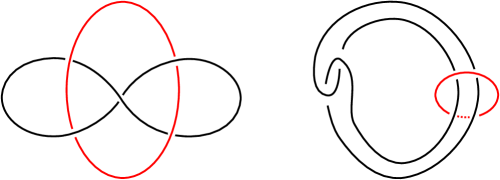
Figure 1: Whitehead link.

For a closed solid torus $T$ we define the notion of a meridian curve. A meridian $\gamma\subset\partial T$ is an embedded circle which is nullhomotopic in $T$ but not contractible in $\partial T$. On Figure 2 the red curve is a meridian.

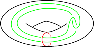
Figure 2: $T_{2}\subset T_{1}$.

Now we choose a closed unknotted solid torus $T_{1}\subset\mathbb{S}^{3}$. It is well known that the complement of $T_{1}$ in $\mathbb{S}^{3}$ is another solid torus (this time open). We then embed a second solid torus $T_{2}$ inside $T_{1}$ as a tubular neighbourhood of the green curve. The green and red curves form a Whitehead link. This is the basic pattern of the construction which we will repeat infinitely many times. Precisely, $T_{2}$ is also an unknotted solid torus in $\mathbb{S}^{3}$ and we then embed $T_{3}$ inside $T_{2}$ in the same way as $T_{2}$ lies in $T_{1}$. We do this infinitely many times and define $T_{\infty}:=\cap_{k=1}^{\infty}T_{k}$ which is a closed subset of $\mathbb{S}^{3}$ called the Whitehead continuum. The Whitehead manifold is then defined as $Wh:=\mathbb{S}^{3}\setminus T_{\infty}$ which is an open manifold (i.e., a non compact manifold without boundary), an open subset of $\mathbb{S}^{3}$ (hence of $\mathbb{R}^{3}$ too).

The symmetry of the Whitehead link allows to give an alternative definition. Note that each $T_{k}$ is an unknotted solid torus in $\mathbb{S}^{3}$, it is however knotted in $T_{k-1}$; we recall that this means that no isotopy of $T_{k-1}$ can unknot $T_{k}$. Nevertheless $T_{k}$ is homotopically trivial in $T_{k-1}$. Being unknotted in $\mathbb{S}^{3}$, the complement of $T_{k}$ is a (open) solid torus $N_{k}$. The manifold $\rm Wh$ can then be defined as the increasing union of the open solid tori $\{N_{k}\}_{k\geq 1}$.

This second construction, more flexible, can support variations such as changing the knot at each step $k$, and yields a family of manifolds some of which are not embedded in $\mathbb{S}^{3}$. We then say that an open $3$-manifold is genus one if it is the increasing union of solid tori $N_{k}$ so that, for each $k$, $N_{k}\subset\rm{Int}(N_{k+1})$ and such that a disc filling a meridian of $N_{k+1}$ intersects the core of $N_{k}$. They were introduced in [52] and there are uncountably many of them, some of which are subsets of $\mathbb{S}^{3}$, some not (see [44]). Note that $\mathbb{R}^{3}$ is not genus one but we could call it genus zero, since it is an increasing union of $3$-balls. The construction can also be made with handlebodies of higher genus [52] and the genus can also change at each stage of the construction, the worst case being when this genus goes to infinity. This produces an incredible zoology of contractible pairwise non homeomorphic $3$-manifolds!

Showing that $\rm Wh$ is contractible is easy with the second (ascending) description. Thanks to a theorem due (again) to Whitehead it suffices to show that all homotopy groups are trivial and this follows from the fact that $N_{k}$ is homotopically trivial in $N_{k+1}$. To prove that it is not homeomorphic to $\mathbb{R}^{3}$ we simply show that $\rm Wh$ is not simply-connected at infinity. Let us recall the definition of the notion of simply-connectedness at infinity.

Definition 2.3.

A connected, locally compact and simply-connected topological space $M$ is simply-connected at infinity if, for any compact set $K\subset M$, there exists a compact set $K^{\prime}$ containing $K$ so that the induced map $\pi_{1}(M\setminus K^{\prime})\rightarrow\pi_{1}(M\setminus K)$ is trivial.

In other words, for any compact set $K$, the loops which are far away from $K$, say in the complement of $K^{\prime}$, can be contracted in the complement of $K$.

We now want to explore the Riemannian geometry of these spaces, the idea being that among all these contractible $3$-manifolds $\mathbb{R}^{3}$ should be special. The starting point of our study is the article [60] by R. Schoen and S.-T. Yau in which they prove the following theorem.

Theorem 2.4 ([60, Theorem 3]).

Let $M$ be a complete non compact $3$-dimensional manifold with positive Ricci curvature. Then $M$ is diffeomorphic to $\mathbb{R}^{3}$.

The key idea relies on showing that there are no stable complete minimal surface in $M$. Indeed, its Jacobi operator is related to the Ricci curvature of the ambient space whose positiveness would give a contradiction. Recently this result was extended by G. Liu in [48] (see Theorem 2) who gets the conclusion that a contractible $3$-manifold cannot carry a complete Riemannian metric with non negative Ricci curvature unless it is $\mathbb{R}^{3}$. The next step brings us to the amazing article by M. Gromov and B. Lawson, [35]. Particularly Section 10 which starts by Theorem 10.2 giving a nice relation between a compact stable minimal surface and the ambient scalar curvature. The following result is Corollary 10.9 on p. 173.

Theorem 2.5 ([35, Corollary 10.9]).

A complete $3$-manifold of uniformly positive scalar curvature and with finitely generated fundamental group is simply-connected at infinity.

In particular contractible $3$-manifolds cannot carry a complete metric with uniformly positive scalar curvature unless they are diffeomorphic to $\mathbb{R}^{3}$; indeed, a result by C.H. Edwards [21] combined with the proof of the Poincaré conjecture shows that a contractible $3$-manifold which is simply-connected at infinity is homeomorphic to $\mathbb{R}^{3}$. Let us recall that $\mathbb{R}^{3}$ does carry a complete metric of uniformly positive scalar curvature.

Results in the same spirit then appear in [12] where it is proved, in particular, that

Theorem 2.6 ([12, Theorem 4.4]).

If a non compact contractible $3$-manifold $M$ has a complete Riemannian metric with uniformly positive scalar curvature outside a compact set, then it is homeomorphic to $\mathbb{R}^{3}$.

Then, two striking results by Jian Wang gave a definitive answer for certain classes of contractible $3$-manifolds. The first one is the following.

Theorem 2.7 ([68]).

No contractible genus one $3$-manifold admits a complete metric of non negative scalar curvature.

The existence of complete metrics of non negative scalar curvature is related to the fundamental group at infinity which is the inverse limit of the fundamental groups of complements of compact subsets. It is denoted by $\pi_{1}^{\infty}$. A well-known fact is that any $3$-manifold which is simply-connected at infinity has a trivial $\pi^{\infty}_{1}$. However the converse is not true, i.e., a $3$-manifold with trivial $\pi_{1}^{\infty}$ may be not simply-connected at infinity. For example, the Whitehead manifold has trivial $\pi_{1}^{\infty}$ but is not simply-connected at infinity, indeed, in this case, the homotopy classes of non-trivial loops in the complement of a compact set $K\subset X$ do not persist when we increase $K$. We then get,

Theorem 2.8 ([69]).

A contractible $3$-manifold with non negative scalar curvature and trivial $\pi_{1}^{\infty}$ is homeomorphic to $\mathbb{R}^{3}$.

In [68, 69] the two previous statements are made with the assumption that the scalar curvature is positive. However a nice argument by J. Kazdan then allows Jian Wang to state the results as above. The method of proof pertains to the same philosophy than in [60] and [35]. Let us describe some of the ideas contained in the proof of Theorem 2.7, in the case where the scalar curvature is supposed to be positive.

With the notations used to define genus one $3$-manifolds, let us consider a meridian $\gamma\subset\partial{\bar{N}}_{k}$ (where $\bar{N}_{k}$ is the closure of $N_{k})$, this is an embedded curve which can be filled by a minimizing disk $D_{k}$. Let us assume, for a while, that this disk is included in $\bar{N}_{k}$. Jian Wang shows that the number of connected components of $D_{k}\cap N_{2}$ intersecting $N_{1}$ goes to infinity with $k$. The fact that $D_{k}$ is included in $\bar{N}_{k}$ is ensured when $\partial\bar{N}_{k}$ is mean convex and one can always deform the Riemannian metric in a small neighbourhood of $\partial\bar{N}_{k}$ so that it becomes mean convex. The disk $D_{k}$ is then included in $\bar{N}_{k}$ and is minimal for this new metric which coincides with the original one in, say, $N_{k-1}\subset N_{k}$ and this is sufficient for the rest of the argument. Now, let us assume that the sequence $D_{k}$ converges to a complete minimal surface $\Sigma\subset X$ which, in that situation, is stable. By the result of Schoen and Yau (see [60]) this surface is homeomorphic to $\mathbb{R}^{2}$ and the previous argument shows that the number of connected components of $\Sigma\cap N_{2}$ intersecting $N_{1}$ is infinite. By a result of Meeks and Yau (see [53]), each of these components contains a definite amount of area. The contradiction comes from a nice extrinsic version of Cohn–Vossen’s inequality, proved by Jian Wang,

$$\int_{\Sigma}\kappa(x)\,{\rm d}v(x)\leq 2\pi,$$

where $\kappa(x)$ is the scalar curvature of $X$ at $x$ and $dv$ is the volume element of the induced metric on $\Sigma$. The original Cohn–Vossen’s inequality is the same, for a complete surface with positive curvature, where $\kappa$ is replaced by the intrinsic curvature. Since on $N_{2}$ the scalar curvature of $X$ is bounded away from zero, by assumption, this inequality is in contradiction with the infinite area contained in $N_{2}$. Now, this is by far too naive; indeed, in general $D_{k}$ does not converge to a complete stable $\Sigma$ but, according to Colding and Minicozzi (see [17]), to a lamination with complete stable minimal leaves. A variation of the above argument, much more involved, leads to the same contradiction with the extrinsic Cohn–Vossen’s inequality. As mentioned before, in the case when the scalar curvature is non negative, a trick due to J. Kazdan allows to deform it into a metric with positive scalar curvature.

The proof of Theorem 2.8 is a variation on the one sketched above with non-trivial modifications.

2.4 Conclusions

This short account of the Riemannian geometry of open $3$-manifolds is focused on the positive or non negative scalar curvature and on two very specific families of $3$-dimensional spaces. Despite these restrictions it is quite difficult to prove results and the techniques involved are definitely sophisticated. If one wants to go beyond Theorem 2.2, considering for example complete metrics with positive scalar curvature (not uniformly positive), one could expect to have more building blocks to consider, not only spherical manifolds. It is however difficult to make any conjecture at this stage.

On the other hand, concerning Theorems 2.7 and 2.8 it is quite natural and hopefully safe to state the following conjecture.

Conjecture 2.9.

Let $M$ be a contractible open $3$-manifolds. If $M$ admits a complete Riemannian metric of non negative scalar curvature then it is diffeomorphic to $\mathbb{R}^{3}$.

That would be a beautiful geometric characterisation of $\mathbb{R}^{3}$ among all contractible $3$-manifolds. Notice that, if we allow the manifold to have a non trivial fundamental group, examples carrying a complete hyperbolic metric do exist, see [64]. However, in these examples by J. Souto and M. Stover the fundamental group is not finitely generated.

We did not address any issue concerning a metric whose curvature is bounded above. It is clear, thanks to Cartan–Hadamard theorem, that any contractible $3$-manifold cannot carry a complete metric with non positive sectional curvature unless it is diffeomorphic to $\mathbb{R}^{3}$. It turns out that this statement is true even if we relax the regularity. More precisely, D. Rolfsen proved in [57] that a complete open $\operatorname{CAT}(0)$ manifold of dimension $3$ is homeomorphic to $\mathbb{R}^{3}$. Hence, Whitehead’s type manifolds cannot carry any complete $\operatorname{CAT}(0)$ metric. Notice that the above result by D. Rolfsen is not any more true in higher dimension (see [20]).

In recent years we have witnessed a huge activity around synthetic versions of the notion of Ricci curvature bounded below. New families of metric spaces have been described, such as $\operatorname{CD}(\kappa,N)$ spaces (see Section 3.1.2($b$)), and lots of results show that they share plenty of nice properties with manifolds whose (standard) Ricci curvature is bounded below by $\kappa$ and whose dimension is (bounded above by) $N$. These notions might not see the details of the local geometry, they rather focus on the geometry in the large; however, let us recall that the assumption in Theorem 2.6 is only at infinity, more precisely outside a compact set. Then, in view of Liu’s result (see [48]), we are led to ask the following question.

Question 2.10.

Does the Whitehead manifold (or any contractible open $3$-manifold not homeomorphic to $\mathbb{R}^{3}$) carry a geodesically complete $\operatorname{CD}(0,3)$ metric?

This introduces the next section which is devoted to yet another version of synthetic Ricci curvature, even more flexible. It relies on a weak version of Bishop–Gromov’s inequality and serves as an alternative to a lower bound on the Ricci curvature. Using notations defined in the next section we may then ask the following question.

Question 2.11.

Does the Whitehead manifold (or any contractible open $3$-manifold not homeomorphic to $\mathbb{R}^{3}$) carry a geodesically complete metric measure structure satisfying condition $\operatorname{BG}(0,3)$?

One difficulty is that most of these spaces do not have any quotient which is a manifold or even an orbifold. We then loose all the tools that group actions could bring into play.

Now, going to dimension $4$, there is a family of open spaces which plays a role comparable to the contractible open $3$-manifolds, that is the differentiable structures on $\mathbb{R}^{4}$. To our knowledge very little is known about their possible Riemannian geometries and we could dream of a result that would characterise the standard differentiable structure on $\mathbb{R}^{4}$ by some of its geometric properties.

What about a synthetic version of the non negative scalar curvature? An attempt to give a non differential definition of scalar curvature was made in [67], which could lead to a notion of scalar curvature for metric spaces. Some recent works by M. Gromov seem to pave the way towards such a notion; the interested reader is referred to [32, 33] and the preprints posted here. Other interesting articles along these lines are [46, 47], by Chao Li.

In [28], M. Gromov raised the following problem which we state in a simple case. Let $(M,g)$ be a closed Riemannian manifold of dimension $n$ and let us look at its universal cover $\widetilde{M}$ endowed with the pulled-back metric $\tilde{g}$. If one considers the growth function of $\big{(}\widetilde{M},\tilde{g}\big{)}$, at some point $x\in\widetilde{M}$, that is the volume of the ball of radius $R$ around $x$, denoted by $v(x,R)$, then, when $R$ goes to zero, this volume is asymptotic to the volume of a ball in $\mathbb{R}^{n}$, of radius $R$, with a remainder which involves the scalar curvature at $x$. Next, when $R$ goes to $+\infty$ the volume of the ball of radius $R$ has a behaviour driven by the volume entropy of $\big{(}\widetilde{M},\tilde{g}\big{)}$ (see Definition 3.6), this raises the following question:

Question 2.12.

Could we make precise the influence of the scalar curvature on the entropy?

In 1985, in [28, p. 108], Gromov stated what he called “a vague conjecture” relating the function $\sup_{x\in\widetilde{M}}v(x,R)$ of a “large” manifold to the growth function of the Euclidean space of the same dimension. He then described a series of situations in which he gave a more precise meaning to the term “large”. The statement of Question 2.12 is also vague since we do not know what to expect. Indeed, the precise shape of the growth function is unknown in general, except for the two asymptotic behaviours mentioned above. Some progresses have been made though since the article [28], for example a proof of one of Gromov’s version of the vague conjecture is given in [38].

Question 2.12 is very challenging and exciting and has always been in our mind.

3 Bishop–Gromov inequality generalised:
on a joint work by G. Besson, G. Courtois, S. Gallot
and A. Sambusetti

In the sequel, in a metric space $(X,d)$, when there is no ambiguity on the choice of the metric $d$, we shall denote by $B_{X}(x,r)$ (resp. by $\overline{B}_{X}(x,r)$) the open (resp. closed) ball of radius $r$ centred at a point $x\in X$. The action by isometries of a group $\Gamma$ on $(X,d)$ is said to be proper when, for every $R>0$, the set $\{\operatorname{\gamma}\in\Gamma\colon d(x,\operatorname{\gamma}x)\leq R\}$ is finite (this does not depend on the choice of $x\in X$).

3.1 Synthetic Ricci curvature à la Bishop–Gromov

3.1.1 The general framework

The notion of “Ricci curvature bounded from below”, valid on Riemannian manifolds, has many beautiful consequences and the comparison theorems are among them. It was a revolution when M. Gromov extended the classical Bishop’s inequality to what is now called the Bishop–Gromov’s inequality and interpreted Cheeger’s finiteness theorem as a consequence of a compactness one. Extending this notion to metric measure spaces is a challenging question. It is already present in M. Gromov’s works and was made effective by results of J. Cheeger and T. Colding [14, 15, 16]. Using a compactification of the space of manifolds whose Ricci curvature is bounded from below, they proved that the limit-spaces still verify a Bishop–Gromov’s inequality. In this article, we shall reverse this circle of ideas and define a synthetic version of Ricci curvature bounded from below for metric measure spaces satisfying a Bishop–Gromov’s inequality.

(a) Bishop–Gromov inequality revisited. The notion of “synthetic Ricci curvature bounded below”, associated to Bishop–Gromov inequalities, is defined by the

Definition 3.1.

For every $N\in{}]0,+\infty[$ and $K\in{}]0,+\infty[$, a metric measure space $(X,d,\mu)$ is said to satisfy condition $BG_{x}(K,N)$, or equivalently to have $N$-dimensional BG-synthetic Ricci curvature $\geq-K^{2}$, when centred at $x\in X$, if

$$\forall r\geq\frac{N}{K}\qquad 0<\mu\big{(}B_{X}(x,r)\big{)}<+\infty\qquad\text{and}\qquad\frac{\mu\big{(}B_{X}(x,2r)\big{)}}{\mu\big{(}B_{X}(x,r)\big{)}}\leq 2^{N}{\rm e}^{Kr}.$$ (3.1)

It is said to satisfy condition $BG(K,N)$, or equivalently to have $N$-dimensional BG-synthetic Ricci curvature $\geq-K^{2}$, if it satisfies condition $BG_{x}(K,N)$ for every $x\in X$.

Notice that the right-hand side of inequality (3.1) goes to $2^{N}$ when $r\rightarrow 0$, and this is exactly the limit of $\frac{\mu(B_{X}(x,2r))}{\mu(B_{X}(x,r))}$ in the case where $(X,d)$ is a $N$-dimensional Riemannian manifold and $\mu$ its Riemannian measure. However, in our setting, $N$ is generally not an integer.

The reader may observe that the assumption “$N$-dimensional BG-synthetic Ricci curvature $\geq-\kappa^{2}$” does not imply that the $N$-dimensional BG-synthetic Ricci curvature is $\geq-K^{2}$ when $\kappa<K$, because the interval where the inequality (3.1) is valid is smaller under the first assumption. Indeed, even in the classical case, under the hypothesis “Ricci curvature $\geq-K^{2}$”, the value of $K$ does not give any geometric or topological information if not rescaled by another geometric invariant; in fact, for any good (synthetic or classical) notion of Ricci curvature bounded below, for any metric space $(X,d)$, it is equivalent to say that the Ricci curvature of $(X,d)$ is $\geq-K^{2}$ and to say that the Ricci curvature of $(X,Kd)$ is $\geq-1$. When we aim at bounding topological invariants or scales invariant geometric quantities, what makes sense is thus to define the notion of $N$-dimensional BG-synthetic Ricci curvature $\geq-1$, and then to define the notion of $N$-dimensional BG-synthetic Ricci curvature $\geq-K^{2}$ by homothety.

On the contrary, if one wants to make the lower bound of the radii $r$ independent of the lower bound of the $N$-dimensional BG-synthetic Ricci curvature, we introduce the

Definitions 3.2.

Given parameters $r_{0}>0$, $K\geq 0$ and $C>1$, a metric measure space $(X,d,\mu)$ is said to verify

• a weak Bishop–Gromov inequality at scale $r_{0}$, centred at $x\in X$, with factor $C$ and exponent $K$ if, for every $r\geq r_{0}$,

  $$0<\mu\big{(}B_{X}(x,r)\big{)}<+\infty\qquad\text{and}\qquad\frac{\mu\big{(}B_{X}(x,2r)\big{)}}{\mu\big{(}B_{X}(x,r)\big{)}}\leq C{\rm e}^{Kr},$$ (3.2)

• a weak Bishop–Gromov inequality at scale $r_{0}$, with factor $C$ and exponent $K$ if it verifies the corresponding weak Bishop–Gromov inequality at scale $r_{0}$ centred at every point $x\in X$,

• a strong Bishop–Gromov inequality with factor $C$ and exponent $K$ if (3.2) is verified for every $r>0$ and every $x\in X$.

These two notions are in some sense equivalent by the following trivial

Lemma 3.3.

A metric measure space whose $N$-dimensional BG-synthetic Ricci curvature is $\geq-K^{2}$ when centred at some point $x$ verifies a weak Bishop–Gromov inequality, centred at $x$, at scale $\frac{N}{K}$, with factor $2^{N}$ and exponent $K$.

Conversely a metric measure space, which verifies a weak Bishop–Gromov inequality, centred at some point $x$, at scale $r_{0}$, with factor $C$ and exponent $K$, has $N^{\prime}$-dimensional BG-synthetic Ricci curvature $\geq-K^{2}$ when centred at $x$, where $N^{\prime}=\operatorname{Max}\big{(}Kr_{0},\frac{\ln C}{\ln 2}\big{)}$.

Lemma 3.3 proves that the two notions: “$N$-dimensional BG-synthetic Ricci curvature bounded below” and “weak Bishop–Gromov inequality satisfied at some scale” are equivalent only when this scale is sufficiently large. In the applications developed in Sections 3.3.3, 3.4 and 3.5, we have to use a universal upper bound of the quotient $\frac{\mu(B_{X}(x,R))}{\mu(B_{X}(x,r))}$ when $r$ is small enough, and the notion of weak Bishop–Gromov inequality at a sufficiently small scale is well adapted to this purpose. On the contrary, the notion of $N$-dimensional BG-synthetic Ricci curvature bounded below is not adapted to the case where $r$ is small; indeed, on $n$-dimensional Riemannian manifolds, extending to small balls inequality (3.1), would imply simultaneously $2^{N}\geq 2^{n}$ and $N<1$, a contradiction.

Referring to Definitions 3.2, it is obvious that condition $(iii)$ implies condition $(ii)$, which implies condition $(i)$. Moreover condition $(iii)$ is much stronger than condition $(ii)$. Indeed, a weak Bishop–Gromov inequality at scale $r_{0}$ (resp. the condition $BG(K,N)$) only concerns balls of radius $r\geq r_{0}$ (resp. of radius $r\geq\frac{N}{K}$) and gives no information on balls of smaller radius, in particular it gives no information on the local topology and geometry of the space which verifies these properties. A counter-example may be constructed by taking the connected sum of a fixed Riemannian manifold $(X,g)$, satisfying a strong Bishop–Gromov inequality, with any Riemannian manifold $(Y,h)$ of diameter $\leq\frac{r_{0}}{20}$; then, for every choice of $(Y,h)$, the corresponding manifolds $(X\#Y,g\#h)$ all verify the same weak Bishop–Gromov inequality, with the same scale $r_{0}$, the same factor $C$ and the same exponent $K$, independently of the choice of $(Y,h)$, even though the topology of $Y$, and consequently the topology of a ball of radius $\leq\frac{r_{0}}{10}$ in $(X\#Y,g\#h)$, could be anything (see the proof of the Corollary 3.17 of [4] for clarifications). On the contrary, a strong Bishop–Gromov inequality implies restrictions on the local topology of the metric spaces under consideration (see [11, Theorem 5.1]).

Turning back to the difference between a weak Bishop–Gromov inequality centred at every point and a weak Bishop–Gromov inequality centred at only one point, we have

Proposition 3.4.

Let $(X,d,\mu)$ be a metric measure space which admits a proper action, by isometries preserving the measure, of a group $\Gamma$ such that $\operatorname{diam}(\Gamma\backslash X)\leq D$, if there exists a point $x_{0}\in X$ such that $(X,d,\mu)$ verifies a weak Bishop–Gromov inequality, centred at $x_{0}$, at scale $r_{0}$, with factor $C$ and exponent $K$, then $(X,d,\mu)$ verifies a weak Bishop–Gromov inequality at scale $r_{0}+\frac{5}{2}\,D$, with factor $C^{2}$ and exponent $2K$ centred at every point $x\in X$.

Proof.

For every point $x\in X$, there exists $\operatorname{\gamma}\in\Gamma$ such that $d(x,\operatorname{\gamma}x_{0})\leq D$. Hence, for every $r\geq r_{0}+\frac{5}{2}\,D$, we have $B_{X}(x,2r)\subset B_{X}(\operatorname{\gamma}x_{0},2r+D)$ and $B_{X}(\operatorname{\gamma}x_{0},r-D)\subset B_{X}(x,r)$, and consequently, using the $\Gamma$- invariance of $d$ and $\mu$, we get $\mu\big{(}B_{X}(x,2r)\big{)}\leq\mu\big{(}B_{X}(x_{0},2r+D)\big{)}$ and $\mu\big{(}B_{X}(x,r)\big{)}\geq\mu\big{(}B_{X}(x_{0},r-D)\big{)}$; this and the fact that $r+\frac{D}{2}\leq 2\,(r-D)$ yield

$$\dfrac{\mu\big{(}B_{X}(x,2r)\big{)}}{\mu\big{(}B_{X}(x,r)\big{)}}\leq\dfrac{\mu\big{(}B_{X}(x_{0},2r+D)\big{)}}{\mu\big{(}B_{X}(x_{0},r-D)\big{)}}\leq\dfrac{\mu\big{(}B_{X}(x_{0},2r+D)\big{)}}{\mu\big{(}B_{X}(x_{0},r+D/2)\big{)}}\,\dfrac{\mu\big{(}B_{X}(x_{0},2(r-D))\big{)}}{\mu\big{(}B_{X}(x_{0},r-D)\big{)}}$$

$$\hphantom{\dfrac{\mu\big{(}B_{X}(x,2r)\big{)}}{\mu\big{(}B_{X}(x,r)\big{)}}}{}\leq C{\rm e}^{K(r+D/2)}\,C{\rm e}^{K(r-D)}<C^{2}{\rm e}^{2Kr}.$$ ∎

This proposition does not prove that a weak Bishop–Gromov inequality centred at one point is equivalent to a weak Bishop–Gromov inequality centred at every point, not only because it depends on an upper bound on the diameter but, above all, because, if the first property is valid at a small scale $r_{0}$, it only implies that the second property is valid at a much larger scale $r_{0}+\frac{5}{2}\,D$. We shall see that many of the applications are valid only if we are able to prove that the scale may be chosen small with respect to the diameter of $\Gamma\backslash X$.

These Bishop–Gromov inequalities provide the following ones, of a more classical form:

Lemma 3.5.

Let $(X,d,\mu)$ be a metric measure space which satisfies a weak Bishop–Gromov inequality, centred at $x\in X$, at scale $r_{0}$, with factor $C$ and exponent $K$ $($resp. whose $N$-dimensional BG-synthetic Ricci curvature is bounded below by $-K^{2}$ when centred at $x)$ then, for all $r,R$ such that $r_{0}\leq r<R$ $($resp. such that $\frac{N}{K}\leq r<R)$, one has

$$\dfrac{\mu\big{(}B_{X}(x,R)\big{)}}{\mu\big{(}B_{X}(x,r)\big{)}}\leq C\bigg{(}\dfrac{R}{r}\bigg{)}^{\frac{\ln C}{\ln 2}}{\rm e}^{KR}\qquad\bigg{(}\text{resp.\ }\dfrac{\mu\big{(}B_{X}(x,R)\big{)}}{\mu\big{(}B_{X}(x,r)\big{)}}\leq 2^{N}\bigg{(}\dfrac{R}{r}\bigg{)}^{N}{\rm e}^{KR}\bigg{)}.$$

Proof.

If $(X,d,\mu)$ satisfies a weak Bishop–Gromov inequality, centred at $x\in X$, at scale $r_{0}$, with factor $C$ and exponent $K$, let $p$ be the integer such that $2^{p}<\frac{R}{r}\leq 2^{p+1}$. Inequality (3.2) gives

$$\dfrac{\mu\big{(}B_{X}(x,R)\big{)}}{\mu\big{(}B_{X}(x,r)\big{)}}\leq\prod_{i=0}^{p-1}\dfrac{\mu\big{(}B_{X}(x,2^{-i}R)\big{)}}{\mu\big{(}B_{X}(x,2^{-(i+1)}R)\big{)}}\dfrac{\mu\big{(}B_{X}(x,2^{-p}R)\big{)}}{\mu\big{(}B_{X}(x,r)\big{)}}\leq C^{p+1}{\rm e}^{KR(2^{-1}+\cdots+2^{-p})}{\rm e}^{Kr}$$

$$\hphantom{\dfrac{\mu\big{(}B_{X}(x,R)\big{)}}{\mu\big{(}B_{X}(x,r)\big{)}}}{}\leq C^{p+1}{\rm e}^{KR}.$$

The second inequality of Lemma 3.5 follows from the first part of Lemma 3.3. ∎

(b) Lower bound of the $\boldsymbol{N}$-dimensional BG-synthetic Ricci curvature versus entropy.

Definition 3.6.

The entropy of a metric measure space $(X,d,\mu)$ (denoted by $\operatorname{Ent}(X,d,\mu)$) is the lower limit (when $R\to+\infty$) of $\frac{1}{R}\ln\big{(}\mu\big{(}B_{X}(x,R)\big{)}\big{)}$. It does not depend on the choice of $x$.

This invariant, possibly infinite, gives an asymptotic, hence weak, information on the geometry of the metric space (see Section 3.1.3), nevertheless it becomes interesting when there exists a group $\Gamma$ acting properly by isometries on $(X,d)$ (and possibly co-compactly) and when we restrict ourselves to Borel measures $\mu$ which are invariant under this action. When the action of $\Gamma$ is co-compact, a particular role is played by the counting measure $\mu_{x}^{\Gamma}$ on the orbit $\Gamma\cdot x$ of a point $x$ defined by $\mu^{\Gamma}_{x}=\sum_{\gamma\in\Gamma}\delta_{\gamma x}$, where $\delta_{y}$ is the Dirac measure at the point $y$.

Notice that, in the co-compact case, the entropy does not depend on the chosen $\Gamma$-invariant measure, as shown by the

Proposition 3.7.

Let $(X,d)$ be a non compact metric space and $\Gamma$ be a group acting properly and co-compactly on $(X,d)$ by isometries. For every positive $\Gamma$-invariant measure $\mu$ on $X$ such that all balls have finite measure, one has $\operatorname{Ent}(X,d,\mu)=\operatorname{Ent}\big{(}X,d,\mu_{x}^{\Gamma}\big{)}$ for every $x\in X$.

If, furthermore, $(X,d)$ is a length space, then $\operatorname{Ent}(X,d,\mu)$ is the limit $($when $R\to+\infty)$ of $\frac{1}{R}\ln\big{(}\mu\big{(}B_{X}(x,R)\big{)}\big{)}$.

This proposition is classical, a proof may be found in [4, Proposition 3.3]. Pursuant to this proposition, we shall sometimes use the notation $\operatorname{Ent}(X,d)$ instead of $\operatorname{Ent}(X,d,\mu)$ for $\Gamma$-invariant measures.

The hypothesis “entropy bounded from above by $K\,$” may be viewed as an asymptotic version of “Ricci curvature bounded from below by $-K^{2}\,$”; indeed it is much weaker than the hypothesis “$N$-dimensional BG-synthetic Ricci curvature $\geq-K^{2}\,$”, as proved by the

Proposition 3.8.

A non compact metric measure space whose $N$-dimensional BG-synthetic Ricci curvature is $\geq-K^{2}$ when centred at one point $x$ $($see Definition $\ref{Riccisynthetic0})$ has entropy $\leq K$.

Conversely, when the metric space is a length space and admits a proper, co-compact action of some group $\Gamma$ of isometries preserving the measure, then its entropy is the infimum of the values $K>0$ such that its $N$-dimensional BG-synthetic Ricci curvature is $\geq-K^{2}$ for at least one value of $N$; equivalently, its entropy is also the infimum of the values $K>0$ such that the space satisfies a weak Bishop–Gromov inequality at scale $r_{0}$, with factor $C$ and exponent $K$, for at least one value of $r_{0}$ and of $C$. Notice that these values $N$, $r_{0}$, $C$ then depend on $K$ and on the space.

Proof.

Denote by $(X,d,\mu)$ the metric measure space under consideration. For the sake of simplicity, let us define $h_{x}(R):=\frac{1}{R}\ln\big{(}\mu\big{(}B_{X}(x,R)\big{)}\big{)}$ and $\operatorname{Ent}:=\operatorname{Ent}(X,d,\mu)$.

Let us first suppose that the $N$-dimensional BG-synthetic Ricci curvature is $\geq-K^{2}$ ($K>0$) when centred at the point $x$. Then, by definition of the entropy as $\liminf\limits_{R\to+\infty}h_{x}(R)$, for every $\operatorname{\varepsilon}>0$, there exists some $R^{\prime}_{0}=R^{\prime}_{0}(\operatorname{\varepsilon},X,d)$ such that, $h_{x}(R)>\operatorname{Ent}-\operatorname{\varepsilon}$ for every $R\geq R^{\prime}_{0}$ and there exists a sequence $(R_{i})_{i\in\mathbb{N}^{*}}$ going to infinity such that $\lim\limits_{i\to+\infty}h_{x}(R_{i})=\operatorname{Ent}$. Hence there exists some $R_{0}\geq R^{\prime}_{0}$ such that, for every $R_{i}\geq R_{0}$, we simultaneously have $h_{x}(2R_{i})>\operatorname{Ent}-\operatorname{\varepsilon}$ and $h_{x}(R_{i})<\operatorname{Ent}+\operatorname{\varepsilon}$. When $R_{i}\geq\operatorname{Max}\big{(}R_{0},\frac{N}{K}\big{)}$ this yields:

$$\operatorname{Ent}-3\operatorname{\varepsilon}<2\,h_{x}(2R_{i})-h_{x}(R_{i})=\dfrac{1}{R_{i}}\ln\Bigg{(}\frac{\mu\big{(}B_{X}(x,2R_{i})\big{)}}{\mu\big{(}B_{X}(x,R_{i})\big{)}}\Bigg{)}\leq\dfrac{1}{R_{i}}\ln\big{(}2^{N}{\rm e}^{KR_{i}}\big{)}$$

$$\hphantom{\operatorname{Ent}-3\operatorname{\varepsilon}}{}\leq K+\frac{N}{R_{i}}\ln 2.$$

Taking the limit when $R_{i}\rightarrow+\infty$ and when $\operatorname{\varepsilon}\rightarrow 0$, we get $\operatorname{Ent}\leq K$. It follows that $\operatorname{Ent}$ is smaller or equal to the infimum of the values $K$ such that the $N$-dimensional BG-synthetic Ricci curvature is $\geq-K^{2}$, when centred at $x$, for at least one value of $N$.

To prove the reverse implication, let $K$ be any value $>\operatorname{Ent}$, and choose $\operatorname{\varepsilon}>0$ such that $2(1+\operatorname{\varepsilon})(\operatorname{Ent}+\operatorname{\varepsilon})-(1-\operatorname{\varepsilon})(\operatorname{Ent}-\operatorname{\varepsilon})<K$. Fixing any point $x_{0}\in X$, Lemma 3.7 implies that $\operatorname{Ent}=\lim\limits_{R\to+\infty}h_{x_{0}}(R)$ and, if $\operatorname{diam}(\Gamma\backslash X)\leq D$, that there exists $R_{0}=R_{0}(\operatorname{\varepsilon},D,X,d)$ such that, for every $x\in X$, and every $R\geq R_{0}$,

$$(1-\operatorname{\varepsilon})(\operatorname{Ent}-\operatorname{\varepsilon})\leq\bigg{(}1-\frac{D}{R}\bigg{)}h_{x_{0}}(R-D)\leq h_{x}(R)\leq\bigg{(}1+\frac{D}{R}\bigg{)}h_{x_{0}}(R+D)$$

$$\hphantom{(1-\operatorname{\varepsilon})(\operatorname{Ent}-\operatorname{\varepsilon})}{}\leq(1+\operatorname{\varepsilon})(\operatorname{Ent}+\operatorname{\varepsilon}).$$

Hence, for every $R\geq R_{0}$ and every $x\in X$, we have

$$\dfrac{1}{R}\ln\Bigg{(}\!\dfrac{\mu\big{(}B_{X}(x,2R)\big{)}}{\mu\big{(}B_{X}(x,R)\big{)}}\!\Bigg{)}\!=2h_{x}(2R)-h_{x}(R)\leq 2\big{(}1+\operatorname{\varepsilon}\big{)}\big{(}\operatorname{Ent}+\operatorname{\varepsilon}\big{)}-\big{(}1-\operatorname{\varepsilon}\big{)}\big{(}\operatorname{Ent}-\operatorname{\varepsilon}\big{)}\!<K$$

and, choosing $N:=KR_{0}$, we obtain that the $N$-dimensional BG-synthetic Ricci curvature is $\geq-K^{2}$. This proves that the entropy is the infimum of the values $K$ such that the $N$-dimensional BG-synthetic Ricci curvature is $\geq-K^{2}$ for at least one value of $N$.

By Lemma 3.3, this is equivalent to saying that the entropy is the infimum of the values $K$ such that $(X,d,\mu)$ satisfies a weak Bishop–Gromov inequality at scale $r_{0}$, with factor $C$ and exponent $K$, for at least one value of $r_{0}$ and of $C$. ∎

However, we are not satisfied with the equivalence given by Proposition 3.8; indeed, saying that all the elements of a family of metric spaces have $N$-dimensional BG-synthetic Ricci curvature $\geq-K^{2}$ needs to control uniformly and simultaneously the two constants $N$ and $K$. Proposition 3.8 gives an optimal control of the parameter $K$, at the price that the dimension $N$ generally goes to infinity. In other words, in order to keep the dimension $N$ bounded, we may be forced to increase the value of the parameter $K$ with respect to the entropy. Hence, the meaning of Proposition 3.8 is that the assumption “$N$-dimensional BG-synthetic Ricci curvature $\geq-K^{2}$” is stronger than the hypothesis “Entropy $\leq K$”; indeed, it is much stronger, as proved by Example 3.67, which constructs a sequence $(X_{i},g_{i})_{i\in\mathbb{N}^{*}}$ of non compact Riemannian manifolds whose entropy is bounded by some constant $K_{1}$ (independent on $i$) though, for every choice of constants $r_{0},C,K$, there are infinitely many of these manifolds $(X_{i},g_{i})$ which do not verify the weak Bishop–Gromov inequality at scale $r_{0}$, with factor $C$ and exponent $K$.

(c) Doubling conditions. In the literature, a doubling condition (for all balls of every radius) is generally considered as a generalisation of the hypothesis “nonnegative Ricci curvature”. The key notion here will be the notion of doubling condition for balls of radius $r\in\big{[}\frac{1}{2}r_{0},\frac{5}{2}r_{0}\big{]}$. If the fact that a doubling condition for balls of radius $r\leq\frac{5}{2}r_{0}$ may be considered as a generalisation of the hypothesis “Ricci curvature bounded from below” (see Section 3.1.2($a$)), the fact that the condition concerns balls of radius $r\geq\frac{r_{0}}{2}$ means that this doubling property gives no information about the local topology and geometry. A counter-example may be constructed by taking the connected sum of any fixed Riemannian manifold whose Ricci-curvature is bounded from below with any Riemannian manifold of diameter $\leq\frac{r_{0}}{20}$, the construction of this example is described after Lemma 3.3.

Definitions 3.9.

Given $r_{0}>0$, $C_{0}>1$, a metric measure space $(X,d,\mu)$ is said to satisfy the $C_{0}$-doubling at scale $r_{0}$, centred at a given point $x\in X$, if

$$\forall r\in\bigg{[}\frac{1}{2}r_{0},\frac{5}{2}r_{0}\bigg{]},\qquad 0<\mu\big{(}B_{X}(x,r)\big{)}<+\infty\qquad\text{and}\qquad\dfrac{\mu\big{(}B_{X}(x,2r)\big{)}}{\mu\big{(}B_{X}(x,r)\big{)}}\leq C_{0}.$$ (3.3)

If this condition (3.3) is satisfied for all $x\in X$, we say that $(X,d,\mu)$ satisfies the $C_{0}$-doubling at scale $r_{0}$.

(d) Doubling condition and weak Bishop–Gromov inequality are equivalent. In each application, we shall choose one hypothesis between the three equivalent following assumptions: “$(X,d,\mu)$ verifies a weak Bishop–Gromov inequality at scale $\frac{r_{0}}{2}$” or “$(X,d,\mu)$ has $N$-dimensional BG-synthetic Ricci curvature $\geq-K^{2}\,$” (with $N\leq\frac{1}{2}Kr_{0}$) or “$(X,d,\mu)$ satisfies a $C_{0}$-doubling at scale $r_{0}$”. Our choice is determined by our will to get statements and applications as simple as possible. The first equivalence is given by Lemma 3.3, the second equivalence is proved by the

Proposition 3.10.

Let $(X,d,\mu)$ be a metric measure length space

• if it verifies the weak Bishop–Gromov inequality $\frac{\mu(B_{X}(x,2r))}{\mu(B_{X}(x,r))}\leq C\,{\rm e}^{Kr}$ for every $r\geq\frac{r_{0}}{2}$ $($and every $x\in X)$, then it satisfies a $C_{0}$-doubling at scale $r_{0}$, where $C_{0}=C\,{\rm e}^{\frac{5}{2}Kr_{0}}$,

• if it satisfies the $C_{0}$-doubling at scale $r_{0}$ then, for every $x\in X$ and every $r\geq\frac{r_{0}}{2}$, $\frac{\mu(B_{X}(x,2r))}{\mu(B_{X}(x,r))}\leq C_{0}^{5}\,{\rm e}^{\frac{9}{2}\frac{r}{r_{0}}\ln C_{0}}$.

The proof of the part $(i)$ of this proposition is quite trivial. The proof of the part $(ii)$ is more involved (see [5]).

This result may be compared to [39, Lemma 14.6] (see also [39, inequality (21)]). Remark however that, at the same scale $r_{0}$, Lemma 14.6 of [39] assumes the $C_{0}$-doubling condition to be valid for all balls of radius $r\in\big{]}0,\frac{5}{2}r_{0}\big{]}$, centred at some point $x$, while the main difficulty, in the proof of our Proposition 3.10$(ii)$, is to conclude without assuming any doubling condition on balls of radius $r<\frac{r_{0}}{2}$.

Applying Proposition 3.10$(ii)$ (resp. Lemma 3.3), a $C_{0}$-doubling condition (resp. the hypothesis “$N$-dimensional BG-synthetic Ricci curvature bounded below”) only implies a weak Bishop–Gromov inequality where the quantity (scale$\,\times\,$exponent) is bounded below. Hence the equivalence between these three notions given by these two results is not any more valid when this quantity (scale$\,\times\,$exponent) is small. This is the reason why, when small radii are involved, we shall prefer the hypothesis “$(X,d,\mu)$ verifies a weak Bishop–Gromov inequality at a given scale”.

(e) Doubling of the counting measure vs packing condition vs Bishop–Gromov for any other measure.

Definitions 3.11.

In a metric space $(X,d)$, for every $x\in X$, given $r,R$ such that $0<r\leq\frac{R}{2}$, we call $r$-packing of $B_{X}(x,R)$ any finite family of disjoint balls of radius $r$ in $B_{X}(x,R)$ and, for any isometric proper action of a group $\Gamma$ on $(X,d)$, we call $(\Gamma,r)$-packing of $B_{X}(x,R)$ a $r$-packing whose centres belong to the orbit $\Gamma x$. We denote by ${\rm Pack}(x,r,R)$ (resp. by ${\rm Pack}_{\Gamma}(x,r,R)$) the supremum (resp. the maximal) number of balls in a $r$-packing (resp. in a $(\Gamma,r)$-packing) of $B_{X}(x,R)$. We shall say that $(X,d)$ verifies the packing condition with bound $N_{0}$ at scale $r_{0}$ if ${\rm Pack}\big{(}x,\frac{r_{0}}{2},11\,r_{0}\big{)}\leq N_{0}$ for every $x\in X$.

When the metric space $(X,d)$ under consideration admits a proper action (by isometries) of some group $\Gamma$ then, among all possible $\Gamma$-invariant measures on $X$, a particular role is played by the counting measure $\mu_{x}^{\Gamma}$ of the orbit $\Gamma\cdot x$ of some point $x$.

Though not always explicitly said, many of our results are valid under the hypothesis that this counting measure verifies a $C_{0}$-doubling, centred at $x$, at scale $r_{0}$. This last hypothesis is weaker than the two equivalent hypotheses: “$(X,d,\mu)$ verifies a weak Bishop–Gromov inequality at scale $\frac{r_{0}}{2}$” and “$(X,d,\mu)$ satisfies a $C_{0}$-doubling at scale $r_{0}$”, it is also weaker than the packing hypothesis at scale $r_{0}$, as proved by the following

Proposition 3.12.

Consider a group $\Gamma$ which acts properly by isometries on a metric space $(X,d)$,

• if $(X,d)$ satisfies the packing condition with bound $N_{0}$ at scale $r_{0}$ then, for every $x\in X$, its counting measure $\mu_{x}^{\Gamma}$ verifies a $N_{0}$-doubling centred at $x$ at scale $2r_{0}$,

• if there exists a $\Gamma$-invariant measure $\mu$ on $X$ which verifies the $C_{0}$-doubling at scale $r_{0}$ $($centred at every point of $X)$, then $(X,d)$ satisfies the packing condition with bound $C_{0}^{109}$ at scale $r_{0}$, in particular ${\rm Pack}(x,r,R)<+\infty$ when $r_{0}\leq r\leq R/2$,

• for any $x\in X$, if there exists a $\Gamma$-invariant measure $\mu$ on $X$ which verifies the weak Bishop–Gromov inequality $($centred at $x)$ at scale $r_{0}/2$ $($with factor $C$ and exponent $K)$, then the counting measure $\mu_{x}^{\Gamma}$ verifies the following weak Bishop–Gromov inequality $($centred at $x){:}$

  $$\forall r\geq r_{0}\qquad\dfrac{\mu_{x}^{\Gamma}\big{(}\overline{B}_{X}(x,2r)\big{)}}{\mu_{x}^{\Gamma}\big{(}B_{X}(x,r)\big{)}}<C^{7/2}{\rm e}^{\frac{5}{2}Kr}.$$

The proof of this proposition is given by the inequalities:

$$\dfrac{\mu_{x}^{\Gamma}\big{(}\overline{B}_{X}(x,R-r)\big{)}}{\mu_{x}^{\Gamma}\big{(}B_{X}(x,2r)\big{)}}\leq{\rm Pack}_{\Gamma}(x,r,R)\leq\dfrac{\mu\big{(}B_{X}(x,R)\big{)}}{\mu\big{(}B_{X}(x,r)\big{)}},$$

$${\rm Pack}(x,r,R)\leq\sup_{y\in X}\dfrac{\mu\big{(}B_{X}(y,2R)\big{)}}{\mu\big{(}B_{X}(y,r)\big{)}},$$ (3.4)

where the first inequality comes from a tool that we learned in M. Gromov’s book [31] (see pp. 270 and 291–292, in particular Exercise (b)), adapted here in order to prove that a maximal $(\Gamma,r)$-packing $\big{(}B_{X}(\operatorname{\gamma}_{i}x,r)\big{)}_{i\in I}$ of $B_{X}(x,R)$ provides a concentric covering $\big{(}B_{X}(\operatorname{\gamma}_{i}x,2r)\big{)}_{i\in I}$ of $\overline{B}_{X}(x,R-r)\cap\Gamma\,x$; the second inequality in (3.4) is due to the fact that $\mu\big{(}\cup_{i\in I}B_{X}(\operatorname{\gamma}_{i}x,r)\big{)}=\#I\cdot\mu\left(B_{X}\big{(}x,r\big{)}\right)$. The last inequality in (3.4) is a consequence of the fact that, for any $r$-packing $\big{(}B_{X}(x_{i},r)\big{)}_{i\in I}$ of $B_{X}(x,R)$, there exists $i_{0}\in I$ such that $\#I\cdot\mu\big{(}B_{X}(x_{i_{0}},r)\big{)}\leq\mu\big{(}B_{X}(x,R)\big{)}$ and $\mu\big{(}B_{X}(x,R)\big{)}\leq\mu\big{(}B_{X}(x_{i_{0}},2R)\big{)}$.

Another consequence of (3.4) is that the doubling of the counting measure $\mu_{x}^{\Gamma}$, centred at $x$, at scale $2r_{0}$ is equivalent (roughly speaking) to the condition ${\rm Pack}_{\Gamma}\big{(}x,\frac{r_{0}}{2},11\,r_{0}\big{)}\leq N_{0}$ (see [4, Lemma 3.11] for a complete proof, for more explanations, see also [4, Lemmas 3.14 and 3.15]). At the same scale, this last packing condition is generally much weaker than the classical one, stated in Definitions 3.11; indeed there are clearly more $r$-packings than $(\Gamma,r)$-packings.

For this reason, we can guess that, in Proposition 3.12$(i)$, the packing condition at scale $r_{0}$ is generally strictly stronger than the doubling of the counting measure $\mu_{x}^{\Gamma}$ at scale $2r_{0}$ centred at $x$. A proof of this fact is given by Examples 3.13(1), (2) and (3) of [4], where are constructed sequences of pointed Riemannian manifolds $(M_{k},x_{k})_{k\in\mathbb{N}}$ such that all the $M_{k}$’s verify the $C_{0}$-doubling of the counting measure $\mu_{x_{k}}^{\Gamma}$ at scale $2r_{0}$, centred at the point $x_{k}$, (for values of $C_{0}$ and $r_{0}$ independent on $k$) while the maximal number of disjoint balls of radius $\frac{r_{0}}{2}$ that can be packed inside a ball of radius $11\,r_{0}$ of $M_{k}$ goes to infinity with $k$.

3.1.2 Examples of spaces verifying a Bishop–Gromov inequality

Referring to Definitions 3.2$(ii)$ and $(iii)$, in the following list, the first two examples verify a strong Bishop–Gromov inequality, and thus a weak Bishop–Gromov inequality at any scale $r_{0}$; the last two examples only satisfy a weak Bishop–Gromov inequality at a specified scale $r_{0}$.

(a) Riemannian manifolds with Ricci curvature bounded below. Let us denote by $b_{\kappa,n}(r)$ the volume of the ball of radius $r$ in the simply connected $n$-manifold $X_{\kappa}^{n}$ of constant curvature $\kappa$. The celebrated original Bishop–Gromov inequality says

Theorem 3.13 (R.L. Bishop, M. Gromov).

Given $n\in\mathbb{N}^{*}\setminus\{1\}$ and $\kappa\in\mathbb{R}$, if $(X,g)$ is a complete $n$-dimensional Riemannian manifold whose Ricci curvature verifies $\operatorname{Ric}\geq(n-1)\kappa\cdot g$ then, for every $r$, $R$ such that $0<r\leq R<+\infty$, and every $x\in X$, one has $\frac{\operatorname{Vol}_{g}B_{X}(x,R)}{\operatorname{Vol}_{g}B_{X}(x,r)}\leq\frac{b_{\kappa,n}(R)}{b_{\kappa,n}(r)}$.

Two strengths of this theorem are the facts that this inequality remains valid when the balls cross the cut-locus of the point $x$ and that the equality is attained when $(X,g)=X_{\kappa}^{n}$.

When $\kappa\leq 0$ and $\operatorname{Ric}\geq(n-1)\kappa\cdot g$, $(X,g)$ verifies a strong Bishop–Gromov inequality, with factor $C=2^{n}$ and exponent $(n-1)\sqrt{|\kappa|}$; indeed, this is obvious when $\kappa=0$ because $\frac{b_{0,n}(2r)}{b_{0,n}(r)}=2^{n}$, when $\kappa<0$, it is a consequence of Theorem 3.13, which proves that

$$\forall R>0,\quad\forall x\in X\qquad\dfrac{\operatorname{Vol}_{g}B_{X}(x,2R)}{\operatorname{Vol}_{g}B_{X}(x,R)}\leq\dfrac{\int_{0}^{2R}\sinh^{n-1}\big{(}\sqrt{|\kappa|}\,t\big{)}\,{\rm d}t}{\int_{0}^{R}\sinh^{n-1}\big{(}\sqrt{|\kappa|}\,t\big{)}\,{\rm d}t}\leq 2^{n}{\rm e}^{(n-1)\sqrt{|\kappa|}R}.$$ (3.5)

From (3.5), it is immediate that a complete $n$-dimensional Riemannian manifold whose Ricci curvature verifies $\operatorname{Ric}\geq(n-1)\kappa\cdot g$ (with $\kappa\leq 0$) automatically has $n$-dimensional BG-synthetic Ricci curvature $\geq(n-1)^{2}\kappa$.

(b) Metric measure spaces verifying a synthetic condition of Ricci curvature bounded below. For metric measure spaces verifying the synthetic notion of Ricci curvature bounded from below ${\rm CD}(K,N)$ of Lott–Sturm–Villani (see [49] and [65] for definitions and properties), this notion being inspired by the previous curvature-dimension condition of D. Bakry and M. Emery, one has the following Bishop–Gromov inequality, where $s_{\kappa}(t)=t$ when $\kappa=0$, $s_{\kappa}(t)=\sinh(\sqrt{|\kappa|}\,t)$ when $\kappa<0$ and, when $\kappa>0$, $s_{\kappa}(t)=\sin(\sqrt{\kappa}\,t)$ if $\sqrt{\kappa}\,t\leq\pi$ and $s_{\kappa}(t)=0$ if $\sqrt{\kappa}\,t\geq\pi$,

Theorem 3.14 ([65, Theorem 2.3]).

For every metric measure space $(X,d,\mu)$ which satisfies the curvature-dimension condition ${\rm CD}(K,N)$ for some numbers $K,N\in\mathbb{R}$ $(N>1)$ and for every $x$ lying in the support of $\mu$, one has, for every $0<r<R$

$$\dfrac{\mu\big{(}B_{X}(x,R)\big{)}}{\mu\big{(}B_{X}(x,r)\big{)}}\leq\dfrac{\int_{0}^{R}\big{(}s_{\frac{K}{N-1}}(t)\big{)}^{N-1}\,{\rm d}t}{\int_{0}^{r}\big{(}s_{\frac{K}{N-1}}(t)\big{)}^{N-1}\,{\rm d}t}.$$

Under the hypothesis ${\rm CD}(K,N)$, when $K\leq 0$, Theorem 3.14 and the computations made in (3.5) imply that $\frac{\mu(B_{X}(x,2\,R))}{\mu(B_{X}(x,R))}\leq 2^{N}{\rm e}^{\sqrt{(N-1)|K|}R}$, thus that $(X,d,\mu)$ verifies a strong Bishop–Gromov inequality, with factor $C=2^{N}$ and exponent $\sqrt{(N-1)|K|}$. Consequently, a metric measure space $(X,d,\mu)$ which satisfies the curvature-dimension condition ${\rm CD}(K,N)$, with $K<0$, automatically satisfies condition ${\rm BG}\big{(}\sqrt{(N-1)|K|},N\big{)}$, and its $N$-dimensional BG-synthetic Ricci curvature is $\geq(N-1)K$.

(c) Metric measure spaces verifying a doubling condition. Let us recall (see Proposition 3.10) that a metric measure length space which satisfies the $C_{0}$-doubling at scale $r_{0}$ verifies a weak Bishop–Gromov inequality at scale $\frac{r_{0}}{2}$ with factor $C_{0}^{5}$ and exponent $\frac{9}{2}\frac{\ln C_{0}}{r_{0}}$.

(d) Gromov-hyperbolic metric spaces admitting a cocompact action. The notion of $\delta$-hyperbolic spaces (see Definition 3.60) was introduced by M. Gromov as a very weak metric notion of negative curvature: for instance, for a metric space, being $\delta$-hyperbolic (with $\delta=\ln 3$) is a much weaker hypothesis than being ${\rm CAT}(-1)$ (see [18, Proposition 1.4.3, p. 12]). Indeed, even if the metric space is a Riemannian manifold, being $\delta$-hyperbolic gives no information on the topology or on the geometry of balls of radius smaller than $\delta$: a counter-example may be constructed by taking the connected sum of a $\frac{\delta}{4}$-hyperbolic Riemannian manifold with any Riemannian manifold of diameter $\leq\frac{\delta}{16}$.

It may seem paradoxical that an hypothesis which generalises the notion of “curvature bounded from above” would provide a Bishop–Gromov inequality, while this inequality is usually the consequence of an hypothesis of the type “(Ricci) curvature bounded from below”. Indeed, here, the hypothesis “(Ricci) curvature bounded from below” will be replaced by the assumption “entropy bounded from above” (see Definition 3.6).

We have seen, in Section 3.1.1($b$), that the condition “entropy bounded above” is much weaker than the condition of satisfying a weak Bishop–Gromov inequality at any scale $r_{0}$ with any factor $C$ and any exponent $K$. Hence an open question is: on which sets of metric spaces is it possible to prove that the hypothesis “entropy bounded above” implies a Bishop–Gromov inequality at some specified scale $r_{0}$ and with specified values of $K$ and $C$? A first answer is given by the

Theorem 3.15 ([4, Theorem 5.1]).

Let $(X,d)$ be any $\delta$-hyperbolic metric space, for every proper action by isometries of a group $\Gamma$ on $(X,d)$ such that the diameter of $\Gamma\backslash X$ and the entropy of $(X,d)$ are respectively bounded from above by $D$ and $K$, then, for every $x\in X$

• for every $\Gamma$-invariant measure $\mu$ on $X$, for every $R>r\geq\frac{5}{2}(7D+4\delta)$,

  $$\dfrac{\mu\big{(}B_{X}(x,R)\big{)}}{\mu\big{(}B_{X}(x,r)\big{)}}\leq 3{\rm e}^{KD}\bigg{(}\frac{R}{r}\bigg{)}^{25/4}\bigg{(}\frac{R}{r}\bigg{)}^{6KD}{\rm e}^{6K(R-\frac{4}{5}r)},$$

• for every $R>r\geq 10\,(D+\delta)$, the counting measure $\mu^{\Gamma}_{x}$ of the orbit $\Gamma x$ verifies the inequalities:

  $$\dfrac{\mu_{x}^{\Gamma}\big{(}B_{X}(x,2r)\big{)}}{\mu_{x}^{\Gamma}\big{(}B_{X}(x,r)\big{)}}\leq 3^{4}{\rm e}^{\frac{13}{2}\,K\,r}\quad\text{and}\quad\forall R\geq r\quad\dfrac{\mu_{x}^{\Gamma}\big{(}B_{X}(x,R)\big{)}}{\mu_{x}^{\Gamma}\big{(}B_{X}(x,r)\big{)}}<3\bigg{(}\frac{R}{r}\bigg{)}^{25/4}{\rm e}^{6K(R-\frac{4}{5}r)}.$$

This proves that, on a metric space $(X,d)$ (endowed with a co-compact action of a group $\Gamma$) which satisfies the hypotheses of Theorem 3.15, every $\Gamma$-invariant measure verifies a weak Bishop–Gromov inequality at scale $\frac{5}{2}(7D+4\delta)$, with factor $C=2^{8}{\rm e}^{6KD}$ and exponent $\frac{36}{5}K$; moreover, for every $x\in X$, the counting measure $\mu_{x}^{\Gamma}$ verifies a weak Bishop–Gromov inequality (for balls centred at $x$) at scale $10(D+\delta)$, with factor $C=3^{4}$ and exponent $\frac{13}{2}\,K$.

Remark that, in Theorem 3.15$(ii)$ the inequality itself only depends on the upper bound of the entropy, the upper bounds of the hyperbolicity constant $\delta$ and of the diameter $D$ entering only in the computation of the scale. A by-product of Theorem 3.15$(ii)$ and Proposition 3.8 is thus the following

Remark 3.16.

Every Gromov-hyperbolic metric space $(X,d)$ (the value of the hyperbolicity constant being not specified), which admits a proper, co-compact action by isometries of some group $\Gamma$, verifies the following property: there exists some scale $r_{0}$ such that the counting measure $\mu^{\Gamma}_{x}$ of the orbit of any point $x$ verifies (for balls centred at $x$) a weak Bishop–Gromov inequality at scale $r_{0}$, with factor $C=3^{4}$ and exponent $K$ satisfying

$$\operatorname{Ent}(X,d)\leq K\leq\frac{13}{2}\,\operatorname{Ent}(X,d).$$

With respect to Proposition 3.8, the new property here is that the value of the factor $C$ is fixed.

Questions 3.17.

In Theorem 3.15, notice that the bound on the entropy is an absolutely necessary hypothesis, otherwise the Bishop–Gromov inequality (3.2) would not be verified for balls of large radius. What about the two other hypotheses? More precisely:

• Can one get rid of the assumption “Gromov-hyperbolic” in Remark 3.16?

• Can one replace the hypothesis “$\delta$-hyperbolic” by the hypothesis “Gromov-hyperbolic” in Theorem 3.15$(ii)$, i.e., could the scale be estimated independently of the value of the hyperbolicity constant $\delta$?

• Is it possible to prove Theorem 3.15$(i)$ or $(ii)$ in the non co-compact case?

• Is it possible to prove Theorem 3.15$(i)$ or $(ii)$ in the co-compact case, independently of the value of the upper bound $D$ of the diameter?

• Is it possible to prove Theorem 3.15 in the ${\rm CAT}(-1)$ case independently of the value of the upper bound $D$ of the diameter?

The answers to Questions (3) and (4), as they are written, are negative. Indeed Example 3.66 (resp. Examples 3.67 and 3.68) construct $\delta_{0}$-hyperbolic spaces (resp. $\delta_{0}$-hyperbolic Riemannian manifolds), whose entropy is bounded above by some constant $K_{0}$, which admit a co-compact proper action of a group of isometries and on which the counting measure of the orbit of $\Gamma$ (resp. the Riemannian measure) does not verify any weak Bishop–Gromov inequality at a scale $r_{0}$ smaller than the diameter, whatever are the values of the factor and of the exponent. However is it possible to prove Theorem 3.15 when replacing the “bounded diameter” hypothesis by another one, such as an upper bound of the Margulis constant (defined at the beginning of Section 3.3)?

On the contrary, these examples do not answer negatively to Question (1) since, in this question, the scale is allowed to change when the metric space changes.

About Question (2), observe that Theorem 3.15 applies to all $\delta$-hyperbolic groups with bounded entropy (see definitions in Section 3.2.3), but it also applies to all subgroups of such groups (see inequality (3.6)), even if these subgroups are generally not $\delta$-hyperbolic.

3.1.3 Hierarchy of the various possible hypotheses

We start by a general comment: an upper bound of the entropy, as well as the weak doubling condition for the counting measure on an orbit of the action of a group $\Gamma$, makes sense on general metric spaces. On the other hand, a lower bound on the Ricci curvature concerns only Riemannian manifolds. However, even if we only consider Riemannian manifolds and the case where $\Gamma$ is the fundamental group of a closed manifold acting by deck transformations on its universal cover, the comparison between all these conditions is roughly summarised as follows:

Comparison 3.18.

An upper bound on the entropy is a condition that is strictly weaker than the condition, for the counting measure of an orbit $\Gamma x$, to verify a weak Bishop–Gromov inequality for balls centred at the same point $x$ (see Proposition 3.8 and the example which follows this proposition), which is itself strictly weaker than a packing condition at a similar scale (see Proposition 3.12$(i)$ and the discussion after this proposition), itself strictly weaker than the condition, for the Riemannian measure, to verify a weak Bishop–Gromov inequality for balls centred at every point (see Proposition 3.12$(ii)$ and Example 3.67), itself strictly weaker than the condition, for the Riemannian measure, to verify a strong Bishop–Gromov inequality for balls centred at every point (see the beginning of Section 3.4 and Example 3.68), itself strictly weaker than the curvature-dimension condition ${\rm CD}(K,N)$) (see Theorem 3.14), itself strictly weaker than a lower bound on the Riemannian Ricci curvature.

If we furthermore restrict ourselves to comparing the various weak Bishop–Gromov conditions, the smaller the scale, the stronger the condition (obvious by Definition 3.2$(ii)$).

Proofs, examples and further developments are given in [4, Section 3.3].

3.2 A first finiteness result

3.2.1 A gap result

A generalisation of M. Gromov’s almost flat theorem (see [10]), based on a result of E. Breuillard, B. Green, T. Tao (see [7, Corollary 11.2] and Theorem 3.28) is the

Theorem 3.19.

Given $N\in\,]0,+\infty[$, there exists $\operatorname{\varepsilon}(N)>0$ such that the following holds: for every path-connected metric measure length space $(X,d,\mu)$, if there exists some point $x\in X$ such that the $N$-dimensional BG-synthetic Ricci curvature of $(X,d,\mu)$, centred at $x$, is $\geq-1$, every group $\Gamma$, acting properly, by isometries preserving the measure, on $(X,d,\mu)$ and verifying $\operatorname{diam}(\Gamma\backslash X)\leq\operatorname{\varepsilon}(N)$, is virtually nilpotent.

Proof.

Define $C_{N}:={\rm e}^{\frac{15}{2}N}$, $\operatorname{\varepsilon}(N):=\frac{N}{\nu(C_{N})}$ (where $\nu(\cdot)$ is the function introduced in Theorem 3.28) and $R_{N}:=2N$. Let $S:=\{\operatorname{\gamma}\in\Gamma\colon d(x,\operatorname{\gamma}x)\leq 2\operatorname{\varepsilon}(N)\}$; a result of M. Gromov (see [31, Proposition 3.22]), whose proof is written for Riemannian manifolds but is still valid on path-connected metric spaces, proves that $S$ is a generating set of $\Gamma$. As, by hypothesis, $(X,d,\mu)$ verifies the weak Bishop–Gromov inequality (centred at $x$) at scale $\frac{R_{N}}{2}$, with factor $2^{N}$ and exponent $1$, Proposition 3.12$(iii)$ guarantees that

$$\dfrac{\mu^{\Gamma}_{x}\big{(}\overline{B}_{X}\big{(}x,2R_{N}\big{)}\big{)}}{\mu^{\Gamma}_{x}\big{(}B_{X}\big{(}x,R_{N}\big{)}\big{)}}<2^{\frac{7}{2}N}{\rm e}^{\frac{5}{2}R_{N}}=2^{\frac{7}{2}N}{\rm e}^{5N}<{\rm e}^{\frac{15}{2}N}=C_{N}.$$

Define $A:=\{\operatorname{\gamma}\in\Gamma\colon d(x,\operatorname{\gamma}x)\leq R_{N}\}$, this last Bishop–Gromov inequality implies that

$$\#(A\cdot A)\leq\mu^{\Gamma}_{x}\big{(}\overline{B}_{X}\big{(}x,2R_{N}\big{)}\big{)}<C_{N}\cdot\mu^{\Gamma}_{x}\big{(}B_{X}\big{(}x,R_{N}\big{)}\big{)}\leq C_{N}\cdot\#(A),$$

where $A\cdot B:=\{\operatorname{\gamma}g\colon\operatorname{\gamma}\in A\text{ and }g\in B\}$. Defining by iteration $S^{p}$ as the subset $S^{p-1}\cdot S$ of $\Gamma$, we have $2\operatorname{\varepsilon}(N)\cdot\nu(C_{N})=2N=R_{N}$, and thus $S^{\nu(C_{N})}\subset A$ by the triangle inequality. Applying Theorem 3.28, we deduce that $S$ generates a virtually nilpotent group, thus that $\Gamma$ is virtually nilpotent. ∎

3.2.2 The general case

M. Gromov and S. Gallot proved that, on closed Riemannian manifolds $(M^{n},g)$ satisfying Ricci curvature $\geq-(n-1)K^{2}$ and diameter $\leq D$, the first Betti number $b_{1}(M^{n})$ is bounded above by some universal constant, depending only on $n$, $K$ and $D$. The proof of S. Gallot being analytic, we shall follow here the viewpoint of M. Gromov, using action of groups, which fits better to our purposes.

The following proposition is essentially due to M. Gromov (see [31, Lemma 5.19]).

Proposition 3.20.

Let $(X,d)$ be a connected length space and $\Gamma$ a group acting properly, by isometries, on $(X,d)$ such that $\operatorname{diam}(\Gamma\backslash X)\leq D$ then, for each point $x_{0}\in X$ and for every $R>0$, there exists a finite family $\{\operatorname{\gamma}_{i}\}_{i\in I}$ of elements of $\Gamma$ satisfying the following properties:

• $\forall i\in I$ $d(x_{0},\operatorname{\gamma}_{i}x_{0})\leq 2D+R$,

• $\forall i,j\in I$ such that $i\neq j$, $d(\operatorname{\gamma}_{i}x_{0},\operatorname{\gamma}_{j}x_{0})\geq R$,

• the subgroup $\Gamma^{\prime}$ generated by $\{\operatorname{\gamma}_{i}\colon i\in I\}$ has finite index in $\Gamma$.

The proof is similar to M. Gromov’s one and there are no extra difficulties (see [31, proof of Lemma 5.19]). Let us now settle the main theorem:

Theorem 3.21.

Given any connected length space $(X,d)$ and a group $\Gamma$ acting properly by isometries on $(X,d)$ such that $\operatorname{diam}(\Gamma\backslash X)\leq D$. If there exists a point $x\in X$ and a $\Gamma$-invariant measure $\mu$ on $X$ such that $(X,d,\mu)$ has $N$-dimensional BG-synthetic Ricci curvature $\geq-K^{2}$, when centred at $x$, then $\Gamma$ contains a subgroup $\Gamma^{\prime}$ with finite index, generated by $N_{0}(N,K,D)$ elements, where $N_{0}(N,K,D)=\big{[}121^{N}{\rm e}^{3KD}\big{]}$.

Proof.

Proposition 3.20 guarantees, for this $x\in X$, the existence of a finite family $\{\operatorname{\gamma}_{i}\}_{i\in I_{0}}$ of elements of $\Gamma$ which generates a subgroup $\Gamma^{\prime}$ of finite index in $\Gamma$ and verifies, for every $r_{0}>0$:

$$\forall i\in I_{0}\quad d(x,\operatorname{\gamma}_{i}x)\leq 2D+2r_{0}\quad\text{and}\quad\forall i,j\in I_{0}\quad\text{such that}\quad i\neq j,\quad d(\operatorname{\gamma}_{i}x,\operatorname{\gamma}_{j}x)\geq 2r_{0}.$$

In this case, $\big{(}B_{X}(\operatorname{\gamma}_{i}x,r_{0})\big{)}_{i\in I_{0}}$ is a family of disjoint balls included in $B_{X}(x,2D+3r_{0})$. We deduce that

$$\mu\big{(}B_{X}(x,2D+3r_{0})\big{)}\geq\sum_{i\in I_{0}}\mu\big{(}B_{X}(\operatorname{\gamma}_{i}x,r_{0})\big{)}=\#I_{0}\cdot\mu\big{(}B_{X}(x,r_{0})\big{)},$$

which implies, choosing $r_{0}:=\frac{N}{K}$, using the fact that $(X,d,\mu)$ has $N$-dimensional BG-synthetic Ricci curvature $\geq-K^{2}$ when centred at $x$ and Lemma 3.5:

$$\#I_{0}\leq\dfrac{\mu\left(B_{X}\big{(}x,2D+3\frac{N}{K}\big{)}\right)}{\mu\left(B_{X}\big{(}x,\frac{N}{K}\big{)}\right)}\leq 2^{N}\left(\dfrac{2D+3\frac{N}{K}}{\frac{N}{K}}\right)^{N}{\rm e}^{K\left(2D+3\frac{N}{K}\right)}<121^{N}{\rm e}^{3KD}.$$

We end the proof by recalling that $S:=\{\operatorname{\gamma}_{i}\colon i\in I_{0}\}$ is a generating set of $\Gamma^{\prime}$. ∎

Theorem 3.21 (and mutatis mutandis Corollary 3.22) can be rewritten by replacing the hypothesis “$(X,d,\mu)$ has $N$-dimensional BG-synthetic Ricci curvature $\geq-K^{2}$ when centred at $x$” by the hypothesis “$(X,d,\mu)$ satisfies a weak Bishop–Gromov inequality, centred at $x\in X$, at scale $r_{0}$, with factor $C$ and exponent $K$”, these two hypotheses being equivalent by Lemma 3.3.

Now, given a compact, arcwise connected, length space $(X,d)$, which admits a universal covering $\pi\colon\widetilde{X}\rightarrow X$, we can define the length of a path $c$ in $\widetilde{X}$ as the length of the path $\pi\circ c$ in $(X,d)$ and define the pull-back distance $\tilde{d}$ on $\widetilde{X}$ as the associated length distance. Given a Borel measure $\mu$ on $X$, we define the pull-back measure $\tilde{\mu}$ on $\widetilde{X}$ by

$$\int_{\widetilde{X}}f(y)\,{\rm d}\tilde{\mu}(y):=\int_{X}\bigg{(}\sum_{y\in\pi^{-1}(x)}f(y)\bigg{)}{\rm d}\mu(x),$$

if the fundamental group $\Gamma$ acts properly, $\Gamma$ is countable and $\pi^{-1}(x)$ also, hence the sum makes sense (eventually infinite) for every $f\geq 0$. Notice that $\tilde{\mu}$ is $\Gamma$-invariant by construction.

Corollary 3.22.

Let $(X,d,\mu)$ be any arcwise connected, compact measure length space with diameter $\leq D$, which admits a simply connected universal covering $\pi\colon\big{(}\widetilde{X},\tilde{d},\tilde{\mu}\big{)}\rightarrow(X,d,\mu)$, where $\tilde{d}$ and $\tilde{\mu}$ are the pull-back distance and measure on $\widetilde{X}$. If there exists a point $\tilde{x}\in\widetilde{X}$ such that $\big{(}\widetilde{X},\tilde{d},\tilde{\mu}\big{)}$ has $N$-dimensional BG-synthetic Ricci curvature $\geq-K^{2}$ when centred at $\tilde{x}$, then $\dim\big{(}H_{1}(X,\mathbb{R})\big{)}\leq\big{[}121^{N}{\rm e}^{3KD}\big{]}$.

Proof.

The proof follows the arguments developed by M. Gromov in [31, Section 5.20]. Let $N_{0}:=\big{[}121^{N}{\rm e}^{3KD}\big{]}$ for the sake of simplicity; by Hurewicz’s theorem, the quotient of $\Gamma\simeq\pi_{1}(X,x)$ by its subgroup of commutators is isomorphic to $H_{1}(X,\mathbb{Z})$. If $S\subset\Gamma$ generates a subgroup of finite index in $\Gamma$, its image under this quotient map generates a subgroup of finite index in $H_{1}(X,\mathbb{Z})$ and its image in $H_{1}(X,\mathbb{R})$ generates the real vector space $H_{1}(X,\mathbb{R})$; this implies that $\dim\big{(}H_{1}(X,\mathbb{R})\big{)}\leq\#S$. As Theorem 3.21 provides a subset $S$ of $\Gamma$ which generates a subgroup of finite index in $\Gamma$ such that $\#S\leq N_{0}$, it yields $\dim\big{(}H_{1}(X,\mathbb{R})\big{)}\leq N_{0}$. ∎

Theorem 3.21 and Corollary 3.22 applies in particular to the various cases listed in Section 3.1.2, i.e., to Riemannian manifolds with Ricci-curvature bounded below and diameter bounded above (this is the original result of M. Gromov), to metric measure spaces (with diameter bounded above) verifying the synthetic condition $CD(K,N)$ of Ricci curvature bounded below, to metric measure spaces (with diameter bounded above) whose universal cover verify a doubling condition at some scale $r_{0}$, and to quotients (with bounded diameter) of $\delta$-hyperbolic spaces with bounded entropy. This last application is developed in the following subsection.

3.2.3 The $\boldsymbol{\delta}$-hyperbolic case

The following results are corollaries of the Bishop–Gromov versions of Theorem 3.21 and Corollary 3.22 and of the Bishop–Gromov inequality established in Theorem 3.15$(ii)$ and proved in [4, Theorem 5.1]:

Corollary 3.23.

Let $(X,d)$ be any arcwise connected length space with diameter $\leq D$, if it admits a simply connected universal cover $\big{(}\widetilde{X},\tilde{d}\big{)}$, which is $\delta$-hyperbolic and has entropy bounded above by $K$, then $\dim\big{(}H_{1}(X,\mathbb{R})\big{)}\leq 3^{6}{\rm e}^{13K(16D+15\delta)}$.

Even if we limit our focus to the set ${\cal R}(\delta,K,D)$ of closed connected Riemannian manifolds with diameter $\leq D$ which are quotients, by a discrete group of isometries, of a complete $\delta$-hyperbolic Riemannian manifold with entropy $\leq K$, Example 3.69 proves, when $\delta$, $K$, $D$ are not too small, that the local topology of such a manifold can be anything and that there is an infinite number of topologies in ${\cal R}(\delta,K,D)$, as those obtained by connected sum of an element of ${\cal R}(\delta,K,D)$ with any other closed manifold of the same dimension. We wish to emphasize that this example is not in contradiction with Corollary 3.23, thanks to the extra hypothesis, assumed in this corollary, that the covering space with bounded entropy is simply connected.

Remark that, under the hypotheses of Corollary 3.23, one cannot expect to bound the other Betti numbers, as proved by Example 3.70. Indeed, for every integer $k\in[2,n-2]$, this example constructs a sequence $(M_{i},g_{i})_{i\in\mathbb{N}}$ of Riemannian manifolds such that $\dim\big{(}H_{k}(M_{i},\mathbb{R})\big{)}\rightarrow+\infty$ when $i\rightarrow+\infty$, though there exists constants $\delta,D,K$ (independent on $i$) such that each $(M_{i},g_{i})$ has diameter bounded by $D$ and $\delta$-hyperbolic universal cover $\big{(}\widetilde{M}_{i},\tilde{g}_{i}\big{)}$ satisfying $\operatorname{Ent}\big{(}\widetilde{M}_{i},\tilde{g}_{i}\big{)}\leq K$.

This validates the following

Question 3.24.

In Corollaries 3.22 and 3.23, what extra hypothesis can be added in order to obtain upper bounds of the other Betti numbers ? to obtain a finite number of homotopy types ?

First answers to this question are given in [5] and in Section 3.5.

Given a marked group $(\Gamma,\Sigma)$, i.e. a finitely generated group $\Gamma$ and a finite generating set $\Sigma$ of $\Gamma$, its Cayley graph ${\cal G}(\Gamma,\Sigma)$ is endowed with the distance $(g,\operatorname{\gamma})\mapsto d_{\Sigma}(g,\operatorname{\gamma})$, which is the minimal length of a path (in the graph) connecting $g$ to $\operatorname{\gamma}$ (all the edges of the graph being of length $1$). Classically, $(\Gamma,\Sigma)$ is said to be $\delta$-hyperbolic if $\big{(}{\cal G}(\Gamma,\Sigma),d_{\Sigma}\big{)}$ is a $\delta$-hyperbolic metric space, the entropy of this metric space is called algebraic entropy of $(\Gamma,\Sigma)$ and is denoted by $\operatorname{Ent}(\Gamma,\Sigma)$.

Corollary 3.25.

Let $\Gamma$ be a group which admits a finite generating set $\Sigma$ such that $(\Gamma,\Sigma)$ is $\delta$-hyperbolic with entropy $\leq K$, then $\Gamma$ is commensurable to a subgroup generated by $\big{[}3^{6}{\rm e}^{13K(15\delta+16)}\big{]}$ elements.

Let ${\rm Hyp}(\delta,K)$ be the set of groups $\Gamma$ which admit a finite generating set, say $\Sigma$, such that $(\Gamma,\Sigma)$ is $\delta$-hyperbolic with entropy $\leq K$; one cannot hope the set ${\rm Hyp}(\delta,K)$ to contain only a finite number of isomorphisms classes: a trivial counter-example is obtained by considering the products $(\Gamma\times G_{i})_{i\in\mathbb{N}}$ of any group $\Gamma\in{\rm Hyp}(\delta,K)$ with a sequence $(G_{i})_{i\in\mathbb{N}}$ of non isomorphic finite groups whose Cayley graphs all have bounded diameters. It is then easy to verify the existence of some $\delta^{\prime}$ (independent on $i$) such that all the $\Gamma\times G_{i}$ belong to ${\rm Hyp}(\delta^{\prime},K)$.

To our knowledge, the following question is still open:

Question 3.26.

Does there exist a finite set $\{\Gamma_{1},\dots,\Gamma_{k}\}$ of groups such that every element of ${\rm Hyp}(\delta,K)$ is commensurable to one of the $\Gamma_{i}$’s ?

3.3 Margulis lemmas under weak Bishop–Gromov condition

For any proper isometric action of a group $\Gamma$ on a metric space $(X,d)$, for any $x\in X$ and $r\geq 0$ one defines the set $\Sigma_{r}(x)$ of the elements $\operatorname{\gamma}$ of $\Gamma$ such that $d(x,\operatorname{\gamma}x)\leq r$ and the subgroup $\Gamma_{r}(x)$ generated by $\Sigma_{r}(x)$. We call “Margulis constant” of this action, denoted by ${\rm Marg}_{\Gamma}(X,d)$, the supremum of the values $r\geq 0$ such that $\Gamma_{r}(x)$ is virtually nilpotent for every $x\in X$; when $(M,g)$ is a Riemannian manifold whose Riemannian universal covering is $\big{(}\widetilde{M},\tilde{g}\big{)}$, we define the “Margulis constant” ${\rm Marg}(M,g)$ of $(M,g)$ as the Margulis constant ${\rm Marg}_{\Gamma_{M}}\big{(}\widetilde{M},d_{\tilde{g}}\big{)}$ of the canonical action of the fundamental group $\Gamma_{M}$ of $M$ on $\widetilde{M}$, endowed with the Riemannian metric $d_{\tilde{g}}$.

3.3.1 A first Margulis lemma

(a) When a weak Bishop–Gromov inequality is assumed: The celebrated Margulis lemma ([51] and [9, Section 37.3]) proves (in particular) that there exists a universal constant $\operatorname{\varepsilon}_{0}(n,K)$ such that ${\rm Marg}(M,g)\geq\operatorname{\varepsilon}_{0}(n,K)$ for every $n$-dimensional Riemannian manifold $(M,g)$ whose sectional curvature $\sigma$ verifies $-K^{2}\leq\sigma\leq 0$.

The origin of this problem goes back to Bieberbach’s theorem [6] (when $\Gamma$ is a discrete group of isometries of the Euclidean space). Intermediate results in the same direction were obtained by H. Zassenhaus [74] (in the case where $\Gamma$ is a discrete subgroup of a Lie group), by D. Kazhdan and G. Margulis [43] (in the case where $\Gamma$ acts on a symmetric space) and by E. Heintze [41] in the negatively curved case. For a more complete study of the background of this problem, see [19].

After a short sketch of proof by J. Cheeger and T. Colding (see [13]), V. Kapovitch and B. Wilking [42] recently proved the existence of a universal constant $\operatorname{\varepsilon}_{0}(n,K)$ such that ${\rm Marg}(M,g)\geq\operatorname{\varepsilon}_{0}(n,K)$ for every $n$-dimensional Riemannian manifold $(M,g)$ whose Ricci curvature is bounded from below by $-(n-1)K^{2}$ (see also [19]).

We generalised these results, proving the following one, which improves a previous one by E. Breuillard, B. Green and T. Tao (see [7]).

Proposition 3.27 ([4, Corollary 5.20]).

For every $r_{0}>0$, $N,C>1$ and $K\geq 0$, there exist constants $N_{1}(N)$ and $N_{0}(C,Kr_{0})$ such that the following property holds: given a metric space $(X,d)$ and a proper action by isometries of a group $\Gamma$ on this space,

• if there exists some $\Gamma$-invariant measure $\mu$ on $X$ such that $(X,d,\mu)$ has $N$-dimensional BG-synthetic Ricci curvature $\geq-K^{2}$, when centred at $x$, then $\Gamma_{r}(x)$ is virtually nilpotent for every $x\in X$ and every $r\leq\frac{N}{N_{1}(N)}\,\frac{1}{K}$,

• if there exists some $\Gamma$-invariant measure $\mu$ on $X$ which verifies a weak Bishop–Gromov inequality, centred at $x\in X$, at scale $r_{0}$ with factor $C$ and exponent $K$, then $\Gamma_{r}(x)$ is virtually nilpotent for every $r\leq\frac{r_{0}}{N_{0}(C,Kr_{0})}$.

We obtained a first partial version of this result as a corollary of a result of M. Gromov, which appeared as a short remark at p. 71 of his celebrated paper [27] about the equivalence between virtual nilpotency and polynomial growth: indeed, this remark provided a quantitative version of this equivalence which proved that, if the constants involved in the polynomial growth are controlled for all balls of radius $\leq R_{0}$, then the group is virtually nilpotent.

Several authors wrote quantitative versions of this theorem of M. Gromov (among them: B. Kleiner, Y. Shalom and T. Tao, E. Hrushovski). Among them, we have chosen the following result by E. Breuillard, B. Greene and T. Tao, which is convenient to our purposes:

Theorem 3.28 ([7, Corollary 11.2]).

For every $C>1$, there exists $\nu=\nu(C)\in\mathbb{N}^{*}$ such that the following property holds for every group $G$ and any finite symmetric generating set $S$ of $G$: if there exists some $A\subset G$ which contains $S^{\nu(C)}$ and satisfies $\#(A\cdot A)\leq C\,\#(A)$, then $G$ is virtually nilpotent.

This theorem is the main tool in the proof of Proposition 3.27, it also gives the estimate $N_{1}(N)=\frac{1}{2}\,\nu\left(300^{3N}\right)$ and $N_{0}(C,Kr_{0})=\frac{1}{2}\,\nu\left(C^{3}{\rm e}^{15Kr_{0}}+1\right)$ of the universal constants involved in Proposition 3.27; unfortunately the function $C\mapsto\nu(C)$ is not explicit. It is an open problem to decide in which cases this function can be made explicit.

(b) When the entropy is bounded. With respect to Proposition 3.27, the idea here is to weaken the hypothesis verified by the metric space $(X,d)$ and by the action of the group $\Gamma$ on this space, i.e., to replace the hypothesis “there exists some $\Gamma$-invariant measure $\mu$ on $X$ which verifies a weak Bishop–Gromov inequality, at scale $r_{0}$ (with factor $C$ and exponent $K$)” by the (much weaker) hypothesis “there exists some $\Gamma$-invariant measure $\mu$ on $X$ such that the entropy of $(X,d,\mu)$ is bounded above”.

However, this weakened assumption on the metric space is paid by more restrictive hypotheses on the group $\Gamma$ itself, for example we can suppose that the group $\Gamma$ belongs to the set $\text{\rm Hyp}_{\rm sub}(\delta_{0},H_{0})$ defined in the following way:

Definition 3.29.

Given any real parameters $\delta_{0},H_{0}>0$, we denote by $\text{\rm Hyp}(\delta_{0},H_{0})$ the set of non virtually cyclic groups $G$ which admit a finite generating set $S$ such that $(G,S)$ is $\delta_{0}$-hyperbolic and verifies $\operatorname{Ent}(G,S)\leq H_{0}$; we denote by $\text{\rm Hyp}_{\rm sub}(\delta_{0},H_{0})$ the set of all non virtually cyclic subgroups $\Gamma$ of groups $G$ belonging to $\text{\rm Hyp}(\delta_{0},H_{0})$.

Theorem 3.30 ([4, Theorem 6.13(ii)]).

Given $\delta_{0},H_{0}>0$, a proper action by isometries of a group $\Gamma\in\text{\rm Hyp}_{\rm sub}(\delta_{0},H_{0})$ on a metric space $(X,d)$ verifies $\text{\rm Marg}_{\Gamma}(X,d)\cdot\operatorname{Ent}(X,d,\mu)\geq\alpha_{0}(\delta_{0},H_{0})>0$ for every $\Gamma$-invariant measure $\mu$, where $\alpha(\delta_{0},H_{0})$ is a positive universal constant which only depends on $\delta_{0}$ and $H_{0}$.

Notice that there is no restriction on the metric space on which this property is valid and that the entropy of $(X,d,\mu)$ is only used to rescale the Margulis constant in order that it becomes invariant by the homotheties. See [4, Theorem 6.13] for proofs and other statements.

3.3.2 A lower bound of the diastole

(a) The classes of groups which are considered here:

Definition 3.31.

We denote by $\text{\rm Hyp}_{\rm act}$ the set of non virtually nilpotent groups $\Gamma$ which admit a proper action by isometries on some connected, non elementary Gromov-hyperbolic metric space.

Definition 3.32.

We denote by $\text{\rm Hyp}_{\rm sub}^{*}$ the set of non virtually cyclic groups which are isomorphic to some subgroup of some finitely generated Gromov-hyperbolic group.

Notice that $\text{\rm Hyp}_{\rm sub}^{*}\subset\text{\rm Hyp}_{\rm act}$ because, if $G$ is any Gromov-hyperbolic group (endowed with a generating set $S$) and $\Gamma$ any subgroup of $G$ one can consider the action of $\Gamma$ on the Cayley graph of $(G,S)$, which is a Gromov-hyperbolic metric space. We moreover use the fact that, as the action of $G$ on its Cayley graph is co-compact, any virtually nilpotent subgroup of $G$ is virtually cyclic (this is a corollary of [24, Section 8, Théorème 37, p. 157]).

(b) Systole, diastole and $\boldsymbol{r}$-thin subsets.

Definitions 3.33.

For every proper action by isometries of a group $\Gamma$ on a metric space $(X,d)$,

• at any point $x\in X$, $\operatorname{sys}_{\Gamma}(x)$ (resp. $\operatorname{sys}^{\diamond}_{\Gamma}(x)$) is the minimum of $d(x,\operatorname{\gamma}x)$ when $\operatorname{\gamma}$ runs through the elements of $\Gamma^{*}$ (resp. through the torsion-free elements of $\Gamma^{*}$),

• the diastole $\operatorname{Dias}(\Gamma\backslash X)$ (resp. the torsion-free diastole $\operatorname{Dias}^{\diamond}(\Gamma\backslash X)$) of $\Gamma\backslash X$ is the supremum of $\operatorname{sys}_{\Gamma}(x)$ (resp. of $\operatorname{sys}^{\diamond}_{\Gamma}(x)$) when $x$ runs in $X$,

• the systole (resp. the torsion-free systole) of $\Gamma\backslash X$ is the infimum of $\operatorname{sys}_{\Gamma}(x)$ (resp. of $\operatorname{sys}^{\diamond}_{\Gamma}(x)$) when $x$ runs in $X$,

• the $r$-thin subset (resp. the torsion-free $r$-thin subset) of $X$ is the open set $X_{r}$ (resp. $X^{\diamond}_{r}$) of the points $x\in X$ such that $\operatorname{sys}_{\Gamma}(x)<r$ (resp. such that $\operatorname{sys}^{\diamond}_{\Gamma}(x)<r$).

(c) Lower bounds of the diastole.

Theorem 3.34.

Given a metric space $(X,d)$ and a proper action by isometries of a group $\Gamma\in\text{\rm Hyp}_{\rm act}$ on this space such that ${\rm Marg}_{\Gamma}(X,d)>0$, then $X^{\diamond}_{r}$ is empty or disconnected for every $r<{\rm Marg}_{\Gamma}(X,d)$. Consequently, the torsion-free diastole verifies $\operatorname{Dias}^{\diamond}(\Gamma\backslash X)\geq{\rm Marg}_{\Gamma}(X,d)$.

As $N_{0}(C,Kr_{0})=\frac{1}{2}\,\nu\big{(}C^{3}{\rm e}^{15Kr_{0}}+1\big{)}$ is the universal constant occurring in Proposition 3.27$(ii)$, we have the

Corollary 3.35.

For every $r_{0}>0$, $C>1$ and $K\geq 0$, given a metric space $(X,d)$ and a proper action by isometries of a group $\Gamma\in\text{\rm Hyp}_{\rm act}$ on this space, if there exists some $\Gamma$-invariant measure $\mu$ on $X$ which verifies a weak Bishop–Gromov inequality at scale $r_{0}$ with factor $C$ and exponent $K$, then $X^{\diamond}_{r}$ is empty or disconnected for every $r\leq\frac{r_{0}}{N_{0}(C,Kr_{0})}$. Hence the torsion-free diastole verifies $\operatorname{Dias}^{\diamond}(\Gamma\backslash X)\geq\frac{r_{0}}{N_{0}(C,Kr_{0})}$.

Proof.

It follows from Proposition 3.27$(ii)$ that, for every $x\in X$ and every $r\leq\frac{r_{0}}{N_{0}(C,Kr_{0})}$, $\Gamma_{r}(x)$ is virtually nilpotent; Theorem 3.34 then implies that $X^{\diamond}_{r}$ is disconnected and that the torsion-free diastole of $(X,d)$ is larger than $\frac{r_{0}}{N_{0}(C,Kr_{0})}$. ∎

Weakening the assumption on the metric space and strengthening the hypotheses on the group in the same spirit as in Section 3.3.1$(b)$, we obtain:

Corollary 3.36 ([4, Theorem 6.15(ii)]).

Given $\delta_{0},H_{0}>0$, for any proper action by isometries of a group $\Gamma\in\text{\rm Hyp}_{\rm sub}(\delta_{0},H_{0})$ on a metric space $(X,d)$, its torsion-free diastole verifies $\operatorname{Dias}^{\diamond}(\Gamma\backslash X)\operatorname{Ent}(X,d,\mu)\geq\alpha_{0}(\delta_{0},H_{0})$ for every $\Gamma$-invariant measure $\mu$, where $\alpha(\delta_{0},H_{0})$ is the constant of Theorem 3.30. Moreover $X^{\diamond}_{r}$ is empty or disconnected for every $r\leq\frac{\alpha_{0}(\delta_{0},H_{0})}{\operatorname{Ent}(Y,d,\mu)}$.

This corollary is an immediate consequence of Theorems 3.34 and 3.30; see [4, Section 6.3] for other statements and proofs.

3.3.3 A first lower bound on the systole

Theorem 3.37.

For every $r_{0},D>0$, $C>1$ and $K\geq 0$, given a metric space $(X,d)$ and a proper co-compact action by isometries of a group $\Gamma$ on this space such that the diameter of $\Gamma\backslash X$ is bounded above by $D$, if there exists some point $y\in X$ such that $\operatorname{sys}^{\diamond}_{\Gamma}(y)\geq r_{0}$ and if there exists some $\Gamma$-invariant measure $\mu$ on $X$ which verifies a weak Bishop–Gromov inequality at scale $\frac{r_{0}}{2}$, with factor $C$ and exponent $K$, then every torsion-free element $\operatorname{\gamma}$ of $\Gamma$ verifies

$$\inf_{x\in X}d(x,\operatorname{\gamma}x)\geq\inf_{x\in X}\operatorname{sys}^{\diamond}_{\Gamma}(x)\geq\frac{D}{C}\bigg{(}1+6\,\frac{D}{r_{0}}\bigg{)}^{-\frac{\ln C}{\ln 2}}{\rm e}^{-K\left(3D+\frac{r_{0}}{2}\right)}.$$

A sketch of the proof.

As the measure $\mu$ is $G$-invariant for any subgroup $G$ of $\Gamma$, inequalities (3.4), applied to G-invariant measures, yield the following comparison with the counting measure $\mu_{y}^{G}:=\sum_{\operatorname{\gamma}\in G}\,\delta_{gy}$, where $\delta_{y}$ is the Dirac measure at the point $y$:

$$\forall r>0\quad\forall R\geq r\quad\forall y\in X\qquad\dfrac{\mu_{y}^{G}\big{(}\overline{B}_{X}(y,R)\big{)}}{\mu_{y}^{G}\big{(}B_{X}(y,r)\big{)}}\leq\frac{\mu\big{(}B_{X}\big{(}y,R+\frac{r}{2}\big{)}\big{)}}{\mu\big{(}B_{X}\big{(}y,\frac{r}{2}\big{)}\big{)}}.$$ (3.6)

At a point $y$ where $\operatorname{sys}^{\diamond}_{\Gamma}(y)\geq r_{0}$, any torsion-free $\operatorname{\gamma}\in\Gamma^{*}$ verifies $d\big{(}gy,\operatorname{\gamma}^{k}gy\big{)}=d\big{(}y,g^{-1}\operatorname{\gamma}^{k}gy\big{)}\geq r_{0}$ for every $k\in\mathbb{Z}^{*}$ and every $g\in\Gamma$. If $G$ is the subgroup generated by $\operatorname{\gamma}$, this implies that $\mu_{gy}^{G}\big{(}B_{X}(gy,r_{0})\big{)}=1$ and as, for every $x\in X$, there exists $g\in\Gamma$ such that $d(x,gy)\leq D$, $\mu_{gy}^{G}\big{(}\overline{B}_{X}(gy,3D)\big{)}\geq\mu_{x}^{G}\big{(}\overline{B}_{X}(x,D)\big{)}\geq 2\,\big{[}\frac{D}{d(x,\operatorname{\gamma}x)}\big{]}+1$, this and inequality (3.6) yield

$$2\bigg{[}\dfrac{D}{d(x,\operatorname{\gamma}x)}\bigg{]}\!+1\leq\dfrac{\mu_{gy}^{G}\big{(}\overline{B}_{X}(gy,3D\big{)})}{\mu_{gy}^{G}\big{(}B_{X}(gy,r_{0})\big{)}}\leq\dfrac{\mu\big{(}B_{X}\big{(}gy,3D\!+\!\frac{r_{0}}{2}\big{)}\big{)}}{\mu\big{(}B_{X}(gy,\frac{r_{0}}{2})\big{)}}=\dfrac{\mu\big{(}B_{X}\big{(}y,3D\!+\!\frac{r_{0}}{2}\big{)}\big{)}}{\mu\big{(}B_{X}(y,\frac{r_{0}}{2})\big{)}}.\!\!$$ (3.7)

We may now apply the weak Bishop–Gromov inequality at scale $\frac{r_{0}}{2}$ and Lemma 3.5 gives

$$2\bigg{[}\dfrac{D}{d(x,\operatorname{\gamma}x)}\bigg{]}+1\leq\dfrac{\mu\big{(}B_{X}\big{(}y,3D+\frac{r_{0}}{2}\big{)}\big{)}}{\mu\big{(}B_{X}(y,\frac{r_{0}}{2})\big{)}}\leq C\bigg{(}1+6\,\frac{D}{r_{0}}\bigg{)}^{\frac{\ln C}{\ln 2}}{\rm e}^{K\left(3D+\frac{r_{0}}{2}\right)}.$$

A direct computation ends the proof. ∎

A direct corollary of Theorem 3.37 and of the lower bound of the torsion-free diastole given by Corollary 3.35 is the following corollary, where $\nu(\cdot)$ is the function defined in Theorem 3.28:

Corollary 3.38.

For every $D>0$, $C>1$ and $K\geq 0$ we define $\operatorname{\varepsilon}_{1}=\operatorname{\varepsilon}_{1}(K,C,D):=\frac{D}{\nu\left(C^{3}{\rm e}^{15KD}+1\right)}$. Given a metric space $(X,d)$ and a proper co-compact action by isometries of a group $\Gamma\in\text{\rm Hyp}_{\rm act}$ on this space such that the diameter of $\Gamma\backslash X$ is bounded above by $D$, if there exists some $\Gamma$-invariant measure $\mu$ on $X$ which verifies a weak Bishop–Gromov inequality at scale $\operatorname{\varepsilon}_{1}$, with factor $C$ and exponent $K$, then every torsion-free element $\operatorname{\gamma}$ of $\Gamma$ verifies

$$\inf_{x\in X}d(x,\operatorname{\gamma}x)\geq\inf_{x\in X}\operatorname{sys}^{\diamond}_{\Gamma}(x)\geq\frac{D}{C}\bigg{(}1+3\,\frac{D}{\operatorname{\varepsilon}_{1}}\bigg{)}^{-\frac{\ln C}{\ln 2}}{\rm e}^{-K(3D+\operatorname{\varepsilon}_{1})}.$$

In most of the cases, when we prove a weak Bishop–Gromov inequality, its scale is rather large with respect to the diameter (see Sections 3.1.2$(c)$ and $(d)$). This is sufficient to obtain a bound from below of the torsion-free diastole (see Corollaries 3.35 and 3.36), but not to obtain a bound from below of the torsion-free systole; indeed such a lower bound of the systole (given by Corollary 3.38) is proved only if the weak Bishop–Gromov inequality is valid at a scale $\operatorname{\varepsilon}_{1}$ small with respect to the diameter.

A question is thus: what are the extra hypotheses which allow to deduce a weak Bishop–Gromov inequality at a small scale from a weak Bishop–Gromov inequality at a large scale? A first answer to this question is given in the following section.

3.4 From weak to stronger Bishop–Gromov inequalities

It is clear, when comparing Definitions 3.2$(ii)$ and $(iii)$ that a strong Bishop–Gromov inequality implies the weak Bishop–Gromov inequality at any scale and with the same values of the factor $C$ and of the exponent $K$. Example 3.68 proves that the strong condition is in fact much stronger than the weak one; furthermore Example 3.69 proves that, contrarily to the strong condition, the weak one implies no restriction on the topology of the spaces under consideration.

In order to deduce a weak Bishop–Gromov inequality at a small scale from a weak Bishop–Gromov inequality at a large scale, we introduce the notion of Busemann space (i.e., metric spaces whose distance is convex), whose definition and first properties are given in Section 3.6.3. Notice that a Busemann space is always contractible, thus simply connected.

3.4.1 Busemann spaces and strong Bishop–Gromov inequality

Theorem 3.39.

Given $r_{0},D>0$ and $C>1$, on any Busemann space $(X,d)$ satisfying the property of extension of local geodesics $($see Definitions $\ref{geodextension})$, any proper action by isometries of a group $\Gamma$ such that the diameter of $\Gamma\backslash X$ is $\leq D$ satisfies the following property: if there exists a $\Gamma$-invariant measure on $X$ which satisfies a weak Bishop–Gromov inequality at scale $r_{0}$, with factor $C$ and exponent $K$ then, for every $x\in X$ and every $r,R>0$ such that $r\leq R$, the counting measure $\mu_{x}^{\Gamma}$ verifies:

• if $r\geq 2r_{0}$, then

  $$\dfrac{\mu_{x}^{\Gamma}\big{(}B_{X}(x,R)\big{)}}{\mu_{x}^{\Gamma}\big{(}B_{X}(x,r)\big{)}}\leq C\bigg{(}1+2\,\dfrac{R}{r}\bigg{)}^{\frac{\ln C}{\ln 2}}{\rm e}^{K\left(R+\frac{r}{2}\right)},$$

• if $0<r<2r_{0}$, then

  $$\dfrac{\mu_{x}^{\Gamma}\big{(}\overline{B}_{X}(x,R)\big{)}}{\mu_{x}^{\Gamma}\big{(}B_{X}(x,r)\big{)}}\leq C\bigg{(}\bigg{(}1+\dfrac{D}{r_{0}}\bigg{)}\bigg{(}1+2\,\dfrac{R}{r}\bigg{)}\bigg{)}^{\frac{\ln C}{\ln 2}}{\rm e}^{K(D+r_{0})\left(1+2\,\frac{R}{r}\right)},$$

• for every $r$, $R$ such that $0<r<R$ and $r\leq r_{0}$,

  $${\rm Pack}(x,r,R)\leq C\bigg{(}\bigg{(}1+\dfrac{D}{r_{0}}\bigg{)}\frac{R}{r}\bigg{)}^{\frac{\ln C}{\ln 2}}{\rm e}^{K(D+r_{0})\frac{R}{r}}.$$

Remark that Example 3.66 (resp. Example 3.68) proves that, without the hypothesis of extension of local geodesics (resp. without the hypothesis “Busemann”), it is generally impossible to deduce a weak Bishop–Gromov inequality at scale $<D$ from a weak Bishop–Gromov inequality at scale $r_{0}>D$, even if all the other hypotheses of Theorem 3.39 are verified.

A question is thus: can we replace the Busemann hypothesis by a weaker one?

A first alternative hypothesis is to suppose that only the balls of radius $(D+r_{0})\big{(}1+2\,\frac{R}{r}\big{)}$ are Busemann. A second alternative hypothesis is to replace the Busemann condition of convexity of the distance by a condition of convexity modulo some convexity defect $\operatorname{\varepsilon}_{0}>0$ (see [5] where these ideas are developed). It is worth noticing that, in a $\delta$-hyperbolic space, the distance verifies a condition of convexity modulo the defect $\delta$.

We shall only sketch here the proof of Theorem 3.39 (see [5] for complete proofs of this theorem and of the two following preliminary lemmas).

Let $(X,d)$ be any Busemann metric space and $x$ be any point of $X$, for every $\lambda\in{}]0,1]$, let us consider the map $\varphi_{x,\lambda}\colon X\rightarrow X$ defined as follows: for every point $y$, consider the geodesic segment $c_{y}$ from $x$ to $y$, endowed with its natural parametrization (i.e., $c_{y}(1)=y$, see Definition 3.56) and define $\varphi_{x,\lambda}(y):=c_{y}\left(\lambda\right)$. The following lemma was suggested to us by [11, Lemma 4.5], established under ${\rm CAT}(K)$ hypotheses:

Lemma 3.40.

If $(X,d)$ is a Busemann space, then $d\big{(}\varphi_{x,\lambda}(y),\varphi_{x,\lambda}(y^{\prime})\big{)}\leq\lambda\,d(y,y^{\prime})$ for every $x,y,y^{\prime}\in X$ and every $\lambda\in{}]0,1]$. If moreover $(X,d)$ satisfies the property of extension of local geodesics $($see Definitions $\ref{geodextension})$ then, for every $x\in X$ and every $\operatorname{\varepsilon},r,R$ such that $0<\operatorname{\varepsilon}<r\leq R$, one has ${\rm Pack}(x,\operatorname{\varepsilon},r)\leq{\rm Pack}\big{(}x,\frac{R}{r}\operatorname{\varepsilon},\frac{R}{r}r\big{)}$.

Another useful (and almost trivial) argument is the

Lemma 3.41.

For every proper cocompact action, by isometries preserving the measure, of a group $\Gamma$ on a metric measure space $(X,d,\mu)$, if $D$ is an upper bound of the diameter of $\Gamma\backslash X$ then, for every $r,R$ such that $D<r<R$, one has ${\rm Pack}(x,r,R)\leq{\rm Pack}_{\Gamma}(x,r-D,R)\leq\frac{\mu(B_{X}(x,R))}{\mu(B_{X}(x,r-D))}$.

Sketch of the proof of Theorem 3.39.

If $r\geq 2r_{0}$, applying first inequality (3.4) and afterwards Lemma 3.5, the weak Bishop–Gromov hypothesis yields:

$$\dfrac{\mu_{x}^{\Gamma}\big{(}B_{X}(x,R)\big{)}}{\mu_{x}^{\Gamma}\big{(}B_{X}(x,r)\big{)}}\leq\dfrac{\mu\big{(}B_{X}\big{(}x,R+\frac{r}{2}\big{)}\big{)}}{\mu\big{(}B_{X}\big{(}x,\frac{r}{2}\big{)}\big{)}}\leq C\bigg{(}1+2\,\frac{R}{r}\bigg{)}^{\frac{\ln C}{\ln 2}}{\rm e}^{K\left(R+\frac{r}{2}\right)},$$

and this proves $(i)$.

Let us now suppose that $r<2r_{0}$. For every $\alpha>1$, using first (3.4) and then Lemma 3.40, one has

$$\dfrac{\mu_{x}^{\Gamma}\big{(}B_{X}(x,R\big{)}\big{)}}{\mu_{x}^{\Gamma}\big{(}B_{X}(x,r)\big{)}}\leq{\rm Pack}_{\Gamma}\bigg{(}\!x,\frac{r}{2},R+\frac{r}{2}\bigg{)}\leq{\rm Pack}\bigg{(}\!x,\frac{r}{2},R+\frac{r}{2}\bigg{)}\leq{\rm Pack}\bigg{(}\!x,\alpha\,\frac{r}{2},\alpha\bigg{(}R+\frac{r}{2}\bigg{)}\!\bigg{)}.$$

Choosing now $\alpha:=2\,\frac{D+r_{0}}{r}$, applying first Lemma 3.41, and then the weak Bishop–Gromov inequality at scale $r_{0}$ and Lemma 3.5, we obtain:

$$\dfrac{\mu_{x}^{\Gamma}\big{(}B_{X}(x,R)\big{)}}{\mu_{x}^{\Gamma}\big{(}B_{X}(x,r)\big{)}}\leq{\rm Pack}_{\Gamma}\bigg{(}x,r_{0},(D+r_{0})\bigg{(}1+2\,\frac{R}{r}\bigg{)}\bigg{)}\leq\dfrac{\mu\big{(}B_{X}\big{(}x,(D+r_{0})\big{(}1+2\,\frac{R}{r}\big{)}\big{)}\big{)}}{\mu\big{(}B_{X}(x,r_{0})\big{)}}$$

$$\hphantom{\dfrac{\mu_{x}^{\Gamma}\big{(}B_{X}(x,R)\big{)}}{\mu_{x}^{\Gamma}\big{(}B_{X}(x,r)\big{)}}}{}\leq C\bigg{(}\bigg{(}1+\frac{D}{r_{0}}\bigg{)}\bigg{(}1+2\,\frac{R}{r}\bigg{)}\bigg{)}^{\frac{\ln C}{\ln 2}}{\rm e}^{K(D+r_{0})(1+2\,\frac{R}{r})}.$$

This proves $(ii)$. The proof of $(iii)$ is analogous to the proof of $(ii)$. ∎

3.4.2 A lower bound on the systole (revisited)

In Theorem 3.37 and Corollary 3.38, we gave a lower bound of the global systole when the metric measure space verifies a Bishop–Gromov inequality at a small scale, equal to the lower bound of the diastole given by Theorem 3.34 and Corollary 3.35, thus much smaller than the diameter $D$. The problem is that we generally only establish these weak Bishop–Gromov inequalities at a scale larger than the diameter (see Example 3.68), as in Section 3.1.2$(c)$ and Theorem 3.15. As Theorem 3.39 allows to deduce a Bishop–Gromov inequality at a small scale from a Bishop–Gromov inequality at a large scale (under the extra-hypothesis that the distance verifies some convexity condition), we obtain the following estimate as a corollary of inequality (3.7), of Theorem 3.39$(ii)$ and of the fact that (by Corollary 3.35) the torsion-free diastole is bounded from below by $\frac{r_{0}}{N_{0}}$, where $N_{0}=N_{0}(C,Kr_{0})=\frac{1}{2}\,\nu\left(C^{3}{\rm e}^{15Kr_{0}}+1\right)$ (for a complete proof, see [5]):

Theorem 3.42.

Given $r_{0},D>0$, $C>1$ and $K\geq 0$, given a Busemann space $(X,d)$ and a proper co-compact action by isometries of a group $\Gamma\in\text{\rm Hyp}_{\rm act}$ on this space such that $\operatorname{diam}(\Gamma\backslash X)\leq D$, if there exists some $\Gamma$-invariant measure $\mu$ on $X$ which verifies a weak Bishop–Gromov inequality at scale $r_{0}$, with factor $C$ and exponent $K$, then every torsion-free element $\operatorname{\gamma}$ of $\Gamma$ verifies

$$\inf_{x\in X}d(x,\operatorname{\gamma}x)\geq\inf_{x\in X}\operatorname{sys}^{\diamond}_{\Gamma}(x)$$

$$\hphantom{\inf_{x\in X}d(x,\operatorname{\gamma}x)}{}\geq C^{-13/5}D\bigg{(}\bigg{(}1+\frac{D}{r_{0}}\bigg{)}\bigg{(}1+4N_{0}\,\frac{D}{r_{0}}\bigg{)}\bigg{)}^{-\frac{\ln C}{\ln 2}}{\rm e}^{-3K(D+r_{0})(1+4N_{0}\frac{D}{r_{0}})}.$$

3.5 Finiteness and compactness results

The proofs of the results of this section are only sketched, their statements have been sometimes weakened for the sake of simplicity, for sharper statements and complete proofs see [5]. For example, for the sake of simplicity, we shall consider here only torsion-free groups $\Gamma$, for a version of the following results considering non torsion-free groups $\Gamma$, see [5].

3.5.1 Bounds for the number of groups modulo isomorphisms

A reference for the results of this section, though assuming different hypotheses, is the following result of M. Anderson

Theorem 3.43 ([1, Theorem 2.3]).

Given $K,D,V>0$ and $n\in\mathbb{N}\setminus\{0,1\}$, in the class of closed $n$-dimensional Riemannian manifolds $M$ such that $\operatorname{Ric}_{M}\geq-(n-1)K^{2}\cdot g$, $\operatorname{diam}_{M}\leq D$ and $\operatorname{Vol}_{M}\geq V$, there are finitely many isomorphism classes of $\pi_{1}(M)$.

We first obtained an analogous to this theorem when we replace the assumption “Ricci curvature bounded from below” by a strong Bishop–Gromov inequality (see [5]); but we now follow a different approach. Recalling that $\Sigma_{r}(x):=\{\sigma\in\Gamma\colon d(x,\sigma x)\leq r\}$, we have the

Proposition 3.44.

Given $\operatorname{\varepsilon}^{\prime}_{0},\,D>0$, $C>1$ and $K\geq 0$, there exist $N^{\prime}_{1}=N^{\prime}_{1}\big{(}C,\frac{D}{\operatorname{\varepsilon}^{\prime}_{0}},KD\big{)}$ and a list of groups $G_{1},\dots,G_{N^{\prime}_{1}}$ such that any arcwise connected and simply connected measure length space $(X,d,\mu)$ which satisfies a weak Bishop–Gromov inequality at scale $\frac{\operatorname{\varepsilon}^{\prime}_{0}}{2}$, with factor $C$ and exponent $K$, has the following property: every torsion-free group $\Gamma$ acting properly on $(X,d,\mu)$, by isometries preserving the measure, with $\operatorname{diam}(\Gamma\backslash X)\leq D$ and such that there exists a point $x\in X$ where $\operatorname{sys}_{\Gamma}(x)>\operatorname{\varepsilon}^{\prime}_{0}$, is isomorphic to one of the $G_{k}$’s.

The proof of this proposition and of the following ones will be sketched in the following Sections 3.5.1$(a)$ and $(b)$. $N_{0}(C,Kr_{0})=\frac{1}{2}\,\nu\big{(}C^{3}{\rm e}^{15Kr_{0}}+1\big{)}$ being the universal constant which occurs in Proposition 3.27$(ii)$, we deduce the

Corollary 3.45.

Given $r_{0},D>0$, $C>1$ and $K\geq 0$; there then exist $N_{2}=N_{2}\big{(}C,Kr_{0},\frac{D}{r_{0}}\big{)}$ and a list of groups $G_{1},\dots,G_{N_{2}}$ such that any arcwise connected and simply connected measure length space $(X,d,\mu)$ which satisfies a weak Bishop–Gromov inequality at scale $\frac{r_{0}}{3\,N_{0}(C,Kr_{0})}$, with factor $C$ and exponent $K$, has the following property: every torsion-free group $\Gamma\in{\rm Hyp}_{\rm act}$ acting properly on $(X,d,\mu)$, by isometries preserving the measure, such that $\operatorname{diam}(\Gamma\backslash X)\leq D$, is isomorphic to one of the $G_{k}$’s.

In this last corollary, the weak point is that we assume a weak Bishop–Gromov inequality at a rather small scale; however we can deduce this from a weak Bishop–Gromov inequality at a large scale $r_{0}$ by using the results of Section 3.4.1. An example of corollary is the

Corollary 3.46.

Given $r_{0}$, $D>0$, $C>1$ and $K\geq 0$, there exist $N_{3}=N_{3}\big{(}C,Kr_{0},\frac{D}{r_{0}}\big{)}$ and a list of groups $G_{1},\dots,G_{N_{3}}$ such that any Busemann metric measure space $(X,d,\mu)$ which verifies the property of extension of local geodesics and which satisfies a weak Bishop–Gromov inequality at scale $r_{0}$, with factor $C$ and exponent $K$, has the following property: every torsion-free group $\Gamma\in\text{\rm Hyp}_{\rm act}$ acting properly on $(X,d,\mu)$, by isometries preserving the measure, with $\operatorname{diam}(\Gamma\backslash X)\leq D$, is isomorphic to one of the $G_{k}$’s.

Theorem 3.47.

Given $\delta,K,D\!>0$, there exist $N_{4}\!=\!N_{4}\big{(}\delta,K,D\big{)}$ and a list of groups $G_{1},\dots,G_{N_{4}}$ with the following property: every torsion-free group, which admits a proper action by isometries on some $\delta$-hyperbolic Busemann space $(X,d)$, with the property of extension of local geodesics and entropy $\leq K$, such that $\operatorname{diam}(\Gamma\backslash X)\leq D$, is isomorphic to one of the $G_{k}$’s.

In the sequel, $\Gamma$ is any torsion-free group acting properly, co-compactly, by isometries, on a path-connected metric space $(X,d)$ such that $\operatorname{diam}(\Gamma\backslash X)\leq D$ and we fix a point $x\in X$ where the diastole is attained.

(a) A bound of the number of generators. Let us recall that, for every $x\in X$, $\Sigma_{2D}(x)$ is the set of the elements $\operatorname{\gamma}$ of $\Gamma$ such that $d(x,\operatorname{\gamma}x)\leq 2D$. A result of M. Gromov [31, Proposition 3.22] proves that $\Sigma_{2D}(x)$ is a symmetric generating set of $\Gamma$, the properness of the action implying the finiteness of $\Sigma_{2D}(x)$. One gets the following bound for the number of these generators:

Proposition 3.48.

For every data $\operatorname{\varepsilon}^{\prime}_{0}$, $D>0$, $C>1$ and $K\geq 0$, given a length space $(X,d)$ and a proper co-compact action by isometries of a torsion-free group $\Gamma$ on this space such that the diameter of $\Gamma\backslash X$ is bounded above by $D$, if the diastole of this action on $(X,d)$ is $>\operatorname{\varepsilon}^{\prime}_{0}$ and if there exists some $\Gamma$-invariant measure $\mu$ on $X$ which verifies a weak Bishop–Gromov inequality at scale $\frac{\operatorname{\varepsilon}^{\prime}_{0}}{2}$, with factor $C$ and exponent $K$, then there exists $x\in X$ such that

$$\#\big{(}\Sigma_{2D}(x)\big{)}\leq C\bigg{(}1+\dfrac{4D}{\operatorname{\varepsilon}^{\prime}_{0}}\bigg{)}^{\frac{\ln C}{\ln 2}}{\rm e}^{K(2D+\operatorname{\varepsilon}^{\prime}_{0}/2)}.$$

Proof.

Let $x$ be a point of $X$, where $\operatorname{sys}^{\diamond}_{\Gamma}(x)>\operatorname{\varepsilon}^{\prime}_{0}$ then, by inequality (3.4) and Lemma 3.5,

$$\#\big{(}\Sigma_{2D}(x)\big{)}=\dfrac{\mu_{x}^{\Gamma}\big{(}\overline{B}_{X}(x,2D)\big{)}}{\mu_{x}^{\Gamma}\big{(}\overline{B}_{X}(x,\operatorname{\varepsilon}^{\prime}_{0})\big{)}}\leq\dfrac{\mu\big{(}B_{X}(x,2D+\operatorname{\varepsilon}^{\prime}_{0}/2)\big{)}}{\mu\big{(}B_{X}(x,\operatorname{\varepsilon}^{\prime}_{0}/2)\big{)}}$$

$$\hphantom{\#\big{(}\Sigma_{2D}(x)\big{)}}{}\leq C\bigg{(}1+\dfrac{4D}{\operatorname{\varepsilon}^{\prime}_{0}}\bigg{)}^{\frac{\ln C}{\ln 2}}{\rm e}^{K(2D+\operatorname{\varepsilon}^{\prime}_{0}/2)}.$$ ∎

Using the lower bounds of the diastole given in Section 3.3.2$(c)$, we deduce upper bounds of $\#\big{(}\Sigma_{2D}(x)\big{)}$ in the case where a strong Bishop–Gromov inequality is assumed.

In the case where only a weak Bishop–Gromov inequality, at scale $r_{0}$ larger than the diastole, is assumed, we deduce, from this first Bishop–Gromov inequality, a weak Bishop–Gromov inequality, at scale $\operatorname{\varepsilon}^{\prime}_{0}$ smaller than the diastole, in the case where $(X,d)$ is a Busemann space satisfying the property of extension of local geodesics (see Definitions 3.57). Indeed, we may then apply Theorem 3.39 and carry on with the proof as before.

(b) Bounding the number of groups modulo isomorphisms. In the sequel, as in part $(a)$, we denote by $\Sigma:=\Sigma_{2D}(x)$ the canonical generating set of $\Gamma$, by $\mathbb{F}(\Sigma)$ the free group generated by $\Sigma$ and by $\varphi_{\Sigma}\colon\mathbb{F}(\Sigma)\rightarrow\Gamma$ the canonical epimorphism which maps $\Sigma$ onto $\Sigma$. Obviously $\varphi_{\Sigma}$ induces an isomorphism: $\mathbb{F}(\Sigma)/{\operatorname{Ker}\varphi_{\Sigma}}\to\Gamma$.

Once the number of elements of $\Sigma:=\Sigma_{2D}(x)$ is bounded by some integer $N$ (see part $(a)$), the problem is to associate, to each group $\Gamma$, one of its presentation $\langle\Sigma,R\rangle$ by generators and relations such that the word-length of all the relations belonging to $R$ is bounded above independently of $\Gamma$ and $\Sigma$. If such a bound, say $p$, exists, the number of possible presentations $\langle\Sigma,R\rangle$ with $\#\Sigma=k$ is smaller than the number of subsets $R$ of the ball of radius $p$ in $\mathbb{F}(\Sigma)$, thus smaller than $2^{(2k)^{p}}$. It follows that the number of possible presentations $\langle\Sigma,R\rangle$ (and consequently the number of possible groups with less than $N$ generators modulo isometric isomorphisms) is bounded above by $\sum_{k=2}^{N}2^{(2k)^{p}}$.

There are two cases where we know how to bound the word-length of all the elements of a generating set of relations, and thus the number of groups with less than $N$ generators:

• When $(X,d)$ is simply connected, each group $\Gamma$ admits a presentation $\langle\Sigma_{2D}(x),R\rangle$ such that the word-length of all the elements of $R$ is $\leq 3$. This is an immediate consequence of the following lemma, which is due to J.-P. Serre [62, p. 30] and M. Gromov [31]:

  Theorem 3.49.

  On every arcwise connected and simply connected topological space $X$, every action by homeomorphisms of a group $\Gamma$ has the following properties: for every arcwise connected open set $U\subset X$ such that $\cup_{\operatorname{\gamma}\in\Gamma}\,\operatorname{\gamma}(U)=X$, the set $\Sigma:=\{\operatorname{\gamma}\in\Gamma\colon\operatorname{\gamma}(U)\cap U\neq\varnothing\}$ is a symmetric generating set of $\Gamma$ and there exists a generating set $R$ of the relations between elements of $\Sigma$ such that each element of $R$ can be written $s\cdot\sigma\cdot t$, where $s,\sigma,t\in\Sigma$.

  To conclude in this case, it is sufficient to make $U:=B_{X}(x,r)$ in this theorem (for any $r>D$) and to recall that $(X,d)$ is a length space; this ends the sketch of the proof of Proposition 3.44 and Corollaries 3.45 and 3.46.

• When $(X,d)$ is $\delta$-hyperbolic and not any more assumed to be simply connected, it follows from the works of M. Gromov on $\delta$-hyperbolic groups (see [24, Theorems 3.22 and 5.12, p. 88]) that every group acting properly and cocompactly by isometries on a Gromov $\delta$-hyperbolic space is a finitely generated $\delta^{\prime}$-hyperbolic group (with $\delta^{\prime}:=\delta^{\prime}(\delta,D)$) when endowed with the generating set $\Sigma_{kD}(x))$ (with $k\geq 3$). For example, choosing the generating set $\Sigma_{6D}(x))$, we obtain that $\delta^{\prime}(\delta,D)=8\big{(}5\,\frac{\delta}{D}+4\big{)}$ (see [5]).

  One can find the proof of the following theorem of M. Gromov in several books, here we have followed the quantified result given in [18, Chapitre 5, proof of Theorem 2.3] (see also [24, Chapitre 4, Proposition 17]), whose result may be rewritten:

  Theorem 3.50.

  Let $(\Gamma,\Sigma)$ ($\#\Sigma<+\infty$) be a $\delta^{\prime}$-hyperbolic marked group, and $d_{\Sigma}$ the associated algebraic distance, then $S=S_{\Sigma}:=\{\operatorname{\gamma}\in\Gamma^{*}\colon d_{\Sigma}(e,\operatorname{\gamma})<4\delta^{\prime}+2\}$ is a symmetric generating set of $\Gamma$ with the following properties: let $\mathbb{B}_{S}(3)$ be the set of elements of word-length $2$ or $3$ in the free group $\mathbb{F}(S)$ and choose $R:=\operatorname{Ker}\varphi_{S}\cap\mathbb{B}_{S}(3)$, then $\langle S,R\rangle$ is a presentation of $\Gamma$.

  As the numbers of elements of $S$ and $\mathbb{B}_{S}(3)$ are bounded in terms of $\delta^{\prime}$ and of the upper bound $N$ of $\#\Sigma$, this concludes the sketch of the proof of Theorem 3.47.

3.5.2 Bounding the number of spaces modulo homotopy equivalences

Given $r_{0},D>0$, $C>1$ and $K\geq 0$, define ${\cal M}(r_{0},C,K,D)$ as the set of arcwise connected length spaces $(X,d)$, with diameter $\leq D$, whose fundamental group $\Gamma_{X}$ is torsion free and belongs to ${\rm Hyp}_{\rm act}$, and which admit a metric universal cover $\big{(}\widetilde{X},\tilde{d}\big{)}$ satisfying the following properties: $\big{(}\widetilde{X},\tilde{d}\big{)}$ is Busemann with the property of extension of local geodesics and admits a $\Gamma_{X}$-invariant measure which verifies a Bishop–Gromov inequality at scale $r_{0}$, with factor $C$ and exponent $K$. The homotopy class of a space $(X,d)$ being the subset of all the spaces $(Y,d)\in{\cal M}(r_{0},C,K,D)$ which are homotopically equivalent to $(X,d)$ and $N_{3}\big{(}C,Kr_{0},\frac{D}{r_{0}}\big{)}$ being the universal constant introduced in Corollary 3.46, we obtain the

Theorem 3.51.

For every $r_{0}$, $D>0$, $C>1$ and $K\geq 0$, there are less than $N_{3}\big{(}C,Kr_{0},\frac{D}{r_{0}}\big{)}$ homotopy classes of spaces in ${\cal M}(r_{0},C,K,D)$.

Let us now define ${\cal H}(\delta,K,D)$ as the set of arcwise connected length spaces $(X,d)$, with diameter $\leq D$, whose fundamental group $\Gamma_{X}$ is torsion free, and which admit a metric universal cover $\big{(}\widetilde{X},\tilde{d}\big{)}$ satisfying the following properties: $\big{(}\widetilde{X},\tilde{d}\big{)}$ is Busemann, $\delta$-hyperbolic, with the property of extension of local geodesics and entropy $\leq K$. Recalling that $N_{4}\left(\delta,K,D\right)$ is the universal constant introduced in Theorem 3.47, we obtain the

Theorem 3.52.

For every $\delta,K,D>0$, there are less than $N_{4}\left(\delta,K,D\right)$ homotopy classes of spaces in ${\cal H}(\delta,K,D)$.

The proof of Theorem 3.51 (resp. of Theorem 3.52) is a consequence of the fact that, modulo isomorphisms, the number of fundamental groups of spaces belonging to ${\cal M}(r_{0},C,K,D)$ (resp. to ${\cal H}(\delta,K,D)$) is less than $N_{3}\big{(}C,Kr_{0},\frac{D}{r_{0}}\big{)}$ (resp. than $N_{4}(\delta,K,D)$) by Corollary 3.46 (resp. by Theorem 3.47), and of the contractibility of the universal cover of every $(X,d)$ in ${\cal M}(r_{0},C,K,D)$ (resp. in ${\cal H}(\delta,K,D)$) along the geodesics issued from one point.

The problem of trying to prove that, on some families of metric spaces which are moreover compact for the Gromov–Hausdorff distance, a homotopical finiteness result implies a finiteness theorem for topologies has a quite long history, it would thus be interesting to prove that the family ${\cal M}(r_{0},C,K,D)$ (resp. ${\cal H}(\delta,K,D)$) is compact with respect to the Gromov–Hausdorff distance. A section of [5] is devoted to this problem, however we already proved the

Theorem 3.53.

The family ${\cal H}_{0}(\delta,K,D)$ of the elements of ${\cal H}(\delta,K,D)$ which are locally ${\rm CAT}(0)$ is compact with respect to the Gromov–Hausdorff distance. Moreover there exists a universal constant $\operatorname{\varepsilon}_{0}=\operatorname{\varepsilon}_{0}(\delta,K,D)>0$ such that every ball of radius $\operatorname{\varepsilon}_{0}$, in any $(X,d)\in{\cal H}(\delta,K,D)$ which is not a circle, is contractible.

In addition to the compactness property, this last theorem proves the existence of a lower bound of the contractibility radius; this is an important tool in proving that homotopical finiteness implies topological finiteness. This lower bound of the contractibility radius is a consequence of the lower bound of the systole given by Theorems 3.42 and 3.15.

Question 3.54.

Does $\,{\cal H}_{0}(\delta,H,D)\,$ and ${\cal M}(r_{0},C,K,D)$ only contain a finite number of topologies?

In [5], we give a partial answer to this question (this is only a work in progress): the subset of the elements of ${\cal H}_{0}(\delta,K,D)$ (resp. of ${\cal M}(r_{0},C,K,D)$) which are topological manifolds only contains a finite number of topologies

A (very rough) sketch of the proof is as follows:

• In dimension $\neq 3$, it is a consequence of the following result of S. Ferry [23, Theorem 1]: in the set of compact metric spaces (endowed with the Gromov–Hausdorff distance), any precompact subset, whose elements all have contractibility radius uniformly bounded from below, contains a finite number of topologies. Ferry’s result concludes a series of results of L. Siebenmann [63], M. Gromov [28], F. Farrell–L. Jones [22], K. Grove–P. Petersen–J. Wu [36] (corrected in [37]), R. Greene–P. Petersen [26], … this list being non exhaustive. We thus have to prove first that ${\cal H}_{0}(\delta,K,D)$ (resp. ${\cal M}(r_{0},C,K,D)$) is precompact, secondly that the contractibility radii of all the elements of ${\cal H}_{0}(\delta,K,D)$ (resp. of ${\cal M}(r_{0},C,K,D)$) are bounded from below. The precompactness is a corollary of M. Gromov’s precompactness theorem (see [31, Proposition 5.2]) and of Theorem 3.39$(iii)$, which bounds the number of $\operatorname{\varepsilon}$-balls in a packing of every element of ${\cal H}_{0}(\delta,K,D)$ (resp. of ${\cal M}(r_{0},C,K,D)$). The lower bound of the contractibility radius is given, in the Busemann case, by Theorem 3.53.

• In dimension 3, the same finiteness result is a corollary of G. Perelman’s proof of Thurston’s geometrisation conjecture and Poincaré’s conjecture, with the addition of a result of M. Kreck and W. Lück [45, Theorem 0.7].

3.6 Appendices

3.6.1 Geodesics

The following definitions are classical (see for example [8, Définitions I.1.3, p. 4]):

Definitions 3.55.

In any metric space $(X,d)$

• a (normal) “geodesic” is a map $c$ from some interval $I\subset\mathbb{R}$ to $X$ verifying the property: for every $t,\,t^{\prime}\in I$ $d(c(t),c(t^{\prime}))=|t-t^{\prime}|$,

• when $I$ is a closed interval (resp. $]{-}\infty,+\infty[$) the geodesic is called a geodesic segment (resp. a geodesic line), the image of a geodesic segment $c$ with origin $x$ and endpoint $y$ is often denoted by $[x,y]$ (though this does not suppose that this geodesic segment is unique),

• a (normal) “local geodesic” is a map $c$ from some interval $I\subset\mathbb{R}$ to $X$ verifying the property: for every $t\in I$, there exists $\operatorname{\varepsilon}>0$ such that $d(c(t^{\prime}),c(t^{\prime\prime}))=|t^{\prime}-t^{\prime\prime}|$ for every $t^{\prime},\,t^{\prime\prime}\in\,]t-\operatorname{\varepsilon},t+\operatorname{\varepsilon}[\,\cap I$,

• a metric space $(X,d)$ is geodesic if any two points can be joined by at least one geodesic.

Definition 3.56.

Given a geodesic segment $[x_{0},x_{1}]$, the “natural parametrization” of this segment is the map $t\mapsto x_{t}$ from $[0,1]$ to $[x_{0},x_{1}]$, defined by $d(x_{0},x_{t})=t\,d(x_{0},x_{1})$.

Definitions 3.57 (cf. [8, Definition II.5.7, p. 208]).

A geodesic metric space is said to verify the “property of extension of local geodesics” if, for every local geodesic $c\colon[a,b]\to X$ ($a<b$), there exists $\operatorname{\varepsilon}>0$ and a local (eventually not unique) geodesic $c^{\prime}\colon[a,b+\operatorname{\varepsilon}]\to X$ which extends $c$ $\big{(}$i.e., $c^{\prime}_{|_{[a,b]}}=c\big{)}$.

This space is said to be “geodesically complete” if every local geodesic $c\colon[a,b]\to X$ ($a<b$), can be extended as a local geodesic $\bar{c}\colon]{-}\infty,+\infty[{}\to X$.

Notice that every complete or open Riemannian manifold verifies the property of extension of local geodesics.

Lemma 3.58 (cf. [8, Lemma II.5.8(1), p. 208]).

A complete geodesic metric space verifies the property of extension of local geodesics if and only if it is geodesically complete.

3.6.2 About Gromov-hyperbolic spaces

Given three nonnegative numbers $\alpha$, $\beta$, $\gamma$, we define the tripod $T:=T(\alpha,\beta,\gamma)$ as the metric simplicial tree with $3$ vertices $x^{\prime}$, $y^{\prime}$, $z^{\prime}$ of valence $1$ (the “endpoints”), one vertex $c$ of valence $3$ $($the “branching point”$)$, and $3$ edges $[cx^{\prime}]$, $[cy^{\prime}]$, $[cz^{\prime}]$ of respective lengths $\alpha$, $\beta$, $\gamma$ (the “branches”). We denote by $d_{T}(u,v)$ the distance on this tree between two points $u,v\in T$, i.e., the minimal length of a path contained in $T$ and joining $u$ to $v$.

For the sake of simplicity, we only consider geodesic metric spaces (see definition in Section 3.6.1). In such a space a geodesic triangle $\Delta=[x,y,z]$ is the union of three geodesics $[x,y]$, $[y,z]$ and $[z,x]$. Given three points $x,y,z$ in a geodesic metric space, there exists at least one geodesic triangle $\Delta=[x,y,z]$ whose sides have respective lengths $d(x,y),\,d(y,z)$ and $d(x,z)$.

Lemma 3.59.

To any geodesic triangle $\Delta$ corresponds a metric tripod $(T_{\Delta},d_{T})$ and a surjective map $f_{\Delta}\colon\Delta\rightarrow T_{\Delta}$ $($called the “approximation of $\Delta$ by a tripod”$)$ such that, in restriction to each side of $\Delta$, $f_{\Delta}$ is an isometry,

Indeed, $T_{\Delta}$ is constructed as the tripod $T(\alpha,\beta,\gamma)$, where (by the triangle inequality) $(\alpha,\beta,\gamma)$ is the unique element of $[0,+\infty[^{3}$ such that $d(x,y)=\alpha+\beta$, $d(x,z)=\alpha+\gamma$ and $d(y,z)=\beta+\gamma$. This choice of $(\alpha,\beta,\gamma)$ implies the existence of the map $f_{\Delta}\colon\Delta\rightarrow T_{\Delta}$ as asserted in Lemma 3.59.

Definitions 3.60.

A geodesic triangle $\Delta$ of $(X,d)$ is said to be $\delta$-thin if, for every $u\in T$ and every $x,y\in f_{\Delta}^{-1}(\{u\})$, one has $d(x,y)\leq\delta$.

In this article, a metric space is said to be $\delta$-hyperbolic if it is geodesic, proper, and if all its geodesic triangles are $\delta$-thin.

For more informations about Gromov-hyperbolic metric spaces see the original publication [29] and, for more explanations, [18, 24] and [8].

3.6.3 Busemann spaces

Definition 3.61.

A Busemann space is a geodesic and proper metric space (not reduced to one point) whose distance between geodesics is convex, i.e. for every pair of geodesic segments $c_{1}$, $c_{2}$ such that $c_{1}(0)=c_{2}(0)$ (with their natural parametrization, see Definition 3.56), the function $t\mapsto d(c_{1}(t),c_{2}(t))$ is convex.

Examples of Busemann spaces are Hadamard spaces and, more generally, $\operatorname{Cat}(0)$-spaces.

The following results are classical and based on the facts that every Cauchy sequence is bounded and that every Busemann space is proper:

Remark 3.62.

Every Busemann space is a complete metric space.

Remark 3.63.

On every Busemann space, any two points are joined by a single geodesic.

Lemma 3.64.

On any Busemann space, every local geodesic is a $($minimizing$)$ geodesic.

Lemma 3.65.

Every Busemann space $(X,d)$ satisfying the property of extension of local geodesics is non compact and every geodesic extends as a $($minimizing$)$ geodesic line $]{-}\infty,+\infty[{}\to X$.

3.6.4 Examples

Example 3.66.

A family $(X_{\operatorname{\varepsilon}},d_{\operatorname{\varepsilon}})_{\operatorname{\varepsilon}>0}$ of $\delta_{0}$-hyperbolic spaces with entropy $\leq H_{0}$, which admit a proper isometric action of a group $\Gamma$ such that $\operatorname{diam}(\Gamma\backslash X_{\operatorname{\varepsilon}})\leq D$ ($\delta_{0},H_{0},D$ being independent of $\operatorname{\varepsilon}$) such that $(X_{\operatorname{\varepsilon}},d_{\operatorname{\varepsilon}})$ is Busemann, though there exists $x\in X$ such that $\big{(}X_{\operatorname{\varepsilon}},d_{\operatorname{\varepsilon}},\mu^{\Gamma}_{x}\big{)}$ do not verify any weak Bishop–Gromov inequality at any scale $r_{0}<2D$ when $\operatorname{\varepsilon}$ is small enough.

Proof.

Choose any $r_{0},D$ such that $0<r_{0}<2D$; for every $\operatorname{\varepsilon}\leq 2D-r_{0}$, $(X_{\operatorname{\varepsilon}},d_{\operatorname{\varepsilon}})$ is obtained by gluing to $\mathbb{R}$ an interval $I_{k}=\big{[}0,\frac{r_{0}}{2}\big{]}$ at each point $\operatorname{\varepsilon}k\in\operatorname{\varepsilon}\mathbb{Z}$, identifying the origin of $I_{k}$ with the point $\operatorname{\varepsilon}k$. Obviously, the group $\Gamma:=\operatorname{\varepsilon}\cdot\mathbb{Z}$ acts on $(X_{\operatorname{\varepsilon}},d_{\operatorname{\varepsilon}})$ by translations sending $I_{k}$ onto $I_{p+k}$ for every $\operatorname{\varepsilon}\cdot p\in\operatorname{\varepsilon}\cdot\mathbb{Z}$. $(X_{\operatorname{\varepsilon}},d_{\operatorname{\varepsilon}})$ is then $0$-hyperbolic (thus Busemann), has trivial Entropy, verifies $\operatorname{diam}(\Gamma\backslash X)=\frac{r_{0}+\operatorname{\varepsilon}}{2}\leq D$. Let $x$ be the endpoint of the interval $I_{0}$, let $r:=r_{0}+\operatorname{\varepsilon}$, it is obvious that $\mu_{x}^{\Gamma}\big{(}B_{X}(x,r)\big{)}=1$ and that $\mu_{x}^{\Gamma}\big{(}B_{X}(x,2r)\big{)}\geq 2\big{[}\frac{r_{0}}{\operatorname{\varepsilon}}\big{]}+3$. Hence, for every choice of $C,K$, the inequality $\frac{\mu_{x}^{\Gamma}(B_{X}(x,2r))}{\mu_{x}^{\Gamma}(B_{X}(x,r))}\leq C\,{\rm e}^{Kr}$ is not verified when $\operatorname{\varepsilon}$ is small enough. ∎

In the following examples, saying that almost all the elements of a sequence $\big{(}\overline{M}_{i},\bar{g}_{i}\big{)}_{i\in\mathbb{N}^{*}}$ of Riemannian manifolds do not verify any weak Bishop–Gromov inequality at a given scale $r_{0}$ means that, for every $C,D>0$, there exists $i_{0}$ such that, for every $i\geq i_{0}$, the Riemannian measure of $\big{(}\overline{M}_{i},\bar{g}_{i}\big{)}$ do not verify the weak Bishop–Gromov inequality at scale $r_{0}$, with factor $C$ and exponent $K$. Similarly, saying that almost all the Riemannian manifolds of this sequence do not verify any weak Bishop–Gromov inequality means that, for every $r,C,D>0$, there exists $i_{0}$ such that, for every $i\geq i_{0}$, the Riemannian measure of $\big{(}\overline{M}_{i},\bar{g}_{i}\big{)}$ do not verify the weak Bishop–Gromov inequality at scale $r$, with factor $C$ and exponent $K$.

Example 3.67.

There exist positive constants $\delta$ and $K_{1}$ and sequences of $\delta$-hyperbolic Riemannian manifolds $\big{(}\overline{M}_{i},\bar{g}_{i}\big{)}_{i\in\mathbb{N}^{*}}$, whose entropy is $\leq K_{1}$ and such that each $\big{(}\overline{M}_{i},\bar{g}_{i}\big{)}$ admits a compact quotient by a discrete group of isometries, though almost all the $\big{(}\overline{M}_{i},\bar{g}_{i}\big{)}$’s do not verify any weak Bishop–Gromov inequality.

Example 3.68.

There exist positive constants $\delta$, $K_{1}$ and $D$ and a sequence of $\delta$-hyperbolic Riemannian manifolds $\big{(}\overline{M}_{i},\bar{g}_{i}\big{)}_{i\in\mathbb{N}^{*}}$, such that each $\big{(}\overline{M}_{i},\bar{g}_{i}\big{)}$ has entropy $\leq K_{1}$, admits a quotient of diameter $\leq D$ by a discrete group of isometries, and satisfies the following properties: on each $\big{(}\overline{M}_{i},\bar{g}_{i}\big{)}$, the Riemannian measure verifies a weak Bishop–Gromov inequality at scale $\frac{5}{2}(7D+4\delta)$, with exponent $\frac{36}{5}K_{1}$ and factor $C_{0}(K_{1},D)$, though almost all the $\big{(}\overline{M}_{i},\bar{g}_{i}\big{)}$’s do not verify any weak Bishop–Gromov inequality at scale $\frac{3}{4}D$.

The factor $C_{0}(K_{1},D)$ is computed at the end of the following proof.

Construction and proof of Examples 3.67 and 3.68.

We consider a sequence of closed Riemannian manifolds of dimension $n$, $(N_{i},h_{i})_{i\in\mathbb{N}^{*}}$, with Ricci curvature $\geq-\frac{K_{0}^{2}}{n-1}$ and sectional curvature $\leq-\frac{K_{0}^{2}}{100(n-1)^{2}}$, such that $\operatorname{diam}(N_{i},h_{i})=D_{i}$, and, on each $N_{i}$, we choose a pair of points $x_{i}$, $y_{i}$ at distance $D_{i}$. On the other hand, for each $i\in\mathbb{N}^{*}$, let $(Y_{i},k_{i})$ be any closed $n$-dimensional Riemannian manifold, with small diameter $\leq\frac{1}{i}$ and big volume $\operatorname{Vol}(Y_{i},k_{i})\geq C_{0}\big{(}{\rm e}^{3i^{2}K_{0}}\big{)}$ (such metrics exist on every closed manifold). We construct a new sequence of closed $n$-dimensional Riemannian manifolds $(M_{i},g_{i})_{i\in\mathbb{N}^{*}}$, each $(M_{i},g_{i})$ being obtained as the connected sum of $(N_{i},h_{i})$ with $(Y_{i},k_{i})$; the construction is made by gluing $Y_{i}$ to $N_{i}$ inside the ball $B_{N_{i}}\big{(}y_{i},\frac{1}{i}\big{)}$. More precisely, defining $r_{i}:=\frac{1}{2}{\rm e}^{-i}\cdot\min\big{(}\operatorname{inj}(Y_{i},k_{i}),\operatorname{inj}(N_{i},h_{i})\big{)}$, we choose a point $y^{\prime}_{i}\in Y_{i}$, we excise one ball $B_{Y_{i}}(y^{\prime}_{i},r_{i})$ (resp. $B_{N_{i}}(y_{i},r_{i})$) from $Y_{i}$ (resp. from $N_{i}$) and glue $N_{i}\setminus B_{N_{i}}(y_{i},r_{i})$ and $Y_{i}\setminus B_{Y_{i}}(y^{\prime}_{i},r_{i})$ by identification of their boundaries. As $N_{i}\setminus B_{N_{i}}\big{(}y_{i},\frac{1}{i}\big{)}$ is included in both spaces $N_{i}$ and $M_{i}$, one can construct a continuous map $f_{i}\colon M_{i}\rightarrow N_{i}$, such that $f_{i}^{-1}(y_{i})=Y_{i}\setminus B_{Y_{i}}(y^{\prime}_{i},r_{i})$), which coincides with the identity map on $N_{i}\setminus B_{N_{i}}\big{(}y_{i},\frac{1}{i}\big{)}$, the new metric $g_{i}$ coinciding with $h_{i}$ on $N_{i}\setminus B_{N_{i}}\big{(}y_{i},\frac{1}{i}\big{)}$. We call $(f_{i})_{*}$ the induced morphism from $\pi_{1}(M_{i},x_{i})$ to $\pi_{1}(N_{i},x_{i})$.

Let us now define $\pi_{i}\colon(\widetilde{N}_{i},\tilde{h}_{i})\rightarrow(N_{i},h_{i})$ as the Riemannian universal covering of $(N_{i},h_{i})$ and choose $\tilde{x}_{i}\in\pi_{i}^{-1}(x_{i})$ and $\tilde{y}_{i}\in\pi_{i}^{-1}(y_{i})$ such that $d_{\tilde{h}_{i}}(\tilde{x}_{i},\tilde{y}_{i})=D_{i}$. Let now $p_{i}\colon\big{(}\overline{M}_{i},\bar{g}_{i}\big{)}\rightarrow(M_{i},g_{i})$ be the Riemannian covering of $(M_{i},g_{i})$ such that $(p_{i})_{*}\big{(}\pi_{1}\big{(}\overline{M}_{i},\bar{x}_{i}\big{)}\big{)}=\operatorname{Ker}(f_{i})_{*}$ for some point $\bar{x}_{i}\in p_{i}^{-1}(x_{i})$ (see [25, Corollary 6.9]). As $\operatorname{Ker}(f_{i})_{*}$ is normal in $\pi_{1}(M_{i},x_{i})$, $p_{i}$ is a Galois covering, and the group ${\rm Aut}(p_{i})$ of automorphisms of this covering is the group $\pi_{1}(M_{i},x_{i})/\operatorname{Ker}(f_{i})_{*}$, hence $(f_{i})_{*}$ induces an isomorphism $f_{i}^{*}$ from $\pi_{1}(M_{i},x_{i})/\operatorname{Ker}(f_{i})_{*}$ to the fundamental group $\Gamma_{i}$ of $N_{i}$, viewed as the group of automorphisms of the universal covering $\pi_{i}$. Classicaly (see [25, Theorem (6.1)]), there then exists a map $\bar{f}_{i}\colon\overline{M}_{i}\rightarrow\widetilde{N}_{i}$ such that $\pi_{i}\circ\bar{f}_{i}=f_{i}\circ p_{i}$ and $\bar{f}_{i}(\operatorname{\gamma}\cdot\bar{x})=f_{i}^{*}(\operatorname{\gamma})\cdot\bar{f}_{i}(\bar{x})$ for every $\bar{x}\in\overline{M}_{i}$ and every $\operatorname{\gamma}\in{\rm Aut}(p_{i})$.

As these two actions of $\Gamma_{i}$ commute with $\bar{f}_{i}$ and as $f_{i}$ is the identity map from $N_{i}\setminus B_{N_{i}}\big{(}y_{i},\frac{1}{i}\big{)}$ onto itself, direct computations give first that $p_{i}^{-1}\big{(}f_{i}^{-1}(y_{i})\big{)}$ is the union of the left-translates $\operatorname{\gamma}\bar{f}_{i}^{-1}(\tilde{y}_{i})$ of $\bar{f}_{i}^{-1}(\tilde{y}_{i})$, all isometric to $f_{i}^{-1}(y_{i})=Y_{i}\setminus B_{Y_{i}}(y^{\prime}_{i},r_{i})$ via the map $p_{i}$, and secondly that $\bar{f}_{i}$ is isometric from $p_{i}^{-1}\big{(}N_{i}\setminus B_{N_{i}}\big{(}y_{i},\frac{1}{i}\big{)}\big{)}\subset\overline{M}_{i}$ to $\widetilde{N}_{i}\setminus\bigcup_{\operatorname{\gamma}\in\Gamma_{i}}B_{\widetilde{N}_{i}}\big{(}\operatorname{\gamma}\tilde{y}_{i},\frac{1}{i}\big{)}$.

This shows that, from a geometric point of view, $\big{(}\overline{M}_{i},\bar{g}_{i}\big{)}$ is the connected sum of $\big{(}\widetilde{N}_{i},\tilde{h}_{i}\big{)}$ with an infinite family $\big{(}Y_{i}^{\gamma},k_{i}^{\gamma}\big{)}_{\operatorname{\gamma}\in\Gamma_{i}}$ of copies of $(Y_{i},k_{i})$, each $Y_{i}^{\gamma}=\bar{f}_{i}^{-1}(\operatorname{\gamma}\tilde{y}_{i})$ being glued to $\widetilde{N}_{i}$ inside the ball $B_{\widetilde{N}_{i}}\big{(}\operatorname{\gamma}\tilde{y}_{i},\frac{1}{i}\big{)}$. Recall that $(\widetilde{N}_{i},\tilde{h}_{i})$ is $\delta_{0}$-hyperbolic, with $\delta_{0}=\frac{10(n-1)}{K_{0}}\ln 3$, by [18, Proposition 1.4.3, p. 12], for its sectional curvature is $\leq-\frac{K_{0}^{2}}{100(n-1)^{2}}$, and that its entropy is bounded above by $K_{0}$, by the Bishop–Gromov Theorem 3.13. From this and the fact that $\big{(}\overline{M}_{i},\bar{g}_{i}\big{)}$ is quasi-isometric to $\big{(}\widetilde{N}_{i},\tilde{h}_{i}\big{)}$, we deduce that there exist constants $\delta$ and $K_{1}$ (independent of $i$) such that $\big{(}\overline{M}_{i},\bar{g}_{i}\big{)}$ is $\delta$-hyperbolic and has entropy bounded above by $K_{1}$.

As $\big{(}\widetilde{N}_{i},\tilde{h}_{i}\big{)}$ has Ricci curvature $\geq-\frac{K_{0}^{2}}{n-1}$, it verifies $\operatorname{Vol}\big{(}B_{\widetilde{N}_{i}}(\tilde{x},r)\big{)}\leq C_{0}\cdot{\rm e}^{K_{0}r}$ for every $r>0$. From this and from the fact that $d_{\tilde{h}_{i}}(\tilde{x}_{i},\operatorname{\gamma}\tilde{y}_{i})\geq D_{i}=d_{\tilde{h}_{i}}(\tilde{x}_{i},\tilde{y}_{i})$ for every $\operatorname{\gamma}\in\Gamma_{i}$, setting $r_{i}:=\frac{3}{4}D_{i}$, we deduce

$$\dfrac{\operatorname{Vol}\big{(}B_{\overline{M}_{i}}(\tilde{x}_{i},2r_{i})\big{)}}{\operatorname{Vol}\big{(}B_{\overline{M}_{i}}(\tilde{x}_{i},r_{i})\big{)}}=\dfrac{\operatorname{Vol}\big{(}B_{\overline{M}_{i}}\big{(}\tilde{x}_{i},\frac{3}{2}D_{i}\big{)}\big{)}}{\operatorname{Vol}\big{(}B_{\overline{M}_{i}}\big{(}\tilde{x}_{i},\frac{3}{4}D_{i}\big{)}\big{)}}>\dfrac{C_{0}\,{\rm e}^{3i^{2}K_{0}}}{\operatorname{Vol}\big{(}B_{\widetilde{N}_{i}}\big{(}\tilde{x}_{i},\frac{3}{4}D_{i}\big{)}\big{)}}\geq\dfrac{C_{0}\,{\rm e}^{3i^{2}K_{0}}}{C_{0}\,{\rm e}^{\frac{3}{4}K_{0}\,D_{i}}}.$$ (3.8)

• If we choose $D_{i}=i$, then (3.8) gives $\frac{\operatorname{Vol}(B_{\overline{M}_{i}}(\tilde{x}_{i},2r_{i}))}{\operatorname{Vol}(B_{\overline{M}_{i}}(\tilde{x}_{i},r_{i}))}>{\rm e}^{i(3i-1)K_{0}}$; hence, for every choice of the scale $r_{0}$, of the factor $C>0$ and of the exponent $K$, and for every $i>\operatorname{Max}\big{(}\frac{4}{3}r_{0},\frac{\ln C}{K_{0}},\frac{K}{K_{0}}\big{)}$, one obtains that $\frac{\operatorname{Vol}(B_{\overline{M}_{i}}(\tilde{x}_{i},2r_{i}))}{\operatorname{Vol}(B_{\overline{M}_{i}}(\tilde{x}_{i},r_{i}))}>C{\rm e}^{Kr_{i}}$, despite the fact that $r_{i}\geq r_{0}$. It thus follows that almost all the $\big{(}\overline{M}_{i},\bar{g}_{i}\big{)}$’s do not verify any weak Bishop–Gromov inequality. This ends the proof of Example 3.67.

• If we choose $D_{i}=D$, we have $r_{i}=r_{1}=\frac{3}{4}D$ and, for every choice of $C$ and $K$ and for every $i>\frac{1}{\sqrt{3\,K_{0}}}\big{(}\ln C+(K+K_{0})D\big{)}^{1/2}$, inequality (3.8) gives $\frac{\operatorname{Vol}(B_{\overline{M}_{i}}(\tilde{x}_{i},2r_{1}))}{\operatorname{Vol}(B_{\overline{M}_{i}}(\tilde{x}_{i},r_{1}))}\geq{\rm e}^{3K_{0}(i^{2}-D/4)}>C{\rm e}^{Kr_{1}}$. This proves that almost all the $\big{(}\overline{M}_{i},\bar{g}_{i}\big{)}$’s do not verify any weak Bishop–Gromov inequality at scale $r_{1}=\frac{3}{4}D$. On the contrary, applying Theorem 3.15$(i)$, we know that every $\Gamma_{i}$-invariant measure $\mu_{i}$ satisfies the weak Bishop–Gromov inequality at scale $\frac{5}{2}(7D+4\delta)$, with factor $C_{0}(K_{1},D)=3\cdot 2^{25/4}{\rm e}^{(1+6\ln 2)K_{1}D}$ and exponent $\frac{36}{5}K_{1}$. This ends the proof of Example 3.68. ∎

Example 3.69.

An infinite family $\big{(}\overline{M}_{i},\bar{g}_{i}\big{)}_{i\in I}$ of complete, $n$-dimensional, $\delta$-hyperbolic Riemannian manifolds, with distinct topologies and distinct local topologies, each of them admitting a co-compact proper action, by isometries, of the same group $\Gamma$ such that the diameter of $\Gamma\backslash\overline{M}_{i}$ and the entropy of $\big{(}\overline{M}_{i},\bar{g}_{i}\big{)}$ are respectively bounded by constants $D$ and $K$ independent on $i$. However, on each $\big{(}\overline{M}_{i},\bar{g}_{i}\big{)}$, every $\Gamma$-invariant measure $\mu_{i}$ verifies a weak Bishop–Gromov inequality at scale $\frac{5}{2}(7D+4\delta)$, with exponent $\frac{36}{5}K$ and factor $C_{0}(K,D)$ (defined in Example 3.68).

In this example, the set of indices $I$ may be chosen as the set $\{Y_{i}\}_{i\in I}$ of all closed, $n$-dimensional manifolds modulo homeomorphisms. A consequence is that the local topology of the quotient spaces $M_{i}:=\Gamma_{i}\backslash\overline{M}_{i}$, which is the connected sum of $\mathbb{B}^{n}$ with $Y_{i}$, is arbitrary.

Construction and proof.

We start from any fixed closed $n$-dimensional Riemannian manifold $(M_{0},g_{0})$ with Ricci curvature $\geq-\frac{K_{0}^{2}}{n-1}$ and sectional curvature $\leq-\frac{K_{0}^{2}}{100(n-1)^{2}}$. Let $D$ be an upper bound of $\operatorname{diam}(M_{0},g_{0})+1$. We still denote by $\{Y_{i}\}_{i\in I}$ the set of all closed, $n$-dimensional manifolds modulo homeomorphisms. For any choice of $\operatorname{\varepsilon}\in{}]0,1]$, we can endow each manifold $Y_{i}$ with a Riemannian metric $h_{i}$ such that $\operatorname{diam}(Y_{i},h_{i})\leq\operatorname{\varepsilon}$.

To each choice of such a manifold $Y_{i}$, we associate a new closed $n$-dimensional Riemannian manifold $(M_{i},g_{i})$, by connected sum of $(M_{0},g_{0})$ and $(Y_{i},h_{i})$, constructed as follows: defining $\operatorname{\varepsilon}_{i}:=10^{-6}\cdot\min\big{(}\operatorname{inj}(Y_{i},h_{i}),\operatorname{inj}(M_{0},g_{0})\big{)}\leq 10^{-6}\operatorname{\varepsilon}$, we choose points $y_{i}\in Y_{i}$ and $x_{0}\in M_{0}$, we excise balls $B_{Y_{i}}(y_{i},\operatorname{\varepsilon}_{i})$ and $B_{M_{0}}(x_{0},\operatorname{\varepsilon}_{i})$ from $Y_{i}$ and $M_{0}$ (respectively) and glue $M_{0}\setminus B_{M_{0}}(x_{0},\operatorname{\varepsilon}_{i})$ and $Y_{i}\setminus B_{Y_{i}}(y_{i},\operatorname{\varepsilon}_{i})$ by identification of their boundaries. It is classical that, as $Y_{i}$ and $Y_{j}$ are not homeomorphic when $i\neq j$, then $M_{i}=M_{0}\#Y_{i}$ and $M_{j}=M_{0}\#Y_{j}$ are not homeomorphic. Moreover, when $4\operatorname{\varepsilon}$ is smaller than the injectivity radius of $(M_{0},g_{0})$, for every $x$ on the boundary of $M_{0}\setminus B_{M_{0}}(x_{0},\operatorname{\varepsilon}_{i})$ the balls $B_{M_{i}}(x,2\operatorname{\varepsilon})$ and $B_{M_{j}}(x,2\operatorname{\varepsilon})$ have different topologies.

One can construct a continuous map $f_{i}\colon M_{i}\rightarrow M_{0}$ such that $f_{i}^{-1}(x_{0})=Y_{i}\setminus B_{Y_{i}}(y_{i},\operatorname{\varepsilon}_{i})$ and which is the identity map on the subset $M_{0}\setminus B_{M_{0}}(x_{0},2\operatorname{\varepsilon}_{i})$ (included in both spaces $M_{0}$ and $M_{i}=M_{0}\#Y$), the metric $g_{i}$ coinciding with $g_{0}$ on $M_{0}\setminus B_{M_{0}}(x_{0},2\operatorname{\varepsilon}_{i})$. We call $(f_{i})_{*}$ the induced morphism from $\pi_{1}(M_{i},x_{1})$ to $\pi_{1}(M_{0},x_{1})$, where $x_{1}$ is any point of $M_{0}\setminus B_{M_{0}}(x_{0},2\operatorname{\varepsilon}_{i})$.

Let now $\pi\colon\big{(}\widetilde{M}_{0},\tilde{g}_{0}\big{)}\rightarrow(M_{0},g_{0})$ be the Riemannian universal covering of $(M_{0},g_{0})$ and choose $\tilde{x}_{0}\in\pi^{-1}(x_{0})$. Let $p_{i}\colon\big{(}\overline{M}_{i},\bar{g}_{i}\big{)}\rightarrow(M_{i},g_{i})$ be the Riemannian covering of $(M_{i},g_{i})$ such that $(p_{i})_{*}\big{(}\pi_{1}\big{(}\overline{M}_{i},\bar{x}_{1}\big{)}\big{)}=\operatorname{Ker}(f_{i})_{*}$ for some point $\bar{x}_{1}\in p_{i}^{-1}(x_{1})$ (see [25, Corollary (6.9)]). As $\operatorname{Ker}(f_{i})_{*}$ is normal in $\pi_{1}(M_{i},x_{1})$, $p_{i}$ is a Galois covering, and the group ${\rm Aut}(p_{i})$ of automorphisms of this covering is $\pi_{1}(M_{i},x_{1})/\operatorname{Ker}(f_{i})_{*}$, hence $(f_{i})_{*}$ induces an isomorphism $f_{i}^{*}$ from $\pi_{1}(M_{i},x_{1})/\operatorname{Ker}(f_{i})_{*}$ onto the group $\Gamma$ of automorphisms of the universal covering $\pi$ of $M_{0}$.

Classically (see [25, Theorem (6.1)]), there then exists a map $\bar{f}_{i}\colon\overline{M}_{i}\rightarrow\widetilde{M}_{0}$ such that $\pi\circ\bar{f}_{i}=f_{i}\circ p_{i}$ and $\bar{f}_{i}(\operatorname{\gamma}\cdot\bar{x})=f_{i}^{*}(\operatorname{\gamma})\cdot\bar{f}_{i}(\bar{x})$ for every $\bar{x}\in\overline{M}_{i}$ and every $\operatorname{\gamma}\in{\rm Aut}(p_{i})$.

Arguing as in the proof of Example 3.67, we prove that $p_{i}^{-1}\big{(}f_{i}^{-1}(x_{0})\big{)}$ is the union of the left-translates $\operatorname{\gamma}\bar{f}_{i}^{-1}(\tilde{x}_{0})$ of $\bar{f}_{i}^{-1}(\tilde{x}_{0})$, all isometric to $f_{i}^{-1}(x_{0})=Y_{i}\setminus B_{Y_{i}}(y_{i},\operatorname{\varepsilon}_{i})$ via the map $p_{i}$. Using the same arguments as in the proof of Example 3.67, we also obtain that the restriction of $\bar{f}_{i}$ to $p_{i}^{-1}\big{(}M_{0}\setminus B_{M_{0}}(x_{0},2\operatorname{\varepsilon}_{i})\big{)}\subset\overline{M}_{i}$ is isometric onto $\widetilde{M}_{0}\setminus\bigcup_{\operatorname{\gamma}\in\Gamma}B_{\widetilde{M}_{0}}(\operatorname{\gamma}\tilde{x}_{0},2\operatorname{\varepsilon}_{i})$. Revisiting these arguments, one can say that, from a geometric point of view, $\big{(}\overline{M}_{i},\bar{g}_{i}\big{)}$ is a connected sum of $\big{(}\widetilde{M}_{0},\tilde{g}_{0}\big{)}$ with an infinite number of copies $\big{(}Y_{i}^{\gamma},h_{i}^{\gamma}\big{)}_{\operatorname{\gamma}\in\Gamma}$ of $(Y_{i},h_{i})$, each copy $Y_{i}^{\gamma}=\bar{f}_{i}^{-1}(\operatorname{\gamma}\tilde{x}_{0})$ of $Y_{i}$ being glued to $\widetilde{M}_{0}$ inside the ball $B_{\widetilde{M}_{0}}(\operatorname{\gamma}\tilde{x}_{0},2\operatorname{\varepsilon}_{i})$.

Recall that $\big{(}\widetilde{M}_{0},\tilde{g}_{0}\big{)}$, whose sectional curvature is $\leq-\frac{K_{0}^{2}}{100(n-1)^{2}}$, is $\delta_{0}$-hyperbolic, with $\delta_{0}=\frac{10(n-1)}{K_{0}}\ln 3$, by [18, Proposition 1.4.3, p. 12], and that its entropy is bounded above by $K_{0}$, by the Bishop–Gromov Theorem 3.13. From this and from the fact that $\big{(}\overline{M}_{i},\bar{g}_{i}\big{)}$ is quasi-isometric to $\big{(}\widetilde{M}_{0},\tilde{g}_{0}\big{)}$, we deduce that there exist constants $\delta$ and $K$ (independent of $i$) such that $\big{(}\overline{M}_{i},\bar{g}_{i}\big{)}$ is $\delta$-hyperbolic and has entropy bounded above by $K$. As $\Gamma$ acts on $\overline{M}_{i}$ via the isomorphic representation of $\Gamma$ as ${\rm Aut}(p_{i})$, one has $\operatorname{diam}\big{(}\Gamma\backslash\overline{M}_{i}\big{)}=\operatorname{diam}(M_{i},g_{i})\leq\operatorname{diam}(M_{0},g_{0})+1\leq D$.

Now, applying Theorem 3.15$(i)$, we know that every $\Gamma$-invariant measure $\mu_{i}$ satisfies the weak Bishop–Gromov inequality at scale $\frac{5}{2}(7D+4\delta)$, with factor $C_{0}(K,D)=3\cdot 2^{25/4}{\rm e}^{(1+6\ln 2)KD}$ and exponent $\frac{36}{5}K$. This ends the proof. ∎

Example 3.70.

For every $n\geq 4$ and every integer $k$ such that $2\leq k\leq n-2$, there exists a sequence $(M_{i},g_{i})_{i\in\mathbb{N}}$ of closed, connected, $n$-dimensional Riemannian manifolds, with diameter $\leq D$, whose universal covers $\big{(}\widetilde{M}_{i},\tilde{g}_{i}\big{)}$ are $\delta$-hyperbolic with entropy $\leq K$ (where the constants $D$, $\delta$, $K$ are independent on $i$), and such that $\dim\big{(}H_{k}(M_{i},\mathbb{R})\big{)}\rightarrow+\infty$ when $i\rightarrow+\infty$.

Construction and proof.

We start from any fixed closed $n$-dimensional Riemannian manifold $(M_{0},g_{0})$ with Ricci curvature $\geq-\frac{K_{0}^{2}}{n-1}$ and sectional curvature $\leq-\frac{K_{0}^{2}}{100(n-1)^{2}}$. Let $D$ be an upper bound of $\operatorname{diam}(M_{0},g_{0})+2$.

Let $Y$ be any closed, simply connected, $n$-dimensional manifold. For any choice of $\operatorname{\varepsilon}\in{}]0,1]$, we can endow $Y$ with a Riemannian metric $h_{\operatorname{\varepsilon}}$ such that $\operatorname{diam}(Y,h_{\operatorname{\varepsilon}})\leq\operatorname{\varepsilon}$. To every $i\in\mathbb{N}$, we associate a new closed $n$-dimensional Riemannian manifold $(M_{i},g_{i})$, by connected sum of $(M_{0},g_{0})$ with $i$ copies of $(Y,h_{\operatorname{\varepsilon}})$, constructed as follows: defining $\operatorname{\varepsilon}_{i}:=\frac{1}{100}\,{\rm e}^{-2i}\min\big{(}\operatorname{inj}(Y,h_{\operatorname{\varepsilon}})$; $(\operatorname{inj}(M_{0},g_{0}))^{2};1\big{)}\leq{\rm e}^{-i}\frac{\operatorname{\varepsilon}}{10}$, we choose points $x_{1},\dots,x_{i}\in M_{0}$ such that, for any pair of distinct indices $j,l\leq i$, one has $d_{M_{0}}(x_{j},x_{l})\geq 2\sqrt{\operatorname{\varepsilon}_{i}}\,(1+\sqrt{\operatorname{\varepsilon}_{i}})^{2}\gg 2\operatorname{\varepsilon}_{i}$. To $M_{0}\setminus\cup_{1\leq j\leq i}B_{M_{0}}(x_{j},\operatorname{\varepsilon}_{i})$, we glue $i$ copies $\breve{Y}_{1},\dots,\breve{Y}_{i}$ of $(Y,h_{\operatorname{\varepsilon}})\setminus B_{Y}(y_{0},\operatorname{\varepsilon}_{i})$ identifying the boundary of each $\breve{Y}_{j}$ with $\partial B_{M_{0}}(x_{j},\operatorname{\varepsilon}_{i})$ (see the proofs of Examples 3.67 and 3.69).

Let us define $M_{0}^{i{\rm\,holes}}:=M_{0}\setminus\cup_{1\leq j\leq i}B_{M_{0}}(x_{j},2\operatorname{\varepsilon}_{i})$, which is considered as included in both spaces $M_{0}$ and $M_{i}$, then $M_{i}\setminus M_{0}^{i{\rm\,holes}}$ has $i$ connected components, the connected component which contains $\breve{Y}_{j}$ (denoted by $\widehat{Y}_{j}$) being the result of the connected sum (constructed above) of $B_{M_{0}}(x_{j},2\operatorname{\varepsilon}_{i})$ with the $j$-th copy of $Y$. One can construct a continuous map $f_{i}\colon M_{i}\rightarrow M_{0}$ such that $f_{i}^{-1}(x_{j})=\breve{Y}_{j}$, which maps each connected component $\widehat{Y}_{j}$ of $M_{i}\setminus M_{0}^{i{\rm\,holes}}$ onto $B_{M_{0}}(x_{j},2\operatorname{\varepsilon}_{i})$, and which is the identity map on the subset $M_{0}^{i{\rm\,holes}}$, the metric $g_{i}$ coinciding with $g_{0}$ on $M_{0}^{i{\rm\,holes}}$.

As $Y$ is simply connected, the converse of the induced morphism $\pi_{1}(M_{i},x_{0})\rightarrow\pi_{1}(M_{0},x_{0})$, where $x_{0}\in M_{0}^{i{\rm\,holes}}$, induces an isomorphism, denoted by $\varrho_{i}$, between the groups $\Gamma$ and $\Gamma_{i}$ of deck-transformations of the universal coverings $\pi_{0}\colon\big{(}\widetilde{M}_{0},\tilde{g}_{0}\big{)}\rightarrow(M_{0},g_{0})$ and $\pi_{i}\colon\big{(}\widetilde{M}_{i},\tilde{g}_{i}\big{)}\rightarrow(M_{i},g_{i})$. As in the proofs of Examples 3.67 and 3.69, there exists a map $\tilde{f}_{i}\colon\widetilde{M}_{i}\rightarrow\widetilde{M}_{0}$ such that $\pi_{0}\circ\tilde{f}_{i}=f_{i}\circ\pi_{i}$ and $\tilde{f}_{i}\big{(}\varrho_{i}(\operatorname{\gamma})\cdot\tilde{x}\big{)}=\operatorname{\gamma}\cdot\tilde{f}_{i}(\tilde{x})$ for every $\tilde{x}\in\widetilde{M}_{i}$ and every $\operatorname{\gamma}\in\Gamma$.

Arguing as in the proof of Examples 3.67 and 3.69, we prove that, for each $j$ ($1\leq j\leq i$), denoting by $\tilde{x}_{j}$ any point of $\pi_{0}^{-1}(x_{j})$, the set $\pi_{i}^{-1}\big{(}f_{i}^{-1}(x_{j})\big{)}$ is the union of the left-translates $\varrho_{i}(\operatorname{\gamma})\tilde{f}_{i}^{-1}(\tilde{x}_{j})$ of $\tilde{f}_{i}^{-1}(\tilde{x}_{j})$ for all the $\operatorname{\gamma}\in\Gamma$, each of these translates being isometric to $f_{i}^{-1}(x_{j})=\breve{Y}_{j}$ via the map $\pi_{i}$. As in the proof of Examples 3.67 and 3.69, we prove that the restriction of $\tilde{f}_{i}$ to $\pi_{i}^{-1}\big{(}M_{0}^{i{\rm\,holes}}\big{)}\subset\widetilde{M}_{i}$ is one to one isometric onto $\pi_{0}^{-1}\big{(}M_{0}^{i{\rm\,holes}}\big{)}=\widetilde{M}_{0}\setminus\bigcup_{\operatorname{\gamma}\in\Gamma}\big{(}\cup_{1\leq j\leq i}B_{\widetilde{M}_{0}}(\operatorname{\gamma}\tilde{x}_{j},2\operatorname{\varepsilon}_{i})\big{)}$ that we shall denote by $\widetilde{M}_{0}^{i{\rm\,holes}}$ for the sake of simplicity.

Revisiting these arguments, one can say that, from a geometric point of view, $\big{(}\widetilde{M}_{i},\tilde{g}_{i}\big{)}$ is a connected sum of $(\widetilde{M}_{0},\tilde{g}_{0})$ with an infinite number of copies $\big{(}Y_{j}^{\gamma},h_{j}^{\gamma}\big{)}_{\operatorname{\gamma}\in\Gamma}$ of $(Y,h_{\varepsilon})$, each copy $Y_{j}^{\gamma}=\tilde{f}_{i}^{-1}(\operatorname{\gamma}\tilde{x}_{j})=\varrho_{i}(\operatorname{\gamma})\tilde{f}_{i}^{-1}(\tilde{x}_{j})$ being glued to $\widetilde{M}_{0}$ inside the ball $B_{\widetilde{M}_{0}}\big{(}\operatorname{\gamma}\tilde{x}_{j},\operatorname{\varepsilon}_{i}\big{)}$.

Considering that $\widetilde{M}_{0}^{i{\rm\,holes}}$ is also included in $\widetilde{M}_{i}$ via the inverse of the isometric map $\tilde{f}_{i}$: $\pi_{i}^{-1}\big{(}M_{0}^{i{\rm\,holes}}\big{)}\rightarrow\widetilde{M}_{0}^{i{\rm\,holes}}$, the two inclusion maps from $\widetilde{M}_{0}^{i{\rm\,holes}}$ into $\widetilde{M}_{0}$ and $\widetilde{M}_{i}$ preserve the lengths of paths. On $\widetilde{M}_{0}^{i{\rm\,holes}}$, we compare the length-distance $d_{\widetilde{M}_{0}^{i{\rm\,holes}}}$ $\big{(}$associated to paths lying in $\widetilde{M}_{0}^{i{\rm\,holes}}\big{)}$ with the restriction of the two distances $d_{\widetilde{M}_{0}}$ and $d_{\widetilde{M}_{i}}$ of $\widetilde{M}_{0}$ and $\widetilde{M}_{i}$ $\big{(}$which are length-distances associated to paths lying in $\widetilde{M}_{0}$ and $\widetilde{M}_{i}$ respectively$\big{)}$; it is clear that $d_{\widetilde{M}_{0}}$, $d_{\widetilde{M}_{i}}\leq d_{\widetilde{M}_{0}^{i{\rm\,holes}}}$.

Between two points $\tilde{x},\tilde{y}$ of $\widetilde{M}_{0}^{i{\rm\,holes}}$, let $c$ be a minimizing geodesic of $\big{(}\widetilde{M}_{0},\tilde{g}_{0}\big{)}$, let $\bar{c}$ be the disconnected union of geodesic segments which is the intersection of $c$ with $\widetilde{M}_{0}^{i{\rm\,holes}}$ and $\tilde{c}$ the path of minimal length among all the continuous paths which coincide with $\bar{c}$ on the interior of $\widetilde{M}_{0}^{i{\rm\,holes}}$ and which connect the different connected components of $\bar{c}$ by means of several arcs of circle, each of these arcs lying in one of the $i$ geodesic spheres which are the connected components of the boundary of $\widetilde{M}_{0}^{i{\rm\,holes}}$; as the length of each of these arcs of circles is at most $2\pi\operatorname{\varepsilon}_{i}(1+\operatorname{\varepsilon}_{i})$ (when $i$ is large enough), and as the length of each connected component of $\bar{c}$ (except the first and the last ones) is at least $2\sqrt{\operatorname{\varepsilon}_{i}}(1+\operatorname{\varepsilon}_{i})$, we get that ${\rm length}(\tilde{c})\leq(1+\pi\sqrt{\operatorname{\varepsilon}_{i}})\,{\rm length}(\bar{c})+2\pi\operatorname{\varepsilon}_{i}(1+\operatorname{\varepsilon}_{i})$ and it follows that $d_{\widetilde{M}_{0}^{i{\rm\,holes}}}(\tilde{x},\tilde{y})\leq(1+\pi\sqrt{\operatorname{\varepsilon}_{i}})\,d_{\widetilde{M}_{0}}(\tilde{x},\tilde{y})+2\pi\operatorname{\varepsilon}_{i}(1+\operatorname{\varepsilon}_{i})$. We similarly prove that $d_{\widetilde{M}_{0}^{i{\rm\,holes}}}(\tilde{x},\tilde{y})\leq(1+\pi\sqrt{\operatorname{\varepsilon}_{i}})\,d_{\widetilde{M}_{i}}(\tilde{x},\tilde{y})+2\pi\operatorname{\varepsilon}_{i}(1+\operatorname{\varepsilon}_{i})$. A first consequence is that

$$\operatorname{Ent}\big{(}\widetilde{M}_{i},\tilde{g}_{i}\big{)}\leq\big{(}1+\pi\sqrt{\operatorname{\varepsilon}_{i}}\big{)}\operatorname{Ent}\big{(}\widetilde{M}_{0}^{i{\rm\,holes}},d_{\widetilde{M}_{0}^{i{\rm\,holes}}}\big{)}\leq\big{(}1+\pi\sqrt{\operatorname{\varepsilon}_{i}}\big{)}\operatorname{Ent}\big{(}\widetilde{M}_{0},\tilde{g}_{0}\big{)}.$$

Let now $\tilde{x}$, $\tilde{y}$ be any pair of points of $\widetilde{M}_{i}$, $c$ be a minimizing geodesic of $\big{(}\widetilde{M}_{i},\tilde{g}_{i}\big{)}$, and $t_{0}$ (resp. $t_{1}$) be the infimum (resp. the supremum) of the values of $t$ such that $c(t)\in\widetilde{M}_{0}^{i{\rm\,holes}}$. We then have

$$d_{\widetilde{M}_{i}}(\tilde{x},\tilde{y})\leq d_{\widetilde{M}_{0}^{i{\rm\,holes}}}(c(t_{0}),c(t_{1}))+2(\operatorname{\varepsilon}+4\operatorname{\varepsilon}_{i})$$

$$\hphantom{d_{\widetilde{M}_{i}}(\tilde{x},\tilde{y})}{}\leq(1+\pi\sqrt{\operatorname{\varepsilon}_{i}})\,d_{\widetilde{M}_{0}}(c(t_{0}),c(t_{1}))+2\pi\operatorname{\varepsilon}_{i}(1+\operatorname{\varepsilon}_{i})+2\operatorname{\varepsilon}+8\operatorname{\varepsilon}_{i}$$

$$\hphantom{d_{\widetilde{M}_{i}}(\tilde{x},\tilde{y})}{}\leq(1+\pi\sqrt{\operatorname{\varepsilon}_{i}})\big{(}d_{\widetilde{M}_{0}}\big{(}\tilde{f}_{i}(\tilde{x}),\tilde{f}_{i}(\tilde{y})\big{)}+8\operatorname{\varepsilon}_{i}\big{)}+2\pi\operatorname{\varepsilon}_{i}(1+\operatorname{\varepsilon}_{i})+2\operatorname{\varepsilon}+8\operatorname{\varepsilon}_{i},$$

where the last inequality uses the fact that $c(t_{0})$ and $\tilde{x}$ (resp. $c(t_{1})$ and $\tilde{y}$), if they do not coincide, belong to the same connected component of $\widetilde{M}_{i}\setminus\widetilde{M}_{0}^{i{\rm\,holes}}$, thus that $\tilde{f}_{i}(c(t_{0}))$ and $\tilde{f}_{i}(\tilde{x})$ $\big{(}$resp. $\tilde{f}_{i}(c(t_{1}))$ and $\tilde{f}_{i}(\tilde{y})\big{)}$ belong to the same connected component of $\widetilde{M}_{0}\setminus\widetilde{M}_{0}^{i{\rm\,holes}}$, thus to the same ball of radius $2\operatorname{\varepsilon}_{i}$. Analogous arguments yield

$$d_{\widetilde{M}_{0}}\big{(}\tilde{f}_{i}(\tilde{x}),\tilde{f}_{i}(\tilde{y})\big{)}\leq\big{(}1+\pi\sqrt{\operatorname{\varepsilon}_{i}}\big{)}\big{(}d_{\widetilde{M}_{i}}(\tilde{x},\tilde{y})+2\operatorname{\varepsilon}+8\operatorname{\varepsilon}_{i}\big{)}+2\pi\operatorname{\varepsilon}_{i}(1+\operatorname{\varepsilon}_{i})+8\operatorname{\varepsilon}_{i}.$$

This proves that $\tilde{f}_{i}$ is a quasi-isometry from $\big{(}\widetilde{M}_{i},\tilde{g}_{i}\big{)}$ onto $\big{(}\widetilde{M}_{0},\tilde{g}_{0}\big{)}$. Recall that $\big{(}\widetilde{M}_{0},\tilde{g}_{0}\big{)}$ is $\delta_{0}$-hyperbolic with $\delta_{0}=\frac{10(n-1)}{K_{0}}\ln 3$, because its sectional curvature is $\leq-\frac{K_{0}^{2}}{100(n-1)^{2}}$ (by [18, Proposition 1.4.3, p. 12]), and that it has entropy bounded above by $K_{0}$ (by the Bishop–Gromov Theorem 3.13). This quasi-isometric comparison implies that there exist constants $\delta$ and $K$ (independent on $i$) such that $\big{(}\widetilde{M}_{i},\tilde{g}_{i}\big{)}$ is $\delta$-hyperbolic and has entropy bounded above by $K$. As $\Gamma$ acts on $\widetilde{M}_{i}$ via the isomorphic representation $\varrho_{i}$, one has $\operatorname{diam}\big{(}\Gamma\backslash\widetilde{M}_{i}\big{)}=\operatorname{diam}(M_{i},g_{i})\leq\operatorname{diam}(M_{0},g_{0})+2\leq D$. This ends the first part of the proof.

In the sequel the homology groups are with coefficients in $\mathbb{R}$. Let us prove that $\dim\big{(}H_{k}(M_{i})\big{)}$ $\rightarrow+\infty$ with $i$ when $2\leq k\leq n-2$. From the topological viewpoint, as $M_{i+1}=M_{i}\#Y$, it is the union of two open subsets $M_{i}^{*}$ and $Y^{*}$, where $M_{i}^{*}$ (resp. $Y^{*}$) is obtained by removing from $M_{i}$ (resp. from $Y$) a small ball contained in $B_{M_{i}}(x_{i+1},\operatorname{\varepsilon}_{i})$ (resp. in $B_{Y}(y_{0},\operatorname{\varepsilon}_{i})$); then, using the fact that $M_{i}^{*}\cap Y^{*}$ is homeomorphic to $]{-}\operatorname{\varepsilon}_{i},\operatorname{\varepsilon}_{i}[{}\times\mathbb{S}^{n-1}$, the Mayer–Vietoris exact sequence associated to the covering $M_{i}^{*}\cup Y^{*}$ of $M_{i+1}$ reads

$$\cdots\rightarrow H_{k+1}(M_{i}\#Y)\rightarrow H_{k}\big{(}\mathbb{S}^{n-1}\big{)}\rightarrow H_{k}(M_{i}^{*})\oplus H_{k}(Y^{*})\rightarrow H_{k}(M_{i}\#Y)$$

$$\hphantom{\cdots}\rightarrow H_{k-1}(\mathbb{S}^{n-1})\rightarrow\cdots.$$

As $n\geq 4$ and $2\leq k\leq n-2$, one has $H_{k}\big{(}\mathbb{S}^{n-1}\big{)}=\{0\}=H_{k-1}\big{(}\mathbb{S}^{n-1}\big{)}$ and $H_{k}(\mathbb{B}^{n})=\{0\}$, hence

$$H_{k}(M_{i+1})=H_{k}(M_{i}\#Y)\simeq H_{k}(M_{i}^{*})\oplus H_{k}(Y^{*})\simeq H_{k}(M_{i})\oplus H_{k}(Y).$$

Let us consider three examples of manifolds $Y$:

• when $n$ is even ($n=2d\geq 4$), if we choose $Y=\mathbb{C}P^{d}$, then $H_{k}(Y)\simeq\mathbb{R}$ for every even integer $k$ such that $2\leq k\leq n-2$ and we have, in this case, $\dim\big{(}H_{k}(M_{i+1})\big{)}=\dim\big{(}H_{k}(M_{i})\big{)}+1$; this ends the proof in this case,

• when $n$ is odd ($n=2d+1\geq 5$), if we choose $Y=\mathbb{C}P^{d-1}\times\mathbb{S}^{3}$, we have $\dim H_{k}(Y)\geq 1$ for every $k$ such that $2\leq k\leq n-2$ and thus $\dim\big{(}H_{k}(M_{i+1})\big{)}\geq\dim\big{(}H_{k}(M_{i})\big{)}+1$, and this ends the proof in this case,

• when $n$ is even ($n=2d\geq 8$), if we choose $Y=\mathbb{C}P^{d-3}\times\mathbb{S}^{3}\times\mathbb{S}^{3}$, then $\dim H_{k}(Y)\geq 1$ for every $k$ such that $2\leq k\leq n-2$ (except when $d=4$ and $k=4$) and then $\dim\big{(}H_{k}(M_{i+1})\big{)}\geq\dim\big{(}H_{k}(M_{i})\big{)}+1$, and this ends the proof in this case. ∎

References

- [1] Anderson M.T., Short geodesics and gravitational instantons, J. Differential Geom. 31 (1990), 265–275.
- [2] Bessières L., Besson G., Maillot S., Ricci flow on open 3-manifolds and positive scalar curvature, Geom. Topol. 15 (2011), 927–975, arXiv:1001.1458.
- [3] Besson G., Courtois G., Gallot S., Entropies et rigidités des espaces localement symétriques de courbure strictement négative, Geom. Funct. Anal. 5 (1995), 731–799.
- [4] Besson G., Courtois G., Gallot S., Sambusetti A., Curvature-free Margulis lemma for Gromov-hyperbolic spaces, arXiv:1712.08386.
- [5] Besson G., Courtois G., Gallot S., Sambusetti A., Compactness and finiteness theorems for Gromov-hyperbolic spaces, Preprint, 2020.
- [6] Bieberbach L., Über die Bewegungsgruppen der Euklidischen Räume, Math. Ann. 70 (1911), 297–336.
- [7] Breuillard E., Green B., Tao T., The structure of approximate groups, Publ. Math. Inst. Hautes Études Sci. 116 (2012), 115–221, arXiv:1110.5008.
- [8] Bridson M.R., Haefliger A., Metric spaces of non-positive curvature, Grundlehren der Mathematischen Wissenschaften, Vol. 319, Springer-Verlag, Berlin, 1999.
- [9] Burago Y.D., Zalgaller V.A., Geometric inequalities, Grundlehren der Mathematischen Wissenschaften, Vol. 285, Springer-Verlag, Berlin, 1988.
- [10] Buser P., Karcher H., The Bieberbach case in Gromov’s almost flat manifold theorem, in Global Differential Geometry and Global Analysis (Berlin, 1979), Lecture Notes in Math., Vol. 838, Springer, Berlin – New York, 1981, 82–93.
- [11] Cavalucci N., Sambusetti A., Packing and doubling in metric spaces with curvature bounded above, Preprint, 2020.
- [12] Chang S., Weinberger S., Yu G., Taming 3-manifolds using scalar curvature, Geom. Dedicata 148 (2010), 3–14.
- [13] Cheeger J., Colding T.H., Lower bounds on Ricci curvature and the almost rigidity of warped products, Ann. of Math. 144 (1996), 189–237.
- [14] Cheeger J., Colding T.H., On the structure of spaces with Ricci curvature bounded below. I, J. Differential Geom. 46 (1997), 406–480.
- [15] Cheeger J., Colding T.H., On the structure of spaces with Ricci curvature bounded below. II, J. Differential Geom. 54 (2000), 13–35.
- [16] Cheeger J., Colding T.H., On the structure of spaces with Ricci curvature bounded below. III, J. Differential Geom. 54 (2000), 37–74.
- [17] Colding T.H., Minicozzi II W.P., A course in minimal surfaces, Graduate Studies in Mathematics, Vol. 121, Amer. Math. Soc., Providence, RI, 2011.
- [18] Coornaert M., Delzant T., Papadopoulos A., Géométrie et théorie des groupes: les groupes hyperboliques de Gromov, Lecture Notes in Math., Vol. 1441, Springer-Verlag, Berlin, 1990.
- [19] Courtois G., Lemme de Margulis à courbure de Ricci minorée (d’après Vitali Kapovitch et Burkhard Wilking), Astérisque 367–368 (2015), Exp. No. 1075, 25–56.
- [20] Davis M.W., Januszkiewicz T., Hyperbolization of polyhedra, J. Differential Geom. 34 (1991), 347–388.
- [21] Edwards Jr. C.H., Open -manifolds which are simply connected at infinity, Proc. Amer. Math. Soc. 14 (1963), 391–395.
- [22] Farrell F.T., Jones L.E., Topological rigidity for compact non-positively curved manifolds, in Differential Geometry: Riemannian Geometry (Los Angeles, CA, 1990), Proc. Sympos. Pure Math., Vol. 54, Amer. Math. Soc., Providence, RI, 1993, 229–274.
- [23] Ferry S.C., Topological finiteness theorems for manifolds in Gromov–Hausdorff space, Duke Math. J. 74 (1994), 95–106.
- [24] Ghys E., de la Harpe P. (Editors), Sur les groupes hyperboliques d’après Mikhael Gromov (Bern, 1988), Progr. Math., Vol. 83, Springer, New York, MA, 1990.
- [25] Greenberg M.J., Harper J.R., Algebraic topology: a first course, Mathematics Lecture Note Series, Vol. 58, Benjamin/Cummings Publishing Co., Inc., Advanced Book Program, Reading, Mass., 1981.
- [26] Greene R.E., Petersen V P., Little topology, big volume, Duke Math. J. 67 (1992), 273–290.
- [27] Gromov M., Groups of polynomial growth and expanding maps (with an appendix by Jacques Tits), Inst. Hautes Études Sci. Publ. Math. 53 (1981), 53–78.
- [28] Gromov M., Large Riemannian manifolds, in Curvature and Topology of Riemannian Manifolds (Katata, 1985), Lecture Notes in Math., Vol. 1201, Springer, Berlin, 1986, 108–121.
- [29] Gromov M., Hyperbolic groups, in Essays in Group Theory, Math. Sci. Res. Inst. Publ., Vol. 8, Springer, New York, 1987, 75–263.
- [30] Gromov M., Sign and geometric meaning of curvature, Rend. Sem. Mat. Fis. Milano 61 (1991), 9–123.
- [31] Gromov M., Metric structures for Riemannian and non-Riemannian spaces, Modern Birkhäuser Classics, Birkhäuser Boston, Inc., Boston, MA, 2007.
- [32] Gromov M., A dozen problems, questions and conjectures about positive scalar curvature, in Foundations of Mathematics and Physics one Century after Hilbert, Springer, Cham, 2018, 135–158, arXiv:1710.05946.
- [33] Gromov M., Metric inequalities with scalar curvature, Geom. Funct. Anal. 28 (2018), 645–726, arXiv:1710.04655.
- [34] Gromov M., Lawson Jr. H.B., Spin and scalar curvature in the presence of a fundamental group. I, Ann. of Math. 111 (1980), 209–230.
- [35] Gromov M., Lawson Jr. H.B., Positive scalar curvature and the Dirac operator on complete Riemannian manifolds, Inst. Hautes Études Sci. Publ. Math. 58 (1983), 83–196.
- [36] Grove K., Petersen V P., Wu J.Y., Geometric finiteness theorems via controlled topology, Invent. Math. 99 (1990), 205–213.
- [37] Grove K., Petersen V P., Wu J.Y., Erratum to Geometric finiteness theorems via controlled topology, Invent. Math. 104 (1991), 221–222.
- [38] Guth L., Volumes of balls in large Riemannian manifolds, Ann. of Math. 173 (2011), 51–76, arXiv:math.DG/0610212.
- [39] Hajłasz P., Koskela P., Sobolev met Poincaré, Mem. Amer. Math. Soc. 145 (2000), 1–101.
- [40] Hamilton R.S., Three-manifolds with positive Ricci curvature, J. Differential Geometry 17 (1982), 255–306.
- [41] Heintze E., Mannigfaltigkeiten negativer Krümmung, Bonner Mathematische Schriften, Vol. 350, Universität Bonn, Mathematisches Institut, Bonn, 2002, Nachdruck der habilitationsschrift von 1976 edition.
- [42] Kapovitch V., Wilking B., Structure of fundamental groups of manifolds with Ricci curvature bounded below, arXiv:1105.5955.
- [43] Kazhdan D.A., Margulis G.A., A proof of Selberg’s conjecture, Math. USSR Sb. 4 (1968), 147–152.
- [44] Kister J.M., McMillan Jr. D.R., Locally euclidean factors of which cannot be imbedded in , Ann. of Math. 76 (1962), 541–546.
- [45] Kreck M., Lück W., Topological rigidity for non-aspherical manifolds, Pure Appl. Math. Q. 5 (2009), 873–914, arXiv:math.GT/0509238.
- [46] Li C., The dihedral rigidity conjecture for -prisms, arXiv:1907.03855.
- [47] Li C., A polyhedron comparison theorem for 3-manifolds with positive scalar curvature, Invent. Math. 219 (2020), 1–37, arXiv:1710.08067.
- [48] Liu G., 3-manifolds with nonnegative Ricci curvature, Invent. Math. 193 (2013), 367–375, arXiv:1108.1888.
- [49] Lott J., Villani C., Ricci curvature for metric-measure spaces via optimal transport, Ann. of Math. 169 (2009), 903–991, arXiv:math.DG/0412127.
- [50] Maillot S., Some open 3-manifolds and 3-orbifolds without locally finite canonical decompositions, Algebr. Geom. Topol. 8 (2008), 1795–1810, arXiv:0802.1438.
- [51] Margulis G.A., Discrete groups of motions of manifolds of nonpositive curvature, in Proceedings of the International Congress of Mathematicians (Vancouver, B.C., 1974), Vol. 2, 1975, 21–34.
- [52] McMillan Jr. D.R., Some contractible open -manifolds, Trans. Amer. Math. Soc. 102 (1962), 373–382.
- [53] Meeks III W.H., Yau S.T., Topology of three-dimensional manifolds and the embedding problems in minimal surface theory, Ann. of Math. 112 (1980), 441–484.
- [54] Perelman G., The entropy formula for the Ricci flow and its geometric applications, arXiv:math.DG/0211159.
- [55] Perelman G., Ricci flow with surgery on three-manifolds, arXiv:math.DG/0303109.
- [56] Perelman G., Finite extinction time for the solutions to the Ricci flow on certain three-manifolds, arXiv:math.DG/0307245.
- [57] Rolfsen D., Characterizing the 3-cell by its metric, Fund. Math. 68 (1970), 215–223.
- [58] Rosenberg J., Manifolds of positive scalar curvature: a progress report, in Surveys in Differential Geometry, Vol. XI, Surv. Differ. Geom., Vol. 11, Int. Press, Somerville, MA, 2007, 259–294.
- [59] Schoen R., Yau S.T., Existence of incompressible minimal surfaces and the topology of three-dimensional manifolds with nonnegative scalar curvature, Ann. of Math. 110 (1979), 127–142.
- [60] Schoen R., Yau S.T., Complete three-dimensional manifolds with positive Ricci curvature and scalar curvature, in Seminar on Differential Geometry, Ann. of Math. Stud., Vol. 102, Princeton University Press, Princeton, N.J., 1982, 209–228.
- [61] Scott P., Tucker T., Some examples of exotic noncompact -manifolds, Quart. J. Math. Oxford Ser. (2) 40 (1989), 481–499.
- [62] Serre J.-P., Trees, Springer-Verlag, Berlin – New York, 1980.
- [63] Siebenmann L.C., Approximating cellular maps by homeomorphisms, Topology 11 (1972), 271–294.
- [64] Souto J., Stover M., A Cantor set with hyperbolic complement, Conform. Geom. Dyn. 17 (2013), 58–67, arXiv:1205.4668.
- [65] Sturm K.-T., On the geometry of metric measure spaces. II, Acta Math. 196 (2006), 133–177.
- [66] Thurston W.P., Three-dimensional geometry and topology, Vol. 1, Princeton Mathematical Series, Princeton University Press, Princeton, NJ, 1997.
- [67] Veronelli G., Scalar curvature via local extent, Anal. Geom. Metr. Spaces 6 (2018), 146–164, arXiv:1710.07178.
- [68] Wang J., Contractible -manifold and positive scalar curvature (I), arXiv:1901.04605.
- [69] Wang J., Contractible -manifold and positive scalar curvature (II), arXiv:1906.04128.
- [70] Wang J., Geometry of -manifolds with uniformly positive scalar curvature, Preprint University of Augsburg, 2020.
- [71] Whitehead J.H.C., Certain theorems about three-dimensional manifolds. I, Quart. J. Math. Oxford 5 (1934), 308–320.
- [72] Whitehead J.H.C., Tree-dimensional manifolds (corrigendum), Quart. J. Math. Oxford 6 (1935), 80.
- [73] Whitehead J.H.C., A certain open manifold whose group is unity, Quart. J. Math. Oxford 6 (1935), 268–279.
- [74] Zassenhaus H., Beweis eines satzes über diskrete gruppen, Abh. Math. Sem. Univ. Hamburg 12 (1937), 289–312.