Vid-ODE: Continuous-Time Video Generation
with Neural Ordinary Differential Equation

Abstract

Video generation models often operate under the assumption of fixed frame rates, which leads to suboptimal performance when it comes to handling flexible frame rates (e.g., increasing the frame rate of the more dynamic portion of the video as well as handling missing video frames). To resolve the restricted nature of existing video generation models’ ability to handle arbitrary timesteps, we propose continuous-time video generation by combining neural ODE (Vid-ODE) with pixel-level video processing techniques. Using ODE-ConvGRU as an encoder, a convolutional version of the recently proposed neural ODE, which enables us to learn continuous-time dynamics, Vid-ODE can learn the spatio-temporal dynamics of input videos of flexible frame rates. The decoder integrates the learned dynamics function to synthesize video frames at any given timesteps, where the pixel-level composition technique is used to maintain the sharpness of individual frames. With extensive experiments on four real-world video datasets, we verify that the proposed Vid-ODE outperforms state-of-the-art approaches under various video generation settings, both within the trained time range (interpolation) and beyond the range (extrapolation). To the best of our knowledge, Vid-ODE is the first work successfully performing continuous-time video generation using real-world videos.

1 Introduction

Videos, the recording of the continuous flow of visual information, inevitably discretize the continuous time into a predefined, finite number of units, e.g., 30 or 60 frames-per-second (FPS). This leads to the development of rather rigid video generation models assuming fixed time intervals, restricting the modeling of underlying video dynamics. Therefore it is challenging for those models to accept irregularly sampled frames or generate frames at unseen timesteps. For example, most video generation models do not allow users to adjust the framerate depending on the contents of the video (e.g., higher framerate for the more dynamic portion). This limitation applies not only to extrapolation (i.e., generating future video frames), but also to interpolation; given a 1-FPS video between $t=0$ and $t=5$, most existing models cannot create video frames at $t=1.5$ or $t=3.8$.

Figure 1: Generating video frames in diverse time intervals based on a 5 FPS video. (Top row: Input to Vid-ODE. Remaining rows: Videos in various FPS between the start frame and the end frame.)

This might not seem like a serious limitation at first glance, since most videos we take and process are usually dense enough to capture the essential dynamics of actions. However, video models are widely applied to understand spatio-temporal dynamics not just on visual recordings, but also on various scientific spatio-temporal data, which often do not follow the regular timestep assumption.

For instance, a climate video consists of multiple channels of climate variables (i.e., air pressure and ground temperature) instead of color density on the 2-D geographic grid. Due to the equipment cost, the time interval per each measurement often spans minutes to hours, which is insufficient to capture the target dynamics (e.g., creation and development of hurricanes). Consequently, existing video models often lead to sub-optimal predictions. Another challenge with datasets collected from a wild environment is frequently missing values, which in turn results in irregular timesteps.

To resolve this limitation, we propose a video generation model based on Ordinary Differential Equation (Vid-ODE) combined with a linear composition technique and adversarial training. The proposed Vid-ODE learns the continuous flow of videos from a sequence of frames (either regular or irregular) and is capable of synthesizing new frames at any given timesteps using the power of the recently proposed neural ODE framework, which handles the continuous flow of information (Chen et al. 2018).

Closely related to our work, ODE-RNN (Rubanova, Chen, and Duvenaud 2019) was recently proposed to handle arbitrary time gaps between observations, but limited to generating low-dimensional time-series data. In order to predict high-dimensional spatio-temporal data, Vid-ODE uses ODE convolutional GRU (ODE-ConvGRU), a convolution version of ODE-RNN, as an encoder to capture the spatio-temporal dynamics. Vid-ODE also employs adversarial training and a combination of pixel-level techniques such as optical flow and difference map to enhance the sharpness of the video. Overall, Vid-ODE is a versatile framework for performing continuous-time video generation with a single model architecture.

We summarize our contributions as follows:

• We propose Vid-ODE that predicts video frames at any given timesteps (both within and beyond the observed range). To the best of our knowledge, this is the first ODE-based framework to successfully perform continuous-time video generation on real-world videos.

• According to extensive experiments on various real-world video datasets (e.g., human-action, animation, scientific data), Vid-ODE consistently exhibits the state-of-the-art performance in continuous-time video generation. With the ablation study, we validate the effectiveness of our proposed components along with their complementary roles.

• We demonstrate that Vid-ODE can flexibly handle unrestricted by pre-defined time intervals over the several variants of ConvGRU and neural ODEs on climate videos where data are sparsely collected.

2 Related Work

Neural ordinary differential equations Vid-ODE has parallels to neural ODE, an idea to interpret the forward pass of neural networks as solving an ODE, and several following works (Rubanova, Chen, and Duvenaud 2019; Dupont, Doucet, and Teh 2019; De Brouwer et al. 2019). In particular, inspired by the application of neural ODE to the continuous time-series modeling, latent ODE (Rubanova, Chen, and Duvenaud 2019) equipped with ODE-RNN was proposed to handle irregularly-sampled time-series data. Recently, ODE²VAE (Yildiz, Heinonen, and Lahdesmaki 2019) attempted to decompose the latent representations into the position and the momentum to generate low-resolution image sequences. Although these prior works employing neural ODE show some promising directions in continuous time-series modeling, it is still an unanswered question whether they can scale to perform continuous-time video generation on complicated real-world videos, since existing methods demonstrated successful results only on small-scale synthetic or low-resolution datasets such as sinusoids, bouncing balls, or rotating MNIST. Our model aims at addressing this question by demonstrating the applicability in four real-world video datasets.

Video Extrapolation The pixel-based video extrapolations, which are the most common approaches, predict each pixel from scratch, and often produce blur outcomes  (Ballas et al. 2015; Xingjian et al. 2015; Lotter, Kreiman, and Cox 2016; Wang et al. 2017, 2019a, 2019b; Kwon and Park 2019). Alternatively, motion-based methods (Liu et al. 2017; Liang et al. 2017; Gao et al. 2019), which predict the transformation including an optical flow between two frames, generate sharp images, but the quality of outputs is degraded when it faces a large motion. To tackle this, the models combining generated frames and transformed frames using linear composition (Hao, Huang, and Belongie 2018) is proposed.

Video Interpolation Conventional approaches (Revaud et al. 2015) for interpolation often rely on hand-crafted methods such as a rule-based optical flow, resulting in limited applicability for real-world videos. Recently, several neural-net-based approaches (Dosovitskiy et al. 2015; Ilg et al. 2017; Jiang et al. 2018; Bao et al. 2019) exhibited a significant performance boost, taking advantage of end-to-end trainable models in a supervised fashion. In addition, an unsupervised training method for video interpolation (Reda et al. 2019) was explored, providing an indirect way to train the neural networks.

Figure 2: Overview of Vid-ODE. First, input video frames $\mathcal{X}_{\mathcal{T}}$ are fed into a Conv-Encoder $E$, followed by ODE-ConvGRU. The final hidden state $\mathbf{h}_{T}$ is used as an initial value by another ODE solver, calculating the sequential hidden states $\mathbf{h}_{s_{1}},\mathbf{h}_{s_{2}},\ldots,\mathbf{h}_{s_{K}}$. Afterwards, the Conv-Decoder $G$ generates three intermediate representations $\mathbf{F}_{s_{i}},\mathbf{D}_{s_{i}},\mathbf{M}_{s_{i}}$ at each timestep $s_{i}$, which are combined via the linear composition $\Psi$ to generate target video frames $\{\hat{\mathbf{X}}_{s_{1}},\hat{\mathbf{X}}_{s_{2}},\ldots,\hat{\mathbf{X}}_{s_{K}}\}$.

3 Proposed Method: Video Generation ODE

Notations. We denote $\mathcal{X}_{\mathcal{T}}\equiv\{\mathbf{X}_{t_{1}},\mathbf{X}_{t_{2}},...,\mathbf{X}_{t_{L}}\}$ as a sequence of input video frames of length $L$, where each $\mathbf{X}_{i}\in\mathbb{R}^{m\times n\times c}$ is a 2-D image of size $m\times n$ with $c$ channels at irregularly sampled timesteps $\mathcal{T}\equiv\{t_{1},t_{2},\dots,t_{L}\}$, where $0<t_{1}<t_{2}<\dots<t_{L}$. We additionally define $t_{0}=0$ as origin, and specially denote the last timestep $t_{L}=T$.

Problem Statement. Given an input video $\mathcal{X}_{\mathcal{T}}$, the goal of a continuous-time video generation problem is to generate video frames $\mathcal{X}_{\mathcal{S}}$ for another set of timesteps $\mathcal{S}\equiv\{s_{1},s_{2},\dots,s_{K}\}$. As a couple of special cases, this task reduces to interpolation if $0\leq s_{i}\leq T$, but to extrapolation if $s_{i}>T$ for all $s_{i}\in\mathcal{S}$. Generally speaking, the query timesteps $\mathcal{S}$ may contain both inside and outside of the given range $\mathcal{T}$.

Overview of Vid-ODE. As illustrated in Figure 2, Vid-ODE basically adopts an encoder-decoder structure. First, the encoder embeds an input video sequence $\mathcal{X}_{\mathcal{T}}$ into the hidden state $\mathbf{h}_{T}$ using ODE-ConvGRU, our novel combination of neural ODE (Chen et al. 2018) and ConvGRU (Ballas et al. 2015) (Section 3.1). Then, from $\mathbf{h}_{T}$, the decoder utilizes an ODE solver to generate new video frames $\hat{\mathbf{X}}_{\mathcal{S}}$ at arbitrary timesteps in $\mathcal{S}$ (Section 3.2). Additionally, we include two discriminators in our framework to improve the quality of the outputs via adversarial learning. We end this section by describing our overall objective functions (Section 3.3).

3.1 Encoder: ODE-ConvGRU

Prior approaches elaborating neural ODE  (Chen et al. 2018; Rubanova, Chen, and Duvenaud 2019; Dupont, Doucet, and Teh 2019; De Brouwer et al. 2019; Yildiz, Heinonen, and Lahdesmaki 2019) employ a fully-connected network $f$ to model the derivative of the latent state $\mathbf{h}$ as

$$\frac{d\mathbf{h}(t)}{dt}=f_{\theta}(\mathbf{h}(t),t),\quad\mathbf{h}(T)=\mathbf{h}(0)+\int_{0}^{T}f_{\theta}(\mathbf{h}(t),t)dt,$$

where $\theta$ is a set of trainable parameters of $f$. Although this approach successfully models temporal dynamics in irregular timesteps, it is not capable of capturing the spatial dynamics of videos properly, making it difficult to produce a pixel-level reconstruction. To tackle this issue, we propose the ODE-ConvGRU architecture, a combination of neural ODE and ConvGRU specifically designed to capture not only temporal but also spatial information from the input videos. Formally, the ODE-ConvGRU is formulated as

$$\mathbf{h}_{t_{i}}^{-} =\text{ODESolve}(f_{\theta},\mathbf{h}_{t_{i-1}},(t_{i-1},t_{i}))$$

$$\mathbf{h}_{t_{i}} =\text{ConvGRUCell}(\mathbf{h}_{t_{i}}^{-},E(\mathbf{X}_{t_{i}})),$$ (1)

where $\mathbf{X}_{t_{i}}\in\mathbb{R}^{m\times n\times c}$ is an input video frame and $\mathbf{h}_{t_{i}}\in\mathbb{R}^{m^{\prime}\times n^{\prime}\times c^{\prime}}$ is a latent state of size $m^{\prime}\times n^{\prime}$ with $c^{\prime}$ channels at $t_{i}$, for $i=1,\dots,L$. The ODE solver calculates the next hidden state $\mathbf{h}_{t_{i}}^{-}$ by integration based on $d\mathbf{h}_{t_{i}}/dt$ which is approximated by a neural network $f_{\theta}$. The initial hidden state $\mathbf{h}_{0}$ is set to zeros. (Recall that $t_{0}=0$.) Given an input frame $\mathbf{X}_{t_{i}}$, the Conv-Encoder $E$ produces an embedding $E(\mathbf{X}_{t_{i}})\in\mathbb{R}^{m^{\prime}\times n^{\prime}\times c^{\prime}}$ of this frame. Taking this with the hidden state $\mathbf{h}_{t_{i}}^{-}$, the ConvGRU cell derives the updated hidden state $\mathbf{h}_{t_{i}}$. In our model, the RNN part of ODE-RNN (Rubanova, Chen, and Duvenaud 2019) is replaced with the ConvGRU cell to capture the spatio-temporal dynamics of video frames effectively.

3.2 Decoder: ODE Solver + Linear Composition

The decoder generates a sequence of frames at target timesteps $\mathcal{S}\equiv\{s_{1},s_{2},\dots,s_{K}\}$ based on the latent representation $\mathbf{h}_{T}$ of the input video produced by the encoder. Our decoder consists of an ODE solver, the Conv-Decoder $G$, and the Linear composition $\Psi$.

Formally, our decoder is described as

$$\mathbf{h}_{s_{1}},\mathbf{h}_{s_{2}},\ldots,\mathbf{h}_{s_{K}} =\text{ODESolve}(f_{\phi},\mathbf{h}_{s_{0}},(s_{1},s_{2},\ldots,s_{K})),$$

$$\mathbf{F}_{s_{i}},\mathbf{D}_{s_{i}},\mathbf{M}_{s_{i}} =G(\mathbf{h}_{s_{i}},\mathbf{h}_{s_{i-1}}),$$

$$\hat{\mathbf{X}}_{s_{i}} =\Psi(\mathbf{F}_{s_{i}},\mathbf{D}_{s_{i}},\mathbf{M}_{s_{i}},\hat{\mathbf{X}}_{s_{i-1}}),$$ (2)

$$\text{where }\Psi\coloneqq\underbrace{\mathbf{M}_{s_{i}}}_{\mathclap{\text{Composition Mask}}}\odot\underbrace{\mathcal{W}(\overbrace{\mathbf{F}_{s_{i}}}^{\mathclap{\text{Optical Flow}}},\hat{\mathbf{X}}_{s_{i-1}})}_{\text{Warped Image}}+(1-\mathbf{M}_{s_{i}})\odot\underbrace{\mathbf{D}_{s_{i}}}_{\mathclap{\text{Image Difference}}},$$

where $f_{\phi}$ is a convolutional neural network to approximate $d\mathbf{h}_{s_{i}}/dt$ similarly to $f_{\theta}$ in the encoder. Given an initial value $\mathbf{h}_{s_{0}}(=\mathbf{h}_{T})$, the ODE solver calculates the hidden representation $\mathbf{h}_{s_{i}}$ at each timestep $s_{i}$, for $i=1,2,\ldots,K$. Taking the current $\mathbf{h}_{s_{i}}$ and the previous $\mathbf{h}_{s_{i-1}}$, the Conv-Decoder $G$ produces three intermediate representations: optical flow $\mathbf{F}_{s_{i}}$, image difference $\mathbf{D}_{s_{i}}$, and the composition mask $\mathbf{M}_{s_{i}}$. They are combined via the convex combination $\Psi$ to generate the final output frame $\hat{\mathbf{X}}_{s_{i}}$. The details of $\mathbf{F}_{s_{i}},\mathbf{D}_{s_{i}},\mathbf{M}_{s_{i}}$ and $\Psi$ are described as follows.

Optical Flow $(\mathbf{F}_{s_{i}})$. Optical flow is the vector field describing the apparent motion of each pixel between two adjacent frames. Compared to using static frames only, using the optical flow helps the model better understand the dynamics of the video to predict the immediate future or past by providing vector-wise information of moving objects (Dosovitskiy et al. 2015; Ilg et al. 2017; Liu et al. 2017). Combined with a deterministic warping operation, optical flow helps the model preserve the sharpness of outputs. In our model, we first predict the optical flow $\mathbf{F}_{s_{i}}\in\mathbb{R}^{m\times n\times 2}$ at an output timestep $s_{i}$. Then, we apply the warping operation $\mathcal{W}$ on the previous generated image $\hat{\mathbf{X}}_{s_{i-1}}$, producing a warped image $\mathcal{W}(\mathbf{F}_{s_{i}},\hat{\mathbf{X}}_{s_{i-1}})$.

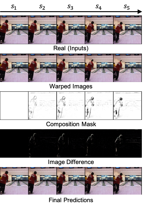
Figure 3: Visualization of three intermediate outputs (Warped Image, Image Difference, Composition Mask) during reconstructing images for video interpolation.

Image Difference $(\mathbf{D}_{s_{i}})$. Although using optical flow helps to capture video dynamics, the quality of the warped image often degrades when it comes to generating completely new pixels or facing a large motion. This is because, when there are big movements in the video, the warping operation moves a cluster of pixels to a new position and leaves an empty cluster behind. This becomes even more problematic when we try to predict multiple frames in an autoregressive manner. To tackle this challenge, we employ the image difference $\mathbf{D}_{s_{i}}\in\mathbb{R}^{m\times n\times c}$ at each $s_{i}$, which predicts the pixel-wise difference between the current frame and the previous frame, $\Delta\mathbf{X}_{s_{i}}$. Including $\mathbf{D}_{s_{i}}$ helps our model focus on areas where sudden movements take place.

Composition Mask $(\mathbf{M}_{s_{i}})$. The final output frame $\hat{\mathbf{X}}_{s_{i}}$ is generated by combining the warped image $\mathcal{W}(\mathbf{F}_{s_{i}},\hat{\mathbf{X}}_{s_{i-1}})$ and the image difference $\mathbf{D}_{s_{i}}$ using element-wise convex combination weighted by the composition mask $\mathbf{M}_{s_{i}}\in\mathbb{R}^{m\times n}$. While the other outputs of the Conv-Decoder $G$ (e.g., $\mathbf{F}_{s_{i}},\mathbf{D}_{s_{i}}$) have values in $[-\infty,\infty]$, $\mathbf{M}_{s_{i}}$ is forced to values in $[0,1]$ by a sigmoid activation, in order to perform its role as the convex combination weight. Figure 3 depicts the role played by $\mathbf{F}_{s_{i}},\mathbf{D}_{s_{i}}$, and $\mathbf{M}_{s_{i}}$ when generating a video. As seen in the warped images of Figure 3, the moving portion (i.e., head) is gradually faded away as the image warping is repeatedly applied. The image difference predicts the pixels, which can possibly have disappeared around large movements. Through combining these two outputs, we can obtain the improved results as seen in the last row of Figure 3.

Datasets	Model	Video Interpolation			Video Extrapolation
		SSIM↑	LPIPS↓	PSNR↑	SSIM↑	LPIPS↓	PSNR↑
KTH Action	Latent ODE	0.730	0.481	20.99	0.730	0.495	20.61
	ODE2VAE	0.752	0.456	23.28	0.755	0.430	23.19
	ODE-FC	0.749	0.444	22.96	0.750	0.442	23.00
	ODE-Conv	0.769	0.416	25.12	0.768	0.429	24.31
	Vid-ODE	0.911	0.048	31.77	0.878	0.080	28.19
Moving GIF	Latent ODE	0.700	0.483	15.69	0.675	0.513	14.41
	ODE2VAE	0.715	0.456	16.49	0.704	0.471	15.91
	ODE-FC	0.717	0.446	16.55	0.704	0.452	15.86
	ODE-Conv	0.745	0.380	17.88	0.713	0.429	16.23
	Vid-ODE	0.815	0.115	18.44	0.778	0.156	16.68
Penn Action	Latent ODE	0.377	0.762	15.63	0.374	0.775	15.32
	ODE2VAE	0.433	0.687	17.06	0.423	0.701	16.90
	ODE-FC	0.447	0.643	17.40	0.342	0.753	15.00
	ODE-Conv	0.550	0.538	19.25	0.557	0.514	19.23
	Vid-ODE	0.920	0.033	26.73	0.880	0.045	23.81

Table 1: Comparison with neural-ODE-based models

3.3 Objective Functions

Adversarial Loss We adopt two discriminators, one at the image level and the other at the video sequence level, to improve the output quality both in spatial appearance and temporal dynamics. The image discriminator $D_{\text{img}}$ distinguishes the real image $\mathbf{X}_{s_{i}}$ from the generated image $\hat{\mathbf{X}}_{s_{i}}$ for each target timestep $s_{i}$. The sequence discriminator $D_{\text{seq}}$ distinguishes a real sequence $\mathcal{X}_{\mathcal{S}}$ from the generated sequence $\hat{\mathcal{X}}_{\mathcal{S}}$ for all timesteps in $\mathcal{S}$. Specifically, we adopt LS-GAN (Mao et al. 2017) to model $D_{\text{img}}$ and $D_{\text{seq}}$ as

$$\min_{\text{Vid-ODE}}\max_{D_{\text{img}}}\mathcal{L}^{\text{img}}_{\text{adv}}=\mathbb{E}_{\mathbf{X}_{s_{i}}\sim p(\mathcal{X}_{\mathcal{S}})}\left[\left(D_{\text{img}}\left(\mathbf{X}_{s_{i}}\right)-1\right)^{2}\right]$$ (3)

$$\hskip 56.9055pt+\mathbb{E}_{\mathcal{X}_{\mathcal{T}}\sim p(\mathcal{X}_{\mathcal{T}})}\left[\left(D_{\text{img}}({\text{Vid-ODE}}(\hat{\mathbf{X}}_{s_{i}}|\mathcal{X}_{\mathcal{T}}))\right)^{2}\right]$$

$$\min_{\text{Vid-ODE}}\max_{D_{\text{seq}}}\mathcal{L}^{\text{seq}}_{\text{adv}}=\mathbb{E}_{\mathcal{X}_{t_{i}:s_{i}}\sim p(\mathcal{X}_{\mathcal{T;S}})}\left[\left(D_{\text{seq}}(\mathcal{X}_{t_{i}:s_{i}})-1\right)^{2}\right]$$ (4)

$$+\mathbb{E}_{\mathcal{X}_{t_{i}:s_{i-1}}\sim p(\mathcal{X}_{\mathcal{T;S}})}\left[\left(D_{\text{seq}}\big{(}\mathcal{X}_{t_{i}:s_{i-1}};{\text{Vid-ODE}}(\hat{\mathbf{X}}_{s_{i}}|\mathcal{X}_{\mathcal{T}})\big{)}\right)^{2}\right],$$

where $\mathcal{T;S}$ is union of the timesteps $\mathcal{T}$ and $\mathcal{S}$, and $\mathcal{X}_{t_{i}:s_{i}}$ is a sequence of frames from $t_{i}$ to $T$, concatenated with frames from $s_{1}$ to $s_{i}$, for some $i=1,\ldots,K$.

Reconstruction Loss. $\mathcal{L}_{\text{recon}}$ computes the pixel-level $L_{1}$ distance between the predicted video frame $\hat{\mathbf{X}}_{s_{i}}$ and the ground-truth frame $\mathbf{X}_{s_{i}}$. Formally,

$$\mathcal{L}_{\text{recon}}=\mathbb{E}_{\mathbf{X}_{s_{i}}\sim\mathcal{X}_{\mathcal{S}}}\left[\|\hat{\mathbf{X}}_{s_{i}}-\mathbf{X}_{s_{i}}\|_{1}\right].$$ (5)

Difference Loss $\mathcal{L}_{\text{diff}}$ helps the model learn the image difference $\mathbf{D}_{s_{i}}$ as the pixel-wise difference between consecutive video frames. Formally,

$$\mathcal{L}_{\text{diff}}=\mathbb{E}_{\Delta\mathbf{X}_{s_{i}}\sim\Delta\mathcal{X}_{\mathcal{S}}}\left[\|\mathbf{D}_{s_{i}}-\Delta\mathbf{X}_{s_{i}}\|_{1}\right],$$ (6)

where $\Delta\mathbf{X}_{s_{i}}$ denotes the image difference between two consecutive frames, i.e., $\mathbf{X}_{s_{i}}-\mathbf{X}_{s_{i-1}}$.

Overall Objective Vid-ODE is trained end-to-end using the following objective function:

$$\mathcal{L}=\mathcal{L}_{\text{recon}}+\lambda_{\text{diff}}\mathcal{L}_{\text{diff}}+\lambda_{\text{img}}\mathcal{L}^{\text{img}}_{\text{adv}}+\lambda_{\text{seq}}\mathcal{L}^{\text{seq}}_{\text{adv}},$$ (7)

where we use $\lambda_{\text{diff}}$, $\lambda_{\text{img}}$, and $\lambda_{\text{seq}}$ for hyper-parameters controlling relative importance between different losses.

4 Experiments

4.1 Experimental Setup

We evaluate our model on two tasks: video interpolation and video extrapolation. In video interpolation, a sequence of five input frames are given, and the model is trained to reconstruct the input frames during the training phase. At inference, it predicts the four intermediate frames between the input time steps. In video extrapolation, given a sequence of five input frames, the model is trained to output the next five future frames, which are available in training data. At inference, it predicts the next five frames. We conclude this section with the analysis of the role of each component of Vid-ODE, including an ablation study.

Evaluation Metrics. We evaluate our model using two metrics widely-used in video interpolation and video extrapolation, including Structural Similarity (SSIM) (Wang et al. 2004), Peak Signal-to-Noise Ratio (PSNR). In addition, we use Learned Perceptual Image Patch Similarity (LPIPS) (Zhang et al. 2018) to measure a semantic distance between a pair of the real and generated frames. Higher is better for SSIM and PSNR, lower is better for LPIPS.

Datasets. For our evaluation, we employ and preprocess the four real-world datasets and the one synthetic dataset as follows:

KTH Action (Schuldt, Laptev, and Caputo 2004) consists of 399 videos of 25 subjects performing six different types of actions (walking, jogging, running, boxing, hand waving, and hand clapping). We use 255 videos of 16 (out of 25) subjects for training and the rest for testing. The spatial resolution of this dataset is originally $160\times 120$, but we center-crop and resize it to $128\times 128$ for both training and testing.

Moving GIF (Siarohin et al. 2019) consists of 1,000 videos of animated animal characters, such as tiger, dog, and horse, running or walking in a white background. We use 900 for training and 100 for testing. The spatial resolution of the original dataset is $256\times 256$, and each frame is resized to $128\times 128$ pixels. Compared to other datasets, Moving GIF contains relatively larger movement, especially in the legs of cartoon characters.

Penn Action (Zhang, Zhu, and Derpanis 2013) consists of videos of humans playing sports. The dataset contains 2,326 videos in total, involving 15 different sports actions, including baseball swing, bench press, and bowling. The resolution of the frames is within the size of $640\times 480$. For training and testing, we center-crop each frame and then resize it to $128\times 128$ pixels. We use 1,258 videos for training and 1,068 for testing.

CAM5 (Kim et al. 2019) is a hurricane video dataset, where we evaluate our model on video extrapolation for irregular-sampled input videos. This dataset contains the frames of the global atmospheric states for every 3 hours with around $0.25^{\circ}$ resolution, using the annotated hurricane records from 1996 to 2015. We use zonal wind (U850), meridional wind (V850), and sea-level pressure (PSL) out of multiple physical variables available in each frame. We take only those time periods during which hurricane actually occurs, resulting in 319 videos. We use 280 out of these for training and 39 for testing. To fit large-scale global climate videos into GPU memory, we split the global map into several non-overlapping basins of $60^{\circ}\times 160^{\circ}$ sub-images.

Bouncing Ball contains three balls moving in different directions with a resolution of $32\times 32$, where we evaluate our model for video extrapolation when non-linear motions occur as videos proceed. We use 1,000 videos for training and 50 videos for testing.

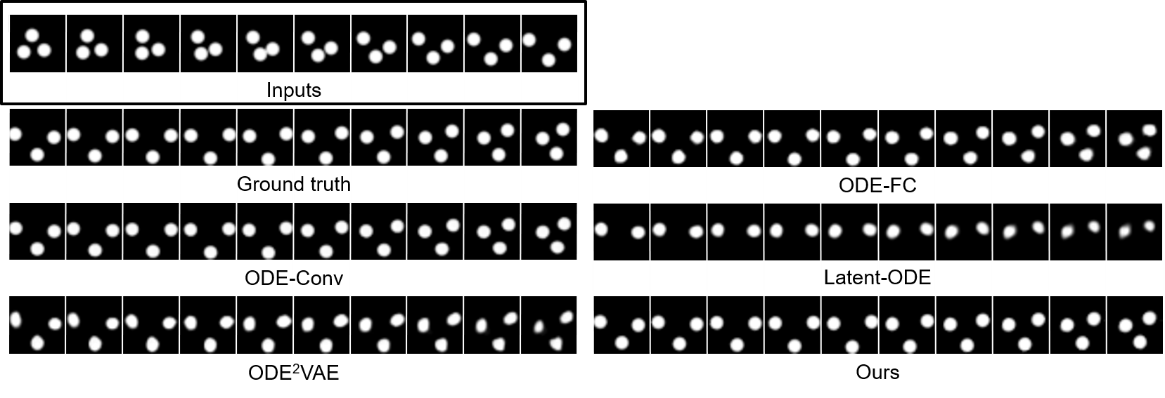
Figure 4: Video extrapolation results of Vid-ODE and baseline models from the Bouncing ball dataset.

Datasets	Model	SSIM↑	LPIPS↓	PSNR↑
KTH Action	ConvGRU	0.764	0.379	21.52
	PredNet	0.825	0.242	22.15
	DVF	0.837	0.129	26.05
	RCG	0.820	0.187	21.92
	Vid-ODE	0.878	0.080	28.19
Moving GIF	ConvGRU	0.467	0.532	11.49
	PredNet	0.649	0.232	14.64
	DVF	0.777	0.215	16.39
	RCG	0.593	0.491	11.17
	Vid-ODE	0.778	0.156	16.68
Penn Action	ConvGRU	0.625	0.262	18.48
	PredNet	0.840	0.073	19.01
	DVF	0.790	0.102	21.90
	RCG	0.809	0.098	20.13
	Vid-ODE	0.880	0.045	23.81

Table 2: Video extrapolation results

Implementation Details. We employ Adamax (Kingma and Ba 2014), a widely-used optimization method to iteratively train the ODE-based model. We train Vid-ODE for 500 epochs with a batch size of 8. The learning rate is set initially as 0.001, then exponentially decaying at a rate of 0.99 per epoch. In addition, we find that Vid-ODE shows a slight performance improvement when the input frames are in reverse order. A horizontal flip and a random rotation in the range of -10 to 10 degrees are used for data augmentation. For the implementations of existing baselines, we follow the hyperparameters given in the original papers and conduct the experiments with the same number of epochs, the batch size, and data augmentation as our model. For hyperparameters of Vid-ODE, we use $\lambda_{\text{diff}}=1.0$, $\lambda_{\text{img}}=0.003$, and $\lambda_{\text{seq}}=0.003$. As for training ODEs, Vid-ODE required only 7 hours for training on the KTH Action dataset using a single NVIDIA Titan RTX (using 6.5GB VRAM).

Datasets	Model	SSIM↑	LPIPS↓	PSNR↑
KTH Action	DVF	0.954	0.037	36.28
	UVI	0.934	0.055	29.97
	Vid-ODE	0.911	0.048	31.77
Moving GIF	DVF	0.850	0.130	19.41
	UVI	0.700	0.163	17.13
	Vid-ODE	0.815	0.115	18.44
Penn Action	DVF	0.955	0.024	30.11
	UVI	0.904	0.042	25.21
	Vid-ODE	0.920	0.033	26.73

Table 3: Video interpolation results. We compare Vid-ODE (unsupervised) with DVF (supervised) and UVI (unupservised).

4.2 Comparison with Neural-ODE-based Models

Quantitative Comparison. We compare Vid-ODE against existing neural-ODE-based models such as ODE²VAE (Yildiz, Heinonen, and Lahdesmaki 2019) and latent ODE (Rubanova, Chen, and Duvenaud 2019). In addition, to verify the effectiveness of ODE-ConvGRU described in Section 3.1, we design the variants of neural ODEs (e.g., ODE-FC, ODE-Conv) by removing ODE-ConvGRU; thus, both take the channel-wise concatenated frames as an input for the Conv-Encoder $E$. We call the variants depending on the types of the derivative function $f_{\phi}$: fully-connected layers (ODE-FC) and convolutional layers (ODE-Conv).

Table 1 shows that Vid-ODE significantly outperforms all other baselines both in interpolation and extrapolation tasks. This improvement can be attributed to the ODE-ConvGRU and the linear composition, which helps Vid-ODE effectively maintain spatio-temporal information while preserving the sharpness of the outputs. This is also supported by an observation that ODE-Conv outperforms ODE-FC, achieving higher scores by simply using convolutional layers to estimate the derivatives of hidden states where spatial information resides. We find that the VAE architecture of ODE²VAE and Latent ODE makes the training unstable, as the KL divergence loss of high dimensional representations does not converge well. Due to this, these models often fail to generate realistic images, resulting in suboptimal performance. Qualitative results are reported in the supplementary material.

Figure 5: Video extrapolation results of Vid-ODE and baseline models from KTH-Action.

Non-linear Motion. We validate the effectiveness of Vid-ODE in handling a non-linear motion using bouncing ball dataset. Given a sequence of 10 input frames, the model is trained to predict the next 10 future frames. The motion of a ball often involves abrupt changes in its moving direction when it hits the wall, which can be viewed as a clear example of a non-linear motion. As seen in the first half of the second row of Fig 4, we can observe the non-linear, bouncing movement of a ball at the bottommost. Although such dynamics are non-linear, as shown in Fig 4, our model successfully predicts the reflection. Not surprisingly, most baselines work well, yet Vid-ODE still outperforms the baselines, demonstrating its superiority even on a low-dimensional dataset.

4.3 Comparison with Task-specific Models

We compare the performance of Vid-ODE against various state-of-the-art video interpolation (Liu et al. 2017; Reda et al. 2019) and extrapolation models (Ballas et al. 2015; Lotter, Kreiman, and Cox 2016; Kwon and Park 2019; Liu et al. 2017).

Video Extrapolation. As baselines, we adopt PredNet (Lotter, Kreiman, and Cox 2016), Deep Voxel Flow(DVF) (Liu et al. 2017), Retrospective Cycle GAN(RCG) (Kwon and Park 2019). As shown in Table 2, Vid-ODE significantly outperforms all other baseline models in all metrics. It is noteworthy that the performance gap is wider for Moving GIF, which contains more dynamic object movements (compared to rather slow movements in KTH-Action and Penn-Action), indicating Vid-ODE’s superior ability to learn complex dynamics. Furthermore, qualitative comparison shown in Figure 5 demonstrates that our model successfully learns the underlying dynamics of the object, and generates more realistic frames compared to baselines. In summary, Vid-ODE not only generates superior video frames compared to various state-of-the-art video extrapolation models, but also has the unique ability to generate frames at arbitrary timesteps.

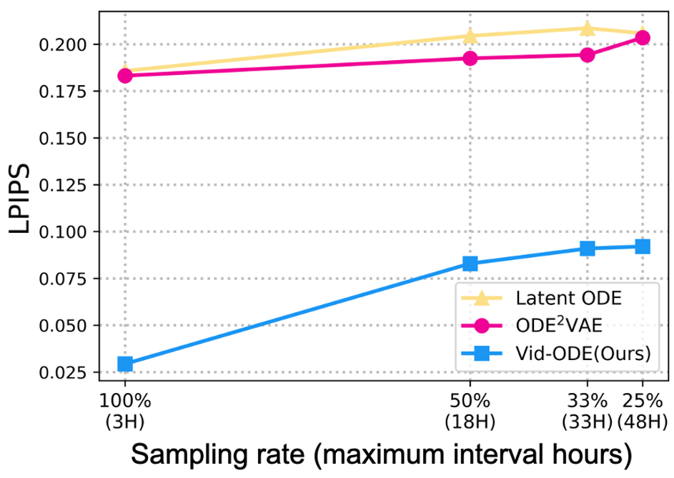
Figure 6: Change of LPIPS at different sampling rates. Vid-ODE outperforms the baselines at all sampling rates and shows relatively small declines in performance as inputs are sparsely drawn.

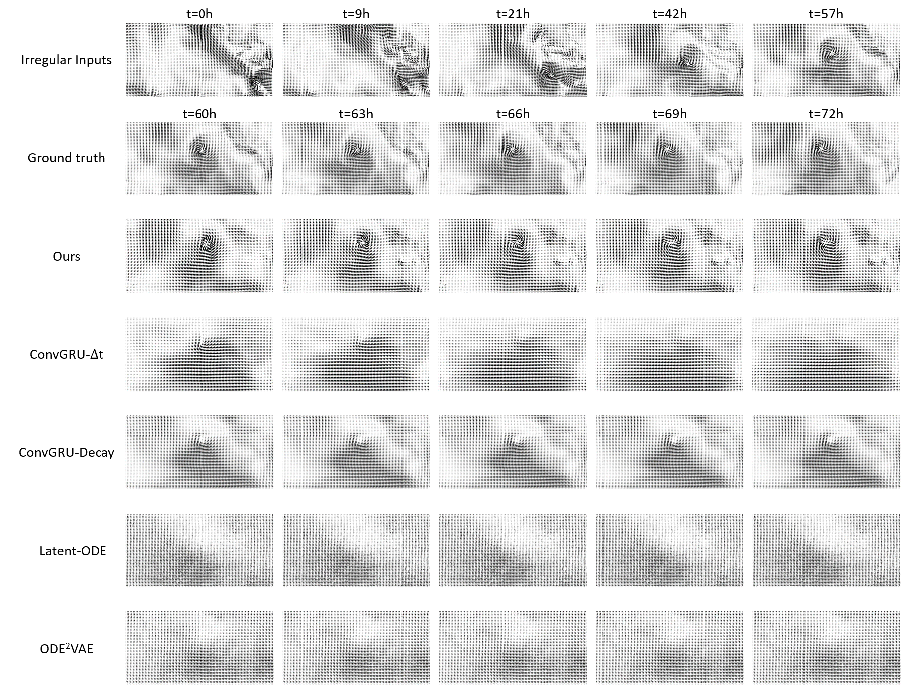
Figure 7: Qualitative comparisons with the baselines on the CAM5 hurricane dataset. For input, we sample 5 frames with different intervals (first row; i.e., 0, 9, 21, 42, and 57 hours). Given the irregularly sampled frames, every model including Vid-ODE predicts the frames at regular timesteps (i.e., 60, 63, 66, 69, and 72 hours). For visualization, we use zonal wind (U850) and meridional wind (V850) together to represent the vector at each pixel. Our model outperforms the baselines, successfully synthesizing the shape and the trajectory of the hurricane.

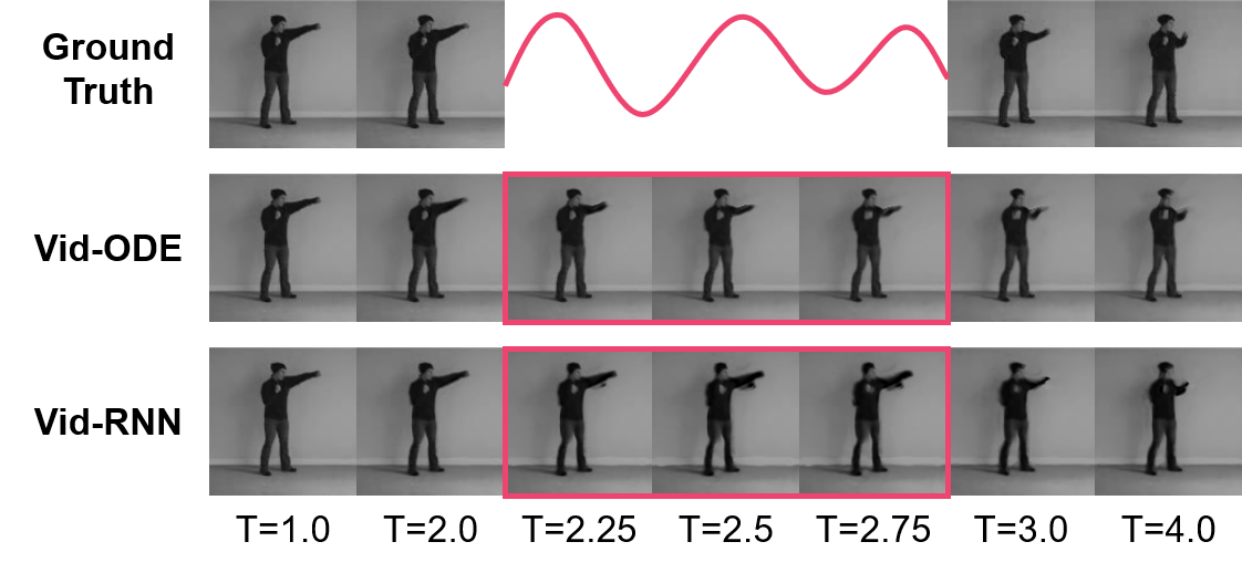
Figure 8: Comparison between Vid-ODE and Vid-RNN, which has the same architecture as Vid-ODE except all ODE components are replaced with RNNs, interpolating non-existing in-between frames at arbitrary timesteps.

Video Interpolation. We compare Vid-ODE with Unsupervised Video Interpolation (UVI) (Reda et al. 2019), which is trained to interpolate in-between frames in an unsupervised manner. We additionally compare with a supervised interpolation method, DVF (Liu et al. 2017), to measure the headroom for potential further improvement. As shown in Table 3, Vid-ODE outperforms UVI in all cases (especially in Moving GIF), except for SSIM in KTH-Action. As expected, we see some gap between Vid-ODE and the supervised approach (DVF).

Methods	Video Interpolation			Video Extrapolation
	SSIM↑	LPIPS↓	PSNR↑	SSIM↑	LPIPS↓	PSNR↑
($\mathtt{A}$) ODE-Conv	0.769	0.416	25.12	0.768	0.429	24.31
($\mathtt{B}$) Vanilla Vid-ODE	0.864	0.247	27.81	0.853	0.262	26.49
($\mathtt{C}$) + Adversarial learning	0.866	0.226	28.60	0.856	0.245	27.69
($\mathtt{D}$) + Optical flow warping	0.912	0.052	31.60	0.862	0.085	28.30
($\mathtt{E}$) + Mask composition	0.911	0.048	31.77	0.878	0.080	28.19

Table 4: Performance improvement by adding each component to the Vid-ODE suggesting the applicability of each component to improve performance of tasks.

Datasets	Model	LPIPS↓	MSE↓
CAM5	ConvGRU-$\Delta$t	0.270	2.439
	ConvGRU-Decay	0.160	0.583
	Latent ODE	0.206	0.554
	ODE2VAE	0.203	0.551
	Vid-ODE	0.092	0.515

Table 5: Extrapolation results for irregularly-sampled input video from the CAM5 hurricane dataset. MSE ($\times$ 10^-3)

Irregular Video Prediction. One of the distinguishing aspects of Vid-ODE is its ability to handle videos of an arbitrary sampling rate. We use CAM5 to test Vid-ODE’s ability to cope with irregularly sampled input, where we force the model to extrapolate at a higher rate (i.e. every three hours) than the input’s sampling rate. We randomly sample 5 input frames from each hurricane video where the interval can be as large as 48 hours. For baselines, we use Latent ODE, ODE²VAE (Yildiz, Heinonen, and Lahdesmaki 2019), ConvGRU-$\Delta_{t}$, and ConvGRU-Decay where the last two were implemented by replacing the RNN cell of RNN-$\Delta_{t}$ and RNN-Decay (Che et al. 2018) to ConvGRU (Ballas et al. 2015). Table 5 shows that Vid-ODE outperforms baselines in both LPIPS and MSE, demonstrating the Vid-ODE’s ability to process irregularly sampled video frames. Furthermore, visual comparison shown in Figure 7 demonstrates the capacity of Vid-ODE to handle spatial-temporal dynamics from irregularly sampled inputs. Lastly, we measure MSE and LPIPS on CAM5 dataset while changing the input’s sampling rate to evaluate the effect of irregularity. As shown in Figure 6, all models perform worse as sampling rate decreases, demonstrating the difficulty of handling the sparsely sampled inputs. Still, Vid-ODE outperforms the baselines at the irregularly sampled inputs as well as regularly sampled inputs ($i.e.,$ 100$\%$ sampling rate), which verify its superior capability to cope with irregular inputs.

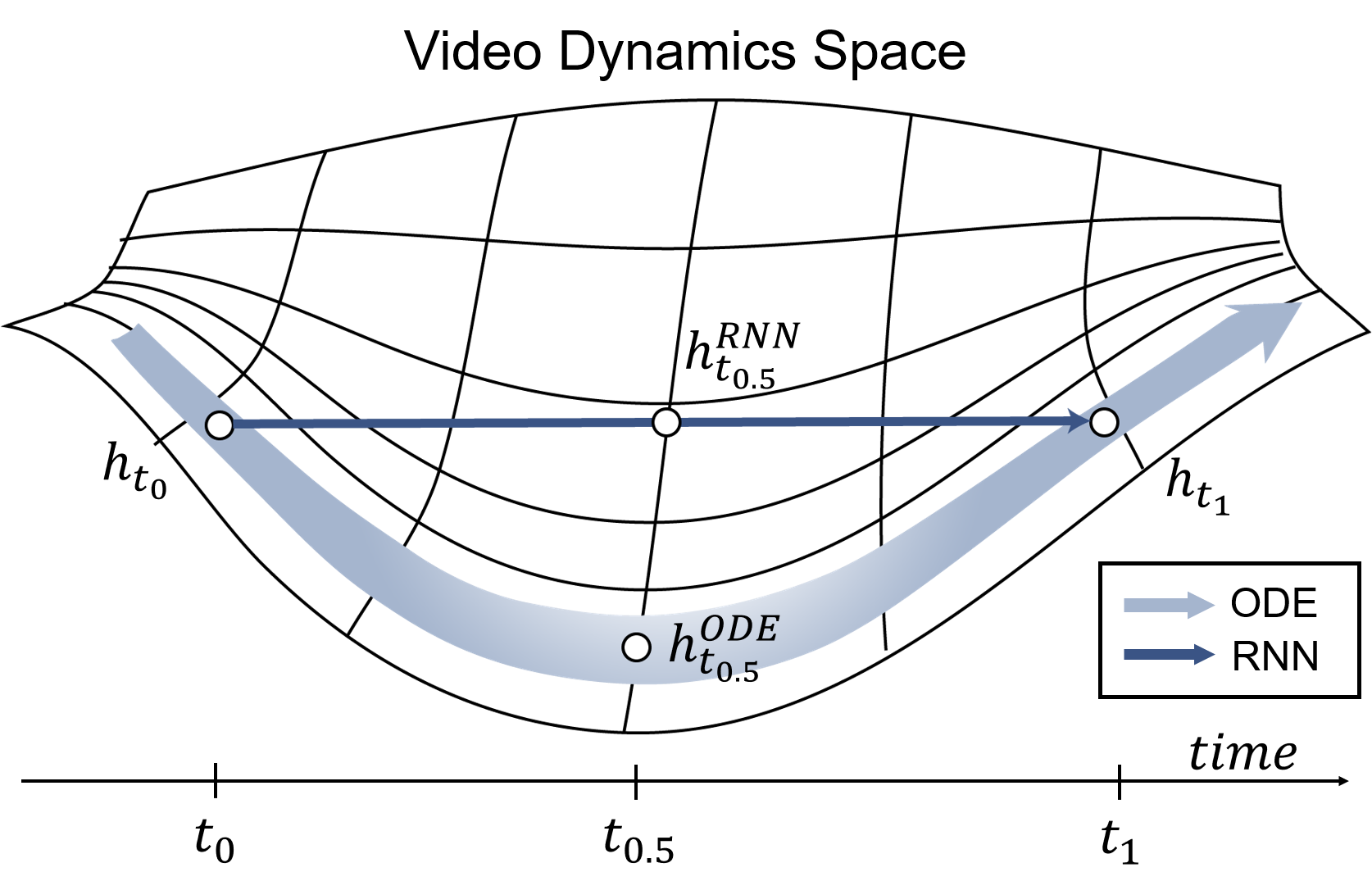
Figure 9: In the video dynamics space, RNN is limited to learn the representations only at observed timesteps ($t_{0},t_{1}$). On the other hand, Vid-ODE is encouraged to learn the entire geometry, enabling it to generate video frames at unseen timesteps ($t_{0.5}$).

4.4 Analysis of Individual Components

Need for Learning the Continuous Video Dynamics. To emphasize the need for learning the continuous video dynamics using the ODE, we compare Vid-ODE to Vid-RNN, which replaces ODE components in both the encoder and decoder of Vid-ODE with ConvGRU while retaining all other components such as linear composition. Using Vid-RNN, we can obtain video representations at arbitrary timesteps by interpolating its decoder (ConvGRU) hidden states from two adjacent regular timesteps. If Vid-RNN could generate video frames at unseen timesteps as well as Vid-ODE, then an ODE-based video generation would be unnecessary. However, Figure 8 shows that is not the case. While Vid-ODE is successfully inferring video frames at unseen timesteps ($t=2.25,t=2.5,t=2.75$) thanks to learning the underlying video dynamics, Vid-RNN generates unrealistic video frames due to simply blending two adjacent latent representations. The intuition behind such behavior is described in Figure 9, where the advantage of the ODE-based approach is evident when handling continuous time.

Ablation Study. Table 4 depicts the effectiveness of each component of the Vid-ODE. Starting with a simple baseline ODE-Conv $\mathtt{(A)}$, we first compare vanilla Vid-ODE $\mathtt{(B)}$ equipped with the proposed ODE-ConvGRU. We see a significant boost in performance, meaning that the ODE-ConvGRU cell better captures spatio-temporal dynamics in the video and is able to generate high-quality frames. As depicted by $\mathtt{(C)}$ in Table 4, adding the adversarial loss to $\mathtt{(B)}$ improves performance, especially in LPIPS, suggesting that the image and sequence discriminators help the model generate realistic images. From $\mathtt{(C)}$ to $\mathtt{(D)}$, we add the optical flow warping (Eq. (2)), which significantly enhances the performance by effectively learning the video dynamics. As the last component, we add the linear composition $\Psi$ ($\mathtt{E}$). The performance boost from $\mathtt{(D)}$ to $\mathtt{(E)}$ might seem marginal. Comparing the warped image with the final product in Figure 3, however, demonstrates that using the image difference to fill in the disappeared pixels in the warped image indeed enhances the visual quality of the output.

5 Conclusions

In this paper, we propose Vid-ODE which enjoys the continuous nature of neural ODEs to generate video frames at any given timesteps. Combining the ODE-ConvGRU with the linear composition of optical flow and image difference, Vid-ODE successfully demonstrates its ability to generate high-quality video frames in the continuous-time domain using four real-world video datasets for both video interpolation and video extrapolation. Despite its success in continuous-time video generation, Vid-ODE tends to yield degraded outcomes as the number of predictions increases because of its autoregressive nature. In future work, we plan to study how to adopt a flexible structure to address this issue.

Ethical Impact

Our proposed Vid-ODE model learns the continuous flow of videos from a sequence of frames from potentially irregular training data and is capable of synthesizing new frames at any given timesteps. Our framework is applicable to the broad scope of spatio-temporal data without limiting to multi-media data. For example, as discussed in the main sections, this can be especially useful for scientific data where the assumption of regularly sampled time step does not always hold. Specifically, the application of the proposed model to climate data, where the measurement is costly and sparse while it is sometimes beneficial to forecast at the denser rate, is critical. This can potentially bring a significant impact on weather forecasting with improved estimation quality as well as with less cost compared to traditional scientific models. For instance, in disaster prevention plans for extreme climate events, the decision-makers often rely on simulation or observation data with sparse timesteps, which is only available out there. This limits the capability to forecast in more frequent timesteps and thus prevent solid decisions based on accurate disaster scenarios. Our Vid-ODE takes a significant step towards a fully data-driven approach to forecasting extreme climate events by addressing this issue.

Supplementary Material

A. Implementation Details

We employ Adamax [15], a widely-used optimization method to iteratively train the ODE-based model. We train Vid-ODE for 500 epochs with a batch size of 8. The learning rate is set initially as 0.001, then exponentially decaying at a rate of 0.99 per epoch. In addition, we find that Vid-ODE shows a slight performance improvement when the input frames are in a reverse order. A horizontal flip and a random rotation in the range of -10 to 10 degrees are used for data augmentation. For the implementations of existing baselines, we follow the hyperparameters given in the original papers and conduct the experiments with the same number of epochs, the batch size and data augmentation as our model. For hyperparameters of Vid-ODE, we use $\lambda_{\text{diff}}=1.0$, $\lambda_{\text{img}}=0.003$, and $\lambda_{\text{seq}}=0.003$. As for training ODEs, Vid-ODE required only 7 hours for training on KTH Action dataset using a single NVIDIA Titan RTX (using 6.5GB VRAM).

5.1 Adversarial Loss for Interpolation

For video interpolation, we make the generated sequence $\hat{\mathcal{X}}_{\mathcal{S}}$ for all timesteps by alternatively substituting a real frame in $\mathcal{X}_{\mathcal{T}}$ with a fake frame $\hat{\mathbf{X}}_{s_{i}}$. Formally, $\mathcal{L}^{\text{img}}_{\text{adv}}$ and $\mathcal{L}^{\text{seq}}_{\text{adv}}$ are formulated as

$$\min_{\text{Vid-ODE}}\max_{D_{\text{img}}}\mathcal{L}^{\text{img}}_{\text{adv}}=\mathbb{E}_{\mathbf{X}_{s_{i}}\sim p(\mathcal{X}_{\mathcal{S}})}\left[\left(D_{\text{img}}\left(\mathbf{X}_{s_{i}}\right)-1\right)^{2}\right]$$

$$\hskip 62.59596pt+\mathbb{E}_{\mathcal{X}_{\mathcal{T}}\sim p(\mathcal{X}_{\mathcal{T}})}\left[\left(D_{\text{img}}({\text{Vid-ODE}}(\hat{\mathbf{X}}_{s_{i}}|\mathcal{X}_{\mathcal{T}}))\right)^{2}\right]$$

$$\min_{\text{Vid-ODE}}\max_{D_{\text{seq}}}\mathcal{L}^{\text{seq}}_{\text{adv}}=\mathbb{E}_{\mathcal{X}_{\mathcal{T}}\sim p(\mathcal{X}_{\mathcal{T}})}\left[\left(D_{\text{seq}}(\mathcal{X}_{\mathcal{T}})-1\right)^{2}\right]$$

$$+\mathbb{E}_{\mathcal{X}_{\mathcal{T}}\sim p(\mathcal{X}_{\mathcal{T}})}\left[\left(D_{\text{seq}}\big{(}\mathcal{X}_{t_{0}:t_{i-1}};{\text{Vid-ODE}}(\hat{\mathbf{X}}_{s_{i}}|\mathcal{X}_{\mathcal{T}});\mathcal{X}_{t_{i+1}:t_{L}}\big{)}\right)^{2}\right],$$ (8)

where $\mathcal{X}_{t_{0}:t_{i-1}};{\text{Vid-ODE}}(\hat{\mathbf{X}}_{s_{i}}|\mathcal{X}_{\mathcal{T}});\mathcal{X}_{t_{i+1}:t_{L}}$ denotes a modified input sequence in which an intermediate frame $\mathbf{X}_{t_{i}}$ is replaced by the predicted frame $\hat{\mathbf{X}}_{s_{i}}$ (Recall that $s_{i}=t_{i}$ for interpolation). Note that $\mathcal{X}_{t_{0}:t_{0}}=\mathcal{X}_{t_{L}:t_{L}}=\emptyset$, meaning that concatenation only occurs at backward or forward when $i=1$ and $i=L-1$, respectively.

5.2 Model Architecture

Vid-ODE architectures are shown in Tables 6-8. The notations used are as follows; N: the number of the output channels, K: the kernel size, S: the stride size, P: the padding size, BN: batch normalization, Up: bilinear upsampling $\times 2$.

B. Architectures of Vid-ODE and Vid-RNN

We compare Vid-ODE and Vid-RNN to demonstrate the superior capability of the ODE component to learn continuous video dynamics. Vid-RNN is built by replacing ODE components in Vid-ODE with ConvGRU while retaining all other components such as adversarial losses and the linear composition. Figure 10 shows the the architectures of Vid-ODE and Vid-RNN. To clearly illustrate the main components of the architectures, we omit the detailed components of decoding phase such as optical flow and linear composition.

Figure 10: The architectures of Vid-ODE and Vid-RNN for continuous video interpolation. The main difference between Vid-ODE and Vid-RNN lies in how to obtain the representations at unseen timesteps. In order to generate the frames at unseen timesteps, we interpolate the hidden states of Vid-RNN decoder from two observed timesteps. The unseen frames are not used during training of Vid-RNN to make the same settings as Vid-ODE.

C. Additional Experiments

This section presents additional experiments as follows:

• Quantitative comparison results against the stochastic video prediction baselines.

• Quantitative comparison results given irregularly sampled inputs at different sampling rates.

• Qualitative comparison results with the video interpolation and extrapolation baselines.

• Continuous video generation results in varying time intervals based on 5-FPS input videos.

• High-resolution (e.g., $256\times 256$) video interpolation and extrapolation results on Penn Action dataset.

Additional Comparison with Baselines. In order to further evaluate our method, we additionally compare Vid-ODE with SVG-FP, SVG-LP [6], SAVP [17], and SRVP [9] for extrapolation. We used the official codes provided by the authors and followed the hyperparameters as presented in the official codes. Table 9 shows Vid-ODE consistently outperforms these existing approaches (except for one metric).

Video Interpolation. Figures 11–13 illustrate video interpolation, where we generate 4 frames in-between the given 5 input frames. The locations with highly dynamic movements are marked with rectangles (red for inputs and ground truth, green for Vid-ODE results).

Video Extrapolation. Figures 14–16 illustrate video extrapolation on KTH, Moving GIF, and Penn Action datasets, where we compare the 5 predicted future frames given 5 previous input frames. We mark the areas with highly dynamic movements in the same manner as video interpolation.

Continuous Video Interpolation. In Figures 17–18, given 5 frames as an input, we visualize videos generated in various FPS (e.g., 8, 11, 14, 17, and 20 FPS) between the first frame and the last frame.

Continuous Video Extrapolation. In Figures 19–20, we generate future frames in various FPS (e.g., 8, 11, 14, 17, and 20 FPS) after the last input frame.

High-resolution video generation. As shown in Figure 21–22, we further demonstrate that Vid-ODE works well for higher resolution (256$\times$256) videos. Moving parts and their directions are marked with yellow arrows.

Part	Layer	Output Shape	Layer Information
Input Image	-	$(h,w,c)$	-
Conv-Encoder $E$	Downsample	$(h/2,w/2,32)$	Conv-(N32, K3$\times$3, S1, P1), BN, ReLU
	Downsample	$(h/2,w/2,64)$	Conv-(N32, K4$\times$4, S2, P1), BN, ReLU
	Downsample	$(h/4,w/4,128)$	Conv-(N32, K4$\times$4, S2, P1), BN, ReLU
ODE-ConvGRU	ConvGRU	$(h/4,w/4,128)$	Conv-(N128, K3$\times$3, S1, P1)
	ODE Func $f_{\theta}$	$(h/4,w/4,128)$	Conv-(N128, K3$\times$3, S1, P1), Tanh
	ODE Func $f_{\theta}$	$(h/4,w/4,128)$	Conv-(N128, K3$\times$3, S1, P1), Tanh
	ODE Func $f_{\theta}$	$(h/4,w/4,128)$	Conv-(N128, K3$\times$3, S1, P1), Tanh
	ODE Func $f_{\theta}$	$(h/4,w/4,128)$	Conv-(N128, K3$\times$3, S1, P1)

Table 6: Encoder architecture of our model.

Part	Layer	Output Shape	Layer Information
ODE Solver	ODE Func $f_{\phi}$	$(h/4,w/4,128)$	Conv-(N128, K3$\times$3, S1, P1), Tanh
	ODE Func $f_{\phi}$	$(h/4,w/4,128)$	Conv-(N128, K3$\times$3, S1, P1), Tanh
	ODE Func $f_{\phi}$	$(h/4,w/4,128)$	Conv-(N128, K3$\times$3, S1, P1), Tanh
	ODE Func $f_{\phi}$	$(h/4,w/4,128)$	Conv-(N128, K3$\times$3, S1, P1)
Conv-Decoder $G$	Upsample	$(h/2,w/2,128)$	Up, Conv-(N128, K3$\times$3, S1, P1), BN, ReLU
	Upsample	$(h,w,64)$	Up, Conv-(N64, K3$\times$3, S1, P1), BN, ReLU
	Upsample	$(h,w,c+3)$	Up, Conv-(N(c+3), K3$\times$3, S1, P1)

Table 7: Decoder architecture of our model.

Part	Layer	Output Shape	Layer Information
Input Image	-	$(h,w,c)$	-
Discriminator $D_{\text{img}}$	Downsample	$(h/2,w/2,64)$	Conv-(N64, K4$\times$4, S2, P1), LeakyReLU
	Downsample	$(h/4,w/4,128)$	Conv-(N128, K4$\times$4, S2, P1), LeakyReLU
	Downsample	$(h/8,w/8,256)$	Conv-(N256, K4$\times$4, S2, P1), LeakyReLU
	Downsample	$(h/8,w/8,512)$	Conv-(N512, K4$\times$4, S1, P2), LeakyReLU
	Downsample	$(h/8,w/8,64)$	Conv-(N64, K4$\times$4, S1, P2)
Input Sequence	-	$(h,w,c\times t)$	-
Discriminator $D_{\text{seq}}$	Downsample	$(h/2,w/2,64)$	Conv-(N64, K4$\times$4, S2, P1), LeakyReLU
	Downsample	$(h/4,w/4,128)$	Conv-(N128, K4$\times$4, S2, P1), LeakyReLU
	Downsample	$(h/8,w/8,256)$	Conv-(N256, K4$\times$4, S2, P1), LeakyReLU
	Downsample	$(h/8,w/8,512)$	Conv-(N512, K4$\times$4, S1, P2), LeakyReLU
	Downsample	$(h/8,w/8,64)$	Conv-(N64, K4$\times$4, S1, P2)

Table 8: Discriminator architecture of our model.

Model	KTH Action			Moving GIF			Penn Action
	SSIM↑	LPIPS↓	PSNR↑	SSIM↑	LPIPS↓	PSNR↑	SSIM↑	LPIPS↓	PSNR↑
SVG-FP	0.848	0.156	26.34	0.682	0.254	15.62	0.815	0.099	21.53
SVG-LP	0.843	0.157	22.24	0.710	0.233	15.95	0.814	0.117	21.36
SAVP	0.885	0.089	27.40	0.722	0.163	15.66	0.822	0.074	22.23
SRVP	0.831	0.113	27.79	0.667	0.263	16.23	0.877	0.056	22.10
Vid-ODE	0.878	0.080	28.19	0.778	0.156	16.68	0.880	0.045	23.81

Table 9: Additional video extrapolation comparisons. We report the baseline results by taking the average of three samples.

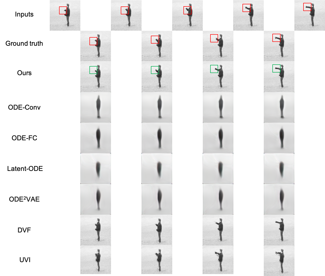
Figure 11: Qualitative comparisons with interpolation baselines on the KTH Action dataset.

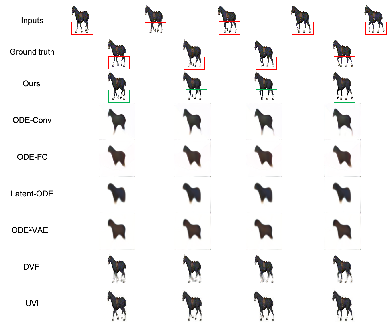
Figure 12: Qualitative comparisons with interpolation baselines on the Moving GIF dataset.

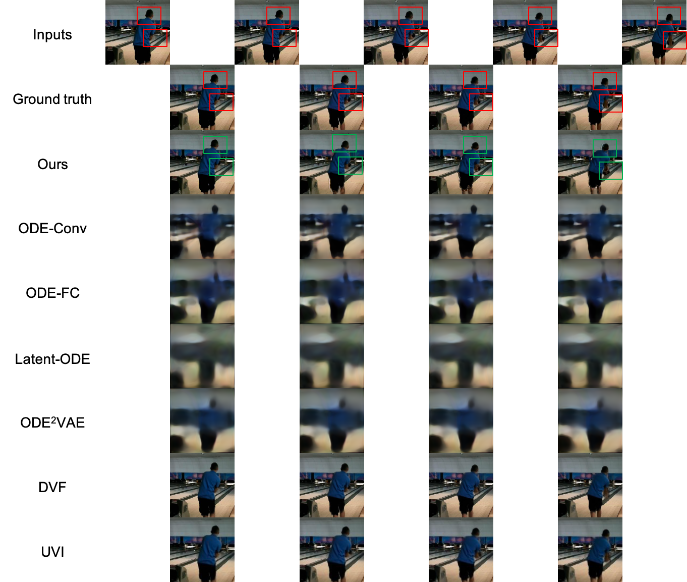
Figure 13: Qualitative comparisons with interpolation baselines on the Penn Action dataset.

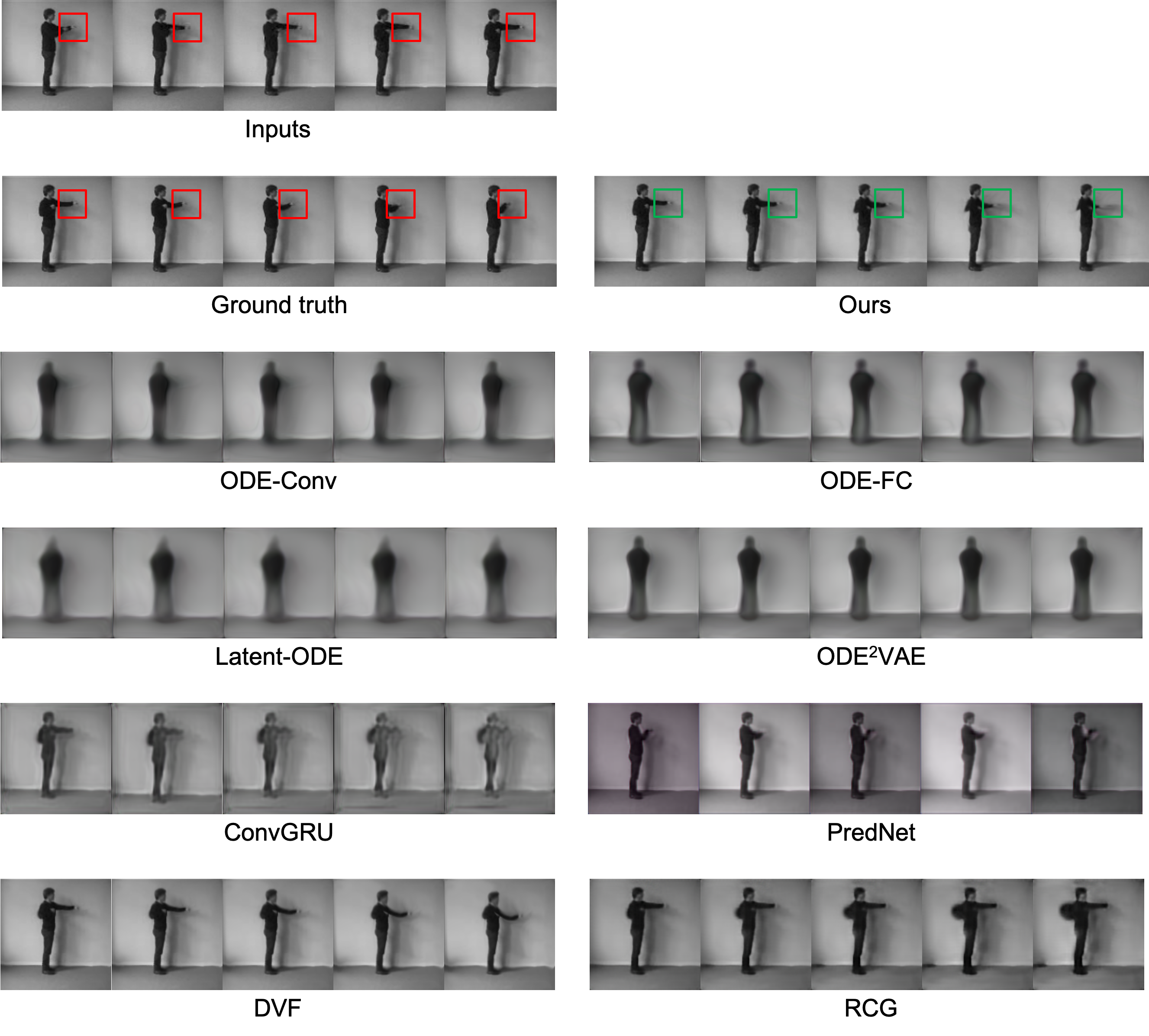
Figure 14: Qualitative comparisons with extrapolation baselines on the KTH Action dataset.

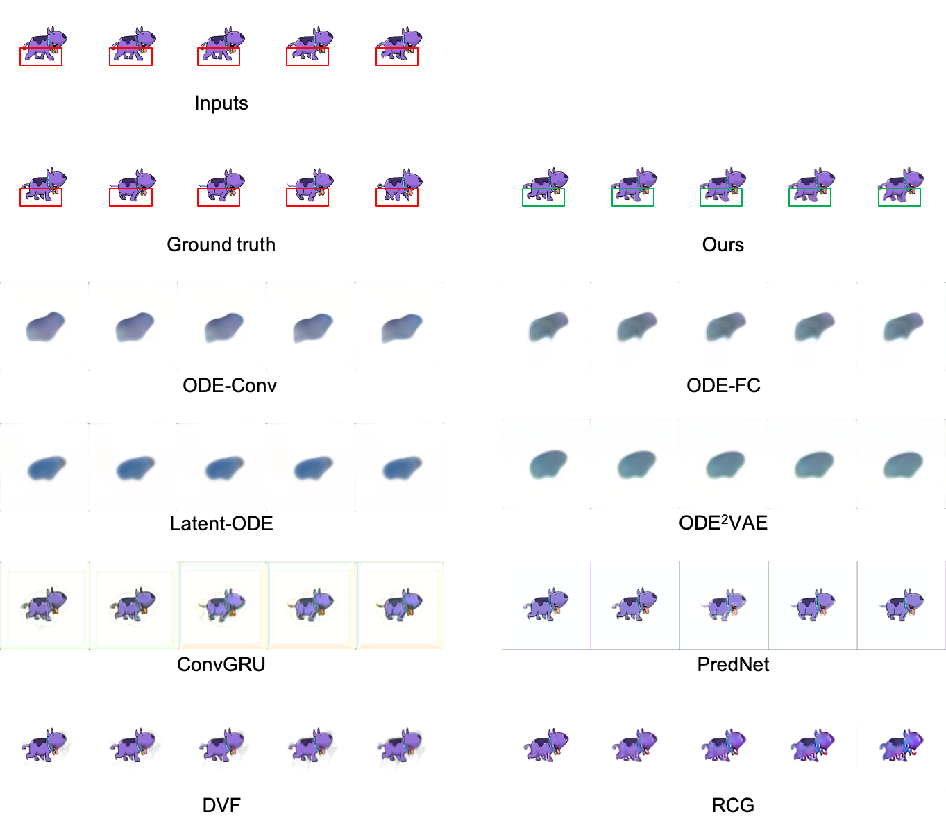
Figure 15: Qualitative comparisons with extrapolation baselines on the Moving GIF dataset.

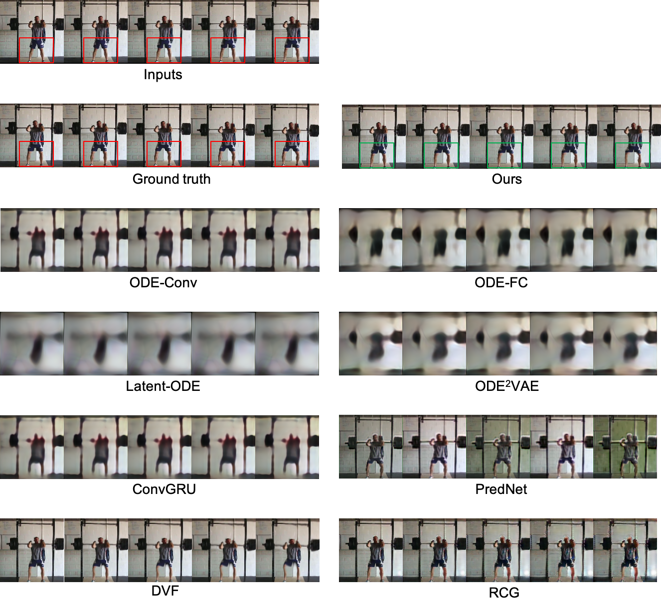
Figure 16: Qualitative comparisons with extrapolation baselines on the Penn Action dataset.

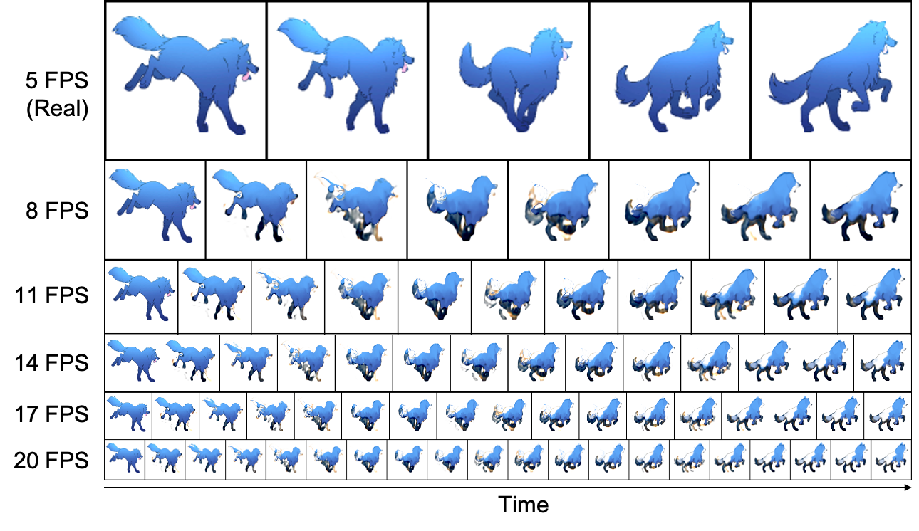
Figure 17: Generated video frames in diverse time intervals based on a 5-FPS input video with the Moving GIF dataset. (Top row: Input to Vid-ODE. Remaining rows: Videos generatedin various FPS between the start frame and the end frame.)

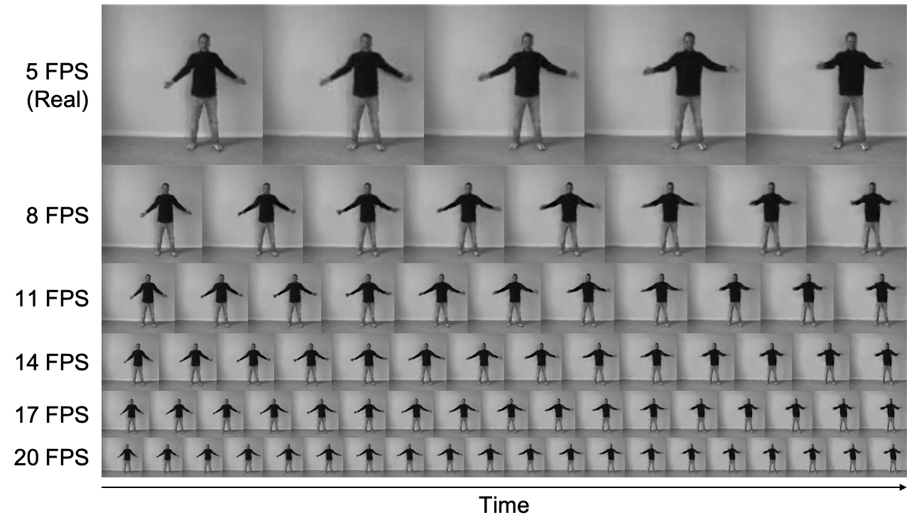
Figure 18: Generated video frames in diverse time intervals based on a 5-FPS input video with the KTH Action dataset. (Top row: Input to Vid-ODE. Remaining rows: Videos generated in various FPS between the start frame and the end frame.)

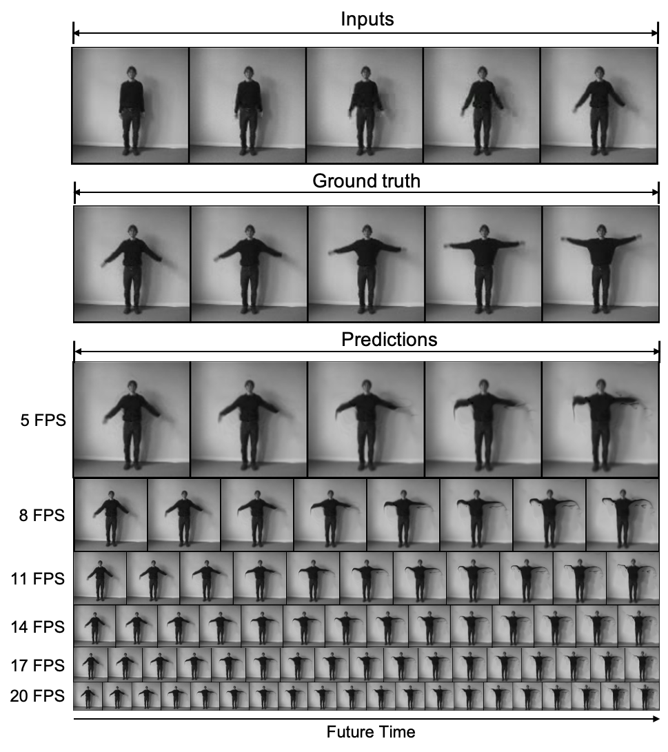
Figure 19: Based on a 5-FPS input video of the KTH Action dataset, predicting and extrapolating video frames generated in diverse time intervals. (First row: Input to Vid-ODE. Second row: Ground truth frames. Remaining rows: Predicted or extrapolated frames in various FPS.)

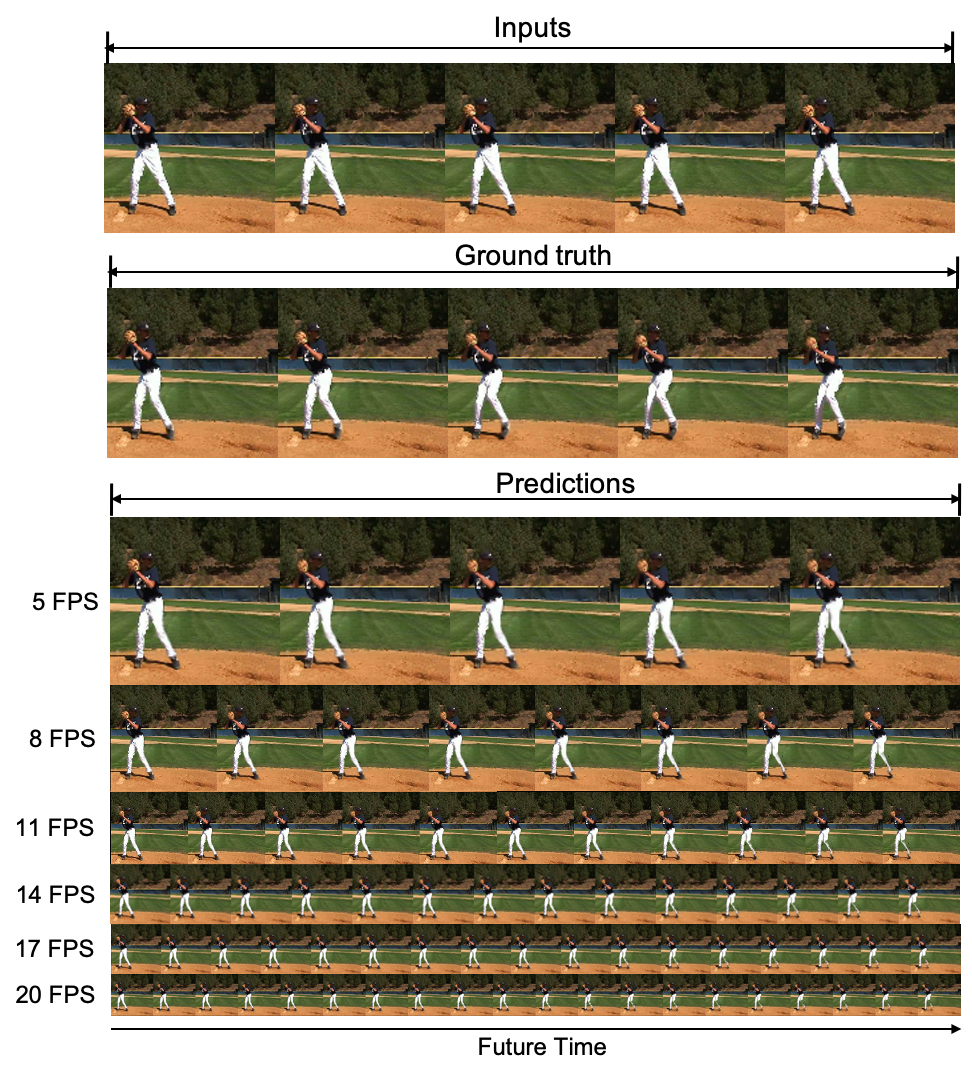
Figure 20: Based on a 5-FPS input video of the Penn Action dataset, predicting and extrapolating video frames in diverse time intervals. (First row: Input to Vid-ODE. Second row: Ground truth frames. Remaining rows: Predicted or extrapolated frames in various FPS.)

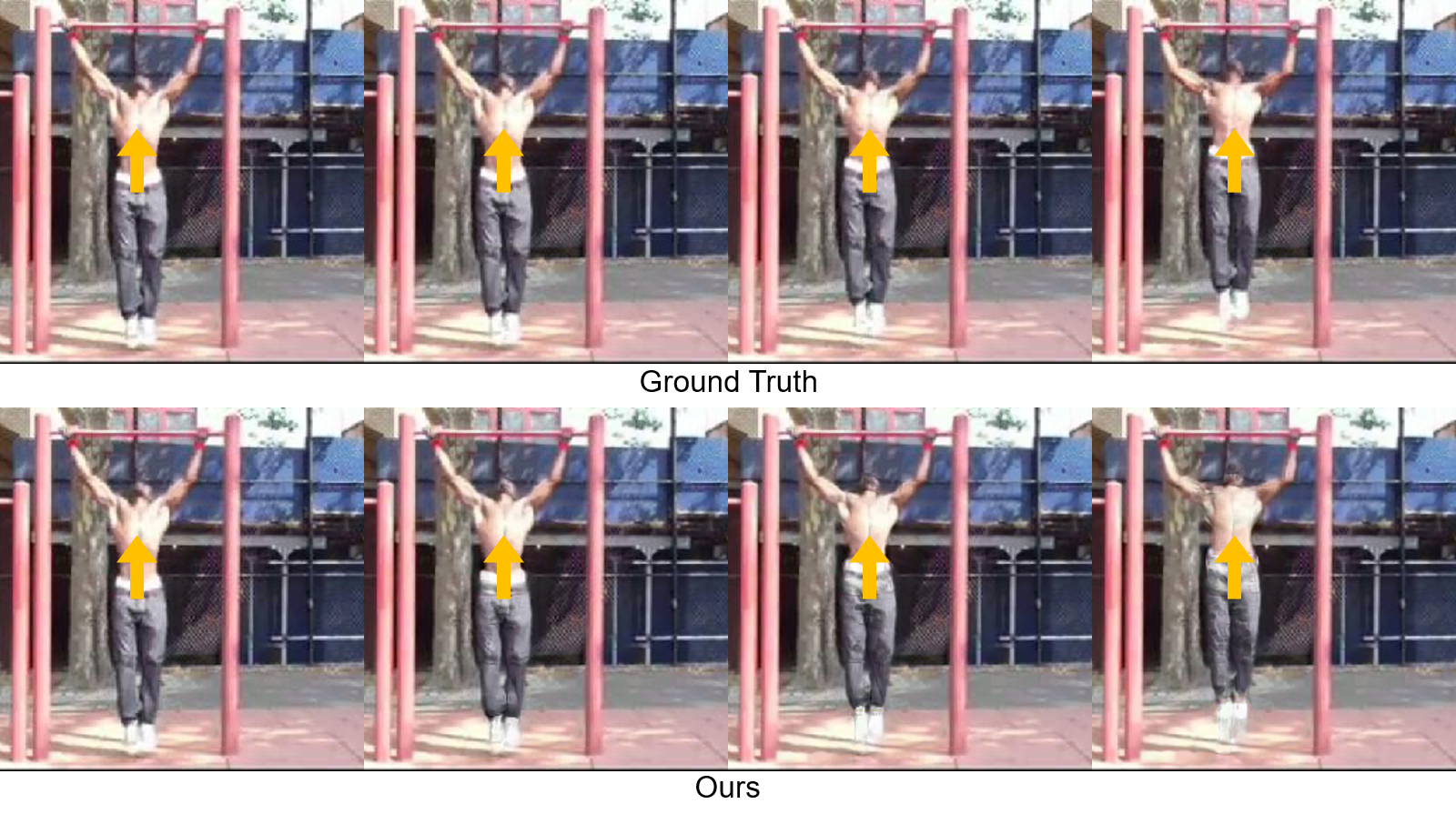
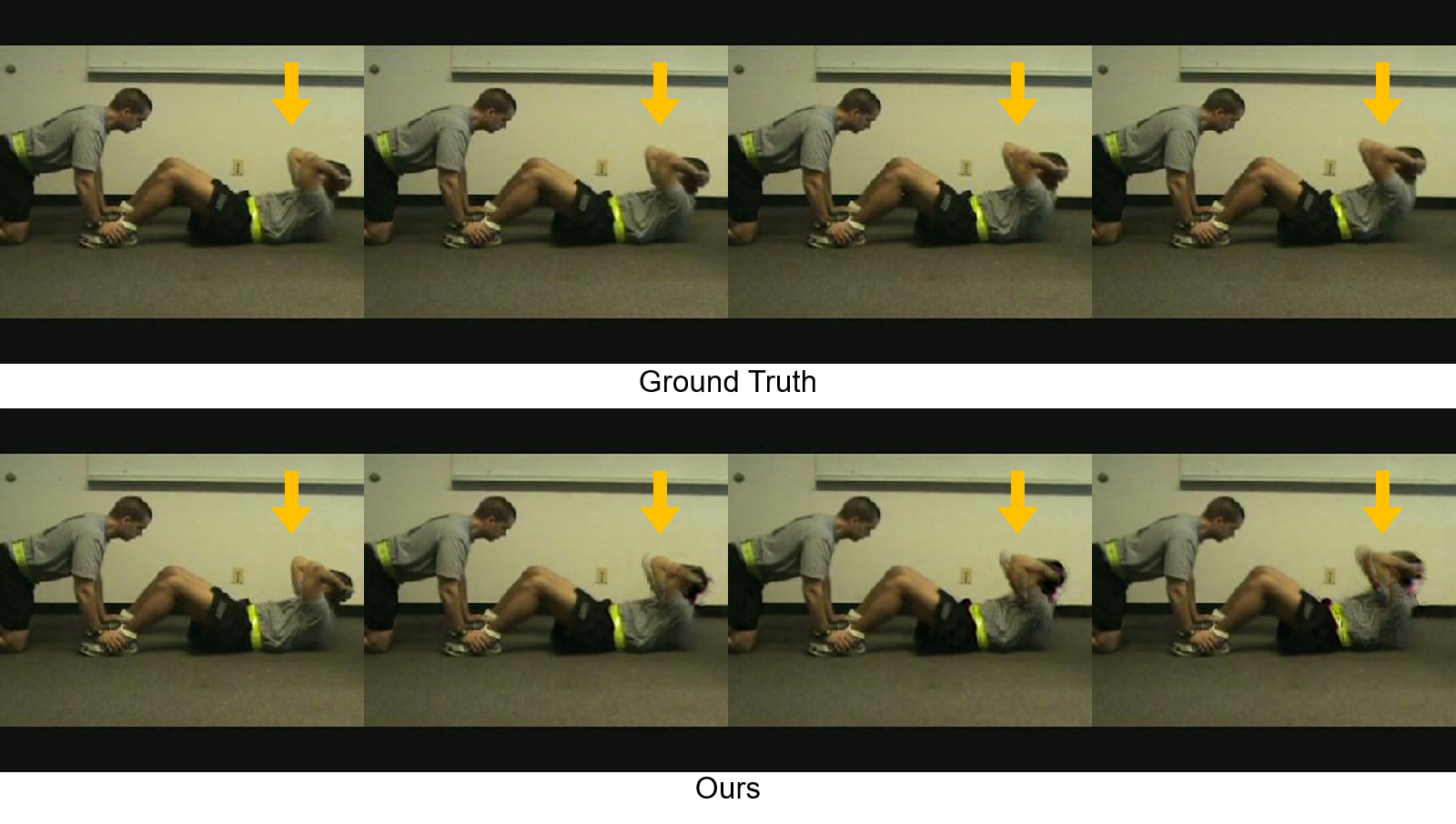
Figure 21: $256\times 256$ resolution video interpolation results with Penn Action dataset.

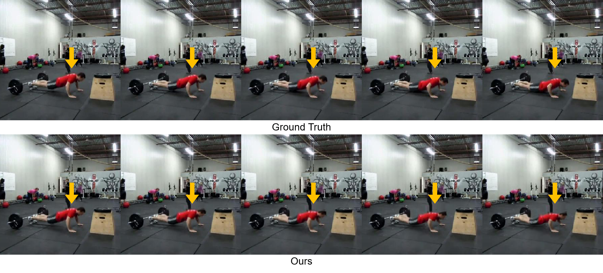
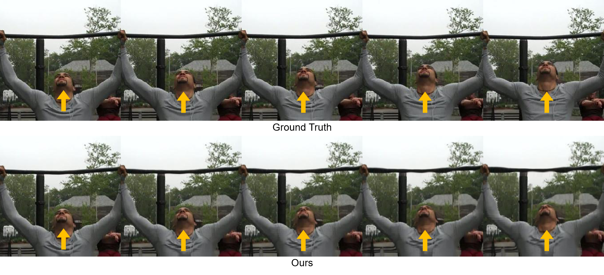
Figure 22: $256\times 256$ resolution video extrapolation results with Penn Action dataset.

References

- Ballas et al. [2015] Ballas, N.; Yao, L.; Pal, C.; and Courville, A. 2015. Delving deeper into convolutional networks for learning video representations. arXiv:1511.06432 .
- Bao et al. [2019] Bao, W.; Lai, W.-S.; Ma, C.; Zhang, X.; Gao, Z.; and Yang, M.-H. 2019. Depth-aware video frame interpolation. In Proc. of the IEEE Conference on Computer Vision and Pattern Recognition (CVPR).
- Che et al. [2018] Che, Z.; Purushotham, S.; Cho, K.; Sontag, D.; and Liu, Y. 2018. Recurrent neural networks for multivariate time series with missing values. Scientific reports 8(1): 1–12.
- Chen et al. [2018] Chen, T. Q.; Rubanova, Y.; Bettencourt, J.; and Duvenaud, D. K. 2018. Neural ordinary differential equations. In Advances in Neural Information Processing Systems (NIPS).
- De Brouwer et al. [2019] De Brouwer, E.; Simm, J.; Arany, A.; and Moreau, Y. 2019. GRU-ODE-Bayes: Continuous modeling of sporadically-observed time series. In Advances in Neural Information Processing Systems (NIPS).
- Denton and Fergus [2018] Denton, E.; and Fergus, R. 2018. Stochastic Video Generation with a Learned Prior. In International Conference on Machine Learning, 1174–1183.
- Dosovitskiy et al. [2015] Dosovitskiy, A.; Fischer, P.; Ilg, E.; Hausser, P.; Hazirbas, C.; Golkov, V.; Van Der Smagt, P.; Cremers, D.; and Brox, T. 2015. FlowNet: Learning optical flow with convolutional networks. In Proc. of the IEEE International Conference on Computer Vision (ICCV).
- Dupont, Doucet, and Teh [2019] Dupont, E.; Doucet, A.; and Teh, Y. W. 2019. Augmented neural ODEs. In Advances in Neural Information Processing Systems (NIPS).
- Franceschi et al. [2020] Franceschi, J.-Y.; Delasalles, E.; Chen, M.; Lamprier, S.; and Gallinari, P. 2020. Stochastic Latent Residual Video Prediction. arXiv preprint arXiv:2002.09219 .
- Gao et al. [2019] Gao, H.; Xu, H.; Cai, Q.-Z.; Wang, R.; Yu, F.; and Darrell, T. 2019. Disentangling propagation and generation for video prediction. In Proc. of the IEEE International Conference on Computer Vision (ICCV).
- Hao, Huang, and Belongie [2018] Hao, Z.; Huang, X.; and Belongie, S. 2018. Controllable video generation with sparse trajectories. In Proc. of the IEEE Conference on Computer Vision and Pattern Recognition (CVPR).
- Ilg et al. [2017] Ilg, E.; Mayer, N.; Saikia, T.; Keuper, M.; Dosovitskiy, A.; and Brox, T. 2017. Flownet 2.0: Evolution of optical flow estimation with deep networks. In Proc. of the IEEE Conference on Computer Vision and Pattern Recognition (CVPR).
- Jiang et al. [2018] Jiang, H.; Sun, D.; Jampani, V.; Yang, M.-H.; Learned-Miller, E.; and Kautz, J. 2018. Super slomo: High quality estimation of multiple intermediate frames for video interpolation. In Proc. of the IEEE Conference on Computer Vision and Pattern Recognition (CVPR).
- Kim et al. [2019] Kim, S.; Park, S.; Chung, S.; Lee, J.; Lee, Y.; Kim, H.; Prabhat, M.; and Choo, J. 2019. Learning to Focus and Track Extreme Climate Events. In Proc. of the British Machine Vision Conference (BMVC).
- Kingma and Ba [2014] Kingma, D. P.; and Ba, J. 2014. Adam: A method for stochastic optimization. arXiv:1412.6980 .
- Kwon and Park [2019] Kwon, Y.-H.; and Park, M.-G. 2019. Predicting future frames using retrospective cycle GAN. In Proc. of the IEEE Conference on Computer Vision and Pattern Recognition (CVPR).
- Lee et al. [2018] Lee, A. X.; Zhang, R.; Ebert, F.; Abbeel, P.; Finn, C.; and Levine, S. 2018. Stochastic adversarial video prediction. arXiv preprint arXiv:1804.01523 .
- Liang et al. [2017] Liang, X.; Lee, L.; Dai, W.; and Xing, E. P. 2017. Dual motion GAN for future-flow embedded video prediction. In Proc. of the IEEE International Conference on Computer Vision (ICCV).
- Liu et al. [2017] Liu, Z.; Yeh, R. A.; Tang, X.; Liu, Y.; and Agarwala, A. 2017. Video frame synthesis using deep voxel flow. In Proc. of the IEEE International Conference on Computer Vision (ICCV).
- Lotter, Kreiman, and Cox [2016] Lotter, W.; Kreiman, G.; and Cox, D. 2016. Deep predictive coding networks for video prediction and unsupervised learning. arXiv:1605.08104 .
- Mao et al. [2017] Mao, X.; Li, Q.; Xie, H.; Lau, R. Y.; Wang, Z.; and Paul Smolley, S. 2017. Least squares generative adversarial networks. In Proc. of the IEEE International Conference on Computer Vision (ICCV).
- Reda et al. [2019] Reda, F. A.; Sun, D.; Dundar, A.; Shoeybi, M.; Liu, G.; Shih, K. J.; Tao, A.; Kautz, J.; and Catanzaro, B. 2019. Unsupervised Video Interpolation Using Cycle Consistency. In Proc. of the IEEE International Conference on Computer Vision (ICCV).
- Revaud et al. [2015] Revaud, J.; Weinzaepfel, P.; Harchaoui, Z.; and Schmid, C. 2015. Epicflow: Edge-preserving interpolation of correspondences for optical flow. In Proc. of the IEEE Conference on Computer Vision and Pattern Recognition (CVPR).
- Rubanova, Chen, and Duvenaud [2019] Rubanova, Y.; Chen, T. Q.; and Duvenaud, D. K. 2019. Latent Ordinary Differential Equations for Irregularly-Sampled Time Series. In Advances in Neural Information Processing Systems (NIPS).
- Schuldt, Laptev, and Caputo [2004] Schuldt, C.; Laptev, I.; and Caputo, B. 2004. Recognizing human actions: a local SVM approach. In Proc. of the International Conference on Pattern Recognition (ICPR).
- Siarohin et al. [2019] Siarohin, A.; Lathuilière, S.; Tulyakov, S.; Ricci, E.; and Sebe, N. 2019. Animating arbitrary objects via deep motion transfer. In Proc. of the IEEE Conference on Computer Vision and Pattern Recognition (CVPR).
- Wang et al. [2019a] Wang, Y.; Jiang, L.; Yang, M.-H.; Li, L.-J.; Long, M.; and Fei-Fei, L. 2019a. Eidetic 3d LSTM: A model for video prediction and beyond. In Proc. of the International Conference on Learning Representations (ICLR).
- Wang et al. [2017] Wang, Y.; Long, M.; Wang, J.; Gao, Z.; and Philip, S. Y. 2017. Predrnn: Recurrent neural networks for predictive learning using spatiotemporal lstms. In Advances in Neural Information Processing Systems (NIPS).
- Wang et al. [2019b] Wang, Y.; Zhang, J.; Zhu, H.; Long, M.; Wang, J.; and Yu, P. S. 2019b. Memory In Memory: A Predictive Neural Network for Learning Higher-Order Non-Stationarity from Spatiotemporal Dynamics. In Proc. of the IEEE Conference on Computer Vision and Pattern Recognition (CVPR).
- Wang et al. [2004] Wang, Z.; Bovik, A. C.; Sheikh, H. R.; and Simoncelli, E. P. 2004. Image quality assessment: from error visibility to structural similarity. IEEE transactions on image processing 13(4): 600–612.
- Xingjian et al. [2015] Xingjian, S.; Chen, Z.; Wang, H.; Yeung, D.-Y.; Wong, W.-K.; and Woo, W.-c. 2015. Convolutional LSTM network: A machine learning approach for precipitation nowcasting. In Advances in Neural Information Processing Systems (NIPS).
- Yildiz, Heinonen, and Lahdesmaki [2019] Yildiz, C.; Heinonen, M.; and Lahdesmaki, H. 2019. ODE2VAE: Deep generative second order ODEs with Bayesian neural networks. In Advances in Neural Information Processing Systems (NIPS).
- Zhang et al. [2018] Zhang, R.; Isola, P.; Efros, A. A.; Shechtman, E.; and Wang, O. 2018. The unreasonable effectiveness of deep features as a perceptual metric. In Proc. of the IEEE Conference on Computer Vision and Pattern Recognition (CVPR).
- Zhang, Zhu, and Derpanis [2013] Zhang, W.; Zhu, M.; and Derpanis, K. G. 2013. From actemes to action: A strongly-supervised representation for detailed action understanding. In Proc. of the IEEE International Conference on Computer Vision (ICCV).