Who’s in the Gang? Revealing Coordinating Communities in Social Media

Abstract

Political astroturfing and organised trolling are online malicious behaviours with significant real-world effects. Common approaches examining these phenomena focus on broad campaigns rather than the small groups responsible. To reveal latent networks of cooperating accounts, we propose a novel temporal window approach that relies on account interactions and metadata alone. It detects groups of accounts engaging in behaviours that, in concert, execute different goal-based strategies, which we describe. Our approach is validated against two relevant datasets with ground truth data.

1 Introduction

Online social networks (OSNs) have established themselves as flexible and accessible systems for activity coordination and information dissemination. This benefit was illustrated during the Arab Spring [1] but its danger continues in ongoing political interference [2, 3, 4]. Modern information campaigns are participatory, using the audience to amplify the desired narrative [5]. Through cyclical reporting, social media users can unknowingly become “unwitting agents” as “sincere activists” of state-based operations [6]. The use of political bots to influence the framing and discussion of issues in the mainstream media (MSM) remains prevalent [7, 8, 2]. This megaphone effect requires coordinated action and a degree of regularity that may leave traces in the digital record.

Relevant research has focused on high level analyses of campaign detection and classification [9, 10, 11], the identification of botnets and other dissemination groups [12, 13, 8], and coordination at the community level [14, 15]. Some have considered generalised approaches to social media analytics [16, 17, 18], but unanswered questions regarding the clarification of coordination strategies remain.

We present a new approach to detect groups engaging in potentially coordinated activities, revealed through anomalous levels of coincidental behaviour. Links in the groups are inferred from behaviours that, with intent, are used to execute a number of identifiable coordination strategies. We validate our new technique on various datasets and show it successfully identifies coordinating communities.

Our approach infers ties between accounts based on activity to construct latent connection networks (LCNs), in which highly coordinating communities (HCCs) are detected. We use a variant of focal structures analysis (FSA) [19] to do this. A window-based approach is used to enforce temporal constraints.

Comparison of two relevant datasets, including labeled ground truth, with a randomised dataset provides validation. These research questions guided our evaluation:

RQ1

How can HCCs be found in an LCN?

RQ2

How do the discovered communities differ?

RQ3

Are the HCCs internally or externally focused?

RQ4

How consistent is the HCC messaging?

This paper provides an overview of relevant literature, followed by a discussion of online coordination strategies and their execution. Our approach is then explained, and its experimental validation is presented.

1.1 Related Work

Sociological studies of influence campaigns can reveal their intent and how they are conducted. Starbird et al. [5] highlight three kinds: orchestrated, centrally controlled campaigns (e.g., paid teams [20, 21]); cultivated campaigns that infiltrate existing movements; and emergent campaigns arising from shared ideology (e.g., groups around conspiracists). Though their strategies differ, they use the same online interactions as normal users, but their patterns differ.

Computer science has focused on detecting information operations on social media via automation [22], campaign detection [9, 23, 10, 11], temporal patterns [24], and community detection [25, 12, 13]. Other studies have explored how bots and humans interact in political settings [7, 2], including exploring how deeply embedded bots appear in the network and their degree of organisation [8]. There is, however, a research gap: the computer science study of the “orchestrated activities” of accounts in general, regardless of their degree of automation [26, 11].

Though some studies have observed the existence of strategic behaviour in and between online groups (e.g., [4, 14, 15]), the challenge of identifying a broad range of strategies and their underpinning execution methods remains.

Inferring social networks from OSN data requires attendance to the temporal aspect to understand information (and influence) flow and degrees of activity [27]. Real time processing of OSN posts can enable tracking narratives via text clusters [28], but to process networks requires graph streams [29] or window-based pipelines (e.g., [17, 18]).

This work contributes to the identification of strategic coordination behaviours, along with a general technique to enable detection of groups using them.

2 Coordination Strategies

Online influence relies on two primary mechanisms: dissemination and engagement. For example, an investigation of social media activity following UK terrorist attacks in 2017 identified accounts promulgating contradictory narratives, inflaming racial tensions and simultaneously promoting tolerance to sow division. By engaging aggressively, the accounts drew in participants who then spread the message.

Dissemination aims to maximise audience, to convince through repeated exposure and, in the case of malicious use, to cause outrage, polarisation and confusion, or at least attract attention to distract from other content.

Engagement is a subset of dissemination that solicits a response. It relies on targeting individuals or communities through mentions, replies and the use of hashtags as well as rhetorical approaches that invite responses (e.g., inflammatory comments or, as present in the UK terrorist example above, pleas to highly popular accounts).

A number of online coordination strategies have been observed in the literature making use of both dissemination and engagement, including:

1. Pollution: flooding a community with repeated or objectionable content, causing the OSN to shut it down [30, 15];

2. Boost: heavily reposting content to make it appear popular [23, 12, 13];

3. Bully: groups of individuals harassing another individual or community [31, 14]; and

4. Metadata Shuffling: groups of accounts changing metadata to hide their identities [32, 3].

Different behaviour primitives (e.g., Table 1) can be used to execute these strategies. Dissemination can be carried out by reposting, using hashtags, or mentioning highly connected individuals in the hope they spread a message further. Accounts doing this covertly will avoid direct connections, and thus inference is required for identification. Giglietto et al. [33] propose detecting anomalous levels of coincidental URL use as a way to do this; we expand this approach to other interactions.

Some strategies require more sophisticated detection: detecting bullying through dogpiling (e.g., during the #GamerGate incident [31]) requires collection of (mostly) entire conversation trees, which, while trivial to obtain on forum-based sites (e.g., Facebook and Reddit), are difficult on stream-of-post sites (e.g., Twitter, Parler and Gab). Detecting metadata shuffling requires long term collection on broad issues to detect the same accounts being active in different contexts.

3 Methodology

The major OSNs share a number of features, primarily in how they permit users to interact. By focusing on these commonalities, it is possible to develop approaches that generalise across the OSNs that offer them.

Traditional social network analysis relies on long-standing relationships between actors. On OSNs these are typically friend/follower relations. These are expensive to collect and quickly degrade in meaning if not followed with frequent activity. By focusing on active interactions, it is possible to understand not just who is interacting with whom, but to what degree. This provides a basis for constructing (or inferring) social networks, acknowledging they may be transitory.

LCNs are built from inferred links between accounts. Supporting criteria include retweeting the same tweet (co-retweet), using the same hashtags (co-hashtag) or URLs (co-URL), mentioning the same accounts (co-mention), or joining the same ‘conversation’ (a tree of reply chains with a common root tweet) (co-conv).

Table 1: Social media interaction equivalents

OSN	POST	REPOST	REPLY	MENTION	TAG	LIKE
Twitter	tweet	retweet	reply tweet	@mention	#hashtags	favourite
Facebook	post	share	comment	mention	#hashtag	reactions
Tumblr	post	repost	comment	@mention	#tag	heart
Reddit	post	crosspost	comment	/u/mention	subreddit	up/down vote

3.1 The LCN / HCC Pipeline

The key steps to extract HCCs from raw social media data are shown in Figure 1.

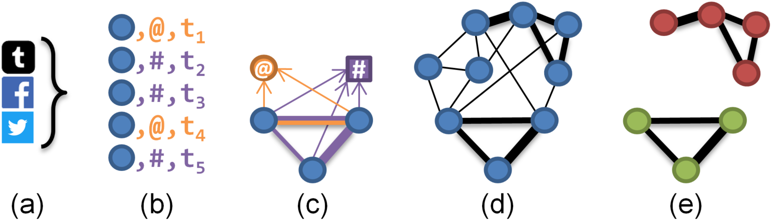
Figure 1: Conceptual LCN construction and HCC discovery process.

Step 1. Convert social media posts $P$ to common interaction primitives, $I_{all}$. This step removes extraneous data and provides an opportunity for the fusion of sources.

Step 2. From $I_{all}$, filter the interactions, $I_{C}$, relevant to the set $C$=$\{c_{1},c_{2},...,c_{q}\}$ of criteria (e.g., co-mentions and co-hashtags). Illustrated in Figure 1b are the filtered mentions (in orange) and hashtag uses (in purple), ordered according to timestamp.

Step 3. Infer links between accounts given $C$, ensuring links are typed by criterion. The result, $M$, is a collection of inferred pairings. The count of inferred links between accounts $u$ and $v$ due to criterion $c\in C$ is $\beta^{c}_{\{u,v\}}$. Figure 1c shows inferred links between accounts due to common interactions.

Step 4. Construct an LCN, $L$, from the pairings in $M$. This network $L$=$(V,E)$ is a set of vertices $V$ representing accounts connected by weighted edges $E$ of inferred links. These edges represent evidence of different criteria linking the adjacent vertices. The weight of each edge $e_{\{u,v\}}\in E$ between vertices representing $u$ and $v$ for each criterion $c$ is $w^{c}_{\{u,v\}}$, and is equal to $\beta^{c}_{\{u,v\}}$.

Some community detection algorithms will require the multi-edges be collapsed to single edges, however, the edge weights are incomparable (e.g., retweeting the same tweet is not equivalent to using the same hashtag). For practical purposes, the inferred links can be collapsed and the weights combined for cluster detection using a simple summation, e.g., Equation (1), or a more complex process like varied criteria weighting. Implementations can retain information about how the edges were collapsed for later analysis, but the lack of multi-edges permits scope for more community detection algorithms to be used.

$$w_{\{u,v\}}=\sum_{c=1}^{q}w^{c}_{\{u,v\}}$$ (1)

Some criteria may result in highly connected LCNs, even if its members never directly interact. The final step filters out these coincidental connections.

Step 5. Identify the highest coordinating communities, $H$, in $L$ (Figure 1e), using FSA_V (Algorithm 1), a variant of FSA [19], or an alternative community detection algorithm, merging multi-edges as required. FSA_V divides $L$ into communities using the Louvain algorithm [34] and builds candidate HCCs within each, starting with the ‘heaviest’ (i.e., highest weight) edge (representing the most evidence of coordination). It then attaches the next heaviest edge until the candidate’s mean edge weight (MEW) is no less than $\theta$ ($0<\theta\leq 1$) of the previous candidate’s MEW, or is less than $L$’s overall MEW. In testing, edge weights appeared to follow a power law, so $\theta$ was introduced to identify the point at which the edge weight drops significantly; $\theta$ requires tuning. A final filter ensures no HCC with a MEW less than $L$’s is returned. Unlike in FSA [19], recursion is not used, nor stitching of candidates, resulting in a simpler algorithm.

Algorithm 1 Extract HCCs (FSA_V)

Input: $L$=$(V,E)$: An LCN, $\theta$: HCC threshold
Output: $H$: Highly coordinating communities

1:  $E^{\prime}\leftarrow\text{MergeMultiEdges}(E)$

2:  $g\_mean\leftarrow\text{MeanWeight}(E^{\prime})$

3:  $louvain\_communities\leftarrow\text{ApplyLouvain}(L)$

4:  Create new list, $H$

5:  for $l\in louvain\_communities$ do

6:     Create new community candidate, $h=(V_{h},E_{h})$

7:     Add heaviest edge $e\in l$ to $h$

8:     $growing\leftarrow$ true

9:     while $growing$ do

10:        Find heaviest edge $\vec{e}\in l$ connected to $h$ not in $h$

11:        $old\_mean\leftarrow\text{MeanWeight}(E_{h})$

12:        $new\_mean\leftarrow\text{MeanWeight}(\text{Concatenate}(E_{h},\vec{e}))$

13:        if $new\_mean<g\_mean$ or $new\_mean<(old\_mean\times\theta)$ then

14:           $growing\leftarrow$ false

15:        else

16:           Add $\vec{e}$ to $h$

17:     if MeanWeight$(E_{h})>g\_mean$ then

18:        Add $h$ to $H$

This algorithm prioritises edge weights while maintaining an awareness of the network topology by examining adjacent edges, something ignored by simple edge weight filtering. Our goal is to find sets of strongly coordinating users, so it is appropriate to prioritise strongly tied communities while still acknowledging coordination can also be achieved with weak ties (e.g., $100$ accounts paid to retweet a single tweet).

The complexity of the entire pipeline is low order polynomial, O($n^{2}$), due primarily to the pairwise comparison of accounts to infer links in Step $3$, which is constrained by window size when addressing the temporal aspect. Community detection algorithms designed for large networks may help to address this limitation [35].

3.2 Addressing the Temporal Aspect

Temporal information is a key element of coordination, and thus is critical for effective coordination detection. Frequent posts within a short period may represent genuine discussion or deliberate attempts to game trend algorithms [26, 10, 28]. We treat the post stream as a series of discrete windows to constrain detection periods. An LCN is constructed from each window (Step 4), and these are then aggregated and mined for HCCs (Step 5). As we assume posts arrive in order, their timestamp metadata can be used to sort and assign them to windows.

4 Evaluation and Validation

Our approach was evaluated by searching for Boost by co-retweet and other strategies in two datasets, while varying window sizes ($\gamma$). FSA_V was compared against two other community detection algorithms when applied to the LCNs built in Step 4 (aggregated). We then validated the resulting HCCs through content, temporal and network analysis.

Table 2: Dataset statistics

	Tweets (T)	Retweets (RT)		Accounts	T / Account / Day	RT / Account / Day
DS1	115,913	63,164	(54.5%)	20,563	0.31	0.17
- GT	4,193	2,505	(59.7%)	134	1.74	1.04
DS2	1,571,245	729,937	(56.5%)	1,381	3.12	1.45

4.1 The Datasets

The two real-world datasets selected (Table 2) represent two primary collection techniques: filtering a stream of posts using keywords direct from the OSN (DS1) and collecting the posts of specific accounts (DS2):

DS1

Tweets relating to a regional Australian election in March 2018, including a ground truth subset (GT); and

DS2

A large subset of the Internet Research Agency (IRA) dataset published by Twitter in October 2018.

The data were collected, held and analysed in accordance with an approved ethics protocol.

DS1 was collected using RAPID [16] over an 18 day period (the election was on day 15) in March 2018. The filter terms included nine hashtags and $134$ political handles (candidate and party accounts). The dataset was expanded by retrieving all replied to, quoted and political account tweets posted during the collection period. The political account tweets formed our ground truth.

The IRA tweets cover 2009 to 2018, but DS2 consists of all posted in 2016, the year of the US Presidential election. Because DS2 consists entirely of IRA accounts [20], it was expected to include evidence of cooperation.

4.2 Set Up

Window size $\gamma$ was set at $\{15,60,360,1440\}$ (in minutes) and the three community detection methods used on the aggregated LCNs were:

• FSA_V ($\theta$=$0.3$);

• k nearest neighbour (kNN) with $k$=$ln(|V|)$ (cf. [23]);

• a simple threshold retaining the heaviest $90\%$ of edges.

Values for $\theta$ and the threshold were based on experimenting with values in $[0.1,0.9]$, maximising the MEW to HCC size ratio, using the $\gamma$=$\{15,1440\}$ DS1 and DS2 aggregated LCNs. Values for $\gamma$ were based on Zhao et al.’s [36] observation that 75% of retweets occur within six hours of posting. This implies that if attempts were made to boost a tweet, retweeting it in much shorter times would be required for it to stand out from typical traffic. Varol et al. [10] checked Twitter’s trending hashtags every $10$ minutes, so values chosen for $\gamma$ ranged from 15m to a day, growing by a factor of approximately four at each increment. Coordinated retweeting was expected to occur in the smaller windows, but then replaced by coincidental co-retweeting as the window size increases.

4.3 Results

The research questions introduced in Section 1 guide our discussion, but we also present follow-up analyses.

4.3.1 HCC Detection (RQ1)

Detecting different strategies. The three detection methods all detected HCCs when searching for Boost (co-retweets), Pollute (co-hashtags), and Bully (co-mentions) (Table 3). Notably, kNN consistently builds a single large HCC, highlighting the need to filter the network prior to applying it (cf. [23]). The kNN HCC is also consistently nearly as large as the original LCN for DS2, perhaps due to the low number of accounts and the fact that every edge of the retained vertices is retained, regardless of weight. It is not clear, then, that kNN is producing meaningful results, even if it can extract a community.

Table 3: HCCs by coordination strategy

			GT			DS1			DS2
	Strategy	$\gamma$	Nodes	Edges	Comp.	Nodes	Edges	Comp.	Nodes	Edges	Comp.
LCN	Boost	15	44	112	5	8,855	80,702	419	855	23,022	14
	Pollute	15	51	154	2	13,831	1,281,134	73	1,203	65,949	5
	Bully	60	70	482	1	16,519	1,925,487	222	1,103	37,368	5
FSA_V	Boost	15	9	6	3	633	753	167	113	758	19
	Pollute	15	9	5	4	135	93	50	24	15	9
	Bully	60	11	7	4	338	280	119	109	1,123	16
kNN	Boost	15	9	21	1	1,041	33,621	1	675	22,494	1
	Pollute	15	11	37	1	724	153,424	1	1,040	65,280	1
	Bully	60	18	135	1	1,713	663,413	1	692	35,136	1
Threshold	Boost	15	11	16	3	85	68	31	8	10	2
	Pollute	15	24	26	3	44	37	10	6	13	1
	Bully	60	15	19	3	25	23	8	10	10	3

Varying window size. Different strategies may be executed over different time periods, based on their aims. Boosting a message to game trending algorithms requires the messages to appear close in time, whereas some forms of Bullying exhibit only consistency and low variation (mentioning the same account repeatedly). Polluting a user’s timeline on Twitter can also be achieved by frequently joining their conversations over a sustained period. Varying $\gamma$ searching for Boost, we found different accounts were prominent over different timeframes (Table 4); the overlap in the accounts detected in each timeframe differed considerably even though the number of HCCs stayed relatively similar. HCC sizes seemed to follow a power law; most were very small but a few were large.

Table 4: HCCs by window size $\gamma$ (Boost, FSA_V)

		Graph Attributes			HCC Sizes		Nodes in common
	$\gamma$	Nodes	Edges	HCCs	Min.	Max.	$\gamma$=15	$\gamma$=60	$\gamma$=360	$\gamma$=1440
DS1	15	633	753	167	2	18	633	218	93	100
	60	619	1,293	151	2	13	-	619	208	193
	360	503	1,119	127	2	19	-	-	503	350
	1440	815	2,019	141	2	110	-	-	-	815
DS2	15	113	758	19	2	65	113	34	29	25
	60	77	394	18	2	27	-	77	62	54
	360	98	775	15	2	32	-	-	98	56
	1440	69	380	15	2	27	-	-	-	69

HCC detection methods. Similarly, HCCs discovered by the three community extraction methods (Table 5) exhibit large discrepancies, suggesting that whichever method is used, tuning is required to produce interpretable results. This is evident in the literature: Cao et al. conducted significant pre-processing when identifying URL sharing campaigns [23], and Pacheco et al. showed how specific strategies could identify groups in the online narrative surrounding the Syrian White Helmet organisation [37]. Here we present the variation in results while controlling methods and other variables and keeping the coordination strategy constant, as our focus is the effectiveness of the method.

Table 5: HCCs by detection method (Boost, $\gamma$=$15$)

		Graph Attributes			HCC Sizes		Nodes in common
		Nodes	Edges	HCCs	Min.	Max.	FSA_V	$kNN$	Threshold
DS1	FSA_V	633	753	167	2	18	633	56	36
	kNN	1,041	33,621	1	1,041	1,041	-	1,041	44
	Threshold	85	68	31	2	14	-	-	85
DS2	FSA_V	113	758	19	2	65	113	88	4
	kNN	675	22,494	1	675	675	-	675	8
	Threshold	8	10	2	2	6	-	-	8

4.3.2 HCC Differentiation (RQ2)

How similar are the discovered HCCs to each other and to the rest of the corpus? The HCC detection methods used relied on network information; in contrast we examine content, metadata and temporal information to validate the results. We contrast DS1 and DS2 results with GT (cf. [4]) and a RANDOM dataset (cf. [23]), constructed by randomly assigning non-HCC accounts from DS1 to groups matching the distribution of its HCCs (FSA_V, $\gamma$=$15$). As DS2 consisted entirely of bad actors, it was felt non-HCC accounts from DS1 would be more representative of non-coordinating ‘normal’ accounts.

Internal consistency. If HCCs are boosting a message, it is reasonable to assume the content of HCCs members will be more similar internally that when compared externally, to the content of non-members. Treating each HCC member’s tweets as a single document, we created a doc-term matrix using $5$ character n-grams for terms, and then compared the members’ document vectors using cosine similarity. This approach was chosen for its performance with non-English corpora [38], and because using individual tweets as documents produced too sparse a matrix. Visualising the similarities between accounts, grouping them by HCC (Figure 2), the HCCs are discernible as being internally similar. This method ignores the number of tweets HCCs post, so we can draw no conclusions about connections between HCC size and the internal similarity of their content, though more active HCCs (i.e., with more tweets) are more likely to be similar, through co-occurrence of n-grams. The RANDOM groupings demonstrated little to no similarity, internal or external, as expected, while the DS2 HCCs demonstrated high internal similarity, as expected of organised accounts over an extended period.

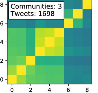
(a) GT.

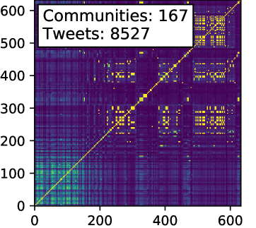
(b) DS1.

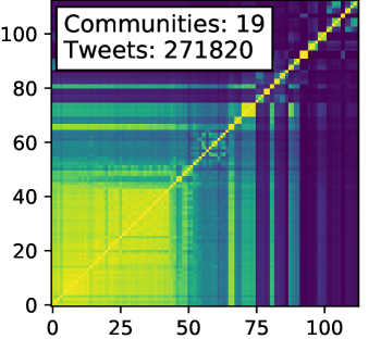
(c) DS2.

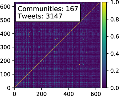
(d) RANDOM.

Figure 2: Similarity matrices of content posted by HCC accounts ($\gamma$=15, FSA_V). Each axis has an entry for each account, grouped by HCC. Each cell represents the similarity between the two corresponding accounts’ content, calculated using cosine similarity (yellow = high similarity). Each account’s content is represented as a vector of $5$ character n-grams of their combined tweets.

Temporal patterns. Campaign types exhibit different temporal patterns [9]. We used the same temporal averaging technique as Lee et al. [9] to compare the daily activities of the HCCs found in GT, DS1 and RANDOM (Figure 3a) and weekly activities in DS2 (Figure 3b). The GT accounts were clearly most active at two points prior to the election (around day $15$), during the last leaders’ debate and just prior to the mandatory electoral advertising blackout. DS1 and RANDOM HCCs were only consistently active at different times: around the day 3 leaders’ debate and on election day, respectively. Inter-HCC variation may have dragged the mean activity value down, as many small HCCs were inactive each day. Reintroducing FSA’s stitching element to FSA_V may avoid this. In DS2, HCC activity increased in the second half of 2016, culminating in a peak around the election, inflated by two very active HCCs, both of which used many predominantly benign hashtags over the year.

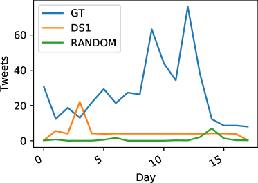
(a) GT, DS1 and RANDOM.

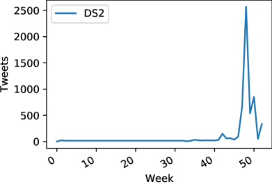
(b) DS2.

Figure 3: Averaged temporal graphs of HCC activities ($\gamma$=$15$, FSA_V).

Hashtag use. The most frequent hashtags in the most active HCCs revealed the most in GT. It is possible to assign some HCCs to political parties via the partisan hashtags (e.g., #voteliberals), although the hashtags of contemporaneous cultural events are also prominent (Figure 4a). DS1 hashtags are all politically relevant, but are dominated by a single small HCC which used many hashtags very often (Figure 4b). These accounts clearly attempted to disseminate their tweets through using $1,621$ hashtags in $354$ tweets. Similarly, DS2 hashtags were dominated by a single HCC (using $41,317$ relatively general hashtags in $40,992$ tweets) and one issue-motivated HCC (Figure 4c). Given DS2 covers an entire year, it is unsurprising that the largest HCCs use such a variety of hashtags that their hashtags do not appear on the chart.

Analysing co-occurring hashtags can help further explore the HCC discussions to determine if HCCs are truly single groups or merged ones. Applied to GT HCC activities (Figure 4a), it was possible to delineate subsets of hashtags in use: e.g., one HCC promoted a political narrative in some tweets with #orangelibs and discussed cultural events in others with #adlww (Figure 5), but was definitely one group.

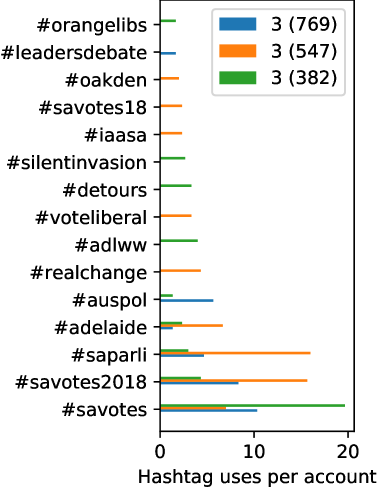
(a) GT.

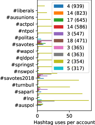
(b) DS1.

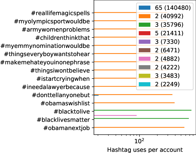
(c) DS2.

Figure 4: Most used hashtags (per account) of the most active HCCs ($\gamma$=15, FSA_V). The labels indicate member and tweet counts. Not all HCCs used a hashtag often enough to be visible.

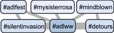
Figure 5: Cluster of hashtags, connected only when they appeared in the same tweet (GT, $\gamma$=15, FSA_V). Link width = tweet count.

Examining the Ground Truth. The importance of having ground truth in context is demonstrated by Keller et al. [4]. By analysing the actions of known bad actors in a broad dataset, they could identify not just different subteams within the actors and their strategies, but their effect on the broader discussion. Many datasets comprising only bad actors (e.g., DS2) miss this context.

Considering GT alone, the HCCs identified consist only of members within the same political party, across all values of $\gamma$. Some accounts appeared in each window size. HCCs of six major parties were identified. Examination of these HCCs’ content confirmed they were genuine.

4.3.3 Focus of connectivity (RQ3)

Groups that retweet or mention themselves create direct connections; therefore to be covert, it would be sensible to have a low internal retweet and mention ratios (IRR and IMR, respectively). Figure 6 shows IRR and IMR for the datasets. The larger the HCC size, the greater the likelihood of retweeting or mentioning internally, so it is notable that DS2’s largest HCC has IRR and IMR’s of around $0$, though even the smaller HCCs have low ratios. Ratios for the smallest HCCs seem largest, possibly due to low numbers of posts, many of which may be retweets or include a mention, inflating the ratios. The hypothesis that political accounts would retweet and mention themselves frequently is not confirmed by these results, possibly because they are retweeting and mentioning official or party accounts outside the HCCs.

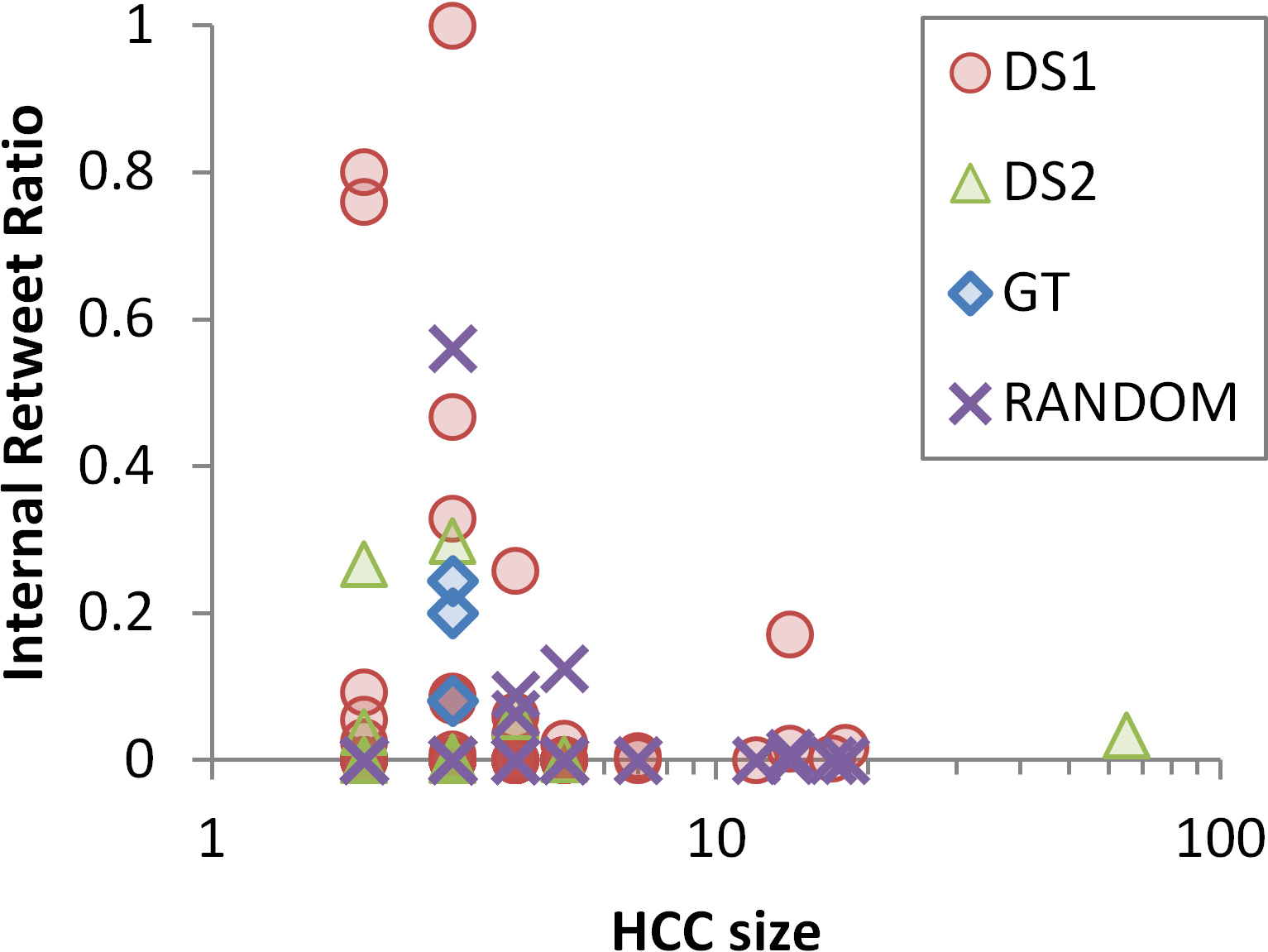
(a) Retweets.

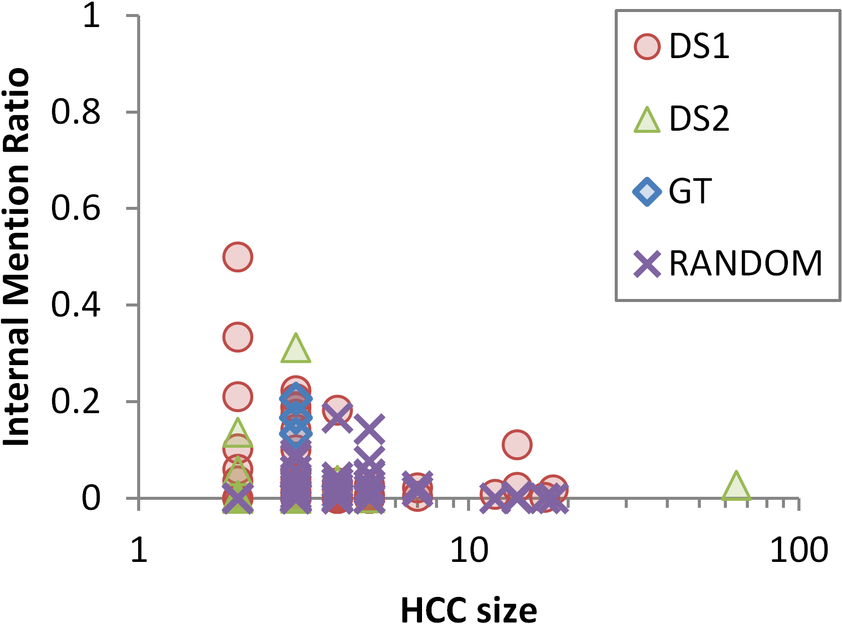
(b) Mentions.

Figure 6: The proportions of each HCCs retweets and mentions referring to accounts within the HCC ($\gamma$=15, FSA_V).

4.3.4 Content variation (RQ4)

Highly coordinated reposting involved reusing the same content frequently, resulting in low feature variation (e.g., hashtags, URLs, mentioned accounts), which can be measured as entropy [23]. A frequency distribution of each HCC’s use of each feature type was used to calculate each entropy score. Low feature variation corresponds to low entropy values. As per [23], we compared the entropy of features used by DS1 and DS2 HCCs to RANDOM ones (Figure 7). Entries for HCCs which did not use a particular feature are omitted, as their scores would inflate the number of groups with $0$ entropy. Many of DS1’s small HCCs used only one of a particular feature, resulting in an entropy score of $0$ (Figure 7a). In contrast, DS2’s fewer HCCs have higher entropy values (Figure 7b), likely because they were active for longer (over $365$, not $18$, days) and had more opportunity to use more feature values. The majority of HCCs used few hashtags and URL domains, which is expected as the dominating domain is twitter.com, embedded in all retweets. Compared to the RANDOM HCCs (Figure 7c), DS1 HCCs had lower variation in all features, while the longer activity period of DS2 resulted in distinctly different entropy distributions.

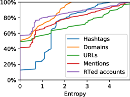
(a) DS1.

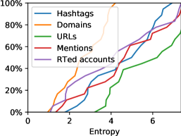
(b) DS2.

(c) RANDOM.

Figure 7: Cumulative frequency of HCCs’ entropy scores for five tweet features, comparing DS1 and DS2 with RANDOM ($\gamma$=$15$, FSA_V). Feature variation increases moving right on the x axis.

4.3.5 Multiple criteria: Bullying

Some strategies can involve a combination of actions. Behaviours that contribute to Bullying by dogpiling, for example, include joining conversations started by the target’s posts and mentioning the target repeatedly, within a confined timeframe. As DS1 included all replied to tweets, we investigated it inferring links via co-mentions and co-convs with a window size of $10$ minutes, and FSA_V with $\theta$=$0.001$, having maximised the ratio of MEW to HCC size. Of $142$ HCCs discovered, the largest had five accounts and most only had two. Only $32$ had more than ten inferred connections, but five have more than $1,000$. These heavily connected accounts, after deep analysis, were simply very active Twitter users who engaged others in conversation via mentions, which outweighed the more strict co-conv criterion of participants replying into the same conversation reply tree.

A larger window size was considered ($\gamma$=$360$) in case co-conv interactions were more prevalent. FSA_V ($\theta$=$0.01$) exposed little further evidence of co-conv (Figure 8), finding $98$ small HCCs again dominated by co-mentions, not many of which had more than one inferred connection, implying most links were incidental; FSA_V did not filter these out.

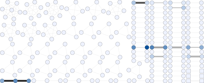
Figure 8: While searching for Bullying behaviour in DS1, these are HCCs of accounts found engaging in co-mentions (circles) and co-mentions plus co-convs, i.e., engaged in both (square vertices in bottom right) ($\gamma$=360, FSA_V, $\theta$=$0.01$). Edge thickness and darkness = inferred connections (darker = more). Vertex colour = tweets posted by that account (darker = more). Created with visone (https://visone.info).

This provides an argument for a more sophisticated approach to combining LCN edge weights for analysis, instead of Equation (1), and that FSA_V could be modified to better balance HCC size and edge weight. Furthermore, it is likely that bullying accounts will not just co-mention accounts frequently, but have low diversity in the accounts they co-mention, i.e., they repeatedly co-mention a small number of accounts. That nuance is not explored here.

4.3.6 HCC inter-relationships

Introducing vertices to represent the reasons HCC accounts are connected (e.g., who they co-mention, or conversations they join) shows how the HCCs inter-relate. Figure 9 shows the largest component after such expansion was conducted on the HCCs in Figure 8. HCC accounts (circles) share colours and the distribution of the reasons for their connection (diamonds) show which are unique to HCCs and which are shared. Heavy links between HCC accounts with few adjacent reason vertices imply these are accounts mentioned many times.

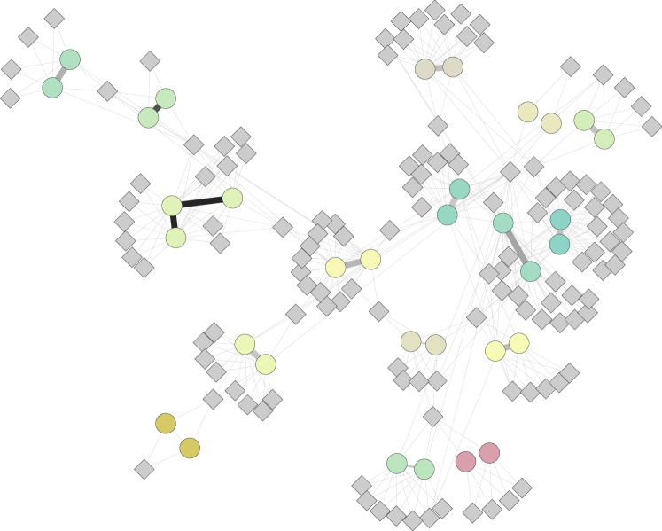
Figure 9: A graph of DS1 HCC accounts (circle vertices) connected to the accounts they mention or conversations they join (diamonds). Accounts in the same HCC share colours. Clear communities surrounding HCCs indicate who they converse with, and which conversants are co-mentioned by mulitple HCC accounts. Created with visone (https://visone.info).

4.3.7 Boosting accounts, not tweets

It is possible to Boost an account rather than just a post. Returning to DS2, we sought HCCs from accounts retweeting the same account (FSA_V, $\gamma$=$15$), and found that the hashtag use revealed further insights (Figure 10). No longer does one HCC dominate the hashtags. Instead clear themes are exhibited by different HCCs, but again, they are not the largest HCCs. The red HCC uses #blacklivesmatter-related hashtags, while the purple HCC uses pro-Republican ones (#maga and #tcot), and the green HCC is more general. Given the number of tweets these HCCs posted over 2016 (at least $16,849$), it is clear they concentrated their messaging on particular topics, some politically charged.

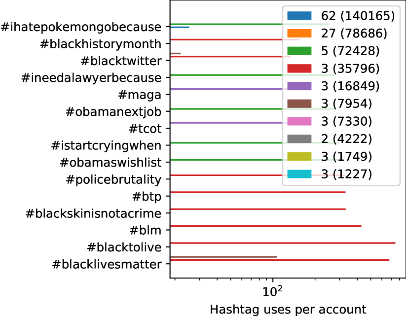
Figure 10: Most used hashtags (per account) of the most active HCCs boosting accounts (FSA_V, $\gamma$=$15$). The labels indicate member and tweet counts. Not all HCCs used a hashtag often enough to be visible.

5 Conclusion

As online influence operations grow in sophistication, our automation and campaign detection methods must also expose the accounts covertly engaging in “orchestrated activities” [26]. We have described several coordination strategies, their purpose and execution methods, and demonstrated a novel pipeline-based approach to finding sets of accounts engaging in such behaviours in two relevant datasets. Using discrete time windows, we temporally constrain potentially coordinated activities, successfully identifying groups operating over various timeframes. The analysis of HCC evolution, improvement of HCC extraction techniques and investigation of near real time processing provide opportunities for future research in this increasingly important field.

References

- [1] A. Carvin, Distant Witness: Social media, the Arab Spring and a journalism revolution. CUNY Journalism Press, 2012.
- [2] A. Bessi and E. Ferrara, “Social bots distort the 2016 U.S. Presidential election online discussion,” First Monday, vol. 21, no. 11, 2016.
- [3] E. Ferrara, “Disinformation and social bot operations in the run up to the 2017 French presidential election,” First Monday, vol. 22, no. 8, 2017.
- [4] F. B. Keller, D. Schoch, S. Stier, and J. Yang, “How to manipulate social media: Analyzing political astroturfing using ground truth data from South Korea,” in ICWSM. AAAI Press, 2017, pp. 564–567.
- [5] K. Starbird, A. Arif, and T. Wilson, “Disinformation as collaborative work: Surfacing the participatory nature of strategic information operations,” PACMHCI, vol. 3, no. CSCW, pp. 127:1–127:26, 2019.
- [6] K. Starbird and T. Wilson, “Cross-Platform Disinformation Campaigns: Lessons Learned and Next Steps,” Harvard Kennedy School Misinformation Review, jan 2020.
- [7] M.-A. Rizoiu, T. Graham, R. Zhang, Y. Zhang, R. Ackland, and L. Xie, “#DebateNight: The role and influence of socialbots on Twitter during the 1st 2016 U.S. Presidential debate,” in ICWSM. AAAI Press, 2018, pp. 300–309.
- [8] S. C. Woolley and D. R. Guilbeault, “Computational propaganda in the United States of America: Manufacturing consensus online,” Oxford, UK: Project on Computational Propaganda, Working Paper 2017.5, Jun. 2017.
- [9] K. Lee, J. Caverlee, Z. Cheng, and D. Z. Sui, “Campaign extraction from social media,” ACM TIST, vol. 5, no. 1, pp. 9:1–9:28, 2013.
- [10] O. Varol, E. Ferrara, F. Menczer, and A. Flammini, “Early detection of promoted campaigns on social media,” EPJ Data Science, vol. 6, no. 1, p. 13, 2017.
- [11] M. Alizadeh, J. N. Shapiro, C. Buntain, and J. A. Tucker, “Content-based features predict social media influence operations,” Science Advances, vol. 6, no. 30, p. eabb5824, jul 2020.
- [12] N. Vo, K. Lee, C. Cao, T. Tran, and H. Choi, “Revealing and detecting malicious retweeter groups,” in ASONAM. ACM, 2017, pp. 363–368.
- [13] S. Gupta, P. Kumaraguru, and T. Chakraborty, “Malreg: Detecting and analyzing malicious retweeter groups,” in COMAD/CODS. ACM, 2019, pp. 61–69.
- [14] S. Kumar, W. L. Hamilton, J. Leskovec, and D. Jurafsky, “Community interaction and conflict on the web,” in WWW. ACM, 2018, pp. 933–943.
- [15] G. E. Hine, J. Onaolapo, E. D. Cristofaro, N. Kourtellis, I. Leontiadis, R. Samaras, G. Stringhini, and J. Blackburn, “Kek, cucks, and God Emperor Trump: A measurement study of 4chan’s politically incorrect forum and its effects on the web,” in ICWSM. AAAI Press, 2017, pp. 92–101.
- [16] K. H. Lim, S. Jayasekara, S. Karunasekera, A. Harwood, L. Falzon, J. Dunn, and G. Burgess, “RAPID: Real-time Analytics Platform for Interactive Data Mining,” in ECML/PKDD (3), ser. Lecture Notes in Computer Science, vol. 11053. Springer, 2018, pp. 649–653.
- [17] D. Weber, “On coordinated online behaviour,” Poster presented at the Australian Social Network Analysis Conference, Nov. 2019. [Online]. Available: https://www.slideshare.net/derekweber/on-coordinated-online-behaviour
- [18] D. Pacheco, P.-M. Hui, C. Torres-Lugo, B. T. Truong, A. Flammini, and F. Menczer, “Uncovering coordinated networks on social media,” arXiv:2001.05658v1, 2020.
- [19] F. Şen, R. T. Wigand, N. Agarwal, S. T. Yuce, and R. Kasprzyk, “Focal structures analysis: Identifying influential sets of individuals in a social network,” Social Network Analysis and Mining, vol. 6, no. 1, pp. 17:1–17:22, 2016.
- [20] A. Chen, “The Agency,” The New York Times Magazine, Jun. 2015. [Online]. Available: https://www.nytimes.com/2015/06/07/magazine/the-agency.html
- [21] G. King, J. Pan, and M. E. Roberts, “How the Chinese Government Fabricates Social Media Posts for Strategic Distraction, Not Engaged Argument,” American Political Science Review, vol. 111, no. 3, p. 484–501, 2017.
- [22] E. Ferrara, O. Varol, C. Davis, F. Menczer, and A. Flammini, “The rise of social bots,” Communications of the ACM, vol. 59, no. 7, pp. 96–104, 2016.
- [23] C. Cao, J. Caverlee, K. Lee, H. Ge, and J. Chung, “Organic or organized?: Exploring URL sharing behavior,” in CIKM. ACM, 2015, pp. 513–522.
- [24] N. Chavoshi, H. Hamooni, and A. Mueen, “Temporal patterns in bot activities,” in WWW (Companion Volume). ACM, 2017, pp. 1601–1606.
- [25] F. Morstatter, Y. Shao, A. Galstyan, and S. Karunasekera, “From Alt-Right to Alt-Rechts: Twitter analysis of the 2017 German Federal Election,” in WWW (Companion Volume). ACM, 2018, pp. 621–628.
- [26] C. Grimme, D. Assenmacher, and L. Adam, “Changing perspectives: Is it sufficient to detect social bots?” in HCI (13), ser. Lecture Notes in Computer Science, vol. 10913. Springer, 2018, pp. 445–461.
- [27] P. Holme and J. Saramäki, “Temporal networks,” Physics Reports, vol. 519, no. 3, pp. 97–125, 2012.
- [28] D. Assenmacher, L. Adam, H. Trautmann, and C. Grimme, “Towards real-time and unsupervised campaign detection in social media,” in The Thirty Third International FLAIRS Conference. AAAI Publications, 2020.
- [29] A. McGregor, “Graph stream algorithms: a survey,” SIGMOD Record, vol. 43, no. 1, pp. 9–20, 2014.
- [30] M. Nasim, A. Nguyen, N. Lothian, R. Cope, and L. Mitchell, “Real-time detection of content polluters in partially observable Twitter networks,” in WWW (Companion Volume). ACM, 2018, pp. 1331–1339.
- [31] J. Burgess and A. Matamoros-Fernández, “Mapping sociocultural controversies across digital media platforms: one week of #gamergate on Twitter, YouTube, and Tumblr,” Communication Research and Practice, vol. 2, no. 1, pp. 79–96, 2016.
- [32] E. Mariconti, J. Onaolapo, S. S. Ahmad, N. Nikiforou, M. Egele, N. Nikiforakis, and G. Stringhini, “What’s in a name?: Understanding profile name reuse on Twitter,” in WWW. ACM, 2017, pp. 1161–1170.
- [33] F. Giglietto, N. Righetti, L. Rossi, and G. Marino, “It takes a village to manipulate the media: Coordinated link sharing behavior during 2018 and 2019 Italian elections,” Information, Communication & Society, pp. 1–25, mar 2020.
- [34] V. D. Blondel, J.-L. Guillaume, R. Lambiotte, and E. Lefebvre, “Fast unfolding of communities in large networks,” Journal of Statistical Mechanics: Theory and Experiment, vol. 2008, no. 10, p. P10008, 2008.
- [35] Y. Fang, X. Huang, L. Qin, Y. Zhang, W. Zhang, R. Cheng, and X. Lin, “A survey of community search over big graphs,” The VLDB Journal, vol. 29, no. 1, pp. 353–392, jul 2019.
- [36] Q. Zhao, M. A. Erdogdu, H. Y. He, A. Rajaraman, and J. Leskovec, “SEISMIC: A self-exciting point process model for predicting tweet popularity,” in KDD. ACM, 2015, pp. 1513–1522.
- [37] D. Pacheco, A. Flammini, and F. Menczer, “Unveiling coordinated groups behind white helmets disinformation,” in WWW (Companion Volume). ACM / IW3C2, 2020, pp. 611–616.
- [38] M. Damashek, “Gauging similarity with n-grams: Language-independent categorization of text,” Science, vol. 267, no. 5199, pp. 843–848, 1995.