Sampling and homology via bottlenecks

Abstract.

In this paper we present an efficient algorithm to produce a provably dense sample of a smooth compact variety. The procedure is partly based on computing bottlenecks of the variety. Using geometric information such as the bottlenecks and the local reach we also provide bounds on the density of the sample needed in order to guarantee that the homology of the variety can be recovered from the sample. An implementation of the algorithm is provided together with numerical experiments and a computational comparison to the algorithm by Dufresne et. al. [17].

1. Introduction

Sampling an object is an important problem when trying to recover information about its structure [27, 16, 17, 11, 4]. Efficiency of the sampling algorithm becomes central as many techniques tend to grow exponentially in complexity with the ambient dimension. In our setting, the objects we study are zero-sets of polynomial equations. More precisely, we study smooth, compact algebraic varieties in $\mathbb{R}^{n}$. The information we want to recover are topological invariants describing the shape of the variety, such as the homology groups. For instance, the zeroth homology group counts the number of connected components of the variety. The techniques we develop can be applied in a range of areas where the object of study is algebraic in nature, for instance kinematics [14, 28] and biochemistry [12].

Existing algorithms for sampling algebraic varieties can be divided into two categories: probabilistic methods [4, 16, 11] and provably dense sampling [17]. In Section 4 we develop a sampling technique that constructs a provably dense sample on $X$. We also provide a computational comparison to the algorithm by Dufresne et. al. [17] (see Section 4.5) showing better performance of our algorithm as the codimension increases. A public implementation of our algorithm is available at [21].

By provably dense sample we mean an $\epsilon$-sample in the sense of the following definition:

Definition.

A sample of a variety $X\subset\mathbb{R}^{n}$ is a finite subset $E\subset X$. For $\epsilon>0$ a sample $E\subset X$ is called an $\epsilon$-sample if for every $x\in X$ there is an element $e\in E$ such that $\|x-e\|<\epsilon.$ In this case we also say that $E$ is $\epsilon$-dense.

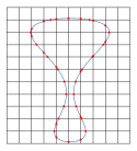
To produce an $\epsilon$-sample from $X$ we start from its defining equations. The basic idea is then to intersect the variety with a grid of linear spaces of complementary dimension. Figure LABEL:fig:planar-curve-intro shows a curve in $\mathbb{R}^{2}$ intersected with a 2-dimensional grid. The grid-size, denoted by $\delta,$ is determined by the narrowest bottleneck of the variety. A bottleneck of $X$ is a pair of distinct points $x,y\in X$ such that $(x-y)$ is normal to $X$ at both $x$ and $y$. Estimates for the number of bottlenecks and numerical algorithms to compute them have been recently studied, see [19, 15]. In Section 3 we give a system of equations defining the bottlenecks of $X$. In case $X$ has only finitely many bottlenecks, these equations can be used to find all bottlenecks, including the narrowest one. In Theorem 3.9 we provide conditions under which finiteness is achieved:

Theorem.

3.9. A generic complete intersection has only finitely many bottlenecks.

(a)

(b)

The density guarantee is achieved by introducing extra sample points given by ad hoc slicing and nearest point computations (see Section 4.2). Figure LABEL:fig:surface shows an $\epsilon$-sample of a surface in $\mathbb{R}^{4}$ with $\epsilon=0.1$.

Specifically we prove that:

Theorem.

4.6 Let $b_{2}$ be the radius of the narrowest bottleneck of $X$ and let $\epsilon>0$. If $0<\delta\sqrt{n}<\min\{\epsilon,2b_{2}\}$, then $S_{\delta}$ is an $\epsilon$-sample of $X$.

Section 5 is devoted to homology computations from a given sample. Given an $\epsilon$-sample of $X$ it is straightforward to compute the homology groups of $X$ assuming that $\epsilon$ is small enough. In [7] it is shown that the homology groups of $X$ can be recovered from the sample if $\epsilon<\tau_{X}$, where $\tau_{X}$ is the reach of $X$ (defined in Section 2). The reach and bottlenecks are geometric invariants of $X$ specific to its embedding in $\mathbb{R}^{n}$. They contribute to estimates on how dense we have to sample $X$ in order to be able to recover its shape. In this paper we show that the density of the sample needed to compute the zeroth and first homology groups of $X$ is controlled by the radii of the generalized bottlenecks (see Section 3). The radius of the narrowest generalized bottleneck is equivalent to the weak feature size (wfs) introduced in [10]. One of the main contributions of this paper is the following result:

Theorem.

5.4. Let $\epsilon<wfs(X)$ and let $i\in\{0,1\}$. Let $E$ be an $\epsilon$-dense sample of $X$ and let $S$ be the modified Vietoris-Rips complex constructed from $E$ as in Section 5.1. Then,

$$H_{i}(S)\cong H_{i}(X)$$

Computing the bottlenecks is in general much easier than computing the reach. Therefore, in cases where the radius of the narrowest bottleneck is equal to the wfs we obtain sparser samples and considerable computational improvements for varieties with high curvature. We believe it to be true that the narrowest bottleneck equals the wfs for generic varieties, but this needs further investigation. In Example 5.5 we provide a comparison with existing algorithms in [7].

For the higher homology groups we provide the following result saying that we can bound the reach from below using estimates of the local reach $\tau_{X}(p)$ (see Section 2) for sample points $p\in X$. The homology of $X$ can then be computed from the C̆ech complex, $C(E,\epsilon)$, given by the nerve of the union of all closed $\epsilon$-balls $\bar{B}_{e}(\epsilon)$ for each $e\in E$.

Theorem.

5.6. If $E\subset X$, $\epsilon>0$, $E$ is an $(\epsilon/2)$-sample and $\epsilon<\frac{4}{5}\tau_{X}(e)$ for all $e\in E$, then $X$ is a deformation retract of $C(E,\epsilon)$. In particular, $X$ and $C(E,\epsilon)$ have the same homology groups.

As estimating the reach of a manifold is computationally a very challenging problem, our approach provides an important simplification. The estimate is based on a finite process i.e. computing the local reach at finetly many sample points. It is an interesting problem to further investigate the implications of local approaches like this for the computational complexity of homology groups. Roughly speaking we expect the size of a sample of the ambient space $\mathbb{R}^{n}$ to be exponential in $n$ but a sample of $X$ to be exponential in $\operatorname{dim}(X)$.

Acknowledgements.

The authors would like to thank Parker Edwards for interesting discussions and Sascha Timme for helping with the implementation, which uses the HomotopyContinuation.jl [6] software package. Mathematica [25] and Matplotlib [24] were used for creating images. The third author was supported by the Thematic Einstein Semester ”Varieties, Polyhedra, Computation” by the Berlin Einstein Foundation. All three authors acknowledge generous support by Vetenstapsrådet grants [NT:2014-4763], [NT:2018-03688].

2. Geometrical background

Let $X\subseteq\mathbb{C}^{n}$ be a smooth subvariety and let $q\in\mathbb{R}^{n}$. For $x\in X$, $N_{x}X\subseteq\mathbb{C}^{n}$ denotes the embedded normal space to $X$ at $x$. Consider the set of critical points with respect to the squared Euclidean distance function from $X$ to $q$:

$$I(X,q)=\{x\in X:q\in N_{x}X\}.$$

We call $I(X,q)$ the normal locus of $X$ with respect to $q$. Consider the real part $X_{\mathbb{R}}\subset\mathbb{R}^{n}$ of $X$. We will use the notation $I(X_{\mathbb{R}},q)$ to denote the real points in $I(X,q)$.

The degree of $I(X,q)$ for generic $q\in\mathbb{C}^{n}$ is called the Euclidean Distance Degree (EDD) of $X$. If $X$ is a complete intersection defined by $f_{1},\dots,f_{c}\in\mathbb{C}[x_{1},\dots,x_{n}]$, then $I(X,q)$ may be computed via the following system of equations:

(1) $$f_{1}(x)=\ldots=f_{c}(x)=0$$

(2) $$x-q=\sum_{i=1}^{c}\lambda_{i}\nabla f_{i}(x),$$

where $\lambda_{i}$ are auxiliary variables and $\nabla f_{i}$ denotes the gradient of $f_{i}$. To compute $I(X,q)$, in case it is finite, one can for instance use numerical homotopy methods [2, 30, 3]. Note that the system (1) is linear in $\lambda_{i}$ and so it is advantageous to use a multihomogeneous homotopy to solve it.

Consider a smooth variety $X_{\mathbb{C}}\subset\mathbb{C}^{n}$ and its real part $X\subseteq\mathbb{R}^{n}$ and let $q\in\mathbb{R}^{n}\setminus X$. One reason that $I(X,q)$ is interesting is that it contains at least one point on every connected component of $X$, namely the point closest to $q$. This will be useful in the sampling algorithm presented in Section 4.

Below we will need to find a bounding box of a non-empty compact smooth variety $X\subset\mathbb{R}^{n}$. One way to do this is to compute the normal locus $I(X,q)=\{x\in X:q\in N_{x}{X}\}$ with respect to a random point $q\in\mathbb{R}^{n}$. From $I(X,q)$ we get enough information to find a bounding box or a bounding ball of $X$, that is a box or ball that contains $X$. Let $\bar{B}_{q}(r)\subset\mathbb{R}^{n}$ be the closed ball of radius $r$ centered at $q\in\mathbb{R}^{n}$. Since $X$ is compact, for any $q\in\mathbb{R}^{n}$ there is a point $x\in I(X,q)$ that maximizes the distance from $q$ to points of $X$. Hence $X\subset\bar{B}_{q}(||x-q||)$. The solid hypercube with side length $2||x-q||$ centered at $q$ is then a bounding box for $X$.

As above let $X\subset\mathbb{R}^{n}$ be a compact smooth variety. A very important invariant of the embedding $X\subset\mathbb{R}^{n}$ of a variety is the reach of $X$. For $p\in\mathbb{R}^{n}$, let $\pi_{X}(p)$ denote the set of points $x\in X$ such that $||x-p||=\min_{x^{\prime}\in X}||x^{\prime}-p||$. Also, for $r\geq 0$ let $X_{r}$ denote the tubular neighborhood of $X$ of radius $r$, that is the set of points $x\in\mathbb{R}^{n}$ at distance less than $r$ from $X$. Then the reach $\tau_{X}$ of $X$ may be defined as $\sup\{r\geq 0:|\pi_{X}(p)|=1\textrm{ for all }p\in X_{r}\}$. For a point $q\in X$ we have a local notion called the local reach, or the local feature size, which is defined as $\tau_{X}(q)=\sup\{r\geq 0:|\pi_{X}(p)|=1\textrm{ for all }p\in B_{q}(r)\}$ where $B_{q}(r)=\{p\in\mathbb{R}^{n}:||p-q||<r\}$. Then $\tau_{X}=\inf_{q\in X}\tau_{X}(q)$. Since $X$ is compact the reach is positive and if we in addition assume that $\operatorname{dim}(X)>0$, $X$ is not convex and therefore the reach of $X$ is finite. The reach can be computed as a minimum of two quantities [1], one of which derives from local considerations in terms of the curvature of $X$ and the other one is a global quantity arising from the bottlenecks of $X$. More precisely, the global quantity is the radius of the narrowest bottleneck of $X$. The local quantity, which we call $\rho$, is the minimal radius of curvature on $X$, where the radius of curvature at a point $x\in X$ is the reciprocal of the maximal curvature of a geodesic passing through $x$. The global quantity is $\frac{1}{2}\inf\{||x-y||:(x,y)\in X\times X,\,x\neq y,\,y\in N_{x}{X},\,x\in N_{y}{X}\}$ where $N_{p}X\subset\mathbb{R}^{n}$ denotes the normal space of $X$ at a point $p\in X$.

Let $\Delta_{X}=\{p\in\mathbb{R}^{n}:|\pi_{X}(p)|>1\}$ and define the medial axis $M_{X}$ as the closure of $\Delta_{X}$. Let $U_{X}=\mathbb{R}^{n}\setminus M_{X}$ and note that the projection $\pi_{X}$ is a well defined map $\pi_{X}:U_{X}\rightarrow X$ which maps a point $p$ to the unique closest point of $X$. Also, the local reach $\tau_{X}(q)$ is the distance from $q\in X$ to the medial axis and the reach $\tau_{X}$ is the distance from $X$ to the medial axis.

3. Bottlenecks and Reach

3.1. Weak feature size

We will first define a generalized version of bottlenecks inspired by the construction in [10]. Let $X\subset\mathbb{C}^{n}$ be a smooth variety. For a set of points $x_{1},\dots,x_{k}\in X$ to define a bottleneck we first require there to be a point $y\in\mathbb{C}^{n}$ such that the Euclidean distance from $y$ to $x_{i}$ is the same for each $0\leq i\leq k$ and that $y$ is in the normal space $N_{X}(x_{i})$ for each $0\leq i\leq k$. Moreover, we would like $y$ to be critical in some sense. It turns out that a good notion of critical is that $y$ is in the convex hull of $x_{1},\dots,x_{k}$. This means that there exists real non-negative numbers $a_{1},\dots,a_{k}$ such that $\sum_{i=1}^{k}a_{i}=1$ and $y=\sum_{i=1}^{k}a_{i}x_{i}$. We refer to [10] for more details. To formalize this idea we make the following definitions.

Definition 3.1.

Let $C\coloneqq\{(y,r)\in\mathbb{C}^{n}\times\mathbb{C}\mid||x_{i}-y||^{2}-r=0,\text{ for $1\leq i\leq k$}\}$ and denote the closure of the projection $C\to\mathbb{C}^{n}$ by $\rho(x_{1},\dots,x_{k})$. Then $\rho(x_{1},\dots,x_{k})$ is the set of centers of all $(n-1)$-spheres passing through the points $x_{1},\dots,x_{k}$. Next, let $Conv(x_{1},\dots,x_{k})$ denote the convex hull of the points $x_{1},\dots,x_{k}$. Define the $k$th bottleneck locus to be the following set:

$$B_{k}\coloneqq\{(x_{1},\dots,x_{k})\in\mathbb{C}^{n\times k}\setminus\Delta\mid\cap_{i=1}^{k}N_{X}(x_{i})\cap\rho(x_{1},\dots,x_{k})\cap Conv(x_{1},\dots,x_{k})\neq\emptyset\}$$

where $\Delta\coloneqq\{(x_{1},\dots,x_{k})\mid x_{i}=x_{j}\text{ for some $i,j$}\}\subset\mathbb{C}^{n\times k}$.

Note that $B_{1}=X$ and $B_{2}$ is what is usually defined as the bottleneck locus. In the case $k=2$ the conditions in the above definition simplify to algebraic conditions which means that $B_{2}$ is an algebraic variety in $\mathbb{C}^{2n}$. For $k>2$ the set $B_{k}$ is not algebraic but if we restrict $B_{k}$ to only allow real tuples $(x_{1},\dots,x_{k})\in\mathbb{R}^{n\times k}$ it is a semi-algebraic set.

Remark 3.2.

In general, $B_{k}$ is empty for $k>EDD(X)$ since there is no point in $\mathbb{C}^{n}$ which is in the normal space of more than $EDD(X)$ number of points on $X$. The only case for which $B_{k}$ is not empty for $k>EDD(X)$ is if there is a point $q\in\mathbb{C}^{n}$ which is in the normal space of infinitely many points on $X$. This is the case for instance if $X$ contains a component which is an $m$-sphere for some $m\geq 1$. In this case $B_{k}$ is infinite for all $k\in\mathbb{N}$. The sets $B_{k}$ for $k>EDD(X)$ don’t contribute to new information for our purposes in this case and we will therefore not consider them.

By restricting the sets $B_{k}$ to only allow tuples in $\mathbb{R}^{n}$ we can define a notion of narrowest bottleneck. Let $B^{\mathbb{R}}_{k}$ denote this restriction.

Definition 3.3.

Let $\ell_{k}\colon B^{\mathbb{R}}_{k}\to\mathbb{R}$ be the function that takes $(x_{1},\dots,x_{k})$ to the radius of the smallest $(n-1)$-sphere satisfying the condition in Definition 3.1. Define $b_{k}$ to be the minimal value (or infimum in case $B^{\mathbb{R}}_{k}$ is not finite) of the image of $\ell_{k}$, called the radius of the narrowest bottleneck of degree $k$. We now define the weak feature size as the following quantity:

$$wfs(X)\coloneqq\underset{2\leq k\leq EDD(X)}{min}b_{k}$$

For the remainder of this paper we will refer to elements of $B_{2}$ as the bottlenecks of $X$ and elements of $B_{k}$ for $k>2$ as generalized bottlenecks of degree $k$. The narrowest bottleneck of $X$ thus refers to the narrowest bottleneck of degree 2 of $X$.

Computing the generalized bottlenecks of $X$ is in general much harder than computing $b_{2}$. It is therefore interesting to understand in which cases the equality $wfs(X)=b_{2}$ holds.

Example 3.4.

Let $f_{1}(x,y)=3x^{2}y-y^{3}+2(x^{2}+y^{2})(x^{2}+y^{2}-1)$ and $f_{2}(x,y)=10x^{2}y^{3}-5x^{4}y-y^{5}+5(x^{2}+y^{2})^{2}(x^{2}+y^{2}-1)$. The curves $\{f_{1}=0\}$ and $\{f_{2}=0\}$ are two examples of varieties in $\mathbb{R}^{2}$ for which the weak feature size, $wfs(X)$, is smaller than the narrowest bottleneck $b_{2}$.

(c) third

(d) fourth

Figure 1. Two examples of when the weak feature size is smaller than the narrowest bottleneck of a variety.

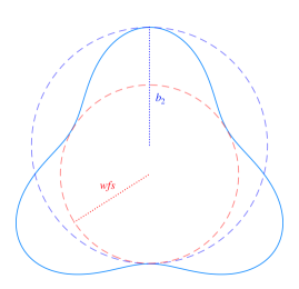
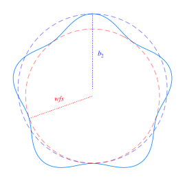
The varieties in Figure 1 illustrate two examples in $\mathbb{R}^{2}$ of when the equality $wfs(X)=b_{2}$ fails. Both of these examples are oscillations of a circle in the sense that they can be described in the polar plane as $r=1+f(\cos(n\theta))$ for some function $f\colon\mathbb{R}\to\mathbb{R}$ and $n\in\mathbb{Z}$. Note that the curve segments between points of the generalized bottlenecks in Figure 1 cannot bend too much, since then we would have a degree 2 bottleneck of smaller radius. It seems probable in $\mathbb{R}^{2}$ that $wfs(X)<b_{2}$ only if $X$ contains a component which is an oscillation of a circle, although this requires further investigation. We therefore make the conjecture that the equality $wfs(X)=b_{2}$ holds in general.

3.2. Computing bottlenecks

Let $X\subseteq\mathbb{C}^{n}$ be a smooth variety defined by a system of equations $F=(f_{1},\dots,f_{r})\subset\mathbb{C}[x_{1},\dots,x_{n}]$. The bottlenecks of $X$ consists of pairs of distinct points $x,y\in X$ such that $(x-y)\perp T_{x}X$ and $(x-y)\perp T_{y}X$. Here, $v\perp w$ means that $\sum_{i=1}^{n}v_{i}w_{i}=0$ where $v=(v_{1},\dots,v_{n})\in\mathbb{C}^{n}$ and $w=(w_{1},\dots,w_{n})\in\mathbb{C}^{n}$. Let $J_{F}$ denote the Jacobian matrix of $F$, let $c=\operatorname{codim}(X)$ and assume that $c<n$. Expressed in terms of defining equations, $(x,y)$ with $x\neq y$ is a bottleneck precisely when the matrices

$$\begin{pmatrix}x-y\\ J_{F}(x)\end{pmatrix},\quad\begin{pmatrix}x-y\\ J_{F}(y)\end{pmatrix}$$

both have rank $\leq c$. The bottlenecks of $X$ are thus part of the zero locus $Z\subseteq X\times X$ of the system given by the $(c+1)\times(c+1)$-minors of these matrices together with the defining equations $F(x)$ and $F(y)$. Then $Z\setminus\Delta$ describes the bottleneck locus $B_{2}$, where $\Delta\subset X\times X$ is the diagonal.

An efficient method to compute all isolated bottlenecks of a smooth algebraic variety in general position is presented in [19]. The method makes use of numerical homotopy methods [30, 3]. Suppose that $X\subset\mathbb{R}^{n}$ is smooth and compact. As we saw in Section 2, the radius of the narrowest bottleneck is intimately connected to the reach of $X$. Even though the bottleneck locus is expected to be finite, it might not be and in this case we would be required to solve an optimization problem to find the narrowest bottleneck. The case of finitely many bottlenecks is simpler since then computing all the bottlenecks suffices. For these reasons (among others) it is useful to know when the bottleneck locus is finite. In this section we provide a first step in this direction by proving that general complete intersections have only finitely many bottlenecks. Regarding the number of bottlenecks for general enough algebraic varieties, a formula for low dimensional varieties is given in [15].

Let $(d_{1},\dots,d_{c})\in\mathbb{N}^{c}$ with $d_{i}\geq 1$ and let $P_{i}=\mathbb{P}^{N_{i}}$ where $N_{i}={d_{i}+n\choose d_{i}}-1$ be the parameter space of hypersurfaces in $\mathbb{C}^{n}$ of degree at most $d_{i}$. Complete intersections in $\mathbb{C}^{n}$ of codimension $c$ and degree type $(d_{1},\dots,d_{c})$ are parameterized by an open subset $U\subset\prod_{i=1}^{c}P_{i}$ and we write $X_{u}\subseteq\mathbb{C}^{n}$ for the complete intersection corresponding to $u\in U$. Let $V=\mathbb{C}^{n}\times\mathbb{C}^{n}\setminus\Delta$, where $\Delta$ is the diagonal.

If $c=n$ the complete intersection itself is finite, hence we assume that $c<n$. We may also assume that none of the equations are linear, that is $d_{i}\geq 2$ for all $i$. For a generic hyperplane $H\subset\mathbb{C}^{n}$ there is a complex orthogonal linear map which takes $H$ to the hyperplane $\{x_{1}=0\}$ and such a linear map preserves bottlenecks. Moreover, a smooth variety $X\subseteq\mathbb{C}^{n-1}$ with $\mathbb{C}^{n-1}=\{x_{1}=0\}\subset\mathbb{C}^{n}$ has the same bottlenecks when seen as a subvariety of $\mathbb{C}^{n}$. By induction on the number of linear equations we may assume that $d_{i}\geq 2$ for all $i$.

Definition 3.5.

Let the bottleneck correspondence denote the following set:

$$U\times V\supseteq\mathcal{B}\coloneqq\{(u,x,y):x,y\in X_{u},(x-y)\perp T_{x}X_{u},(x-y)\perp T_{y}X_{u}\}.$$

In order to show that a general complete intersection has finite bottleneck locus we need to show that the generic fiber of the projection $\eta:\mathcal{B}\to U$ is finite. We do this by first studying the dimension of the fibers of the projection $\pi:\mathcal{B}\to V$.

Consider invertible affine transformations $g:\mathbb{C}^{n}\to\mathbb{C}^{n}$ of the form $gx=R(sx+t)$ where $t\in\mathbb{C}^{n}$ is a translation, $s\in\mathbb{C}^{*}$ is a scaling and $R\in O(n)$ is a complex orthogonal map. Let $G$ denote the subgroup of all such transformations of the group of invertible affine transformations of $\mathbb{C}^{n}$. Then $G$ acts on $\mathbb{C}^{n}$ and $G$ acts on $U$ by pre-composition of the defining equations with $g^{-1}$ for $g\in G$. Moreover, $G$ acts on $\mathcal{B}$ via $g(u,x,y)=(gu,gx,gy)$ and on $V$.

Lemma 3.6.

Let $e_{1},\dots,e_{n}$ denote the standard basis in $\mathbb{C}^{n}$. The action of $G$ on $V$ has two orbits generated by the pairs $(e_{1},0)$ and $(e_{1}+ie_{2},0)$.

Proof.

The group $O(n)$ acts transitively on the sphere $S^{n-1}=\{x\in\mathbb{C}^{n}:\sum_{i}x_{i}^{2}=1\}$. Therefore the equation $Mx=se_{1}$, where $M\in O(n)$ and $s\in\mathbb{C}^{*}$, has a solution whenever $x^{T}x\neq 0$. Consequently, for any $(a,b)\in V$ with $(a-b)^{T}(a-b)\neq 0$, there exists a $g\in G$ such that $g(a,b)=(e_{1},0)$. Let $Q\coloneqq\{(a,b)\in V\mid(a-b)^{T}(a-b)=0\}$. It remains to show that for any $(a,b)\in Q$, there is a $g\in G$ such that $g(a,b)=(e_{1}+ie_{2},0)$. This means that there is an $M\in O(n)$ and $s\in\mathbb{C}^{*}$ such that

$$sM(a-b)=e_{1}+ie_{2}\Leftrightarrow s(a-b)=M^{-1}(e_{1}+ie_{2})=m_{1}+im_{2}$$

where $m_{1},m_{2}$ are the first two columns of $M^{-1}$. Note that $(m_{1}+im_{2})^{T}(m_{1}+im_{2})=0$ since $m_{1}^{T}m_{2}=0$ and $m_{1}^{T}m_{1}=m_{2}^{T}m_{2}=1$. It is straightforward to see that any non-zero vector $x\in\mathbb{C}^{n}$ such that $x^{T}x=0$ can be written as a sum $\frac{1}{s}(m_{1}+im_{2})$ of two orthonormal vectors $m_{1},m_{2}$ and a scalar $s$. Namely, for any non-zero entry $x_{i}$ of $x$, we have that $x=x_{i}(e_{i}+\frac{1}{x_{i}}(x-x_{i}e_{i}))$. ∎

Note that the projection $\pi:\mathcal{B}\to V$ is equivariant under the action of $G$. This means that $\operatorname{dim}(\pi^{-1}(x,y))$ is the same for all $(x,y)\in V$ within the same orbit. We will first compute $\operatorname{dim}(\pi^{-1}(x,y))$ for elements in the orbit generated by $(e_{1},0)$.

Lemma 3.7.

The codimension of $\pi^{-1}(e_{1},0)$ as a subvariety of $U$ is $2n$.

Proof.

For $u\in U$ let $F_{u}$ denote the corresponding system of equations and consider the $(c+1)\times n$-matrices

$$\begin{pmatrix}e_{1}\\ J_{F_{u}}(e_{1})\end{pmatrix}=\begin{pmatrix}1&0&\dots&0\\ &&J_{F_{u}}(e_{1})&\end{pmatrix},\quad\begin{pmatrix}e_{1}\\ J_{F_{u}}(0)\end{pmatrix}=\begin{pmatrix}1&0&\dots&0\\ &&J_{F_{u}}(0)&\end{pmatrix}.$$

The condition defining $\pi^{-1}(e_{1},0)$ is that these matrices drop rank and that $F_{u}(e_{1})=0$ and $F_{u}(0)=0$. The condition that the above matrices drop in rank is equivalent to the condition that the $c\times(n-1)$-matrices ${J}_{F^{\prime}_{u}}(e_{1})$ and ${J}_{F^{\prime}_{u}}(0)$ drop rank, where ${J}_{F^{\prime}_{u}}$ is $J_{F_{u}}$ with the first column removed.

We shall see that the entries of $F_{u}(e_{1})$, $F_{u}(0)$, ${J}_{F^{\prime}_{u}}(e_{1})$ and ${J}_{F^{\prime}_{u}}(0)$ are all independent as homogeneous linear forms in $u\in U$. Independence across different equations is clear since these involve disjoint groups of variables coming from different spaces $P_{i}$. It is therefore enough to consider the case $c=1$ of one polynomial $f_{u}\in\mathbb{C}[x_{1},\dots,x_{n}]$. Moreover, it suffices to assume that $d_{1}=2$. Namely, if the there is a linear relation between the forms for some $d_{1}>2$, the same linear relation holds between the forms in the case $d_{1}=2$ (a set of dependent vectors in a vector space remain dependent after projection to a lower dimensional space).

Suppose $f_{u}\in\mathbb{C}[x_{1},\dots,x_{n}]$ is a generic quadric and let $\nabla f^{\prime}_{u}$ denote $\nabla f_{u}$ with the first entry removed. We will show that $f(e_{1})$, $f(0)$ and the entries of $\nabla f_{u}^{\prime}(e_{1})$ and $\nabla f_{u}^{\prime}(0)$ are all independent linear forms. Let

(3) $$f_{u}(x):=\sum_{1\leq i\leq j\leq n}u_{ij}x_{i}x_{j}+\sum_{i=1}^{n}u_{0i}x_{i}+u_{00}.$$

Then by inspection we note that the following linear forms are all linearly independent:

$$f(e_{1}) =u_{11}+u_{01}+u_{00}$$

$$f(0) =u_{00}$$

$$\nabla f_{u}^{\prime}(e_{1}) =\begin{bmatrix}u_{12}+u_{02}&u_{13}+u_{03}&\dots&u_{1n}+u_{0n}\end{bmatrix}$$

$$\nabla f_{u}^{\prime}(0) =\begin{bmatrix}u_{02}&u_{03}&\dots&u_{0n}\end{bmatrix}$$

To compute $\operatorname{dim}(\pi^{-1}(e_{1},0))$ we may now apply standard results on the dimensions of linear determinantal varieties. We can express $\pi^{-1}(e_{1},0)$ as a proper intersection of three varieties: two determinantal varieties given by the rank conditions on ${J}_{f^{\prime}_{u}}(e_{1})$ and ${J}_{f^{\prime}_{u}}(0)$ and a linear space defined by the $2c$ linear forms $f_{u}(e_{1}),f_{u}(0)$. The determinantal varieties both have codimension $n-c$ as subvarieties of $U$ by [22] Proposition 12.2. It follows that $\pi^{-1}(e_{1},0)$ has codimension $2n$ as a subvariety of $U$. ∎

It remains to compute $\operatorname{dim}(\pi^{-1}(x,y))$ for the orbit generated by $(e_{1}+ie_{2},0)$.

Lemma 3.8.

The codimension of $\pi^{-1}(e_{1}+ie_{2},0)$ as a subvariety of $U$ is $2n$ except in the special case when $c=1$ and deg$(X_{u})=2$ in which case it is $2n-1$.

Proof.

Similar to the proof of Lemma 3.7 we consider the following $(c+1)\times n$-matrices:

(4) $$\begin{pmatrix}e_{1}+ie_{2}\\ J_{F_{u}}(e_{1}+ie_{2})\end{pmatrix}=\begin{pmatrix}1&i&\dots&0\\ &&J_{F_{u}}(e_{1}+ie_{2})&\end{pmatrix},\quad\begin{pmatrix}e_{1}+ie_{2}\\ J_{F_{u}}(0)\end{pmatrix}=\begin{pmatrix}1&i&\dots&0\\ &&J_{F_{u}}(0)&\end{pmatrix},$$

and again, the condition defining $\pi^{-1}(e_{1}+ie_{2},0)$ is that these matrices drop in rank and that $F_{u}(e_{1}+ie_{2})=0$ and $F_{u}(0)=0$. We may now perform the column operation where we subtract $i$ times the first column from the second column. Let $J_{F^{\prime\prime}_{u}}$ denote the result when this operation is performed on $J_{F_{u}}$ and the first column removed. The condition defining $\pi^{-1}(e_{1}+ie_{2},0)$ can now be expressed as $J_{F^{\prime\prime}_{u}}(e_{1}+ie_{2})$ and $J_{F^{\prime\prime}_{u}}(0)$ dropping rank together with $F_{u}(e_{1}+ie_{2})=0$ and $F_{u}(0)=0$.

Consider first the case $c=1$. In this case the equations defining $\pi^{-1}(e_{1}+ie_{2},0)$ are linear and we need to determine the rank of this linear system. Let $f_{u}\in\mathbb{C}[x_{1},\dots,x_{n}]$ be the polynomial defining $X_{u}$. We assume that $f_{u}$ is a general polynomial of degree three in $\mathbb{C}[x_{1},\dots,x_{n}]$. We will see that this describes the general case and that we get a special case when deg$(f_{u})=2$. The polynomial is represented as follows:

(5) $$f_{u}(x):=\sum_{1\leq i\leq j\leq k\leq n}u_{ijk}x_{i}x_{j}x_{k}+\sum_{1\leq i\leq j\leq n}u_{0ij}x_{i}x_{j}+\sum_{i=1}^{n}u_{00i}x_{i}+u_{000}.$$

$$f_{u}(e_{1}+ie_{2}) =u_{111}+iu_{112}-u_{122}-iu_{222}+u_{011}+iu_{012}-u_{022}+u_{001}+iu_{002}+u_{000}$$

$$f_{u}(0) =u_{000}$$

$$\nabla f_{u}^{\prime\prime}(e_{1}+ie_{2}) =[u_{112}+2iu_{122}-3u_{222}+u_{12}+2iu_{22}+u_{02}-i(3u_{111}+2iu_{112}-u_{122}+2u_{11}+$$

$$\ \ \ \ +iu_{12}+u_{01})\ \ \ \ u_{113}+iu_{123}-u_{223}+u_{13}+iu_{23}+u_{03}\ \ \ \ \dots\ \ \ \$$

$$\ \ \ \ \ u_{11n}+iu_{12n}-u_{22n}+u_{1n}+iu_{2n}+u_{0n}]$$

$$\nabla f_{u}^{\prime\prime}(0) =\begin{bmatrix}u_{02}-iu_{01}&u_{03}&\dots&u_{0n}\end{bmatrix}$$

The principal minors of $\nabla f_{u}^{\prime\prime}(e_{1}+ie_{2})$ and $\nabla f_{u}^{\prime\prime}(0)$ are systems of linear equations. Consequently, the system of equations determining $\pi^{-1}(e_{1}+ie_{2},0)$ is the zero set of the above linear forms. It is easily verified that all the above linear forms are linearly independent, which means that the linear system determining $\pi^{-1}(e_{1}+ie_{2},0)$ has full rank. Since there are $2n$ linear forms this means that the rank of the system is $2n$ and thus the codimension of $\pi^{-1}(e_{1}+ie_{2},0)$ as a subvariety in $U$ is $2n$. By an analogous argument as in Lemma 3.7 it then follows that this result holds for any general polynomial of degree $\geq 3$ in $\mathbb{C}[x_{1},\dots,x_{n}]$.

When $f_{u}$ has degree two we get a special case. The system describing $\pi^{-1}(e_{1}+ie_{2},0)$ is now the above system where we delete all coefficients corresponding to degree three terms. We then note that there is a linear dependence between the linear forms $f_{u}(e_{1}+ie_{2})$, $f_{u}(0)$ and the first linear forms of the vectors $\nabla f_{u}^{\prime\prime}(e_{1}+ie_{2})$ and $\nabla f_{u}^{\prime\prime}(0)$. This dependence is described by the following relation:

$$2f_{u}(e_{1}+ie_{2})-2f_{u}(0)-\big{[}u_{12}+2iu_{22}+u_{02}-i(2u_{11}+iu_{12}+u_{01})\big{]}+\big{[}u_{02}-iu_{01}\big{]}=0$$

This is the only relation between the above linear forms, let $\ell$ denote this linear relation. Hence the system of equations defining $\pi^{-1}(e_{1}+ie_{2},0)$ is a linear system of rank $2n-1$. It follows that the codimension of $\pi^{-1}(e_{1}+ie_{2},0)$ as a subvariety in $U$ is $2n-1$.

Consider now the case $c>1$ and $d_{1}=\dots=d_{c}=2$. First note that the two determinantal varieties cut out by the principal minors of $J_{F^{\prime\prime}_{u}}(e_{1}+ie_{2})$ and $J_{F^{\prime\prime}_{u}}(0)$ consist of independent linear forms and their intersection thus has codimension $2n-2c$. Note that since they each consist of disjoint variable groups it follows that their intersection is in fact a product. Each of the two determinantal varieties are by [26] irreducible and reduced and the defining equations are homogeneous of degree $c$. Now let $u=(u_{1},\dots,u_{c})$ denote the coefficients of the polynomials determining $X_{u}$. By the above results, we have two linear equations, $f_{u_{j}}(e_{1}+ie_{2})=0$ and $f_{u_{j}}(0)=0$, for each $1\leq j\leq c$ yielding $2c$ linear equations which are all linearly independent. Let $\ell_{u_{i}}$ denote the linear relation in the $c=1$ case corresponding to the $i$th defining equation of $X_{u}$. Note that since the determinantal varieties have homogeneous defining equations of degree $c$, there is no polynomial of degree $\leq c$ contained in these ideals. Thus no product $\prod_{i\in J\subset\{1,\dots,c\}}\ell_{u_{i}}$ is contained in the ideals if $|J|<c$. It is then a question if $\prod_{i\in\{1,\dots,c\}}\ell_{u_{i}}$ is in either of the determinantal ideals. But this cannot be since it would correspond to the product of the elements in one column of $J_{F^{\prime\prime}_{u}}(e_{1}+ie_{2})$ or $J_{F^{\prime\prime}_{u}}(0)$ to be in the corresponding determinantal ideal. This cannot happen since the linear forms of each matrix are linearly independent. It follows that the intersection of the determinantal varieties and the $2c$ linear forms is transverse and that the codimension of the intersection is $2n$ in $U$. The codimension of the analogous intersection when $d_{i}\geq 2$ for $1\leq i\leq c$ when $c>1$ is also $2n$ in $U$. Thus we conclude that for $c>1$, the codimension of $\pi^{-1}(e_{1}+ie_{2},0)$ as a subvariety in $U$ is $2n$. ∎

We are now ready to state the following:

Theorem 3.9.

A generic complete intersection has only finitely many bottlenecks.

Proof.

We will show that $\operatorname{dim}(\mathcal{B})=\operatorname{dim}(U)$. It follows that the general fiber of the projection $\eta:\mathcal{B}\to U$ is finite.

By Lemma 3.7 and 3.8, $\pi:\mathcal{B}\to V$ is onto and the general fiber has dimension $\operatorname{dim}(U)-2n$. Since $\operatorname{dim}(V)=2n$, it follows that $\mathcal{B}$ has an irreducible component of dimension $\operatorname{dim}(U)$. Now let $\mathcal{B}^{\prime}\subseteq\mathcal{B}$ be an irreducible component. Suppose first that $\pi(\mathcal{B}^{\prime})$ is not contained in $Q=\{(x,y)\in V\mid(x-y)^{T}(x-y)=0\}$. Then $\operatorname{dim}(\mathcal{B}^{\prime}\cap\pi^{-1}(x,y))\leq\operatorname{dim}(U)-2n$ for generic $(x,y)\in\pi(\mathcal{B}^{\prime})$ by Lemma 3.7. Hence $\operatorname{dim}(\mathcal{B}^{\prime})\leq\operatorname{dim}(U)$. Now assume that $\pi(\mathcal{B}^{\prime})\subseteq Q$. Then $\operatorname{dim}(\mathcal{B}^{\prime}\cap\pi^{-1}(x,y))\leq\operatorname{dim}(U)-2n+1$ for generic $(x,y)\in\pi(\mathcal{B}^{\prime})$ by Lemma 3.8. But $\operatorname{dim}(\pi(\mathcal{B}^{\prime}))\leq 2n-1$ in this case and hence $\operatorname{dim}(\mathcal{B}^{\prime})\leq\operatorname{dim}(U)$. ∎

3.3. Locally estimating the reach

In this section we briefly explain how the reach of a smooth variety $X\subset\mathbb{R}^{n}$ can be estimated from below by sampling the variety and estimating the local reach. We will assume that $X$ is a subvariety of the unit sphere $S^{n-1}\subset\mathbb{R}^{n}$ defined by an ideal generated by homogeneous polynomials $F=(f_{1},\dots,f_{q})$ of degrees $d_{1},\dots,d_{q}$ with $q\leq n$.

The local reach is estimated using a result of [13, 7] together with a result from Schub Smale theory. The first result bounds the local reach at a point $x\in X$ in terms of the $\gamma$-number of the system $F$ at $x$ and the second result bounds the $\gamma$-number in terms of the condition number of $F$ at $x$. To set this up we will restate some notation from [7]. Consider a homogeneous polynomial $h=\sum_{|a|=d}h_{a}x^{a}$ where $(a_{1},\dots,a_{n})$ is a multi index, $|a|=a_{1}+\dots+a_{n}$, $d$ is the degree of $h$, $h_{a}$ its coefficients and $x^{a}=x_{1}^{a_{1}}\dots x_{n}^{a_{n}}$. The Weil norm $||h||_{w}$ of $h$ is defined by $||h||_{w}^{2}=\sum_{|a|=d}h_{a}^{2}\binom{d}{a}^{-1}$ where $\binom{d}{a}=\frac{d!}{a_{1}!\cdots a_{n}!}$ are multinomial coefficients. The norm of the system $F=(f_{1},\dots,f_{q})$ is defined by $||F||^{2}=\sum_{i=1}^{q}||f_{i}||_{w}^{2}$. Let $X$ be the zero-set of $F$ and let let $DF$ be the Jacobian matrix of $F$. For $x\in X$ consider the pseudo-inverse $DF(x)^{\dagger}=DF(x)^{T}(DF(x)DF(x)^{T})^{-1}$ of $DF(x)$. Also, let $\Delta$ denote the diagonal matrix with diagonal $(\sqrt{d_{1}},\dots,\sqrt{d_{q}})$ and for a matrix $M$ let $||M||_{\text{spec}}$ denote the spectral norm of $M$, that is the square root of the largest eigenvalue of the matrix $M^{T}M$. We may now define the condition number of $F$ at $x\in X$ as $\mu_{\text{norm}}(F,x)=||F||\cdot||DF(x)^{\dagger}\Delta||_{\text{spec}}$. Letting $D^{k}F$ for $k\geq 2$ denote the higher order derivatives of $F$, the $\gamma$-number is defined as

$$\gamma(F,x)=\sup_{k\geq 2}\frac{1}{k!}||DF(x)D^{k}F(x)||^{1/(k-1)}.$$

Let $D=\max\{d_{1},\dots,d_{q}\}$. Now we state the first inequality, which is Lemma 2.1(b) of [29]:

$$2\gamma(F,x)\leq D^{3/2}\mu_{\text{norm}}(F,x).$$

The second inequality we use was first proved in [13] and appears as Theorem 3.3 of [7]:

$$\frac{1}{14\gamma(F,x)}\leq\tau_{X}(x).$$

Putting this together we get a lower bound on the local reach:

(6) $$\frac{1}{7D^{3/2}\mu_{\text{norm}}(F,x)}\leq\tau_{X}(x).$$

We now turn to the (global) reach $\tau_{X}$.

Lemma 3.10.

Let $E\subseteq X$ be an $\epsilon$-sample and let $m\leq\tau_{X}(e)$ for all $e\in E$. Then $m-\epsilon\leq\tau_{X}$.

Proof.

Let $x\in X$ be a point that realizes the distance from $X$ to the medial axis $M_{X}$ of $X$ and let $y\in M_{X}$ be a closest point to $x$ on $M_{X}$. This means that $||x-y||=d(x,M_{X})=\tau_{X}$ where $d(\cdot,\cdot)$ is the distance function. Since $E$ is an $\epsilon$-sample, there is an $e\in E$ with $||e-x||\leq\epsilon$. The claim now follows from

$$m\leq\tau_{X}(e)=d(e,M_{X})\leq||e-y||\leq||e-x||+||x-y||=||e-x||+\tau_{X}\leq\epsilon+\tau_{X}.$$

∎

Let $E\subset X$ be a finite $\epsilon$-sample. By Lemma 3.10 and (6) we have that $m-\epsilon\leq\tau_{X}$, if $m=\min_{e\in E}\eta(e)$ where $\eta(x)^{-1}=7D^{3/2}\mu_{\text{norm}}(F,x)$. This, together with the sampling method of Section 4, gives the following algorithm to bound the reach of $X$ from below.

Algorithm 1 Bound reach from below.

0:  Variety $X\subset S^{n-1}$ and $\epsilon_{0}>0$.

0:  Lower bound on $\tau_{X}$.

  Let $\epsilon=2\epsilon_{0}$ and $m=0$.

  while $m-\epsilon\leq 0$ do

     Let $\epsilon=\epsilon/2$.

     Compute a $\epsilon$-sample $E\subset X$ of $X$.

     Compute $m=\min_{e\in E}\eta(e)$.

  end while

  return  $m-\epsilon$

Let $\eta=\min_{x\in X}\eta(x)$. Since (after the first pass through the while loop) $\eta\leq m$, the algorithm terminates when $\epsilon<\eta$. One may try to achieve this after one sampling by choosing $\epsilon_{0}$ small enough.

4. Sampling

Let $X\subseteq\mathbb{R}^{n}$ be a smooth compact variety of pure dimension $d\geq 1$. In this section we describe a simple method to compute a finite sample on $X$ given defining equations for $X$. The sample will have a guaranteed prescribed density. To compute the sample one may use tools from numerical algebraic geometry [2].

4.1. The basic sample

For $1\leq k\leq n$ let $T_{k}$ be the set of subsets of $\{1,\dots,n\}$ with $k$ elements. For $t=\{t_{1},\dots,t_{k}\}\in T_{k}$ let $V_{t}\subseteq\mathbb{R}^{n}$ be the $k$-dimensional coordinate plane spanned by $e_{t_{1}},\dots,e_{t_{k}}$ where $e_{1},\dots,e_{n}$ are the standard basis vectors of $\mathbb{R}^{n}$. Let $\delta>0$ and consider the grid $G_{t}(\delta)\subset V_{t}$ which is equivalent to the grid $\delta\mathbb{Z}^{k}\subset\mathbb{R}^{k}$. Let $\pi_{t}:\mathbb{R}^{n}\rightarrow V_{t}$ be the projection. We then have the basic sample

(7) $$E_{\delta}=\bigcup_{\begin{subarray}{c}t\in T_{d}\\ g\in G_{t}(\delta)\end{subarray}}X\cap\pi_{t}^{-1}(g).$$

The basic sample $E_{\delta}$ consists of intersections between $X$ and complementary dimensional linear spaces $\pi_{t}^{-1}(g)$ ranging over $t\in V_{t}$ and $g\in G_{t}(\delta)$. The linear spaces are made up of the complementary dimensional faces of a cubical tessellation with side length $\delta$. If the grids $G_{t}(\delta)$ are modified by a general perturbation this sample is finite. In practice we let the perturbation be random and simply translate the grids by a random vector.

Example 4.1.

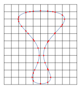
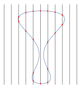
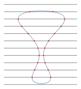
In this example we illustrate the basic sample $E_{\delta}$ in the case of a plane curve $X\subset\mathbb{R}^{2}$. The basic sample consists of the intersection of $X$ with a square grid with side length $\delta$ filling the plane. To acquire the grid we perturb the standard grid (which has a vertex at the origin) by a random vector. An example curve and its intersection with the grid may be seen in Figure LABEL:fig:curve-gridlines. Let $\pi_{1}$ and $\pi_{2}$ be the projections to the $x$-axis and $y$-axis, respectively. The grid lines may be split in vertical and horizontal lines. The vertical lines correspond to $\pi_{1}^{-1}(g)$ with $g$ in a grid of size $\delta$ on the $x$-axis, see Figure LABEL:fig:curve-vert. Similarly, Figure LABEL:fig:curve-hor shows the intersection of $X$ with the horizontal lines corresponding to $\pi_{2}^{-1}(g)$ with $g$ in a grid on the $y$-axis.

(a)

(b)

(c)

Figure 2. Basic sample of planar curve.

Example 4.2.

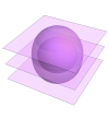
As another example consider the surface $X\subset\mathbb{R}^{3}$ shown in Figure 3. The figure also shows the 1-dimensional skeleton of a cubical complex, or tessellation, filling $\mathbb{R}^{3}$. The tessellation is a random translation of the standard cubical tessellation with cube side length $\delta>0$ and the image is shown from an angle for better visualization. The 1-dimensional skeleton is the union of all the edges of the cubes in the complex and the basic sample $E_{\delta}$ is the intersection of $X$ with the 1-dimensional skeleton. As mentioned above we have in general that the basic sample $E_{\delta}$ of a variety $X\subset\mathbb{R}^{n}$ is the intersection of $X$ with the $\operatorname{codim}(X)$-skeleton of a perturbed cubical complex. In the case of a surface in $\mathbb{R}^{3}$, this intersection may be done by intersecting $X$ with three families of lines as shown in Figures LABEL:fig:surf_xygrid, LABEL:fig:surf_xzgrid and LABEL:fig:surf_yzgrid, respectively. All the lines together are shown in Figure LABEL:fig:surf_fullgrid. These lines can be expressed in terms of projections as follows. Let $\pi_{12}$, $\pi_{13}$ and $\pi_{23}$ be the projections to the $xy$-plane, the $xz$-plane and the $yz$-plane, respectively. Then the lines in Figure LABEL:fig:surf_xygrid are given by $\pi^{-1}_{12}(g)$ with $g$ in a two-dimensional grid in the $xy$-plane like the one shown in Figure LABEL:fig:curve-gridlines. Similarly, the lines in Figures LABEL:fig:surf_xzgrid and LABEL:fig:surf_yzgrid may be expressed using $\pi_{13}$ and $\pi_{23}$, respectively.

(a)

(b)

(c)

(d)

Figure 3. Basic sample of a surface $X\subset\mathbb{R}^{3}$ as intersection of $X$ with the 1-dimensional skeleton of a cubic tessellation.

4.2. The extra sample

In the case $\operatorname{dim}(X)>1$ we need to complement the basic sample with an extra sample $E^{\prime}_{\delta}$ to guarantee density. We will do this without knowing the reach of $X$. For each $1\leq k<d$ we have an extra sample given by

(8) $$E^{\prime}_{\delta,k}=\bigcup_{\begin{subarray}{c}t\in T_{k}\\ g\in G_{t}(\delta)\end{subarray}}I(X\cap\pi_{t}^{-1}(g),q),$$

where $I(X\cap\pi_{t}^{-1}(g),q)$ is the normal locus discussed in Section 2 and $q\in\mathbb{R}^{n}$ is generic. The total extra sample $E^{\prime}_{\delta}$ is the union of $E^{\prime}_{\delta,k}$ for $1\leq k\leq d-1$ and the complete sample of $X$ is

$$S_{\delta}=E_{\delta}\cup E^{\prime}_{\delta}$$

Again, the grid $G_{t}(\delta)$ is perturbed by a random translation which guarantees with probability 1 that the intersections $X\cap\pi_{t}^{-1}(g)$ are smooth for all $g\in G_{t}(\delta)$. Recall that for every connected component $Y$ of $X\cap\pi_{t}^{-1}(g)$, $I(X\cap\pi_{t}^{-1}(g),q)$ contains a point on $Y$. This means that the extra sample $E^{\prime}_{\delta}$ has points of every connected component of $X\cap\pi_{t}^{-1}(g)$ for $g\in G_{t}(\delta)$, $t\in T_{k}$ and $1\leq k\leq d-1$. This will be used below to show density properties of the total sample $S_{\delta}$.

Remark 4.3.

An alternative to introducing the extra sample would be to use only the basic sample but compute the reach of $X$ first and let $\delta$ be small with respect to the reach. The details of showing density requirements for such a simple sampling procedure are yet to be carried out. Moreover the complexity involved in the computation of the reach and in particular the computation of the maximal curvature of $X,$ in the sense explained in Section 2, is to our knowledge still to be explored.

In the case of curves there is no extra sample. For surfaces, the extra sample is constructed by intersecting $X$ with hyperplanes parallel to the coordinate axes and computing normal loci of the resulting curves. In higher dimension we must intersect $X$ with hyperplanes, (codimension 2) planes and so on all the way down to planes of dimension $n-\operatorname{dim}(X)+1$.

Example 4.4.

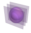
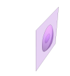
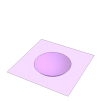
Continuing Example 4.2 we illustrate the extra sample in the case of a surface $X\subset\mathbb{R}^{3}$. The extra sample $E^{\prime}_{\delta}$ is acquired by intersecting $X$ with a number of planes $P\subset\mathbb{R}^{3}$ and computing the normal locus $I(X\cap P,q)$ of the resulting curve. As mentioned above, the normal locus has a point on every connected component of $X\cap P$. The planes come in three families of planes parallel to the $xy$-plane, $xz$-plane and $yz$-plane respectively, see Figure 4. The distance between adjacent planes in the same family is the density parameter $\delta>0$. To tie this to (8), let $\pi_{1}$ be the projection to the $x$-axis and consider for instance the planes parallel to the $yz$-axis. These are expressed in (8) as $\pi_{1}^{-1}(g)$ for $g\in G_{1}(\delta)$ in a grid of size $\delta$ on the $x$-axis.

(a)

(b)

(c)

(d)

(e)

(f)

(g)

(h)

(i)

(j)

(k)

(l)

Figure 4. Extra sample of a surface in $\mathbb{R}^{3}$.

Example 4.5.

In this example we illustrate Algorithm 1 from Section 3.3 by applying it to a simple quadric $X\subset S^{3}\subset\mathbb{R}^{4}$ defined by $xy+y^{2}-2zw=0$ and $x^{2}+y^{2}+z^{2}+w^{2}=1$. We first compute a coarse sample of $X$ (see Figure 5) and evaluate the minimum of $\eta(x)$ over the sample. The result is a bit more than $0.024$.

Figure 5. Quadric in $S^{3}$ projected to $\mathbb{R}^{3}$.

To try to show $0.01<\tau_{X}$ we run Algorithm 1 with $\epsilon_{0}=0.014$ whereby it terminates after producing one sample $E\subset X$. Recall that $E=E_{\delta}\cup E^{\prime}_{\delta}$, where the grid size $\delta$ was chosen to be $\delta=\epsilon_{0}/\sqrt{4}=0.007$.

• Basic sample size: $|E_{\delta}|=780652$

• Extra sample size: $|E^{\prime}_{\delta}|=3592$

• Estimated local reach: $0.024<\min_{e\in E}\eta(e)<0.0246$.

The result is that $\tau_{X}>0.024-0.014=0.01$.

4.3. Density guarantees

In this section we show properties guaranteeing density of the sample $S_{\delta}$ described above.

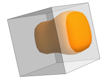
Consider first a surface in $\mathbb{R}^{3}$ as in Example 4.2. The extra sample $E^{\prime}_{\delta}$ is introduced to guarantee density as we will now illustrate. Consider the cubical tessellation underlying the grid and the 1-dimensional skeleton shown in Figure LABEL:fig:surf_fullgrid. If $X$ intersects a cube $\pi$ in the tessellation, we want to have that there is a sample point close by, for example on the boundary $\partial\pi$ of $\pi$. This happens if the basic sample $E_{\delta}$ contains a point on $\partial\pi$. On the other hand, that $E_{\delta}$ has no point on $\partial\pi$ means that the surface $X$ does not intersect any edge of $\pi$. Suppose that we in addition know that no component of $X$ is contained in $\pi$. Then $X$ must intersect the boundary of $\pi$ and the intersection curve has a component $Y$ that is completely contained in one of the faces of $\pi$. See Figure 6 for an illustration. Moreover, $Y$ is a connected component of one of the plane curves $X\cap P$ where $P=\pi_{t}^{-1}(g)$ is one of the planes occurring in the construction of the extra sample (8). As explained above, the extra sample picks up a point on $Y$ which gives a sample point on $\partial\pi$.

We make sure that $X$ has no connected components completely contained in $c$ by choosing the grid size $\delta$ small with respect to the narrowest bottleneck of $X$.

Figure 6. Surface $X\subset\mathbb{R}^{3}$ disjoint from the edges of a cube $\pi$.

Theorem 4.6.

Let $b_{2}$ be the radius of the narrowest bottleneck of $X$ and let $\epsilon>0$. If $0<\delta\sqrt{n}<\min\{\epsilon,2b_{2}\}$, then $S_{\delta}$ is an $\epsilon$-sample of $X$.

Proof.

Let $p\in X$. We must show that there is a point of $S_{\delta}=E_{\delta}\cup E^{\prime}_{\delta}$ at a distance at most $\epsilon$ from $p$. There is a complex $C$ of closed hypercubes (a tessellation) filling $\mathbb{R}^{n}$ such that

$$E_{\delta}=\bigcup_{F\in C_{n-d}}X\cap F$$

where $d=\operatorname{dim}(X)$ and $C_{n-d}$ denotes the set of $(n-d)$-dimensional faces of the hypercubes in $C$. Let $\pi$ be a hypercube in $C$ such that $p\in\pi$. Since the diagonal of $\pi$ has length $\sqrt{n}\delta<\epsilon$, it is enough to find a point in $S_{\delta}\cap\pi$. The diagonal of $\pi$ is shorter than the diameter of the narrowest bottleneck of $X$, which means that no connected component of $X$ can be contained in $\pi$. Hence $X$ intersects the boundary of $\pi$. Any face of $\pi$ of dimension smaller than $n-d$ is contained in some $(n-d)$-dimensional face of $\pi$. Hence, if $x\in X\cap F\neq\emptyset$ for some face $F$ of $\pi$ of dimension $n-d$ or smaller, then $x\in E_{\delta}$ and we are done. This settles the case $d=1$ since no component of $X$ is contained in $\pi$. Now let $F$ be a face of $\pi$ such that $X\cap F\neq\emptyset$ and which has minimal dimension among such faces. By above we may assume $\operatorname{dim}(F)>n-d$. Since $X$ does not intersect the boundary of $F$, $X\cap F$ has a connected component $X_{F}$ that is completely contained in $F$. But then $E^{\prime}_{\delta}$ contains a point $x\in X_{F}$. ∎

4.4. Complexity analysis

As preparatory steps for sampling we need to find a bounding box of $X\subset\mathbb{R}^{n}$ and we need to compute the narrowest bottleneck of $X$. Given a bounding box $B$ of $X$ and a grid size $\delta$ it is straightforward to compute the basic sample $E_{\delta}$ in (7) using standard homotopy methods [2, 30, 3]. We just have to intersect $X$ with the linear spaces $\pi_{t}^{-1}(g)$ for $g\in G_{t}(\delta)\cap\pi_{t}(B)$. Likewise the extra sample $E^{\prime}_{\delta}$ may be computed as explained in Section 2 using for instance multihomogeneous homotopies.

The bounding box may be found by computing the normal locus $I(X,q)$ with respect to a general point $q\in\mathbb{R}^{n}$ as explained in Section 2. Assuming that the bottleneck locus is finite, we may use for example the method presented in [19] to compute the narrowest bottleneck. It is worth noting that the latter method contains as a first step to compute a normal locus $I(X,q)$ so that we may acquire a bounding box from the bottleneck computation alone. In fact, one may derive a bounding box from the widest bottleneck as well if another method to compute bottlenecks is chosen.

To analyze the complexity of computing $E_{\delta}$ and $E^{\prime}_{\delta}$ we count the number of paths that have to be tracked using homotopy continuation methods. To compute $E_{\delta}$ we note that $\#T_{k}={n\choose k}$ and that the number of grid points in $G_{t}(\delta)$ for each $t\in T_{k}$ is $b\delta^{-k}$, where $b$ is the width of the bounding box $B$. By using a parameter homotopy [30], it suffices to solve the system $X\cap L$ where $L$ is a generic affine linear space of complementary dimension and then track deg$(X)$ number of paths to obtain the solutions for each grid point $g\in G_{t}(\delta)$. Let $\#P(X\cap L)$ denote the number of paths that need to be tracked in order to solve the system $X\cap L$. Consequently we would in total have to track $\#P(X\cap L)+{n\choose d}b\delta^{-d}\text{deg}(X)$ number of paths in order to compute the basic sample, since we have ${n\choose d}$ number of grids $G_{t}(\delta)$ and $b\delta^{-k}$ number of grid points for each grid.

Let $L_{k}\subset\mathbb{R}^{n}$ denote a generic affine linear subspace of codimension $k$. For the extra sample we have analogously that we need to track $\#P(I(X\cap L_{k},q))$ number of paths for a generic $q\in\mathbb{R}^{n}$ in order to define the parameter homotopy. The number of solutions for this system is $\text{EDD}(X\cap L_{k})$ and thus we have to track $\sum_{k=1}^{d-1}{n\choose k}b\delta^{-k}\text{EDD}(X\cap L_{k})$ number of paths for the parameter homotopies in order to compute the extra sample. The total number of paths we have to track in order to compute the basic and extra sample using homotopy continuation is thus:

$$\#P(X\cap L)+{n\choose d}b\delta^{-d}\text{deg}(X)+\sum_{k=1}^{d-1}{n\choose k}b\delta^{-k}\text{EDD}(X\cap L_{k})+\#P(I(X\cap L_{k},q))$$

As a final comment we note that the sampling algorithm is parallelizable. The basic sampling can be parallelized over the various projections to coordinate planes as well as the grid points. The extra sample may be parallelized over the linear slices and computations of normal loci. Furthermore, if homotopy methods are used to solve the systems of equations we may parallelize one more aspect of the computation in a straightforward way. Namely, noting that homotopy methods are ultimately path tracking algorithms using prediction/correction, we may parallelize over the paths that need to be tracked.

4.5. Computational comparison

In this section we present a comparison of our sampling method with the sampling method presented in the paper [17] by Dufresne et. al. that also produces a provably dense sampling of algebraic varieties. Due to the spatial structure of their algorithm, an analysis of its complexity is complicated. Their paper does not contain a complexity analysis of their algorithm which makes a theoretical comparison difficult. Because of this we present a computational comparison between the two algorithms where we analyse the number of paths that need to be tracked by a homotopy continuation software. Dufresne et. al. also use parameter homotopies to solve their problem and at each inner loop they have to track EDD$(X)$ number of paths. Note that for convenience we do not consider the number of paths that need to be tracked to compute the generic start point of the parameter homotopy. Due to the structure of their algorithm, analysing the number of paths that have to be tracked is difficult as it relies on spatial data structures. We therefore present the following computational comparison. The varieties in the table below were chosen to be random compact complete intersections of the indicated dimension and degree.

$n$	dim$(X)$	deg$(X)$	$\delta$	# tracked paths		# sample points		total CPU time
				DEHH [17]	DEG	DEHH [17]	DEG	DEHH [17]	DEG
2	1	2	0.5	1184	148	36	58	16s	0.7s
2	1	2	0.1	2940	724	176	294	40s	0.9s
3	2	2	0.5	476814	288	69	149	20m	0.9s
3	2	2	0.1	764688	4698	976	2479	30m	1.4s
4	2	4	0.5	20 467 848	576	75	122	62h	1.3s
4	2	4	0.1	$>10^{8}$	8640	-	2884	$>72$h	3s

Table 1. Computational comparison with the algorithm by Dufresne et. al. [17].

It is clear from the above table that the algorithm by Dufresne et. al. tends to compute a sparser sample, but at a significantly higher cost. As the ambient dimension increases their algorithm breaks down since the number of boxes that need to be checked in the spatial data structure explodes, while our algorithm remains stable.

The experiments for the algorithm by Dufresne et. al. was run using the implementation by Edwards [18] on the Tegner supercomputer at Parallelldatorcentrum (PDC) KTH, using a computational node consisting of 24 Intel E5-2690v3 Haswell cores and 512Gb of RAM. A public implementation of our algorithm is available at [21] and the experiments were run on the same computer as above.

4.6. Experiments

In this section we present some sampling experiments. The equation solving required for the sampling was carried out using numerical homotopy methods with the solver Bertini [2]. The sampled varieties are random complete intersections $X\subset\mathbb{R}^{n}$. To get more interesting examples we choose homogeneous polynomials and to get compact varieties we add a random ellipsoid defined by $\sum_{i=1}^{n}(1+r_{i})x_{i}^{2}=1$ with $r_{i}>0$ random.

We first produce samples of random surfaces in $\mathbb{R}^{4}$ defined by the ellipsoid and a quadratic, cubic, quartic or quintic random polynomial. Coarse samplings projected to $\mathbb{R}^{3}$ of the generated surfaces are shown in Figure 7. In Table 2 we gather some data from the sampling process. The samples produced are $\epsilon$-samples for various $\epsilon$ given in the table. The other columns are the grid size $\delta$, the size of the basic sample $E_{\delta}$ and extra sample $E^{\prime}_{\delta}$ as well as the total CPU time used for all processes. We write the CPU time as $a+b$ where $a$ is the time for computing bottlenecks and $b$ is the time for sampling. For the quadric surface $a$ is less than 5 seconds and is omitted in the table. We implemented the algorithm using eight 1.80 GHz cores of type Intel i7-8550U.

Next we consider random complete intersection surfaces in $\mathbb{R}^{n}$ defined by random quadrics. We conducted the experiments for three surfaces in $\mathbb{R}^{5}$, $\mathbb{R}^{6}$ and $\mathbb{R}^{7}$, respectively. We also did a complete intersection curve in $\mathbb{R}^{6}$ defined by random quadrics. As above we take homogeneous quadrics except for the random ellipsoid which is affine and included in all examples. Coarse samples projected to $\mathbb{R}^{3}$ may be seen in Figure 8. Some sampling data is presented in Table 3 where we, in addition to the fields discussed above, also include the ambient dimension $n$, the dimension of $X$ and the degree of $X$ as a complex variety.

(a)

(b)

(c)

(d)

Figure 7. Plots of sampled surfaces in $\mathbb{R}^{4}$.

$X$	$\epsilon$	$\delta$	$|E_{\delta}|$	$|E^{\prime}_{\delta}|$	total CPU time (m)
Quadric	0.1	0.05	11110	438	5
Quadric	0.02	0.01	269900	2140	122
Quadric	0.01	0.005	1075192	4313	470
Cubic	0.06	0.03	35795	1150	1+26
Cubic	0.02	0.01	315468	3512	1+224
Quartic	0.06	0.03	40390	1026	8+49
Quintic	0.1	0.05	10338	602	95+52

Table 2. Sampling data for surfaces in $\mathbb{R}^{4}$.

(a)

(b)

(c)

(d)

Figure 8. Plots of sampled complete intersection surfaces and a curve.

$n$	$\operatorname{dim}(X)$	$\operatorname{deg}(X_{\mathbb{C}})$	$\epsilon$	$\delta$	$|E_{\delta}|$	$|E^{\prime}_{\delta}|$	total CPU time (m)
5	2	8	0.12	0.05	4428	304	1+22
6	2	16	0.13	0.05	22986	1070	19+70
6	1	32	0.013	0.005	9172	0	6+11
7	2	32	0.027	0.01	801472	8824	155+5192

Table 3. Sampling data for complete intersections $X\subset\mathbb{R}^{n}$ defined by quadrics.

5. Homology guarantees

In this section we show, using the results of [10], that the homology of the thickenings of a compact smooth variety $X$ is controlled by its generalized bottlenecks. We show in Theorem 5.4 that if $\epsilon<wfs(X)$, then the zeroth and first homology of $X$ can be recovered from an $\epsilon$-sample using a modified Vietoris-Rips complex described in Section 5.1.

Computing the weak feature size is a hard problem, but it is lower bounded by the reach of $X$ [8]. The last part of this section we present a variant of the theorem of Niyogi, Smale and Weinberger [27] stating that we can recover the correct homology of $X$ from an $\epsilon$-sample using local estimates of the reach.

5.1. Homology from bottlenecks

Recall the maps $\ell_{k}\colon B_{k}^{\mathbb{R}}\to\mathbb{R}$ from Definition 3.3. Let $L\coloneqq\cup_{k=1}^{EDD(X)}\text{im}(\ell_{k})$ and let $X_{\epsilon}$ denote the $\epsilon$-thickening of $X$ defined as follows:

$$X_{\epsilon}\coloneqq\{y\in\mathbb{R}^{n}\mid\overline{B}_{y}(\epsilon)\cap X\neq\emptyset\}.$$

It is shown in [10, Theorem 1] that if $\epsilon$ is less than the weak feature size of $X$, then $X_{\epsilon}$ is homotopy equivalent to $X$. We show the following result:

Theorem 5.1.

Let $\epsilon_{1}<\epsilon_{2}\in\mathbb{R}$. If $[\epsilon_{1},\epsilon_{2}]\cap L=\emptyset$, then

$$H_{i}(X_{\epsilon_{1}})\cong H_{i}(X_{\epsilon_{2}})$$

In particular, if $\epsilon<wfs(X)$ then $X$ and $X_{\epsilon}$ are homotopy equivalent.

Proof.

Let $\mathbb{B}_{\sigma}$ be an open ball centered at the origin containing the thickening $X_{\epsilon_{2}}$ of $X$. Consider now the sets $Y_{1}\coloneqq\mathbb{B}_{\sigma}\setminus X_{\epsilon_{1}}$ and $Y_{2}\coloneqq\mathbb{B}_{\sigma}\setminus X_{\epsilon_{2}}$. The thickening of $X$ preserves normality and from [10] it follows that the weak feature size of the thickening equals $wfs(Y_{1})=\text{min}\{t-\epsilon_{1}\mid t\in L\text{ and }t>\epsilon_{1}\}$. Now since $[\epsilon_{1},\epsilon_{2}]\cap L=\emptyset$ it follows that $\epsilon_{2}-\epsilon_{1}<wfs(Y_{1})$ and thus by [10, Theorem 1] it follows that $Y_{1}$ and $Y_{2}$ are homotopy equivalent and that $Y_{2}$ is a deformation retract of $Y_{1}$. Consequently, $X_{\epsilon_{1}}$ and $X_{\epsilon_{2}}$ are homotopy equivalent as well.

The latter statement follows from the above arguments and by the fact that $X$ is homotopy equivalent to $X_{\bar{\epsilon}}$ for $\bar{\epsilon}<\tau_{X}$ by [7]. By the same argument as in the previous paragraph, it follows that $X_{\epsilon}$ is homotopy equivalent to $X_{\bar{\epsilon}}$ which is then in turn homotopy equivalent to $X$. ∎

Example 5.2.

Consider the filtration of thickenings $\{X_{\epsilon}\}_{\epsilon\in\mathbb{R}}$ where $X_{\epsilon}\subseteq X_{\epsilon_{2}}$ for $\epsilon_{1}\leq\epsilon_{2}$. Computing the homology of each $X_{\epsilon}$ in the filtration yields a functor sending $\epsilon$ to the $i$th homology group of $X_{\epsilon}$. By the above theorem $H_{i}(X_{\epsilon_{1}})\cong H_{i}(X_{\epsilon_{2}})$ if $[\epsilon_{1},\epsilon_{2}]\cap L=\emptyset$. Thus the values of when the $i$th homology of the filtration $\{X_{\epsilon}\}_{\epsilon\in\mathbb{R}}$ changes is a subset of set $L$. These are called the critical values of the functor. The functors describing the homology of the filtration is in [23] called the barcodes of $X$. We conclude that the above theorem thus implies that the critical values of the barcodes of $X$ is a subset of the sizes of its generalized bottlenecks.

We will now show that the zeroth and first homology of $X$ can be recovered from a $\epsilon$-sample of $X$ for $\epsilon<b_{2}$ in the case when $b_{2}=wfs(X)$. To recover the homology from the sample we make a special Vietoris-Rips construction on the sample and show that the resulting simplicial complex has the same zeroth and first homology as $X$. The intuition is that the part of the reach coming from the curvature of $X$ does not matter for homology and the only thing that matters are the bottlenecks. However, computing the homology of an $\epsilon$-sample of $X$ with $\epsilon<b_{2}$ using e.g. a Vietoris-Rips complex does not immediately work since we run into trouble at the regions of high curvature. We thus have to find a way of excluding their contribution to the homology.

Since we are concerned with only the zeroth and first homology of $X$ we consider only simplices up to dimension two. Let $S$ be the modified Vietoris-Rips complex constructed as follows:

1. there is a 1-simplex between $a,b\in E$ if:

   1. $\bar{B}_{\epsilon}(a)\cap\bar{B}_{\epsilon}(b)\neq\emptyset$ or

   2. there exists a $c\in E$ such that $\bar{B}_{\epsilon}(a)\cap\bar{B}_{\epsilon}(c)\neq\emptyset$, $\bar{B}_{\epsilon}(b)\cap\bar{B}_{\epsilon}(c)\neq\emptyset$ and $\bar{B}_{\sqrt{8}\epsilon}(a)\cap\bar{B}_{\sqrt{8}\epsilon}(b)\neq\emptyset$.

2. there is a 2-simplex between $a,b,c\in E$ if there is a 1-simplex between each pair.

Since $\epsilon<b_{2}$ it follows that condition (1).($ii$) is only satisfied in regions of high curvature. The factor $\sqrt{8}$ ensures that the triangle between $a,b$ and $c$ can fit inside a quarter of a circle of radius $2\epsilon$. This means that if $a,c$ and $b,c$ are both at distance $2\epsilon$ from each other, then the triangle between $a,b$ and $c$ cannot have an angle larger than 90 degrees at $c$.

Let $U(E,\epsilon)$ denote the union of all closed balls $\bar{B}_{\epsilon}(x)$ for $x\in E$. We label a 1-simplex between $a,b\in E$ in $S$ as good if the intersection of $X$ and the smallest closed ball containing both $a$ and $b$ has only one component. This means that the 1-simplex can be deformed in $U(E,\epsilon)$ to a path between $a$ and $b$ lying on $X$. Note that we will only have that the above intersection has two components in regions of high curvature since $\epsilon<b_{2}$. We will show that any 1-simplex in $S$ is homotopic to a path of good edges in $S$. This then implies that the first homology of $S$ and $X$ are the same.

Lemma 5.3.

Any 1-simplex in $S$ is homotopic to a path of good edges in $S$.

Proof.

Let $a,b\in E$ be such that there is a 1-simplex between $a$ and $b$ in $S$ which is not good. Without loss of generality, assume that there is no neighbour $c$ of $b$ such that $b,c$ is a good edge and $d(a,c)<d(a,b)$. If there exist such a $c$ the path $a,c,b$ is homotopic to $a,c$ and since $b,c$ is a good edge we need to show the statement for $a,c$. It then also follows that $a$ is the closest to $b$ of its neighbours with good edges.

Figure 9. Illustration of the case where the angle of the triangle $a,b,c$ is larger than $90$ degrees at $a$.

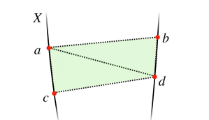
The union $\bar{B}_{\epsilon}(a)\cup\bar{B}_{\epsilon}(b)$ does not contain a bottleneck since $\epsilon<wfs(X)$. It follows that there are $c,d\in E$ such that $a,c$ and $b,d$ are good edges and $d(c,d)<d(a,b)$. If the angle at $a$ of the triangle $a,b,c$ is less than $90$ degrees we have both the 2-simplices $a,b,c$ and $b,d,c$ by condition $(1).(ii)$ in the construction of $S$. Otherwise, if the angle at $a$ is larger than 90 degrees we instead have the 2-simplices $a,c,d$ and $a,b,d$ by condition $(1).(ii)$ and $(2)$. This case is illustrated by Figure 9. Consequently, the path $a,b$ is homotopic to the path $a,c,d,b$ where $a,c$ and $d,b$ are good edges. If $c,d$ is a good edge then we are finished, otherwise we repeat the above argument and since $d(c,d)<d(a,b)$ and the number of samples are finite and $U(E,\epsilon)$ covers $X$ we will eventually terminate, resulting in a path of good edges homotopic to the original 1-simplex. ∎

We use the above lemma to show the following theorem:

Theorem 5.4.

Let $\epsilon<wfs(X)$ and let $i\in\{0,1\}$. Let $E$ be an $\epsilon$-dense sample of $X$ and let $S$ be the modified Vietoris-Rips complex constructed from $E$ as above. Then,

$$H_{i}(S)\cong H_{i}(X)$$

Proof.

The zeroth homology counts the number of components of $X$. Note that the length of the smallest bottleneck of $X$ is smaller or equal to half of the smallest separation between any two components of $X$. Since $U(E,\epsilon)$ covers $X$ and $\epsilon<wfs(X)$ they have the same number of components. The covering $U(E,\epsilon)$ and its Vietoris-Rips complex have the same number of components. It then follows that $U(E,\epsilon)$ and $S$ have the same number of components since condition $1.(ii)$ only adds an edge between vertices who are already connected with an $\epsilon$-path.

First note that since $\epsilon<wfs(X)$ and $U(E,\epsilon)\subseteq X_{\epsilon}$ we have by Theorem 5.1 that it cannot happen that a cycle on $X$ which is not contractible is contractible in $S$ as a cycle of 1-simplices. It therefore remains to show that any cycle of 1-simplices on $S$ is homotopic to a cycle in $X$. This follows from Lemma 5.3. Since any 1-simplex of $S$ is homotopic to a path of good 1-simplices it follows by definition that it can be deformed to lie on $X$. This implies that any 1-cycle on $S$ can be deformed to lie on $X$. Since we also have that $U(E,\epsilon)$ covers $X$ and $\epsilon<wfs(X)$ it follows that any 1-cycle on $X$ can be deformed in $U(E,\epsilon)$ to lie on a subset of the 1-simplices of $S$. We thus have and isomorphism $H_{1}(S)\cong H_{1}(X)$. ∎

In the following example we illustrate the difference between using the density given by the reach and by smallest bottleneck, in the case when $b_{2}=wfs(X)$. For varieties with regions of high curvature this can make a significant difference.

Example 5.5.

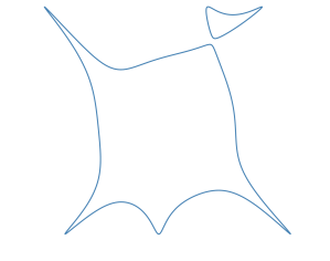
Consider the curve $X\subset\mathbb{R}^{2}$ in the example [5] illustrated by Figure 10 and given by the equation:

$$(x^{3}-xy^{2}+y+1)^{2}(x^{2}+y^{2}-1)+y^{2}-5=0$$

As noted in Section 2, the reach can be expressed as the minimum

$$\tau_{X}=\text{min}\{\frac{1}{\rho},b_{2}\}$$

where $\rho$ is the maximal curvature and $b_{2}$ is the radius of the narrowest bottleneck of $X$. Computing these quantities yields

$$\rho\approx 2097.17,\ \ b_{2}\approx 0.13835$$

which yields that $\tau_{X}\approx 4.79\cdot 10^{-4}$. Using [7, Proposition 2.2], to recover the correct homology of $X$ we thus need a sampling density of $\epsilon<\tau_{X}\approx 4.79\cdot 10^{-4}$. By Theorem 5.4 it suffices to choose the sampling density $\epsilon<b_{2}\approx 0.0692$. By Theorem 4.6 we should then choose the grid size $\delta$ less than $\frac{\epsilon}{\sqrt{n}}$. The sampling algorithm returns the following number of sample points for each of the above densities:

$\delta$	$|E_{\delta}|$
$0.0489$	574
$3.71\cdot 10^{-4}$	58070

Table 4. Comparison of $|E_{\delta}|$ when the density is given by $b_{2}$ and $\tau_{X}$ respectively.

Note in the above table that we need significantly less number of sample points in order to recover the correct homology of $X$ when the density is given by the smallest bottleneck instead of the reach.

Figure 10. The curve $X\subset\mathbb{R}^{2}$ in the example [5].

5.2. Homology using reach

Let $X\subset\mathbb{R}^{n}$ be a smooth compact variety. In this section we present a variant of many statements that appear in the literature of this topic, see for example [7, 27, 9]. Roughly speaking, these results show that a C̆ech complex associated to a dense and accurate enough sample of $X$ deformation retracts onto $X$. In particular $X$ and the complex have the same homology groups which gives an algorithm to compute the homology. Given a finite $\epsilon$-sample $E\subset X$ we have the open cover $X\subseteq\bigcup_{e\in E}B_{e}(\epsilon)$ of open balls with radius $\epsilon$. The C̆ech complex $C(E,\epsilon)$ is the nerve associated to this cover. This means that the simplices of the complex are the subsets $\sigma\subseteq E$ such that $\bigcap_{e\in\sigma}B_{e}(\epsilon)\neq\emptyset$. Our reasoning follows the proof of Theorem 2.8 of [7] closely with the difference that $\epsilon$ is compared to the local reach along the sample $E$ rather than the global reach. This way we may find a complex with the same homology groups as $X$ using a sample of the manifold $X$ rather than a grid in the ambient space $S^{n-1}$ as is done in [7].

Theorem 5.6.

If $E\subset X$, $\epsilon>0$, $E$ is $(\epsilon/2)$-dense and $\epsilon<\frac{4}{5}\tau_{X}(e)$ for all $e\in E$, then $X$ is a deformation retract of $C(E,\epsilon)$. In particular, $X$ and $C(E,\epsilon)$ have the same homology groups.

Proof.

By the assumption $\epsilon<\tau_{X}(e)$ for all $e\in X$, the projection $\pi_{X}:C(E,\epsilon)\rightarrow X$ is well defined and it is continuous by [7] Proposition 2.2. We will show that $(t\pi_{X}(x)+(1-t)x)\in C(E,\epsilon)$ for all $x\in C(E,\epsilon)$. Once this is established the deformation retraction is, as in [7, 27, 9], defined by

$$C(E,\epsilon)\times[0,1]\rightarrow C(E,\epsilon):(x,t)\mapsto t\pi_{X}(x)+(1-t)x.$$

For $a,b\in\mathbb{R}^{n}$, let $[a,b]=\{tb+(1-t)a:t\in[0,1]\}$ and define $[a,b)$, $(a,b]$ and $(a,b)$ similarly by excluding the indicated end points. Let $e\in E$, let $B=B_{e}(\epsilon)\subseteq C(E,\epsilon)$ and let $x\in B$. We need to show that $[x,\pi_{X}(x)]\subseteq C(E,\epsilon)$. If $\pi_{X}(x)\in B$ we are done since then $[x,\pi_{X}(x)]\subseteq B$. Assume that $\pi_{X}(x)\notin B$ and let $L$ be the line joining $x$ and $\pi_{X}(x)$. Since $L$ intersects $B$, it intersects the boundary $\partial B$ in two distinct points on $L$. Call these $p\in L$ and $q\in L$ were $p$ is closer to $\pi_{X}(x)$ than $q$. We need to show that $||p-\pi_{X}(x)||<\epsilon/2$. Once this has been proven we may reason as follows. Since $E$ is $(\epsilon/2)$-dense, there is a $e^{\prime}\in E$ such that $||\pi_{X}(x)-e^{\prime}||<\epsilon/2$. This means that $\pi_{X}(x)\in B_{e^{\prime}}(\epsilon)$ and $p\in B_{e^{\prime}}(\epsilon)$ by the triangle inequality. Hence $[p,\pi_{X}(x)]\subset B_{e^{\prime}}(\epsilon)$. But $[x,p)\subset B_{e}(\epsilon)$ and hence $[x,\pi_{X}(x)]\subset C(E,\epsilon)$.

Let $y=\pi_{X}(x)$, $v=x-y$ and $\tau=\sup\{t\in\mathbb{R}:\pi_{X}(y+tv)=y\}$. Then $0<\tau$ since $\pi_{X}(x)=y$. Moreover, $\tau<\infty$ since if $t_{0}\in\mathbb{R}$ is the unique real number such that $y+t_{0}v$ intersects the hyperplane $\{u\in\mathbb{R}^{n}:||u-e||=||u-y||\}$, then $\tau\leq t_{0}$ since $e\in X$. Put $z=y+\tau v$. By [20] Theorem 4.8 (6), $z$ lies in the medial axis of $X$ and hence $||e-z||\geq\tau_{X}(e)>\frac{5}{4}\epsilon$. Also, by the definition of $\tau$, $||z-y||\leq||z-e||$. We need to show $||y-p||<\epsilon/2$ so assume that $||y-p||\geq\epsilon/2$. Then $||p-z||=||y-z||-||y-p||\leq||z-e||-\epsilon/2$. Since the line segment $(q,p)$ is inside the bass $B_{e}(\epsilon)$, the angle at $p$ of the triangle formed by $e,p$ and $z$ is acute. If follows from the cosine theorem that

$$||e-z||^{2}\leq||p-e||^{2}+||p-z||^{2}=\epsilon^{2}+||p-z||^{2}\leq\epsilon^{2}+(||z-e||-\epsilon/2)^{2}.$$

Hence

$$||e-z||^{2}\leq\epsilon^{2}+||z-e||^{2}-||z-e||\epsilon+\epsilon^{2}/4$$

which implies that $||z-e||\leq\frac{5}{4}\epsilon$, a contradiction. ∎

References

- [1] E. Aamari, F. Chazal, J. Kim, B. Michel, A. Rinaldo, and L. Wasserman. Estimating the reach of a manifold. Electron. J. Statist., 13(1):1359–1399, 2019.
- [2] D.J. Bates, J.D. Hauenstein, A.J. Sommese, and C.W. Wampler. Bertini: Software for numerical algebraic geometry. dx.doi.org/10.7274/R0H41PB5.
- [3] D.J. Bates, J.D. Hauenstein, A.J. Sommese, and C.W. Wampler. Numerically Solving Polynomial Systems with Bertini. SIAM, 2013.
- [4] Paul Breiding and Orlando Marigliano. Random points on an algebraic manifold. arxiv: 1810.06271, 2019.
- [5] Paul Breiding and Sascha Timme. The reach of a plane curve. https://www.JuliaHomotopyContinuation.org/examples/reach-curve/. Accessed: November 5, 2019.
- [6] Paul Breiding and Sascha Timme. Homotopycontinuation.jl: A package for homotopy continuation in julia. In International Congress on Mathematical Software, pages 458–465. Springer, 2018.
- [7] Peter Bürgisser, Felipe Cucker, and Pierre Lairez. Computing the homology of basic semialgebraic sets in weak exponential time. J. ACM, 66:5:1–5:30, 2017.
- [8] Frédéric Chazal, David Cohen-Steiner, and André Lieutier. A sampling theory for compact sets in euclidean space. Discrete & Computational Geometry, 41(3):461–479, Apr 2009.
- [9] Frédéric Chazal and André Lieutier. Weak feature size and persistent homology: Computing homology of solids in rn from noisy data samples. In Proceedings of the Twenty-first Annual Symposium on Computational Geometry, SCG ’05, pages 255–262, New York, NY, USA, 2005. ACM.
- [10] Frédéric Chazal and André Lieutier. The “-medial axis”. Graph. Models, 67(4):304–331, July 2005.
- [11] Mahdi Cheraghchi and Amin Shokrollahi. Almost-uniform sampling of points on high-dimensional algebraic varieties, 2009.
- [12] E.A. Coutsias, S. Martin, and J.P. Thompson, A. Watson. Topology of cyclo-octane energy landscape. J. Chem Phys., 132(234115), 2010.
- [13] Felipe Cucker, Teresa Krick, and Michael Shub. Computing the homology of real projective sets. Foundations of Computational Mathematics, 18(4):929–970, Aug 2018.
- [14] Sandra Di Rocco, David Eklund, Andrew J. Sommese, and Charles W. Wampler. Algebraic -actions and the inverse kinematics of a general 6R manipulator. Appl. Math. Comput., 216(9):2512–2524, 2010.
- [15] Sandra Di Rocco, David Eklund, and Madeleine Weinstein. The bottleneck degree of algebraic varieties. SIAM Journal on Applied Algebra and Geometry, 4(1):227–253, 2020.
- [16] Persi Diaconis, Susan Holmes, and Mehrdad Shahshahani. Sampling from a Manifold, volume Volume 10 of Collections, pages 102–125. Institute of Mathematical Statistics, Beachwood, Ohio, USA, 2013.
- [17] E. Dufresne, P.B. Edwards, H.A. Harrington, and J.D. Hauenstein. Sampling real algebraic varieties for topological data analysis. arXiv:1802.07716, 2018.
- [18] Parker Edwards. Package for sampling real algebraic varieties. https://github.com/P-Edwards/tdasampling. Accessed: January 7, 2020.
- [19] D. Eklund. The numerical algebraic geometry of bottlenecks. arXiv:1804.01015, 2018.
- [20] H. Federer. Curvature measures. Transactions of the American Mathematical Society, 93(2):418–491, 1959.
- [21] Oliver Gäfvert. Sampling and homology via bottlenecks. https://www.JuliaHomotopyContinuation.org/examples/sampling_bottlenecks/. Accessed: October 13, 2020.
- [22] J. Harris. Algebraic Geometry. Springer, first edition, 1992.
- [23] Emil Horobeţ and Madeleine Weinstein. Offset hypersurfaces and persistent homology of algebraic varieties. Computer Aided Geometric Design, 74:101767, 2019.
- [24] J. D. Hunter. Matplotlib: A 2d graphics environment. Computing in Science & Engineering, 9(3):90–95, 2007.
- [25] Wolfram Research, Inc. Mathematica, Version 12.0. Champaign, IL, 2019.
- [26] Steven Kleiman and John Landolfi. Geometry and deformation of special schubert varieties. Compositio Mathematica, 23(4):407–434, 1971.
- [27] P. Niyogi, S. Smale, and S. Weinberger. Finding the homology of submanifolds with high confidence from random samples. Discrete Comput. Geom., 39(1-3):419–441, 2008.
- [28] J. M. Selig. Geometric fundamentals of robotics. Monographs in Computer Science. Springer, New York, second edition, 2005.
- [29] M. Shub and S. Smale. Complexity of Bezout’s theorem iv: Probability of success; extensions. SIAM Journal on Numerical Analysis, 33(1):128–148, 1996.
- [30] A. J. Sommese and C. W. Wampler. The Numerical Solution of Systems of Polynomials Arising in Engineering and Science. World Scientific, 2005.