Diagonal unitary and orthogonal symmetries blablabl in quantum theory

Satvik Singh Email: satviksingh2@gmail.com Affiliation: Department of Physical Sciences, Indian Institute of Science Education and Research (IISER) Mohali, Punjab, India.    Ion Nechita Email: nechita@irsamc.ups-tlse.fr Affiliation: Laboratoire de Physique Théorique, Université de Toulouse, CNRS, UPS, France.
Abstract

We analyze bipartite matrices and linear maps between matrix algebras, which are respectively, invariant and covariant, under the diagonal unitary and orthogonal groups’ actions. By presenting an expansive list of examples from the literature, which includes notable entries like the Diagonal Symmetric states and the Choi-type maps, we show that this class of matrices (and maps) encompasses a wide variety of scenarios, thereby unifying their study. We examine their linear algebraic structure and investigate different notions of positivity through their convex conic manifestations. In particular, we generalize the well-known cone of completely positive matrices to that of triplewise completely positive matrices and connect it to the separability of the relevant invariant states (or the entanglement breaking property of the corresponding quantum channels). For linear maps, we provide explicit characterizations of the stated covariance in terms of their Kraus, Stinespring, and Choi representations, and systematically analyze the usual properties of positivity, decomposability, complete positivity, and the like. We also describe the invariant subspaces of these maps and use their structure to provide necessary and sufficient conditions for separability of the associated invariant states.

1 Introduction

In Quantum Theory, the set of entangled bipartite states has a very special role: the presence of genuinely quantum correlations between the two parties allow for significant advantage in various information processing and computing tasks. However, this paradigm suffers from a significant theoretical hurdle because of the computational hardness of deciding whether a bipartite (or multipartite) quantum state is separable or entangled [23]. To overcome the NP-hardness of this decision problem in the most general case, a plethora of entanglement (resp. separability) criteria have been discovered and studied: there are computationally efficient methods for certifying that a given quantum state is entangled (resp. separable). The most useful entanglement criterion is that of the positive partial transposition (PPT) [55, 32], which turns out to be exact for qubit-qubit and qubit-qutrit systems.

Another way to tackle the separability problem is to restrict the decision problem to special classes of bipartite quantum states. Quantum states satisfying some sort of symmetry are the obvious candidates, since they are physically relevant and mathematically tractable, because of their added structure and reduced number of parameters. One canonical situation is that of bipartite quantum states invariant under the tensor product of the standard representation of the unitary group; two cases need to be considered here:

U𝒰(d),ρ=(UU)ρ(UU) or ρ=(UU¯)ρ(UU¯).\forall U\in\mathcal{U}(d),\qquad\rho=(U\otimes U)\rho(U\otimes U)^{*}\quad\text{ or }\quad\rho=(U\otimes\bar{U})\rho(U\otimes\bar{U})^{*}.

These families of quantum states are respectively known as the Werner [65] and the Isotropic [31] states, and correspond to mixtures of the projections on the symmetric and the anti-symmetric subspaces, respectively to mixtures of the maximally mixed state and the maximally entangled state [64, Example 6.10]. For these one-parameter families (two real parameters if one ignores the unit trace normalization), separability, the PPT property, as well as other relevant properties have been characterized, thanks to their simple structure. Importantly, these states correspond, through the Choi-Jamiołkowski isomorphism, to covariant quantum channels, that is

U𝒰(d),Φ(UXU)=U¯Φ(X)U or Φ(UXU)=UΦ(X)U.\forall U\in\mathcal{U}(d),\qquad\Phi(UXU^{*})=\mkern 1.5mu\overline{\mkern-1.5muU\mkern-1.5mu}\mkern 1.5mu\Phi(X)U^{\top}\quad\text{ or }\quad\Phi(UXU^{*})=U\Phi(X)U^{*}.

In this work, we analyze the properties of quantum states and channels which are symmetric with respect to the diagonal unitary and orthogonal groups. These classes of states are described by roughly d2d^{2} real parameters, and are of intermediate complexity between the full-unitary invariant states described above and the full set of bipartite quantum states (requiring order d4d^{4} parameters). We shall consider three situations: the first two correspond to the equations above, with the unitary UU restricted to the class of diagonal unitary matrices (diagonal matrices with arbitrary complex phases), while the third one corresponds to UU being restricted to diagonal orthogonal matrices (diagonal matrices with arbitrary signs). These classes of states, called respectively LDUI, CLDUI, and LDOI, have been introduced in [14, 36, 52]. We provide a detailed analysis of these matrices, from various points of views: linear algebra, convexity, positivity, separability, etc. Further specializations of these matrices have appeared on numerous occasions in the literature; we thus give a unified treatment of these classes of matrices under one umbrella, in an effort to streamline the different proof techniques used previously.

A focal point of our efforts is the separability problem. It turns out that the classes of states we investigate are still rich enough for the separability problem to be intractable [67, 63, 36], but the situation is simpler, since the search space for separable decompositions is smaller. We describe the separability properties of these invariant states in terms of two cones of pairs and triples of matrices, called the pairwise completely positive [36] and the triplewise completely positive [52] cone, respectively. Both these notions can be understood as extensions of the classical case of completely positive matrices [4], which is a key notion in combinatorics and optimization [1]. We borrow and extend techniques from these fields to provide several separability and entanglement criteria for our classes of invariant states. Building upon the present work, a novel approach to detect entanglement using critical graph-theoretic techniques has been developed in [59].

In the latter half of this paper, we switch perspectives and discuss everything from the point of view of linear maps between matrix algebras, using the Choi-Jamiołkowski isomorphism. Quantum channels which are covariant with respect to the action of diagonal unitary matrices have appeared in the literature under the name of “mean unitary conjugation channels” (MUCC) [47, 49], we dub them here DUC, CDUC, DOC, in parallel with the case of bipartite states. The action of these maps on the space of d×dd\times d complex matrices is parameterized by three d×dd\times d complex matrices: A,BA,B and CC (with diagB=diagC=0\operatorname{diag}B=\operatorname{diag}C=0), and has the following form:

Φ(Z)=diag(A|diagZ)+BZ+CZ.\Phi(Z)=\operatorname{diag}(A\ket{\operatorname{diag}Z})+B\odot Z+C\odot Z^{\top}.

We provide several equivalent characterizations of these classes of maps, based on their Choi, Kraus and Stinespring representations. We also focus on the composition properties of these maps, thus revealing intimate connections with the corresponding class of LDOI matrices. As is done for bipartite matrices, we present a survey of some important examples of maps which lie in our class, the most notable among these being the Choi map and all its proposed generalizations. Remarkably, the results obtained in this work are used in [60] to show that the PPT square conjecture holds for the diagonal unitary covariant maps, which contain all Choi-type maps as special cases.

Although the presentation is self-contained, we refer the reader for the background material and the proofs of some results to our previous work [52] as well as to the paper of Johnston and MacLean [36], where the notions of CLDUI and PCP matrices were introduced. The paper has two main parts, one focusing on bipartite matrices, the other one on linear maps. The sections are structured as follows. In Section 2 we review the main background material on invariant states from [52], recalling several key results from this paper. Section 3 contains a list of salient examples, already present in the literature, or new. Sections 4 and 5 deal with the linear, resp. convex structure of the sets of invariant states and the different cones associated with them. In Section 6 we change gears, and focus on linear maps between matrix algebras; completely positive maps, and quantum channels in particular are discussed here. Section 7 contains a list of examples of quantum channels which are of particular interest. In the next two Sections (8 and 9) we discuss, respectively, the special form of Kraus and Stinespring representations of covariant maps, and the structure of their invariant subspaces, which we use to present necessary and sufficient conditions for separability of the corresponding invariant states. We conclude our work with an overview of our results and some directions for future work. At several instances in this paper, we employ the diagrammatic language of boxes and strings to represent tensor equations, in order to ease proofs and make the presentation more visually intuitive. For readers who are unfamiliar with this language, Section 3 of our previous work [52] should suffice for a quick introduction.

2 Local diagonal unitary and orthogonal invariant matrices

In this section, we recall the basic definitions and properties of the families of local diagonal unitary/orthogonal invariant matrices, which were first introduced in [14], and later studied in [36, 52]. For more details and proofs of the results stated here, the reader should refer to our previous work [52, Sections 6,7 and Appendix B]. We start by fixing some basic notation.

We use Dirac’s bra-ket notation to denote column vectors vdv\in\mathbb{C}^{d} as kets |v\ket{v} and their dual row vectors (conjugate transposes) v(d)v^{*}\in(\mathbb{C}^{d})^{*} as bras v|\bra{v}; note that we do not require the kets or the bras to have unit norm. In this notation, the standard inner product vwv^{*}w on d\mathbb{C}^{d} is denoted by v|w\langle v|w\rangle and the rank one matrix vwvw^{*} is denoted by the outer product |vw|\outerproduct{v}{w}. The standard basis in d\mathbb{C}^{d} is denoted by {|i:i[d]}\{\ket{i}:i\in[d]\}, where [d]{1,2,,d}[d]\coloneqq\{1,2,\ldots,d\}. d,d()\mathcal{M}_{d,d^{\prime}}(\mathbb{R}) and d,d()\mathcal{M}_{d,d^{\prime}}(\mathbb{C}) denote the sets of all d×dd\times d^{\prime} real and complex matrices, respectively, with the standard basis {|ij|:i[d],j[d]}\{\outerproduct{i}{j}:i\in[d],j\in[d^{\prime}]\}. If d=dd=d^{\prime}, we write d()d,d()\mathcal{M}_{d}(\mathbb{R})\coloneqq\mathcal{M}_{d,d}(\mathbb{R}) and d()d,d()\mathcal{M}_{d}(\mathbb{C})\coloneqq\mathcal{M}_{d,d}(\mathbb{C}). For a matrix Vd()V\in\mathcal{M}_{d}(\mathbb{C}), VV^{*} and V¯\mkern 1.5mu\overline{\mkern-1.5muV\mkern-1.5mu}\mkern 1.5mu denote its adjoint and entrywise complex conjugate, respectively. We use the Hilbert-Schmidt inner product on d()\mathcal{M}_{d}(\mathbb{C}): A,B=Tr(AB)\langle A,B\rangle=\operatorname{Tr}(A^{*}B). Hadamard (or entrywise) products of vectors |v,|wd\ket{v},\ket{w}\in\mathbb{C}^{d} and matrices V,Wd()V,W\in\mathcal{M}_{d}(\mathbb{C}) are denoted, respectively, by |vw\ket{v\odot w} and VWV\odot W. Transposition on d()\mathcal{M}_{d}(\mathbb{C}) with respect to the standard basis in d\mathbb{C}^{d} is denoted by \top. dsa()\mathcal{M}^{sa}_{d}(\mathbb{C}) denotes the real vector space of all self-adjoint matrices in d()\mathcal{M}_{d}(\mathbb{C}). The convex cones of entrywise non-negative and positive semi-definite matrices in d()\mathcal{M}_{d}(\mathbb{C}) are denoted by 𝖤𝖶𝖯d\mathsf{EWP}_{d} and 𝖯𝖲𝖣d\mathsf{PSD}_{d} respectively.

For a vector |vd\ket{v}\in\mathbb{C}^{d}, diag|vd()\operatorname{diag}\ket{v}\in\mathcal{M}_{d}(\mathbb{C}) is the diagonal matrix with entries equal to that of |v\ket{v}. For a matrix Vd()V\in\mathcal{M}_{d}(\mathbb{C}), we define two kinds of diagonal operations. The first one extracts out the diagonal part of VV and puts it back in matrix form: diagVd()\operatorname{diag}V\in\mathcal{M}_{d}(\mathbb{C}). The second one does the same thing but the result is a vector: |diagVd\ket{\operatorname{diag}V}\in\mathbb{C}^{d}. The above definitions are collected below:

diag|v=i=1dvi|ii|,diagV=i=1dVii|ii|,|diagV=i=1dVii|i.\operatorname{diag}\ket{v}=\sum_{i=1}^{d}v_{i}\outerproduct{i}{i},\qquad\operatorname{diag}V=\sum_{i=1}^{d}V_{ii}\outerproduct{i}{i},\qquad\ket{\operatorname{diag}V}=\sum_{i=1}^{d}V_{ii}\ket{i}. (1)

Vectors |v|w\ket{v}\otimes\ket{w} in the tensor product space dd\mathbb{C}^{d}\otimes\mathbb{C}^{d^{\prime}} are denoted as |vw\ket{vw}. For bipartite matrices Xd()d()X\in\mathcal{M}_{d}(\mathbb{C})\otimes\mathcal{M}_{d^{\prime}}(\mathbb{C}), the partial transposition with respect to the first and second subsystem is denoted by XΓ(id)(X)X^{\text{\reflectbox{$\Gamma$}}}\coloneqq(\top\otimes\operatorname{id})(X) and XΓ(id)(X)X^{\Gamma}\coloneqq(\operatorname{id}\otimes\top)(X) respectively. A matrix Xd()d()X\in\mathcal{M}_{d}(\mathbb{C})\otimes\mathcal{M}_{d^{\prime}}(\mathbb{C}) is said to be PPT if both XX and XΓX^{\Gamma} are positive semi-definite. By utilizing the isomorphism d()d()dd()\mathcal{M}_{d}(\mathbb{C})\otimes\mathcal{M}_{d^{\prime}}(\mathbb{C})\simeq\mathcal{M}_{dd^{\prime}}(\mathbb{C}), we denote the sets of all self-adjoint, entrywise non-negative and positive semi-definite matrices in d()d()\mathcal{M}_{d}(\mathbb{C})\otimes\mathcal{M}_{d^{\prime}}(\mathbb{C}) by ddsa()\mathcal{M}^{sa}_{dd^{\prime}}(\mathbb{C}), 𝖤𝖶𝖯dd\mathsf{EWP}_{dd^{\prime}} and 𝖯𝖲𝖣dd\mathsf{PSD}_{dd^{\prime}} respectively.

The groups of diagonal unitary and diagonal orthogonal matrices in d()\mathcal{M}_{d}(\mathbb{C}) will play a central role in our paper. These are denoted by 𝒟𝒰d\mathcal{DU}_{d} and 𝒟𝒪d\mathcal{DO}_{d} respectively. A random diagonal unitary matrix is a random variable U𝒟𝒰dU\in\mathcal{DU}_{d}, having independent and identically distributed (i.i.d.) complex phases on its diagonal: Ukk=eiθkU_{kk}=e^{i\theta_{k}}, with θ1,θ2,,θd\theta_{1},\theta_{2},\ldots,\theta_{d} i.i.d uniformly in [0,2π][0,2\pi]. Similarly, a random diagonal orthogonal matrix is a random variable O𝒟𝒪dO\in\mathcal{DO}_{d}, having independent and identically distributed real signs on its diagonal: Okk=skO_{kk}=s_{k}, with s1,,sds_{1},\ldots,s_{d} i.i.d uniformly in {±1}\{\pm 1\}.

With all the notation in place, we begin with the most important definition of this section.

Definition 2.1.

A bipartite matrix Xd()d()X\in\mathcal{M}_{d}(\mathbb{C})\otimes\mathcal{M}_{d}(\mathbb{C}) is said to be

  • local diagonal unitary invariant (LDUI) if

    U𝒟𝒰d,(UU)X(UU)=X,\forall U\in\mathcal{DU}_{d},\qquad(U\otimes U)X(U^{*}\otimes U^{*})=X,
  • conjugate local diagonal unitary invariant (CLDUI) if

    U𝒟𝒰d,(UU)X(UU)=X,\forall U\in\mathcal{DU}_{d},\qquad(U\otimes U^{*})X(U^{*}\otimes U)=X,
  • local diagonal orthogonal invariant (LDOI) if

    O𝒟𝒪d,(OO)X(OO)=X.\forall O\in\mathcal{DO}_{d},\qquad(O\otimes O)X(O\otimes O)=X.

The vector subspaces of LDUI, CLDUI and LDOI matrices in d()d()\mathcal{M}_{d}(\mathbb{C})\otimes\mathcal{M}_{d}(\mathbb{C}) are denoted, respectively, by 𝖫𝖣𝖴𝖨d\mathsf{LDUI}_{d}, 𝖢𝖫𝖣𝖴𝖨d\mathsf{CLDUI}_{d} and 𝖫𝖣𝖮𝖨d\mathsf{LDOI}_{d}. We can now begin to set up important bijections between the newly introduced vector spaces and certain families of matrix pairs/triples defined as follows: [52, Propositions 6.4 and 7.2]

d()d×2\displaystyle\mathcal{M}_{d}(\mathbb{C})^{\times 2}_{\mathbb{C}^{d}} {(A,B)d()×d()|diag(A)=diag(B)},\displaystyle\coloneqq\{(A,B)\in\mathcal{M}_{d}(\mathbb{C})\times\mathcal{M}_{d}(\mathbb{C})\,\big|\,\operatorname{diag}(A)=\operatorname{diag}(B)\}, (2)
d()d×3\displaystyle\mathcal{M}_{d}(\mathbb{C})^{\times 3}_{\mathbb{C}^{d}} {(A,B,C)d()×d()×d()|diag(A)=diag(B)=diag(C)}.\displaystyle\coloneqq\{(A,B,C)\in\mathcal{M}_{d}(\mathbb{C})\times\mathcal{M}_{d}(\mathbb{C})\times\mathcal{M}_{d}(\mathbb{C})\,\big|\,\operatorname{diag}(A)=\operatorname{diag}(B)=\operatorname{diag}(C)\}. (3)
Proposition 2.2.

Let d()d×2\mathcal{M}_{d}(\mathbb{C})^{\times 2}_{\mathbb{C}^{d}} and d()d×3\mathcal{M}_{d}(\mathbb{C})^{\times 3}_{\mathbb{C}^{d}} be vector spaces defined in Eqs. (2) and (3), endowed with the usual component-wise addition and scalar multiplication. Then,

  • 𝖫𝖣𝖴𝖨d\mathsf{LDUI}_{d} and 𝖢𝖫𝖣𝖴𝖨d\mathsf{CLDUI}_{d} are isomorphic as vector spaces to d()d×2\mathcal{M}_{d}(\mathbb{C})^{\times 2}_{\mathbb{C}^{d}},

  • 𝖫𝖣𝖮𝖨d\mathsf{LDOI}_{d} is isomorphic as a vector space to d()d×3\mathcal{M}_{d}(\mathbb{C})^{\times 3}_{\mathbb{C}^{d}}.

We take a moment to state the bijections from Proposition 2.2 more explicitly. Notice that given Ad()A\in\mathcal{M}_{d}(\mathbb{C}), A~\widetilde{A} denotes the matrix with zero diagonal but with the same off-diagonal entries as AA: A~:=AdiagA\widetilde{A}:=A-\operatorname{diag}A, or, in coordinates

A~ij={    0,if i=jAij,otherwise .\widetilde{A}_{ij}=\begin{cases}\,\,\,\,0,\quad&\text{if }i=j\\ A_{ij},\quad&\text{otherwise }.\end{cases} (4)
X(1):d()d×2\displaystyle\bullet\quad X^{(1)}:\mathcal{M}_{d}(\mathbb{C})^{\times 2}_{\mathbb{C}^{d}} 𝖫𝖣𝖴𝖨d\displaystyle\rightarrow\mathsf{LDUI}_{d}
(A,C)\displaystyle(A,C) X(A,C)(1)=i,j=1dAij|ijij|+1ijdCij|ijji|,\displaystyle\mapsto X^{(1)}_{(A,C)}\coloneqq\includegraphics[align]{X1-AC.pdf}=\sum_{i,j=1}^{d}A_{ij}\outerproduct{ij}{ij}+\sum_{1\leq i\neq j\leq d}C_{ij}\outerproduct{ij}{ji},
X(2):d()d×2\displaystyle\bullet\quad X^{(2)}:\mathcal{M}_{d}(\mathbb{C})^{\times 2}_{\mathbb{C}^{d}} 𝖢𝖫𝖣𝖴𝖨d\displaystyle\rightarrow\mathsf{CLDUI}_{d}
(A,B)\displaystyle(A,B) X(A,B)(2)=i,j=1dAij|ijij|+1ijdBij|iijj|,\displaystyle\mapsto X^{(2)}_{(A,B)}\coloneqq\includegraphics[align]{X2-AB.pdf}=\sum_{i,j=1}^{d}A_{ij}\outerproduct{ij}{ij}+\sum_{1\leq i\neq j\leq d}B_{ij}\outerproduct{ii}{jj},
X(3):d()d×3\displaystyle\bullet\quad X^{(3)}:\mathcal{M}_{d}(\mathbb{C})^{\times 3}_{\mathbb{C}^{d}} 𝖫𝖣𝖮𝖨d\displaystyle\rightarrow\mathsf{LDOI}_{d}
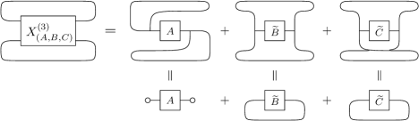
(A,B,C)\displaystyle(A,B,C) X(A,B,C)(3)\displaystyle\mapsto X^{(3)}_{(A,B,C)}\coloneqq\includegraphics[align]{X3-ABC.pdf}
=i,j=1dAij|ijij|+1ijdBij|iijj|+1ijdCij|ijji|.\displaystyle\hskip 58.32823pt=\sum_{i,j=1}^{d}A_{ij}\outerproduct{ij}{ij}+\sum_{1\leq i\neq j\leq d}B_{ij}\outerproduct{ii}{jj}+\sum_{1\leq i\neq j\leq d}C_{ij}\outerproduct{ij}{ji}.

Coordinate-wise, we have (note that X(i1i2,j1j2)=i1i2|X|j1j2X(i_{1}i_{2},j_{1}j_{2})=\langle i_{1}i_{2}|X|j_{1}j_{2}\rangle):

X(A,C)(1)(i1i2,j1j2)\displaystyle X^{(1)}_{(A,C)}(i_{1}i_{2},j_{1}j_{2}) ={Ai1i2, if i1=j1 and i2=j2Ci1j1, if i1=j2 and i2=j10, otherwise\displaystyle=\begin{cases}A_{i_{1}i_{2}},&\quad\text{ if }i_{1}=j_{1}\text{ and }i_{2}=j_{2}\\ C_{i_{1}j_{1}},&\quad\text{ if }i_{1}=j_{2}\text{ and }i_{2}=j_{1}\\ 0,&\quad\text{ otherwise }\end{cases} (5)
X(A,B)(2)(i1i2,j1j2)\displaystyle X^{(2)}_{(A,B)}(i_{1}i_{2},j_{1}j_{2}) ={Ai1i2 if i1=j1 and i2=j2Bi1j1 if i1=i2 and j1=j20, otherwise\displaystyle=\begin{cases}A_{i_{1}i_{2}}&\quad\text{ if }i_{1}=j_{1}\text{ and }i_{2}=j_{2}\\ B_{i_{1}j_{1}}&\quad\text{ if }i_{1}=i_{2}\text{ and }j_{1}=j_{2}\\ 0,&\quad\text{ otherwise }\end{cases} (6)
X(A,B,C)(3)(i1i2,j1j2)\displaystyle X^{(3)}_{(A,B,C)}(i_{1}i_{2},j_{1}j_{2}) ={Ai1i2 if i1=j1 and i2=j2Bi1j1 if i1=i2 and j1=j2Ci1j1 if i1=j2 and i2=j10, otherwise\displaystyle=\begin{cases}A_{i_{1}i_{2}}&\quad\text{ if }i_{1}=j_{1}\text{ and }i_{2}=j_{2}\\ B_{i_{1}j_{1}}&\quad\text{ if }i_{1}=i_{2}\text{ and }j_{1}=j_{2}\\ C_{i_{1}j_{1}}&\quad\text{ if }i_{1}=j_{2}\text{ and }i_{2}=j_{1}\\ 0,&\quad\text{ otherwise }\end{cases} (7)

The general matrix form of a 333\otimes 3 LDOI matrix is exhibited below (dots represent zeros):

X(A,B,C)(3)=(A11ΓΓΓB12ΓΓΓB13ΓA12ΓC12ΓΓΓΓΓΓΓA13ΓΓΓC13ΓΓΓC21ΓA21ΓΓΓΓΓB21ΓΓΓA22ΓΓΓB23ΓΓΓΓΓA23ΓC23ΓΓΓC31ΓΓΓA31ΓΓΓΓΓΓΓC32ΓA32ΓB31ΓΓΓB32ΓΓΓA33).X^{(3)}_{(A,B,C)}=\left(\cdot\begin{array}[]{ *{3}{c} | *{3}{c} | *{3}{c} }A_{11}&0&0&0&B_{12}&0&0&0&B_{13}\\ 0&A_{12}&0&C_{12}&0&0&0&0&0\\ 0&0&A_{13}&0&0&0&C_{13}&0&0\\ \hline\cr 0&C_{21}&0&A_{21}&0&0&0&0&0\\ B_{21}&0&0&0&A_{22}&0&0&0&B_{23}\\ 0&0&0&0&0&A_{23}&0&C_{23}&0\\ \hline\cr 0&0&C_{31}&0&0&0&A_{31}&0&0\\ 0&0&0&0&0&C_{32}&0&A_{32}&0\\ B_{31}&0&0&0&B_{32}&0&0&0&A_{33}\\ \end{array}\right). (8)

We refer the reader to Proposition 4.1 for the block-structure of the above matrices. The next proposition identifies orthogonal projections on the LDUI/CLDUI/LDOI subspaces with certain local diagonal unitary/orthogonal averaging operations [52, Propositions 6.4, 7.2].

Proposition 2.3.

Denote the orthogonal projections on the vector subspaces 𝖫𝖣𝖴𝖨d,𝖢𝖫𝖣𝖴𝖨d\mathsf{LDUI}_{d},\mathsf{CLDUI}_{d} and 𝖫𝖣𝖮𝖨d\mathsf{LDOI}_{d} in d()d()\mathcal{M}_{d}(\mathbb{C})\otimes\mathcal{M}_{d}(\mathbb{C}) by Proj𝖫𝖣𝖴𝖨\operatorname{Proj}_{\mathsf{LDUI}}, Proj𝖢𝖫𝖣𝖴𝖨\operatorname{Proj}_{\mathsf{CLDUI}} and Proj𝖫𝖣𝖮𝖨\operatorname{Proj}_{\mathsf{LDOI}} respectively. For an arbitrary matrix Xd()d()X\in\mathcal{M}_{d}(\mathbb{C})\otimes\mathcal{M}_{d}(\mathbb{C}), define matrices A,B,Cd()A,B,C\in\mathcal{M}_{d}(\mathbb{C}) entrywise as Aij=ij|X|ijA_{ij}=\langle ij|X|ij\rangle, Bij=ii|X|jjB_{ij}=\langle ii|X|jj\rangle, and Cij=ij|X|jiC_{ij}=\langle ij|X|ji\rangle for i,j[d]i,j\in[d]. Then,

Proj𝖫𝖣𝖴𝖨(X)\displaystyle\operatorname{Proj}_{\mathsf{LDUI}}(X) =𝔼U[(UU)X(UU)]=X(A,C)(1),\displaystyle=\mathbb{E}_{U}[(U\otimes U)X(U^{*}\otimes U^{*})]=X^{(1)}_{(A,C)},
Proj𝖢𝖫𝖣𝖴𝖨(X)\displaystyle\operatorname{Proj}_{\mathsf{CLDUI}}(X) =𝔼U[(UU)X(UU)]=X(A,B)(2),\displaystyle=\mathbb{E}_{U}[(U\otimes U^{*})X(U^{*}\otimes U)]=X^{(2)}_{(A,B)},
Proj𝖫𝖣𝖮𝖨(X)\displaystyle\operatorname{Proj}_{\mathsf{LDOI}}(X) =𝔼O[(OO)X(OO)]=X(A,B,C)(3).\displaystyle=\mathbb{E}_{O}[(O\otimes O)X(O\otimes O)]=X^{(3)}_{(A,B,C)}.

where U𝒟𝒰dU\in\mathcal{DU}_{d} (resp. O𝒟𝒪dO\in\mathcal{DO}_{d}) is a random diagonal unitary (resp. orthogonal) matrix, and 𝔼U\mathbb{E}_{U} (resp. 𝔼O\mathbb{E}_{O}) denotes the expectation with respect to the distribution of UU (resp. OO).

We refer the reader to [52, Theorems 4.8 and 5.5] for a nice graphical method to compute general expectations of the form given in Proposition 2.3.

Remark 2.4.

For (A,B)d()d×2(A,B)\in\mathcal{M}_{d}(\mathbb{C})^{\times 2}_{\mathbb{C}^{d}}, the above stated bijections imply that

X(A,B)(1)=X(A,diagA,B)(3),X(A,B)(2)=X(A,B,diagA)(3),[X(A,B)(1)]Γ=X(A,B)(2).X^{(1)}_{(A,B)}=X^{(3)}_{(A,\operatorname{diag}A,B)},\qquad X^{(2)}_{(A,B)}=X^{(3)}_{(A,B,\operatorname{diag}A)},\qquad[X^{(1)}_{(A,B)}]^{\Gamma}=X^{(2)}_{(A,B)}. (9)

Hence, 𝖫𝖣𝖴𝖨d\mathsf{LDUI}_{d} and 𝖢𝖫𝖣𝖴𝖨d\mathsf{CLDUI}_{d} are vector subspaces of 𝖫𝖣𝖮𝖨d\mathsf{LDOI}_{d}.

Next, we introduce the notions of completely positive, pairwise completely positive and triplewise completely positive matrices and link them to the separability problem for matrices in 𝖫𝖣𝖴𝖨d\mathsf{LDUI}_{d}, 𝖢𝖫𝖣𝖴𝖨d\mathsf{CLDUI}_{d} and 𝖫𝖣𝖮𝖨d\mathsf{LDOI}_{d} [52, Lemmas 6.6 and 7.5]. Recall that a positive semi-definite bipartite matrix Xd()d()X\in\mathcal{M}_{d}(\mathbb{C})\otimes\mathcal{M}_{d}(\mathbb{C}) is said to be separable if there exists a family of vectors {|vk,|wk}kId\{\ket{v_{k}},\ket{w_{k}}\}_{k\in I}\subseteq\mathbb{C}^{d} for a finite index set II, such that Eq. (10) holds (observe that VV and WW are matrices in d,|I|()\mathcal{M}_{d,|I|}(\mathbb{C}) with columns given by the vectors {|vk}kI\{\ket{v_{k}}\}_{k\in I} and {|wk}kI\{\ket{w_{k}}\}_{k\in I} respectively). A positive semi-definite Xd()d()X\in\mathcal{M}_{d}(\mathbb{C})\otimes\mathcal{M}_{d}(\mathbb{C}) which is not separable is called entangled.

X=k|vkvk||wkwk|=X=\sum_{k}|v_{k}\rangle\langle v_{k}|\otimes|w_{k}\rangle\langle w_{k}|=\includegraphics[align]{X-sep.pdf} (10)
Definition 2.5 (Completely positive matrices).

A matrix Ad()A\in\mathcal{M}_{d}(\mathbb{R}) is said to be Completely Positive (CP) if there exists an entrywise non-negative matrix V𝖤𝖶𝖯d,dd,d()V\in\mathsf{EWP}_{d,d^{\prime}}\subset\mathcal{M}_{d,d^{\prime}}(\mathbb{R}), for arbitrary dd^{\prime}\in\mathbb{N}, such that the following decomposition holds: A=VVA=VV^{\top}.

We would like to warn the reader at this point that the notion of a completely positive matrix defined above is unrelated from the one of a completely positive map, discussed in Section 6.

Definition 2.6 (Pairwise completely positive matrices).

A matrix pair (A,B)d()d×2(A,B)\in\mathcal{M}_{d}(\mathbb{C})^{\times 2}_{\mathbb{C}^{d}} is said to be Pairwise Completely Positive (PCP) if there exist matrices V,Wd,d()V,W\in\mathcal{M}_{d,d^{\prime}}(\mathbb{C}), for arbitrary dd^{\prime}\in\mathbb{N}, such that the following decomposition holds:

A=(VV¯)(WW¯),B=(VW)(VW).A=(V\odot\mkern 1.5mu\overline{\mkern-1.5muV\mkern-1.5mu}\mkern 1.5mu)(W\odot\mkern 1.5mu\overline{\mkern-1.5muW\mkern-1.5mu}\mkern 1.5mu)^{*},\qquad B=(V\odot W)(V\odot W)^{*}. (11)
Definition 2.7 (Triplewise completely positive matrices).

A matrix triple (A,B,C)d()d×3(A,B,C)\in\mathcal{M}_{d}(\mathbb{C})^{\times 3}_{\mathbb{C}^{d}} is said to be Triplewise Completely Positive (TCP) if there exist matrices V,Wd,d()V,W\in\mathcal{M}_{d,d^{\prime}}(\mathbb{C}), for arbitrary dd^{\prime}\in\mathbb{N}, such that the following decomposition holds:

A=(VV¯)(WW¯),B=(VW)(VW),C=(VW¯)(VW¯).A=(V\odot\mkern 1.5mu\overline{\mkern-1.5muV\mkern-1.5mu}\mkern 1.5mu)(W\odot\mkern 1.5mu\overline{\mkern-1.5muW\mkern-1.5mu}\mkern 1.5mu)^{*},\qquad B=(V\odot W)(V\odot W)^{*},\qquad C=(V\odot\mkern 1.5mu\overline{\mkern-1.5muW\mkern-1.5mu}\mkern 1.5mu)(V\odot\mkern 1.5mu\overline{\mkern-1.5muW\mkern-1.5mu}\mkern 1.5mu)^{*}. (12)

The next result is due to [36, Theorem 3.4], where the authors prove that the notion of PCP matrices generalizes that of CP matrices. In our discussion of partial transpose invariant LDOI matrices in Example 3.5, we will extend this generalization to TCP matrices as well.

Theorem 2.8.

For Ad()A\in\mathcal{M}_{d}(\mathbb{R}), the following equivalence holds: AA is CP (A,A)\iff(A,A) is PCP.

We now arrive at the crucial link between separability of LDOI matrices and the different notions of completely positive matrices introduced.

Theorem 2.9.

Consider a triple (A,B,C)d()d×3(A,B,C)\in\mathcal{M}_{d}(\mathbb{C})^{\times 3}_{\mathbb{C}^{d}}. Then

  • X(A,B)(1)𝖫𝖣𝖴𝖨dX^{(1)}_{(A,B)}\in\mathsf{LDUI}_{d} is separable X(A,B)(2)𝖢𝖫𝖣𝖴𝖨d\iff X^{(2)}_{(A,B)}\in\mathsf{CLDUI}_{d} is separable (A,B)\iff(A,B) is PCP,

  • X(A,B,C)(3)𝖫𝖣𝖮𝖨dX^{(3)}_{(A,B,C)}\in\mathsf{LDOI}_{d} is separable (A,B,C)\iff(A,B,C) is TCP.

Proof.

We prove the equivalence for LDOI matrices, and urge the readers to mimic the same proof for LDUI/CLDUI matrices. Assume first that X(A,B,C)(3)X^{(3)}_{(A,B,C)} is separable and hence can be decomposed as in Eq. (10), with matrices V,Wd,|I|()V,W\in\mathcal{M}_{d,|I|}(\mathbb{C}). Using the coordinate-wise relations in Eq. (7), it is easy to infer the TCP decomposition of (A,B,C)(A,B,C):

=(VV¯)(WW¯),\displaystyle=(V\odot\mkern 1.5mu\overline{\mkern-1.5muV\mkern-1.5mu}\mkern 1.5mu)(W\odot\mkern 1.5mu\overline{\mkern-1.5muW\mkern-1.5mu}\mkern 1.5mu)^{*},
=(VW)(VW),\displaystyle=(V\odot W)(V\odot W)^{*},
=(VW¯)(VW¯).\displaystyle=(V\odot\mkern 1.5mu\overline{\mkern-1.5muW\mkern-1.5mu}\mkern 1.5mu)(V\odot\mkern 1.5mu\overline{\mkern-1.5muW\mkern-1.5mu}\mkern 1.5mu)^{*}.

Conversely, assume that (A,B,C)(A,B,C) is TCP and let V,Wd,d()V,W\in\mathcal{M}_{d,d^{\prime}}(\mathbb{C}) form its TCP decomposition. We construct a separable matrix Xd()d()X\in\mathcal{M}_{d}(\mathbb{C})\otimes\mathcal{M}_{d}(\mathbb{C}) using the V,WV,W matrices, as was done in Eq. (10). It is then not too difficult to see that

X(A,B,C)(3)=𝔼O[(OO)X(OO)]=Proj𝖫𝖣𝖮𝖨(X),X^{(3)}_{(A,B,C)}=\mathbb{E}_{O}[(O\otimes O)X(O\otimes O)]=\operatorname{Proj}_{\mathsf{LDOI}}(X),

and the proof concludes with the observation that since Proj𝖫𝖣𝖮𝖨\operatorname{Proj}_{\mathsf{LDOI}} is a (classically correlated) local operation, it preserves separability (see Proposition 2.3). ∎

Several elementary results on TCP matrix triples are presented in [52, Appendix B]. Some of these results, which will be of relevance to us in later sections, are presented below. Notice that the entrywise and trace (or nuclear) norms on d()\mathcal{M}_{d}(\mathbb{C}) are denoted by .1\|.\|_{1} and .Tr\|.\|_{\operatorname{Tr}} respectively:

X1:=i,j=1d|Xij| and XTr:=TrXX.\|X\|_{1}:=\sum_{i,j=1}^{d}|X_{ij}|\qquad\text{ and }\qquad\|X\|_{\operatorname{Tr}}:=\Tr\sqrt{XX^{*}}.
Lemma 2.10.

Let (A,B,C)d()d×3(A,B,C)\in\mathcal{M}_{d}(\mathbb{C})^{\times 3}_{\mathbb{C}^{d}} be TCP. Then

  1. 1.

    both (A,B)(A,B) and (A,C)(A,C) are PCP,

  2. 2.

    A𝖤𝖶𝖯dA\in\mathsf{EWP}_{d} and B,C𝖯𝖲𝖣dB,C\in\mathsf{PSD}_{d},

  3. 3.

    AijAji|Bij|2A_{ij}A_{ji}\geq|B_{ij}|^{2} and AijAji|Cij|2i,j[d]A_{ij}A_{ji}\geq|C_{ij}|^{2}\,\,\forall i,j\in[d],

  4. 4.

    A1ATrB1BTr\|A\|_{1}-\|A\|_{\operatorname{Tr}}\geq\|B\|_{1}-\|B\|_{\operatorname{Tr}} and A1ATrC1CTr\|A\|_{1}-\|A\|_{\operatorname{Tr}}\geq\|C\|_{1}-\|C\|_{\operatorname{Tr}},

  5. 5.

    A1ATr21i<jdmax{|Bij|,|Cij|}\|A\|_{1}-\|A\|_{\operatorname{Tr}}\geq 2\sum_{1\leq i<j\leq d}\operatorname{max}\{|B_{ij}|,|C_{ij}|\}.

Before proceeding further, it is essential to recall some definitions. A matrix Zd()Z\in\mathcal{M}_{d}(\mathbb{C}) is said to be row (resp. column) diagonally dominant if Ziiji|Zij|Z_{ii}\geq\sum_{j\neq i}|Z_{ij}| for each i[d]i\in[d] (resp. Ziiji|Zji|Z_{ii}\geq\sum_{j\neq i}|Z_{ji}| for each i[d]i\in[d]). A matrix Zd()Z\in\mathcal{M}_{d}(\mathbb{C}) is said to be diagonally dominant if it is both row and column diagonally dominant. The comparison matrix M(Z)M(Z) of ZZ in d()\mathcal{M}_{d}(\mathbb{C}) is defined entrywise as follows:

M(Z)ij={|Zij|,if i=j|Zij|,otherwise .M(Z)_{ij}=\begin{cases}\,\,\,\,|Z_{ij}|,\quad&\text{if }i=j\\ -|Z_{ij}|,\quad&\text{otherwise }.\end{cases} (13)

The next result [36, Theorem 4.4] provides easily verifiable sufficient conditions for a pair (A,B)d()d×2(A,B)\in\mathcal{M}_{d}(\mathbb{C})^{\times 2}_{\mathbb{C}^{d}} to be PCP and hence yields a non-trivial test for separability of the associated matrices in 𝖫𝖣𝖴𝖨d\mathsf{LDUI}_{d} and 𝖢𝖫𝖣𝖴𝖨d\mathsf{CLDUI}_{d}.

Lemma 2.11.

Consider a matrix pair (A,B)d()d×2(A,B)\in\mathcal{M}_{d}(\mathbb{C})^{\times 2}_{\mathbb{C}^{d}} such that A𝖤𝖶𝖯dA\in\mathsf{EWP}_{d}, B𝖯𝖲𝖣dB\in\mathsf{PSD}_{d} and AijAji|Bij|2i,j[d]A_{ij}A_{ji}\geq|B_{ij}|^{2}\,\,\forall i,j\in[d]. Then,

B is diagonally dominant M(B)𝖯𝖲𝖣d(A,B)𝖯𝖢𝖯d.B\text{ is diagonally dominant }\implies M(B)\in\mathsf{PSD}_{d}\implies(A,B)\in\mathsf{PCP}_{d}.

Lemma 2.12 below collects some important properties of matrices in 𝖫𝖣𝖮𝖨d\mathsf{LDOI}_{d} [52, Lemma 7.6]. Analogous results for matrices in 𝖫𝖣𝖴𝖨d\mathsf{LDUI}_{d} and 𝖢𝖫𝖣𝖴𝖨d\mathsf{CLDUI}_{d} can be derived with the help of the following Lemma and Remark 2.4, see [52, Lemmas 6.7 and 6.8]. Recall that if we define the realignment map R:d()d()d()d()R:\mathcal{M}_{d}(\mathbb{C})\otimes\mathcal{M}_{d}(\mathbb{C})\rightarrow\mathcal{M}_{d}(\mathbb{C})\otimes\mathcal{M}_{d}(\mathbb{C}) as R(|ij||kl|)=|ik||jl|i,j[d]R(\outerproduct{i}{j}\otimes\outerproduct{k}{l})=\outerproduct{i}{k}\otimes\outerproduct{j}{l}\,\,\forall i,j\in[d], then all separable matrices Xd()d()X\in\mathcal{M}_{d}(\mathbb{C})\otimes\mathcal{M}_{d}(\mathbb{C}) satisfy: R(X)TrTrX||R(X)||_{\operatorname{Tr}}\leq\operatorname{Tr}X, see [5, 57]. This is known as the realignment criterion of separability. In this paper, we use the notation XR:=R(X)X^{R}:=R(X).

Lemma 2.12.

Consider an arbitrary X(A,B,C)(3)𝖫𝖣𝖮𝖨dX^{(3)}_{(A,B,C)}\in\mathsf{LDOI}_{d}. Then,

  1. 1.

    X(A,B,C)(3)𝖯𝖲𝖣d2A𝖤𝖶𝖯dX^{(3)}_{(A,B,C)}\in\mathsf{PSD}_{d^{2}}\iff A\in\mathsf{EWP}_{d}, B𝖯𝖲𝖣dB\in\mathsf{PSD}_{d}, Cdsa()C\in\mathcal{M}^{sa}_{d}(\mathbb{C}), and AijAji|Cij|2i,j[d]A_{ij}A_{ji}\geq|C_{ij}|^{2}\,\forall i,j\in\penalty\ [d],

  2. 2.

    X(A,B,C)(3)Γ𝖯𝖲𝖣d2A𝖤𝖶𝖯dX^{(3)\,\Gamma}_{(A,B,C)}\in\mathsf{PSD}_{d^{2}}\iff A\in\mathsf{EWP}_{d}, Bdsa()B\in\mathcal{M}^{sa}_{d}(\mathbb{C}), C𝖯𝖲𝖣dC\in\mathsf{PSD}_{d}, and AijAji|Bij|2i,j[d]A_{ij}A_{ji}\geq|B_{ij}|^{2}\,\forall i,j\in\penalty\ [d],

  3. 3.

    X(A,B,C)(3)X^{(3)}_{(A,B,C)} satisfies the realignment criterion \iff condition (5) of Lemma 2.10 holds.

In Quantum Mechanics, states ρ\rho of a physical system (called quantum states) are modelled as bounded operators on a separable Hilbert space \mathcal{H}, i.e., ρ()\rho\in\mathcal{B}(\mathcal{H}), which are positive semi-definite and trace-class with Trρ=1\operatorname{Tr}\rho=1, see [64, Chapter 2], [29, Chapter 2]. For multiparty systems, the Hilbert spaces are naturally required to acquire a tensor product structure, and the relevant states then lie in the space (1n)\mathcal{B}(\mathcal{H}_{1}\otimes\dotsb\otimes\mathcal{H}_{n}). In a finite dimensional bipartite setting: 1d1,2d2\mathcal{H}_{1}\simeq\mathbb{C}^{d_{1}},\mathcal{H}_{2}\simeq\mathbb{C}^{d_{2}}, it is obvious that quantum states of a physical system are just positive semi-definite matrices ρd1()d2()\rho\in\mathcal{M}_{d_{1}}(\mathbb{C})\otimes\mathcal{M}_{d_{2}}(\mathbb{C}) with unit trace. The next lemma exploits the results from Lemma 2.12 to define the class of quantum states within the family of local diagonal orthogonal invariant matrices in d()d()\mathcal{M}_{d}(\mathbb{C})\otimes\mathcal{M}_{d}(\mathbb{C}).

Lemma 2.13.

A matrix X(A,B,C)(3)𝖫𝖣𝖮𝖨dX^{(3)}_{(A,B,C)}\in\mathsf{LDOI}_{d} is a quantum state A𝖤𝖶𝖯d\iff A\in\mathsf{EWP}_{d}, B𝖯𝖲𝖣dB\in\mathsf{PSD}_{d} and Cdsa()C\in\mathcal{M}^{sa}_{d}(\mathbb{C}) such that i,j=1dAij=A1=1\sum_{i,j=1}^{d}A_{ij}=||A||_{1}=1 and AijAji|Cij|2i,j[d]A_{ij}A_{ji}\geq|C_{ij}|^{2}\,\,\forall i,j\in[d].

3 Important classes of LDOI matrices

This section contains a plethora of examples of (classes of) local diagonal orthogonal invariant matrices. We list well-known examples of bipartite quantum states which fit into this category, many classes from the literature, as well as some new ones. The fact that so many examples of bipartite quantum states fit into this framework motivates the study of the general properties of LDOI matrices, which will form the subject matter of Sections 4 and 5 later. We collect all the examples in Table 1 which can be found at the end of this section. In what follows, 𝕀dd()\mathbb{I}_{d}\in\mathcal{M}_{d}(\mathbb{C}) is the identity matrix and 𝕁dd()\mathbb{J}_{d}\in\mathcal{M}_{d}(\mathbb{C}) is the matrix in which all entries are equal to one.

Example 3.1 (Diagonal matrices).


It is easy to see that a bipartite matrix XX lies in 𝖫𝖣𝖴𝖨d𝖢𝖫𝖣𝖴𝖨d\mathsf{LDUI}_{d}\cap\mathsf{CLDUI}_{d} if and only if it is diagonal. The associated triple (A,B,C)d()d×3(A,B,C)\in\mathcal{M}_{d}(\mathbb{C})^{\times 3}_{\mathbb{C}^{d}} then has an arbitrary Ad()A\in\mathcal{M}_{d}(\mathbb{C}) and B=C=diagAB=C=\operatorname{diag}A. In particular, this class contains tensor products of diagonal matrices diag|ydiag|z\operatorname{diag}\ket{y}\otimes\operatorname{diag}\ket{z} with |y,|zd\ket{y},\ket{z}\in\mathbb{C}^{d}, where A=|yz|A=\outerproduct{y}{z}. By fixing |y=|z=|diag𝕀dd\ket{y}=\ket{z}=\ket{\operatorname{diag}\mathbb{I}_{d}}\in\mathbb{C}^{d}, we obtain the identity matrix 𝕀d𝕀d\mathbb{I}_{d}\otimes\mathbb{I}_{d} with A=𝕁dA=\mathbb{J}_{d}. Being diagonal, these matrices are separable if and only if they are PPT if and only if they are positive semi-definite if and only if A𝖤𝖶𝖯dA\in\mathsf{EWP}_{d}.

Example 3.2 (Unit rank and tensor product states).


In this example, we deal with LDOI matrices which factorize either as a unit rank matrix or as a tensor product, see also Remark 4.2.

Proposition 3.1.

The LDOI matrices of unit rank are of the form |YZ|\outerproduct{Y}{Z}, where Y,ZY,Z are either

  • of the ‘diagonal’ form: |Y=i=1dyi|ii\ket{Y}=\sum_{i=1}^{d}y_{i}\ket{ii} and |Z=i=1dzi|ii\ket{Z}=\sum_{i=1}^{d}z_{i}\ket{ii} in dd\mathbb{C}^{d}\otimes\mathbb{C}^{d},

  • or are supported on |ij|ji\mathbb{C}\ket{ij}\oplus\mathbb{C}\ket{ji} for some iji\neq j.

In the former case, B=|yz|B=\outerproduct{y}{z} and A=C=diagBA=C=\operatorname{diag}B, where |y=i=1dyi|i\ket{y}=\sum_{i=1}^{d}y_{i}\ket{i} and |z=i=1dzi|i\ket{z}=\sum_{i=1}^{d}z_{i}\ket{i} are vectors in d\mathbb{C}^{d}, the matrices being CLDUI. In the latter case, the matrices are LDUI. The only unit rank matrices which are simultaneously CLDUI and LDUI are of the form

X=λ|ijij|X=\lambda\outerproduct{ij}{ij} (14)

for some non-zero λ\lambda\in\mathbb{C} and i,j[d]i,j\in[d].

Proof.

Consider a unit rank LDOI matrix X=|YZ|X=\outerproduct{Y}{Z}, with 0|Y,|Zdd0\neq\ket{Y},\ket{Z}\in\mathbb{C}^{d}\otimes\mathbb{C}^{d}. From the LDOI property (see Definition 2.1), we see that for all sign vectors s{±1}ds\in\{\pm 1\}^{d} and all i,j,a,b[d]i,j,a,b\in[d], sisjsasbYijZ¯ab=YijZ¯abs_{i}s_{j}s_{a}s_{b}Y_{ij}\bar{Z}_{ab}=Y_{ij}\bar{Z}_{ab}. This relation holds if |Y\ket{Y} and |Z\ket{Z} are of the diagonal form, in which case

X=i,j=1dyizj¯|iijj|X=\sum_{i,j=1}^{d}y_{i}\mkern 1.5mu\overline{\mkern-1.5muz_{j}\mkern-1.5mu}\mkern 1.5mu\outerproduct{ii}{jj} (15)

is CLDUI. The associated matrices A,BA,B and CC can also be shown to have the required form, see Proposition 2.2 and the bijections following it. If |Y\ket{Y} is not of the diagonal form, then Yij0Y_{ij}\neq 0 for some iji\neq j. This implies that Zab=0Z_{ab}=0 for all (a,b){(i,j),(j,i)}(a,b)\notin\{(i,j),(j,i)\}, and we obtain rank one LDUI matrices of the type

X=(α|ij+β|ji)(γij|+δji|),X=\left(\alpha\ket{ij}+\beta\ket{ji}\right)\left(\gamma\bra{ij}+\delta\bra{ji}\right), (16)

where α,β,γ\alpha,\beta,\gamma and δ\delta are complex numbers. Finally, selecting those matrices from Eqs. (15) and (16) which are both LDUI and CLDUI gives us precisely the matrices in Eq. (14). ∎

Remark 3.2.

The set of LDOI matrices XX having a tensor product structure X=YZX=Y\otimes Z can be deduced from the result above by applying the realignment operation, see the Definition used in Lemma 2.12.

Example 3.3 (Werner and Isotropic matrices).

[65, 31]
A matrix Xd()d()X\in\mathcal{M}_{d}(\mathbb{C})\otimes\mathcal{M}_{d}(\mathbb{C}) is called a Werner (resp. isotropic) matrix if it satisfies (UU)X(UU)=X(U\otimes U)X(U^{*}\otimes U^{*})=X (resp. (UU¯)X(UU¯)=X(U\otimes\mkern 1.5mu\overline{\mkern-1.5muU\mkern-1.5mu}\mkern 1.5mu)X(U\otimes\mkern 1.5mu\overline{\mkern-1.5muU\mkern-1.5mu}\mkern 1.5mu)^{*}=X) for all unitary matrices Ud()U\in\mathcal{M}_{d}(\mathbb{C}). It is obvious from the definition that the Werner matrices lie in 𝖫𝖣𝖴𝖨d\mathsf{LDUI}_{d}, while the isotropic matrices lie in 𝖢𝖫𝖣𝖴𝖨d\mathsf{CLDUI}_{d} (see Definition 2.1). The structure of these matrices is known to be of the following form, for a,ba,b\in\mathbb{C}:

Xa,b𝗐𝖾𝗋=a(𝕀d𝕀d)+bi,j=1d|ijji|,Xa,b𝗂𝗌𝗈=a(𝕀d𝕀d)+bi,j=1d|iijj|.X^{\mathsf{wer}}_{a,b}=a(\mathbb{I}_{d}\otimes\mathbb{I}_{d})+b\sum_{i,j=1}^{d}\outerproduct{ij}{ji},\qquad\qquad X^{\mathsf{iso}}_{a,b}=a(\mathbb{I}_{d}\otimes\mathbb{I}_{d})+b\sum_{i,j=1}^{d}\outerproduct{ii}{jj}. (17)

It is straightforward to check that Xa,b𝗐𝖾𝗋=X(A,B)(1)X^{\mathsf{wer}}_{a,b}=X^{(1)}_{(A,B)} and Xa,b𝗂𝗌𝗈=X(A,B)(2)X^{\mathsf{iso}}_{a,b}=X^{(2)}_{(A,B)}, for A=b𝕀d+a𝕁dA=b\,\mathbb{I}_{d}+a\mathbb{J}_{d} and B=a𝕀d+b𝕁dB=a\mathbb{I}_{d}+b\mathbb{J}_{d}. It is equally easy to see that self-adjointness forces the parameters a,ba,b to be real. Now, observe that B𝖯𝖲𝖣dB\in\mathsf{PSD}_{d} if and only if a0a\geq 0 and det(B)=ad1(a+db)0\operatorname{det}(B)=a^{d-1}(a+db)\geq 0, i.e., B𝖯𝖲𝖣dB\in\mathsf{PSD}_{d} if and only if a0a\geq 0 and ba/db\geq-a/d. Also notice that AijAji|Bij|2i,j[d]A_{ij}A_{ji}\geq|B_{ij}|^{2}\,\,\forall i,j\in[d] if and only if aba-a\leq b\leq a. Combining everything together, we deduce that Xa,b𝗐𝖾𝗋X^{\mathsf{wer}}_{a,b} and Xa,b𝗂𝗌𝗈X^{\mathsf{iso}}_{a,b} are PPT if and only if a0a\geq 0 and a/dba-a/d\leq b\leq a. We now prove that this also suffices to guarantee separability of the concerned matrices.

Proposition 3.3.

Let Xa,b𝗐𝖾𝗋,Xa,b𝗂𝗌𝗈d()d()X^{\mathsf{wer}}_{a,b},X^{\mathsf{iso}}_{a,b}\in\mathcal{M}_{d}(\mathbb{C})\otimes\mathcal{M}_{d}(\mathbb{C}) be the Werner and isotropic matrices, parameterized by the pair (a,b)2(a,b)\in\mathbb{C}^{2}. Then, the following equivalences hold:

Xa,b𝗐𝖾𝗋 is PPTXa,b𝗐𝖾𝗋 is separable\displaystyle X^{\mathsf{wer}}_{a,b}\text{ is \emph{PPT}}\iff X^{\mathsf{wer}}_{a,b}\text{ is separable} Xa,b𝗂𝗌𝗈 is separableXa,b𝗂𝗌𝗈 is PPT\displaystyle\iff X^{\mathsf{iso}}_{a,b}\text{ is separable}\iff X^{\mathsf{iso}}_{a,b}\text{ is \emph{PPT}}
a0 and a/dba.\displaystyle\iff a\geq 0\text{ and }-a/d\leq b\leq a.
Proof.

The idea is to show that the associated pair (A,B)(A,B) is PCP in the range determined by aa and bb. To this end, we first fix a0a\geq 0 and assume that b=a/db=-a/d. It is then evident that BB is diagonally dominant and hence Lemma 2.11 tells us that (A,B)(A,B) is PCP. On the other hand, if b=ab=a, we have

A=B=a𝕀d+a𝕁d=ai=1d|ii|+a|diag𝕀ddiag𝕀d|.A=B=a\mathbb{I}_{d}+a\mathbb{J}_{d}=a\sum_{i=1}^{d}\outerproduct{i}{i}+a\outerproduct{\operatorname{diag}\mathbb{I}_d}{\operatorname{diag}\mathbb{I}_d}.

It is then clear that A=B is CP(A,B)A=B\text{ is CP}\implies(A,B) is PCP, see Theorem 2.8. Separability on the entire interval a/dba-a/d\leq b\leq a then follows from convexity, see also [36, Example 2]. ∎

Example 3.4 (Mixtures of Dicke states or diagonal symmetric matrices).

[67, 63] The symmetric subspace in dd\mathbb{C}^{d}\otimes\mathbb{C}^{d} is spanned by vectors of the form

|ψij={(|ij+|ji)/2,if i<j|ii,if i=j\ket{\psi_{ij}}=\begin{cases}(\ket{ij}+\ket{ji})/\sqrt{2},\quad&\text{if }i<j\\ \,\,\ket{ii},\quad&\text{if }i=j\end{cases} (18)

which constitute what is called the Dicke basis for the symmetric subspace. Bipartite matrices which are diagonal in the Dicke basis are known as diagonal symmetric matrices:

XY𝖽𝗂𝖼𝗄𝖾=1ijdYij|ψijψij|,X^{\mathsf{dicke}}_{Y}=\sum_{1\leq i\leq j\leq d}Y_{ij}\outerproduct{\psi_{ij}}{\psi_{ij}}, (19)

where Yd()Y\in\mathcal{M}_{d}(\mathbb{R}) is an arbitrary symmetric matrix. By defining A=diag(Y)+Y~/2A=\operatorname{diag}(Y)+\widetilde{Y}/2, it becomes clear that XY𝖽𝗂𝖼𝗄𝖾=X(A,A)(1)𝖫𝖣𝖴𝖨dX^{\mathsf{dicke}}_{Y}=X^{(1)}_{(A,A)}\in\mathsf{LDUI}_{d}. From Lemma 2.12, it is evident that XY𝖽𝗂𝖼𝗄𝖾X^{\mathsf{dicke}}_{Y} is PPT if and only if A𝖤𝖶𝖯d𝖯𝖲𝖣d𝖣𝖭𝖭dA\in\mathsf{EWP}_{d}\cap\mathsf{PSD}_{d}\coloneqq\mathsf{DNN}_{d}, i.e., if and only if AA is doubly non-negative. The equivalence of separability of XY𝖽𝗂𝖼𝗄𝖾X^{\mathsf{dicke}}_{Y} and complete positivity of AA can be similarly obtained from Theorem 2.8. Since the convex cones of doubly non-negative and completely positive matrices are equal in dimensions d4d\leq 4 [1, Theorem 2.4], we conclude that XY𝖽𝗂𝖼𝗄𝖾d()d()X^{\mathsf{dicke}}_{Y}\in\mathcal{M}_{d}(\mathbb{C})\otimes\mathcal{M}_{d}(\mathbb{C}) with d4d\leq 4 is separable if and only if it is PPT. For d5d\geq 5, every A𝖣𝖭𝖭dA\in\mathsf{DNN}_{d} which is not completely positive gives rise to a PPT entangled diagonal symmetric matrix.

Example 3.5 (Partial transpose invariant LDOI matrices).


Using Proposition 4.3, it is straightforward to infer that an LDOI matrix is invariant under partial transposition with respect to the first (resp. second) subsystem if and only if the associated triple (A,B,C)d()d×3(A,B,C)\in\mathcal{M}_{d}(\mathbb{C})^{\times 3}_{\mathbb{C}^{d}} satisfies: C=BC=B^{\top} (resp. C=BC=B). Moreover, by definition, these matrices are PPT if and only if they are positive semi-definite, which in turn is equivalent to the condition that A𝖤𝖶𝖯d,B𝖯𝖲𝖣dA\in\mathsf{EWP}_{d},B\in\mathsf{PSD}_{d} and AijAji|Bij|2i,j[d]A_{ij}A_{ji}\geq|B_{ij}|^{2}\,\,\forall i,j\in[d], see Lemma 2.12. Finally, Proposition 3.4 below (combined with Theorem 2.9) shows that separability of these matrices is equivalent to the separability of the corresponding LDUI/CLDUI matrices with matrix pairs (A,B)d()d×2(A,B)\in\mathcal{M}_{d}(\mathbb{C})^{\times 2}_{\mathbb{C}^{d}}.

Proposition 3.4.

For (A,B)d()d×2(A,B)\in\mathcal{M}_{d}(\mathbb{C})^{\times 2}_{\mathbb{C}^{d}}, the following sequence of equivalences hold:

(A,B,B) is TCP(A,B) i\displaystyle(A,B,B^{\top})\text{ is \emph{TCP}}\iff(A,B)\text{ i} PCP(A,B,B) is TCP\displaystyle\text{s \emph{PCP}}\iff(A,B,B)\text{ is \emph{TCP}}
\displaystyle\Big\Updownarrow
(A,B,B) is TCP(A,B) i\displaystyle(A,B^{\top},B)\text{ is \emph{TCP}}\iff(A,B^{\top})\text{ i} PCP(A,B,B) is TCP.\displaystyle\text{s \emph{PCP}}\iff(A,B^{\top},B^{\top})\text{ is \emph{TCP}}.
Proof.

We begin with the first row of equivalences. Since the implications pointing from the ends to the center are trivially obtained from part (1) of Lemma 2.10, we start from the center and assume that (A,B)(A,B) is PCP with V,Wd,d()V,W\in\mathcal{M}_{d,d^{\prime}}(\mathbb{C}) forming its PCP decomposition, see Definition 2.6. Now, define matrices V,W,V′′,W′′d,d()V^{\prime},W^{\prime},V^{\prime\prime},W^{\prime\prime}\in\mathcal{M}_{d,d^{\prime}}(\mathbb{C}) entrywise as follows:

Vij\displaystyle V^{\prime}_{ij} =Vijphase(Wij),\displaystyle=V_{ij}\operatorname{phase}(W_{ij}),\qquad\qquad Wij=|Wij|,\displaystyle W^{\prime}_{ij}=|W_{ij}|,
Vij′′\displaystyle V^{\prime\prime}_{ij} =|Vij|,\displaystyle=|V_{ij}|,\qquad\qquad Wij′′=Wijphase(Vij),\displaystyle W^{\prime\prime}_{ij}=W_{ij}\operatorname{phase}(V_{ij}),

where phase(Vij)\operatorname{phase}(V_{ij}) and phase(Wij)\operatorname{phase}(W_{ij}) are the complex phases of the entries of VV and WW: Vij=|Vij|phase(Vij)V_{ij}=|V_{ij}|\operatorname{phase}(V_{ij}) and Wij=|Wij|phase(Wij)W_{ij}=|W_{ij}|\operatorname{phase}(W_{ij}). Now, observe that since WW^{\prime} is entrywise non-negative (and hence W=W¯W^{\prime}=\mkern 1.5mu\overline{\mkern-1.5muW^{\prime}\mkern-1.5mu}\mkern 1.5mu), V,WV^{\prime},W^{\prime} form a TCP decomposition of (A,B,B)(A,B,B) as in Definition 2.7. Similarly, V′′,W′′V^{\prime\prime},W^{\prime\prime} form a TCP decomposition of (A,B,B)(A,B,B^{\top}). This establishes all the equivalences in the first row. An identical argument does the same for the second row as well. Now, to connect the two rows, we observe that if V,WV,W form a PCP decomposition of (A,B)(A,B), then V′′,W′′¯V^{\prime\prime},\mkern 1.5mu\overline{\mkern-1.5muW^{\prime\prime}\mkern-1.5mu}\mkern 1.5mu (as constructed above) form a PCP decomposition of (A,B)(A,B^{\top}). ∎

Using Proposition 3.4, the conclusion of Theorem 2.8 can be trivially extended to TCP matrices.

Theorem 3.5.

For Ad()A\in\mathcal{M}_{d}(\mathbb{C}), the following equivalences hold:

A is CP(A,A) is PCP(A,A,A) is TCP.A\text{ is \emph{CP}}\iff(A,A)\text{ is \emph{PCP}}\iff(A,A,A)\text{ is \emph{TCP}}.
Example 3.6 (LDOI matrices with A=𝕁dA=\mathbb{J}_{d}).


In Example 3.1, it was shown that 𝕀d𝕀d𝖫𝖣𝖮𝖨d\mathbb{I}_{d}\otimes\mathbb{I}_{d}\in\mathsf{LDOI}_{d} with A=𝕁dA=\mathbb{J}_{d} and B=C=diagA=𝕀dB=C=\operatorname{diag}A=\mathbb{I}_{d}. In this example, we investigate the general class of matrices in 𝖫𝖣𝖮𝖨d\mathsf{LDOI}_{d} with (A,B,C)d()d×3(A,B,C)\in\mathcal{M}_{d}(\mathbb{C})^{\times 3}_{\mathbb{C}^{d}} such that A=𝕁dA=\mathbb{J}_{d}. For the moment, let us restrict ourselves to matrices in 𝖫𝖣𝖴𝖨d\mathsf{LDUI}_{d} and 𝖢𝖫𝖣𝖴𝖨d\mathsf{CLDUI}_{d}. Then, a quick application of Lemma 2.12 is adequate to deduce that such matrices are positive semi-definite if and only if they are PPT if and only if the associated matrix BB is a correlation matrix.

Definition 3.6.

Bd()B\in\mathcal{M}_{d}(\mathbb{C}) is said to be a correlation matrix if B𝖯𝖲𝖣dB\in\mathsf{PSD}_{d} and diagB=𝕀d\operatorname{diag}B=\mathbb{I}_{d}

We collect all d×dd\times d correlation matrices in the set 𝖢𝗈𝗋𝗋d{Z𝖯𝖲𝖣d:diagZ=𝕀d}\mathsf{Corr}_{d}\coloneqq\{Z\in\mathsf{PSD}_{d}\,:\,\operatorname{diag}Z=\mathbb{I}_{d}\}. We now show that for LDUI/CLDUI matrices with A=𝕁dA=\mathbb{J}_{d}, the PPT propetry is equivalent to separability.

Proposition 3.7.

For (𝕁d,B)d()d×2(\mathbb{J}_{d},B)\in\mathcal{M}_{d}(\mathbb{C})^{\times 2}_{\mathbb{C}^{d}}, the following are equivalent for i=1,2i=1,2:

B𝖢𝗈𝗋𝗋dX(𝕁d,B)(i) is PPTX(𝕁d,B)(i) is separable.B\in\mathsf{Corr}_{d}\iff X^{(i)}_{(\mathbb{J}_{d},B)}\text{ is PPT}\iff X^{(i)}_{(\mathbb{J}_{d},B)}\text{ is separable}. (20)
Proof.

The first equivalence is a straightforward consequence of Lemma 2.12 (combined with Remark 2.4): since A=𝕁dA=\mathbb{J}_{d}, the condition 1|Bij|21\geq|B_{ij}|^{2} corresponds to the i,ji,j-minor of BB being non-negative. In the final equivalence, the reverse implication is trivial to obtain. To establish the forward implication, we need to show that B𝖢𝗈𝗋𝗋d(𝕁d,B)B\in\mathsf{Corr}_{d}\implies(\mathbb{J}_{d},B) is PCP (see Theorem 2.9). Hence, assume that B𝖢𝗈𝗋𝗋dB\in\mathsf{Corr}_{d} and consider a decomposition of the form B=WWB=WW^{*}, where Wd,r()W\in\mathcal{M}_{d,r}(\mathbb{C}) with rrank(B)r\geq\operatorname{rank}(B). Now, by choosing V=𝕁d,rV=\mathbb{J}_{d,r} (the d×rd\times r matrix with all entries equal to one), we see that V,WV,W form a PCP decomposition of (𝕁d,B)(\mathbb{J}_{d},B):

[(VV¯)(WW¯)]ij\displaystyle[(V\odot\mkern 1.5mu\overline{\mkern-1.5muV\mkern-1.5mu}\mkern 1.5mu)(W\odot\mkern 1.5mu\overline{\mkern-1.5muW\mkern-1.5mu}\mkern 1.5mu)^{*}]_{ij} =k=1r|Vik|2|Wjk|2=k=1r|Wjk|2=Bjj=1,\displaystyle=\sum_{k=1}^{r}|V_{ik}|^{2}|W_{jk}|^{2}=\sum_{k=1}^{r}|W_{jk}|^{2}=B_{jj}=1,
[(VW)(VW)]ij\displaystyle[(V\odot W)(V\odot W)^{*}]_{ij} =[WW]ij=Bij,\displaystyle=[WW^{*}]_{ij}=B_{ij},

and the proof is complete. ∎

It seems wise to pause here for a moment to collect some useful facts about the set of correlation matrices 𝖢𝗈𝗋𝗋d\mathsf{Corr}_{d} in d()\mathcal{M}_{d}(\mathbb{C}):

  • By definition, Z𝖢𝗈𝗋𝗋dZ𝖯𝖲𝖣dZ\in\mathsf{Corr}_{d}\iff Z\in\mathsf{PSD}_{d} and diagZ=𝕀d\operatorname{diag}Z=\mathbb{I}_{d}.

  • 𝖢𝗈𝗋𝗋d\mathsf{Corr}_{d} is a compact convex set, with the rank one matrices |zz|\outerproduct{z}{z} being the obvious extreme points, for |z𝕋d{|yd:|yi|=1i}\ket{z}\in\mathbb{T}^{d}\coloneqq\{\ket{y}\in\mathbb{C}^{d}:|y_{i}|=1\,\,\forall i\}.

  • For d3d\leq 3, it can be shown that the rank one matrices are the only extreme correlation matrices, and hence 𝖢𝗈𝗋𝗋d=conv{|zz|:|z𝕋d}\mathsf{Corr}_{d}=\operatorname{conv}\{\outerproduct{z}{z}:\ket{z}\in\mathbb{T}^{d}\}. However, for d4d\geq 4, other higher rank extreme points exist, and the preceding conclusion becomes false, see [13, 48, 22, 45].

Now, if we consider the general LDOI matrices with A=𝕁dA=\mathbb{J}_{d}, we can quickly infer that as before, these matrices are PPT if and only if the associated matrices B,C𝖢𝗈𝗋𝗋dB,C\in\mathsf{Corr}_{d}. However, we do not know whether this also suffices to guarantee separability. We do have some partial results in this direction:

  • B𝖢𝗈𝗋𝗋dX(𝕁d,B,B)(3)B\in\mathsf{Corr}_{d}\iff X^{(3)}_{(\mathbb{J}_{d},B,B)} is separable, see Proposition 3.4.

  • B,Cconv{|zz|:|z𝕋d}X(𝕁d,B,C)(3)B,C\in\operatorname{conv}\{\outerproduct{z}{z}:\ket{z}\in\mathbb{T}^{d}\}\implies X^{(3)}_{(\mathbb{J}_{d},B,C)} is separable. Let us quickly prove this. Assume B=|bb|B=\outerproduct{b}{b} and C=|cc|C=\outerproduct{c}{c} are arbitrary rank one correlations, where |b,|c𝕋d\ket{b},\ket{c}\in\mathbb{T}^{d}. Then, we can easily construct vectors |v,|w𝕋d\ket{v},\ket{w}\in\mathbb{T}^{d} such that |vw=|b\ket{v\odot w}=\ket{b} and |vw¯=|c\ket{v\odot\mkern 1.5mu\overline{\mkern-1.5muw\mkern-1.5mu}\mkern 1.5mu}=\ket{c}. Hence, we have 𝕁d=|vv¯ww¯|\mathbb{J}_{d}=\outerproduct{v\odot\overbar{v}}{w\odot\overbar{w}}, B=|vwvw|B=\outerproduct{v\odot w}{v\odot w} and C=|vw¯vw¯|C=\outerproduct{v\odot\overbar{w}}{v\odot\overbar{w}}, implying that (𝕁d,B,C)(\mathbb{J}_{d},B,C) is TCP. The desired result then follows from convexity.

Example 3.7 (Canonical NPT states).


Extraction of maximally entangled states from several copies of a given bipartite quantum state through the use of local operations and classical communication (LOCC) forms a central task in numerous quantum communication and cryptographic protocols. In the asymptotic limit, if a state ρd1()d2()\rho\in\mathcal{M}_{d_{1}}(\mathbb{C})\otimes\mathcal{M}_{d_{2}}(\mathbb{C}) allows for a non-zero rate of extraction (defined as the ratio of the extracted number of maximally entangled states to the number of input states), it is said to be distillable. Non-distillable entangled bipartite states are called bound entangled. It is well known that distillable states ρ\rho are negative under partial transposition (NPT), i.e., (id)ρ(\operatorname{id}\otimes\top)\rho is not positive semi-definite. However, it is not known whether every NPT state is distillable or not. Put differently, the existence of an NPT bound entangled state is uncertain (see the excellent review articles [33, 42] for a more precise formulation of these concepts). In [20], the authors show that every NPT state ρd1()d2()\rho\in\mathcal{M}_{d_{1}}(\mathbb{C})\otimes\mathcal{M}_{d_{2}}(\mathbb{C}) is LOCC-transformable to an NPT state in the following family of states in d()d()\mathcal{M}_{d}(\mathbb{C})\otimes\mathcal{M}_{d}(\mathbb{C}) (dmin(d1,d2)d\leq\operatorname{min}(d_{1},d_{2})), where for iji\neq j, |ψij±=(|ij±|ji)/2\ket{\psi^{\pm}_{ij}}=(\ket{ij}\pm\ket{ji})/\sqrt{2}:

ρa,b,c=ai=1d|iiii|+b1i<jd|ψijψij|+c1i<jd|ψij+ψij+|\rho_{a,b,c}=a\sum_{i=1}^{d}\outerproduct{ii}{ii}+b\sum_{1\leq i<j\leq d}\outerproduct{\psi^-_{ij}}{\psi^-_{ij}}+c\sum_{1\leq i<j\leq d}\outerproduct{\psi^+_{ij}}{\psi^+_{ij}} (21)

and a,b,ca,b,c are real parameters. It is not too hard to discern that the states ρa,b,cd()d()\rho_{a,b,c}\in\mathcal{M}_{d}(\mathbb{C})\otimes\mathcal{M}_{d}(\mathbb{C}) are LDUI, with the associated matrices A,Bd()A,B\in\mathcal{M}_{d}(\mathbb{R}) defined as follows:

Aij={a,if i=j(c+b)/2,otherwise,Bij={a,if i=j(cb)/2,otherwise.A_{ij}=\begin{cases}a,&\text{if }i=j\\ (c+b)/2,&\text{otherwise},\end{cases}\quad B_{ij}=\begin{cases}a,&\text{if }i=j\\ (c-b)/2,&\text{otherwise}.\end{cases} (22)

Hence, to show that every NPT bipartite state is distillable, it suffices to prove distillability for an arbitrary NPT LDUI state in the above family. The parameter ranges within which the above states are PPT/NPT can easily be calculated using Lemma 2.12, see also [20, Figure 2].

Example 3.8 (PPT entangled edge states).


A PPT entangled matrix Xd1()d2()X\in\mathcal{M}_{d_{1}}(\mathbb{C})\otimes\mathcal{M}_{d_{2}}(\mathbb{C}) is said to be an edge state if there are no product vectors |xyrange(X)\ket{xy}\in\operatorname{range}(X) such that |x¯yrange(XΓ)\ket{\mkern 1.5mu\overline{\mkern-1.5mux\mkern-1.5mu}\mkern 1.5muy}\in\operatorname{range}(X^{\Gamma}). These states defy the range criterion of separability in a very extreme fashion [11, 43, 44]. In recent years, there has been a great deal of interest in characterizing edge states XX based on their types, which are nothing but pairs of numbers (p,q)(p,q) such that rank(X)=p\operatorname{rank}(X)=p and rank(XΓ)=q\operatorname{rank}(X^{\Gamma})=q. In particular, for the low dimensional 333\otimes 3 system, all possible types have been identified, and examples for each type have been constructed (see [37] and references therein for a review of all the examples). Noticeably, the authors in [41] show that except for the (4,4)(4,4) type, all other types of 333\otimes 3 edge states can be generated by matrices of the form:

X=(eiθ+eiθΓΓΓeiθΓΓΓeiθΓ1/bΓη|ξΓΓΓΓΓΓΓbΓΓΓζ|ξΓΓΓξ|ηΓbΓΓΓΓΓeiθΓΓΓeiθ+eiθΓΓΓeiθΓΓΓΓΓ1/bΓζ|ηΓΓΓξ|ζΓΓΓ1/bΓΓΓΓΓΓΓη|ζΓbΓeiθΓΓΓeiθΓΓΓeiθ+eiθ)X=\left(\cdot\begin{array}[]{ *{3}{c} | *{3}{c} | *{3}{c} }e^{i\theta}+e^{-i\theta}&0&0&0&-e^{i\theta}&0&0&0&-e^{-i\theta}\\ 0&1/b&0&\langle\eta|\xi\rangle&0&0&0&0&0\\ 0&0&b&0&0&0&\langle\zeta|\xi\rangle&0&0\\ \hline\cr 0&\langle\xi|\eta\rangle&0&b&0&0&0&0&0\\ -e^{-i\theta}&0&0&0&e^{i\theta}+e^{-i\theta}&0&0&0&-e^{i\theta}\\ 0&0&0&0&0&1/b&0&\langle\zeta|\eta\rangle&0\\ \hline\cr 0&0&\langle\xi|\zeta\rangle&0&0&0&1/b&0&0\\ 0&0&0&0&0&\langle\eta|\zeta\rangle&0&b&0\\ -e^{i\theta}&0&0&0&-e^{-i\theta}&0&0&0&e^{i\theta}+e^{-i\theta}\\ \end{array}\right) (23)

where b>0,π/3<θ<π/3(θ0)b>0,\,\,-\pi/3<\theta<\pi/3\,\,(\theta\neq 0) and |η,|ζ,|ξ3\ket{\eta},\ket{\zeta},\ket{\xi}\in\mathbb{C}^{3} are vectors such that

η|η=ζ|ζ=ξ|ξ=eiθ+eiθ,\langle\eta|\eta\rangle=\langle\zeta|\zeta\rangle=\langle\xi|\xi\rangle=e^{i\theta}+e^{-i\theta},
|η|ξ|1,|ξ|ζ|1,|ζ|η|1.|\langle\eta|\xi\rangle|\leq 1,\quad|\langle\xi|\zeta\rangle|\leq 1,\quad|\langle\zeta|\eta\rangle|\leq 1.

The zero pattern of these states immediately reveal that they are all 333\otimes 3 LDOI matrices. The entries of the associated A,BA,B and CC matrices can be read off from the appropriate diagonal/off-diagonal elements of XX.

We summarize all the examples discussed in this section in Table 1.

Ex. Name Defining Characteristic
Ambient
Space
Associated
(A,B,C)(A,B,C)
References
3.1 Diagonal Diagonal matrices in d2()\mathcal{M}_{d^{2}}(\mathbb{C})
𝖫𝖣𝖴𝖨d\mathsf{LDUI}_{d}\,\,\cap
𝖢𝖫𝖣𝖴𝖨d\mathsf{CLDUI}_{d}
Ad()A\in\mathcal{M}_{d}(\mathbb{C})
B=diag(A)B=\operatorname{diag}(A)
3.2 Unit rank
Unit rank LDOI matrices
X=|YZ|X=\outerproduct{Y}{Z}; |Y,|Zdd\ket{Y},\ket{Z}\in\mathbb{C}^{d}\otimes\mathbb{C}^{d}
𝖫𝖣𝖮𝖨d\mathsf{LDOI}_{d}
see
Example 3.2
3.2
Tensor
product
Tensor product LDOI matrices
X=YZX=Y\otimes Z; Y,Zd()Y,Z\in\mathcal{M}_{d}(\mathbb{C})
𝖫𝖣𝖮𝖨d\mathsf{LDOI}_{d}
see
Example 3.2
3.3 Werner
(UU)X(UU)=X(U\otimes U)X(U^{*}\otimes U^{*})=X for
all unitary matrices Ud()U\in\mathcal{M}_{d}(\mathbb{C})
𝖫𝖣𝖴𝖨d\mathsf{LDUI}_{d}
A=b𝕀d+a𝕁dA=b\,\mathbb{I}_{d}+a\mathbb{J}_{d}
C=a𝕀d+b𝕁dC=a\mathbb{I}_{d}+b\mathbb{J}_{d}
a,ba,b\in\mathbb{C}
[65]
3.3 Isotropic
(UU)X(UU)=X(U\otimes U^{*})X(U^{*}\otimes U)=X for
all unitary matrices Ud()U\in\mathcal{M}_{d}(\mathbb{C})
𝖢𝖫𝖣𝖴𝖨d\mathsf{CLDUI}_{d}
A=b𝕀d+a𝕁dA=b\,\mathbb{I}_{d}+a\mathbb{J}_{d}
B=a𝕀d+b𝕁dB=a\mathbb{I}_{d}+b\mathbb{J}_{d}
a,ba,b\in\mathbb{C}
[31]
3.4
Diagonal
symmetric
Diagonal in the Dicke basis of
the dd\mathbb{C}^{d}\otimes\mathbb{C}^{d} symmetric subspace
𝖫𝖣𝖴𝖨d\mathsf{LDUI}_{d}
Ad()A\in\mathcal{M}_{d}(\mathbb{C})
C=AC=A
[63],
[67]
3.5 PT invariant
LDOI matrices invariant under
partial transposition
𝖫𝖣𝖮𝖨d\mathsf{LDOI}_{d}
A,Bd()A,B\in\mathcal{M}_{d}(\mathbb{C})
C=BC=B^{\top} or
C=BC=B
3.6 LDOI A=J LDOI matrices with A=𝕁dA=\mathbb{J}_{d} 𝖫𝖣𝖮𝖨d\mathsf{LDOI}_{d}
A=𝕁dA=\mathbb{J}_{d}
B,Cd()B,C\in\mathcal{M}_{d}(\mathbb{C})
3.7
Canonical
NPT
Every NPT state is LOCC-
transformable to a state in this
class
𝖫𝖣𝖴𝖨d\mathsf{LDUI}_{d}
see
Example 3.7
[20]
3.8 333\otimes 3 edge
333\otimes 3 edge states of all types
except (4,4)(4,4)
𝖫𝖣𝖮𝖨d\mathsf{LDOI}_{d}
see
Example 3.8
[41]
Table 1: Important classes of bipartite matrices in 𝖫𝖣𝖮𝖨d\mathsf{LDOI}_{d}. For more details, see the appropriate examples.

4 Linear structure of LDOI matrices

We discuss in this section the linear structure of the sets of bipartite matrices with the invariance properties discussed in Section 2, focusing on different notions of symmetry. We shall make no reference to any positivity or separability notions, this being the topic of the next section.

It was shown in [52, Sections 6-7] that the sets 𝖢𝖫𝖣𝖴𝖨d\mathsf{CLDUI}_{d}, 𝖫𝖣𝖴𝖨d\mathsf{LDUI}_{d}, 𝖫𝖣𝖮𝖨d\mathsf{LDOI}_{d} are \mathbb{C}-vector spaces with dimensions

dim𝖢𝖫𝖣𝖴𝖨d=dim𝖫𝖣𝖴𝖨d\displaystyle\dim_{\mathbb{C}}\mathsf{CLDUI}_{d}=\dim_{\mathbb{C}}\mathsf{LDUI}_{d} =2d2d,\displaystyle=2d^{2}-d,
dim𝖫𝖣𝖮𝖨d\displaystyle\dim_{\mathbb{C}}\mathsf{LDOI}_{d} =3d22d.\displaystyle=3d^{2}-2d.

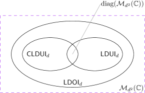
This fact is a consequence of a simple dimension counting for the triples (A,B,C)(A,B,C) using the different diagonal restrictions. For example, in the 𝖢𝖫𝖣𝖴𝖨d\mathsf{CLDUI}_{d} case, the elements are parametrized by pairs (A,B)(A,B) with A,BA,B being d×dd\times d complex matrices (having, in total, 2d22d^{2} complex parameters), with the restriction that diag(A)=diag(B)\operatorname{diag}(A)=\operatorname{diag}(B) (fixing dd complex parameters), resulting in a total of 2d2d2d^{2}-d complex parameters, see Eq. (2) and Proposition 2.2. It is also trivial to see from their definition that 𝖢𝖫𝖣𝖴𝖨d\mathsf{CLDUI}_{d} and 𝖫𝖣𝖴𝖨d\mathsf{LDUI}_{d} are vector subspaces of 𝖫𝖣𝖮𝖨d\mathsf{LDOI}_{d} (see Remark 2.4). Moreover, 𝖢𝖫𝖣𝖴𝖨d𝖫𝖣𝖴𝖨d=diag(d2())\mathsf{CLDUI}_{d}\cap\mathsf{LDUI}_{d}=\operatorname{diag}(\mathcal{M}_{d^{2}}(\mathbb{C})) is precisely the subspace of diagonal matrices in d()d()\mathcal{M}_{d}(\mathbb{C})\otimes\mathcal{M}_{d}(\mathbb{C}), see also Example 3.1. We represent the general position of these vector spaces in Figure 1.

Figure 1: The relative position of the \mathbb{C}-vector spaces 𝖢𝖫𝖣𝖴𝖨d\mathsf{CLDUI}_{d}, 𝖫𝖣𝖴𝖨d\mathsf{LDUI}_{d}, 𝖫𝖣𝖮𝖨d\mathsf{LDOI}_{d}.

As elements of d2()\mathcal{M}_{d^{2}}(\mathbb{C}), the LDUI/CLDUI/LDOI matrices have interesting block structures, which can be derived by using the explicit form of the isomorphisms stated after Proposition 2.2, see also [52, Eq. (41)].

Proposition 4.1.

For all triples (A,B,C)d()d×3(A,B,C)\in\mathcal{M}_{d}(\mathbb{C})^{\times 3}_{\mathbb{C}^{d}}, we have the following decompositions:

X(A,C)(1)\displaystyle X^{(1)}_{(A,C)} =(i[Aii])(i<j[AijCijCjiAji]),\displaystyle=\left(\bigoplus_{i}[A_{ii}]\right)\oplus\left(\bigoplus_{i<j}\begin{bmatrix}A_{ij}&C_{ij}\\ C_{ji}&A_{ji}\end{bmatrix}\right),
X(A,B)(2)\displaystyle X^{(2)}_{(A,B)} =Bij[Aij],\displaystyle=B\oplus\bigoplus_{i\neq j}[A_{ij}],
X(A,B,C)(3)\displaystyle X^{(3)}_{(A,B,C)} =B(i<j[AijCijCjiAji]).\displaystyle=B\oplus\left(\bigoplus_{i<j}\begin{bmatrix}A_{ij}&C_{ij}\\ C_{ji}&A_{ji}\end{bmatrix}\right).
Corollary 4.2.

The rank of the invariant matrices X(1,2,3)X^{(1,2,3)} above are as follows:

rankX(A,C)(1)\displaystyle\operatorname{rank}X^{(1)}_{(A,C)} =|{i[d]:Aii0}|+i<jrank[AijCij,CjiAji]\displaystyle=|\{i\in[d]\,:\,A_{ii}\neq 0\}|+\sum_{i<j}\operatorname{rank}\begin{bmatrix}A_{ij}&C_{ij},\\ C_{ji}&A_{ji}\end{bmatrix}
rankX(A,B)(2)\displaystyle\operatorname{rank}X^{(2)}_{(A,B)} =rankB+|{(i,j)[d]2:ij and Aij0}|,\displaystyle=\operatorname{rank}B+|\{(i,j)\in[d]^{2}\,:\,i\neq j\text{ and }A_{ij}\neq 0\}|,
rankX(A,B,C)(3)\displaystyle\operatorname{rank}X^{(3)}_{(A,B,C)} =rankB+i<jrank[AijCijCjiAji].\displaystyle=\operatorname{rank}B+\sum_{i<j}\operatorname{rank}\begin{bmatrix}A_{ij}&C_{ij}\\ C_{ji}&A_{ji}\end{bmatrix}.

We now consider various symmetries of the vector spaces 𝖫𝖣𝖴𝖨d,𝖢𝖫𝖣𝖴𝖨d\mathsf{LDUI}_{d},\mathsf{CLDUI}_{d} and 𝖫𝖣𝖮𝖨d\mathsf{LDOI}_{d}, obtained by permuting the tensor legs (i.e. the wires in the graphical representation corresponding to the different tensor factors) of the relevant bipartite matrices.

Proposition 4.3.

The vector subspaces 𝖢𝖫𝖣𝖴𝖨d,𝖫𝖣𝖴𝖨d,𝖫𝖣𝖮𝖨dd2()\mathsf{CLDUI}_{d},\mathsf{LDUI}_{d},\mathsf{LDOI}_{d}\subseteq\mathcal{M}_{d^{2}}(\mathbb{C}) are invariant under pairwise leg permutations:

FX(A,B,C)(3)F\displaystyle FX^{(3)}_{(A,B,C)}F =X(A,B,C)(3),(X(A,B,C)(3))\displaystyle=X^{(3)}_{(A^{\top},B,C^{\top})},\qquad\qquad\left(X^{(3)}_{(A,B,C)}\right)^{\top} =X(A,B,C)(3),\displaystyle=X^{(3)}_{(A,B^{\top},C^{\top})},
(X(A,B,C)(3))×\displaystyle\left(X^{(3)}_{(A,B,C)}\right)^{\times} =X(A,B,C)(3),(X(A,B,C)(3))R\displaystyle=X^{(3)}_{(A^{\top},B^{\top},C)},\qquad\qquad\left(X^{(3)}_{(A,B,C)}\right)^{R} =X(B,A,C)(3),\displaystyle=X^{(3)}_{(B,A,C)},

where FF is the flip operator (F|ab=|baF\ket{ab}=\ket{ba}), ×\times permutes the legs of a 4-tensor diagonally and RR is the realignment operation. Moreover, the space 𝖫𝖣𝖮𝖨d\mathsf{LDOI}_{d} has the following additional symmetries:

(X(A,B,C)(3))Γ\displaystyle\left(X^{(3)}_{(A,B,C)}\right)^{\Gamma} =X(A,C,B)(3),FX(A,B,C)(3)\displaystyle=X^{(3)}_{(A,C,B)},\qquad\qquad FX^{(3)}_{(A,B,C)} =X(C,B,A)(3),\displaystyle=X^{(3)}_{(C^{\top},B,A^{\top})},
(X(A,B,C)(3))Γ\displaystyle\left(X^{(3)}_{(A,B,C)}\right)^{\text{\reflectbox{$\Gamma$}}} =X(A,C,B)(3),X(A,B,C)(3)F\displaystyle=X^{(3)}_{(A,C^{\top},B^{\top})},\quad\qquad X^{(3)}_{(A,B,C)}F =X(C,B,A)(3).\displaystyle=X^{(3)}_{(C,B,A)}.
Proof.

All the above relations are easily verified using algebra, but expressing them in the graphical language of tensor networks is more insightful. We leave the detailed proofs to the reader, and provide a graphical proof for the flip FX(A,B,C)(3)FFX^{(3)}_{(A,B,C)}F operation in Figure 2. Finally, Remark 2.4 can be used to derive analogous results for the 𝖢𝖫𝖣𝖴𝖨d\mathsf{CLDUI}_{d} and 𝖫𝖣𝖴𝖨d\mathsf{LDUI}_{d} subspaces.

Figure 2: The conjugation of the LDOI matrix X(A,B,C)(3)X^{(3)}_{(A,B,C)} by the flip operator. The two-sided action of the flip operator on each of the matrices A,B~,C~A,\widetilde{B},\widetilde{C} amounts to transposing the first and the last.
Remark 4.4.

There are more tensor-leg permutations that leave invariant the 𝖫𝖣𝖮𝖨d\mathsf{LDOI}_{d} matrices, by permuting the A,B,CA,B,C matrices and adding transposes to them. The 4!=244!=24 possible leg permutations correspond to 3!×23/23!\times 2^{3}/2 such operations on the ordered triples (A,B,C)(A,B,C), where the 3!3! factor corresponds to permuting the matrices, 232^{3} corresponds to the choice of adding or not a transpose on each letter, and the division by 2 corresponds to the requirement that the number of transposes should be even. We have presented in Proposition 4.3 the most relevant ones for the quantum information theory, see Proposition 6.15 for the corresponding linear map symmetries.

The considerations above allow us to characterize self-adjoint LDOI matrices as follows.

Proposition 4.5.

X(A,B,C)(3)𝖫𝖣𝖮𝖨dX^{(3)}_{(A,B,C)}\in\mathsf{LDOI}_{d} is self-adjoint Ad()\iff A\in\mathcal{M}_{d}(\mathbb{R}) and B,Cdsa()B,C\in\mathcal{M}^{sa}_{d}(\mathbb{C}). In particular, the real vector spaces of self-adjoint invariant matrices have the following dimensions:

dim𝖢𝖫𝖣𝖴𝖨dsa=dim𝖫𝖣𝖴𝖨dsa\displaystyle\dim_{\mathbb{R}}\mathsf{CLDUI}_{d}^{sa}=\dim_{\mathbb{R}}\mathsf{LDUI}_{d}^{sa} =2d2d,\displaystyle=2d^{2}-d,
dim𝖫𝖣𝖮𝖨dsa\displaystyle\dim_{\mathbb{R}}\mathsf{LDOI}_{d}^{sa} =3d22d.\displaystyle=3d^{2}-2d.
Proof.

The main assertion follows from Proposition 4.3:

(X(A,B,C)(3))=(X(A,B,C)(3))¯=X(A,B,C)(3)¯=X(A¯,B,C)(3).\left(X^{(3)}_{(A,B,C)}\right)^{*}=\overline{\left(X^{(3)}_{(A,B,C)}\right)^{\top}}=\overline{X^{(3)}_{(A,B^{\top},C^{\top})}}=X^{(3)}_{(\bar{A},B^{*},C^{*})}.

Proposition 4.6.

A matrix X=X(A,B,C)(3)𝖫𝖣𝖮𝖨dX=X^{(3)}_{(A,B,C)}\in\mathsf{LDOI}_{d} is symmetric (i.e. X=FXFX=FXF) if and only if

A=A and C=C.A=A^{\top}\quad\text{ and }\quad C=C^{\top}.

Moreover, XX is Bose-symmetric (i.e. X=PsXPsX=P_{s}XP_{s}, where PsP_{s} is the orthogonal projection on the symmetric subspace of dd\mathbb{C}^{d}\otimes\mathbb{C}^{d}) if and only if

A=C=A=C.A=C=A^{\top}=C^{\top}.
Proof.

For the first claim, use Proposition 4.3. For the second claim, use Ps=(I+F)/2P_{s}=(I+F)/2 and Proposition 4.3 to get

4A\displaystyle 4A =A+C+C+A,\displaystyle=A+C^{\top}+C+A^{\top},
4C\displaystyle 4C =C+A+A+C,\displaystyle=C+A^{\top}+A+C^{\top},

from which the conclusion immediately follows. ∎

We now show that the 𝖢𝖫𝖣𝖴𝖨d\mathsf{CLDUI}_{d}, 𝖫𝖣𝖴𝖨d\mathsf{LDUI}_{d}, and 𝖫𝖣𝖮𝖨d\mathsf{LDOI}_{d} vector spaces are stable under a modified notion of direct sum, that we introduce next.

Definition 4.7.

Given two bipartite matrices Xidi2()X_{i}\in\mathcal{M}_{d_{i}^{2}}(\mathbb{C}), i=1,2i=1,2, we define their bipartite direct sum X1X2(d1+d2)2()X_{1}\boxplus X_{2}\in\mathcal{M}_{(d_{1}+d_{2})^{2}}(\mathbb{C}) by

[X1X2]((i1,i2),(j1,j2))={X1((i1,i2),(j1,j2)) if i1,i2,j1,j2d1X2((i1d1,i2d1),(j1d1,j2d1)) if i1,i2,j1,j2>d10 otherwise.[X_{1}\boxplus X_{2}]((i_{1},i_{2}),(j_{1},j_{2}))=\begin{cases}X_{1}((i_{1},i_{2}),(j_{1},j_{2}))&\quad\text{ if }i_{1},i_{2},j_{1},j_{2}\leq d_{1}\\ X_{2}((i_{1}-d_{1},i_{2}-d_{1}),(j_{1}-d_{1},j_{2}-d_{1}))&\quad\text{ if }i_{1},i_{2},j_{1},j_{2}>d_{1}\\ 0&\quad\text{ otherwise.}\end{cases}

With this definition in hand, we have the following result, showing that the vector spaces of invariant bipartite matrices are stable under bipartite direct sum.

Proposition 4.8.

Given matrices Ai,Bi,Cidi()A_{i},B_{i},C_{i}\in\mathcal{M}_{d_{i}}(\mathbb{C}), i=1,2i=1,2, the following relations hold:

X(A1,B1)(1)X(A2,B2)(1)\displaystyle X^{(1)}_{(A_{1},B_{1})}\boxplus X^{(1)}_{(A_{2},B_{2})} =X(A1A2,B1B2)(1),\displaystyle=X^{(1)}_{(A_{1}\oplus A_{2},B_{1}\oplus B_{2})},
X(A1,B1)(2)X(A2,B2)(2)\displaystyle X^{(2)}_{(A_{1},B_{1})}\boxplus X^{(2)}_{(A_{2},B_{2})} =X(A1A2,B1B2)(2),\displaystyle=X^{(2)}_{(A_{1}\oplus A_{2},B_{1}\oplus B_{2})},
X(A1,B1,C1)(3)X(A2,B2,C2)(2)\displaystyle X^{(3)}_{(A_{1},B_{1},C_{1})}\boxplus X^{(2)}_{(A_{2},B_{2},C_{2})} =X(A1A2,B1B2,C1C2)(3).\displaystyle=X^{(3)}_{(A_{1}\oplus A_{2},B_{1}\oplus B_{2},C_{1}\oplus C_{2})}.
Proof.

The result directly follows from the explicit (coordinate-wise) expressions of the bijections X(i)X^{(i)} for i=1,2,3i=1,2,3, see Equations (5), (6) and (7). ∎

Remark 4.9.

The fact that the vector spaces of diagonal unitary-invariant matrices are stable under the notion of direct sum defined above is a consequence of the fact that diagonal unitary (resp. orthogonal) matrices of size d1+d2d_{1}+d_{2} are direct sums of diagonal unitary (resp. orthogonal) matrices of sizes d1d_{1} and d2d_{2}. The same does not hold for tensor products, so we do not have a similar stability property with respect to tensor products.

For Ad()A\in\mathcal{M}_{d}(\mathbb{C}) and some index set I[d]I\subset[d], A[I]|I|()A[I]\in\mathcal{M}_{|I|}(\mathbb{C}) denotes the principal submatrix of AA with rows and columns indexed by the indices present in II. In the same vein, for an index set I[d]I\subset[d] and a triple (A,B,C)d()d×3(A,B,C)\in\mathcal{M}_{d}(\mathbb{C})^{\times 3}_{\mathbb{C}^{d}}, we define the principal subtriple of (A,B,C)(A,B,C) associated with the index set II to be the triple (A[I],B[I],C[I])|I|()|I|×3(A[I],B[I],C[I])\in\mathcal{M}_{|I|}(\mathbb{C})^{\times 3}_{\mathbb{C}^{|I|}}. Our next result discusses the effect of this action of taking principal subtriples in the 𝖫𝖣𝖮𝖨d\mathsf{LDOI}_{d} space.

Proposition 4.10.

For a triple (A,B,C)d()d×3(A,B,C)\in\mathcal{M}_{d}(\mathbb{C})^{\times 3}_{\mathbb{C}^{d}} and an index set I[d]I\subset[d], define the projector P=iI|ii|dsa()P=\sum_{i\in I}\outerproduct{i}{i}\in\mathcal{M}^{sa}_{d}(\mathbb{C}). Then, the following relation holds:

(PP)X(A,B,C)(3)(PP)=X(A[I],B[I],C[I])(3),(P\otimes P)X^{(3)}_{(A,B,C)}(P\otimes P)=X^{(3)}_{(A[I],B[I],C[I])},

where the locally projected (PP)X(A,B,C)(3)(PP)(P\otimes P)X^{(3)}_{(A,B,C)}(P\otimes P) is understood to lie in |I|()|I|()\mathcal{M}_{|I|}(\mathbb{C})\otimes\mathcal{M}_{|I|}(\mathbb{C}).

Proof.

Follows trivially from the explicit form of the bijections, stated after Proposition 2.2. ∎

We will see in the next section that the cones of PCP and TCP matrices in d()d×3\mathcal{M}_{d}(\mathbb{C})^{\times 3}_{\mathbb{C}^{d}} are stable under the discussed operations of taking direct sums and principal subtriples. We now conclude this section by discussing the partial actions on 𝖫𝖣𝖮𝖨d\mathsf{LDOI}_{d} of the two conditional expectations on the diagonal and scalar matrices defined below:

diag:d()\displaystyle\operatorname{diag}:\mathcal{M}_{d}(\mathbb{C}) d()trace:d()\displaystyle\to\mathcal{M}_{d}(\mathbb{C})\qquad\qquad\qquad\operatorname{trace}:\mathcal{M}_{d}(\mathbb{C}) d()\displaystyle\to\mathcal{M}_{d}(\mathbb{C})
Z\displaystyle Z\,\, i=1dZii|ii|,Z\displaystyle\mapsto\sum_{i=1}^{d}Z_{ii}\outerproduct{i}{i},\qquad\qquad\qquad\qquad\quad Z TrZdId.\displaystyle\mapsto\frac{\operatorname{Tr}Z}{d}I_{d}.
Proposition 4.11.

For (A,B,C)d()d×3(A,B,C)\in\mathcal{M}_{d}(\mathbb{C})^{\times 3}_{\mathbb{C}^{d}}, define the diagonal matrices A𝗋𝗈𝗐A^{\mathsf{row}} and A𝖼𝗈𝗅A^{\mathsf{col}} in d()\mathcal{M}_{d}(\mathbb{C}) with entries equal to the row and column sums of AA respectively: Aii𝗋𝗈𝗐=j=1dAijA^{\mathsf{row}}_{ii}=\sum_{j=1}^{d}A_{ij} and Aii𝖼𝗈𝗅=j=1dAjii[d]A^{\mathsf{col}}_{ii}=\sum_{j=1}^{d}A_{ji}\,\,\forall i\in[d]. Then, the following relations hold:

[idTr]X(A,B,C)(3)\displaystyle[\operatorname{id}\otimes\operatorname{Tr}]X^{(3)}_{(A,B,C)} =A𝗋𝗈𝗐,\displaystyle=A^{\mathsf{row}},
[Trid]X(A,B,C)(3)\displaystyle[\operatorname{Tr}\otimes\operatorname{id}]X^{(3)}_{(A,B,C)} =A𝖼𝗈𝗅.\displaystyle=A^{\mathsf{col}}.

The action of the partial conditional expectations diag\operatorname{diag} and trace\operatorname{trace} are given respectively by

[iddiag]X(A,B,C)(3)\displaystyle[\operatorname{id}\otimes\operatorname{diag}]X^{(3)}_{(A,B,C)} =X(A,diagA,diagA)(3),[idtrace]X(A,B,C)(3)\displaystyle=X^{(3)}_{(A,\operatorname{diag}A,\operatorname{diag}A)},\qquad\qquad[\operatorname{id}\otimes\operatorname{trace}]X^{(3)}_{(A,B,C)} =1dX(A𝗋𝗈𝗐,A𝗋𝗈𝗐,A𝗋𝗈𝗐)(3),\displaystyle=\frac{1}{d}X^{(3)}_{(A^{\mathsf{row}},A^{\mathsf{row}},A^{\mathsf{row}})},
[diagid]X(A,B,C)(3)\displaystyle[\operatorname{diag}\otimes\operatorname{id}]X^{(3)}_{(A,B,C)} =X(A,diagA,diagA)(3),[traceid]X(A,B,C)(3)\displaystyle=X^{(3)}_{(A,\operatorname{diag}A,\operatorname{diag}A)},\qquad\qquad[\operatorname{trace}\otimes\operatorname{id}]X^{(3)}_{(A,B,C)} =1dX(A𝖼𝗈𝗅,A𝖼𝗈𝗅,A𝖼𝗈𝗅)(3).\displaystyle=\frac{1}{d}X^{(3)}_{(A^{\mathsf{col}},A^{\mathsf{col}},A^{\mathsf{col}})}.

We have thus (see also [52, Lemmas 6.9 and 7.7])

TrX(A,B,C)(3)=TrA𝗋𝗈𝗐=TrA𝖼𝗈𝗅=i,j=1dAij.\operatorname{Tr}X^{(3)}_{(A,B,C)}=\operatorname{Tr}A^{\mathsf{row}}=\operatorname{Tr}A^{\mathsf{col}}=\sum_{i,j=1}^{d}A_{ij}.
Proof.

These are simple computations which can be easily obtained using the graphical calculus for tensors, see e.g. Figure 3 for the trace formula.

Figure 3: The trace of an LDOI matrix. In the second row of diagrams, the first term corresponds to i,jAij\sum_{i,j}A_{ij}, while the second and the third ones are zero, since B~\tilde{B} and C~\tilde{C} have zeros on the diagonal.

5 Convex structure of LDOI matrices

We study in this section the properties of the three sets of local diagonal invariant matrices from the point of view of convex geometry; more precisely, we shall investigate the convex cone of positive semidefinite LDUI/CLDUI/LDOI matrices, as well as other notions of positivity related to quantum entanglement. We start with some basic facts about convex cones.

Definition 5.1.

Let VV be a real vector space. A convex cone 𝒞\mathcal{C} is a subset of VV having the following two properties:

  • if x𝒞x\in\mathcal{C} and λ+=[0,)\lambda\in\mathbb{R}_{+}=[0,\infty), then λx𝒞\lambda x\in\mathcal{C}.

  • if x,y𝒞x,y\in\mathcal{C}, then x+y𝒞x+y\in\mathcal{C}.

In particular, 0𝒞0\in\mathcal{C}. The cone 𝒞\mathcal{C} is said to be pointed if 𝒞(𝒞)={0}\mathcal{C}\cap(-\mathcal{C})=\{0\}; in other words, 𝒞\mathcal{C} is pointed if it does not contain any line.

Given a cone 𝒞\mathcal{C}, we define its dual cone by

𝒞={αV:α,x0,x𝒞}V,\mathcal{C}^{*}\>=\{\alpha\in V^{*}\,:\,\langle\alpha,x\rangle\geq 0,\,\forall x\in\mathcal{C}\}\subseteq V^{*},

where VV^{*} is the vector space dual to VV.

For a vector v0v\neq 0, a half-line +v𝒞\mathbb{R}_{+}v\subseteq\mathcal{C} is called an extremal ray of 𝒞\mathcal{C} (we write +vext𝒞\mathbb{R}_{+}v\in\operatorname{ext}\mathcal{C}) if

v=x+y for x,y𝒞x,y+v.v=x+y\text{ for }x,y\in\mathcal{C}\implies x,y\in\mathbb{R}_{+}v.
Example 5.1.

The main examples we shall be concerned with in this work are the cone of entrywise non-negative matrices

𝖤𝖶𝖯d={Ad():Aij0,i,j[d]}\mathsf{EWP}_{d}=\{A\in\mathcal{M}_{d}(\mathbb{R})\,:\,A_{ij}\geq 0,\,\forall i,j\in[d]\}

and the cone of positive semidefinite matrices

𝖯𝖲𝖣d={Bdsa():x|B|x0,|xd}.\mathsf{PSD}_{d}=\{B\in\mathcal{M}^{sa}_{d}(\mathbb{C})\,:\,\langle x|B|x\rangle\geq 0,\,\forall\ket{x}\in\mathbb{C}^{d}\}.

Importantly, the two cones 𝖤𝖶𝖯dd()\mathsf{EWP}_{d}\subseteq\mathcal{M}_{d}(\mathbb{R}) and 𝖯𝖲𝖣ddsa()\mathsf{PSD}_{d}\subseteq\mathcal{M}_{d}^{sa}(\mathbb{C}) are self-dual. Their extremal rays are as follows:

ext𝖤𝖶𝖯d={+|ij|}i,j[d] and ext𝖯𝖲𝖣d={+|xx|}|xd,|x0.\operatorname{ext}\mathsf{EWP}_{d}=\{\mathbb{R}_{+}\outerproduct{i}{j}\}_{i,j\in[d]}\quad\text{ and }\quad\operatorname{ext}\mathsf{PSD}_{d}=\{\mathbb{R}_{+}\outerproduct{x}{x}\}_{\ket{x}\in\mathbb{C}^{d},\,\ket{x}\neq 0}.

Let VV and WW be vector spaces and consider convex cones V\mathcal{B}\subseteq V and 𝒞W\mathcal{C}\subseteq W. We define the following two operations on convex cones:

Cartesian product: ×𝒞={(b,c):b,c𝒞}VW,\displaystyle\mathcal{B}\times\mathcal{C}=\{(b,c)\,:b\in\mathcal{B},\,c\in\mathcal{C}\}\subseteq V\oplus W, (24)
Direct sum: 𝒞=conv({(b,0):b}{(0,c):c𝒞})VW.\displaystyle\mathcal{B}\oplus\mathcal{C}=\operatorname{conv}\left(\{(b,0)\,:b\in\mathcal{B}\}\cup\{(0,c)\,:\,c\in\mathcal{C}\}\right)\subseteq V\oplus W. (25)

For the corresponding construction for convex sets, see [4] or [3, Section 3.1]. These constructions are dual to each other, see the references above:

(×𝒞)=𝒞 and (𝒞)=×𝒞.(\mathcal{B}\times\mathcal{C})^{*}=\mathcal{B}^{*}\oplus\mathcal{C}^{*}\quad\text{ and }\quad(\mathcal{B}\oplus\mathcal{C})^{*}=\mathcal{B}^{*}\times\mathcal{C}^{*}.

We have the following result, giving the extremal rays of a Cartesian product of cones in terms of the extremal rays of the factors. By duality, a similar result could be given for the facets of a direct sum of convex cones.

Proposition 5.2.

For two pointed cones ,𝒞\mathcal{B},\mathcal{C}, we have

ext(×𝒞)=(ext(),0)(0,ext(𝒞)).\operatorname{ext}(\mathcal{B}\times\mathcal{C})=\left(\operatorname{ext}(\mathcal{B}),0\right)\sqcup\left(0,\operatorname{ext}(\mathcal{C})\right).
Proof.

We prove the equality of the two sets by showing separately the two inclusions. For “\subseteq”, consider an extremal ray +(b,c)\mathbb{R}_{+}(b,c) of ×𝒞\mathcal{B}\times\mathcal{C}. We first show that one of bb or cc must be null. Using bb\in\mathcal{B} and c𝒞c\in\mathcal{C}, we also have

(b2,3c2),(3b2,c2)×𝒞.\left(\frac{b}{2},\frac{3c}{2}\right),\left(\frac{3b}{2},\frac{c}{2}\right)\in\mathcal{B}\times\mathcal{C}. (26)

From

(b,c)=12[(b2,3c2)+(3b2,c2)],(b,c)=\frac{1}{2}\left[\left(\frac{b}{2},\frac{3c}{2}\right)+\left(\frac{3b}{2},\frac{c}{2}\right)\right],

we deduce that the two vectors in (26) must be collinear to (b,c)(b,c), and thus at least one of b,cb,c must be zero. Assuming, say, c=0c=0, the extremality of +b\mathbb{R}_{+}b inside \mathcal{B} follows easily from the hypothesis.

For the reverse inclusion, let +b\mathbb{R}_{+}b be an extremal ray in \mathcal{B}, and assume

(b,0)=12[(b,c)+(b′′,c′′)].(b,0)=\frac{1}{2}\left[(b^{\prime},c^{\prime})+(b^{\prime\prime},c^{\prime\prime})\right].

Since 𝒞\mathcal{C} is pointed, c=c′′=0c^{\prime}=c^{\prime\prime}=0. Since bb is on an extremal ray in \mathcal{B}, it must be collinear to b,b′′b^{\prime},b^{\prime\prime}, proving the inclusion and finishing the proof. ∎

Let us now discuss the cones of positive semidefinite local diagonal invariant matrices, and their convex geometry. First, define the three convex cones of interest as sections of the positive semidefinite cone by the corresponding hyperplanes:

𝖫𝖣𝖴𝖨d+\displaystyle\mathsf{LDUI}_{d}^{+} :=𝖯𝖲𝖣d2𝖫𝖣𝖴𝖨d,\displaystyle:=\mathsf{PSD}_{d^{2}}\cap\mathsf{LDUI}_{d},
𝖢𝖫𝖣𝖴𝖨d+\displaystyle\mathsf{CLDUI}_{d}^{+} :=𝖯𝖲𝖣d2𝖢𝖫𝖣𝖴𝖨d,\displaystyle:=\mathsf{PSD}_{d^{2}}\cap\mathsf{CLDUI}_{d},
𝖫𝖣𝖮𝖨d+\displaystyle\mathsf{LDOI}_{d}^{+} :=𝖯𝖲𝖣d2𝖫𝖣𝖮𝖨d.\displaystyle:=\mathsf{PSD}_{d^{2}}\cap\mathsf{LDOI}_{d}.

The elements of these cones were characterized in Lemma 2.12 (see also [52, Lemma 7.6] or [36, Theorem 5.2] for the CLDUI case); this also follows from the following more general result, which gives the spectrum of an arbitrary local diagonal invariant matrix.

Proposition 5.3.

For any triple of matrices (A,B,C)d()d×3(A,B,C)\in\mathcal{M}_{d}(\mathbb{C})^{\times 3}_{\mathbb{C}^{d}}, the spectra of the matrices X(1,2,3)X^{(1,2,3)} are given by

specX(A,C)(1)\displaystyle\operatorname{spec}X^{(1)}_{(A,C)} ={Aii}idi<jspec[AijCij,CjiAji]\displaystyle=\{A_{ii}\}_{i\in d}\cup\bigcup_{i<j}\operatorname{spec}\begin{bmatrix}A_{ij}&C_{ij},\\ C_{ji}&A_{ji}\end{bmatrix}
specX(A,B)(2)\displaystyle\operatorname{spec}X^{(2)}_{(A,B)} =specB{Aij}ij,\displaystyle=\operatorname{spec}B\cup\{A_{ij}\}_{i\neq j},
specX(A,B,C)(3)\displaystyle\operatorname{spec}X^{(3)}_{(A,B,C)} =specBi<jspec[AijCijCjiAji].\displaystyle=\operatorname{spec}B\cup\bigcup_{i<j}\operatorname{spec}\begin{bmatrix}A_{ij}&C_{ij}\\ C_{ji}&A_{ji}\end{bmatrix}.
Proof.

The formulas follow immediately from the block structure of the matrices X(1,2,3)X^{(1,2,3)}, see Proposition 4.1. ∎

Theorem 5.4.

The extremal rays of the cones 𝖫𝖣𝖴𝖨d+,𝖢𝖫𝖣𝖴𝖨d+,𝖫𝖣𝖮𝖨d+d2sa()\mathsf{LDUI}_{d}^{+},\mathsf{CLDUI}_{d}^{+},\mathsf{LDOI}_{d}^{+}\subseteq\mathcal{M}_{d^{2}}^{sa}(\mathbb{C}) are as follows (we abuse notation below, by giving a vector representative vv for each extremal ray +v\mathbb{R}_{+}v):

ext𝖫𝖣𝖴𝖨d+\displaystyle\operatorname{ext}\mathsf{LDUI}_{d}^{+} ={|ii||ii|}i[d]1i<jd{|xijxij|}|xij|ij|ji,|xij0,\displaystyle=\{\outerproduct{i}{i}\otimes\outerproduct{i}{i}\}_{i\in[d]}\sqcup\bigsqcup_{1\leq i<j\leq d}\{\outerproduct{x_{ij}}{x_{ij}}\}_{\ket{x_{ij}}\in\mathbb{C}\ket{ij}\oplus\mathbb{C}\ket{ji},\,\ket{x_{ij}}\neq 0},
ext𝖢𝖫𝖣𝖴𝖨d+\displaystyle\operatorname{ext}\mathsf{CLDUI}_{d}^{+} ={|ii||jj|}ij[d]{|diag(x)diag(x)|}|xd,|x0,\displaystyle=\{\outerproduct{i}{i}\otimes\outerproduct{j}{j}\}_{i\neq j\in[d]}\sqcup\{\outerproduct{\operatorname{diag}(x)}{\operatorname{diag}(x)}\}_{\ket{x}\in\mathbb{C}^{d},\,\ket{x}\neq 0},
ext𝖫𝖣𝖮𝖨d+\displaystyle\operatorname{ext}\mathsf{LDOI}_{d}^{+} ={|diag(x)diag(x)|}|xd1i<jd{|xijxij|}|xij|ij|ji,|xij0.\displaystyle=\{\outerproduct{\operatorname{diag}(x)}{\operatorname{diag}(x)}\}_{\ket{x}\in\mathbb{C}^{d}}\sqcup\bigsqcup_{1\leq i<j\leq d}\{\outerproduct{x_{ij}}{x_{ij}}\}_{\ket{x_{ij}}\in\mathbb{C}\ket{ij}\oplus\mathbb{C}\ket{ji},\ket{x}_{ij}\neq 0}.

where, for |xd\ket{x}\in\mathbb{C}^{d}, |diag(x)=i=1dxi|iidd\ket{\operatorname{diag}(x)}=\sum_{i=1}^{d}x_{i}\ket{ii}\in\mathbb{C}^{d}\otimes\mathbb{C}^{d}.

Proof.

The idea of the proof is to decompose the cones as Cartesian products of simpler cones, following the decompositions from Propositions 4.1 and 5.3. Let us start with the case of 𝖫𝖣𝖴𝖨d+\mathsf{LDUI}_{d}^{+}. In terms of the matrices (A,C)(A,C), we have:

d()d×2{(A,C):X(A,C)(1)𝖫𝖣𝖴𝖨d+}=+d××1i<jd𝖯𝖲𝖣2(i,j),\mathcal{M}_{d}(\mathbb{C})^{\times 2}_{\mathbb{C}^{d}}\supset\{(A,C)\,:\,X^{(1)}_{(A,C)}\in\mathsf{LDUI}^{+}_{d}\}=\mathbb{R}^{d}_{+}\times\bigtimes_{1\leq i<j\leq d}\mathsf{PSD}_{2}^{(i,j)},

where

𝖯𝖲𝖣2(i,j):={Aij,Aji,Cij,Cji=C¯ij:[AijCijCjiAji]𝖯𝖲𝖣2}.\mathsf{PSD}_{2}^{(i,j)}:=\left\{A_{ij},A_{ji}\in\mathbb{R},C_{ij}\in\mathbb{C},C_{ji}=\bar{C}_{ij}\,:\,\begin{bmatrix}A_{ij}&C_{ij}\\ C_{ji}&A_{ji}\end{bmatrix}\in\mathsf{PSD}_{2}\right\}.

We can thus identify an element of the cone 𝖫𝖣𝖴𝖨d+\mathsf{LDUI}^{+}_{d} with a vector of 1+(d2)1+\binom{d}{2} coordinates, following the decomposition above. Using this block structure, the extremal rays of 𝖫𝖣𝖴𝖨d+\mathsf{LDUI}^{+}_{d} are the union of the sets of extremal rays of the different factors:

{(|ii|,0,,0)}i[d]1i<jd{(0,0,,0,|xijxij|,0,,0)}|xij2.\{(\outerproduct{i}{i},0,\ldots,0)\}_{i\in[d]}\sqcup\bigsqcup_{1\leq i<j\leq d}\{(0,0,\ldots,0,\outerproduct{x_{ij}}{x_{ij}},0,\ldots,0)\}_{\ket{x_{ij}}\in\mathbb{C}^{2}}.

Let us now write these elements in the usual form, using the X(1)X^{(1)} isomorphism:

(|ii|,0,,0)\displaystyle(\outerproduct{i}{i},0,\ldots,0)\quad A=C=|ii|X(A,C)(1)=|ii||ii|\displaystyle\leadsto\quad A=C=\outerproduct{i}{i}\quad\leadsto\quad X^{(1)}_{(A,C)}=\outerproduct{i}{i}\otimes\outerproduct{i}{i}
(0,0,,0,|xijxij|,0,,0)\displaystyle(0,0,\ldots,0,\outerproduct{x_{ij}}{x_{ij}},0,\ldots,0)\quad [AijCijCjiAji]=|xijxij|X(A,C)(1)=|xijxij| on |ij|ji.\displaystyle\leadsto\quad\begin{bmatrix}A_{ij}&C_{ij}\\ C_{ji}&A_{ji}\end{bmatrix}=\outerproduct{x_{ij}}{x_{ij}}\quad\leadsto\quad X^{(1)}_{(A,C)}=\outerproduct{x_{ij}}{x_{ij}}\text{ on }\mathbb{C}\ket{ij}\oplus\mathbb{C}\ket{ji}.

For 𝖢𝖫𝖣𝖴𝖨d+\mathsf{CLDUI}_{d}^{+}, we start from the decomposition given in Proposition 4.1

d()d×2{(A,B):X(A,B)(2)𝖢𝖫𝖣𝖴𝖨d+}=𝖤𝖶𝖯d0×𝖯𝖲𝖣d,\mathcal{M}_{d}(\mathbb{C})^{\times 2}_{\mathbb{C}^{d}}\supset\{(A,B)\,:\,X^{(2)}_{(A,B)}\in\mathsf{CLDUI}^{+}_{d}\}=\mathsf{EWP}^{0}_{d}\times\mathsf{PSD}_{d}, (27)

where 𝖤𝖶𝖯d0\mathsf{EWP}^{0}_{d} is the cone of entrywise positive matrices with zero diagonal; we have

𝖤𝖶𝖯0d=×i,j[d],ij+.\mathsf{EWP}^{0}_{d}=\bigtimes_{i,j\in[d],\,i\neq j}\mathbb{R}_{+}.

An extremal ray coming from the iji\neq j factor +\mathbb{R}_{+} above corresponds to

A=|ij| and B=0X(A,B)(2)=|ii||jj|.A=\outerproduct{i}{j}\text{ and }B=0\quad\leadsto\quad X^{(2)}_{(A,B)}=\outerproduct{i}{i}\otimes\outerproduct{j}{j}.

An extremal ray |xx|\outerproduct{x}{x} for |x0\ket{x}\neq 0 corresponding to the factor 𝖯𝖲𝖣d\mathsf{PSD}_{d} in (27) gives

B=|xx| and A=diagBX(A,B)(2)=|diag(x)diag(x)|,B=\outerproduct{x}{x}\text{ and }A=\operatorname{diag}B\quad\leadsto\quad X^{(2)}_{(A,B)}=\outerproduct{\operatorname{diag}(x)}{\operatorname{diag}(x)},

where, for a vector |xd\ket{x}\in\mathbb{C}^{d},

|diag(x)=i=1dxi|ii.\ket{\operatorname{diag}(x)}=\sum_{i=1}^{d}x_{i}\ket{ii}.

Finally, for 𝖫𝖣𝖮𝖨d+\mathsf{LDOI}_{d}^{+}, we have the decomposition

d()d×3{(A,B,C):X(A,B,C)(3)𝖫𝖣𝖮𝖨d+}=𝖯𝖲𝖣d××1i<jd𝖯𝖲𝖣2(i,j),\mathcal{M}_{d}(\mathbb{C})^{\times 3}_{\mathbb{C}^{d}}\supset\{(A,B,C)\,:\,X^{(3)}_{(A,B,C)}\in\mathsf{LDOI}^{+}_{d}\}=\mathsf{PSD}_{d}\times\bigtimes_{1\leq i<j\leq d}\mathsf{PSD}_{2}^{(i,j)},

We leave the details of this case to the reader. ∎

Remark 5.5.

The extremal rays of the cones 𝖫𝖣𝖴𝖨d+,𝖢𝖫𝖣𝖴𝖨d+,𝖫𝖣𝖮𝖨d+\mathsf{LDUI}_{d}^{+},\mathsf{CLDUI}_{d}^{+},\mathsf{LDOI}_{d}^{+} consist only of unit rank matrices, see Corollary 4.2. These are precisely the (positive multiples of) rank one projections in the respective vector spaces 𝖫𝖣𝖴𝖨d,𝖢𝖫𝖣𝖴𝖨d,𝖫𝖣𝖮𝖨d\mathsf{LDUI}_{d},\mathsf{CLDUI}_{d},\mathsf{LDOI}_{d}. In general, linear sections of cones can have additional extremal rays.

We now shift the discussion to the case of PCP and TCP matrices, see Definitions 2.6 and 2.7. Several elementary properties of these matrices can be found in [36, Sections 3,4] and [52, Appendix B] respectively. In particular, it has been shown that PCP (resp. TCP) matrices form convex cones:

𝖯𝖢𝖯d\displaystyle\mathsf{PCP}_{d} :={(A,B)d()d×2:(A,B) is pairwise completely positive},\displaystyle:=\{(A,B)\in\mathcal{M}_{d}(\mathbb{C})^{\times 2}_{\mathbb{C}^{d}}\,:\,(A,B)\text{ is pairwise completely positive}\},
{(A,B)d()d×2:Ad() and Bdsa()}\displaystyle\qquad\qquad\subseteq\{(A,B)\in\mathcal{M}_{d}(\mathbb{C})^{\times 2}_{\mathbb{C}^{d}}:A\in\mathcal{M}_{d}(\mathbb{R})\text{ and }B\in\mathcal{M}^{sa}_{d}(\mathbb{C})\}
𝖳𝖢𝖯d\displaystyle\mathsf{TCP}_{d} :={(A,B,C)d()d×3:(A,B,C) is triplewise completely positive}.\displaystyle:=\{(A,B,C)\in\mathcal{M}_{d}(\mathbb{C})^{\times 3}_{\mathbb{C}^{d}}\,:\,(A,B,C)\text{ is triplewise completely positive}\}.
{(A,B)d()d×3:Ad() and B,Cdsa()}\displaystyle\qquad\qquad\subseteq\{(A,B)\in\mathcal{M}_{d}(\mathbb{C})^{\times 3}_{\mathbb{C}^{d}}:A\in\mathcal{M}_{d}(\mathbb{R})\text{ and }B,C\in\mathcal{M}^{sa}_{d}(\mathbb{C})\}

We now show that these cones are also closed.

Proposition 5.6.

The cones 𝖯𝖢𝖯d,𝖳𝖢𝖯d\mathsf{PCP}_{d},\mathsf{TCP}_{d} are closed.

Proof.

The proof is a simple consequence of the fact that the cone of separable bipartite matrices 𝖲𝖤𝖯d:=conv{XY:X,Y𝖯𝖲𝖣d}d2sa()\mathsf{SEP}_{d}:=\operatorname{conv}\{X\otimes Y\,:X,Y\in\mathsf{PSD}_{d}\}\subset\mathcal{M}^{sa}_{d^{2}}(\mathbb{C}) is closed [64, Propositions 6.3 and 6.8]. This is because from Theorem 2.9, we have:

𝖯𝖢𝖯d\displaystyle\mathsf{PCP}_{d} =[X(1)]1(𝖲𝖤𝖯d𝖫𝖣𝖴𝖨d)\displaystyle=\left[X^{(1)}\right]^{-1}(\mathsf{SEP}_{d}\cap\mathsf{LDUI}_{d})
=[X(2)]1(𝖲𝖤𝖯d𝖢𝖫𝖣𝖴𝖨d),\displaystyle=\left[X^{(2)}\right]^{-1}(\mathsf{SEP}_{d}\cap\mathsf{CLDUI}_{d}),
𝖳𝖢𝖯d\displaystyle\mathsf{TCP}_{d} =[X(3)]1(𝖲𝖤𝖯d𝖫𝖣𝖮𝖨d),\displaystyle=\left[X^{(3)}\right]^{-1}(\mathsf{SEP}_{d}\cap\mathsf{LDOI}_{d}),

where the continuous maps X()X^{(\cdot)} have been defined in Section 2. ∎

We now examine the stability of the 𝖯𝖢𝖯d\mathsf{PCP}_{d} and 𝖳𝖢𝖯d\mathsf{TCP}_{d} cones under the action of taking direct sums and principal subtriples (refer to Section 4 for the relevant definitions).

Proposition 5.7.

For a triple (A,B,C)d()d×3(A,B,C)\in\mathcal{M}_{d}(\mathbb{C})^{\times 3}_{\mathbb{C}^{d}}, the following implication holds for all index sets I[d]I\subset[d]: (A,B,C)𝖳𝖢𝖯d(A[I],B[I],C[I])𝖳𝖢𝖯|I|(A,B,C)\in\mathsf{TCP}_{d}\implies(A[I],B[I],C[I])\in\mathsf{TCP}_{|I|}.

Proof.

Let V,Wd,d()V,W\in\mathcal{M}_{d,d^{\prime}}(\mathbb{C}) form a TCP decomposition of (A,B,C)(A,B,C). Construct the |I|×d|I|\times d^{\prime} matrices VV^{\prime} and WW^{\prime} by selecting the rows indexed by I[d]I\subset[d] from VV and WW, respectively. Then, it is an easy exercise to verify that V,W|I|,d()V^{\prime},W^{\prime}\in\mathcal{M}_{|I|,d^{\prime}}(\mathbb{C}) form a TCP decomposition of (A[I],B[I],C[I])(A[I],B[I],C[I]). ∎

Proposition 5.8.

For triples (A1,B1,C1)d1()d1×3(A_{1},B_{1},C_{1})\in\mathcal{M}_{d_{1}}(\mathbb{C})^{\times 3}_{\mathbb{C}^{d_{1}}} and (A2,B2,C2)d2()d2×3(A_{2},B_{2},C_{2})\in\mathcal{M}_{d_{2}}(\mathbb{C})^{\times 3}_{\mathbb{C}^{d_{2}}}, we have (A1A2,B1B2,C1C2)𝖳𝖢𝖯d1+d2(A1,B1,C1)𝖳𝖢𝖯d1(A_{1}\oplus A_{2},B_{1}\oplus B_{2},C_{1}\oplus C_{2})\in\mathsf{TCP}_{d_{1}+d_{2}}\iff(A_{1},B_{1},C_{1})\in\mathsf{TCP}_{d_{1}} and (A2,B2,C2)𝖳𝖢𝖯d2(A_{2},B_{2},C_{2})\in\mathsf{TCP}_{d_{2}}.

Proof.

The forward implication follows from Proposition 5.7. For the reverse implication, we observe that if V1,W1d1,d()V_{1},W_{1}\in\mathcal{M}_{d_{1},d^{\prime}}(\mathbb{C}) and V2,W2d2,d′′()V_{2},W_{2}\in\mathcal{M}_{d_{2},d^{\prime\prime}}(\mathbb{C}) form TCP decompositions of (A1,B1,C1)(A_{1},B_{1},C_{1}) and (A2,B2,C2)(A_{2},B_{2},C_{2}), respectively (see Definition 2.7), then the direct sums V1V2,W1W2d1+d2,d+d′′()V_{1}\oplus V_{2},W_{1}\oplus W_{2}\in\mathcal{M}_{d_{1}+d_{2},d^{\prime}+d^{\prime\prime}}(\mathbb{C}) form a TCP decomposition of (A1A2,B1B2,C1C2)(A_{1}\oplus A_{2},B_{1}\oplus B_{2},C_{1}\oplus C_{2}). ∎

Let us now provide two sufficient conditions for membership inside the TCP cone, which come from sufficient separability criteria proven in [24] and [51] respectively.

Lemma 5.9.

Consider a triple (A,B,C)d()d×3(A,B,C)\in\mathcal{M}_{d}(\mathbb{C})^{\times 3}_{\mathbb{C}^{d}} such that X(A,B,C)(3)𝖫𝖣𝖮𝖨d+X^{(3)}_{(A,B,C)}\in\mathsf{LDOI}^{+}_{d} and, moreover,

i,jAij2+ij|Bij|2+ij|Cij|21d21(i,jAij)2,\sum_{i,j}A_{ij}^{2}+\sum_{i\neq j}|B_{ij}|^{2}+\sum_{i\neq j}|C_{ij}|^{2}\leq\frac{1}{d^{2}-1}\left(\sum_{i,j}A_{ij}\right)^{2},

where i,j[d]i,j\in[d]. Then, (A,B,C)𝖳𝖢𝖯d(A,B,C)\in\mathsf{TCP}_{d}, i.e. X(A,B,C)(3)X^{(3)}_{(A,B,C)} is separable.

Proof.

First, note that X(A,B,C)(3)𝖫𝖣𝖮𝖨d+X^{(3)}_{(A,B,C)}\in\mathsf{LDOI}^{+}_{d} implies that the matrix AA is real. The result follows from the separability criterion in [24, Corollary 2], which states that any positive semidefinite matrix Xd()d()X\in\mathcal{M}_{d}(\mathbb{C})\otimes\mathcal{M}_{d}(\mathbb{C}) such that

Tr(X2)(TrX)2d21\Tr(X^2)\leq\frac{(\Tr X)^{2}}{d^{2}-1}

is separable. Use TrX(A,B,C)(3)=i,jAij\Tr X^{(3)}_{(A,B,C)}=\sum_{i,j}A_{ij} and Tr(X(A,B,C)(3))2=AFro2+B~Fro2+C~Fro2\Tr\left(X^{(3)}_{(A,B,C)}\right)^{2}=\|A\|_{\operatorname{Fro}}^{2}+\|\widetilde{B}\|_{\operatorname{Fro}}^{2}+\|\widetilde{C}\|_{\operatorname{Fro}}^{2}, where ||.||Fro||.||_{\operatorname{Fro}} denotes the Frobenius norm on d()\mathcal{M}_{d}(\mathbb{C}). ∎

Remark 5.10.

In the case where X(A,B,C)(3)X^{(3)}_{(A,B,C)} is a quantum state (i.e. i,jAij=1\sum_{i,j}A_{ij}=1), the condition in the statement above is that X(A,B,C)(3)X^{(3)}_{(A,B,C)} belongs to the largest separable euclidean ball centered in the maximally mixed state (𝕀d𝕀d)/d2(\mathbb{I}_{d}\otimes\mathbb{I}_{d})/d^{2}, which has radius 1/d2(d21)1/\sqrt{d^{2}(d^{2}-1)}.

Recall from Proposition 4.11 that, given a matrix Ad()A\in\mathcal{M}_{d}(\mathbb{C}), we define the diagonal matrices

Aii𝗋𝗈𝗐:=j=1dAij and Ajj𝖼𝗈𝗅:=i=1dAij.A^{\mathsf{row}}_{ii}:=\sum_{j=1}^{d}A_{ij}\qquad\text{ and }\qquad A^{\mathsf{col}}_{jj}:=\sum_{i=1}^{d}A_{ij}.
Lemma 5.11.

Consider a triple (A,B,C)d()d×3(A,B,C)\in\mathcal{M}_{d}(\mathbb{C})^{\times 3}_{\mathbb{C}^{d}} such that X(A,B,C)(3)𝖫𝖣𝖮𝖨d+X^{(3)}_{(A,B,C)}\in\mathsf{LDOI}^{+}_{d} and

X(d+1)(A,B,C)(A,A,A)(3)𝖫𝖣𝖮𝖨d+,X^{(3)}_{(d+1)(A,B,C)-(A^{\square},A^{\square},A^{\square})}\in\mathsf{LDOI}^{+}_{d},

for either =𝗋𝗈𝗐\square=\mathsf{row} or =𝖼𝗈𝗅\square=\mathsf{col}. Then, (A,B,C)𝖳𝖢𝖯d(A,B,C)\in\mathsf{TCP}_{d}, i.e. X(A,B,C)(3)X^{(3)}_{(A,B,C)} is separable.

Proof.

The result follows from the separability criterion in [51, Proposition 11], which states that any positive semidefinite matrix Xd()d()X\in\mathcal{M}_{d}(\mathbb{C})\otimes\mathcal{M}_{d}(\mathbb{C}) such that either

(d+1)X𝕀d[Trid](X)or(d+1)X[idTr](X)𝕀d(d+1)X\geq\mathbb{I}_{d}\otimes[\Tr\otimes\operatorname{id}](X)\qquad\text{or}\qquad(d+1)X\geq[\operatorname{id}\otimes\Tr](X)\otimes\mathbb{I}_{d}

is separable. Use Proposition 4.11 to write the partial traces of LDOI matrices in terms of A𝗋𝗈𝗐,𝖼𝗈𝗅A^{\mathsf{row},\mathsf{col}}. ∎

Remark 5.12.

In order for the condition in the lemma above to hold, the matrix AA has to be row-(resp. column-)balanced. For example, in the =𝗋𝗈𝗐\square=\mathsf{row} case, one needs that every element must not be much smaller that the average of its row:

i,j[d]:Aijdd+1(1dk=1dAik).\forall i,j\in[d]:\qquad A_{ij}\geq\frac{d}{d+1}\left(\frac{1}{d}\sum_{k=1}^{d}A_{ik}\right).

We now proceed towards characterizing the extreme rays of the 𝖯𝖢𝖯d\mathsf{PCP}_{d} and 𝖳𝖢𝖯d\mathsf{TCP}_{d} cones, which will precisely translate into a characterization of the extreme rays of the cone of separable LDOI matrices through the X(i)X^{(i)} isomorphisms (for i=1,2,3i=1,2,3) from page 5. It is pertinent to point out here that although the extreme rays of the full separable cone 𝖲𝖤𝖯dd2sa()\mathsf{SEP}_{d}\subset\mathcal{M}^{sa}_{d^{2}}(\mathbb{C}) are already well-known (these are the rank one projectors onto product vectors), the restriction of the domain to the intersection 𝖫𝖣𝖮𝖨d𝖲𝖤𝖯d𝖫𝖣𝖮𝖨dsa\mathsf{LDOI}_{d}\cap\mathsf{SEP}_{d}\subset\mathsf{LDOI}_{d}^{sa} might create new extremal rays which are not extremal in the full 𝖲𝖤𝖯d\mathsf{SEP}_{d} cone (see also Remark 5.16 in this regard). Theorem 5.13 below resolves these technicalities by providing a complete characterization of the extremal rays in 𝖯𝖢𝖯d\mathsf{PCP}_{d} and 𝖳𝖢𝖯d\mathsf{TCP}_{d}.

Theorem 5.13.

The extremal rays of the 𝖯𝖢𝖯d\mathsf{PCP}_{d} cone are obtained from Eq (11) with matrices V,Wd,1()V,W\in\mathcal{M}_{d,1}(\mathbb{C}). In other words, the extremal rays are of the form ( |v,|wd{0}\ket{v},\ket{w}\in\mathbb{C}^{d}\setminus\{0\})

A=|vv¯ww¯|,B=|vwvw|.A=\outerproduct{v \odot\bar v}{w \odot\bar w},\qquad B=\outerproduct{v \odot w}{v \odot w}.

A similar result holds for the 𝖳𝖢𝖯d\mathsf{TCP}_{d} cone: the extremal rays are given by ( |v,|wd{0}\ket{v},\ket{w}\in\mathbb{C}^{d}\setminus\{0\})

A=|vv¯ww¯|,B=|vwvw|,C=|vw¯vw¯|.A=\outerproduct{v \odot\bar v}{w \odot\bar w},\qquad B=\outerproduct{v \odot w}{v \odot w},\qquad C=\outerproduct{v \odot\bar w}{v \odot\bar w}.
Proof.

We prove the case of PCP extremal rays, leaving the similar discussion of TCP matrices to the reader. Let us first show that extremal rays +(A,B)ext𝖯𝖢𝖯d\mathbb{R}_{+}(A,B)\in\operatorname{ext}\mathsf{PCP}_{d} are of the form (5.13). Assume A,B0A,B\neq 0 are written as in (11) with V,Wd,k()V,W\in\mathcal{M}_{d,k}(\mathbb{C}). Let |v(1),,|v(k)d\ket{v^{(1)}},\ldots,\ket{v^{(k)}}\in\mathbb{C}^{d} (resp. |w(1),,|w(k)\ket{w^{(1)}},\ldots,\ket{w^{(k)}}) be the columns of VV (resp. WW). A simple computation shows that

A=t=1kA(t) and B=t=1kB(t),A=\sum_{t=1}^{k}A^{(t)}\qquad\text{ and }\qquad B=\sum_{t=1}^{k}B^{(t)},

where A(t),B(t)A^{(t)},B^{(t)} are constructed as in (5.13) from |v(t),|w(t)\ket{v^{(t)}},\ket{w^{(t)}}. Since (A,B)(A,B) is extremal, we must have +(A,B)=+(A(t),B(t))\mathbb{R}_{+}(A,B)=\mathbb{R}_{+}(A^{(t)},B^{(t)}) for all t[k]t\in[k], proving the claim.

Consider now arbitrary |v,|wd{0}\ket{v},\ket{w}\in\mathbb{C}^{d}\setminus\{0\}, the corresponding A,BA,B from (5.13), and let us show that +(A,B)\mathbb{R}_{+}(A,B) is extremal. Assume that (A,B)=t=1k(A(t),B(t))(A,B)=\sum_{t=1}^{k}(A^{(t)},B^{(t)}) for some pairs (A(t),B(t))(A^{(t)},B^{(t)}) as in (5.13), defined via vectors |v(t),|w(t)d\ket{v^{(t)}},\ket{w^{(t)}}\in\mathbb{C}^{d}, t[k]t\in[k]. Since

B=|vwvw|=t=1kB(t)B=\outerproduct{v \odot w}{v \odot w}=\sum_{t=1}^{k}B^{(t)}

and the matrix on the left hand side has unit rank (hence it is on an extremal ray in the cone of positive semidefinite matrices in d()\mathcal{M}_{d}(\mathbb{C})), there must exist scalars βt\beta_{t}\in\mathbb{C} such that

|v(t)w(t)=βt|vw,\ket{v^{(t)}\odot w^{(t)}}=\beta_{t}\ket{v\odot w},

which in turn is equivalent to the relation B(t)=|βt|2BB^{(t)}=|\beta_{t}|^{2}B (hence t=1k|βt|2=1\sum_{t=1}^{k}|\beta_{t}|^{2}=1). In order to conclude, we show next that the same colinearity relation holds for the AA matrices: A(t)=|βt|2AA^{(t)}=|\beta_{t}|^{2}A. First, note that the PCP pairs (A(t),B(t))(A^{(t)},B^{(t)}) satisfy the PPT condition Aij(t)Aji(t)|Bij(t)|2A^{(t)}_{ij}A^{(t)}_{ji}\geq|B^{(t)}_{ij}|^{2} with equality, since both the LHS and the RHS above are equal to |vi(t)|2|vj(t)|2|wi(t)|2|wj(t)|2|v^{(t)}_{i}|^{2}|v^{(t)}_{j}|^{2}|w^{(t)}_{i}|^{2}|w^{(t)}_{j}|^{2}. Next, we compute

AijAji\displaystyle A_{ij}A_{ji} =|vi|2|vj|2|wi|2|wj|2\displaystyle=|v_{i}|^{2}|v_{j}|^{2}|w_{i}|^{2}|w_{j}|^{2}
=s,t=1kAij(s)Aji(t)=s,t=1k|vi(s)|2|wj(s)|2|vj(t)|2|wi(t)|2\displaystyle=\sum_{s,t=1}^{k}A^{(s)}_{ij}A^{(t)}_{ji}=\sum_{s,t=1}^{k}|v^{(s)}_{i}|^{2}|w^{(s)}_{j}|^{2}\cdot|v^{(t)}_{j}|^{2}|w^{(t)}_{i}|^{2}
=s=1k|vi(s)|2|wj(s)|2|vj(s)|2|wi(s)|2+s<t(|vi(s)|2|wj(s)|2|vj(t)|2|wi(t)|2+|vi(t)|2|wj(t)|2|vj(s)|2|wi(s)|2).\displaystyle=\sum_{s=1}^{k}|v^{(s)}_{i}|^{2}|w^{(s)}_{j}|^{2}|v^{(s)}_{j}|^{2}|w^{(s)}_{i}|^{2}+\sum_{s<t}\left(|v^{(s)}_{i}|^{2}|w^{(s)}_{j}|^{2}|v^{(t)}_{j}|^{2}|w^{(t)}_{i}|^{2}+|v^{(t)}_{i}|^{2}|w^{(t)}_{j}|^{2}|v^{(s)}_{j}|^{2}|w^{(s)}_{i}|^{2}\right).

A simple application of the arithmetic-geometric mean inequality then yields:

AijAji\displaystyle A_{ij}A_{ji} |vi|2|vj|2|wi|2|wj|2{s=1k|βs|4+s<t2|vi(s)|2|wj(s)|2|vj(t)|2|wi(t)|2|vi(t)|2|wj(t)|2|vj(s)|2|wi(s)|2}\displaystyle\geq|v_{i}|^{2}|v_{j}|^{2}|w_{i}|^{2}|w_{j}|^{2}\left\{\sum_{s=1}^{k}|\beta_{s}|^{4}+\sum_{s<t}2\sqrt{|v^{(s)}_{i}|^{2}|w^{(s)}_{j}|^{2}|v^{(t)}_{j}|^{2}|w^{(t)}_{i}|^{2}\cdot|v^{(t)}_{i}|^{2}|w^{(t)}_{j}|^{2}|v^{(s)}_{j}|^{2}|w^{(s)}_{i}|^{2}}\right\}
=|vi|2|vj|2|wi|2|wj|2{s=1k|βs|4+1s<tk2|βs|2|βt|2}\displaystyle=|v_{i}|^{2}|v_{j}|^{2}|w_{i}|^{2}|w_{j}|^{2}\left\{\sum_{s=1}^{k}|\beta_{s}|^{4}+\sum_{1\leq s<t\leq k}2|\beta_{s}|^{2}|\beta_{t}|^{2}\right\}
=|vi|2|vj|2|wi|2|wj|2{s=1k|βs|2}2=AijAji.\displaystyle=|v_{i}|^{2}|v_{j}|^{2}|w_{i}|^{2}|w_{j}|^{2}\left\{\sum_{s=1}^{k}|\beta_{s}|^{2}\right\}^{2}=A_{ij}A_{ji}.

Since the AM-GM inequality above is saturated, we get

s,t[k],i,j[d]:|vi(s)|2|wj(s)|2|vj(t)|2|wi(t)|2=|vi(t)|2|wj(t)|2|vj(s)|2|wi(s)|2.\forall s,t\in[k],\,\forall i,j\in[d]:\qquad|v^{(s)}_{i}|^{2}|w^{(s)}_{j}|^{2}|v^{(t)}_{j}|^{2}|w^{(t)}_{i}|^{2}=|v^{(t)}_{i}|^{2}|w^{(t)}_{j}|^{2}|v^{(s)}_{j}|^{2}|w^{(s)}_{i}|^{2}.

In other words, we have Aij(s)Aji(t)=Aij(t)Aji(s)s,t[k],i,j[d]A^{(s)}_{ij}A^{(t)}_{ji}=A^{(t)}_{ij}A^{(s)}_{ji}\quad\forall s,t\in[k],\,\forall i,j\in[d]. Multiplying this equation with Aij(s)Aij(t)A^{(s)}_{ij}A^{(t)}_{ij} and using Aij(t)Aji(t)=|Bij(t)|2=|βt|4|Bij|2A^{(t)}_{ij}A^{(t)}_{ji}=|B^{(t)}_{ij}|^{2}=|\beta_{t}|^{4}|B_{ij}|^{2}, we obtain (note that we can take square roots since the entries of the matrices A()A^{(\cdot)} are non-negative)

s,t[k],i,j[d]:|βt|2Aij(s)=|βs|2Aij(t).\forall s,t\in[k],\,\forall i,j\in[d]:\qquad|\beta_{t}|^{2}A^{(s)}_{ij}=|\beta_{s}|^{2}A^{(t)}_{ij}.

We now have

s[k]:|βs|2Aij=t=1k|βs|2Aij(t)=t=1k|βt|2Aij(s)=Aij(s),\forall s\in[k]:\qquad|\beta_{s}|^{2}A_{ij}=\sum_{t=1}^{k}|\beta_{s}|^{2}A^{(t)}_{ij}=\sum_{t=1}^{k}|\beta_{t}|^{2}A^{(s)}_{ij}=A^{(s)}_{ij},

and the proof is complete. ∎

Remark 5.14.

The extremal rays of the cone of completely positive matrices (i.e. PCP pairs of the form (A,A)(A,A)) are well-known [1, Section 2.2]. They are of the form

A=|vv¯vv¯|,A=\outerproduct{v \odot\bar v}{v \odot\bar v},

for some vector |vd\ket{v}\in\mathbb{C}^{d}. The situation is thus similar to the one described above.

Remark 5.15.

Similar computations show that the extremal rays of the cone of TCP matrices of the form (A,B,B)(A,B,B) are those of the form

A=|vv¯ww¯|,B=|vwvw|,A=\outerproduct{v \odot\bar v}{w \odot\bar w},\qquad B=\outerproduct{v \odot w}{v \odot w}, (28)

for vectors |v,|wd\ket{v},\ket{w}\in\mathbb{C}^{d}.

Remark 5.16.

It is well known that the convex cone of separable matrices in d2sa()\mathcal{M}^{sa}_{d^{2}}(\mathbb{C}) has extreme rays spanned by tensor products of rank-one projections:

ext𝖲𝖤𝖯d={+(|vv||ww|)}0|v,|wd.\operatorname{ext}\mathsf{SEP}_{d}=\{\mathbb{R}_{+}(|v\rangle\langle v|\otimes|w\rangle\langle w|)\}_{0\neq\ket{v},\ket{w}\in\mathbb{C}^{d}}.

Let (A,B,C)d()d×3(A,B,C)\in\mathcal{M}_{d}(\mathbb{C})^{\times 3}_{\mathbb{C}^{d}} be obtained from the vectors |v,|w0\ket{v},\ket{w}\neq 0 as in Proposition 5.13, i.e., (A,B,C)(A,B,C) is on an extremal ray in 𝖳𝖢𝖯d\mathsf{TCP}_{d}. Then, from Theorem 5.13, it is easy to deduce that

Proj𝖫𝖣𝖮𝖨(|vv||ww|)=X(A,B,C)(3).\operatorname{Proj}_{\mathsf{LDOI}}(|v\rangle\langle v|\otimes|w\rangle\langle w|)=X^{(3)}_{(A,B,C)}.

In other words, the local averaging operation with respect to the random diagonal orthogonal matrices establishes a one-one correspondence between extreme rays of the cone of separable matrices in d2sa()\mathcal{M}^{sa}_{d^{2}}(\mathbb{C}) and 𝖫𝖣𝖮𝖨dsa\mathsf{LDOI}_{d}^{sa}.

Proposition 5.17.

Let 0|v,|wd0\neq\ket{v},\ket{w}\in\mathbb{C}^{d} be two non-zero vectors. The ranks of the extremal invariant separable matrices from Theorem 5.13 are as follows. Writing

A=|vv¯ww¯|,B=|vwvw|,C=|vw¯vw¯|,A=\outerproduct{v \odot\bar v}{w \odot\bar w},\qquad B=\outerproduct{v \odot w}{v \odot w},\qquad C=\outerproduct{v \odot\bar w}{v \odot\bar w},

we have

rankX(A,C)(1)\displaystyle\operatorname{rank}X^{(1)}_{(A,C)} =σ(v)σ(w)(σ(vw)2σ(vw)2),\displaystyle=\sigma(v)\sigma(w)-\left(\frac{\sigma(v\odot w)^{2}-\sigma(v\odot w)}{2}\right),
rankX(A,B)(2)\displaystyle\operatorname{rank}X^{(2)}_{(A,B)} =σ(v)σ(w)(σ(vw)𝟙σ(vw)>0),\displaystyle=\sigma(v)\sigma(w)-(\sigma(v\odot w)-\mathbbm{1}_{\sigma(v\odot w)>0}),
rankX(A,B,C)(3)\displaystyle\operatorname{rank}X^{(3)}_{(A,B,C)} =σ(v)σ(w)(σ(vw)2+σ(vw)2𝟙σ(vw)>0),\displaystyle=\sigma(v)\sigma(w)-\left(\frac{\sigma(v\odot w)^{2}+\sigma(v\odot w)}{2}-\mathbbm{1}_{\sigma(v\odot w)>0}\right),

where σ(z)\sigma(z) is the size of the support of the vector |zd\ket{z}\in\mathbb{C}^{d}:

σ(z):=|{i[d]:zi0}|.\sigma(z):=|\{i\in[d]\,:\,z_{i}\neq 0\}|.

In particular, the ranks of extremal separable invariant states can be as high as

rankX(A,C)(1)\displaystyle\operatorname{rank}X^{(1)}_{(A,C)} d(d+1)2,\displaystyle\leq\frac{d(d+1)}{2},
rankX(A,B)(2)\displaystyle\operatorname{rank}X^{(2)}_{(A,B)} d2d+1,\displaystyle\leq d^{2}-d+1,
rankX(A,B,C)(3)\displaystyle\operatorname{rank}X^{(3)}_{(A,B,C)} d(d1)2+1,\displaystyle\leq\frac{d(d-1)}{2}+1,

with the extremal values being attained for fully supported vectors |v,|w\ket{v},\ket{w}.

Proof.

The idea of the proof is to express the formulas from Corollary 4.2 in terms of the size of the supports of the vectors v,w,vwv,w,v\odot w. Let us start with the case of X(A,C)(1)X^{(1)}_{(A,C)}. On one hand, we have

|{i[d]:Aii0}|=|{i[d]:viwi0}|=σ(vw).|\{i\in[d]\,:\,A_{ii}\neq 0\}|=|\{i\in[d]\,:\,v_{i}w_{i}\neq 0\}|=\sigma(v\odot w).

On the other hand, note that the matrix

[AijCijCjiAji]=[|vi|2|wj|2viwi¯vj¯wjvjwj¯vi¯wi|vj|2|wi|2]\begin{bmatrix}A_{ij}&C_{ij}\\ C_{ji}&A_{ji}\end{bmatrix}=\begin{bmatrix}|v_{i}|^{2}|w_{j}|^{2}&v_{i}\overline{w_{i}}\overline{v_{j}}w_{j}\\ v_{j}\overline{w_{j}}\overline{v_{i}}w_{i}&|v_{j}|^{2}|w_{i}|^{2}\end{bmatrix}

is singular, so its rank is either zero or one, depending on whether at least one of viwjv_{i}w_{j} or vjwiv_{j}w_{i} is non-zero. We have thus

i<jrank[AijCijCjiAji]\displaystyle\sum_{i<j}\operatorname{rank}\begin{bmatrix}A_{ij}&C_{ij}\\ C_{ji}&A_{ji}\end{bmatrix} =i<j𝟙viwj0 or vjwi0\displaystyle=\sum_{i<j}\mathbbm{1}_{v_{i}w_{j}\neq 0\text{ or }v_{j}w_{i}\neq 0}
=12ij(𝟙viwj0+𝟙vjwi0𝟙viwj0 and vjwi0)\displaystyle=\frac{1}{2}\sum_{i\neq j}\left(\mathbbm{1}_{v_{i}w_{j}\neq 0}+\mathbbm{1}_{v_{j}w_{i}\neq 0}-\mathbbm{1}_{v_{i}w_{j}\neq 0\text{ and }v_{j}w_{i}\neq 0}\right)
=ij𝟙viwj012ij𝟙viwjvjwi0\displaystyle=\sum_{i\neq j}\mathbbm{1}_{v_{i}w_{j}\neq 0}-\frac{1}{2}\sum_{i\neq j}\mathbbm{1}_{v_{i}w_{j}v_{j}w_{i}\neq 0}
=i,j𝟙vi0𝟙wj0i𝟙viwi012(i,j𝟙viwi0𝟙vjwj0i𝟙viwi0)\displaystyle=\sum_{i,j}\mathbbm{1}_{v_{i}\neq 0}\mathbbm{1}_{w_{j}\neq 0}-\sum_{i}\mathbbm{1}_{v_{i}w_{i}\neq 0}-\frac{1}{2}\left(\sum_{i,j}\mathbbm{1}_{v_{i}w_{i}\neq 0}\mathbbm{1}_{v_{j}w_{j}\neq 0}-\sum_{i}\mathbbm{1}_{v_{i}w_{i}\neq 0}\right)
=σ(v)σ(w)σ(vw)12(σ(vw)2σ(vw)).\displaystyle=\sigma(v)\sigma(w)-\sigma(v\odot w)-\frac{1}{2}\left(\sigma(v\odot w)^{2}-\sigma(v\odot w)\right).

Putting everything together, we obtain the result from the statement.

For the case of X(A,B)(2)X^{(2)}_{(A,B)}, note that we have, using again Corollary 4.2,

rankX(A,B)(2)\displaystyle\operatorname{rank}X^{(2)}_{(A,B)} =rank|vwvw|+|{ij:|vi|2|wj|20}|\displaystyle=\operatorname{rank}\outerproduct{v \odot w}{v \odot w}+|\{i\neq j\,:\,|v_{i}|^{2}|w_{j}|^{2}\neq 0\}|
=𝟙σ(vw)>0+[σ(v)σ(w)σ(vw)],\displaystyle=\mathbbm{1}_{\sigma(v\odot w)>0}+[\sigma(v)\sigma(w)-\sigma(v\odot w)],

proving the claim.

Finally, the case of X(3)X^{(3)} is left to the reader, as it can be easily deduced from the first two. Regarding the maximal values of the ranks, the claims can be proven by a careful analysis of the constrained optimization problems. We give below the proof in the CLDUI case, leaving the two others to the reader. Let us write σ(vw)=x\sigma(v\odot w)=x, σ(v)=x+a\sigma(v)=x+a, σ(w)=x+b\sigma(w)=x+b for non-negative integers x,a,bx,a,b. Given a triple x,a,bx,a,b, there exist |v,|w\ket{v},\ket{w} as above if and only if x+a+bdx+a+b\leq d, which is the only constraint we need to consider. With these new variables, we have

σ(v)σ(w)σ(vw)=x2+x(a+b1)+ab,\sigma(v)\sigma(w)-\sigma(v\odot w)=x^{2}+x(a+b-1)+ab,

which is a non-decreasing function in the integer x[0,d]x\in[0,d]. Hence, its maximum is attained at x=d(a+b)x=d-(a+b). Using this value of xx, the claimed upper bound (containing now the indicator function) reads ab(a+b)(d1)0ab-(a+b)(d-1)\leq 0, which can easily be checked to be true, equality being attained at a=b=0a=b=0 corresponding to fully supported vectors |v,|w\ket{v},\ket{w}. ∎

To illustrate the results above, let us consider the extremal matrices X(1,2,3)X^{(1,2,3)} corresponding to the choice |v=|w=|diag𝕀d\ket{v}=\ket{w}=\ket{\operatorname{diag}\mathbb{I}_{d}} (the all-ones vector). We have in this case A=B=C=𝕁dA=B=C=\mathbb{J}_{d}. So,

X(A,C)(1)\displaystyle X^{(1)}_{(A,C)} =𝕀+FPeq=(𝕀Peq)+PsPa=2PsPeq,\displaystyle=\mathbb{I}+F-P_{eq}=(\mathbb{I}-P_{eq})+P_{s}-P_{a}=2P_{s}-P_{eq},
X(A,B)(2)\displaystyle X^{(2)}_{(A,B)} =𝕀+dPωPeq=(𝕀Peq)+dPω,\displaystyle=\mathbb{I}+dP_{\omega}-P_{eq}=(\mathbb{I}-P_{eq})+dP_{\omega},
X(A,B,C)(3)\displaystyle X^{(3)}_{(A,B,C)} =𝕀+dPω+F2Peq=2(PsPeq)+dPω,\displaystyle=\mathbb{I}+dP_{\omega}+F-2P_{eq}=2(P_{s}-P_{eq})+dP_{\omega},

where F=PsPaF=P_{s}-P_{a} is the flip operator, Ps,aP_{s,a} are, respectively, the projections on the symmetric and the anti-symmetric subspace of dd\mathbb{C}^{d}\otimes\mathbb{C}^{d}, PωP_{\omega} is the projection on the maximally entangled state, and PeqP_{eq} is the rank-dd projection

Peq=i=1d|iiii|.P_{eq}=\sum_{i=1}^{d}\outerproduct{ii}{ii}.

Note that we have PωPeqPs𝕀P_{\omega}\leq P_{eq}\leq P_{s}\leq\mathbb{I} in the lattice of projections.

Having described the convex structure of positive semidefinite and separable LDUI/CLDUI/LDOI matrices, we now move on to other convex cones relevant to quantum information theory. In the absence of invariance, there are five proper closed convex cones of d2sa()\mathcal{M}^{sa}_{d^{2}}(\mathbb{C}) which play crucial roles:

𝖲𝖤𝖯d\displaystyle\mathsf{SEP}_{d} ={Xd2sa():X=i=1rAiBi,Ai,Bi𝖯𝖲𝖣d and r},\displaystyle=\{X\in\mathcal{M}^{sa}_{d^{2}}(\mathbb{C})\,:\,X=\sum_{i=1}^{r}A_{i}\otimes B_{i},\quad A_{i},B_{i}\in\mathsf{PSD}_{d}\text{ and }r\in\mathbb{N}\},
𝖯𝖯𝖳d\displaystyle\mathsf{PPT}_{d} ={Xd2sa():X,XΓ𝖯𝖲𝖣d2},\displaystyle=\{X\in\mathcal{M}^{sa}_{d^{2}}(\mathbb{C})\,:\,X,X^{\Gamma}\in\mathsf{PSD}_{d^{2}}\},
𝖯𝖲𝖣d2\displaystyle\mathsf{PSD}_{d^{2}} ={Xd2sa():z|X|z0zd2},\displaystyle=\{X\in\mathcal{M}^{sa}_{d^{2}}(\mathbb{C})\,:\,\langle z|X|z\rangle\geq 0\quad\forall z\in\mathbb{C}^{d^{2}}\},
𝖣𝖤𝖢d\displaystyle\mathsf{DEC}_{d} ={Xd2sa():X=A+BΓ,A,B𝖯𝖲𝖣d2},\displaystyle=\{X\in\mathcal{M}^{sa}_{d^{2}}(\mathbb{C})\,:\,X=A+B^{\Gamma},\quad A,B\in\mathsf{PSD}_{d^{2}}\},
𝖡𝖯d\displaystyle\mathsf{BP}_{d} ={Xd2sa():xy|X|xy0x,yd}.\displaystyle=\{X\in\mathcal{M}^{sa}_{d^{2}}(\mathbb{C})\,:\,\langle x\otimes y|X|x\otimes y\rangle\geq 0\quad\forall x,y\in\mathbb{C}^{d}\}.
Figure 4: Inclusion and duality (represented by arrows) relations for cones of bipartite matrices.

These five cones, called respectively separable, positive partial transpose, positive semidefinite, decomposable and block-positive, satisfy the inclusion and duality relations from Figure 4. Observe that duality here is understood in the sense of convex cones. For example,

𝖲𝖤𝖯d{Yd2sa():X,Y=Tr(XY)0X𝖲𝖤𝖯d}=𝖡𝖯d.\mathsf{SEP}^{*}_{d}\coloneqq\{Y\in\mathcal{M}^{sa}_{d^{2}}(\mathbb{C})\,:\,\langle X,Y\rangle=\operatorname{Tr}(X^{*}Y)\geq 0\quad\forall X\in\mathsf{SEP}_{d}\}=\mathsf{BP}_{d}.

In other words, Xd2sa()X\in\mathcal{M}^{sa}_{d^{2}}(\mathbb{C}) is separable if and only if Tr(XY)0,Y𝖡𝖯d\operatorname{Tr}(XY)\geq 0,\,\forall\,Y\in\mathsf{BP}_{d}. Equivalently, XX is entangled if and only if there exits a block-positive Y𝖡𝖯dY\in\mathsf{BP}_{d} such that Tr(XY)<0\operatorname{Tr}(XY)<0. For X𝖫𝖣𝖮𝖨dX\in\mathsf{LDOI}_{d}, since the following equation holds for all Yd()d()Y\in\mathcal{M}_{d}(\mathbb{C})\otimes\mathcal{M}_{d}(\mathbb{C}):

Tr(XY)=Tr[Proj𝖫𝖣𝖮𝖨(X)Y]=Tr[XProj𝖫𝖣𝖮𝖨(Y)],\operatorname{Tr}(XY)=\operatorname{Tr}[\operatorname{Proj}_{\mathsf{LDOI}}(X)\cdot Y]=\operatorname{Tr}[X\cdot\operatorname{Proj}_{\mathsf{LDOI}}(Y)], (29)

it is evident that XX is separable if and only if Tr(XY)0Y𝖡𝖯d𝖫𝖣𝖮𝖨d\operatorname{Tr}(XY)\geq 0\,\,\forall\,Y\in\mathsf{BP}_{d}\cap\mathsf{LDOI}_{d}.

We are thus led to the following definitions:

𝖫𝖣𝖮𝖨d𝖲𝖤𝖯\displaystyle\mathsf{LDOI}_{d}^{\mathsf{SEP}} =𝖫𝖣𝖮𝖨d𝖲𝖤𝖯d={X(A,B,C)(3):(A,B,C)𝖳𝖢𝖯d},\displaystyle=\mathsf{LDOI}_{d}\cap\mathsf{SEP}_{d}=\{X^{(3)}_{(A,B,C)}\,:\,(A,B,C)\in\mathsf{TCP}_{d}\},
𝖫𝖣𝖮𝖨d𝖯𝖯𝖳\displaystyle\mathsf{LDOI}_{d}^{\mathsf{PPT}} =𝖫𝖣𝖮𝖨d𝖯𝖯𝖳d\displaystyle=\mathsf{LDOI}_{d}\cap\mathsf{PPT}_{d}
={X(A,B,C)(3):A𝖤𝖶𝖯d,B,C𝖯𝖲𝖣d,AijAjimax(|Bij|2,|Cij|2)i,j[d]},\displaystyle=\{X^{(3)}_{(A,B,C)}\,:\,A\in\mathsf{EWP}_{d},\,B,C\in\mathsf{PSD}_{d},\,A_{ij}A_{ji}\geq\max(|B_{ij}|^{2},|C_{ij}|^{2})\,\forall i,j\in[d]\},
𝖫𝖣𝖮𝖨d+\displaystyle\mathsf{LDOI}_{d}^{+} =𝖫𝖣𝖮𝖨d𝖯𝖲𝖣d2\displaystyle=\mathsf{LDOI}_{d}\cap\mathsf{PSD}_{d^{2}}
={X(A,B,C)(3):A𝖤𝖶𝖯d,B𝖯𝖲𝖣d,AijAji|Cij|2i,j[d]}=(𝖫𝖣𝖮𝖨d+),\displaystyle=\{X^{(3)}_{(A,B,C)}\,:\,A\in\mathsf{EWP}_{d},\,B\in\mathsf{PSD}_{d},\,A_{ij}A_{ji}\geq|C_{ij}|^{2}\,\forall i,j\in[d]\}=\left(\mathsf{LDOI}_{d}^{+}\right)^{*},
𝖫𝖣𝖮𝖨d𝖣𝖤𝖢\displaystyle\mathsf{LDOI}_{d}^{\mathsf{DEC}} =𝖫𝖣𝖮𝖨d𝖣𝖤𝖢d=(𝖫𝖣𝖮𝖨d𝖯𝖯𝖳),\displaystyle=\mathsf{LDOI}_{d}\cap\mathsf{DEC}_{d}=\left(\mathsf{LDOI}_{d}^{\mathsf{PPT}}\right)^{*},
𝖫𝖣𝖮𝖨d𝖡𝖯\displaystyle\mathsf{LDOI}_{d}^{\mathsf{BP}} =𝖫𝖣𝖮𝖨d𝖡𝖯d=(𝖫𝖣𝖮𝖨d𝖲𝖤𝖯).\displaystyle=\mathsf{LDOI}_{d}\cap\mathsf{BP}_{d}=\left(\mathsf{LDOI}_{d}^{\mathsf{SEP}}\right)^{*}.
Figure 5: Inclusion and duality (represented by arrows) relations for LDOI cones.

It is worthwhile to stress here that the above duality relations hold when the respective cones are understood as subsets of the corresponding vector space of self-adjoint LDOI matrices, that is 𝖫𝖣𝖮𝖨dsa\mathsf{LDOI}_{d}^{sa}. Similar inclusions and dualities hold for the LDUI / CLDUI cones, see Figure 6. Note however that the positive semi-definite cones 𝖫𝖣𝖴𝖨d+\mathsf{LDUI}^{+}_{d} and 𝖢𝖫𝖣𝖴𝖨d+\mathsf{CLDUI}^{+}_{d} are not isomorphic.

Figure 6: Inclusion and duality (represented by arrows) relations for LDUI and CLDUI cones.

6 Diagonal unitary and orthogonal covariant maps

We denote the set of all linear maps Φ:d()d()\Phi:\mathcal{M}_{d}(\mathbb{C})\rightarrow\mathcal{M}_{d}(\mathbb{C}) by 𝒯d()\mathcal{T}_{d}(\mathbb{C}). The Choi-Jamiołkowski isomorphism identifies each map Φ𝒯d()\Phi\in\mathcal{T}_{d}(\mathbb{C}) with a bipartite matrix J(Φ)d()d()J(\Phi)\in\mathcal{M}_{d}(\mathbb{C})\otimes\mathcal{M}_{d}(\mathbb{C}) (also called the Choi matrix of Φ\Phi). In this section, we will use this isomorphism to study special families of covariant maps in 𝒯d()\mathcal{T}_{d}(\mathbb{C}) by linking them with the families of local diagonal unitary/orthogonal invariant bipartite matrices from Section 2. Before we begin, it is only fair to familiarize the readers with the basic theory of linear maps between matrix algebras. For a more detailed analysis, we refer the reader to [64, Chapter 2], [2, Chapters 2, 3].

Consider a map Φ𝒯d()\Phi\in\mathcal{T}_{d}(\mathbb{C}). Φ\Phi is called unital if Φ(𝕀d)=𝕀d\Phi(\mathbb{I}_{d})=\mathbb{I}_{d}, where 𝕀d\mathbb{I}_{d} is the identity matrix in d()\mathcal{M}_{d}(\mathbb{C}). Φ\Phi is called trace preserving if Tr(Φ(Z))=Tr(Z)\operatorname{Tr}(\Phi(Z))=\operatorname{Tr}(Z) for all Zd()Z\in\mathcal{M}_{d}(\mathbb{C}). Φ\Phi is called hermiticity preserving if it maps self-adjoint matrices to self-adjoint matrices in d()\mathcal{M}_{d}(\mathbb{C}). Φ\Phi is called positive if Φ(Z)𝖯𝖲𝖣d\Phi(Z)\in\mathsf{PSD}_{d} whenever Z𝖯𝖲𝖣dZ\in\mathsf{PSD}_{d}. Φ\Phi is called completely positive if the map idΦ:n()d()n()d()\operatorname{id}\otimes\,\Phi:\mathcal{M}_{n}(\mathbb{C})\otimes\mathcal{M}_{d}(\mathbb{C})\rightarrow\mathcal{M}_{n}(\mathbb{C})\otimes\mathcal{M}_{d}(\mathbb{C}) is positive for all nn\in\mathbb{N} (here id\operatorname{id} is the identity map in 𝒯n()\mathcal{T}_{n}(\mathbb{C})). Φ\Phi is called completely copositive if Φ\Phi\circ\top in 𝒯d()\mathcal{T}_{d}(\mathbb{C}) is completely positive, where 𝖳\mathsf{T} is the transpose map in 𝒯d()\mathcal{T}_{d}(\mathbb{C}). Φ\Phi is called decomposable if it can be expressed as a sum of a completely positive and a completely copositive map and non-decomposable otherwise. Φ\Phi is called PPT if it is both completely positive and completely copositive. Φ\Phi is called entanglement breaking if (idΦ)(X)(\operatorname{id}\otimes\Phi)(X) is separable for all positive semi-definite Xn()d()X\in\mathcal{M}_{n}(\mathbb{C})\otimes\mathcal{M}_{d}(\mathbb{C}). The dual map Φ\Phi^{*} is defined as the unique adjoint of Φ\Phi with respect to the Hilbert-Schmidt inner product on d()\mathcal{M}_{d}(\mathbb{C}). With all the definitions in place, we now state the Choi-Jamiołkowski isomorphism in its full glory.

Lemma 6.1 (Choi-Jamiołkowski Isomorphism).

[19, 35, 8] Define the linear bijection J:𝒯d()d()d()J:\mathcal{T}_{d}(\mathbb{C})\rightarrow\mathcal{M}_{d}(\mathbb{C})\otimes\mathcal{M}_{d}(\mathbb{C}) as J(Φ)=i,j=1dΦ(|ij|)|ij|J(\Phi)=\sum_{i,j=1}^{d}\Phi(|i\rangle\langle j|)\otimes|i\rangle\langle j|. Then, Φ𝒯d()\Phi\in\mathcal{T}_{d}(\mathbb{C}) is

  1. 1.

    hermiticity preserving if and only if J(Φ)J(\Phi) is self-adjoint,

  2. 2.

    positive if and only if J(Φ)J(\Phi) is block positive, i.e., xy|J(Φ)|xy0|x,|yd\langle x\otimes y|J(\Phi)|x\otimes y\rangle\geq 0\,\,\forall\ket{x},\ket{y}\in\mathbb{C}^{d},

  3. 3.

    completely positive if and only if J(Φ)J(\Phi) is positive semi-definite,

  4. 4.

    completely copositive if and only if J(Φ)ΓJ(\Phi)^{\Gamma} is positive semi-definite,

  5. 5.

    decomposable if and only if Tr(J(Φ)X)0\operatorname{Tr}(J(\Phi)X)\geq 0 for all PPT matrices Xd()d()X\in\mathcal{M}_{d}(\mathbb{C})\otimes\mathcal{M}_{d}(\mathbb{C}),

  6. 6.

    entanglement breaking if and only if J(Φ)J(\Phi) is separable.

In Lemma 6.1, part (5)(5) appears in [61], while part (6)(6) is due to [30]; see also [21] for a unified approach to the above presented results.

The action of a map Φ\Phi and its adjoint Φ\Phi^{*} on d()\mathcal{M}_{d}(\mathbb{C}) can be retrieved from the Choi matrix J(Φ)J(\Phi), as is depicted through the following equations:

Φ(Z)=(idTr)[(𝕀dZ)J(Φ)]\displaystyle\Phi(Z)=(\operatorname{id}\otimes\operatorname{Tr})[(\mathbb{I}_{d}\otimes Z^{\top})J(\Phi)] =\displaystyle=\includegraphics[align]{PhiZ.pdf} (30)
Φ(Z)=(Trid)[J(Φ)Γ(Z𝕀d)]\displaystyle\Phi^{*}(Z)=(\operatorname{Tr}\otimes\operatorname{id})[J(\Phi)^{\Gamma}(Z\otimes\mathbb{I}_{d})] =\displaystyle=\includegraphics[align]{Phi-dualZ.pdf} (31)

This enables us to transform the unital and trace preserving property of Φ\Phi into partial trace conditions on its Choi matrix J(Φ)J(\Phi), which forms the subject of the next Lemma.

Lemma 6.2.

For Φ𝒯d()\Phi\in\mathcal{T}_{d}(\mathbb{C}), the following statements are equivalent:

  1. 1.

    Φ\Phi is unital (resp. trace preserving),

  2. 2.

    Φ\Phi^{*} is trace preserving (resp. unital),

  3. 3.

    (idTr)[J(Φ)]=𝕀d(\operatorname{id}\otimes\operatorname{Tr})[J(\Phi)]=\mathbb{I}_{d} (resp. (Trid)[J(Φ)]=𝕀d\,(\operatorname{Tr}\otimes\operatorname{id})[J(\Phi)]=\mathbb{I}_{d}).

In Quantum Mechanics, physically allowed operations (called quantum channels) on quantum states are completely positive and trace preserving linear maps between the spaces of bounded operators on separable Hilbert spaces: Λ:()()\Lambda:\mathcal{B}(\mathcal{H})\rightarrow\mathcal{B}(\mathcal{H^{\prime}}), see [28, 29]. While positivity and trace preserving property is expected to ensure that Λ\Lambda maps quantum states in ()\mathcal{B}(\mathcal{H}) to quantum states in ()\mathcal{B}(\mathcal{H^{\prime}}), complete positivity stems from the physical restriction that a local quantum operation on an arbitrary multiparty system must also be positive. In a finite dimensional setting: d,d\mathcal{H}\simeq\mathbb{C}^{d},\mathcal{H^{\prime}}\simeq\mathbb{C}^{d^{\prime}}, quantum channels are precisely those linear maps Φ:d()d()\Phi:\mathcal{M}_{d}(\mathbb{C})\rightarrow\mathcal{M}_{d^{\prime}}(\mathbb{C}) which are completely positive and trace preserving. Entanglement breaking maps represent noisy physical operations, so much so that a local partial action of such a map on a bipartite physical system destroys all entanglement — no matter how strong — present in the input state.

Positive but not completely positive maps, while not physically realizable, are important nevertheless, due to their crucial role in detecting entanglement of bipartite matrices. Using the duality relations in Figure 4 and the Choi-Jamiołkowski isomorphism, it can be shown that a positive semi-definite matrix Xd()d()X\in\mathcal{M}_{d}(\mathbb{C})\otimes\mathcal{M}_{d}(\mathbb{C}) is separable if and only if

[Φid](X)𝖯𝖲𝖣d2[\Phi\otimes\operatorname{id}](X)\in\mathsf{PSD}_{d^{2}} (32)

for all positive maps Φ𝒯d()\Phi\in\mathcal{T}_{d}(\mathbb{C}). In other words, for every entangled Xd()d()X\in\mathcal{M}_{d}(\mathbb{C})\otimes\mathcal{M}_{d}(\mathbb{C}), there is a positive map Φ𝒯d()\Phi\in\mathcal{T}_{d}(\mathbb{C}) such that [Φid](X)𝖯𝖲𝖣d2[\Phi\otimes\operatorname{id}](X)\notin\mathsf{PSD}_{d^{2}}, which is said to “detect” the entanglement in XX. Moreover, if XX is PPT entangled, then such a Φ\Phi must be non-decomposable. Obviously, Eq. (32) will hold for all positive semi-definite XX and completely positive Φ\Phi. Hence, the important class of maps — from the perspective of Entanglement Theory — is the class of positive but not completely positive (also non-decomposable, if one wishes to study PPT entanglement) maps in 𝒯d()\mathcal{T}_{d}(\mathbb{C}). See [34, Section VI.B.2] or [16, Section 4] and references therein for a much more thorough analysis of the role of positive maps in Entanglement Theory.

This marks the end of our brief digression on the theory of linear maps between matrix algebras. We are now fully prepared to study different families of covariant maps in 𝒯d()\mathcal{T}_{d}(\mathbb{C}).

Definition 6.3.

A linear map Φ𝒯d()\Phi\in\mathcal{T}_{d}(\mathbb{C}) is said to be

  • Diagonal Unitary Covariant (DUC) if

    Zd() and U𝒟𝒰d:Φ(UZU)=UΦ(Z)U,\forall Z\in\mathcal{M}_{d}(\mathbb{C})\text{ and }U\in\mathcal{DU}_{d}:\qquad\Phi(UZU^{*})=U^{*}\Phi(Z)U,
  • Conjugate Diagonal Unitary Covariant (CDUC) if

    Zd() and U𝒟𝒰d:Φ(UZU)=UΦ(Z)U,\forall Z\in\mathcal{M}_{d}(\mathbb{C})\text{ and }U\in\mathcal{DU}_{d}:\qquad\Phi(UZU^{*})=U\Phi(Z)U^{*},
  • Diagonal Orthogonal Covariant (DOC) if

    Zd() and O𝒟𝒪d:Φ(OZO)=OΦ(Z)O.\forall Z\in\mathcal{M}_{d}(\mathbb{C})\text{ and }O\in\mathcal{DO}_{d}:\qquad\Phi(OZO)=O\Phi(Z)O.

The DUC and CDUC maps were introduced in [47, 49], where they were dubbed mean unitary conjugation channels; we use here a different name to mirror the case of invariant bipartite matrices. We will denote the sets of DUC, CDUC and DOC maps in 𝒯d()\mathcal{T}_{d}(\mathbb{C}) by 𝖣𝖴𝖢d\mathsf{DUC}_{d}, 𝖢𝖣𝖴𝖢d\mathsf{CDUC}_{d} and 𝖣𝖮𝖢d\mathsf{DOC}_{d} respectively. Using the Choi-Jamiołkowski isomorphism, we can immediately start to construct links between the diagonal unitary/orthogonal covariant maps in 𝒯d()\mathcal{T}_{d}(\mathbb{C}) and the local diagonal unitary/orthogonal invariant matrices in d()d()\mathcal{M}_{d}(\mathbb{C})\otimes\mathcal{M}_{d}(\mathbb{C}). The following result is a pivotal step in this direction.

Theorem 6.4.

Consider a linear map Φ\Phi in 𝒯d()\mathcal{T}_{d}(\mathbb{C}). Then, the following equivalences hold:

  • Φ𝖣𝖴𝖢d\Phi\in\mathsf{DUC}_{d} if and only if the Choi matrix J(Φ)𝖫𝖣𝖴𝖨dJ(\Phi)\in\mathsf{LDUI}_{d},

  • Φ𝖢𝖣𝖴𝖢d\Phi\in\mathsf{CDUC}_{d} if and only if the Choi matrix J(Φ)𝖢𝖫𝖣𝖴𝖨dJ(\Phi)\in\mathsf{CLDUI}_{d},

  • Φ𝖣𝖮𝖢d\Phi\in\mathsf{DOC}_{d} if and only if the Choi matrix J(Φ)𝖫𝖣𝖮𝖨dJ(\Phi)\in\mathsf{LDOI}_{d}.

Proof.

Consider an arbitrary Zd()Z\in\mathcal{M}_{d}(\mathbb{C}) and U𝒟𝒰dU\in\mathcal{DU}_{d}. It is clear that Φ𝖣𝖴𝖢d\Phi\in\mathsf{DUC}_{d} if and only if Φ(Z)=Φ(UUZUU)=UΦ(UZU)U\Phi(Z)=\Phi(U^{*}UZU^{*}U)=U\Phi(UZU^{*})U^{*}. Graphically, this condition is equivalent to the diagram given in Figure 7. It is evident then that Φ𝖣𝖴𝖢d\Phi\in\mathsf{DUC}_{d} if and only if (UU)J(Φ)(UU)=J(Φ)(U\otimes U)J(\Phi)(U^{*}\otimes U^{*})=J(\Phi), i.e., if and only if J(Φ)𝖫𝖣𝖴𝖨dJ(\Phi)\in\mathsf{LDUI}_{d}; this identity can be seen by sliding the UU and the UU^{*} boxes in the diagram, and then ignoring the transpositions, since the matrices are diagonal. Similarly, the results for the CDUC and DOC maps can be easily shown to be true, see Figures 8 and 9 below.

Figure 7: The DUC condition for Φ𝒯d()\Phi\in\mathcal{T}_{d}(\mathbb{C}) expressed in terms of J(Φ)J(\Phi).
Figure 8: The CDUC condition for Φ𝒯d()\Phi\in\mathcal{T}_{d}(\mathbb{C}) expressed in terms of J(Φ)J(\Phi).
Figure 9: The DOC condition for Φ𝒯d()\Phi\in\mathcal{T}_{d}(\mathbb{C}) expressed in terms of J(Φ)J(\Phi).

With the help of Theorem 6.4, the task of extending the isomorphisms from Proposition 2.2 to the vector spaces of diagonal unitary/orthogonal covariant maps in 𝒯d()\mathcal{T}_{d}(\mathbb{C}) becomes effortless:

Φ(1)J1X(1):d()d×2\displaystyle\Phi^{(1)}\coloneqq J^{-1}\circ X^{(1)}:\mathcal{M}_{d}(\mathbb{C})^{\times 2}_{\mathbb{C}^{d}} 𝖣𝖴𝖢d\displaystyle\rightarrow\mathsf{DUC}_{d}
(A,C)\displaystyle(A,C) Φ(A,C)(1),\displaystyle\mapsto\Phi^{(1)}_{(A,C)}, (33)
Φ(2)J1X(2):d()d×2\displaystyle\Phi^{(2)}\coloneqq J^{-1}\circ X^{(2)}:\mathcal{M}_{d}(\mathbb{C})^{\times 2}_{\mathbb{C}^{d}} 𝖢𝖣𝖴𝖢d\displaystyle\rightarrow\mathsf{CDUC}_{d}
(A,B)\displaystyle(A,B) Φ(A,B)(2),\displaystyle\mapsto\Phi^{(2)}_{(A,B)}, (34)
Φ(3)J1X(3):d()d×3\displaystyle\Phi^{(3)}\coloneqq J^{-1}\circ X^{(3)}:\mathcal{M}_{d}(\mathbb{C})^{\times 3}_{\mathbb{C}^{d}} 𝖣𝖮𝖢d\displaystyle\rightarrow\mathsf{DOC}_{d}
(A,B,C)\displaystyle(A,B,C) Φ(A,B,C)(3).\displaystyle\mapsto\Phi^{(3)}_{(A,B,C)}. (35)

We collect the explicit actions of Φ(A,B)(1),Φ(A,B)(2)\Phi^{(1)}_{(A,B)},\Phi^{(2)}_{(A,B)} and Φ(A,B,C)(3)\Phi^{(3)}_{(A,B,C)} on d()\mathcal{M}_{d}(\mathbb{C}) in the following equations:

Zd():Φ(A,C)(1)(Z)==diag(A|diagZ)+C~Z,\forall Z\in\mathcal{M}_{d}(\mathbb{C}):\qquad\Phi^{(1)}_{(A,C)}(Z)=\includegraphics[align]{Phi1-Z.pdf}=\operatorname{diag}(A\ket{\operatorname{diag}Z})+\widetilde{C}\odot Z^{\top}, (36)
Zd():Φ(A,B)(2)(Z)\displaystyle\forall Z\in\mathcal{M}_{d}(\mathbb{C}):\qquad\Phi^{(2)}_{(A,B)}(Z) ==diag(A|diagZ)+B~Z,\displaystyle=\includegraphics[align]{Phi2-Z.pdf}=\operatorname{diag}(A\ket{\operatorname{diag}Z})+\widetilde{B}\odot Z, (37)
Zd():Φ(A,B,C)(3)(Z)\displaystyle\forall Z\in\mathcal{M}_{d}(\mathbb{C}):\quad\,\,\Phi^{(3)}_{(A,B,C)}(Z) =\displaystyle=\includegraphics[align]{Phi3-Z.pdf}
=diag(A|diagZ)+B~Z+C~Z.\displaystyle=\operatorname{diag}(A\ket{\operatorname{diag}Z})+\widetilde{B}\odot Z+\widetilde{C}\odot Z^{\top}. (38)

Recall that B~=BdiagB\widetilde{B}=B-\operatorname{diag}B and C~=CdiagC\widetilde{C}=C-\operatorname{diag}C. Let us take a moment to discuss the action of DOC maps on d()\mathcal{M}_{d}(\mathbb{C}) in some detail. In the quantum setting, where Φ(A,B,C)(3)\Phi^{(3)}_{(A,B,C)} is a quantum channel and Z=ρZ=\rho is a quantum state, the first term in Eq. (38) can be interpreted as a “classical” quantum operation. It takes in the classical probability distribution |diagρ+d\ket{\operatorname{diag}\rho}\in\mathbb{R}^{d}_{+} defined by the diagonal entries of the state ρ\rho and returns A|diagρA\ket{\operatorname{diag}\rho}, which is again guaranteed to be a probability distribution since Φ(A,B,C)(3)\Phi^{(3)}_{(A,B,C)} is completely positive and trace preserving. The last two terms in the sum combine the action of the well known class of Schur multiplier maps (see Example 7.3) with the transposition map in 𝒯d()\mathcal{T}_{d}(\mathbb{C}).

Remark 6.5.

From the above discussed isomorphisms, it should be clear that 𝖣𝖴𝖢d,𝖢𝖣𝖴𝖢d𝖣𝖮𝖢d\mathsf{DUC}_{d},\mathsf{CDUC}_{d}\subset\mathsf{DOC}_{d} are vector subspaces such that (A,B,C)d()d×3\forall(A,B,C)\in\mathcal{M}_{d}(\mathbb{C})^{\times 3}_{\mathbb{C}^{d}} (X(i)X^{(i)} are defined in Section 2):

J(Φ(A,B)(1))=X(A,B)(1),J(Φ(A,B)(2))=X(A,B)(2),J(Φ(A,B,C)(3))=X(A,B,C)(3).J(\Phi^{(1)}_{(A,B)})=X^{(1)}_{(A,B)},\qquad J(\Phi^{(2)}_{(A,B)})=X^{(2)}_{(A,B)},\qquad J(\Phi^{(3)}_{(A,B,C)})=X^{(3)}_{(A,B,C)}. (39)

We now begin to study the properties of positivity and decomposability for maps in 𝖣𝖮𝖢d\mathsf{DOC}_{d}.

Theorem 6.6.

For a linear map Φ(A,B,C)(3)𝖣𝖮𝖢d\Phi^{(3)}_{(A,B,C)}\in\mathsf{DOC}_{d}, the following equivalences hold:

  • Φ(A,B,C)(3)\Phi^{(3)}_{(A,B,C)} is positive \iff for all extremal TCP triples (D,E,F)d()d×3(D,E,F)\in\mathcal{M}_{d}(\mathbb{C})^{\times 3}_{\mathbb{C}^{d}},

    Tr(AD+B~E~+C~F~)0,\operatorname{Tr}(AD^{\top}+\widetilde{B}\widetilde{E}+\widetilde{C}\widetilde{F})\geq 0,
  • Φ(A,B,C)(3)\Phi^{(3)}_{(A,B,C)} is decomposable \iff for all (D,E,F)d()d×3(D,E,F)\in\mathcal{M}_{d}(\mathbb{C})^{\times 3}_{\mathbb{C}^{d}} such that X(D,E,F)(3)X^{(3)}_{(D,E,F)} is PPT,

    Tr(AD+B~E~+C~F~)0.\operatorname{Tr}(AD^{\top}+\widetilde{B}\widetilde{E}+\widetilde{C}\widetilde{F})\geq 0.
Proof.

We obtain the characterization of positive maps in 𝖣𝖮𝖢d\mathsf{DOC}_{d}, leaving a near-identical discussion on decomposability to the reader. To begin with, we use the form of LDOI matrices from the discussion following Proposition 2.2 to compute the expression Tr[X(A,B,C)(3)X(D,E,F)(3)]\operatorname{Tr}[X^{(3)}_{(A,B,C)}X^{(3)}_{(D,E,F)}] for arbitrary X(A,B,C)(3),X(D,E,F)(3)𝖫𝖣𝖮𝖨dX^{(3)}_{(A,B,C)},X^{(3)}_{(D,E,F)}\in\mathsf{LDOI}_{d}:

Tr[X(A,B,C)(3)X(D,E,F)(3)]\displaystyle\operatorname{Tr}[X^{(3)}_{(A,B,C)}X^{(3)}_{(D,E,F)}] =\displaystyle=\includegraphics[align,scale]{LDOI-trace.pdf}
=Tr(AD+B~E~+C~F~).\displaystyle=\operatorname{Tr}(AD^{\top}+\widetilde{B}\widetilde{E}+\widetilde{C}\widetilde{F}).

Now, from Lemma 6.1, we know that Φ(A,B,C)(3)\Phi^{(3)}_{(A,B,C)} is positive if and only if

|ζ,|ηd:Tr[X(A,B,C)(3)|ζηζη|]0.\forall\ket{\zeta},\ket{\eta}\in\mathbb{C}^{d}:\qquad\operatorname{Tr}[X^{(3)}_{(A,B,C)}\outerproduct{\zeta\otimes\eta}{\zeta\otimes\eta}]\geq 0.

But,

Tr[X(A,B,C)(3)|ζηζη|]\displaystyle\operatorname{Tr}[X^{(3)}_{(A,B,C)}\outerproduct{\zeta\otimes\eta}{\zeta\otimes\eta}] =Tr[Proj𝖫𝖣𝖮𝖨(X(A,B,C)(3))|ζηζη|]\displaystyle=\operatorname{Tr}[\operatorname{Proj}_{\mathsf{LDOI}}(X^{(3)}_{(A,B,C)})\outerproduct{\zeta\otimes\eta}{\zeta\otimes\eta}]
=Tr[X(A,B,C)(3)Proj𝖫𝖣𝖮𝖨(|ζηζη|)]\displaystyle=\operatorname{Tr}[X^{(3)}_{(A,B,C)}\operatorname{Proj}_{\mathsf{LDOI}}(\outerproduct{\zeta\otimes\eta}{\zeta\otimes\eta})]

and Remark 5.16 tells us that all the extremal TCP rays are of the form Proj𝖫𝖣𝖮𝖨(|ζηζη|)\operatorname{Proj}_{\mathsf{LDOI}}(\outerproduct{\zeta\otimes\eta}{\zeta\otimes\eta}), for some |ζ,|ηd{0}\ket{\zeta},\ket{\eta}\in\mathbb{C}^{d}\setminus\{0\}. This completes the proof. ∎

Although elegant, Theorem 6.6 will seldom be of practical use, as the stated conditions are too hard to check in practice. Drawing motivation from [15], we try to remedy this situation in the next couple of results. We first derive some easily verifiable constraints on matrix triples (A,B,C)(A,B,C) which are necessary to ensure that the corresponding maps in 𝖣𝖮𝖢d\mathsf{DOC}_{d} are positive, see Proposition 6.7. Then, we present a set of sufficient conditions on triples (A,B,C)(A,B,C) which guarantee that the associated maps in 𝖣𝖮𝖢d\mathsf{DOC}_{d} are both positive and decomposable, see Proposition 6.8.

Proposition 6.7.

Let (A,B,C)d()d×3(A,B,C)\in\mathcal{M}_{d}(\mathbb{C})^{\times 3}_{\mathbb{C}^{d}} be such that Φ(A,B,C)(3)𝖣𝖮𝖢d\Phi^{(3)}_{(A,B,C)}\in\mathsf{DOC}_{d} is positive. Then,

  • AA is entrywise non-negative and B,CB,C are self-adjoint,

  • AiiAjj+AijAji|Bij||Cij|0\sqrt{A_{ii}A_{jj}}+\sqrt{A_{ij}A_{ji}}-|B_{ij}|-|C_{ij}|\geq 0 for all iji\neq j.

Proof.

Since Φ(A,B,C)(3)\Phi^{(3)}_{(A,B,C)} is positive, it is hermiticity preserving as well. Lemma 6.12 then tells us that AA is real and B,CB,C are self-adjoint. Now, consider an (arbitrary) extremal TCP ray (D,E,F)d()d×3(D,E,F)\in\mathcal{M}_{d}(\mathbb{C})^{\times 3}_{\mathbb{C}^{d}} of the form D=|ζζ¯ηη¯|D=|\zeta\odot\bar{\zeta}\rangle\langle\eta\odot\bar{\eta}|, E=|ζηζη|E=|\zeta\odot\eta\rangle\langle\zeta\odot\eta| and F=|ζη¯ζη¯|F=|\zeta\odot\bar{\eta}\rangle\langle\zeta\odot\bar{\eta}|, for some non-zero vectors |ζ,|ηd\ket{\zeta},\ket{\eta}\in\mathbb{C}^{d}, see Theorem 5.13. By invoking Theorem 6.6, we can write:

f(ζ,η)=Tr[AD+B~E~+C~F~]=i,j=1dAij|ζi|2|ηj|2+1ijd(Bijζiηi¯ζjηj+Cijζi¯ηiζjηj¯)0.f(\zeta,\eta)=\operatorname{Tr}[AD^{\top}+\widetilde{B}\widetilde{E}+\widetilde{C}\widetilde{F}]=\sum_{i,j=1}^{d}A_{ij}|\zeta_{i}|^{2}|\eta_{j}|^{2}+\sum_{1\leq i\neq j\leq d}\left(B_{ij}\mkern 1.5mu\overline{\mkern-1.5mu\zeta_{i}\eta_{i}\mkern-1.5mu}\mkern 1.5mu\zeta_{j}\eta_{j}+C_{ij}\mkern 1.5mu\overline{\mkern-1.5mu\zeta_{i}\mkern-1.5mu}\mkern 1.5mu\eta_{i}\zeta_{j}\mkern 1.5mu\overline{\mkern-1.5mu\eta_{j}\mkern-1.5mu}\mkern 1.5mu\right)\geq 0.

If we fix k,l[d]k,l\in[d] and choose |ζ,|ηd\ket{\zeta},\ket{\eta}\in\mathbb{C}^{d} such that ζk=ηl=1\zeta_{k}=\eta_{l}=1 and ζi=ηj=0\zeta_{i}=\eta_{j}=0 if (i,j)(k,l)(i,j)\neq(k,l), then f(ζ,η)0Akl0f(\zeta,\eta)\geq 0\iff A_{kl}\geq 0 for all k,l[d]k,l\in[d], i.e., AA is entrywise non-negative. Now, let us try to further expand the above expression:

f(ζ,η)\displaystyle f(\zeta,\eta) =i,j=1dAij|ζi|2|ηj|2+1ijd(Bijζiηi¯ζjηj+Cijζi¯ηiζjηj¯)\displaystyle=\sum_{i,j=1}^{d}A_{ij}|\zeta_{i}|^{2}|\eta_{j}|^{2}+\sum_{1\leq i\neq j\leq d}\left(B_{ij}\mkern 1.5mu\overline{\mkern-1.5mu\zeta_{i}\eta_{i}\mkern-1.5mu}\mkern 1.5mu\zeta_{j}\eta_{j}+C_{ij}\mkern 1.5mu\overline{\mkern-1.5mu\zeta_{i}\mkern-1.5mu}\mkern 1.5mu\eta_{i}\zeta_{j}\mkern 1.5mu\overline{\mkern-1.5mu\eta_{j}\mkern-1.5mu}\mkern 1.5mu\right)
=i=1dAii|ζi|2|ηi|2+1i<jd(Aij|ζi|2|ηj|2+Aji|ζj|2|ηi|2)\displaystyle=\sum_{i=1}^{d}A_{ii}|\zeta_{i}|^{2}|\eta_{i}|^{2}+\sum_{1\leq i<j\leq d}\left(A_{ij}|\zeta_{i}|^{2}|\eta_{j}|^{2}+A_{ji}|\zeta_{j}|^{2}|\eta_{i}|^{2}\right)
+1i<jd(Bijζiηi¯ζjηj+Bjiζjηj¯ζiηi+Cijζi¯ηiζjηj¯+Cjiζj¯ηjζiηi¯)\displaystyle\qquad+\sum_{1\leq i<j\leq d}\left(B_{ij}\mkern 1.5mu\overline{\mkern-1.5mu\zeta_{i}\eta_{i}\mkern-1.5mu}\mkern 1.5mu\zeta_{j}\eta_{j}+B_{ji}\mkern 1.5mu\overline{\mkern-1.5mu\zeta_{j}\eta_{j}\mkern-1.5mu}\mkern 1.5mu\zeta_{i}\eta_{i}+C_{ij}\mkern 1.5mu\overline{\mkern-1.5mu\zeta_{i}\mkern-1.5mu}\mkern 1.5mu\eta_{i}\zeta_{j}\mkern 1.5mu\overline{\mkern-1.5mu\eta_{j}\mkern-1.5mu}\mkern 1.5mu+C_{ji}\mkern 1.5mu\overline{\mkern-1.5mu\zeta_{j}\mkern-1.5mu}\mkern 1.5mu\eta_{j}\zeta_{i}\mkern 1.5mu\overline{\mkern-1.5mu\eta_{i}\mkern-1.5mu}\mkern 1.5mu\right)
=i=1dAii|ζi|2|ηi|2+1i<jd(Aij|ζiηj|Aji|ζjηi|)2\displaystyle=\sum_{i=1}^{d}A_{ii}|\zeta_{i}|^{2}|\eta_{i}|^{2}+\sum_{1\leq i<j\leq d}\left(\sqrt{A_{ij}}|\zeta_{i}||\eta_{j}|-\sqrt{A_{ji}}|\zeta_{j}||\eta_{i}|\right)^{2}
+1i<jd{2AijAji|ζiηiζjηj|+2Re(Bijζiηi¯ζjηj)+2Re(Cijζi¯ηiζjηj¯)}0.\displaystyle\qquad+\sum_{1\leq i<j\leq d}\left\{2\sqrt{A_{ij}A_{ji}}|\zeta_{i}\eta_{i}\zeta_{j}\eta_{j}|+2\operatorname{Re}(B_{ij}\mkern 1.5mu\overline{\mkern-1.5mu\zeta_{i}\eta_{i}\mkern-1.5mu}\mkern 1.5mu\zeta_{j}\eta_{j})+2\operatorname{Re}(C_{ij}\mkern 1.5mu\overline{\mkern-1.5mu\zeta_{i}\mkern-1.5mu}\mkern 1.5mu\eta_{i}\zeta_{j}\mkern 1.5mu\overline{\mkern-1.5mu\eta_{j}\mkern-1.5mu}\mkern 1.5mu)\right\}\geq 0.

If we impose the constraint that k<lk<l and choose |ζ,|ηd\ket{\zeta},\ket{\eta}\in\mathbb{C}^{d} such that ζi=ηi=0\zeta_{i}=\eta_{i}=0 for all i{k,l}i\notin\{k,l\}, it is clear that

f(ζ,η)\displaystyle f(\zeta,\eta) =Akk|ζk|2|ηk|2+All|ζl|2|ηl|2+(Akl|ζkηl|Alk|ζlηk|)2\displaystyle=A_{kk}|\zeta_{k}|^{2}|\eta_{k}|^{2}+A_{ll}|\zeta_{l}|^{2}|\eta_{l}|^{2}+\left(\sqrt{A_{kl}}|\zeta_{k}||\eta_{l}|-\sqrt{A_{lk}}|\zeta_{l}||\eta_{k}|\right)^{2}
+2AklAlk|ζkηkζlηl|+2Re(Bklζkηk¯ζlηl)+2Re(Cklζk¯ηkζlηl¯)\displaystyle\quad+2\sqrt{A_{kl}A_{lk}}|\zeta_{k}\eta_{k}\zeta_{l}\eta_{l}|+2\operatorname{Re}(B_{kl}\mkern 1.5mu\overline{\mkern-1.5mu\zeta_{k}\eta_{k}\mkern-1.5mu}\mkern 1.5mu\zeta_{l}\eta_{l})+2\operatorname{Re}(C_{kl}\mkern 1.5mu\overline{\mkern-1.5mu\zeta_{k}\mkern-1.5mu}\mkern 1.5mu\eta_{k}\zeta_{l}\mkern 1.5mu\overline{\mkern-1.5mu\eta_{l}\mkern-1.5mu}\mkern 1.5mu)
=(Akk|ζkηk|All|ζlηl|)2+(Akl|ζkηl|Alk|ζlηk|)2\displaystyle=\left(\sqrt{A_{kk}}|\zeta_{k}||\eta_{k}|-\sqrt{A_{ll}}|\zeta_{l}||\eta_{l}|\right)^{2}+\left(\sqrt{A_{kl}}|\zeta_{k}||\eta_{l}|-\sqrt{A_{lk}}|\zeta_{l}||\eta_{k}|\right)^{2}
+2(AkkAll+AklAlk)|ζkηkζlηl|+2Re(Bklζkηk¯ζlηl)+2Re(Cklζk¯ηkζlηl¯)0.\displaystyle\quad+2\left(\sqrt{A_{kk}A_{ll}}+\sqrt{A_{kl}A_{lk}}\right)|\zeta_{k}\eta_{k}\zeta_{l}\eta_{l}|+2\operatorname{Re}(B_{kl}\mkern 1.5mu\overline{\mkern-1.5mu\zeta_{k}\eta_{k}\mkern-1.5mu}\mkern 1.5mu\zeta_{l}\eta_{l})+2\operatorname{Re}(C_{kl}\mkern 1.5mu\overline{\mkern-1.5mu\zeta_{k}\mkern-1.5mu}\mkern 1.5mu\eta_{k}\zeta_{l}\mkern 1.5mu\overline{\mkern-1.5mu\eta_{l}\mkern-1.5mu}\mkern 1.5mu)\geq 0.

It is now possible to choose {ζi,ηi}i=k,l\{\zeta_{i},\eta_{i}\}_{i=k,l} in such a way that f(ζ,η)0f(\zeta,\eta)\geq 0 implies the following inequality, which holds for all xk,yk,xl,yl0x_{k},y_{k},x_{l},y_{l}\geq 0 (recall that f(ζ,η)0f(\zeta,\eta)\geq 0 holds for all |ζ,|ηd\ket{\zeta},\ket{\eta}\in\mathbb{C}^{d}):

(AkkxkykAllxlyl)2\displaystyle\left(\sqrt{A_{kk}}x_{k}y_{k}-\sqrt{A_{ll}}x_{l}y_{l}\right)^{2} +(AklxkylAlkxlyk)2\displaystyle+\left(\sqrt{A_{kl}}x_{k}y_{l}-\sqrt{A_{lk}}x_{l}y_{k}\right)^{2}
+2{AkkAll+AklAlk|Bkl||Ckl|}xkykxlyl0.\displaystyle+2\left\{\sqrt{A_{kk}A_{ll}}+\sqrt{A_{kl}A_{lk}}-|B_{kl}|-|C_{kl}|\right\}x_{k}y_{k}x_{l}y_{l}\geq 0.

Assuming that Akk,All,AklA_{kk},A_{ll},A_{kl} and AlkA_{lk} are non-zero, we can set xl=(AklAkkAlkAll)1/4x_{l}=\displaystyle\left(\frac{A_{kl}A_{kk}}{A_{lk}A_{ll}}\right)^{1/4}, yk=(AklAllAlkAkk)1/4y_{k}=\displaystyle\left(\frac{A_{kl}A_{ll}}{A_{lk}A_{kk}}\right)^{1/4} and xk=yl=1x_{k}=y_{l}=1 to obtain:

2{AkkAll+AklAlk|Bkl||Ckl|}AklAlk0,2\left\{\sqrt{A_{kk}A_{ll}}+\sqrt{A_{kl}A_{lk}}-|B_{kl}|-|C_{kl}|\right\}\sqrt{\frac{A_{kl}}{A_{lk}}}\geq 0,

which is equivalent to the desired inequality as stated in the Lemma:

AkkAll+AklAlk|Bkl||Ckl|0.\sqrt{A_{kk}A_{ll}}+\sqrt{A_{kl}A_{lk}}-|B_{kl}|-|C_{kl}|\geq 0.

If one or more entries of AA are zero, we can set them equal to an arbitrarily small non-zero value to ensure that the above inequalities hold, and the final result will then follow by taking limits. ∎

It turns out that only a slight modification in the necessary condition on (A,B,C)d()d×3(A,B,C)\in\mathcal{M}_{d}(\mathbb{C})^{\times 3}_{\mathbb{C}^{d}} in Proposition 6.7 suffices to guarantee positivity as well as decomposability of Φ(A,B,C)(3)𝖣𝖮𝖢d\Phi^{(3)}_{(A,B,C)}\in\mathsf{DOC}_{d}.

Proposition 6.8.

Let (A,B,C)d()d×3(A,B,C)\in\mathcal{M}_{d}(\mathbb{C})^{\times 3}_{\mathbb{C}^{d}} be such that

  • AA is entrywise non-negative and B,CB,C are self-adjoint,

  • AiiAjjd1+AijAji|Bij||Cij|0\displaystyle\frac{\sqrt{A_{ii}A_{jj}}}{d-1}+\sqrt{A_{ij}A_{ji}}-|B_{ij}|-|C_{ij}|\geq 0 for all iji\neq j.

Then Φ(A,B,C)(3)𝖣𝖮𝖢d\Phi^{(3)}_{(A,B,C)}\in\mathsf{DOC}_{d} is decomposable and thus positive.

Proof.

Since positivity trivially follows from decomposability, it is sufficient to show that Φ(A,B,C)(3)\Phi^{(3)}_{(A,B,C)} is decomposable. From Theorem 6.6, this is equivalent to showing that Tr[AD+B~E~+C~F~]0\operatorname{Tr}[AD^{\top}+\widetilde{B}\widetilde{E}+\widetilde{C}\widetilde{F}]\geq 0 for all PPT matrices X(D,E,F)(3)𝖫𝖣𝖮𝖨dX^{(3)}_{(D,E,F)}\in\mathsf{LDOI}_{d}. Recall from Lemma 2.12 that

X(D,E,F)(3) is PPT D𝖤𝖶𝖯d,E,F𝖯𝖲𝖣d and DijDji|Eij|2,|Fij|2i,j[d].X^{(3)}_{(D,E,F)}\text{ is PPT }\iff D\in\mathsf{EWP}_{d},E,F\in\mathsf{PSD}_{d}\text{ and }D_{ij}D_{ji}\geq|E_{ij}|^{2},|F_{ij}|^{2}\,\,\forall i,j\in[d].

Moreover, since diagD=diagE=diagF\operatorname{diag}D=\operatorname{diag}E=\operatorname{diag}F and E,F𝖯𝖲𝖣dE,F\in\mathsf{PSD}_{d}, the i,ji,j-minors of E,FE,F are non-negative: DiiDjj|Eij|2,|Fij|2i,j[d]D_{ii}D_{jj}\geq|E_{ij}|^{2},|F_{ij}|^{2}\,\,\forall i,j\in[d]. We now prove that the desired trace expression is non-negative:

Tr[AD+B~E~+C~F~]\displaystyle\operatorname{Tr}[AD^{\top}+\widetilde{B}\widetilde{E}+\widetilde{C}\widetilde{F}] =i,j=1dAijDij+1i<jd{2Re(BijEji)+2Re(CijFji)}\displaystyle=\sum_{i,j=1}^{d}A_{ij}D_{ij}+\sum_{1\leq i<j\leq d}\left\{2\operatorname{Re}(B_{ij}E_{ji})+2\operatorname{Re}(C_{ij}F_{ji})\right\}
=i=1dAiiDii+1i<jd{AijDij+AjiDji+2Re(BijEji)+2Re(CijFji)}\displaystyle=\sum_{i=1}^{d}A_{ii}D_{ii}+\sum_{1\leq i<j\leq d}\left\{A_{ij}D_{ij}+A_{ji}D_{ji}+2\operatorname{Re}(B_{ij}E_{ji})+2\operatorname{Re}(C_{ij}F_{ji})\right\}
=1i<jd{AiiDii+AjjDjjd1+AijDij+AjiDji+2Re(BijEji)+2Re(CijFji)}\displaystyle=\sum_{1\leq i<j\leq d}\left\{\frac{A_{ii}D_{ii}+A_{jj}D_{jj}}{d-1}+A_{ij}D_{ij}+A_{ji}D_{ji}+2\operatorname{Re}(B_{ij}E_{ji})+2\operatorname{Re}(C_{ij}F_{ji})\right\}
21i<jd{AiiDiiAjjDjjd1+AijAjiDijDji|BijEij||CijFij|}\displaystyle\geq 2\sum_{1\leq i<j\leq d}\left\{\frac{\sqrt{A_{ii}D_{ii}A_{jj}D_{jj}}}{d-1}+\sqrt{A_{ij}A_{ji}D_{ij}D_{ji}}-|B_{ij}E_{ij}|-|C_{ij}F_{ij}|\right\}
21i<jdmax{|Eij|,|Fij|}{AiiAjjd1+AijAji|Bij||Cij|}0,\displaystyle\geq 2\sum_{1\leq i<j\leq d}\operatorname{max}\{|E_{ij}|,|F_{ij}|\}\left\{\frac{\sqrt{A_{ii}A_{jj}}}{d-1}+\sqrt{A_{ij}A_{ji}}-|B_{ij}|-|C_{ij}|\right\}\geq 0,

where the ante-penultimate inequality follows from the arithmetic-geometric mean inequality, the penultimate inequality follows from the fact that X(D,E,F)(3)𝖫𝖣𝖮𝖨dX^{(3)}_{(D,E,F)}\in\mathsf{LDOI}_{d} is PPT, and the final inequality follows from the hypothesis of the Proposition. This completes the proof. ∎

It is clear that the conditions in Propositions 6.7 and 6.8 are equivalent for d=2d=2. This leads us to the following complete characterization of positivity for maps in 𝖣𝖮𝖢2\mathsf{DOC}_{2}, which generalizes similar results in [46, 40] — these were obtained for the restricted class of positive maps which preserve diagonals (see Example 7.7).

Corollary 6.9.

For (A,B,C)2()2×3(A,B,C)\in\mathcal{M}_{2}(\mathbb{C})^{\times 3}_{\mathbb{C}^{2}}, the map Φ(A,B,C)(3)𝖣𝖮𝖢2\Phi^{(3)}_{(A,B,C)}\in\mathsf{DOC}_{2} is positive if and only if

  • AA is entrywise non-negative and B,CB,C are self-adjoint,

  • A11A22+A12A21|B12||C12|0\sqrt{A_{11}A_{22}}+\sqrt{A_{12}A_{21}}-|B_{12}|-|C_{12}|\geq 0.

Equipped with the isomorphisms from Eqs. (33), (34) and (35), we now begin to cast several important properties of linear maps in 𝖣𝖴𝖢d\mathsf{DUC}_{d}, 𝖢𝖣𝖴𝖢d\mathsf{CDUC}_{d} and 𝖣𝖮𝖢d\mathsf{DOC}_{d} into appropriate constraints on the associated matrix pairs/triples. This forms the content of the next three Lemmas, which are straightforward consequences of the results from Theorem 2.9, Lemma 2.12, Lemma 6.1 and Theorem 6.4. We leave the proofs of these to the incisive sense of the reader.

Lemma 6.10.

Consider (A,B)d()d×2(A,B)\in\mathcal{M}_{d}(\mathbb{C})^{\times 2}_{\mathbb{C}^{d}}. Then, the associated map Φ(A,B)(1)𝖣𝖴𝖢d\Phi^{(1)}_{(A,B)}\in\mathsf{DUC}_{d} is

  1. 1.

    hermiticity preserving Ad()\iff A\in\mathcal{M}_{d}(\mathbb{R}) and Bdsa()B\in\mathcal{M}^{sa}_{d}(\mathbb{C}),

  2. 2.

    completely positive A𝖤𝖶𝖯d\iff A\in\mathsf{EWP}_{d}, Bdsa()B\in\mathcal{M}^{sa}_{d}(\mathbb{C}) and AijAji|Bij|2i,j[d]A_{ij}A_{ji}\geq|B_{ij}|^{2}\,\,\forall i,j\in[d],

  3. 3.

    completely copositive A𝖤𝖶𝖯d\iff A\in\mathsf{EWP}_{d} and B𝖯𝖲𝖣dB\in\mathsf{PSD}_{d},

  4. 4.

    entanglement breaking (A,B)\iff(A,B) is PCP.

Lemma 6.11.

Consider (A,B)d()d×2(A,B)\in\mathcal{M}_{d}(\mathbb{C})^{\times 2}_{\mathbb{C}^{d}}. Then, the associated map Φ(A,B)(2)𝖢𝖣𝖴𝖢d\Phi^{(2)}_{(A,B)}\in\mathsf{CDUC}_{d} is

  1. 1.

    hermiticity preserving Ad()\iff A\in\mathcal{M}_{d}(\mathbb{R}) and Bdsa()B\in\mathcal{M}^{sa}_{d}(\mathbb{C}),

  2. 2.

    completely positive A𝖤𝖶𝖯d\iff A\in\mathsf{EWP}_{d} and B𝖯𝖲𝖣dB\in\mathsf{PSD}_{d},

  3. 3.

    completely copositive A𝖤𝖶𝖯d\iff A\in\mathsf{EWP}_{d}, Bdsa()B\in\mathcal{M}^{sa}_{d}(\mathbb{C}), and AijAji|Bij|2i,j[d]A_{ij}A_{ji}\geq|B_{ij}|^{2}\,\,\forall i,j\in[d],

  4. 4.

    entanglement breaking (A,B)\iff(A,B) is PCP.

Lemma 6.12.

Consider (A,B,C)d()d×3(A,B,C)\in\mathcal{M}_{d}(\mathbb{C})^{\times 3}_{\mathbb{C}^{d}}. Then, the associated map Φ(A,B,C)(3)𝖣𝖮𝖢d\Phi^{(3)}_{(A,B,C)}\in\mathsf{DOC}_{d} is

  1. 1.

    hermiticity preserving Ad()\iff A\in\mathcal{M}_{d}(\mathbb{R}) and B,Cdsa()B,C\in\mathcal{M}^{sa}_{d}(\mathbb{C}),

  2. 2.

    completely positive A𝖤𝖶𝖯d\iff A\in\mathsf{EWP}_{d}, B𝖯𝖲𝖣dB\in\mathsf{PSD}_{d}, Cdsa()C\in\mathcal{M}^{sa}_{d}(\mathbb{C}), and AijAji|Cij|2i,j[d]A_{ij}A_{ji}\geq|C_{ij}|^{2}\,\,\forall i,j\in\penalty\ [d],

  3. 3.

    completely copositive A𝖤𝖶𝖯d\iff A\in\mathsf{EWP}_{d}, Bdsa()B\in\mathcal{M}^{sa}_{d}(\mathbb{C}), C𝖯𝖲𝖣dC\in\mathsf{PSD}_{d}, and AijAji|Bij|2i,j[d]A_{ij}A_{ji}\geq|B_{ij}|^{2}\,\,\forall i,j\in\penalty\ [d],

  4. 4.

    entanglement breaking (A,B,C)\iff(A,B,C) is TCP.

The next result presents conditions on matrix pairs/triples which ensure that the corresponding DUC/CDUC/DOC maps are unital and trace preserving. This will be of immediate application in describing the class of quantum DOC channels, which forms the content of Lemma 6.14 below.

Lemma 6.13.

Consider (A,B,C)d()d×3(A,B,C)\in\mathcal{M}_{d}(\mathbb{C})^{\times 3}_{\mathbb{C}^{d}}. Then, the maps Φ(A,B)(1),Φ(A,B)(2)\Phi^{(1)}_{(A,B)},\Phi^{(2)}_{(A,B)} and Φ(A,B,C)(3)\Phi^{(3)}_{(A,B,C)} in 𝖣𝖴𝖢d\mathsf{DUC}_{d}, 𝖢𝖣𝖴𝖢d\mathsf{CDUC}_{d} and 𝖣𝖮𝖢d\mathsf{DOC}_{d} respectively, are

  1. 1.

    unital if and only if jAij=1i[d]\sum_{j}A_{ij}=1\,\,\forall i\in[d],

  2. 2.

    trace preserving if and only if iAij=1j[d]\sum_{i}A_{ij}=1\,\,\forall j\in[d].

Proof.

We tackle only the CDUC case here. Other cases can be proven similarly. To this end, first note that Lemma 6.2 expresses the unitality and trace preserving property of a map Φ𝒯d()\Phi\in\mathcal{T}_{d}(\mathbb{C}) in terms of partial trace conditions on its Choi matrix J(Φ)J(\Phi). The desired result is then a consequence of the fact that for Φ(A,B)(2)𝖢𝖣𝖴𝖢d\Phi^{(2)}_{(A,B)}\in\mathsf{CDUC}_{d}, these conditions are equivalent to the two diagrams given in Figure 10 below (the last terms in both the diagrams cancel because diagB~=0\operatorname{diag}\widetilde{B}=0).

Figure 10: Unitality (top panel) and trace preserving property (bottom panel) of a CDUC map Φ\Phi expressed in terms of the associated matrix pair (A,B)(A,B).

Recall that a matrix AA in d()\mathcal{M}_{d}(\mathbb{C}) is called row (resp. column) stochastic if it is entrywise non-negative and the sum of entries in each row (resp. column) equals one. By combining the results from Lemmas 6.12 and 6.13, it is straightforward to present a characterization of the class of quantum diagonal orthogonal covariant channels in 𝒯d()\mathcal{T}_{d}(\mathbb{C}).

Lemma 6.14.

A linear map Φ(A,B,C)(3)𝖣𝖮𝖢d\Phi^{(3)}_{(A,B,C)}\in\mathsf{DOC}_{d} is a quantum channel A\iff A is column stochastic, B𝖯𝖲𝖣dB\in\mathsf{PSD}_{d} and Cdsa()C\in\mathcal{M}^{sa}_{d}(\mathbb{C}) such that AijAji|Cij|2i,j[d]A_{ij}A_{ji}\geq|C_{ij}|^{2}\,\,\forall i,j\in[d].

We now discuss the symmetries of the Choi matrices described in Proposition 4.3 in terms of the corresponding maps.

Proposition 6.15.

For any linear map Φ(A,B,C)(3)𝖣𝖮𝖢d\Phi^{(3)}_{(A,B,C)}\in\mathsf{DOC}_{d}, we have

(Φ(A,B,C)(3))\displaystyle\left(\Phi^{(3)}_{(A,B,C)}\right)^{*} =Φ(A,B,C)(3),\displaystyle=\Phi^{(3)}_{(A^{\top},B^{\top},C)},
Φ(3)(A,B,C)\displaystyle\Phi^{(3)}_{(A,B,C)}\circ\top =Φ(A,C,B)(3),\displaystyle=\Phi^{(3)}_{(A,C,B)},
Φ(3)(A,B,C)\displaystyle\top\circ\Phi^{(3)}_{(A,B,C)} =Φ(A,C,B)(3),\displaystyle=\Phi^{(3)}_{(A,C^{\top},B^{\top})},

where the * denotes the dual map (i.e. the adjoint of the map with respect to the Hilbert-Schmidt inner product in d()\mathcal{M}_{d}(\mathbb{C})), and \top is the transposition map. In particular, the composition of a CDUC (resp. DUC, DOC) map with the transposition yields a DUC (resp. CDUC, DOC) map, while adjoint preserves the three classes CDUC, DUC, DOC.

Proof.

The stated equalities are simple consequences of Proposition 4.3. ∎

7 Important classes of DOC maps

This section contains a number of examples of (classes of) DOC maps. The examples of LDOI bipartite matrices from Section 3 can be seen, through the Choi-Jamiołkowski isomorphism, as examples of DOC maps. We list some of them, together with some important classes of maps discussed in the literature, below. One of the main achievements of the current work is realizing that all these linear maps fall under the same umbrella, and hence can be studied within a unified framework. A neatly summarized list of all the examples is presented in Table 2 towards the end of the section.

Example 7.1 (Identity and transposition).


The identity map id𝒯d()\operatorname{id}\in\mathcal{T}_{d}(\mathbb{C}) corresponds to a CDUC map with A=𝕀dA=\mathbb{I}_{d} and B=𝕁dB=\mathbb{J}_{d}, whereas the transposition map 𝒯d()\top\in\mathcal{T}_{d}(\mathbb{C}) corresponds to a DUC map with A=𝕀dA=\mathbb{I}_{d} and C=𝕁dC=\mathbb{J}_{d}. While the identity map is clearly completely positive, transposition, on the other hand, is the most common example of a positive but not completely positive map. These maps are special examples of the more general class of diagonal-preserving maps, which is discussed in Example 7.7.

Example 7.2 (Classical maps).


Equations (36) and (37) entail that a map Φ𝖣𝖮𝖢d\Phi\in\mathsf{DOC}_{d} is both DUC and CDUC if and only if both the associated matrices BB and CC are diagonal. These maps are then parameterized by a single matrix Ad()A\in\mathcal{M}_{d}(\mathbb{C}), and have the following action:

ΦA(Z)=diag(A|diag(Z)).\Phi_{A}(Z)=\operatorname{diag}(A\ket{\operatorname{diag}(Z)}). (40)

From the above equation, one understands that these maps completely discard the off-diagonal entries of its input, and act only on the diagonal part through the matrix AA. In the quantum setting, these maps only change the classical probability distribution |diagρ\ket{\operatorname{diag}\rho} associated with the input state ρ\rho, which earns them their classical nature. Notable examples from this class include the completely depolarizing and the completely dephasing maps, for which A=𝕁dA=\mathbb{J}_{d} (see Example 7.6) and A=𝕀dA=\mathbb{I}_{d} (see Example 7.7). Positivity, complete positivity and entanglement breaking property for maps in this class are all equivalent to the condition that A𝖤𝖶𝖯dA\in\mathsf{EWP}_{d}, as is clear from the discussion of the corresponding diagonal Choi matrices in Example 3.1.

Example 7.3 (Schur multipliers).

[27][54, Chapters 3 and 8][64, Section 4.1.3]
Given Sd()S\in\mathcal{M}_{d}(\mathbb{C}), the Schur multiplier map ΦS𝒯d()\Phi_{S}\in\mathcal{T}_{d}(\mathbb{C}) is defined as

ΦS(X)=SX,Xd().\Phi_{S}(X)=S\odot X,\qquad\forall X\in\mathcal{M}_{d}(\mathbb{C}). (41)

Clearly, ΦS=Φ(A,B)(2)𝖢𝖣𝖴𝖢d𝖣𝖮𝖢d\Phi_{S}=\Phi^{(2)}_{(A,B)}\in\mathsf{CDUC}_{d}\subset\mathsf{DOC}_{d} for B=SB=S and A=diag(S)A=\operatorname{diag}(S). Using Lemma 6.11, we can easily see that ΦS\Phi_{S} is completely positive if and only if S𝖯𝖲𝖣dS\in\mathsf{PSD}_{d}. The same lemma tells us that complete copositivity forces SS to be diagonal, implying that the map ΦS\Phi_{S} is PPT if and only if SS is diagonal and entrywise non-negative, in which case, it is entanglement breaking as well.

Quantum channels within the class of Schur multipliers are also known as generalized dephasing or Hadamard channels. From Lemma 6.14, it is clear that ΦS\Phi_{S} is a quantum channel if and only if SS is a correlation matrix (Definition 3.6), see also [64, Section 4.1.3]. These channels are used to describe a decoherence type noise in quantum systems, since their action on a quantum state preserves the diagonal entries (see Example 7.7) and reduces the magnitude of the off-diagonal entries. The extreme case occurs when S=𝕀dS=\mathbb{I}_{d}, in which case the associated channel entirely discards the off-diagonal part of the input, thus resulting in a completely dephasing action.

Example 7.4 (Unitary and conjugate unitary covariant maps).


We call a map Φ𝒯d()\Phi\in\mathcal{T}_{d}(\mathbb{C}) Unitary Covariant (UC) and Conjugate Unitary Covariant (CUC) if for all Zd()Z\in\mathcal{M}_{d}(\mathbb{C}) and unitary matrices Ud()U\in\mathcal{M}_{d}(\mathbb{C}), respectively, Φ(UZU)=U¯Φ(Z)U\Phi(UZU^{*})=\mkern 1.5mu\overline{\mkern-1.5muU\mkern-1.5mu}\mkern 1.5mu\Phi(Z)U^{\top} and Φ(UZU)=UΦ(Z)U\Phi(UZU^{*})=U\Phi(Z)U^{*}. From Definition 6.3, it is obvious that UC maps are DUC, and CUC maps are CDUC. Mimicking the proof of Lemma 6.4, we infer that Φ\Phi is UC (resp. CUC) if and only if its Choi matrix J(Φ)J(\Phi) is a Werner (resp. isotropic) matrix, see Example 3.3. From the form of these Choi matrices, we can express the action of UC and CUC maps on d()\mathcal{M}_{d}(\mathbb{C}) as follows:

Φa,b𝗎𝖼(Z)=aTr(Z)𝕀d+bZ,Φa,b𝖼𝗎𝖼(Z)=aTr(Z)𝕀d+bZ,\Phi^{\mathsf{uc}}_{a,b}(Z)=a\operatorname{Tr}(Z)\mathbb{I}_{d}+bZ^{\top},\qquad\Phi^{\mathsf{cuc}}_{a,b}(Z)=a\operatorname{Tr}(Z)\mathbb{I}_{d}+bZ, (42)

where a,ba,b are complex numbers. Now, following Example 3.3, we define the matrices A=b𝕀d+a𝕁dA=b\,\mathbb{I}_{d}+a\mathbb{J}_{d} and B=a𝕀d+b𝕁dB=a\mathbb{I}_{d}+b\mathbb{J}_{d}. It then becomes evident that Φa,b𝗎𝖼=Φ(A,B)(1)𝖣𝖴𝖢d\Phi^{\mathsf{uc}}_{a,b}=\Phi^{(1)}_{(A,B)}\in\mathsf{DUC}_{d} and Φa,b𝖼𝗎𝖼=Φ(A,B)(2)𝖢𝖣𝖴𝖢d\Phi^{\mathsf{cuc}}_{a,b}=\Phi^{(2)}_{(A,B)}\in\mathsf{CDUC}_{d}. The result of Proposition 3.3 then translates into the fact that these maps are PPT if and only if they are entanglement breaking if and only if a0a\geq 0 and a/dba-a/d\leq b\leq a.

It is perhaps worthwhile to mention that quantum channels (Lemma 6.14) within the CUC and UC classes of linear maps are important models of quantum noise and are known as depolarizing [38] and transpose depolarizing [18] channels, respectively.

Example 7.5 (Choi-type maps).


Consider the Choi map Φ𝖼𝗁𝒯3()\Phi_{\mathsf{ch}}\in\mathcal{T}_{3}(\mathbb{C}) defined as:

Φ𝖼𝗁(Z)=(Z11+Z33Z12Z13Z21Z11+Z22Z23Z31Z32Z22+Z33).\Phi_{\mathsf{ch}}(Z)=\left(\begin{array}[]{ccc}Z_{11}+Z_{33}&-Z_{12}&-Z_{13}\\ -Z_{21}&Z_{11}+Z_{22}&-Z_{23}\\ -Z_{31}&-Z_{32}&Z_{22}+Z_{33}\end{array}\right). (43)

This was the first example of a positive non-decomposable map between matrix algebras, presented by Choi in the ’70s [7, 9, 11]. Since then, many generalizations of this map have been proposed. In [6], the authors introduced the family {Φ(a,b,c)I𝒯3():a,b,c0}\{\Phi_{(a,b,c)}^{I}\in\mathcal{T}_{3}(\mathbb{C}):a,b,c\geq 0\} and studied constraints on the triple (a,b,c)3(a,b,c)\in\mathbb{R}^{3} which guarantee that the corresponding map is positive/decomposable:

Φ(a,b,c)I(Z)=(aZ11+bZ22+cZ33Z12Z13Z21cZ11+aZ22+bZ33Z23Z31Z32bZ11+cZ22+aZ33).\Phi_{(a,b,c)}^{I}(Z)=\left(\begin{array}[]{ccc}aZ_{11}+bZ_{22}+cZ_{33}&-Z_{12}&-Z_{13}\\ -Z_{21}&cZ_{11}+aZ_{22}+bZ_{33}&-Z_{23}\\ -Z_{31}&-Z_{32}&bZ_{11}+cZ_{22}+aZ_{33}\end{array}\right). (44)

A slightly different variant Φ(a,c1,c2,c3)II𝒯3()\Phi^{II}_{(a,c_{1},c_{2},c_{3})}\in\mathcal{T}_{3}(\mathbb{C}) of the above maps was introduced in [39]:

Φ(a,c1,c2,c3)II(Z)=(aZ11+c1Z33Z12Z13Z21c2Z11+aZ22Z23Z31Z32c3Z22+aZ33).\Phi^{II}_{(a,c_{1},c_{2},c_{3})}(Z)=\left(\begin{array}[]{ccc}aZ_{11}+c_{1}Z_{33}&-Z_{12}&-Z_{13}\\ -Z_{21}&c_{2}Z_{11}+aZ_{22}&-Z_{23}\\ -Z_{31}&-Z_{32}&c_{3}Z_{22}+aZ_{33}\end{array}\right). (45)

where a,c1,c2,c30a,c_{1},c_{2},c_{3}\geq 0. In higher dimensions, the family {τd,k𝒯d():d,k=1,2,,d1}\{\tau_{d,k}\in\mathcal{T}_{d}(\mathbb{C}):d\in\mathbb{N},k=1,2,\ldots,d-1\} has received considerable attention [62, 53, 66, 25], where the maps are defined in terms of a cyclic permutation matrix Sd()S\in\mathcal{M}_{d}(\mathbb{C}):

τd,k(Z)=(dk)diag(Z)+j=1kdiag(SjZSj)Z.\tau_{d,k}(Z)=(d-k)\operatorname{diag}(Z)+\sum_{j=1}^{k}\operatorname{diag}(S^{j}ZS^{*j})-Z. (46)

Finally, the most general dd-dimensional Choi maps (parameterized by an entrywise non-negative matrix Ad()A\in\mathcal{M}_{d}(\mathbb{C})) have been analyzed in [26, 17, 15]:

ΦA(Z)=diag(A|diagZ)Z~,\displaystyle\Phi_{A}(Z)=\operatorname{diag}\left(A\ket{\operatorname{diag}Z}\right)-\widetilde{Z}, (47)

where Z~=ZdiagZ\widetilde{Z}=Z-\operatorname{diag}Z. It should be evident from Eq. (47) that specific choices of the matrix AA can be used to retrieve the action of all the previously discussed generalizations of the Choi map. For instance, by choosing A=(dk1)𝕀d+j=1kSjA=(d-k-1)\mathbb{I}_{d}+\sum_{j=1}^{k}S^{j}, it is easy to check that τd,k=ΦA\tau_{d,k}=\Phi_{A}. Moreover, by choosing B=diag(A)𝕁d~B=\operatorname{diag}(A)-\widetilde{\mathbb{J}_{d}}, we can write ΦA=Φ(A,B)(2)\Phi_{A}=\Phi^{(2)}_{(A,B)} for all Ad()A\in\mathcal{M}_{d}(\mathbb{C}). This shows that all the generalized Choi maps lie in 𝖢𝖣𝖴𝖢d𝖣𝖮𝖢d\mathsf{CDUC}_{d}\subset\mathsf{DOC}_{d}. The familiar properties of complete positivity, unitality, etc. of these maps can be studied through the use of Lemmas 6.11 and 6.13.

Example 7.6 (Mixture of completely depolarizing, Schur multiplier and transposition maps).


The completely depolarizing map in 𝒯d()\mathcal{T}_{d}(\mathbb{C}) is defined as Φ𝖽𝖾𝗉(Z)=Tr(Z)𝕀d\Phi_{\mathsf{dep}}(Z)=\operatorname{Tr}(Z)\mathbb{I}_{d}. For A=𝕁dA=\mathbb{J}_{d} and B=𝕀dB=\mathbb{I}_{d}, it is clear that Φ𝖽𝖾𝗉=Φ(A,B)(1)=Φ(A,B)(2)𝖣𝖴𝖢d𝖢𝖣𝖴𝖢d\Phi_{\mathsf{dep}}=\Phi^{(1)}_{(A,B)}=\Phi^{(2)}_{(A,B)}\in\mathsf{DUC}_{d}\cap\mathsf{CDUC}_{d}, see Example 7.2. The general class of DOC maps with A=𝕁dA=\mathbb{J}_{d} have the form

Φ(𝕁d,B,C)(3)(Z)=Φ𝖽𝖾𝗉(Z)+B~Z+C~Z,\Phi^{(3)}_{(\mathbb{J}_{d},B,C)}(Z)=\Phi_{\mathsf{dep}}(Z)+\widetilde{B}\odot Z+\widetilde{C}\odot Z^{\top}, (48)

for matrices B,Cd()B,C\in\mathcal{M}_{d}(\mathbb{C}) with diagB=diagC=𝕀d\operatorname{diag}B=\operatorname{diag}C=\mathbb{I}_{d}, and correspond precisely to the LDOI Choi matrices from Example 3.6. The same example informs us that these maps are PPT if and only if BB and CC are correlation matrices, see Definition 3.6. If we restrict ourselves to the DUC/CDUC maps in this class, which are of the form

Φ(𝕁d,B)(1)(Z)\displaystyle\Phi^{(1)}_{(\mathbb{J}_{d},B)}(Z) =Φ𝖽𝖾𝗉(Z)+B~Z,\displaystyle=\Phi_{\mathsf{dep}}(Z)+\widetilde{B}\odot Z^{\top}, (49)
Φ(𝕁d,B)(2)(Z)\displaystyle\Phi^{(2)}_{(\mathbb{J}_{d},B)}(Z) =Φ𝖽𝖾𝗉(Z)+B~Z,\displaystyle=\Phi_{\mathsf{dep}}(Z)+\widetilde{B}\odot Z, (50)

then Proposition 3.7 can be immediately applied on the corresponding Choi matrices to deduce the following sequence of equivalences for i=1,2i=1,2:

Φ(𝕁d,B)(i) is completely positiveΦ(𝕁d,B)(i) is PPT\displaystyle\Phi^{(i)}_{(\mathbb{J}_{d},B)}\text{ is completely positive}\iff\Phi^{(i)}_{(\mathbb{J}_{d},B)}\text{ is PPT} Φ(𝕁d,B)(i) is entanglement breaking\displaystyle\iff\Phi^{(i)}_{(\mathbb{J}_{d},B)}\text{ is entanglement breaking}
B𝖢𝗈𝗋𝗋d.\displaystyle\iff B\in\mathsf{Corr}_{d}. (51)
Example 7.7 (Diagonal-preserving maps).

[40, 46]
In [40, 46], the authors studied the class of linear maps in 𝒯d()\mathcal{T}_{d}(\mathbb{C}) which fix diagonals. The positive maps in this class were shown to be of the form

ΦX~,Y~(Z)=𝕀dZ+X~Z+Y~Z,\Phi_{\tilde{X},\tilde{Y}}(Z)=\mathbb{I}_{d}\odot Z+\tilde{X}\odot Z+\tilde{Y}\odot Z^{\top}, (52)

where X~,Y~dsa()\tilde{X},\tilde{Y}\in\mathcal{M}^{sa}_{d}(\mathbb{C}) have zero diagonals. A distinguished element of this class is the completely dephasing map Zdiag(Z)Z\mapsto\operatorname{diag}(Z), which corresponds to the choice X~=Y~=0\tilde{X}=\tilde{Y}=0 and is an element of 𝖣𝖴𝖢d𝖢𝖣𝖴𝖢d\mathsf{DUC}_{d}\cap\mathsf{CDUC}_{d}, see Example 7.3 as well. More generally, for A=𝕀dA=\mathbb{I}_{d}, B=X~+𝕀dB=\tilde{X}+\mathbb{I}_{d} and C=Y~+𝕀dC=\tilde{Y}+\mathbb{I}_{d}, it is clear that ΦX~,Y~=Φ(A,B,C)(3)𝖣𝖮𝖢d\Phi_{\tilde{X},\tilde{Y}}=\Phi^{(3)}_{(A,B,C)}\in\mathsf{DOC}_{d}. We utilize Lemma 6.12 to infer that ΦX~,Y~\Phi_{\tilde{X},\tilde{Y}} is completely positive if and only if Y~=0\tilde{Y}=0 and B=X~+𝕀dB=\tilde{X}+\mathbb{I}_{d} is a correlation matrix, i.e. ΦX~,Y~\Phi_{\tilde{X},\tilde{Y}} is a Schur multiplier, see Example 7.3. Positivity of the maps ΦX~,Y~𝒯d()\Phi_{\tilde{X},\tilde{Y}}\in\mathcal{T}_{d}(\mathbb{C}) was shown to be equivalent to decomposability if and only if d3d\leq 3. This is clearly not true for positive maps in 𝖣𝖮𝖢d\mathsf{DOC}_{d}, as the celebrated Choi map in 𝖢𝖣𝖴𝖢3𝖣𝖮𝖢3\mathsf{CDUC}_{3}\subset\mathsf{DOC}_{3} is positive and non-decomposable.

Example 7.8.

In [50], the map Λ3𝒯3()\Lambda_{3}\in\mathcal{T}_{3}(\mathbb{C}) (defined in Eq. (53)) was shown to be positive and non-decomposable. This was later generalized in [58] to the positive non-decomposable map Λd𝒯d()\Lambda_{d}\in\mathcal{T}_{d}(\mathbb{C}) for arbitrary dd\in\mathbb{N}, see Eq. (54). These maps were introduced in an effort to understand the structure of stable subspaces of extremal bistochastic (positive maps which are unital and trace-preserving) maps between matrix algebras, see [50].

Λ3(Z)=(12(Z11+Z22)012Z13012(Z11+Z22)12Z3212Z3112Z23Z33)\Lambda_{3}(Z)=\left(\begin{array}[]{ccc}\frac{1}{2}(Z_{11}+Z_{22})&0&\frac{1}{\sqrt{2}}Z_{13}\\ 0&\frac{1}{2}(Z_{11}+Z_{22})&\frac{1}{\sqrt{2}}Z_{32}\\ \frac{1}{\sqrt{2}}Z_{31}&\frac{1}{\sqrt{2}}Z_{23}&Z_{33}\end{array}\right)\\ (53)
Λd(Z)=1d1(i=1d1Zii0d1Z1,di=1d1Zii0d1Zd2,d00i=1d1Ziid1Zd,d1d1Zd,1d1Zd,d2d1Zd1,d(d1)Zdd)\Lambda_{d}(Z)=\frac{1}{d-1}\left(\begin{array}[]{ccccc}\displaystyle\sum_{i=1}^{d-1}Z_{ii}&&&0&\sqrt{d-1}Z_{1,d}\\ &\ddots&&\vdots&\vdots\\ &&\displaystyle\sum_{i=1}^{d-1}Z_{ii}&0&\sqrt{d-1}Z_{d-2,d}\\ 0&\ldots&0&\displaystyle\sum_{i=1}^{d-1}Z_{ii}&\sqrt{d-1}Z_{d,d-1}\\ \sqrt{d-1}Z_{d,1}&\ldots&\sqrt{d-1}Z_{d,d-2}&\sqrt{d-1}Z_{d-1,d}&(d-1)Z_{dd}\end{array}\right) (54)

By defining the matrices A,BA,B and Cd()C\in\mathcal{M}_{d}(\mathbb{C}) entrywise as follows

Aij={1d1,if 1i,jd11,if i=j=d0,otherwise,Cij={Aij,if i=j1d1,if (i,j)=(d,d1) or (i,j)=(d1,d)0,otherwise,A_{ij}=\begin{cases}\frac{1}{d-1},&\text{if }1\leq i,j\leq d-1\\ 1,&\text{if }i=j=d\\ 0,&\text{otherwise},\end{cases}\quad C_{ij}=\begin{cases}A_{ij},&\text{if }i=j\\ \frac{1}{\sqrt{d-1}},&\text{if }(i,j)=(d,d-1)\text{ or }(i,j)=(d-1,d)\\ 0,&\text{otherwise},\end{cases} (55)
Bij={Aij,if i=j1d1,if (i=d and jd2) or (j=d and id2)0,otherwise,B_{ij}=\begin{cases}A_{ij},&\text{if }i=j\\ \frac{1}{\sqrt{d-1}},&\text{if }(i=d\,\text{ and }\,j\leq d-2)\text{ or }(j=d\,\text{ and }\,i\leq d-2)\\ 0,&\text{otherwise},\end{cases} (56)

we observe that Λd=Φ(A,B,C)(3)𝖣𝖮𝖢d\Lambda_{d}=\Phi^{(3)}_{(A,B,C)}\in\mathsf{DOC}_{d} for all dd\in\mathbb{N}.

We summarize the ensemble of cases discussed in this section in Table 2.

Ex. Name Defining Characteristic
Ambient
Space
Associated
(A,B,C)(A,B,C)
References
7.1 Identity Φ(Z)=Z\Phi(Z)=Z 𝖢𝖣𝖴𝖢d\mathsf{CDUC}_{d} A=𝕀d,B=𝕁dA=\mathbb{I}_{d},B=\mathbb{J}_{d}
7.1 Transposition Φ(Z)=Z\Phi(Z)=Z^{\top} 𝖣𝖴𝖢d\mathsf{DUC}_{d} A=𝕀d,C=𝕁dA=\mathbb{I}_{d},C=\mathbb{J}_{d}
7.2 Classical Φ(Z)=diag(A|diag(Z))\Phi(Z)=\operatorname{diag}(A\ket{\operatorname{diag}(Z)})
𝖣𝖴𝖢d\mathsf{DUC}_{d}\,\ \cap
𝖢𝖣𝖴𝖢d\mathsf{CDUC}_{d}
Ad()A\in\mathcal{M}_{d}(\mathbb{C})
B=diagAB=\operatorname{diag}A
7.3
Schur
Multipliers
Φ(Z)=BZ\Phi(Z)=B\odot Z 𝖢𝖣𝖴𝖢d\mathsf{CDUC}_{d}
A=diagBA=\operatorname{diag}B
Bd()B\in\mathcal{M}_{d}(\mathbb{C})
[54],
[27]
7.4
Unitary
Covariant
Φ(UZU)=U¯Φ(Z)U\Phi(UZU^{*})=\mkern 1.5mu\overline{\mkern-1.5muU\mkern-1.5mu}\mkern 1.5mu\Phi(Z)U^{\top} for
all unitary matrices Ud()U\in\mathcal{M}_{d}(\mathbb{C})
𝖣𝖴𝖢d\mathsf{DUC}_{d}
A=b𝕀d+a𝕁dA=b\,\mathbb{I}_{d}+a\mathbb{J}_{d}
C=a𝕀d+b𝕁dC=a\mathbb{I}_{d}+b\mathbb{J}_{d}
7.4
Conjugate
Unitary
Covariant
Φ(UZU)=UΦ(Z)U\Phi(UZU^{*})=U\Phi(Z)U^{*} for
all unitary matrices Ud()U\in\mathcal{M}_{d}(\mathbb{C})
𝖢𝖣𝖴𝖢d\mathsf{CDUC}_{d}
A=b𝕀d+a𝕁dA=b\,\mathbb{I}_{d}+a\mathbb{J}_{d}
B=a𝕀d+b𝕁dB=a\mathbb{I}_{d}+b\mathbb{J}_{d}
7.5 Choi-type Φ(Z)=diag(A|diagZ)Z~\Phi(Z)=\operatorname{diag}(A\ket{\operatorname{diag}Z})-\widetilde{Z} 𝖢𝖣𝖴𝖢d\mathsf{CDUC}_{d}
Ad()A\in\mathcal{M}_{d}(\mathbb{C})
B=diagA𝕁d~B=\operatorname{diag}A-\widetilde{\mathbb{J}_{d}}
[9],
[15]
7.6 DOC A=𝕁A=\mathbb{J}
Mixture of completely
depolarizing, Schur multiplier,
and transposition maps.
𝖣𝖮𝖢d\mathsf{DOC}_{d}
A=𝕁dA=\mathbb{J}_{d}
B,Cd()B,C\in\mathcal{M}_{d}(\mathbb{C})
diagB=𝕀d\operatorname{diag}B=\mathbb{I}_{d}
diagC=𝕀d\operatorname{diag}C=\mathbb{I}_{d}
7.7
Diagonal
Preserving
Positive maps with
diagΦ(Z)=diagZ\operatorname{diag}\Phi(Z)=\operatorname{diag}Z
𝖣𝖮𝖢d\mathsf{DOC}_{d}
A=𝕀dA=\mathbb{I}_{d}
B,Cdsa()B,C\in\mathcal{M}^{sa}_{d}(\mathbb{C})
diagB=𝕀d\operatorname{diag}B=\mathbb{I}_{d}
diagC=𝕀d\operatorname{diag}C=\mathbb{I}_{d}
[40],
[46]
7.8 Example 7.8
Related to the characterization
of stable subspaces of
extremal bistochastic maps.
𝖣𝖮𝖢d\mathsf{DOC}_{d} Eqs. (55), (56)
[50],
[58]
Table 2: Important classes of maps in 𝖣𝖮𝖢d\mathsf{DOC}_{d}. For more details, see the appropriate examples.

8 Kraus and Stinespring characterizations of DOC maps

This section aims to study maps in 𝖣𝖮𝖢d\mathsf{DOC}_{d} in terms of their so-called Kraus and Stinespring representations. We begin with a brief review of these representations for arbitrary linear maps in 𝒯d()\mathcal{T}_{d}(\mathbb{C}), and then proceed to give a general uniqueness result which links different minimal Kraus and Stinespring representations of a given map. This result will then be used to provide necessary and sufficient conditions on the minimal Kraus/Stinespring representation of a given map, in order for it to be DOC.

Given a linear map Φ𝒯d()\Phi\in\mathcal{T}_{d}(\mathbb{C}), it admits a representation of the form

Φ(X)=i=1nPiXQi,\Phi(X)=\sum_{i=1}^{n}P_{i}XQ^{*}_{i}, (57)

known as a Kraus representation, where {Pi}i=1n,{Qi}i=1nd()\{P_{i}\}_{i=1}^{n},\{Q_{i}\}_{i=1}^{n}\subset\mathcal{M}_{d}(\mathbb{C}) are known as Kraus operators associated with the stated representation of Φ\Phi. For a given map Φ\Phi, the minimal number rr of operators needed for such a representation to exist is known as the Choi rank of the map, which can be easily shown to be equal to the rank of its Choi matrix J(Φ)J(\Phi); in the case of invariant matrices, see Corollary 4.2. A representation of Φ\Phi which uses the minimal number of Kraus operators n=r=rank(J(Φ))n=r=\operatorname{rank}(J(\Phi)) is said to be minimal.

Given such a representation, we can define tensors P,Qnd()P,Q\in\mathbb{C}^{n}\otimes\mathcal{M}_{d}(\mathbb{C}) (these can be thought of as mappings P,Q:dndP,Q:\mathbb{C}^{d}\rightarrow\mathbb{C}^{n}\otimes\mathbb{C}^{d}) as follows:

P=i=1n|iPi=,Q=i=1n|iQi=,P=\sum_{i=1}^{n}\ket{i}\otimes P_{i}=\includegraphics[align,scale]{stinespringP.pdf},\qquad Q=\sum_{i=1}^{n}\ket{i}\otimes Q_{i}=\includegraphics[align,scale]{stinespringQ.pdf}, (58)

where n\mathbb{C}^{n} acts as an auxiliary space, such that the action of the map can be expressed as follows:

Φ(X)=Trn(PXQ)=\Phi(X)=\operatorname{Tr}_{\mathbb{C}^{n}}(PXQ^{*})=\includegraphics[align,scale]{stinespringrep.pdf}\cdot (59)

This is known as a Stinespring representation of the given map. It is not too difficult to retrace one’s steps in order to interchange between the Stinespring and Kraus representations. Graphically, the strings popping out vertically from the boxes correspond to the auxiliary space n\mathbb{C}^{n}.

If the map Φ𝒯d()\Phi\in\mathcal{T}_{d}(\mathbb{C}) is completely positive, then the Kraus operators {Pi}i=1n,{Qi}i=1nd()\{P_{i}\}_{i=1}^{n},\{Q_{i}\}_{i=1}^{n}\subset\mathcal{M}_{d}(\mathbb{C}) are forced to be equal, i.e., Pi=Qii[n]P_{i}=Q_{i}\,\,\forall i\in[n], and we get a representation of the form

Φ(X)=i=1nPiXPi=Trn(PXP).\Phi(X)=\sum_{i=1}^{n}P_{i}XP^{*}_{i}=\operatorname{Tr}_{\mathbb{C}^{n}}(PXP^{*}). (60)

With the relevant background in place, we now link different minimal Kraus representations of an arbitrary map Φ𝒯d()\Phi\in\mathcal{T}_{d}(\mathbb{C}) in the following Lemma.

Lemma 8.1.

Consider a linear map Φ𝒯d()\Phi\in\mathcal{T}_{d}(\mathbb{C}) with r=rank(J(Φ))r=\operatorname{rank}(J(\Phi)), such that it admits the following minimal Kraus and Stinespring representations, with operators {Pi,Qi,Ri,Si}i=1rd()\{P_{i},Q_{i},R_{i},S_{i}\}_{i=1}^{r}\subset\mathcal{M}_{d}(\mathbb{C}) and P,Q,R,Srd()P,Q,R,S\in\mathbb{C}^{r}\otimes\mathcal{M}_{d}(\mathbb{C}) (or P,Q,R,S:drdP,Q,R,S:\mathbb{C}^{d}\rightarrow\mathbb{C}^{r}\otimes\mathbb{C}^{d}):

Φ(X)=i=1rPiXQi=i=1rRiXSi,\Phi(X)=\sum_{i=1}^{r}P_{i}XQ^{*}_{i}=\sum_{i=1}^{r}R_{i}XS^{*}_{i},
Φ(X)=Trr(PXQ)=Trr(RXS).\Phi(X)=\operatorname{Tr}_{\mathbb{C}^{r}}(PXQ^{*})=\operatorname{Tr}_{\mathbb{C}^{r}}(RXS^{*}).

Then, there exists an invertible matrix Zr()Z\in\mathcal{M}_{r}(\mathbb{C}) such that the following equivalent relations hold:

Pi=j=1rZijRj\displaystyle P_{i}=\sum_{j=1}^{r}Z_{ij}R_{j}\qquad andQi=j=1r(Z)ij1Sj,\displaystyle\text{and}\qquad Q_{i}=\sum_{j=1}^{r}(Z^{*})^{-1}_{ij}S_{j},
P=[Z𝕀d]R\displaystyle P=[Z^{\top}\otimes\mathbb{I}_{d}]R\qquad andQ=[Z1¯𝕀d]S,\displaystyle\text{and}\qquad Q=[\mkern 1.5mu\overline{\mkern-1.5muZ^{-1}\mkern-1.5mu}\mkern 1.5mu\otimes\mathbb{I}_{d}]S,

where 𝕀dd()\mathbb{I}_{d}\in\mathcal{M}_{d}(\mathbb{C}) is the identity matrix. In case Φ𝒯d()\Phi\in\mathcal{T}_{d}(\mathbb{C}) is completely positive so that Pi=QiP_{i}=Q_{i} and Ri=Sii[r]R_{i}=S_{i}\,\,\forall i\in[r], the invertible matrix Zr()Z\in\mathcal{M}_{r}(\mathbb{C}) above is also unitary.

Proof.

From the given representations of Φ\Phi, it is easy to see that the Choi matrix J(Φ)J(\Phi) has the following rank one decompositions:

J(Φ)\displaystyle J(\Phi) =i=1r|vecPivecQi|=i=1r|vecRivecSi|\displaystyle=\sum_{i=1}^{r}\outerproduct{\operatorname{vec}P_i}{\operatorname{vec}Q_i}=\sum_{i=1}^{r}\outerproduct{\operatorname{vec}R_i}{\operatorname{vec}S_i} (61)
=,\displaystyle=\includegraphics[align,scale]{fullrankchoi.pdf},

where vec:d()dd\operatorname{vec}:\mathcal{M}_{d}(\mathbb{C})\rightarrow\mathbb{C}^{d}\otimes\mathbb{C}^{d} is defined graphically as

=i,j=1dAij|ij.\includegraphics[align,scale]{vectorization.pdf}=\sum_{i,j=1}^{d}A_{ij}\ket{ij}.

Now, since r=rank(J(Φ))r=\operatorname{rank}(J(\Phi)), Eq. (61) represents two full rank factorizations of J(Φ)J(\Phi). Hence, from the uniqueness of full rank factorizations (see [56, Theorem 2]), there exists an invertible matrix Zr()Z\in\mathcal{M}_{r}(\mathbb{C}) such that the required relations hold:

P=[Z𝕀d]R,Q=[Z1¯𝕀d]S.P=[Z^{\top}\otimes\mathbb{I}_{d}]R,\qquad Q=[\mkern 1.5mu\overline{\mkern-1.5muZ^{-1}\mkern-1.5mu}\mkern 1.5mu\otimes\mathbb{I}_{d}]S.

Graphically, the above uniqueness result can be visualized by imagining that the wire connecting the RR and SS^{*} matrices in Eq. (61) is replaced by the identity matrix 𝕀r=ZZ1\mathbb{I}_{r}=ZZ^{-1}. Finally, if Φ\Phi is completely positive, it is trivial to see that Zr()Z\in\mathcal{M}_{r}(\mathbb{C}) must be unitary. ∎

Equipped with Lemma 8.1, we now present the two main results of this section.

Theorem 8.2.

Consider a linear map Φ𝒯d()\Phi\in\mathcal{T}_{d}(\mathbb{C}) with r=rank(J(Φ))r=\operatorname{rank}(J(\Phi)), such that

Φ(X)=i=1rPiXQi=Trr(PXQ),\Phi(X)=\sum_{i=1}^{r}P_{i}XQ^{*}_{i}=\operatorname{Tr}_{\mathbb{C}^{r}}(PXQ^{*}),

where {Pi}i=1r,{Qi}i=1rd()\{P_{i}\}_{i=1}^{r},\{Q_{i}\}_{i=1}^{r}\subset\mathcal{M}_{d}(\mathbb{C}) and P,Q:drdP,Q:\mathbb{C}^{d}\rightarrow\mathbb{C}^{r}\otimes\mathbb{C}^{d} are the respective Kraus and Stinespring operators. Then, Φ𝖣𝖮𝖢d\Phi\in\mathsf{DOC}_{d} if and only if for every diagonal orthogonal matrix O𝒟𝒪dO\in\mathcal{DO}_{d}, there exists an invertible matrix Zor()Z_{o}\in\mathcal{M}_{r}(\mathbb{C}) such that the following equations hold i[r]\,\,\forall i\in[r]:

OPiO\displaystyle OP_{i}O =j=1r[Zo]ijPjspan{P1,P2,,Pr},\displaystyle=\sum_{j=1}^{r}[Z_{o}]_{ij}P_{j}\in\operatorname{span}\{P_{1},P_{2},\ldots,P_{r}\},
OQiO\displaystyle OQ_{i}O =j=1r[Zo]ij1Qjspan{Q1,Q2,,Qr}.\displaystyle=\sum_{j=1}^{r}[Z_{o}^{*}]^{-1}_{ij}Q_{j}\in\operatorname{span}\{Q_{1},Q_{2},\ldots,Q_{r}\}.
Proof.

Let us first assume that Φ𝒯d()\Phi\in\mathcal{T}_{d}(\mathbb{C}) is DOC. Then, it is clear from Definition 6.3 that for every O𝒟𝒪dO\in\mathcal{DO}_{d}, we have Φ(OXO)=OΦ(X)O\Phi(OXO)=O\Phi(X)O, i.e.,

i=1r(PiO)X(QiO)=i=1r(OPi)X(OQi).\sum_{i=1}^{r}(P_{i}O)X(Q_{i}O)^{*}=\sum_{i=1}^{r}(OP_{i})X(OQ_{i})^{*}.

A swift application of Lemma 8.1 then yields us the desired invertible matrix Zor()Z_{o}\in\mathcal{M}_{r}(\mathbb{C}). Conversely assume that such a Zor()Z_{o}\in\mathcal{M}_{r}(\mathbb{C}) exists for every diagonal O𝒟𝒪dO\in\mathcal{DO}_{d}. Then, a straightforward computation shows that the map Φ\Phi is DOC:

Φ(OXO)\displaystyle\Phi(OXO) =i=1rPiOXOQi\displaystyle=\sum_{i=1}^{r}P_{i}OXOQ^{*}_{i}
=i=1r{j=1r[Zo]ijOPj}X{k=1r[Zo]ki1QkO}\displaystyle=\sum_{i=1}^{r}\left\{\sum_{j=1}^{r}[Z_{o}]_{ij}OP_{j}\right\}X\left\{\sum_{k=1}^{r}[Z_{o}]^{-1}_{ki}Q_{k}^{*}O\right\}
=O[j,k=1rPjXQk{i=1r[Zo]ki1[Zo]ij}]O\displaystyle=O\left[\sum_{j,k=1}^{r}P_{j}XQ^{*}_{k}\left\{\sum_{i=1}^{r}[Z_{o}]^{-1}_{ki}[Z_{o}]_{ij}\right\}\right]O
=O{k=1rPkXQk}O=OΦ(X)O.\displaystyle=O\left\{\sum_{k=1}^{r}P_{k}XQ^{*}_{k}\right\}O=O\Phi(X)O.

Theorem 8.3.

Let Φ𝒯d()\Phi\in\mathcal{T}_{d}(\mathbb{C}) be completely positive with r=rank(J(Φ))r=\operatorname{rank}(J(\Phi)), such that

Φ(X)=i=1rPiXPi=Trr(PXP),\Phi(X)=\sum_{i=1}^{r}P_{i}XP^{*}_{i}=\operatorname{Tr}_{\mathbb{C}^{r}}(PXP^{*}),

where {Pi}i=1rd()\{P_{i}\}_{i=1}^{r}\subset\mathcal{M}_{d}(\mathbb{C}) and P:drdP:\mathbb{C}^{d}\rightarrow\mathbb{C}^{r}\otimes\mathbb{C}^{d} are the respective Kraus and Stinespring operators. Then, Φ𝖣𝖮𝖢d\Phi\in\mathsf{DOC}_{d} if and only if for every diagonal orthogonal matrix O𝒟𝒪dO\in\mathcal{DO}_{d}, there exists a unitary matrix Uor()U_{o}\in\mathcal{M}_{r}(\mathbb{C}) such that the following equation holds i[r]\,\forall i\in[r]:

OPiO=j=1r[Uo]ijPjspan{P1,P2,,Pr}.\displaystyle OP_{i}O=\sum_{j=1}^{r}[U_{o}]_{ij}P_{j}\in\operatorname{span}\{P_{1},P_{2},\ldots,P_{r}\}.
Proof.

Identical to that of Theorem 8.2. ∎

Remark 8.4.

The analogues of Theorem 8.2 and 8.3 for maps in 𝖣𝖴𝖢d\mathsf{DUC}_{d} and 𝖢𝖣𝖴𝖢d\mathsf{CDUC}_{d} are identical in structure, with the only difference being that the conjugations with diagonal orthogonal matrices OPiO,OQiOOP_{i}O,OQ_{i}O get replaced by conjugations with diagonal unitaries U𝒟𝒰dU\in\mathcal{DU}_{d} instead: UPiU,UQiUUP_{i}U,U^{*}Q_{i}U^{*} and UPiU,UQiUU^{*}P_{i}U,U^{*}Q_{i}U (for 𝖣𝖴𝖢d\mathsf{DUC}_{d} and 𝖢𝖣𝖴𝖢d\mathsf{CDUC}_{d} respectively).

9 DOC maps and triplewise complete positivity

In this section, we provide an alternate characterization of the family of diagonal orthogonal covariant maps in terms of invariant subspaces, which will be used to derive necessary and sufficient conditions for triplewise complete positivity of matrix triples in d()d×3\mathcal{M}_{d}(\mathbb{C})^{\times 3}_{\mathbb{C}^{d}} (or equivalently, for the separability of matrices in 𝖫𝖣𝖮𝖨d\mathsf{LDOI}_{d}). We will employ this characterization to provide an example of a non-TCP triple (A,B,C)d()d×3(A,B,C)\in\mathcal{M}_{d}(\mathbb{C})^{\times 3}_{\mathbb{C}^{d}} such that both (A,B)(A,B) and (A,C)(A,C) are PCP. Recall that if B=CB=C, this is not possible, since a triple of the form (A,B,B)(A,B,B) is TCP if and only if the pair (A,B)(A,B) is PCP, as was shown in Proposition 3.4. In this process, we explicitly compute the partial action of a map Φ𝖣𝖮𝖢d\Phi\in\mathsf{DOC}_{d} on a matrix X𝖫𝖣𝖮𝖨dX\in\mathsf{LDOI}_{d}, which is then connected to the operation of map composition in 𝖣𝖮𝖢d\mathsf{DOC}_{d}. Without further delay, we delve straight into the promised alternate characterization of the set 𝖣𝖮𝖢d\mathsf{DOC}_{d}.

Proposition 9.1.

Consider a linear map Φ𝒯d()\Phi\in\mathcal{T}_{d}(\mathbb{C}). Then Φ𝖣𝖮𝖢d\Phi\in\mathsf{DOC}_{d} if and only if the vector subspace 𝖫𝖣𝖮𝖨dd()d()\mathsf{LDOI}_{d}\subset\mathcal{M}_{d}(\mathbb{C})\otimes\mathcal{M}_{d}(\mathbb{C}) stays invariant under the linear map Φid:d()d()d()d()\Phi\otimes\operatorname{id}:\mathcal{M}_{d}(\mathbb{C})\otimes\mathcal{M}_{d}(\mathbb{C})\rightarrow\mathcal{M}_{d}(\mathbb{C})\otimes\mathcal{M}_{d}(\mathbb{C}) (or idΦ:d()d()d()d()\operatorname{id}\otimes\Phi:\mathcal{M}_{d}(\mathbb{C})\otimes\mathcal{M}_{d}(\mathbb{C})\rightarrow\mathcal{M}_{d}(\mathbb{C})\otimes\mathcal{M}_{d}(\mathbb{C})).

Proof.

For an arbitrary O𝒟𝒪d,Φ𝒯d()O\in\mathcal{DO}_{d},\,\Phi\in\mathcal{T}_{d}(\mathbb{C}) and X𝖫𝖣𝖮𝖨dX\in\mathsf{LDOI}_{d}, it is evident that (Φid)(X)𝖫𝖣𝖮𝖨d(\Phi\otimes\operatorname{id})(X)\in\mathsf{LDOI}_{d} if and only if the equality in the diagram given below holds, which is clearly equivalent to the condition that J(Φ)𝖫𝖣𝖮𝖨dJ(\Phi)\in\mathsf{LDOI}_{d} or Φ𝖣𝖮𝖢d\Phi\in\mathsf{DOC}_{d}. The case with the map idΦ\operatorname{id}\otimes\Phi can be proven similarly.

Figure 11: Invariance of the vector subspace 𝖫𝖣𝖮𝖨dd()d()\mathsf{LDOI}_{d}\subset\mathcal{M}_{d}(\mathbb{C})\otimes\mathcal{M}_{d}(\mathbb{C}) under the partial action of a map Φ𝖣𝖮𝖢d\Phi\in\mathsf{DOC}_{d}.

Remark 9.2.

The analogue of Proposition 9.1 for maps in 𝖣𝖴𝖢d\mathsf{DUC}_{d} (resp. 𝖢𝖣𝖴𝖢d\mathsf{CDUC}_{d}) can be derived similarly, with the only difference being a change in the invariant subspace from 𝖫𝖣𝖮𝖨d\mathsf{LDOI}_{d} to 𝖫𝖣𝖴𝖨d\mathsf{LDUI}_{d} (resp. 𝖢𝖫𝖣𝖴𝖨d\mathsf{CLDUI}_{d}).

Lemma 9.3.

Consider the bilinear composition \circ defined on the space d()d×3\mathcal{M}_{d}(\mathbb{C})^{\times 3}_{\mathbb{C}^{d}} as follows

:d()d×3\displaystyle\circ:\qquad\mathcal{M}_{d}(\mathbb{C})^{\times 3}_{\mathbb{C}^{d}}\,\,\, ×d()d×3\displaystyle\times\,\,\,\mathcal{M}_{d}(\mathbb{C})^{\times 3}_{\mathbb{C}^{d}} d()d×3\displaystyle\rightarrow\mathcal{M}_{d}(\mathbb{C})^{\times 3}_{\mathbb{C}^{d}}
{(A1,B1,C1)\displaystyle\{(A_{1},B_{1},C_{1}) ,(A2,B2,C2)}\displaystyle,(A_{2},B_{2},C_{2})\} (𝔄,𝔅,),\displaystyle\mapsto(\mathfrak{A},\mathfrak{B},\mathfrak{C}),

where

𝔄=A1A2,𝔅\displaystyle\mathfrak{A}=A_{1}A_{2},\qquad\mathfrak{B} =B1B2+C1C2+diag(A1A22A1A2),\displaystyle=B_{1}\odot B_{2}+C_{1}\odot C_{2}^{\top}+\operatorname{diag}(A_{1}A_{2}-2A_{1}\odot A_{2}),
and\displaystyle and\qquad\mathfrak{C} =B1C2+C1B2+diag(A1A22A1A2).\displaystyle=B_{1}\odot C_{2}+C_{1}\odot B_{2}^{\top}+\operatorname{diag}(A_{1}A_{2}-2A_{1}\odot A_{2}).

Then, for (A1,B1,C1),(A2,B2,C2)d()d×3(A_{1},B_{1},C_{1}),(A_{2},B_{2},C_{2})\in\mathcal{M}_{d}(\mathbb{C})^{\times 3}_{\mathbb{C}^{d}}, the following holds true:

[Φ(A1,B1,C1)(3)id](X(A2,B2,C2)(3))=X(𝔄,𝔅,)(3).[\Phi^{(3)}_{(A_{1},B_{1},C_{1})}\otimes\operatorname{id}](X^{(3)}_{(A_{2},B_{2},C_{2})})=X^{(3)}_{(\mathfrak{A},\mathfrak{B},\mathfrak{C})}.
Proof.

We wish to explicitly compute the following action:

Φ(3)(A1,B1,C1)id:𝖫𝖣𝖮𝖨d\displaystyle\Phi^{(3)}_{(A_{1},B_{1},C_{1})}\otimes\operatorname{id}:\qquad\mathsf{LDOI}_{d} 𝖫𝖣𝖮𝖨d\displaystyle\rightarrow\mathsf{LDOI}_{d}
X(A2,B2,C2)(3)\displaystyle X^{(3)}_{(A_{2},B_{2},C_{2})} X(𝔄,𝔅,)(3).\displaystyle\mapsto X^{(3)}_{(\mathfrak{A},\mathfrak{B},\mathfrak{C})}. (62)

Proceeding diagrammatically, it is clear that

[Φ(A1,B1,C1)(3)id](X(A2,B2,C2)(3))=,[\Phi^{(3)}_{(A_{1},B_{1},C_{1})}\otimes\operatorname{id}](X^{(3)}_{(A_{2},B_{2},C_{2})})=\includegraphics[align,scale]{Composition-1.pdf}, (63)

where the equalities follow from Eq. (30) and Remark 6.5. By exploiting the isomorphism from Proposition 2.2, we can express the above diagram as in Figure 12.

Figure 12: Expansion of Eq. (63) using the form of the X(3)X^{(3)} matrices from Proposition 2.2.

Notice that, as before, Ai~,Bi~\widetilde{A_{i}},\widetilde{B_{i}} and Ci~\widetilde{C_{i}} are matrices with the same off-diagonal entries as Ai,BiA_{i},B_{i} and CiC_{i} respectively, but with diag(Ai~)=diag(Bi~)=diag(Ci~)=0\operatorname{diag}(\widetilde{A_{i}})=\operatorname{diag}(\widetilde{B_{i}})=\operatorname{diag}(\widetilde{C_{i}})=0, for i=1,2i=1,2. This leads us to the final expression in Figure 13, where 𝔄=A1A2\mathfrak{A}=A_{1}A_{2}, 𝔅=diag(A1A2)+B1~B2~+C1~C2~\mathfrak{B}=\operatorname{diag}(A_{1}A_{2})+\widetilde{B_{1}}\odot\widetilde{B_{2}}+\widetilde{C_{1}}\odot\widetilde{C_{2}}^{\top} and =diag(A1A2)+B1~C2~+C1~B2~\mathfrak{C}=\operatorname{diag}(A_{1}A_{2})+\widetilde{B_{1}}\odot\widetilde{C_{2}}+\widetilde{C_{1}}\odot\penalty\ \widetilde{B_{2}}^{\top}. The proof is now complete.

Figure 13: Cancelling diagrams from Figure 12 using diag(Ai~)=diag(Bi~)=diag(Ci~)=0\operatorname{diag}(\widetilde{A_{i}})=\operatorname{diag}(\widetilde{B_{i}})=\operatorname{diag}(\widetilde{C_{i}})=0.

With the composition rule from Lemma 9.3 in hand, let us now consider two particular instances of it, for matrix pairs (A1,B1),(A2,B2)d()d×2(A_{1},B_{1}),(A_{2},B_{2})\in\mathcal{M}_{d}(\mathbb{C})^{\times 2}_{\mathbb{C}^{d}}:

(A1,diag(A1),B1)(A2,diag(A2),B2)=(A1A2,B1B2+diag(A1A2B1B2),diag(A1A2))(A_{1},\operatorname{diag}(A_{1}),B_{1})\circ(A_{2},\operatorname{diag}(A_{2}),B_{2})=(A_{1}A_{2},B_{1}\odot B_{2}^{\top}+\operatorname{diag}(A_{1}A_{2}-B_{1}\odot B_{2}),\operatorname{diag}(A_{1}A_{2})) (64)
(A1,B1,diag(A1))(A2,B2,diag(A2))=(A1A2,B1B2+diag(A1A2B1B2),diag(A1A2))(A_{1},B_{1},\operatorname{diag}(A_{1}))\circ(A_{2},B_{2},\operatorname{diag}(A_{2}))=(A_{1}A_{2},B_{1}\odot B_{2}+\operatorname{diag}(A_{1}A_{2}-B_{1}\odot B_{2}),\operatorname{diag}(A_{1}A_{2})) (65)

The following definition formulates these new rules in a more succinct fashion.

Definition 9.4.

On d()d×2\mathcal{M}_{d}(\mathbb{C})^{\times 2}_{\mathbb{C}^{d}}, define bilinear compositions 1\circ_{1} and 2\circ_{2} as follows:

1:d()d×2\displaystyle\circ_{1}:\qquad\mathcal{M}_{d}(\mathbb{C})^{\times 2}_{\mathbb{C}^{d}}\,\,\, ×d()d×2\displaystyle\times\,\,\,\mathcal{M}_{d}(\mathbb{C})^{\times 2}_{\mathbb{C}^{d}} d()d×2\displaystyle\rightarrow\mathcal{M}_{d}(\mathbb{C})^{\times 2}_{\mathbb{C}^{d}}
{(A1,B1)\displaystyle\{(A_{1},B_{1}) ,(A2,B2)}\displaystyle,(A_{2},B_{2})\} (𝔄,𝔅)=(A1A2,B1B2+diag(A1A2B1B2)),\displaystyle\mapsto(\mathfrak{A},\mathfrak{B})=(A_{1}A_{2},B_{1}\odot B_{2}^{\top}+\operatorname{diag}(A_{1}A_{2}-B_{1}\odot B_{2})),
2:d()d×2\displaystyle\circ_{2}:\qquad\mathcal{M}_{d}(\mathbb{C})^{\times 2}_{\mathbb{C}^{d}}\,\,\, ×d()d×2\displaystyle\times\,\,\,\mathcal{M}_{d}(\mathbb{C})^{\times 2}_{\mathbb{C}^{d}} d()d×2\displaystyle\rightarrow\mathcal{M}_{d}(\mathbb{C})^{\times 2}_{\mathbb{C}^{d}}
{(A1,B1)\displaystyle\{(A_{1},B_{1}) ,(A2,B2)}\displaystyle,(A_{2},B_{2})\} (𝔄,𝔅)=(A1A2,B1B2+diag(A1A2B1B2)).\displaystyle\mapsto(\mathfrak{A},\mathfrak{B})=(A_{1}A_{2},B_{1}\odot B_{2}+\operatorname{diag}(A_{1}A_{2}-B_{1}\odot B_{2})).
Remark 9.5.

It is obvious from the above definition that

(A1,B1)1(A2,B2)=(A1,B1)2(A2,B2)(A1,B1),(A2,B2)d()d×2.(A_{1},B_{1})\circ_{1}(A_{2},B_{2})=(A_{1},B_{1})\circ_{2}(A_{2},B_{2}^{\top})\qquad\forall(A_{1},B_{1}),(A_{2},B_{2})\in\mathcal{M}_{d}(\mathbb{C})^{\times 2}_{\mathbb{C}^{d}}.

Next, we state and prove an important proposition, which connects all the composition rules on matrix pairs/triples introduced so far to the operations of map composition in 𝖣𝖴𝖢d,𝖢𝖣𝖴𝖢d\mathsf{DUC}_{d},\mathsf{CDUC}_{d} and 𝖣𝖮𝖢d\mathsf{DOC}_{d}. But first, we need familiarity with the notion of stability under composition.

Definition 9.6.

A set K𝒯d()K\subseteq\mathcal{T}_{d}(\mathbb{C}) is said to be stable under composition if Φ1Φ2KΦ1,Φ2K\Phi_{1}\circ\Phi_{2}\in K\,\forall\,\Phi_{1},\Phi_{2}\in K.

Lemma 9.7.

The linear subspaces 𝖢𝖣𝖴𝖢d,𝖣𝖮𝖢d𝒯d()\mathsf{CDUC}_{d},\mathsf{DOC}_{d}\subset\mathcal{T}_{d}(\mathbb{C}) are stable under composition, but 𝖣𝖴𝖢d𝒯d()\mathsf{DUC}_{d}\subset\mathcal{T}_{d}(\mathbb{C}) is not. Moreover, for triples (A1,B1,C1),(A2,B2,C2)d()d×3(A_{1},B_{1},C_{1}),(A_{2},B_{2},C_{2})\in\mathcal{M}_{d}(\mathbb{C})^{\times 3}_{\mathbb{C}^{d}}, the following composition rules hold (see Eqs. (36),(37),(38)):

  • Φ(A1,B1)(i)Φ(A2,B2)(j)={Φ(𝔄,𝔅)(2),where (𝔄,𝔅)=(A1,B1)i(A2,B2)if i=jΦ(𝔄,𝔅)(1),where (𝔄,𝔅)=(A1,B1)i(A2,B2)if ij\Phi^{(i)}_{(A_{1},B_{1})}\circ\Phi^{(j)}_{(A_{2},B_{2})}=\begin{cases}\,\Phi^{(2)}_{(\mathfrak{A},\mathfrak{B})},&\text{where }(\mathfrak{A},\mathfrak{B})=(A_{1},B_{1})\circ_{i}(A_{2},B_{2})\quad\text{if }i=j\\ \,\Phi^{(1)}_{(\mathfrak{A},\mathfrak{B})},&\text{where }(\mathfrak{A},\mathfrak{B})=(A_{1},B_{1})\circ_{i}(A_{2},B_{2})\quad\text{if }i\neq j\end{cases}

  • Φ(A1,B1,C1)(3)Φ(A2,B2,C2)(3)=Φ(𝔄,𝔅,)(3)\Phi^{(3)}_{(A_{1},B_{1},C_{1})}\circ\Phi^{(3)}_{(A_{2},B_{2},C_{2})}=\Phi^{(3)}_{(\mathfrak{A},\mathfrak{B},\mathfrak{C})}, where (𝔄,𝔅,)=(A1,B1,C1)(A2,B2,C2)(\mathfrak{A},\mathfrak{B},\mathfrak{C})=(A_{1},B_{1},C_{1})\circ(A_{2},B_{2},C_{2}).

Proof.

The stability results follow directly from Definition 6.3. It is also trivial to check that if Φ1𝖣𝖴𝖢d\Phi_{1}\in\mathsf{DUC}_{d} and Φ2𝖢𝖣𝖴𝖢d\Phi_{2}\in\mathsf{CDUC}_{d} (or vice-versa), then Φ1Φ2𝖣𝖴𝖢d\Phi_{1}\circ\Phi_{2}\in\mathsf{DUC}_{d}, since U𝒟𝒰d\forall\,U\in\mathcal{DU}_{d} and Zd()Z\in\mathcal{M}_{d}(\mathbb{C}), the following equation holds: [Φ1Φ2](UZU)=Φ1[UΦ2(Z)U]=U[Φ1Φ2(Z)]U[\Phi_{1}\circ\Phi_{2}](UZU^{*})=\Phi_{1}[U\Phi_{2}(Z)U^{*}]=U^{*}[\Phi_{1}\circ\Phi_{2}(Z)]U.

Now, since 𝖣𝖮𝖢d\mathsf{DOC}_{d} is stable under composition, we know that Φ1Φ2𝖣𝖮𝖢dΦ1,Φ2𝖣𝖮𝖢d\Phi_{1}\circ\Phi_{2}\in\mathsf{DOC}_{d}\,\forall\,\Phi_{1},\Phi_{2}\in\mathsf{DOC}_{d}. Hence, let Φ(A1,B1,C1)(3)Φ(A2,B2,C2)(3)=Φ(𝔄~,𝔅~,~)(3)𝖣𝖮𝖢d\Phi^{(3)}_{(A_{1},B_{1},C_{1})}\circ\,\Phi^{(3)}_{(A_{2},B_{2},C_{2})}=\Phi^{(3)}_{(\widetilde{\mathfrak{A}},\widetilde{\mathfrak{B}},\widetilde{\mathfrak{C}})}\in\mathsf{DOC}_{d}. Now, Lemma 9.3 tells us that

[Φ(A1,B1,C1)(3)id](X(A2,B2,C2)(3))=X(𝔄,𝔅,)(3)\displaystyle[\Phi^{(3)}_{(A_{1},B_{1},C_{1})}\otimes\operatorname{id}](X^{(3)}_{(A_{2},B_{2},C_{2})})=X^{(3)}_{(\mathfrak{A},\mathfrak{B},\mathfrak{C})}
\displaystyle\implies [Φ(A1,B1,C1)(3)id][Φ(A2,B2,C2)(3)id](Ω)=X(𝔄,𝔅,)(3)\displaystyle[\Phi^{(3)}_{(A_{1},B_{1},C_{1})}\otimes\operatorname{id}]\circ[\Phi^{(3)}_{(A_{2},B_{2},C_{2})}\otimes\operatorname{id}](\Omega)=X^{(3)}_{(\mathfrak{A},\mathfrak{B},\mathfrak{C})}
\displaystyle\implies [Φ(A1,B1,C1)(3)Φ(A2,B2,C2)(3)id](Ω)=X(𝔄,𝔅,)(3)\displaystyle[\Phi^{(3)}_{(A_{1},B_{1},C_{1})}\circ\Phi^{(3)}_{(A_{2},B_{2},C_{2})}\otimes\operatorname{id}](\Omega)=X^{(3)}_{(\mathfrak{A},\mathfrak{B},\mathfrak{C})}
\displaystyle\implies [Φ(𝔄~,𝔅~,~)(3)id](Ω)=X(𝔄,𝔅,)(3)\displaystyle[\Phi^{(3)}_{(\widetilde{\mathfrak{A}},\widetilde{\mathfrak{B}},\widetilde{\mathfrak{C}})}\otimes\operatorname{id}](\Omega)=X^{(3)}_{(\mathfrak{A},\mathfrak{B},\mathfrak{C})}
\displaystyle\implies (𝔄~,𝔅~,~)=(𝔄,𝔅,),\displaystyle(\widetilde{\mathfrak{A}},\widetilde{\mathfrak{B}},\widetilde{\mathfrak{C}})=(\mathfrak{A},\mathfrak{B},\mathfrak{C}), (66)

where (𝔄,𝔅,)=(A1,B1,C1)(A2,B2,C2)(\mathfrak{A},\mathfrak{B},\mathfrak{C})=(A_{1},B_{1},C_{1})\circ(A_{2},B_{2},C_{2}). Notice that the Choi-Jamiołkowski isomorphism for DOC maps was implemented in obtaining the first and last implications above:

(A,B,C)d()d×3:[Φ(A,B,C)(3)id](Ω)=X(A,B,C)(3),\forall\,(A,B,C)\in\mathcal{M}_{d}(\mathbb{C})^{\times 3}_{\mathbb{C}^{d}}:\qquad[\Phi^{(3)}_{(A,B,C)}\otimes\operatorname{id}](\Omega)=X^{(3)}_{(A,B,C)},

where Ω=|ψψ|d()\Omega=|\psi\rangle\langle\psi|\in\mathcal{M}_{d}(\mathbb{C}) and |ψ=i=1d|ii\ket{\psi}=\sum_{i=1}^{d}\ket{ii} is the maximally entangled vector in dd\mathbb{C}^{d}\otimes\mathbb{C}^{d}.

For the remaining results, we first infer from Remark 2.4 that

(A,B)d()d×2:Φ(A,B)(1)=Φ(A,diagA,B)(3),Φ(A,B)(2)=Φ(A,B,diagA)(3).\forall\,(A,B)\in\mathcal{M}_{d}(\mathbb{C})^{\times 2}_{\mathbb{C}^{d}}:\qquad\Phi^{(1)}_{(A,B)}=\Phi^{(3)}_{(A,\operatorname{diag}A,B)},\qquad\Phi^{(2)}_{(A,B)}=\Phi^{(3)}_{(A,B,\operatorname{diag}A)}.

Then, an amalgamation of the recently proved result and Eqs. (64), (65) immediately yields the desired composition rules. ∎

The composition rule from Lemma 9.3 allows us to construct necessary and sufficient conditions on a triple (A,B,C)d()d×3(A,B,C)\in\mathcal{M}_{d}(\mathbb{C})^{\times 3}_{\mathbb{C}^{d}} which guarantee that it is triplewise completely positive – these are presented in Theorem 9.8 below. The reader is advised to keep the discussion from Section 5 in mind before proceeding further.

Theorem 9.8.

Consider a matrix X𝖫𝖣𝖮𝖨dX\in\mathsf{LDOI}_{d}. Then, the following equivalent statements hold:

  • XX is separable if and only if (Φid)(X)𝖫𝖣𝖮𝖨d(\Phi\otimes\operatorname{id})(X)\in\mathsf{LDOI}_{d} is positive semi-definite for all positive maps Φ𝖣𝖮𝖢d\Phi\in\mathsf{DOC}_{d}.

  • (A,B,C)d()d×3(A,B,C)\in\mathcal{M}_{d}(\mathbb{C})^{\times 3}_{\mathbb{C}^{d}} with X=X(A,B,C)(3)X=X^{(3)}_{(A,B,C)} is triplewise completely positive if and only if (𝔄,𝔅,)=(D,E,F)(A,B,C)(\mathfrak{A},\mathfrak{B},\mathfrak{C})=(D,E,F)\circ(A,B,C) corresponds to a positive semi-definite X(𝔄,𝔅,)(3)𝖫𝖣𝖮𝖨dX^{(3)}_{(\mathfrak{A},\mathfrak{B},\mathfrak{C})}\in\mathsf{LDOI}_{d} for all (D,E,F)d()d×3(D,E,F)\in\mathcal{M}_{d}(\mathbb{C})^{\times 3}_{\mathbb{C}^{d}} such that Φ(D,E,F)(3)𝖣𝖮𝖢d\Phi^{(3)}_{(D,E,F)}\in\mathsf{DOC}_{d} is positive.

Proof.

For the fist part, we observe that the following isomorphisms can be established from the discussion in Section 5 and the Choi-Jamiołkowski isomorphism (Lemma 6.1(2)):

𝖫𝖣𝖮𝖨d𝖡𝖯\displaystyle\mathsf{LDOI}_{d}^{\mathsf{BP}} {(A,B,C)d()d×3|X(A,B,C)(3)𝖫𝖣𝖮𝖨d is block positive}\displaystyle\simeq\{(A,B,C)\in\mathcal{M}_{d}(\mathbb{C})^{\times 3}_{\mathbb{C}^{d}}\,\big|\,X^{(3)}_{(A,B,C)}\in\mathsf{LDOI}_{d}\text{ is block positive}\}
{Φ𝖣𝖮𝖢d|Φ is positive}.\displaystyle\simeq\{\Phi\in\mathsf{DOC}_{d}\,\big|\,\Phi\text{ is positive}\}. (67)

Now, assume that (Φid)(X)(\Phi\otimes\operatorname{id})(X) is positive semi-definite for all positive Φ𝖣𝖮𝖢d\Phi\in\mathsf{DOC}_{d}. Let |ψi=1d|ii\ket{\psi}\coloneqq\sum_{i=1}^{d}\ket{ii} be the maximally entangled vector in dd\mathbb{C}^{d}\otimes\mathbb{C}^{d} and let Ω=|ψψ|d()\Omega=|\psi\rangle\langle\psi|\in\mathcal{M}_{d}(\mathbb{C}). So, we have

Tr[(Φid)(X)Ω]0\displaystyle\operatorname{Tr}[(\Phi\otimes\operatorname{id})(X)\Omega]\geq 0\qquad  positive Φ𝖣𝖮𝖢d\displaystyle\forall\text{ positive }\Phi\in\mathsf{DOC}_{d} (68)
\displaystyle\implies Tr[X(Φid)(Ω)]0\displaystyle\operatorname{Tr}[X(\Phi^{*}\otimes\operatorname{id})(\Omega)]\geq 0\qquad  positive Φ𝖣𝖮𝖢d\displaystyle\forall\text{ positive }\Phi\in\mathsf{DOC}_{d} (69)
\displaystyle\implies Tr[XJ(Φ)]0\displaystyle\operatorname{Tr}[XJ(\Phi^{*})]\geq 0\qquad  positive Φ𝖣𝖮𝖢d\displaystyle\forall\text{ positive }\Phi\in\mathsf{DOC}_{d} (70)
\displaystyle\implies Tr[XY]0\displaystyle\operatorname{Tr}[XY]\geq 0\qquad Y𝖫𝖣𝖮𝖨d𝖡𝖯,\displaystyle\forall\,Y\in\mathsf{LDOI}_{d}^{\mathsf{BP}}, (71)

which shows that XX is separable. The other direction of the proof is trivial.

The second part follows directly from the first, since we know that X(A,B,C)(3)𝖫𝖣𝖮𝖨dX^{(3)}_{(A,B,C)}\in\mathsf{LDOI}_{d} is separable if and only if (A,B,C)d()d×3(A,B,C)\in\mathcal{M}_{d}(\mathbb{C})^{\times 3}_{\mathbb{C}^{d}} is TCP (see Theorem 2.9), and for all (A,B,C),(D,E,F)(A,B,C),(D,E,F) in d()d×3\mathcal{M}_{d}(\mathbb{C})^{\times 3}_{\mathbb{C}^{d}}, we have [ΦD,E,F(3)id](X(A,B,C)(3))=X(𝔄,𝔅,)(3)[\Phi^{(3)}_{D,E,F}\otimes\operatorname{id}](X^{(3)}_{(A,B,C)})=X^{(3)}_{(\mathfrak{A},\mathfrak{B},\mathfrak{C})}, where (𝔄,𝔅,)=(D,E,F)(A,B,C)(\mathfrak{A},\mathfrak{B},\mathfrak{C})=(D,E,F)\circ(A,B,C) (see Lemma 9.3). ∎

The simple necessary conditions that follow from triplewise completele positivity of (A,B,C)d()d×3(A,B,C)\in\mathcal{M}_{d}(\mathbb{C})^{\times 3}_{\mathbb{C}^{d}} (see Lemma 2.10) can be easily derived with the help of the previous Theorem.

Corollary 9.9.

If (A,B,C)d()d×3(A,B,C)\in\mathcal{M}_{d}(\mathbb{C})^{\times 3}_{\mathbb{C}^{d}} is TCP, then A𝖤𝖶𝖯dA\in\mathsf{EWP}_{d}, B,C𝖯𝖲𝖣dB,C\in\mathsf{PSD}_{d} and AijAji|Bij|2,AijAji|Cij|2i,j[d]A_{ij}A_{ji}\geq|B_{ij}|^{2},\,A_{ij}A_{ji}\geq|C_{ij}|^{2}\,\,\forall i,j\in[d]. Equivalently, X(A,B,C)(3)𝖫𝖣𝖮𝖨3X^{(3)}_{(A,B,C)}\in\mathsf{LDOI}_{3} is PPT.

Proof.

Choose the (obviously positive) identity and transposition maps in 𝖣𝖮𝖢d\mathsf{DOC}_{d} from Example 7.1 and apply Theorem 9.8 to obtain the desired result. ∎

Although the conditions in Corollary 9.9 are necessary for triplewise complete positivity, the following example elucidates that they are not sufficient, which is equivalent to the fact that PPT entangled matrices exist in 𝖫𝖣𝖮𝖨d\mathsf{LDOI}_{d}.

Example 9.1.

We consider the one-parameter family of matrices in 3()\mathcal{M}_{3}(\mathbb{C}) from [61]:

A(μ)=(2μ4μ2112μ4μ24μ212μ),B(μ)=(2μ2μ2μ2μ2μ2μ2μ2μ2μ).A(\mu)=\left(\begin{array}[]{ccc}2\mu&4\mu^{2}&1\\ 1&2\mu&4\mu^{2}\\ 4\mu^{2}&1&2\mu\end{array}\right),\qquad B(\mu)=\left(\begin{array}[]{rrr}2\mu&2\mu&2\mu\\ 2\mu&2\mu&2\mu\\ 2\mu&2\mu&2\mu\end{array}\right). (72)

It can be easily checked that {(A(μ),B(μ),diagA(μ)):μ1}3()3×3\{(A(\mu),B(\mu),\operatorname{diag}A(\mu)):\mu\geq 1\}\subset\mathcal{M}_{3}(\mathbb{C})^{\times 3}_{\mathbb{C}^{3}} satisfies the conditions of Corollary 9.9. Now, consider the family of Choi-type maps Φ(X(μ),Y(μ))(2)=Φ(1,μ,0)I𝒯3()\Phi^{(2)}_{(X(\mu),Y(\mu))}=\Phi_{(1,\mu,0)}^{I}\in\mathcal{T}_{3}(\mathbb{C}) from Example 7.5, where

X(μ)=(1μ001μμ01),Y(μ)=(111111111).X(\mu)=\left(\begin{array}[]{rrr}1&\mu&0\\ 0&1&\mu\\ \mu&0&1\end{array}\right),\qquad Y(\mu)=\left(\begin{array}[]{rrr}1&-1&-1\\ -1&1&-1\\ -1&-1&1\end{array}\right). (73)

It was shown in [6, 10] that these maps are positive for μ1\mu\geq 1. If we let

(𝔄(μ),𝔅(μ),(μ))=(X(μ),Y(μ),diagX(μ))(A(μ),B(μ),diagA(μ)),(\mathfrak{A}(\mu),\mathfrak{B}(\mu),\mathfrak{C}(\mu))=(X(\mu),Y(\mu),\operatorname{diag}X(\mu))\circ(A(\mu),B(\mu),\operatorname{diag}A(\mu)),

then it is fairly easy to see that

𝔅(μ)=(3μ2μ2μ2μ3μ2μ2μ2μ3μ)\mathfrak{B}(\mu)=\left(\begin{array}[]{rrr}3\mu&-2\mu&-2\mu\\ -2\mu&3\mu&-2\mu\\ -2\mu&-2\mu&3\mu\end{array}\right) (74)

is not positive semi-definite for μ1\mu\geq 1. Hence, {(A(μ),B(μ),diagA(μ)):μ1}\{(A(\mu),B(\mu),\operatorname{diag}A(\mu)):\mu\geq 1\} is a non-TCP family of matrix triples in 3()3×3\mathcal{M}_{3}(\mathbb{C})^{\times 3}_{\mathbb{C}^{3}}, see Theorem 9.8. Speaking in terms of bipartite matrices,

[Φ(X(μ),Y(μ))(2)id](X(A(μ),B(μ))(2))𝖯𝖲𝖣d2[\Phi^{(2)}_{(X(\mu),Y(\mu))}\otimes\operatorname{id}](X^{(2)}_{(A(\mu),B(\mu))})\notin\mathsf{PSD}_{d^{2}} (75)

and hence X(A(μ),B(μ))(2)𝖢𝖫𝖣𝖴𝖨d𝖫𝖣𝖮𝖨dX^{(2)}_{(A(\mu),B(\mu))}\in\mathsf{CLDUI}_{d}\subset\mathsf{LDOI}_{d} is PPT entangled, with the positive non-decomposable map Φ(X(μ),Y(μ))(2)𝖢𝖣𝖴𝖢d𝖣𝖮𝖢d\Phi^{(2)}_{(X(\mu),Y(\mu))}\in\mathsf{CDUC}_{d}\subset\mathsf{DOC}_{d} detecting it for all μ1\mu\geq 1.

While discussing PT invariant LDOI matrices in Example 3.5, we saw that a matrix triple of the form (A,B,B)d()d×3(A,B,B)\in\mathcal{M}_{d}(\mathbb{C})^{\times 3}_{\mathbb{C}^{d}} is TCP if and only if the pair (A,B)d()d×2(A,B)\in\mathcal{M}_{d}(\mathbb{C})^{\times 2}_{\mathbb{C}^{d}} is PCP. We now show that this does not generalize to the case of arbitrary triples (A,B,C)(A,B,C) with BCB\neq C: (A,B,C)d()d×3\exists(A,B,C)\in\mathcal{M}_{d}(\mathbb{C})^{\times 3}_{\mathbb{C}^{d}} such that both (A,B)(A,B) and (A,C)(A,C) are PCP but (A,B,C)(A,B,C) is still not TCP.

Example 9.2.

Consider the matrix triple (A,B,C)3()3×3(A,B,C)\in\mathcal{M}_{3}(\mathbb{C})^{\times 3}_{\mathbb{C}^{3}}:

A=(101011111),B=(101010101),C=(100011011).A=\left(\begin{array}[]{ccc}1&0&1\\ 0&1&1\\ 1&1&1\end{array}\right),\quad B=\left(\begin{array}[]{rrr}1&0&-1\\ 0&1&0\\ -1&0&1\end{array}\right),\quad C=\left(\begin{array}[]{rrr}1&0&0\\ 0&1&-1\\ 0&-1&1\end{array}\right). (76)

It is straightforward to verify that (A,B,C)(A,B,C) satisfies the conditions of Corollary 9.9. Moreover, since BB and CC are diagonally dominant, Lemma 2.11 shows that (A,B)(A,B) and (A,C)(A,C) are PCP. Now, consider the triple (X,Y,Z)3()3×3(X,Y,Z)\in\mathcal{M}_{3}(\mathbb{C})^{\times 3}_{\mathbb{C}^{3}} from Example 7.8 associated with the positive map Φ(X,Y,Z)(3)=Λ3𝖣𝖮𝖢3\Phi^{(3)}_{(X,Y,Z)}=\Lambda_{3}\in\mathsf{DOC}_{3} and let (𝔄,𝔅,)=(X,Y,Z)(A,B,C)(\mathfrak{A},\mathfrak{B},\mathfrak{C})=(X,Y,Z)\circ(A,B,C). Then,

𝔅=12(102012222)\mathfrak{B}=\frac{1}{2}\left(\begin{array}[]{rrr}1&0&-\sqrt{2}\\ 0&1&-\sqrt{2}\\ -\sqrt{2}&-\sqrt{2}&2\end{array}\right) (77)

is not positive semi-definite, thus proving that (A,B,C)(A,B,C) is not TCP, see Theorem 9.8. It is also not too difficult to verify that while the triple (A,B,C)(A,B,C) does meet the conditions stated in part (4) of Lemma 2.10, it violates the condition in part (5) of the same Lemma. In the realm of bipartite matrices, the above discussion translates to the fact that X(A,B)(i),X(A,C)(i)𝖫𝖣𝖴𝖨dX^{(i)}_{(A,B)},X^{(i)}_{(A,C)}\in\mathsf{LDUI}_{d} (resp. 𝖢𝖫𝖣𝖴𝖨d\mathsf{CLDUI}_{d}) are separable for i=1i=1 (resp. i=2i=2) but X(A,B,C)(3)𝖫𝖣𝖮𝖨dX^{(3)}_{(A,B,C)}\in\mathsf{LDOI}_{d} is PPT entangled.

10 Conclusions and future directions

We have presented an elaborate study of the family of local diagonal unitary and orthogonal invariant bipartite matrices (𝖫𝖣𝖴𝖨d\mathsf{LDUI}_{d}, 𝖢𝖫𝖣𝖴𝖨d\mathsf{CLDUI}_{d}, and 𝖫𝖣𝖮𝖨d\mathsf{LDOI}_{d}), along with the accompanying class of diagonal unitary and orthogonal covariant maps between matrix algebras (𝖣𝖴𝖢d\mathsf{DUC}_{d}, 𝖢𝖣𝖴𝖢d\mathsf{CDUC}_{d}, and 𝖣𝖮𝖢d\mathsf{DOC}_{d}). By easing the analysis of several important properties of objects in these classes, the isomorphisms with the family of matrix pairs and triples with equal diagonals (d()d×2\mathcal{M}_{d}(\mathbb{C})^{\times 2}_{\mathbb{C}^{d}} and d()d×3\mathcal{M}_{d}(\mathbb{C})^{\times 3}_{\mathbb{C}^{d}}) play an instrumental role in our endeavors. In particular, we show that the cone of separable LDOI matrices admits an equivalent description in terms of the cone of triplewise completely positive matrices, which generalizes the well-studied cone of completely positive matrices. We entirely determine the extreme rays of these cones, along with the cone of positive semi-definite LDOI matrices. We also spend considerable time on describing the linear structure of the vector space 𝖫𝖣𝖮𝖨d\mathsf{LDOI}_{d}. For linear maps in 𝖣𝖮𝖢d\mathsf{DOC}_{d}, several equivalent characterizations are presented based on their Choi-Jamiołkowski, Kraus, and Stinespring representations. The familiar properties of positivity, decomposability, complete positivity, PPT, and the like, are dealt with in detail. Our investigations into the invariant subspaces of these maps reveal key connections between the cones of positive DOC maps and separable LDOI matrices. Finally, comprehensive lists of important examples — both of LDOI matrices and DOC maps — are exhibited and discussed at length; these cover the existent literature, as well as many new important examples.

Ever since Choi discovered the first example of a positive non-decomposable map in the ’70s, there has been immense interest in studying its generalizations, especially after the relatively recent Entanglement Theory associations were unraveled. We have seen that all Choi-type maps are a particular example of a much broader class defined by a unique covariance property. One of the merits of our work is to provide a unifying framework for the study of these maps, leveraging tools from linear and multi-linear algebra, and convex geometry, to obtain powerful characterizations of the relevant properties of these maps.

Several research prospects stem from our work. The membership problem in the cone of triplewise completely positive matrices (or equivalently, in the cone of separable LDOI matrices) is the most glaring one. Simple and easily verifiable sufficient conditions to guarantee that a matrix triple is or is not TCP are desirable. A significant attempt in this direction is made in [59], where crucial graph-theoretic techniques are implemented to explore a new variety of entanglement in both LDOI and arbitrary bipartite matrices. Other entanglement-theoretic properties of positive semi-definite LDOI matrices (like entanglement of formation, distillation, cost, and concurrence, to name a few) deserve further scrutiny. The cones of positive/decomposable linear maps between matrix algebras have evaded simple characterizations for quite some time now, which translates into similar difficulties while dealing with the intersection of these cones with the 𝖣𝖮𝖢d\mathsf{DOC}_{d} subspace. Characterization of these cones’ convex structure has the potential to provide new insights into the theory of entanglement.

PPT square conjecture [12] posits that the composition of a PPT map in 𝒯d()\mathcal{T}_{d}(\mathbb{C}) with itself is entanglement breaking. In [60], we prove that this conjecture holds for DUC and CDUC maps, thus establishing its validity for a very large class and generalizing many known results from the literature. The analysis in [60] is based on the tools developed in the current paper, such as the composition formulas from Lemmas 9.3 and 9.7, as well as the separability results for LDOI matrices from Theorem 2.9 and Lemma 2.11.

Acknowledgements. We thank Māris Ozols and an anonymous referee for the careful reading of our paper and for the many comments and remarks which helped improve the quality of the presentation.

References

  • [1] Abraham Berman and Naomi Shaked-Monderer. Completely positive matrices. World Scientific, 2003. doi:10.1142/5273.
  • [2] R. Bhatia. Positive Definite Matrices. Princeton Series in Applied Mathematics. Princeton University Press, 2015. URL: https://press.princeton.edu/books/paperback/9780691168258/positive-definite-matrices.
  • [3] Andreas Bluhm and Ion Nechita. Compatibility of quantum measurements and inclusion constants for the matrix jewel. SIAM Journal on Applied Algebra and Geometry, 4(2):255–296, January 2020. doi:10.1137/19m123837x.
  • [4] David D. Bremner. On the complexity of vertex and facet enumeration for complex polytopes. Ph.D. thesis, School of Computer Science, McGill University, Monréal, Canada, 1997. URL: https://dl.acm.org/doi/book/10.5555/930378.
  • [5] K. Chen and L.-A. Wu. A matrix realignment method for recognizing entanglement. Quantum Information and Computation, 3(3):193–202, May 2003. doi:10.26421/qic3.3-1.
  • [6] Sung Je Cho, Seung-Hyeok Kye, and Sa Ge Lee. Generalized choi maps in three-dimensional matrix algebra. Linear Algebra and its Applications, 171:213–224, July 1992. doi:10.1016/0024-3795(92)90260-h.
  • [7] Man-Duen Choi. Positive linear maps on CC^{*}-algebras. Canadian Journal of Mathematics, 24(3):520–529, June 1972. doi:10.4153/cjm-1972-044-5.
  • [8] Man-Duen Choi. Completely positive linear maps on complex matrices. Linear Algebra and its Applications, 10(3):285–290, June 1975. doi:10.1016/0024-3795(75)90075-0.
  • [9] Man-Duen Choi. Positive semidefinite biquadratic forms. Linear Algebra and its Applications, 12(2):95–100, 1975. doi:10.1016/0024-3795(75)90058-0.
  • [10] Man-Duen Choi. Some assorted inequalities for positive linear maps on CC^{*}-algebras. Journal of Operator Theory, 4, 01 1980. URL: https://www.theta.ro/jot/archive/1980-004-002/1980-004-002-006.html.
  • [11] Man Duen Choi. Positive linear maps. In Operator Algebras and Applications, Volume 38 - Part 2, Proceedings of Symposia in Pure Mathematics, pages 583–590. American Mathematical Society, 1982. doi:10.1090/pspum/038.2.
  • [12] M. Christandl. PPT square conjecture. Banff International Research Station Workshop: Operator Structures in Quantum Information Theory, 2012. URL: https://www.birs.ca/events/2012/5-day-workshops/12w5084.
  • [13] J. P. R. Christensen and J. Vesterstrom. A note on extreme positive definite matrices. Mathematische Annalen, 244(1):65–68, February 1979. doi:10.1007/bf01420337.
  • [14] Dariusz Chruściński and Andrzej Kossakowski. Class of positive partial transposition states. Physical Review A, 74(2), August 2006. doi:10.1103/PhysRevA.74.022308.
  • [15] Dariusz Chruściński, Marcin Marciniak, and Adam Rutkowski. Generalizing choi-like maps. Acta Mathematica Vietnamica, 43(4):661–674, June 2018. doi:10.1007/s40306-018-0272-1.
  • [16] Dariusz Chruściński and Gniewomir Sarbicki. Entanglement witnesses: construction, analysis and classification. Journal of Physics A: Mathematical and Theoretical, 47(48):483001, November 2014. doi:10.1088/1751-8113/47/48/483001.
  • [17] Dariusz Chruściński and Andrzej Kossakowski. On the structure of entanglement witnesses and new class of positive indecomposable maps. Open Systems & Information Dynamics, 14(03):275–294, 2007. doi:10.1007/s11080-007-9052-4.
  • [18] Nilanjana Datta, Alexander S. Holevo, and Yuri Suhov. Additivity for transpose depolarizing channels. International Journal of Quantum Information, 04(01):85–98, February 2006. doi:10.1142/s0219749906001633.
  • [19] John de Pillis. Linear transformations which preserve hermitian and positive semidefinite operators. Pacific Journal of Mathematics, 23(1):129–137, October 1967. doi:10.2140/pjm.1967.23.129.
  • [20] David P. DiVincenzo, Peter W. Shor, John A. Smolin, Barbara M. Terhal, and Ashish V. Thapliyal. Evidence for bound entangled states with negative partial transpose. Physical Review A, 61(6), May 2000. doi:10.1103/PhysRevA.61.062312.
  • [21] Mark Girard, Seung-Hyeok Kye, and Erling Størmer. Convex cones in mapping spaces between matrix algebras. Linear Algebra and its Applications, 608:248–269, January 2021. doi:10.1016/j.laa.2020.09.008.
  • [22] Robert Grone, Stephen Pierce, and William Watkins. Extremal correlation matrices. Linear Algebra and its Applications, 134:63–70, June 1990. doi:10.1016/0024-3795(90)90006-x.
  • [23] Leonid Gurvits. Classical deterministic complexity of edmonds' problem and quantum entanglement. In Proceedings of the thirty-fifth ACM symposium on Theory of computing - STOC '03. ACM Press, 2003. doi:10.1145/780542.780545.
  • [24] Leonid Gurvits and Howard Barnum. Largest separable balls around the maximally mixed bipartite quantum state. Physical Review A, 66(6), December 2002. doi:10.1103/PhysRevA.66.062311.
  • [25] Kil-Chan Ha. Atomic positive linear maps in matrix algebras. Publications of the Research Institute for Mathematical Sciences, 134, 12 1998. doi:10.2977/prims/1195144425.
  • [26] Kil-Chan Ha. A class of atomic positive linear maps in matrix algebras. Linear Algebra and its Applications, 359(1-3):277–290, January 2003. doi:10.1016/s0024-3795(02)00415-9.
  • [27] Samuel J. Harris, Rupert H. Levene, Vern I. Paulsen, Sarah Plosker, and Mizanur Rahaman. Schur multipliers and mixed unitary maps. Journal of Mathematical Physics, 59(11):112201, November 2018. doi:10.1063/1.5066242.
  • [28] A S Holevo and V Giovannetti. Quantum channels and their entropic characteristics. Reports on Progress in Physics, 75(4):046001, March 2012. doi:10.1088/0034-4885/75/4/046001.
  • [29] Alexander S. Holevo. Quantum Systems, Channels, Information. De Gruyter, July 2019. doi:10.1515/9783110642490.
  • [30] Michael Horodecki, Peter W. Shor, and Mary Beth Ruskai. Entanglement breaking channels. Reviews in Mathematical Physics, 15(06):629–641, August 2003. doi:10.1142/s0129055x03001709.
  • [31] Michał Horodecki and Paweł Horodecki. Reduction criterion of separability and limits for a class of distillation protocols. Physical Review A, 59(6):4206–4216, June 1999. doi:10.1103/PhysRevA.59.4206.
  • [32] Michał Horodecki, Paweł Horodecki, and Ryszard Horodecki. Separability of mixed states: necessary and sufficient conditions. Physics Letters A, 223(1):1–8, 1996. doi:10.1016/S0375-9601(96)00706-2.
  • [33] Pawel Horodecki and Ryszard Horodecki. Distillation and bound entanglement. Quantum Information and Computation, 1(1):45–75, July 2001. doi:10.26421/qic1.1-4.
  • [34] Ryszard Horodecki, Paweł Horodecki, Michał Horodecki, and Karol Horodecki. Quantum entanglement. Reviews of Modern Physics, 81(2):865, 2009. doi:10.1103/RevModPhys.81.865.
  • [35] A. Jamiołkowski. Linear transformations which preserve trace and positive semidefiniteness of operators. Reports on Mathematical Physics, 3(4):275–278, December 1972. doi:10.1016/0034-4877(72)90011-0.
  • [36] Nathaniel Johnston and Olivia MacLean. Pairwise completely positive matrices and conjugate local diagonal unitary invariant quantum states. The Electronic Journal of Linear Algebra, 35:156–180, February 2019. doi:10.13001/1081-3810.3842.
  • [37] Young-Hoon Kiem, Seung-Hyeok Kye, and Jungseob Lee. Existence of product vectors and their partial conjugates in a pair of spaces. Journal of Mathematical Physics, 52(12):122201, December 2011. doi:10.1063/1.3663835.
  • [38] C. King. The capacity of the quantum depolarizing channel. IEEE Transactions on Information Theory, 49(1):221–229, 2003. doi:10.1109/TIT.2002.806153.
  • [39] Seung-Hyeok Kye. A class of atomic positive linear maps in 3-dimensional matrix algebras. In Elementary operators and applications, pages 205–209. World Scientific, 1992. doi:10.1142/9789814537834.
  • [40] Seung-Hyeok Kye. Positive linear maps between matrix algebras which fix diagonals. Linear Algebra and its Applications, 216:239 – 256, 1995. doi:10.1016/0024-3795(93)00140-u.
  • [41] Seung-Hyeok Kye and Hiroyuki Osaka. Classification of bi-qutrit positive partial transpose entangled edge states by their ranks. Journal of Mathematical Physics, 53(5):052201, 2012. doi:10.1063/1.4712302.
  • [42] M. Lewenstein, D. Bruß, J. I. Cirac, B. Kraus, M. Kuś, J. Samsonowicz, A. Sanpera, and R. Tarrach. Separability and distillability in composite quantum systems-a primer. Journal of Modern Optics, 47(14-15):2481–2499, 2000. doi:10.1080/09500340008232176.
  • [43] M. Lewenstein, B. Kraus, J. I. Cirac, and P. Horodecki. Optimization of entanglement witnesses. Phys. Rev. A, 62:052310, Oct 2000. doi:10.1103/PhysRevA.62.052310.
  • [44] M. Lewenstein, B. Kraus, P. Horodecki, and J. I. Cirac. Characterization of separable states and entanglement witnesses. Phys. Rev. A, 63:044304, Mar 2001. doi:10.1103/PhysRevA.63.044304.
  • [45] Chi-Kwong Li and Bit-Shun Tam. A note on extreme correlation matrices. SIAM Journal on Matrix Analysis and Applications, 15(3):903–908, July 1994. doi:10.1137/s0895479892240683.
  • [46] Chi-Kwong Li and Hugo J. Woerdeman. Special classes of positive and completely positive maps. Linear Algebra and its Applications, 255(1):247 – 258, 1997. doi:10.1016/S0024-3795(96)00776-8.
  • [47] Chaobin Liu. Unitary conjugation channels with continuous random phases. Quantum Studies: Mathematics and Foundations, 2(2):177–181, November 2014. doi:10.1007/s40509-014-0025-3.
  • [48] R. Loewy. Extreme points of a convex subset of the cone of positive semidefinite matrices. Mathematische Annalen, 253(3):227–232, November 1980. doi:10.1007/bf03220000.
  • [49] Artur O. Lopes and Marcos Sebastiani. Generic properties for random repeated quantum iterations. Quantum Studies: Mathematics and Foundations, 2(4):389–402, July 2015. doi:10.1007/s40509-015-0050-x.
  • [50] Marek Miller and Robert Olkiewicz. Stable subspaces of positive maps of matrix algebras. Open Systems & Information Dynamics, 22(02):1550011, 2015. doi:10.1142/S1230161215500110.
  • [51] Ion Nechita. On the separability of unitarily invariant random quantum states: The unbalanced regime. Advances in Mathematical Physics, 2018:1–13, 2018. doi:10.1155/2018/7105074.
  • [52] Ion Nechita and Satvik Singh. A graphical calculus for integration over random diagonal unitary matrices. Linear Algebra and its Applications, 613:46 – 86, 2021. doi:https://doi.org/10.1016/j.laa.2020.12.014.
  • [53] H. Osaka. Indecomposable positive maps in low dimensional matrix algebras. Linear Algebra and its Applications, 153:73 – 83, 1991. doi:10.1016/0024-3795(91)90211-E.
  • [54] Vern Paulsen. Completely Bounded Maps and Operator Algebras. Cambridge University Press, February 2003. doi:10.1017/cbo9780511546631.
  • [55] Asher Peres. Separability criterion for density matrices. Physical Review Letters, 77(8):1413, 1996. doi:10.1103/physrevlett.77.1413.
  • [56] R. Piziak and P. L. Odell. Full rank factorization of matrices. Mathematics Magazine, 72(3):193–201, June 1999. doi:10.1080/0025570x.1999.11996730.
  • [57] Oliver Rudolph. A separability criterion for density operators. Journal of Physics A: Mathematical and General, 33(21):3951–3955, may 2000. doi:10.1088/0305-4470/33/21/308.
  • [58] Adam Rutkowski, Gniewomir Sarbicki, and Dariusz Chruściński. A class of bistochastic positive optimal maps in Md()M_{d}(\mathbb{C}). Open Systems & Information Dynamics, 22(03):1550016, 2015. doi:10.1142/S123016121550016X.
  • [59] Satvik Singh. Entanglement detection in triangle-free quantum states. Phys. Rev. A, 103:032436, Mar 2021. doi:10.1103/PhysRevA.103.032436.
  • [60] Satvik Singh and Ion Nechita. The PPT2 conjecture holds for all Choi-type maps. 2020. arXiv:2011.03809.
  • [61] Erling Størmer. Decomposable positive maps on CC^{\ast}-algebras. Proceedings of the American Mathematical Society, 86(3):402–402, March 1982. doi:10.1090/s0002-9939-1982-0671203-5.
  • [62] Kôtarô Tanahashi and Jun Tomiyama. Indecomposable positive maps in matrix algebras. Canadian Mathematical Bulletin, 31(3):308–317, 1988. doi:10.4153/CMB-1988-044-4.
  • [63] Jordi Tura, Albert Aloy, Ruben Quesada, Maciej Lewenstein, and Anna Sanpera. Separability of diagonal symmetric states: a quadratic conic optimization problem. Quantum, 2:45, January 2018. doi:10.22331/q-2018-01-12-45.
  • [64] John Watrous. The Theory of Quantum Information. Cambridge University Press, April 2018. doi:10.1017/9781316848142.
  • [65] Reinhard F. Werner. Quantum states with Einstein-Podolsky-Rosen correlations admitting a hidden-variable model. Phys. Rev. A, 40:4277–4281, Oct 1989. doi:10.1103/PhysRevA.40.4277.
  • [66] Shigeru Yamagami. Cyclic inequalities. Proceedings of the American Mathematical Society, 118(2):521–521, February 1993. doi:10.1090/s0002-9939-1993-1128732-7.
  • [67] Nengkun Yu. Separability of a mixture of dicke states. Physical Review A, 94(6), December 2016. doi:10.1103/PhysRevA.94.060101.