An efficient epistemic uncertainty quantification algorithm for a class of stochastic models: A post-processing and domain decomposition framework

Abstract

Partial differential equations (PDEs) are fundamental for theoretically describing numerous physical processes that are based on some input fields in spatial configurations. Understanding the physical process, in general, requires computational modeling of the PDE. Uncertainty in the computational model manifests through lack of precise knowledge of the input field or configuration. Uncertainty quantification (UQ) in the output physical process is typically carried out by modeling the uncertainty using a random field, governed by an appropriate covariance function. This leads to solving high-dimensional stochastic counterparts of the PDE computational models. Such UQ-PDE models require a large number of simulations of the PDE in conjunction with samples in the high-dimensional probability space, with probability distribution associated with the covariance function. Those UQ computational models having explicit knowledge of the covariance function are known as aleatoric UQ (AUQ) models. The lack of such explicit knowledge leads to epistemic UQ (EUQ) models, which typically require solution of a large number of AUQ models. In this article, using a surrogate, post-processing, and domain decomposition framework with coarse stochastic solution adaptation, we develop an offline/online algorithm for efficiently simulating a class of EUQ-PDE models.

1 Introduction

In this work we consider an efficient domain-decomposition-based method, with coarse stochastic solution adaptation, for simulation of a class of stochastic models of the form

$$\begin{split}\mathcal{L}v_{a}(\boldsymbol{x},\omega)&=f(\boldsymbol{x},\omega),\qquad\boldsymbol{x}\in E,\ \omega\in\Omega,\\ \mathcal{B}v_{a}(\boldsymbol{x},\omega)&=g(\boldsymbol{x},\omega),\qquad\boldsymbol{x}\in\partial E,\ \omega\in\Omega,\\ \end{split}$$ (1.1)

in a (bounded or unbounded) spatial configuration $E\subseteq\mathbb{R}^{n}$, where $\mathcal{L}$ is a partial differential operator and $\mathcal{B}$ operates on functions that are defined on the boundary $\partial E$ of $E$. The stochasticity in the model manifests through a random field $a$ that may appear as a coefficient of $\mathcal{L}$, or may describe the uncertain nature of the configuration $E$.

Here $\Omega$ is a high-dimensional sample space, and the dependence of the random field $a:E\times\Omega\rightarrow\mathbb{R}$ in the stochastic system need not be linear. The source function $f$ and boundary data $g$ in (1.1) are known data in the model. Deterministic counterparts of the class of partial differential equations (PDEs) in (1.1) describe numerous physical processes, and several computational models of the determinstic PDE have been widely investigated.

In this work we consider $a(\boldsymbol{x},\omega)$ that are normal random fields with covariance given by

$$C(\boldsymbol{x},\boldsymbol{y})=\sigma^{2}\exp\left(-|L(\boldsymbol{x}-\boldsymbol{y})|^{2}\right),\qquad\boldsymbol{x},\boldsymbol{y}\in E,$$ (1.2)

for some $n\times n$ matrix $L$ that governs the spatial correlation. Here $\sigma$ is the standard deviation of $a(\boldsymbol{x},\omega)$. We emphasize that the common log-normal random field can be considered a special case of this model in which the random field is incorporated in the stochastic model as $\exp(a(\boldsymbol{x},\omega))$.

Often the quantity of interest (QoI) is not the solution $v_{a}$ of the PDE (1.1) but some quantity derived from $v_{a}$. In some applications the quantity of interest is a functional, whilst in others the quantity of interest is itself a function of some spatial variable. It is therefore convenient to describe the quantity of interest by $u:D\times\Omega\rightarrow\mathbb{C}$ where $D\subseteq\mathbb{R}^{m}$ is some appropriate spatial domain. The regions $D$ and $E$ may or may not coincide, depending on the application. For example in wave propagation applications, the far-field QoI is a function of observed direction and hence $D$ is the set of unit vectors. However the QoI is obtained from the near-field, which is the solution of the PDE in a region $E\subseteq\mathbb{R}^{n}$, exterior/interior to scattering objects. We refer to [1, 2, 3, 4, 5] and references therein for classical and recent literature on forward and inverse acoustic and electromagnetic wave propagation deterministic and stochastic models.

The standard forward uncertainty quantification problem, modeled by the stochastic partial differential equation system (1.1), is typically based on the assumption that the quantities describing the covariance in (1.2) are known, leading to the aleatoric UQ (AUQ) problem. However, in practice, sufficient data for precise estimation of $\sigma$ is not available and, hence, $\sigma$ should be treated as an uncertain parameter, leading to the associated epistemic UQ (EUQ) problem. Over the last two decades, the AUQ-PDE problem has been widely investigated using the Monte Carlo (MC), quasi-MC (QMC), and generalized polynomial chaos (gPC) techniques, see for example [6, 7] (and references therein) for the MC, QMC, and gPC literature for forward AUQ computational models. In contrast, the literature on the EUQ-PDE forward problem is limited, see the recent work [8] and related EUQ references therein.

In these published EUQ algorithms, the QoI is assumed to be a scalar and the algorithms were developed accordingly. In this article, we are interested in QoIs, such as the far-field, that are functions of spatial variables in $D$. The proposed offline/online approach in this article, with domain-decomposition and coarse stochastic solution framework, is entirely different from those considered in the limited computational EUQ literature for the class of stochastic models described by (1.1)–(1.2). Our approach in this article is motivated by the gPC stochastic PDE modeling tools developed in our earlier articles [9, 10, 11, 12, 13].

Each fixed choice/realization of the parameter $\sigma$ in the EUQ model leads to one AUQ problem. The AUQ problem itself is a high-dimensional model in the sampling space $\Omega\subset\mathbb{R}^{d}$, where the $d$ is typically determined by the decay in the eigenvalues of the covariance. Since quantifying uncertainties of QoI in the AUQ-PDE itself is computationally challenging, the EUQ problem may even be considered to be computationally infeasible using the standard sampling algorithm for the variance parameter $\sigma\in[\sigma_{\min},\sigma_{\mathrm{max}}]$ and solving the AUQ-PDE problem for each sample.

The main focus of this article is on developing an efficient algorithm for the EUQ problem. In particular, our approach may be considered as an offline/online framework, where in the offline part we solve only one AUQ problem with $\sigma=\sigma_{\mathrm{max}}$, and using the resulting solution we develop a fast (online) approach to evaluate the EUQ problem for any large number of samples $\sigma\in[\sigma_{\min},\sigma_{\mathrm{max}})$, without the need to further solve the stochastic PDE system. In particular, in addition to quickly obtaining statistical moments for any $\sigma\in[\sigma_{\min},\sigma_{\mathrm{max}}]$, our approach helps to efficiently visualize the QoI for the EUQ problem through histogram and probability density estimation plots. The latter can be achieved using millions of MC samples in $\Omega\subseteq\mathbb{R}^{d}$ for the QoI, and evaluation of the QoI for any value of $\sigma\in[\sigma_{\min},\sigma_{\mathrm{max}}]$ with computational cost essentially determined by the cost of the single AUQ problem.

The rest of this article is organized as follows. In the next section, we briefly recall an $N$-term sparse grid gPC (sg-gPC) representation of $u$ for a $d$-dimensional affine approximation to the random field $a(\boldsymbol{x},\omega)$. In Section 3 we use the sg-gPC approximation for $\sigma=\sigma_{\mathrm{max}}$ as a surrogate to obtain an efficient fast (online) evaluation algorithm for the EUQ problem. High-order accuracy of the sp-gPC approximation requires the sparse grid level to depend on $N$ and hence, unlike low-order MC/QMC methods, the standard sg-gPC approach requires relatively low stochastic dimension $d$. In Section 4 we recall a recently proposed hybrid of spatial domain decomposition and sg-gPC (dd-sg-gPC) for the stochastic dimension reduction. Using a high-order dd-sg-gPC approximation as the offline surrogate, in Section 5, we propose an epistemic dd-sg-gPC algorithm for the EUQ-PDE stochastic model. In Section 6, we demonstrate the two epistemic algorithms by applying them for EUQ-PDE problems arising in a certain class of wave propagation and diffusion models.

2 gPC approximation

In this section we briefly review how to approximate the solution of (1.1) using a gPC expansion. The first step is to find a finite-dimensional approximation to the random coefficient $a(\boldsymbol{x},\omega)$ using a truncated Karhunen-Loeve expansion

$$a(\boldsymbol{x},\omega)\approx a_{0}(\boldsymbol{x})+\sum_{i=1}^{d}\sqrt{\lambda_{i}}a_{i}(\boldsymbol{x})\xi_{i}(\omega)$$ (2.1)

where $a_{0}(\boldsymbol{x})$ is the mean of $a(\boldsymbol{x})$ and $\xi_{1},\dots,\xi_{d}$ are independent Gaussian random variables with zero mean and unit standard deviation. The eigenpairs $(a_{i},\lambda_{i})$ satisfy the eigenvalue problem

$$\int_{E}C(\boldsymbol{x},\boldsymbol{y})a_{i}(\boldsymbol{y})\;ds(\boldsymbol{y})=\lambda_{i}a_{i}(\boldsymbol{x}),\qquad i=1,\dots,d,\ \boldsymbol{x}\in E.$$ (2.2)

In practice (2.2) can be discretized, leading to an algebraic eigenvalue problem that can be solved efficiently using the QR algorithm. All of the eigenvalues of (2.2) are positive, and we take $\lambda_{1},\dots,\lambda_{d}$ to be the $d$ largest eigenvalues, ordered so that

$$\lambda_{1}\geq\dots\geq\lambda_{d}>0.$$

Using the truncated expansion (2.1) the random coefficient $a(\boldsymbol{x},\omega)$ is approximated by a function of the vector valued random variable $\boldsymbol{\xi}=(\xi_{1},\dots,\xi_{d})^{T}$. The corresponding gPC approximation to the quantity of interest $u(\boldsymbol{x},\boldsymbol{\xi})$ is

$$u_{N}(\boldsymbol{x},\boldsymbol{\xi})=\sum_{|\boldsymbol{n}|=0}^{N}u_{\boldsymbol{n}}(\boldsymbol{x})\psi_{\boldsymbol{n}}(\boldsymbol{\xi})$$ (2.3)

where $N$ is the maximum degree of the gPC polynomials and $u_{\boldsymbol{n}}(\boldsymbol{x})$ are the gPC coefficients, given by

$$u_{\boldsymbol{n}}(\boldsymbol{x})=\langle u(\boldsymbol{x},\cdot),\psi_{\boldsymbol{n}}\rangle.$$ (2.4)

Here $\langle\cdot,\cdot\rangle$ is the inner product

$$\langle f,g\rangle=\mathbb{E}[fg]=\int_{\mathbb{R}^{d}}f(\boldsymbol{\xi})\overline{g(\boldsymbol{\xi})}\;w(\boldsymbol{\xi})\;ds(\boldsymbol{\xi}),$$ (2.5)

induced by the Gaussian probability measure

$$w(\boldsymbol{\xi})=\frac{1}{(2\pi)^{d/2}}e^{-|\boldsymbol{\xi}|^{2}/2}.$$ (2.6)

The polynomial basis in (2.3) comprises tensor product polynomials

$$\psi_{\boldsymbol{n}}(\boldsymbol{\xi})=\psi_{n_{1}}(\xi_{1})\cdots\psi_{n_{d}}(\xi_{d})$$ (2.7)

where $\psi_{n}$ is the normalized Hermite polynomial of degree $n$, $\boldsymbol{n}=(n_{1},\dots,n_{d})$ is a multi-index and $|\boldsymbol{n}|=n_{1}+\dots+n_{d}$ is the total degree of the tensor product polynomial. The tensor product polynomials (2.7) are orthonormal with respect to the inner product (2.5).

The gPC approximation $u_{N}(\boldsymbol{x},\boldsymbol{\xi})$ is computationally cheap to evaluate for any given $\boldsymbol{x}$ and $\boldsymbol{\xi}$ because it involves only evaluation of polynomial terms. (In contrast, direct evaluation of $u(\boldsymbol{x},\boldsymbol{\xi})$ requires numerical solution of the PDE (1.1), which is typically computationally expensive.) We will show in Section 3 that $u_{N}(\boldsymbol{x},\boldsymbol{\xi})$ is a useful surrogate for $u(\boldsymbol{x},\boldsymbol{\xi})$ for investigating changes in the solution with respect to the standard deviation parameter $\sigma$. The mean and variance of the gPC polynomial,

$$\mathbb{E}[u_{N}(\boldsymbol{x},\cdot)]=u_{\boldsymbol{0}},\qquad\mathbb{V}[u_{N}(\boldsymbol{x},\cdot)]=\sum_{|\boldsymbol{n}|=1}^{N}|u_{\boldsymbol{n}}(x)|^{2},$$ (2.8)

also provide computationally cheap approximations to the mean and varaiance of $u(\boldsymbol{x},\boldsymbol{\xi})$.

In practice we compute the gPC coefficients by approximating the inner product in (2.4) using a sparse grid quadrature rule

$$\int_{\mathbb{R}^{d}}f(\boldsymbol{\xi})\;w(\boldsymbol{\xi})\;ds(\boldsymbol{\xi})\approx\sum_{q=1}^{Q_{d}}w^{d,Q_{d}}_{q}f(\boldsymbol{\sigma}^{d,Q_{d}}_{q})$$ (2.9)

where $\boldsymbol{\sigma}^{d,Q_{d}}_{q}$ and $w^{d,Q_{d}}_{q}$ for $q=1,\dots,Q_{d}$ are the quadrature points and weights respectively. In our experiments we use a sparse grid quadrature rule based on a Gauss-Hermite rule with the number of points $Q_{d}$ chosen so that the sparse grid level $\ell=N+2$. For brevity we suppress the dependence of $Q_{d}$ on $N$ in our notation. It follows from (2.4) and (2.9) that assembling the gPC approximation requires evaluation of $u(\boldsymbol{x},\boldsymbol{\sigma}_{q}^{d,Q_{d}})$ for $q=1,\dots Q_{d}$ by solving the PDE (1.1).

3 Epistemic uncertainty

In this section we consider the dependence of the quantity of interest $u(\boldsymbol{x},\omega)$ on the standard deviation $\sigma$ of the random field $a(\boldsymbol{x},\omega)$. For this study, it is convenient to parametrize the standard deviation of the random field as $\sigma=\tau\sigma_{\mathrm{max}}$, where $\sigma_{\mathrm{max}}$ is the fixed (and known) maximum value of the standard deviation and $0<\tau<1$ is the epistemic parameter.

Henceforth, we use $C(\boldsymbol{x},\boldsymbol{y})$ to denote the covariance function for the fixed $\sigma_{\mathrm{max}}$, and use $C_{\tau}(\boldsymbol{x},\boldsymbol{y})$ to represent the epistemic uncertainty in the covariance function. Under this parametrization and notation, the resulting normal random field $a_{\tau}$ has covariance

$$C_{\tau}(\boldsymbol{x},\boldsymbol{y})=(\tau\sigma_{\mathrm{max}})^{2}\exp\left(-|L(\boldsymbol{x}-\boldsymbol{y})|^{2}\right)=\tau^{2}C(\boldsymbol{x},\boldsymbol{y}).$$ (3.1)

It is convenient to denote the quantity of interest by $u^{\tau}(\boldsymbol{x},\omega)$ where the superscript indicates the dependence on the parameter $\tau$. As in Section 2 we wish to find an approximation to the mean and standard deviation of $u^{\tau}(\boldsymbol{x},\omega)$. The first step is, again, to find a finite-dimensional approximation to the random coefficient $a_{\tau}(\boldsymbol{x},\omega)$. Using the Karhunen-Loeve expansion (2.1) of $C(\boldsymbol{x},\boldsymbol{y})$ with and noting from (2.2) that the eigenvalues of $C_{\tau}$ are $\tau^{2}\lambda_{i}$, we have

$$a_{\tau}(\boldsymbol{x},\omega) \approx a_{0}(\boldsymbol{x})+\sum_{i=1}^{d}\sqrt{\tau^{2}\lambda_{i}}a_{i}(\boldsymbol{x})\xi_{i}(\omega)$$

$$\approx a_{0}(\boldsymbol{x})+\sum_{i=1}^{d}\sqrt{\lambda_{i}}a_{i}(\boldsymbol{x})\tau\xi_{i}(\omega)$$

$$\approx a_{0}(\boldsymbol{x})+\sum_{i=1}^{d}\sqrt{\lambda_{i}}a_{i}(\boldsymbol{x})\zeta_{i}(\omega)$$ (3.2)

where $\zeta_{i}=\tau\xi_{i}$ for $i=1,\dots,d$ are independent Gaussian random variables with zero mean and standard deviation $\tau$.

Using the truncated expansion (3.2) the random coefficient $a_{\tau}(\boldsymbol{x},\omega)$ is approximated by a function of the vector valued random variable $\boldsymbol{\zeta}=(\zeta_{1},\dots,\zeta_{d})^{T}=\tau\boldsymbol{\xi}$. Similar to Section 2, we seek an approximation to the quantity of interest $u^{\tau}(\boldsymbol{x},\boldsymbol{\zeta})$ of the form

$$u^{\tau}_{N}(\boldsymbol{x},\boldsymbol{\zeta})=\sum_{|\boldsymbol{n}|=0}^{N}u_{\boldsymbol{n}}^{\tau}(\boldsymbol{x})\psi_{\boldsymbol{n}}^{\tau}(\boldsymbol{\zeta})$$ (3.3)

where $u^{\tau}_{\boldsymbol{n}}(\boldsymbol{x})$ are the gPC coefficients, given by

$$u^{\tau}_{\boldsymbol{n}}(\boldsymbol{x})=\langle u^{\tau}(\boldsymbol{x},\cdot),\psi^{\tau}_{\boldsymbol{n}}\rangle_{\tau}.$$ (3.4)

Here $\langle\cdot,\cdot\rangle_{\tau}$ is the inner product

$$\langle f,g\rangle_{\tau}=\mathbb{E}_{\tau}[fg]=\int_{\mathbb{R}^{d}}f(\boldsymbol{\zeta})\overline{g(\boldsymbol{\zeta})}\;w_{\tau}(\boldsymbol{\zeta})\;ds(\boldsymbol{\zeta})$$ (3.5)

induced by the Gaussian probability measure

$$w_{\tau}(\boldsymbol{\zeta})=\frac{1}{(2\pi\tau^{2})^{d/2}}e^{-\frac{|\boldsymbol{\zeta}|^{2}}{2\tau^{2}}}=\frac{1}{\tau^{d}}w(\boldsymbol{\zeta}/\tau).$$ (3.6)

The polynomial basis in (3.3) comprises tensor product polynomials

$$\psi_{\boldsymbol{n}}^{\tau}(\boldsymbol{\zeta})=\psi_{\boldsymbol{n}}(\boldsymbol{\zeta}/\tau),$$

which are easily shown to be orthogonal with respect to the inner product (3.5).

In practice we compute the gPC coefficients by approximating the inner product in (3.4) using a sparse grid quadrature rule with points $\tau\boldsymbol{\sigma}^{d,Q_{d}}_{q}$ and weights $w^{d,Q_{d}}_{q}$ for $q=1,\dots,Q_{d}$. This requires evaluation of $u^{\tau}(\boldsymbol{x},\tau\boldsymbol{\sigma}^{d,Q_{d}}_{q})$ for $q=1,\dots,Q_{d}$ by solving the PDE (1.1).

Surrogate gPC approximation

In the remainder of this section we suppose that the gPC approximation $u_{N}(\boldsymbol{x},\boldsymbol{\xi})$ described in Section 2 has been computed. From (3.2) we have

$$a_{\tau}(\boldsymbol{x},\boldsymbol{\zeta})=a(\boldsymbol{x},\boldsymbol{\zeta})$$

so that it is appropriate to use $u_{N}(\boldsymbol{x},\boldsymbol{\zeta})$ as a surrogate for $u^{\tau}(\boldsymbol{x},\boldsymbol{\zeta})$. Using this surrogate in (3.4) gives surrogate gPC coefficients

$$\widehat{u}^{\tau}_{\boldsymbol{n}}(\boldsymbol{x})=\langle u_{N}(\boldsymbol{x},\cdot),\psi^{\tau}_{\boldsymbol{n}}\rangle_{\tau}.$$ (3.7)

Using the expansion (2.3) of $u_{N}(\boldsymbol{x},\cdot)$ in (5.5) we derive

$$\widehat{u}^{\tau}_{\boldsymbol{n}}(\boldsymbol{x})=\sum_{|\boldsymbol{m}|=1}^{N}T^{d,\tau}_{\boldsymbol{n},\boldsymbol{m}}u_{\boldsymbol{m}}(\boldsymbol{x}),$$ (3.8)

where

$$T^{d,\tau}_{\boldsymbol{n},\boldsymbol{m}} =\langle\psi_{\boldsymbol{m}},\psi^{\tau}_{\boldsymbol{n}}\rangle_{\tau}$$

$$=\int_{\mathbb{R}^{d}}\psi_{\boldsymbol{m}}(\boldsymbol{\zeta})\psi^{\tau}_{\boldsymbol{n}}(\boldsymbol{\zeta})\;w_{\tau}(\boldsymbol{\zeta})\;ds(\boldsymbol{\zeta})$$

$$=\int_{\mathbb{R}^{d}}\psi_{\boldsymbol{m}}(\boldsymbol{\zeta})\psi_{\boldsymbol{n}}(\boldsymbol{\zeta}/\tau)\;w_{\tau}(\boldsymbol{\zeta})\;ds(\boldsymbol{\zeta})$$

$$=\int_{\mathbb{R}^{d}}\psi_{\boldsymbol{m}}(\tau\boldsymbol{\xi})\psi_{\boldsymbol{n}}(\boldsymbol{\xi})\;w(\boldsymbol{\xi})\;ds(\boldsymbol{\xi}).$$ (3.9)

In the last line we have used the change of variables $\boldsymbol{\zeta}=\tau\boldsymbol{\xi}$. In practice the integral in (3.9) is approximated using the sparse grid quadrature rule (2.9).

Using the details above, our surrogate gPC approximation to $u^{\tau}(\boldsymbol{x},\boldsymbol{\zeta})$ is

$$\widehat{u}^{\tau}_{N}(\boldsymbol{x},\boldsymbol{\zeta})=\sum_{|\boldsymbol{n}|=0}^{N}\widehat{u}^{\tau}_{\boldsymbol{n}}(\boldsymbol{x})\psi^{\tau}_{\boldsymbol{n}}(\boldsymbol{\zeta})$$ (3.10)

and the surrogate coefficients $\widehat{u}^{\tau}_{\boldsymbol{n}}(\boldsymbol{x})$ are computed from the coefficients $u_{\boldsymbol{n}}(\boldsymbol{x})$ using the matrix-vector product (3.8). Thus the surrogate gPC coefficients are computationally inexpensive to compute and, in particular, the surrogate gPC coefficients can be obtained without computing further solutions of the PDE (1.1). The mean and the variance of the surrogate gPC polynomial,

$$\mathbb{E}_{\tau}[\widehat{u}^{\tau}_{N}(\boldsymbol{x},\cdot)]=\widehat{u}^{\tau}_{\boldsymbol{0}},\qquad\mathbb{V}_{\tau}[\widehat{u}^{\tau}_{N}(\boldsymbol{x},\cdot)]=\sum_{|\boldsymbol{n}|=1}^{N}|\widehat{u}_{\boldsymbol{n}}^{\tau}(\boldsymbol{x})|^{2}$$ (3.11)

also provide computationally cheap approximations to the mean and variance $u^{\tau}(\boldsymbol{x},\boldsymbol{\zeta})$.

4 Domain decomposition method with coarse stochastic solution

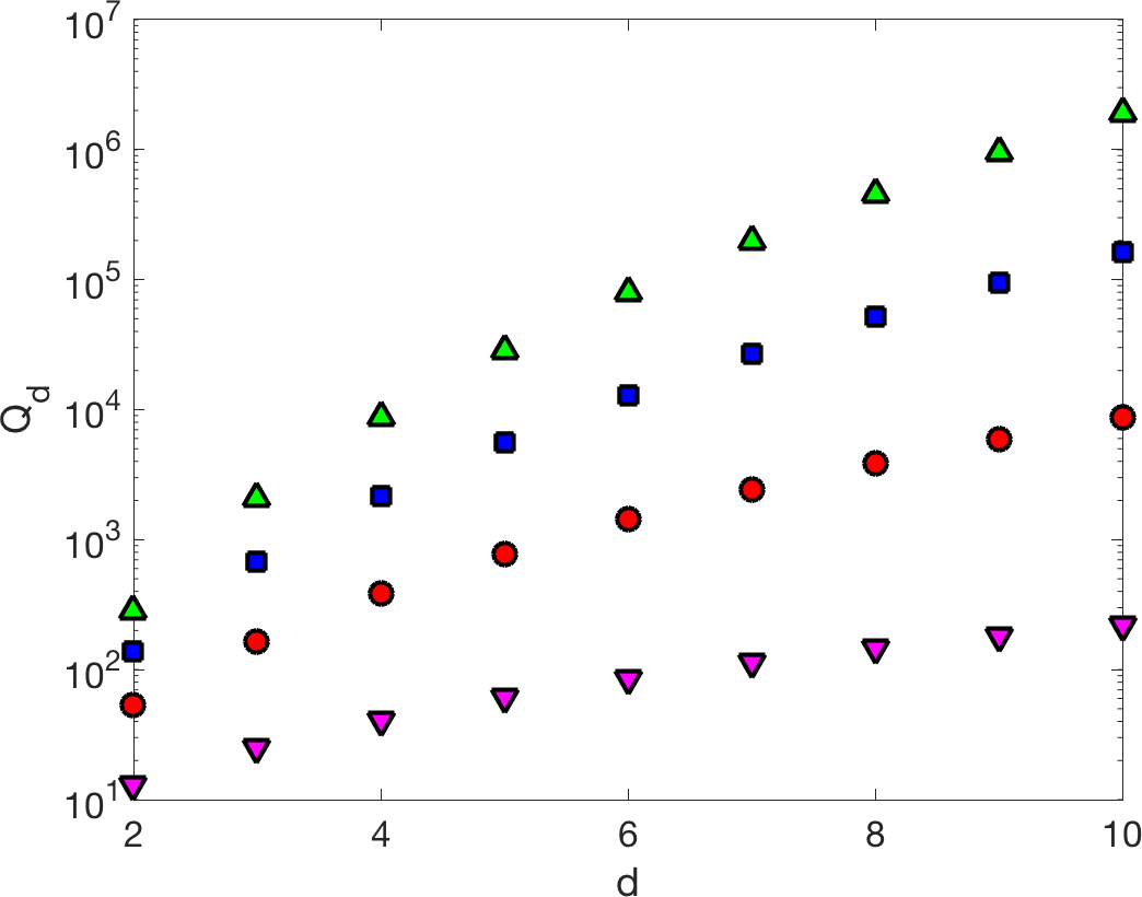
Figure 1: Plot showing the number of sparse grid points $Q_{d}$ against dimension $d$ for $N=1$ ($\triangledown$), $N=3$ ($\bigcirc$), $N=5$ ($\square$) and $N=7$ ($\triangle$).

The accuracy of the gPC representation in Section 2 depends on taking $d$ sufficiently large that $a(\boldsymbol{x},\omega)$ is well approximated by the truncated Karhunen-Loeve expansion (2.1). On the other hand, reducing the computational cost of the gPC method requires keeping $d$ sufficiently small such that the number of sparse grid quadrature points, needed to evaluate the coefficients in (2.4), is manageable. In Figure 1 we demonstrate the rapid growth in the number of sparse grid points required to compute the gPC approximation (2.3) as the stochastic dimension $d$ increases for polynomials with maximum degree $N=1,3,5,7$.

In this section we briefly review a recently proposed domain decomposition method in conjunction with coarse stochastic solution [13] that provides optimal low dimensional subspaces of $\mathbb{R}^{d}$ on which to approximate the solution $u(\boldsymbol{x},\omega)$. This facilitates the construction of a new gPC approximation with lower stochastic dimension than $d$, and hence significantly fewer stochastic quadrature points are required (see Figure 1).

The key to the domain decomposition method is to observe that the quantity of interest $u(\boldsymbol{x},\omega)$ can itself be viewed as a random field on $D$ with covariance

$$C_{u}(\boldsymbol{x},\boldsymbol{y})=\mathbb{E}\bigg{[}\Big{(}u(\boldsymbol{x},\cdot)-\mathbb{E}[u(\boldsymbol{x},\cdot)]\Big{)}\Big{(}u(\boldsymbol{y},\cdot)-\mathbb{E}[u(\boldsymbol{y},\cdot)]\Big{)}\bigg{]},\qquad\boldsymbol{x},\boldsymbol{y}\in D.$$ (4.1)

It follows that the Hilbert-Karhunen-Loeve expansion can be used to find a low stochastic-dimension approximation to $u(\boldsymbol{x},\omega)$, similar to the expansion of $a(\boldsymbol{x},\omega)$ in Section 1. Motivated by the fact that random fields typically have lower rank approximation on smaller domains [13], we decompose the spatial domain $D$ into subdomains $D_{1},\dots,D_{S}$ satisfying

$$D=\bigcup_{s=1}^{S}D_{s},\qquad D_{s}\cap D_{s^{\prime}}=\emptyset\ \mbox{for $s\neq s^{\prime}$}.$$

On each subdomain we use the readily computable approximation to the covariance in (4.1)

$$C^{s}_{u_{1}}(\boldsymbol{x},\boldsymbol{y})=\mathbb{E}\bigg{[}\Big{(}u_{1}(\boldsymbol{x},\cdot)-\mathbb{E}[u_{1}(\boldsymbol{x},\cdot)]\Big{)}\Big{(}u_{1}(\boldsymbol{y},\cdot)-\mathbb{E}[u_{1}(\boldsymbol{y},\cdot)]\Big{)}\bigg{]},\qquad\boldsymbol{x},\boldsymbol{y}\in D_{s},$$ (4.2)

where the coarse stochastic solution $u_{1}(\boldsymbol{x},\boldsymbol{\xi})$ is the degree 1 gPC approximation given by (2.3). Using the orthonormality of the tensor product polynomials (2.7) and the expansion (2.3) we have

$$C^{s}_{u_{1}}(\boldsymbol{x},\boldsymbol{y})=\sum_{|\boldsymbol{n}|=1}u_{\boldsymbol{n}}(\boldsymbol{x})u_{\boldsymbol{n}}(\boldsymbol{y}),\qquad\boldsymbol{x},\boldsymbol{y}\in D_{s}.$$ (4.3)

For polynomial degree $N=1$ the number of sparse grid points required is very low (see Figure 1) so that computing the gPC approximation $u_{1}(\boldsymbol{x},\boldsymbol{\xi})$ is computationally inexpensive, even when $\boldsymbol{\xi}$ has the full $d$ dimensions.

Using (4.3), the truncated Karhunen-Loeve expansion for $u_{1}(\boldsymbol{x},\boldsymbol{\xi})$ is

$$u_{1}(\boldsymbol{x},\boldsymbol{\xi}(\omega))\approx u_{\boldsymbol{0}}(\boldsymbol{x})+\sum_{i=1}^{d}\sqrt{\mu^{s}_{i}}b^{s}_{i}(\boldsymbol{x})\eta^{s}_{i}(\omega),$$ (4.4)

where $u_{\boldsymbol{0}}(\boldsymbol{x})$ is the mean of $u_{1}(\boldsymbol{x},\cdot)$ and $\eta^{s}_{1},\dots,\eta^{s}_{d}$ are independent Gaussian random variables with zero mean and unit standard deviation. The eigenpairs $(b^{s}_{i},\mu^{s}_{i})$ satisfy the eigenvalue problem

$$\int_{D}C^{s}_{u_{1}}(\boldsymbol{x},\boldsymbol{y})b^{s}_{i}(\boldsymbol{y})\;ds(\boldsymbol{y})=\mu^{s}_{i}b^{s}_{i}(\boldsymbol{x}),\qquad i=1,\dots,d.$$ (4.5)

In practice, (4.5) can be discretized (see example-specific details in Section 6), leading to an algebraic eigenvalue problem that can be solved efficiently using the QR algorithm. All of the eigenvalues of (4.5) are positive, and we take $\mu_{1}^{s},\dots,\mu_{d}^{s}$ to be the $d$ largest eigenvalues, ordered so that

$$\mu^{s}_{1}\geq\dots\geq\mu^{s}_{d}>0.$$

On the left hand side of (4.4), the random field $u_{1}(\boldsymbol{x},\cdot)$ is represented as a function of $\xi_{1}(\omega),\dots,\xi_{d}(\omega)$. On the right hand side of (4.4), the random field $u_{1}(\boldsymbol{x},\cdot)$ is represented as a function of $\eta^{s}_{1}(\omega),\dots,\eta^{s}_{d}(\omega)$. That is, we have two different parametrizations of $u_{1}(\boldsymbol{x},\cdot)$ with respect to $d$ stochastic variables. These parametrizations are related via the orthogonal linear transformation [13]

$$\eta^{s}_{i}=\sum_{j=1}^{d}a^{s}_{ij}\xi_{j},\qquad i=1,\dots,d,$$ (4.6)

where

$$a^{s}_{ij}=\frac{1}{\sqrt{\mu^{s}_{i}}}\int_{D_{s}}u_{\boldsymbol{e}_{j}}(\boldsymbol{x})b^{s}_{i}(\boldsymbol{x})\;ds(\boldsymbol{x}),$$ (4.7)

and $\boldsymbol{e}_{j}$ is the $j$th Euclidean vector in $\mathbb{R}^{d}$.

The approximation (4.4) is associated with the restricted domain $D_{s}$ on which the variance of $u_{1}(\boldsymbol{x},\cdot)$ is expected to be less than on the full domain $D$. Consequently the eigenvalues $\mu^{s}_{1},\dots,\mu^{s}_{d}$ are expected to decay sufficiently quickly that the number of terms on the right hand side of (4.4) can be reduced without significantly compromising the accuracy of the approximation. This motivates further truncating the Karhunen-Loeve expansion (4.4) to obtain the approximation

$$u_{1}(\boldsymbol{x},\boldsymbol{\xi}(\omega))\approx u_{\boldsymbol{0}}(\boldsymbol{x})+\sum_{i=1}^{r}\sqrt{\mu^{s}_{i}}b^{s}_{i}(\boldsymbol{x})\eta^{s}_{i}(\omega),$$ (4.8)

with $r<d$. The expansion (4.8) provides an approximation of the random field $u_{1}(\boldsymbol{x},\cdot)$ for $\boldsymbol{x}\in D_{s}$ using a reduced dimension stochastic space.

The advantage of (4.8) is in identifying a reduced dimension stochastic space appropriate for constructing a local approximation to $u(\boldsymbol{x},\cdot)$ for $\boldsymbol{x}\in D_{s}$. In particular, writing $\boldsymbol{\eta}^{s}=(\eta^{s}_{1},\dots,\eta^{s}_{r})$ we have

$$u(\boldsymbol{x},\boldsymbol{\xi}(\omega))\approx u^{s}(\boldsymbol{x},\boldsymbol{\eta}^{s}(\omega)),\qquad\boldsymbol{x}\in D_{s},$$ (4.9)

where $u^{s}(\boldsymbol{x},\boldsymbol{\eta}^{s})=u(\boldsymbol{x},A^{s}\boldsymbol{\eta}^{s})$ and

$$\boldsymbol{\eta}^{s}=(A^{s})^{T}\boldsymbol{\xi}.$$ (4.10)

Here $A^{s}$ is the $d\times r$ matrix with entries

$$A^{s}_{ij}=a^{s}_{ij},\qquad i=1,\dots,d,\ j=1,\dots,r,$$

where $a^{s}_{ij}$ is given by (4.7).

Following the details in Section 2 we approximate $u^{s}(\boldsymbol{x},\boldsymbol{\eta}^{s})$ by a truncated gPC approximation

$$u^{s}_{N_{s}}(\boldsymbol{x},\boldsymbol{\eta}^{s})=\sum_{|\boldsymbol{n}|=0}^{N_{s}}u^{s}_{\boldsymbol{n}}(\boldsymbol{x})\psi_{\boldsymbol{n}}(\boldsymbol{\eta}^{s})$$ (4.11)

where

$$u^{s}_{\boldsymbol{n}}(\boldsymbol{x})=\langle u^{s}(\boldsymbol{x},\boldsymbol{\eta}^{s}),\psi_{\boldsymbol{n}}\rangle=\langle u(\boldsymbol{x},A^{s}\boldsymbol{\eta}^{s}),\psi_{\boldsymbol{n}}\rangle.$$ (4.12)

In practice the inner product in (4.12) is computed using the sparse grid quadrature rule

$$\int_{\mathbb{R}^{r}}f(\boldsymbol{\xi})\;w(\boldsymbol{\eta})\;ds(\boldsymbol{\eta})\approx\sum_{q=1}^{Q_{r}}w^{r,Q_{r}}_{q}f(\boldsymbol{\sigma}^{r,Q_{r}}_{q}).$$ (4.13)

The gPC approximation (4.11) is cheaper to compute than (2.3) because it has lower stochastic dimension and hence the sparse grid quadrature rule has fewer points (see Figure 1). In particular, $Q_{r}<Q_{d}$.

Using the gPC approximation (4.11) we compute approximations to the mean and variance,

$$\mathbb{E}[u(\boldsymbol{x},\cdot)]\approx u_{\boldsymbol{0}}^{s},\qquad\mathbb{V}[u(\boldsymbol{x},\cdot)]\approx\sum_{|\boldsymbol{n}|=1}^{N_{s}}|u_{\boldsymbol{n}}^{s}(\boldsymbol{x})|^{2},\qquad\boldsymbol{x}\in D_{s}.$$ (4.14)

5 Epistemic uncertainty for the Domain Decomposition method

As in Section 3, we again let the standard deviation of the random field $a_{\tau}$ be $\tau\sigma_{\mathrm{max}}$ for some parameter $\tau>0$. Then using the Karhunen-Loeve expansion (3.2) for $a_{\tau}$, the change of variables $\boldsymbol{\theta}^{s}=\tau\boldsymbol{\eta}^{s}$, and the transformation (4.10), we can approximate

$$u^{\tau}(\boldsymbol{x},\boldsymbol{\zeta})\approx u^{\tau,s}(\boldsymbol{x},\boldsymbol{\theta}^{s}),\qquad\boldsymbol{x}\in D_{s},$$ (5.1)

where $u^{\tau,s}(\boldsymbol{x},\boldsymbol{\theta}^{s})=u^{\tau}(\boldsymbol{x},A^{s}\boldsymbol{\theta}^{s})$, with

$$\boldsymbol{\theta}^{s}=(A^{s})^{T}\boldsymbol{\zeta},$$ (5.2)

and $A^{s}$ is the matrix given in Section 4.

Similar to Section 2, we seek an approximation to the local quantity of interest $u^{\tau,s}(\boldsymbol{x},\boldsymbol{\theta}^{s})$ for $\boldsymbol{x}\in D_{s}$ of the form

$$u^{\tau,s}_{N}(\boldsymbol{x},\boldsymbol{\theta}^{s})=\sum_{|\boldsymbol{n}|=0}^{N_{s}}u^{\tau,s}_{\boldsymbol{n}}(\boldsymbol{x})\psi^{\tau}_{\boldsymbol{n}}(\boldsymbol{\theta}^{s})$$ (5.3)

where $u^{\tau,s}_{\boldsymbol{n}}(\boldsymbol{x})$ are the gPC coefficients, given by

$$u^{\tau,s}_{\boldsymbol{n}}(\boldsymbol{x})=\langle u^{\tau,s}(\boldsymbol{x},\cdot),\psi^{\tau}_{\boldsymbol{n}}\rangle_{\tau}.$$ (5.4)

Surrogate gPC approximation

As in Section 3, in the remainder of this section we suppose that the local gPC approximation $u^{s}(\boldsymbol{x},\boldsymbol{\eta})$ has been computed. Following the details in Section 3, it is appropriate to use $u^{s}_{N}(\boldsymbol{x},\boldsymbol{\theta}^{s})$ as a surrogate for $u^{\tau,s}_{N}(\boldsymbol{x},\boldsymbol{\theta}^{s})$. Using this surrogate in (5.4) gives surrogate gPC coefficients

$$\widehat{u}^{\tau,s}_{\boldsymbol{n}}(\boldsymbol{x})=\langle u^{s}_{N}(\boldsymbol{x},\cdot),\psi^{\tau}_{\boldsymbol{n}}\rangle_{\tau}.$$ (5.5)

Similar to (3.8) in Section 3 we have

$$\widehat{u}^{\tau,s}_{\boldsymbol{n}}(\boldsymbol{x})=\sum_{|\boldsymbol{m}|=1}^{N}T^{r,\tau}_{\boldsymbol{n},\boldsymbol{m}}u^{s}_{\boldsymbol{m}},$$ (5.6)

where $T^{r,\tau}$ is given by (3.9).

Using the details above, our surrogate approximation to $u^{\tau,s}(\boldsymbol{x},\boldsymbol{\theta}^{s})$ for $\boldsymbol{x}\in D_{s}$ is

$$\widehat{u}^{s,\tau}_{N}(\boldsymbol{x},\boldsymbol{\theta}^{s})=\sum_{|\boldsymbol{n}|=0}^{N}\widehat{u}^{s,\tau}_{\boldsymbol{n}}(\boldsymbol{x})\psi^{\tau}_{\boldsymbol{n}}(\boldsymbol{\theta}^{s})$$ (5.7)

and the surrogate coefficients $\widehat{u}^{s,\tau}_{\boldsymbol{n}}(\boldsymbol{x})$ are computed from the coefficients $u^{s}_{\boldsymbol{n}}(\boldsymbol{x})$ using the matrix-vector product (5.6). As in Section 3, the surrogate gPC coefficients are computationally inexpensive to compute and, in particular, the surrogate coefficients can be obtained without computing further solutions of the PDE (1.1). The mean and variance of the surrogate gPC polynomial,

$$\mathbb{E}_{\tau}[\widehat{u}^{s,\tau}_{N}(\boldsymbol{x},\cdot)]=\widehat{u}^{s,\tau}_{\boldsymbol{0}},\qquad\mathbb{V}_{\tau}[\widehat{u}^{s,\tau}_{N}(\boldsymbol{x},\cdot)]=\sum_{|\boldsymbol{n}|=1}^{N}|\widehat{u}_{\boldsymbol{n}}^{s,\tau}(\boldsymbol{x})|^{2}$$ (5.8)

also provide computationally cheap approximations to the mean and variance of $u^{\tau,s}(\boldsymbol{x},\boldsymbol{\theta}^{s})$ for $\boldsymbol{x}\in D_{s}$.

6 Numerical Results

In this section we demonstrate the efficiency of our surrogate based EUQ algorithm for two distinct stochastic models. The first model describes wave propagation in an unbounded medium, exterior to an uncertain configuration, and the second model is a widely investigated diffusion process with uncertain permeability field. We investigate our EUQ algorithm with and without applying the domain decomposition framework, and show that the latter is essential for solving a $100$-dimensional model, arising due to slow decay of eigenvalues.

A stochastic wave propagation model in unbounded region

We consider multiple scattering of a time harmonic transverse electric (TE) polarized electromagnetic wave by a configuration of $M=25$ parallel perfectly conducting cylinders whose positions are described by a random field. For this uncertain configuration model, we let $K(\omega)\subseteq\mathbb{R}^{2}$ denote the cross section of the cylinders. Then

$$K(\omega)=\cup_{i=1}^{M}K_{i}(\omega),$$ (6.1)

where the unit disk $K_{i}(\omega)$ is the cross section of the $i$th cylinder. In our model $K_{i}(\omega)$ has center $\boldsymbol{x}_{i}(\omega)=\boldsymbol{x}_{i}+a(\boldsymbol{x}_{i},\omega)\boldsymbol{d}$, where $\boldsymbol{d}=(1,1)^{T}/\sqrt{2}$ is the translation direction and $a(\boldsymbol{x},\omega)$ is a normal random field satisfying (1.2) on $E=\mathbb{R}^{2}$ with variance $\sigma_{\mathrm{max}}=0.05$ and $L=\mathop{\mathrm{diag}}(1/l,1/l)$. Here, $l=10$ is the correlation length and the constant $\boldsymbol{x}_{i}$ is the mean of the centre $\boldsymbol{x}_{i}(\omega)$ of the $i$th scatterer. In our experiments $\boldsymbol{x}_{i}$ for $i=1,\dots,M$ are chosen at random in the square $[0,10]\times[0,10]$. A sample of $K(\omega)$ is visualized in Figure 2.

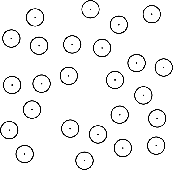
Figure 2: Visualization of a sample of $K(\omega)$ for a configuration of 25 cylinders.

The configuration $K(\omega)$ is illuminated by an incident plane wave modelled by the scalar field

$$v^{\mathrm{inc}}(\boldsymbol{x})=e^{ikx_{2}},$$

where $k=c/\omega$ is the wavenumber and $c$ is the speed of light. The resulting scattered field is modelled by scalar field $v(\boldsymbol{x};\omega)$ that satisfies the two-dimensional Helmholtz equation

$$\triangle v(\boldsymbol{x};\omega)+k^{2}v(\boldsymbol{x};\omega)=0,\qquad\boldsymbol{x}\in\mathbb{R}^{2}\setminus\overline{K(\omega)},$$ (6.2)

together with the perfect conductor boundary condition

$$v(\boldsymbol{x};\omega)=-v^{\mathrm{inc}}(\boldsymbol{x}),\qquad\boldsymbol{x}\in\partial K(\omega),$$ (6.3)

where $\partial K(\omega)$ denotes the boundary of $K(\omega)$, and the radiation condition

$$\lim_{r\rightarrow\infty}\sqrt{r}\left(\frac{\partial v}{\partial r}-ikv\right)=0,\qquad r=|\boldsymbol{x}|,$$ (6.4)

uniformly for all directions $\theta$, where we have used two dimensional polar coordinates $\boldsymbol{x}=(r\cos\theta,r\sin\theta)$. A consequence of (6.4) is that the scattered field can be written

$$v(r,\theta,\omega)\approx\frac{e^{ikr}}{\sqrt{r}}v_{\infty}(\theta;\omega),\qquad\theta\in D,$$ (6.5)

where $D=[0,2\pi)\subseteq\mathbb{R}$. The function $v_{\infty}(\theta,\omega)$ is known as the far field of $v$ and is used to compute the radar cross section

$$u(\theta,\omega)=|v_{\infty}(\theta;\omega)|^{2},$$ (6.6)

which is typically the quantity of interest in applications. The radar cross section of the configuration in Figure 2 is visualized in Figure 3.

We discretize the eigenvalue problem (2.2) using a Monte Carlo quadrature scheme with equal weights and nodes at the mean centers $\boldsymbol{x}_{i}$ for $i=1,\dots,25$ of the cylinders. The decay of the eigenvalues of $C(\boldsymbol{x},\boldsymbol{y})$ is shown in Figure 4 and we choose truncation parameter $d=10$ leading to a Karhunen-Loeve approximation (2.1) of $a(\boldsymbol{x},\omega)$ with respect to the random variable $\boldsymbol{\xi}$ with stochastic dimension $d=10$.

In Table 1 we present the relative error maximum norm of the approximation (2.8) to the mean computed using the gPC scheme in Section 2. The gPC coefficients are computed using (2.4) and the quadrature scheme (2.9). For each fixed $\boldsymbol{\xi}$ we compute $u(\boldsymbol{x},\boldsymbol{\xi})$ in (2.4) by efficiently solving the associated deterministic wave scattering PDE (6.2)–(6.4) and computing the far field (6.5) using the Matlab package MieSolver [14], which is based on the Mie series [15, 16] (see also the books [17, 18, 19]). In practice we compute a discrete approximation to the maximum norm using 1000 equally spaced points in $[0,2\pi]$,

$$x_{i}=2\pi\frac{i-1}{1000},\qquad i=1,\dots,1000.$$ (6.7)

Next we decompose the domain $D=[0,2\pi]$ into $S$ subdomains

$$D_{s}=[2\pi(s-1)/S,2\pi s/S),\qquad s=1,\dots,S.$$

On each domain $D_{s}$ we compute the gPC approximation $u_{1}(\boldsymbol{x},\boldsymbol{\xi})$ as described above. We discretize the eigenvalue problem (4.5) using an equal weight quadrature scheme with nodes at the points (6.7). The decay of the eigenvalues of $C^{s}_{u_{1}}(\boldsymbol{x},\boldsymbol{y})$ for $S=5$ subdomains is shown in Figure 4. The figure shows that the eigenvalues of $C^{s}_{u_{1}}(\boldsymbol{x},\boldsymbol{y})$ decay faster than the eigenvalues of $C(\boldsymbol{x},\boldsymbol{y})$ so that it is appropriate to apply the dimension reduction approach in Section 4.

In Table 2 we tabulate the relative error maximum norm of the approximation (4.14) to the mean computed using the domain decomposition scheme in Section 4. We demonstrate that the domain decomposition technique is able to produce an approximation of comparable quality to the $d=10$ gPC scheme using only $r=5$ dimensions. The $d=10$ gPC scheme requires evaluation of the PDE model for 162 025 values of the stochastic parameter $\boldsymbol{\xi}$, whereas the domain decomposition scheme with $r=5$ requires evaluation of the PDE at only 5593 values of the stochastic parameter $\boldsymbol{\eta}$ for each subdomain. Thus the domain decomposition method is significantly cheaper. In Figures 5 and 6 we plot the mean and standard deviations of the cross sections (6.6) computed using the gPC method (2.8) with $d=10$ and the domain decomposition method (4.14) with $r=5$.

In Table 3 we demonstrate the accuracy of our approximations by comparing with reference solutions obtained using Monte Carlo applied directly for random fields $a(\boldsymbol{x},\omega)$ with covariance given by (1.2) with $\sigma$ replaced by $\tau\sigma_{\mathrm{max}}$. In Tables 5–6 we demonstrate the accuracy of the epistemic post-processing algorithm for the wave propagation problem, when compared to the associated aleatoric gPC model, with and without domain decomposition.

In Figure 7 we visualize the approximations to the mean and standard deviation of the backscattered cross section as a function of $\tau$, where $\tau\sigma_{\mathrm{max}}$ is the standard deviation of the input random field $a(\boldsymbol{x},\omega)$. The backscattered cross section approximations are computed using (5.8) with backscattering direction $\boldsymbol{x}=3\pi/2$.

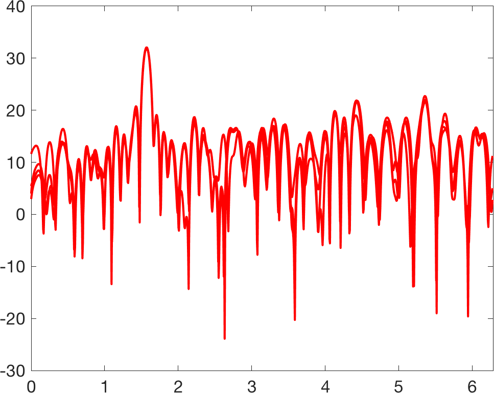
Figure 3: Visualization of the radar cross section of the configuration in Figure 2 in decibels $10\log_{10}2\pi u(\theta;\omega)$.

$d$	rel. error
4	2.55e-03
6	1.00e-03
8	3.70e-04
10	1.60e-04

Table 1: Maximum norm relative error in the approximation to the mean $u(\boldsymbol{x},\omega)$ computed using the gPC method with stochastic dimensions $r=4,6,8,10$. The reference solution is computed using 1 048 576 Monte Carlo simulations.

$d$	rel. error
4	1.20e-03
5	6.62e-04
6	4.15e-04

Table 2: Maximum norm error of the approximation to the mean $u(\boldsymbol{x},\omega)$ computed using the domain decomposition method with $S=5$ subdomains and stochastic dimensions $r=4,5,6$. The reference solution is computed using 1 048 576 Monte Carlo simulations.

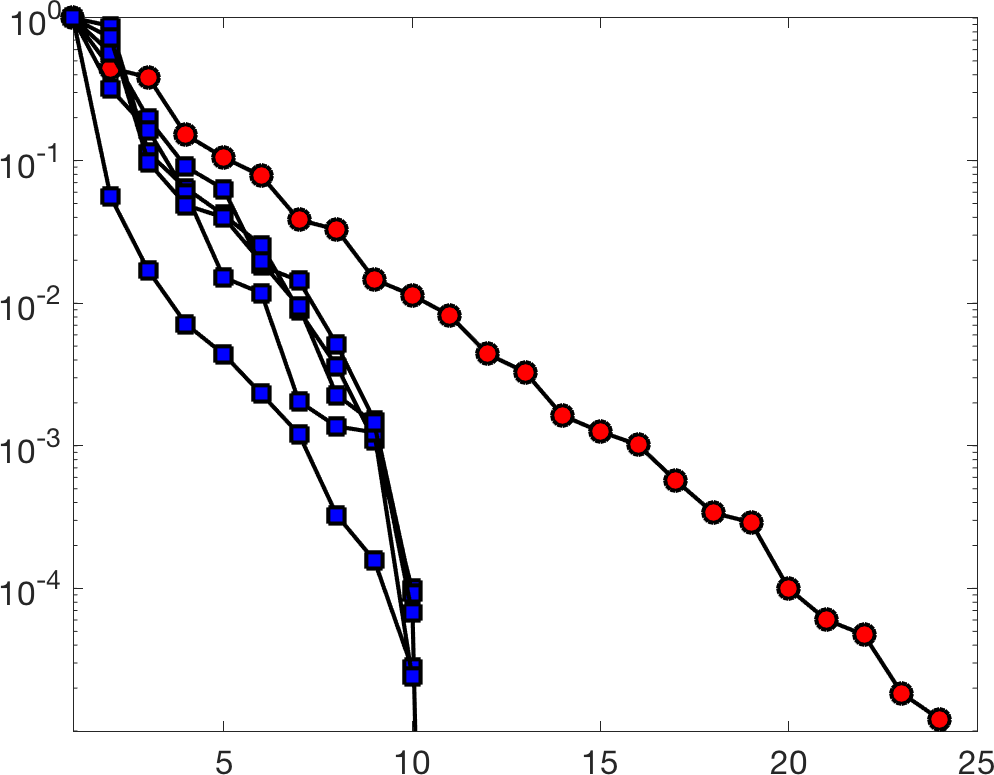
Figure 4: Decay of the eigenvalues of the covariance function $C(\boldsymbol{x},\boldsymbol{y})$ ($\bigcirc$) and the covariance functions $C^{s}_{u_{1}}(\boldsymbol{x},\boldsymbol{y})$ ($\square$) for $s=1,\dots,S$ with stochastic dimension $d=10$ and $S=5$ subdomains.

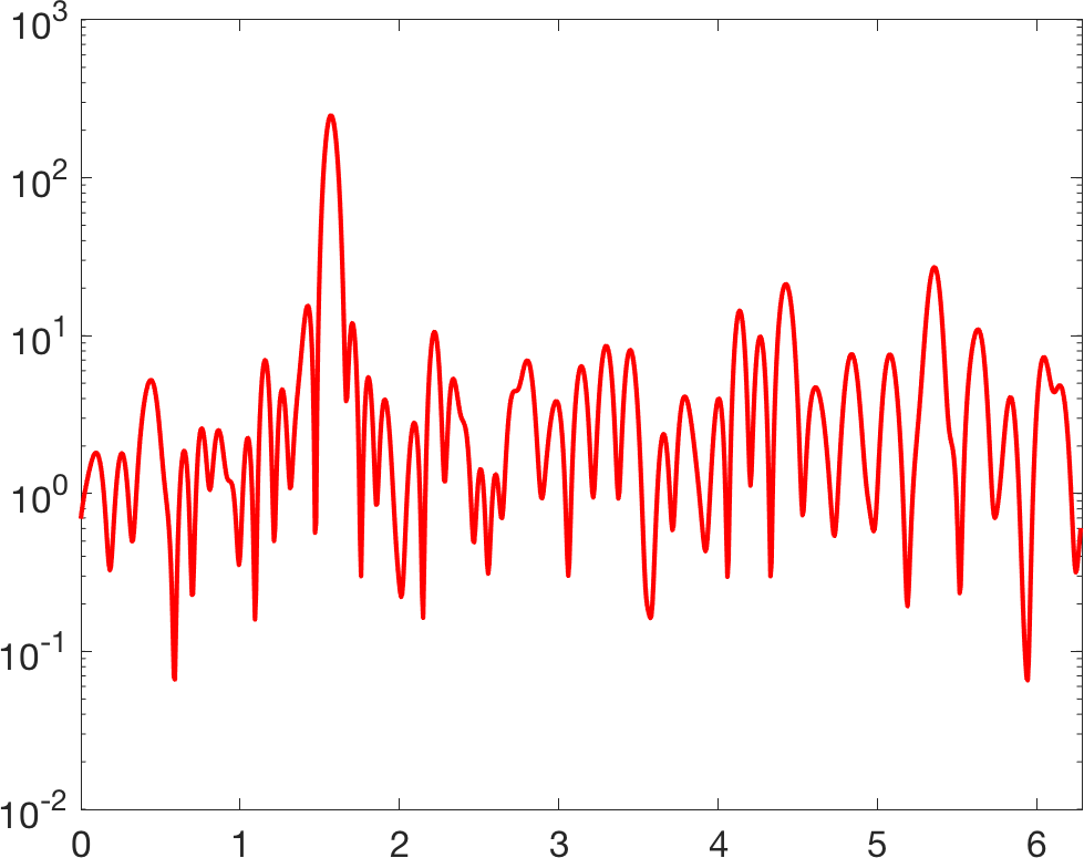
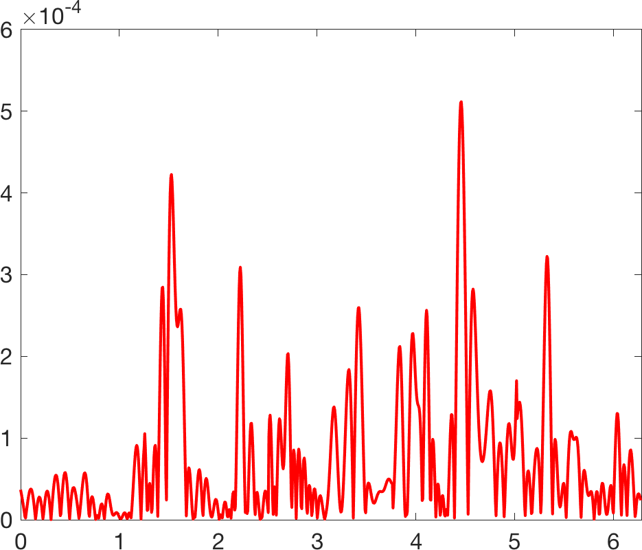
(a) Mean of $u_{N}(\boldsymbol{x},\boldsymbol{\xi})$ for $d=10$	(b) Mean of $u_{N}^{s}(\boldsymbol{x},\boldsymbol{\zeta})$ for $r=5$	(c) relative difference

Figure 5: Approximations to the mean of $u(\boldsymbol{x},\omega)$ obtained without domain decomposition (a) and with domain decomposition (b) using $S=5$ subdomains.

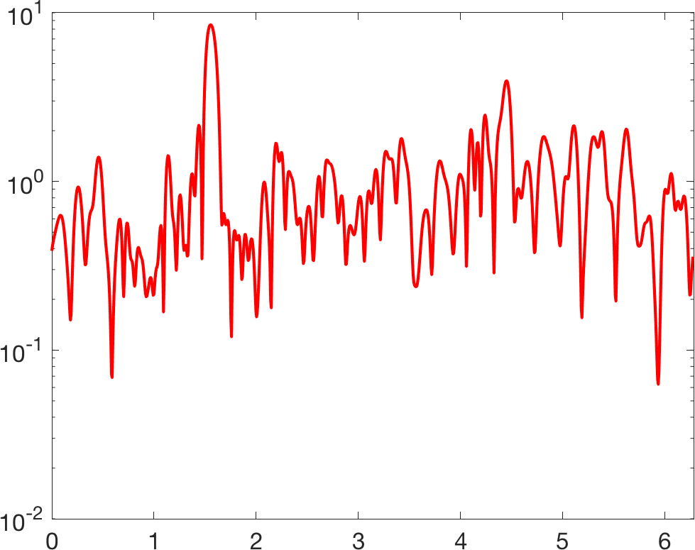
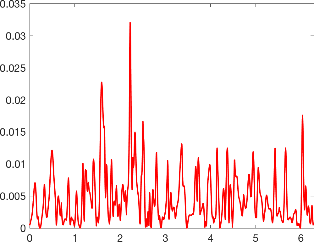
(a) Standard deviation of $u_{N}(\boldsymbol{x},\boldsymbol{\xi})$ for $d=10$	(b) Standard deviation of $u_{N}^{s}(\boldsymbol{x},\boldsymbol{\zeta})$ for $r=5$	(c) relative difference

Figure 6: Approximations to the standard deviation of $u(\boldsymbol{x},\omega)$ obtained without domain decomposition (a) and with domain decomposition (b) using $S=5$ subdomains.

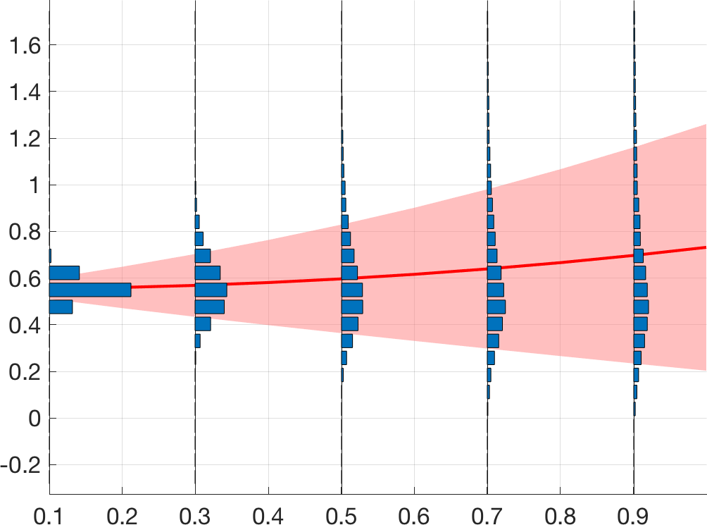
Figure 7: Visualization of the mean (solid line) and standard deviation (indicated by shading) of the cross section $u(\boldsymbol{x},\omega)$ plotted against $\tau$. The random field $a(\boldsymbol{x},\omega)$ has standard deviation $\tau\sigma_{\mathrm{max}}$ for $0<\tau<1$. The mean and standard deviation are computed using the efficient method in Section 5. Samples with 10 000 Monte Carlo samples are visualized in the histograms.

$\tau$	rel. error
0.2	2.22e-03
0.4	1.80e-03
0.6	1.10e-03
0.8	3.59e-04
1.0	6.62e-04

Table 3: Maximum norm relative error of the approximation to the mean computed using the domain decomposition method in Section 5 for random field with standard deviation $\tau\sigma_{\mathrm{max}}$. The reference solution is computed using 1 048 576 Monte Carlo simulations.

$\tau$	rel. error
0.2	1.71e-02
0.4	1.33e-02
0.6	8.06e-03
0.8	2.81e-03
1.0	1.82e-04

Table 4: Maximum norm relative error of the approximation to the mean computed using the method in Section 3 for random field with standard deviation $\tau\sigma_{\mathrm{max}}$. The reference solution is computed using 1 048 576 Monte Carlo simulations.

$\tau$	max. rel. mean error	max. rel. variance error
0.9	9.9416e-04	3.7682e-02
0.8	2.9073e-03	1.0801e-01
0.7	5.3900e-03	1.9246e-01
0.6	8.1333e-03	2.7751e-01
0.5	1.0871e-02	3.5289e-01
0.4	1.3383e-02	4.1282e-01
0.3	1.5497e-02	4.5643e-01
0.2	1.7087e-02	4.8519e-01
0.1	1.8072e-02	5.0129e-01

Table 5: Ten-dimensional stochastic diffusion model: Maximum norm relative error of the approximate mean and variance computed using the gPC approach and the post-processed surrogate method in Section 3.

$\tau$	max. rel. mean error	max. rel. variance error
0.9	2.4060e-04	6.4024e-03
0.8	5.5901e-04	1.7486e-02
0.7	9.1775e-04	3.5164e-02
0.6	1.2785e-03	5.6954e-02
0.5	1.6084e-03	8.0734e-02
0.4	1.8847e-03	1.0409e-01
0.3	2.0956e-03	1.2477e-01
0.2	2.2395e-03	1.4090e-01
0.1	2.3216e-03	1.5108e-01

Table 6: Ten-dimensional stochastic diffusion model: Maximum norm relative error of the approximate mean and variance computed using the domain decomposition approach and the post-processed surrogate method in Section 5.

A stochastic diffusion model

We consider the EUQ counterpart of the stochastic diffusion example investigated in [13]. The large, but bounded, spatial domain of the model is $E=[0,240]\times[0,60]$. For $\boldsymbol{x}=(x_{1},x_{2})\in E$, stochasticity in the diffusion model with a mixed (Dirichlet and Neumann) boundary condition (on vertical and horizontal boundaries of $E$), is induced by a log-normal field:

$$-\nabla\cdot\left[\exp(a(\boldsymbol{x},\omega))\nabla u(\boldsymbol{x},\omega)\right] =f(\boldsymbol{x})\;\;\rm{in}~{}E\times\Omega,$$

$$u(\boldsymbol{x},\omega)=50\;\;\text{on}~{}x_{1}=0,\qquad \;\;u(\boldsymbol{x},\omega)=25\;\;\text{on}~{}x_{1}=240,$$

$$\frac{\partial}{\partial\boldsymbol{n}}u(\boldsymbol{x},\omega)=0\;\;\text{on}~{}x_{2}=0,\qquad \frac{\partial}{\partial\boldsymbol{n}}u(\boldsymbol{x},\omega)=0\;\;\text{on}~{}x_{2}=60,$$ (6.8)

where $\boldsymbol{n}(\boldsymbol{x})$ denotes the unit outward normal to $E$ at $\boldsymbol{x}$ and the discontinuous function $f$ is such that the sink value of $f$ at the center of the domain $E$ is $-1$, and $f$ is zero elsewhere. For this model, the QoI is the solution $u$ of (6) and hence $D=E$. As in [13], we choose $L=\mathop{\mathrm{diag}}(1/24,1/20)$, and the mean and maximum standard deviation of $\exp(a)$ to be 5.0 and 2.5 respectively. Hence the mean and maximum standard deviation of the normal random field $a$ are respectively

$$a_{0}(x)=\ln\left(\frac{5}{\sqrt{1+(\frac{2.5}{5})^{2}}}\right)=\ln(5/\sqrt{1.25});\qquad\sigma_{\mathrm{max}}=\sqrt{\ln(1.25)}.$$

We demonstrate the accuracy of the post-processed surrogate solutions of the above model with standard deviations $\tau\sigma_{\mathrm{max}}$, for $0<\tau<1$, obtained using the gPC solution of the model with standard deviation $\sigma_{\mathrm{max}}$.

A $10$-dimensional truncated version of the stochastic model was simulated for fixed standard deviation $\sigma$ using the gPC approximation with $N=3$ and the sparse grid level $N+2$ in [13]. Simulation of reference solutions for this problem requires solving the diffusion PDE $8761$ times, once for each sparse-grid point in the ten-dimensional stochastic space. Using this gPC approximation as the reference solution, it was shown in [13] that a domain decomposition (DD) version of the solution has accuracy $6\times 10^{-5}$ in mean and $7\times 10^{-3}$ in variance. Such an accurate gPC-DD solution was obtained with $S=8$ sub-domains and, for $s=1,\dots,S$, in each sub-domain $D_{s}$ the stochastic dimension was chosen to be $r=3$ and the gPC $N_{s}=N$. Below, we use the same parameters for the EUQ model.

We note that it takes only a few seconds of the CPU time to post-process the $\tau=1$ case reference solution $u_{N}^{\tau}$ to compute the approximation $\widehat{u}_{N}^{\tau}$ to the solution $u_{N}^{\tau}$, for any $0<\tau<1$. In particular, this post-processing does not requires further solves of the PDE model.

For the ten-dimensional stochastic diffusion model, results in Table 7 demonstrate the accuracy in mean and variance of the post-processed surrogate solution $\widehat{u}_{N}^{\tau}$ when compared to the gPC reference solution $u_{N}^{\tau}$, for $\tau=0.1,0.2,\dots,0.9$. The maximum relative error was computed by taking the maximum of the relative errors at the spatial grid points. In Figure 8 we demonstrate the accuracy of the post-processing approach by comparing the probability density estimates for $\widehat{u}_{N}^{\tau}(\boldsymbol{x}^{*},\cdot)$ and $u_{N}^{\tau}(\boldsymbol{x}^{*},\cdot)$ for $\boldsymbol{x}^{*}$ at the centre of $D$. A sample profile in $D$, for the case $\tau=0.1$, of the ten-dimensional mean solution $u_{N}^{\tau}(\cdot,\omega)$, the counterpart post-processed surrogate $\widehat{u}_{N}^{\tau}(\cdot,\omega)$, and the associated relative error, the ten-dimensional EUQ stochastic model are given in Figure 9.

The decay of the eigenvalues of $C$ in $D$ shown in Figure 10 suggests that it may be appropriate to increase the the truncation parameter for the EUQ model to $d=100$. We note that it is not feasible to solve the gPC model in 100-dimensions, with polynomial degree $N=3$, because the PDE would need to be solved for billons of sparse grid realization points. However, using the gPC-DD approach it is feasible. In particular, we first solve for $u_{1}$ in 100-dimensions (with $N=1$, and sparse-grid level $2$), which requires solving the PDE only $201$ times, corresponding to the sparse-grid points in $100$-dimensions. We then use $u_{1}$ in conjunction with the domain-decomposition method with $S=8$ subdomains of $D=(0,240)\times(0,60)$, in a $4\times 2$ grid.

For $s=1,\dots,8$, the eigenvalues of $C_{u_{1}}^{s}$ in $D_{s}$ decay substantially faster, than those of $C$ in $D$. This is demonstrated (for $s=1,2,3$) in Figure 10. Hence, after solving for $u_{1}$ in the 100-dimensional stochastic space we solve the sub-domain problems using $r=3$ stochastic dimensional spaces. The transfer between the sub-domain stochastic variables and the full-domain stochastic variables are computed using the representation in (4.10). For $0<\tau<1$ we carry out the post-processing surrogate approach in Section 5 for each sub-domain model, and compute the corresponding mean and variance efficiently using (5.8).

For the hundred-dimensional stochastic diffusion models, results in Table 8 demonstrate the accuracy in mean and variance of the post-processed surrogate solution $\widehat{u}_{N,DD}^{\tau,8}$ when compared to the gPC-DD reference solution $u_{N,DD}^{\tau,8}$, for $\tau=0.1,0.2,\dots,0.9$. The maximum relative error was computed by taking the maximum of the relative errors at the spatial grid points. In Figure 11 we demonstrate the accuracy of the post-processing approach by comparing the probability density estimates for $\widehat{u}_{N,DD}^{\tau,8}(\boldsymbol{x}^{*},\cdot)$ and ${u}_{N,DD}^{\tau,8}(\boldsymbol{x}^{*},\cdot)$ for $\boldsymbol{x}^{*}$ at the centre of $D$. In Figure 12 we visualize the mean $u_{N,DD}^{\tau,8}(\cdot,\omega)$ and the post-processed surrogate approximation $\widehat{u}_{N,DD}^{\tau,8}(\cdot,\omega)$, for the hundred-dimensional EUQ stochastic model with $\tau=0.1$.

$\tau$	max. rel. mean error	max. rel. variance error
0.9	6.9082e-06	1.6753e-04
0.8	2.4649e-05	3.0185e-04
0.7	4.9307e-05	4.0997e-04
0.6	7.7467e-05	4.9846e-04
0.5	1.0619e-04	5.7096e-04
0.4	1.3302e-04	7.1537e-04
0.3	1.5595e-04	9.0909e-04
0.2	1.7344e-04	1.0596e-03
0.1	1.8436e-04	1.1548e-03

Table 7: Ten-dimensional stochastic diffusion model: Maximum norm relative error of the approximate mean and variance computed using the gPC approach and the post-processed surrogate method.

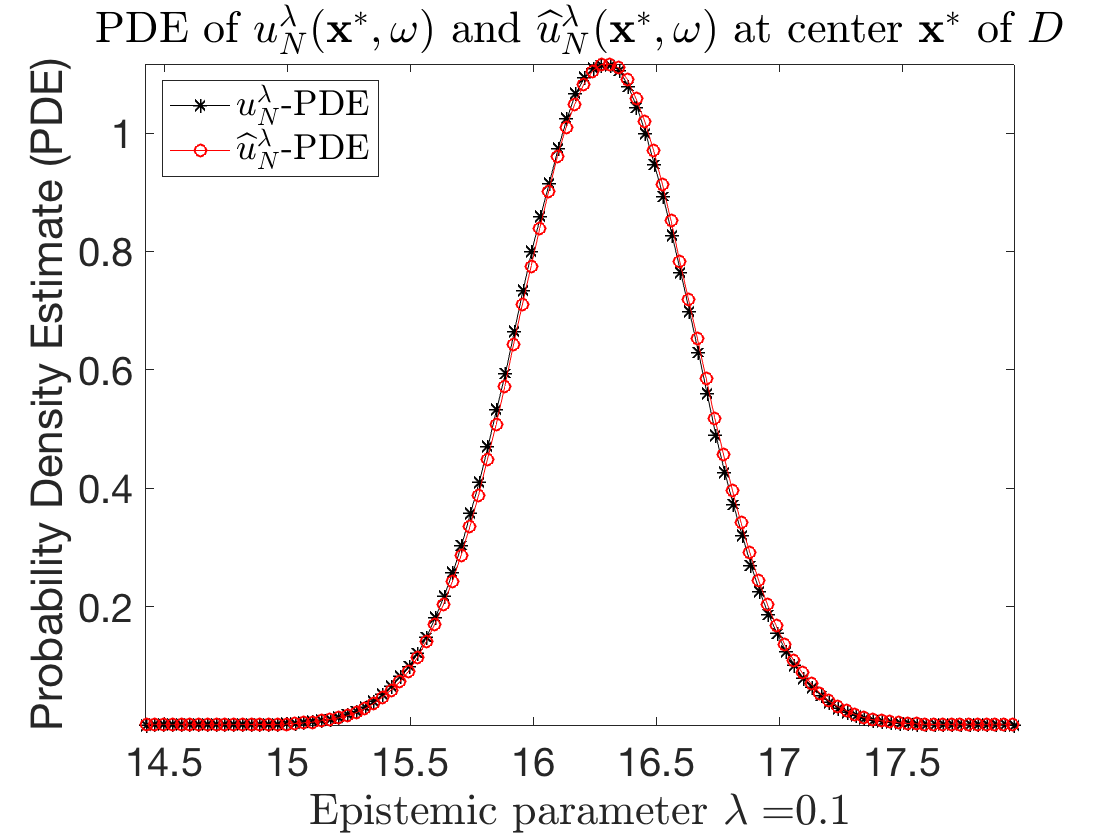
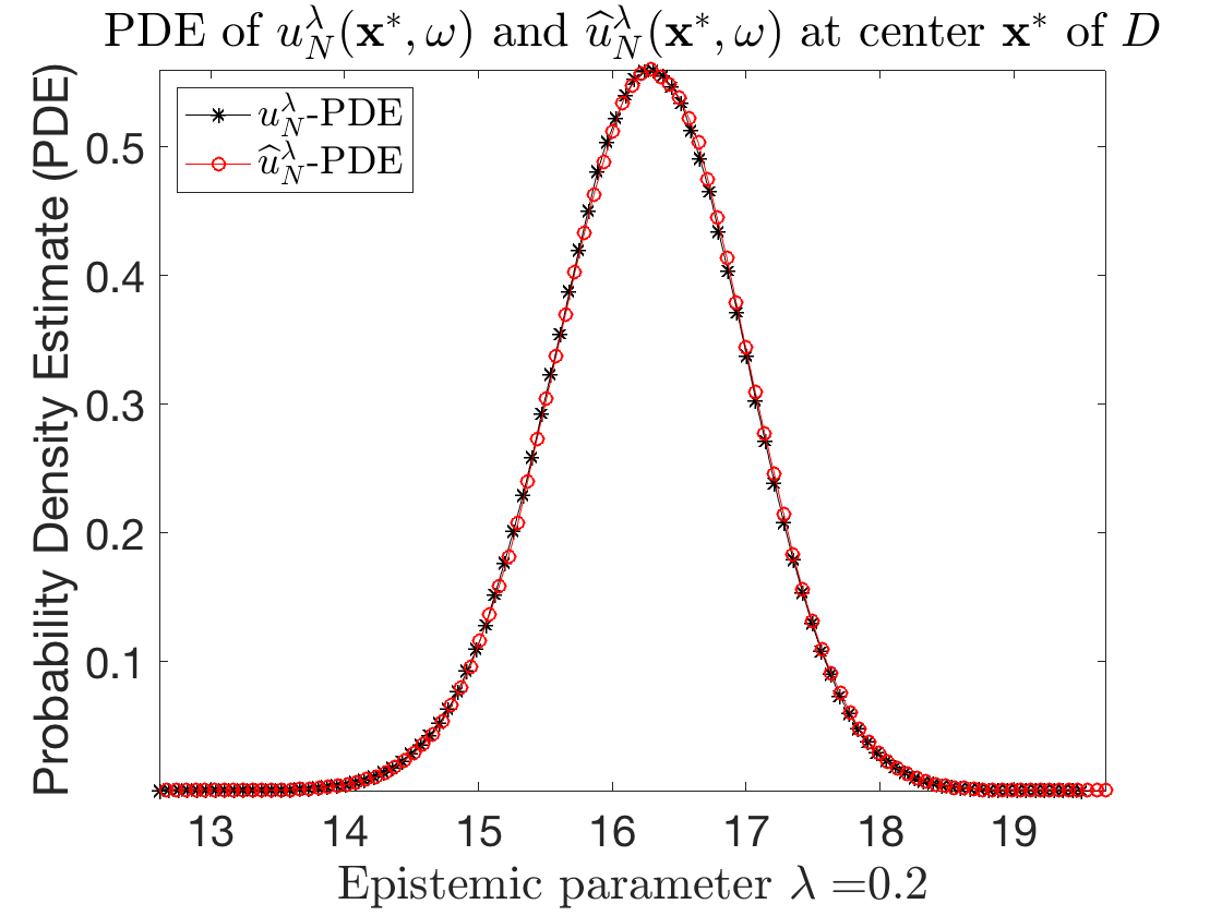
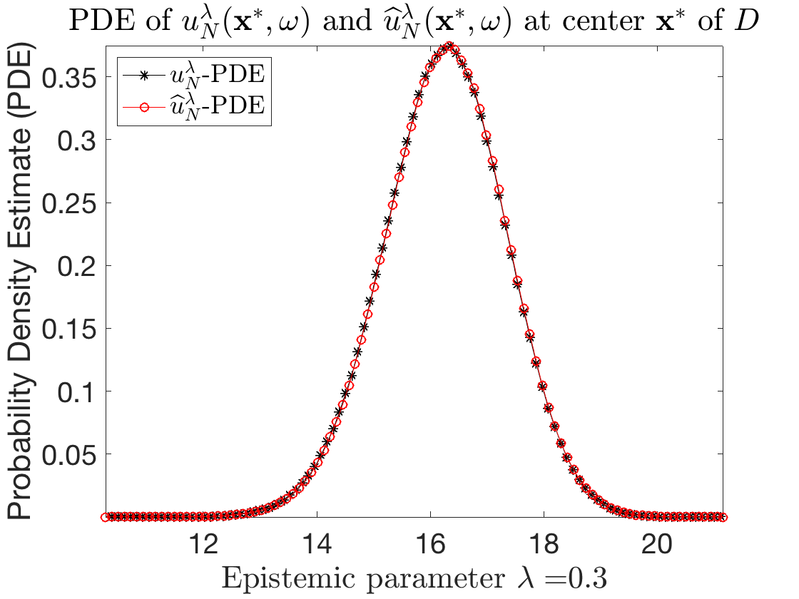
(a) $\tau=0.1$	(b) $\tau=0.2$	(c) $\tau=0.3$
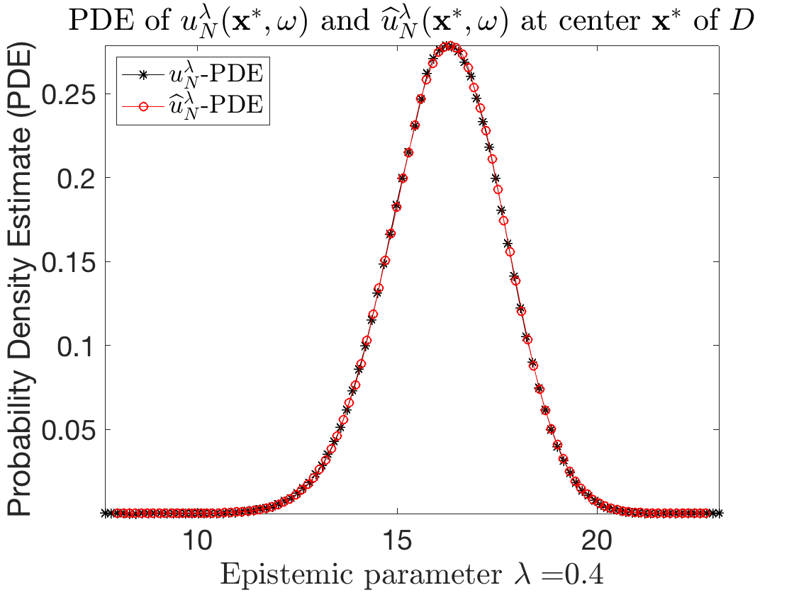
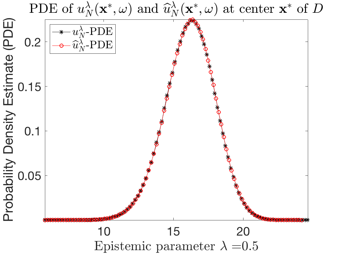
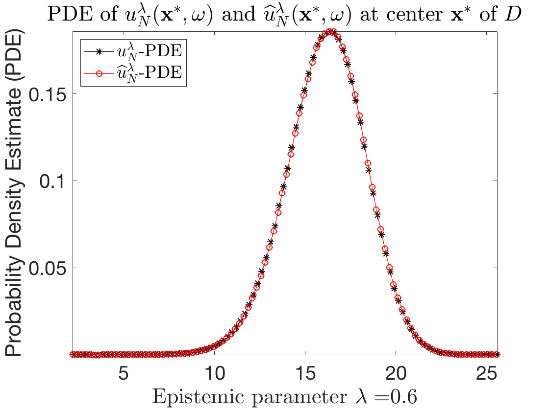
(d) $\tau=0.4$	(e) $\tau=0.5$	(f) $\tau=0.6$
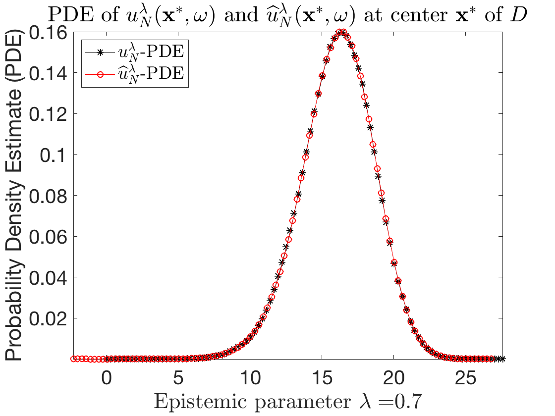
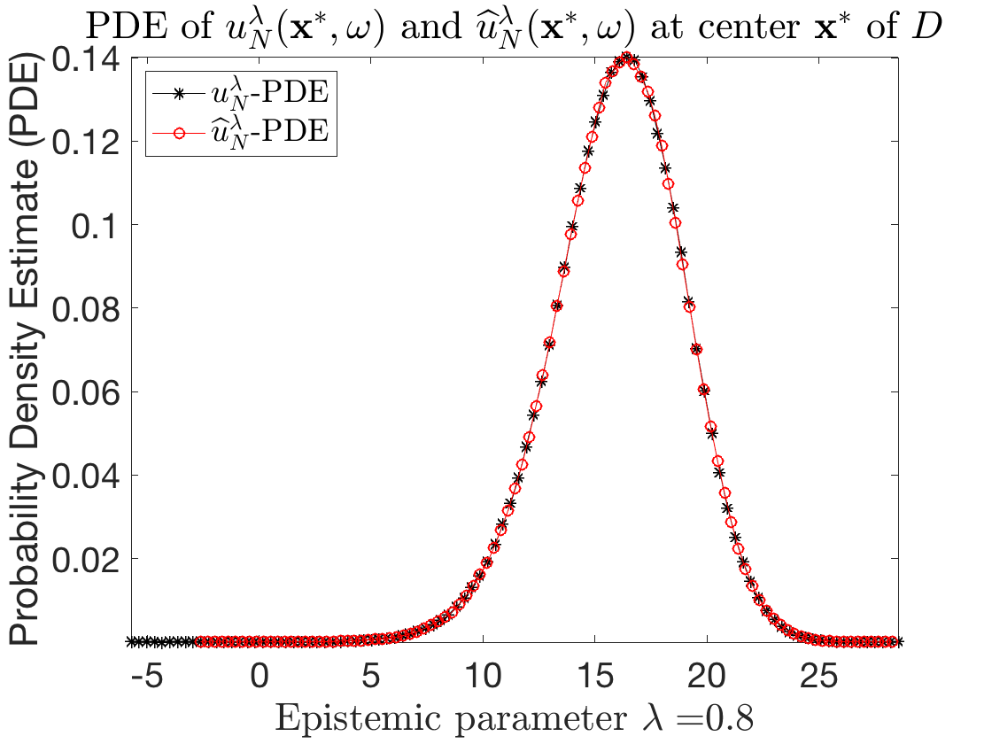
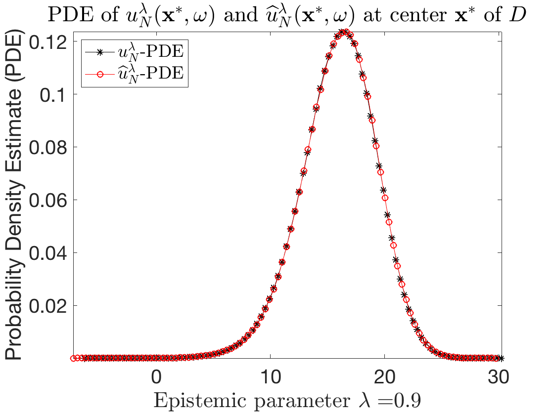
(g) $\tau=0.7$	(h) $\tau=0.8$	(i) $\tau=0.9$

Figure 8: Ten-dimensional stochastic diffusion model: Comparisons of probability density estimates (PDE) of the gPC solution $u_{N}^{\tau}(\boldsymbol{x}^{*},\omega)$ and corresponding post-processed surrogate $\widehat{u}_{N}^{\tau}(\boldsymbol{x}^{*},\omega)$ at the center $\boldsymbol{x}^{*}$ of $D$, and for various epistemic parameter values.

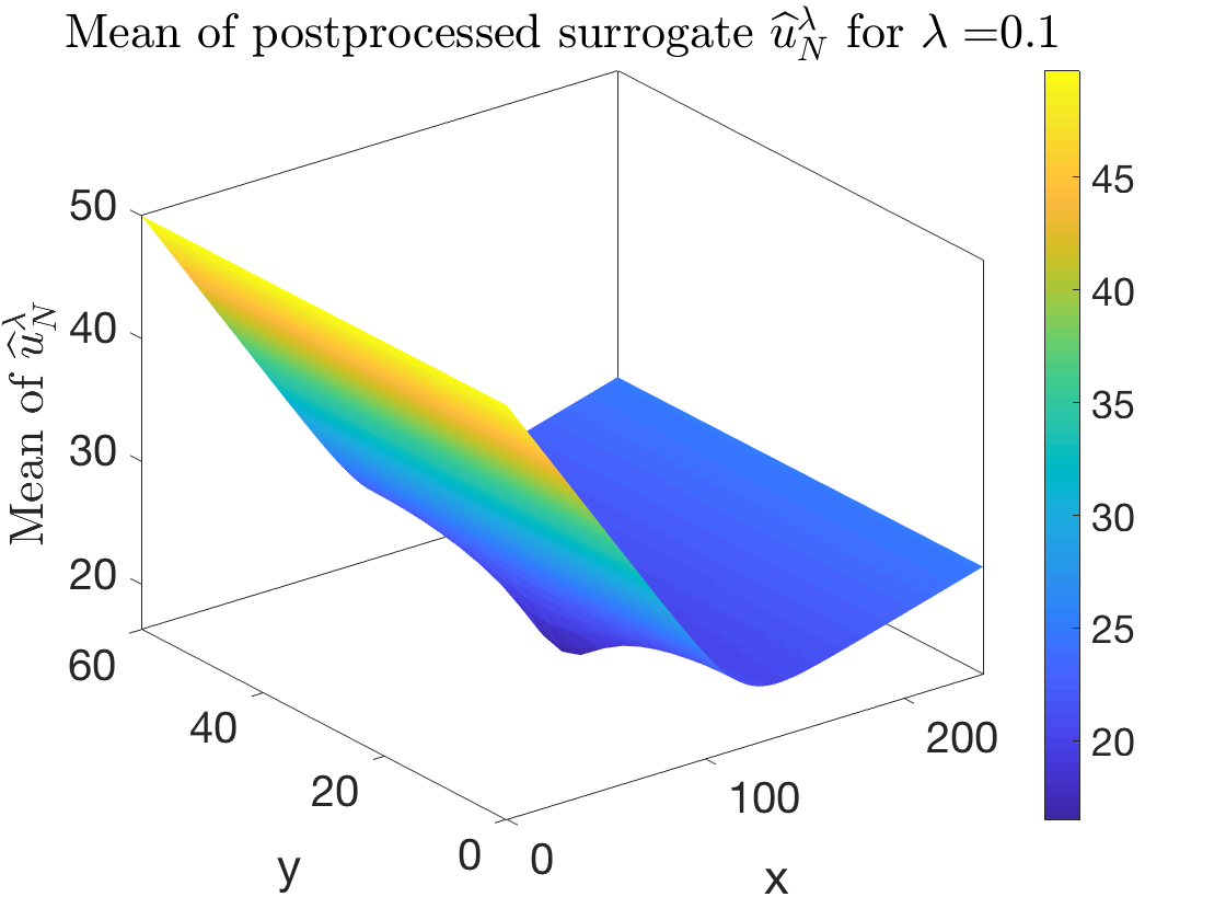
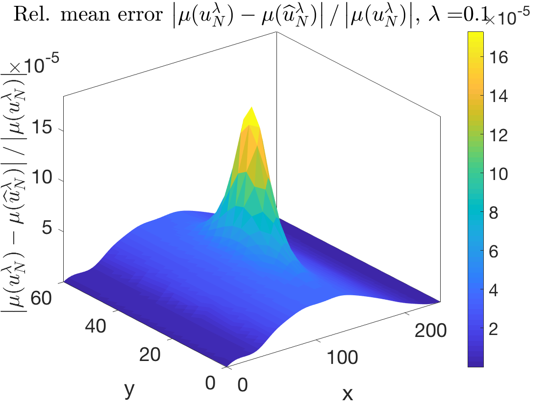
(a) $\tau=0.1$, gPC mean solution $u_{N}^{\tau}$	(b) $\tau=0.1$, post-processed surrogate mean solution $\widehat{u}_{N}^{\tau}$	(c) $\tau=0.1$, relative error of mean solutions

Figure 9: Ten-dimensional stochastic diffusion model: Comparisons of the mean gPC solution $u_{N}^{\tau}$ and the mean of corresponding post-processed surrogate $\widehat{u}_{N}^{\tau}$ for $\tau=0.1$.

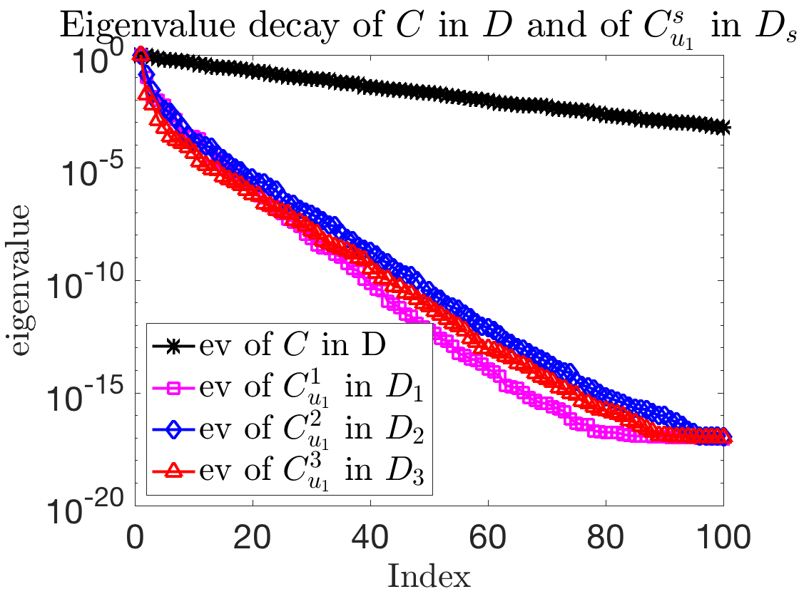
Figure 10: Decay of the eigenvalues of the given covariance matrix $C(\boldsymbol{x},\boldsymbol{y})$ at grid points in $D\times D$ and the coarse solution $u_{1}$ based covariance matrix $C^{s}_{u_{1}}(\boldsymbol{x},\boldsymbol{y})$ at grid points in the sub-domains $D_{s}\times D_{s}$, for $s=1,2,3$, where $D=\cup_{s=1}^{8}D_{s}$.

$\tau$	max. rel. mean error	max. rel. variance error
0.9	8.8316e-05	1.2265e-03
0.8	1.5066e-04	2.2016e-03
0.7	1.9168e-04	2.9742e-03
0.6	2.2377e-04	3.8097e-03
0.5	2.4742e-04	4.5387e-03
0.4	2.6353e-04	5.1387e-03
0.3	2.7460e-04	5.6057e-03
0.2	2.8140e-04	5.9388e-03
0.1	2.8503e-04	6.1383e-03

Table 8: Hundred-dimensional stochastic diffusion model: Maximum norm relative error of the approximate mean and variance computed using the DD-gPC approach and the post-processed surrogate method.

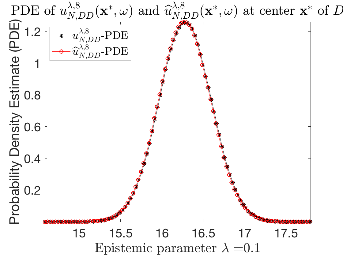
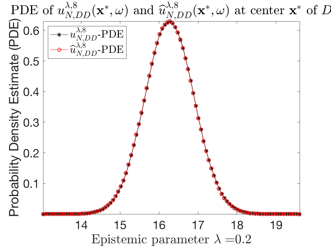
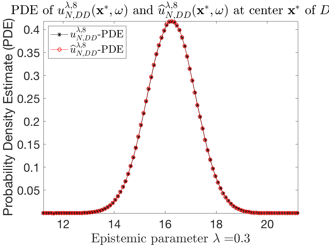
(a) $\tau=0.1$	(b) $\tau=0.2$	(c) $\tau=0.3$
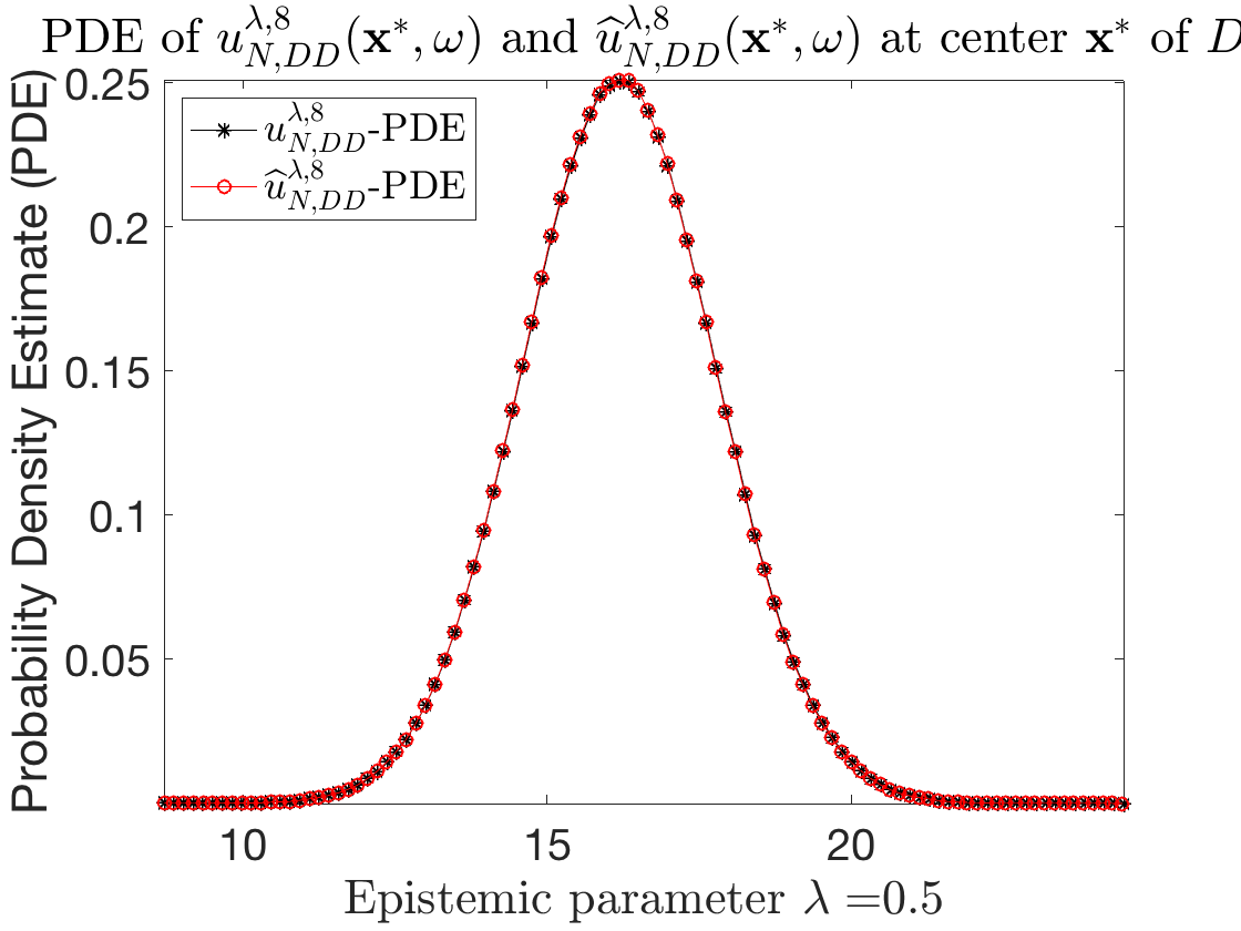
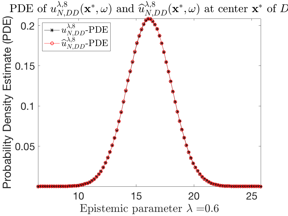
(d) $\tau=0.4$	(e) $\tau=0.5$	(f) $\tau=0.6$
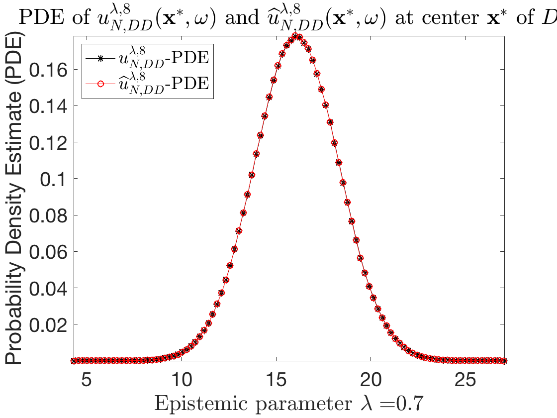
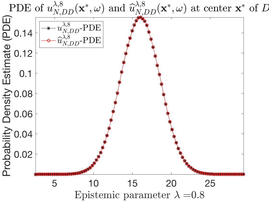
(g) $\tau=0.7$	(h) $\tau=0.8$	(i) $\tau=0.9$

Figure 11: Hundred-dimensional stochastic diffusion model: Comparisons of probability density estimates (PDE) of the gPC-DD solution $u_{N,DD}^{\tau,8}(\boldsymbol{x}^{*},\omega)$ and corresponding post-processed surrogate $\widehat{u}_{N,DD}^{\tau,8}(\boldsymbol{x}^{*},\omega)$ at the center $\boldsymbol{x}^{*}$ of $D$, and for various epistemic parameter values.

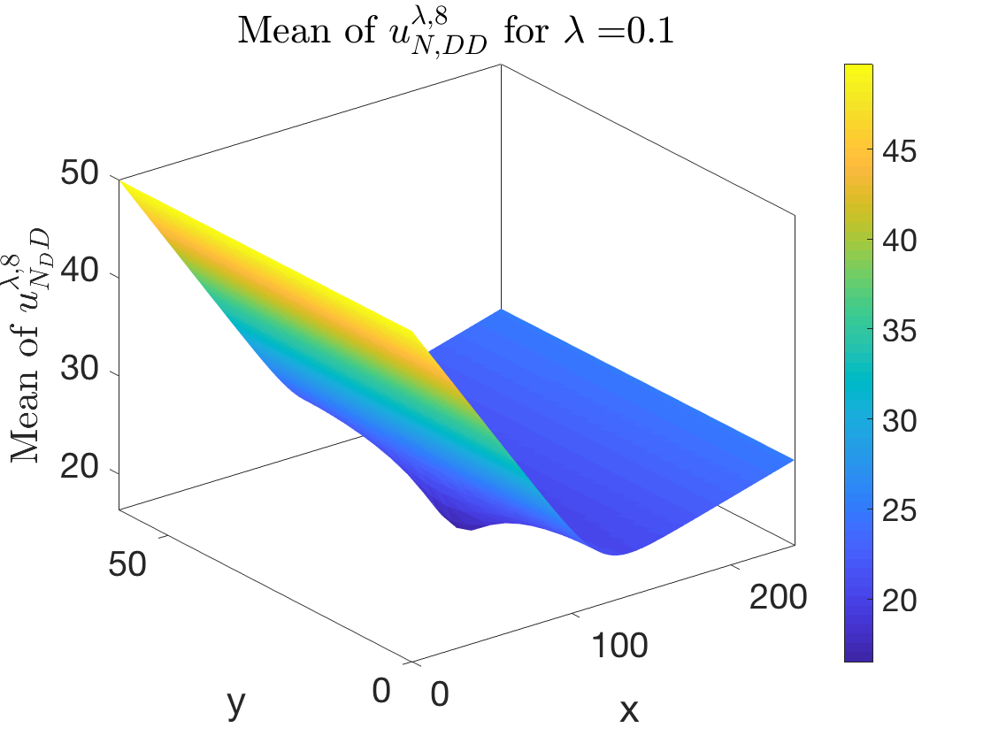
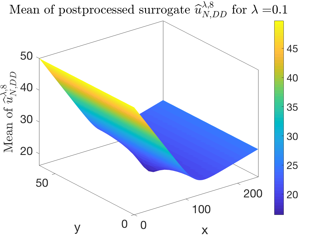
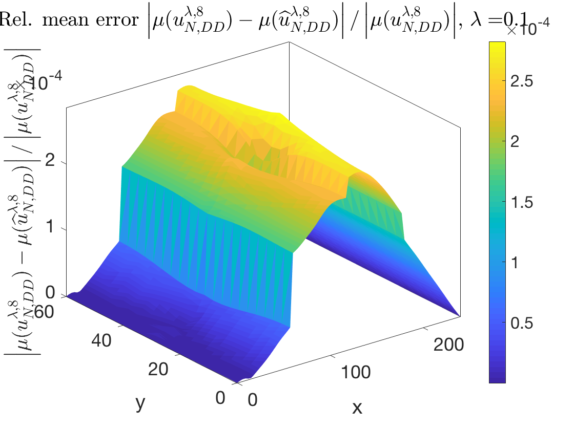
(a) $\tau=0.1$, gPC-DD mean solution $u_{N,DD}^{\tau,8}$	(b) $\tau=0.1$, post-processed surrogate mean solution $\widehat{u}_{N,DD}^{\tau,8}$	(c) $\tau=0.1$, relative error of mean solutions

Figure 12: Hundred-dimensional stochastic diffusion model: Comparisons of the mean gPC-DD solution $u_{N,DD}^{\tau,8}$ and the mean of corresponding post-processed surrogate $\widehat{u}_{N,DD}^{\tau,8}$ for $\tau=0.1$.

References

- [1] J.-C. Nédélec, Acoustic and Electromagnetic Equations, Springer, 2001.
- [2] D. Colton, R. Kress, Inverse Acoustic and Electromagnetic Scattering Theory, Springer, 2012.
- [3] M. Ganesh, S. Hawkins, D. Volkov, An efficient algorithm for a class of stochastic forward and inverse Maxwell models in , J. Comput. Phys. 398 (2019) 108881.
- [4] V. Dominguez, M. Ganesh, F. Sayas, An overlapping decomposition framework for wave propagation in heterogeneous and unbounded media: Formulation, analysis, algorithm, and simulation, J. Comput. Phys. 403 (2020) 109052.
-
[5]
M. Ganesh, C. Morgenstern, A
coercive heterogeneous media Helmholtz model: formulation,
wavenumber-explicit analysis, and preconditioned high-order FEM, Numerical
Algorithms (2020) to appear (47 pages).
URL https://doi.org/10.1007/s11075-019-00732-8 - [6] J. Dick, F. Y. Kuo, I. H. Sloan, High-dimensional integration - the quasi-Monte Carlo way, Acta Numerica, 22 (2013) 133–288.
- [7] O. P. L. Maitre, O. M. Kino, Spectral Methods for Uncertainty Quantification, Springer, 2010.
- [8] H. Lei, J. Lia, P. Gao, P. Stinis, N. A. Baker, A data-driven framework for sparsity-enhanced surrogates with arbitrary mutually dependent randomness, Comput. Methods Appl. Mech. Engrg. 350 (2019) 199–2827.
- [9] R. Tipireddy, R. Ghanem, Basis adaptation in homogeneous chaos spaces, Journal of Computational Physics 259 (2014) 304–317.
- [10] M. Ganesh, S. C. Hawkins, A high performance computing and sensitivity analysis algorithm for stochastic many-particle wave scattering, SIAM J. Sci. Comput. 37 (2015) A1475–A1503.
- [11] M. Ganesh, S. C. Hawkins, An offline/online algorithm for a class of stochastic multiple obstacle configurations in half-plane, J. Comp. Appl. Math. 307 (2016) 52–64.
- [12] R. Tipireddy, P. Stinis, A. Tartakovsky, Basis adaptation and domain decomposition for steady-state partial differential equations with random coefficients, Journal of Computational Physics 351 (2017) 203–215.
- [13] R. Tipireddy, P. Stinis, A. M. Tartakovsky, Stochastic basis adaption and spatial domain decomposition for partial differential equations with random coefficients, ASA/SIAM J. Uncertainty Quantification 6 (2018) 273–301.
- [14] S. C. Hawkins, Algorithm xxx: MieSolver—an object-oriented Mie Series software for wave scattering by cylinders, ACM Trans. Math. Softw.(submitted).
- [15] Rayleigh, On the electromagnetic theory of light, Philos. Mag. S. 5 12 (73).
- [16] G. Mie, Beiträge zur optik trüber medien speziell kolloidaler matallösungen, Ann Phys. 25 (1908) 377–445.
- [17] H. C. van de Hulst, Light Scattering by Small Particles, Dover Publications Inc., 1981.
- [18] C. F. Bohren, D. R. Huffman, Absorption and Scattering of Light by Small Particles, Wiley, 1983.
- [19] T. Rother, M. Kahnert, Electromagnetic wave scattering on nonspherical particles: basic methodology and simulations, 2nd Edition, Springer, 2013.