Asynchronous $\epsilon$-Greedy Bayesian Optimisation

Abstract

Batch Bayesian optimisation (BO) is a successful technique for the optimisation of expensive black-box functions. Asynchronous BO can reduce wallclock time by starting a new evaluation as soon as another finishes, thus maximising resource utilisation. To maximise resource allocation, we develop a novel asynchronous BO method, AEGiS (Asynchronous $\epsilon$-Greedy Global Search) that combines greedy search, exploiting the surrogate’s mean prediction, with Thompson sampling and random selection from the approximate Pareto set describing the trade-off between exploitation (surrogate mean prediction) and exploration (surrogate posterior variance). We demonstrate empirically the efficacy of AEGiS on synthetic benchmark problems, meta-surrogate hyperparameter tuning problems and real-world problems, showing that AEGiS generally outperforms existing methods for asynchronous BO. When a single worker is available performance is no worse than BO using expected improvement.

1 Introduction

Bayesian Optimisation (BO) is a popular sequential approach for optimising time-consuming or costly black-box functions that have no closed-form expression or derivative information [Brochu et al., 2010, Snoek et al., 2012]. BO comprises two main steps which are repeated until convergence or the budget is exhausted. Firstly, a surrogate model is constructed using previous evaluations; this is typically a Gaussian process (GP), due to its strength in uncertainty quantification and function approximation [Rasmussen and Williams, 2006, Shahriari et al., 2016]. Secondly, an acquisition function is optimised to select the next location to expensively evaluate. Such functions attempt to balance the exploitation of locations with a good predicted value with the exploration of locations with high uncertainty.

In real-world problems it is often possible to use hardware capabilities to run multiple evaluations in parallel. For example, the number of hyperparameter configurations that can be evaluated in parallel when training neural networks [Chen et al., 2018] is only limited by the computational resources available. The desire to speed up optimisation wallclock time through parallel evaluation led to the development of parallel BO in which $q$ locations are jointly selected to be evaluated synchronously. It has been successfully applied in many areas such as drug discovery [Hernández-Lobato et al., 2017], heat treatment, [Gupta et al., 2018], and hyperparameter configuration [Kandasamy et al., 2018].

When the runtime for evaluations varies, such as when optimising the number of units in the layers of a neural network, or indeed the number of layers themselves, synchronous parallel approaches will result in resource underutilisation because all evaluations must finish before the next $q$ locations can be suggested. To counteract this, asynchronous BO approaches have been proposed that allow for the evaluation of functions asynchronously; i.e., as soon as an evaluation has completed, another can be submitted. In order to take into account the uncertainty in the surrogate model at and around locations which are still being evaluated, a number of methods have been proposed to penalise either the surrogate model itself or the acquisition function in order to limit the selection of locations near places that are currently under evaluation [Ginsbourger et al., 2008, González et al., 2016, Alvi et al., 2019].

Kandasamy et al. [2018] presented an alternative approach based on Thompson sampling (TS) that draws surrogate function realisations from the GP posterior and optimises these to suggest new locations to evaluate without the need to penalise the model or acquisition function. However, TS relies on there being enough stochasticity to create sufficiently diverse function draws with meaningfully different optima. Therefore, TS tends to be insufficiently exploratory in low dimensions (as draws are very similar to the mean prediction) and over-exploratory in high dimensions where the posterior uncertainty is large across much of the domain.

$\epsilon$-greedy methods have been shown to be remarkably successful in sequential and synchronous parallel optimisation [De Ath et al., 2020, De Ath et al., 2021]. Most of the time these exploit the mean prediction of the surrogate model by expensively evaluating the location with the best posterior mean, ignoring the uncertainty in the surrogate’s prediction, but making deliberately exploratory samples with probability $\epsilon$. In this work we combine a greedy exploitation of the mean prediction with Thompson sampling and random selection from the approximate Pareto set that maximally trades off exploration and exploitation. Specifically, we introduce an $\epsilon$-greedy scheme that, with probability $\epsilon_{T}$ performs Thompson sampling or with probability $\epsilon_{P}$ random selection from the approximate Pareto set, and exploits the surrogate model’s posterior mean prediction the rest of the time, i.e. with probability $1-(\epsilon_{T}+\epsilon_{P})$. For convenience we write $\epsilon=\epsilon_{T}+\epsilon_{P}$. One of the reasons for the success of $\epsilon$-greedy methods is that model inaccuracy introduces some accidental exploration even when exploiting the mean prediction. This effect becomes dominant as the dimension increases, and we therefore investigate how $\epsilon$ can be reduced with increasing dimension.

• We present AEGiS (Asynchronous $\epsilon$-Greedy Global Search), a novel asynchronous BO algorithm that combines greedy exploitation of the posterior mean prediction with Thompson sampling and random selection from the approximate Pareto set between exploration and exploitation.

• We present results on fifteen well-known benchmark functions, three meta-surrogate hyperparameter tuning problems and two robot pushing problems. Empirically, we demonstrate that AEGiS outperforms existing methods for asynchronous BO on synthetic and hyperparameter optimisation problems.

• We investigate how the degree of deliberate exploration $\epsilon$ should be controlled with increasing dimension, $d$, showing empirically that $\epsilon=\min(2/\sqrt{d},1)$ yields superior performance to increased or decreased rates of exploration with respect to problem dimensionality.

• We present an ablation study that verifies the importance of all three components, namely the Pareto set selection, Thompson sampling, and exploitation, showing that AEGiS achieves performance that is greater than the sum of its individual components.

• We show empirically that selection from the exploration-exploitation Pareto set is superior to selection from the entire problem domain.

We begin in Section 2 by reviewing sequential, synchronous and asynchronous BO, and Thompson sampling, before introducing AEGiS in Section 3. Section 4 details extensive empirical evaluation of AEGiS against other popular methods on well-known test problems, and also includes an ablation study. We finish with concluding remarks in Section 5.

2 Bayesian Optimisation

Our goal is to minimise a black-box function $f:\mathcal{X}\mapsto\mathbb{R}$, defined on a compact domain $\mathcal{X}\subset\mathbb{R}^{d}$. The function itself is unknown, but we have access to the result of its evaluation $f(\mathbf{x})$ at any location $\mathbf{x}\in\mathcal{X}$. We are particularly interested in cases where the evaluations are expensive, either in terms of time or money or both. We therefore seek to minimise $f$ in either as few evaluations as possible to incur as little cost as possible or for a fixed budget.

2.1 Sequential Bayesian Optimisation

Bayesian Optimisation (BO) is a global search strategy that sequentially samples the problem domain $\mathcal{X}$ at locations that are likely to contain the global optimum, taking into account both the predictions of a probabilistic surrogate model and its corresponding uncertainty [Jones et al., 1998]. It starts by generating $M$ initial sample locations $\{\mathbf{x}_{i}\}_{i=1}^{M}$ with a space filling algorithm, such as Latin hypercube sampling [McKay et al., 1979], and expensively evaluates them with the function $f_{i}=f(\mathbf{x}_{i})$. This set of observations $\mathcal{D}_{M}=\{(\mathbf{x}_{n},f_{n}\triangleq f(\mathbf{x}_{n}))\}_{n=1}^{M}$ is used for initial training of the surrogate model. Following training, and at each iteration of BO, the next location to be expensively evaluated is chosen as the location that maximises an acquisition function $\alpha(\mathbf{x})$. Thus $f(\cdot)$ is next evaluated at $\mathbf{x}^{\prime}=\operatorname*{\arg\!\max}_{\mathbf{x}\in\mathcal{X}}\alpha(\mathbf{x})$. The dataset is augmented with $\mathbf{x}^{\prime}$ and $f(\mathbf{x}^{\prime})$ and the process is repeated until the budget is exhausted. The value of the global minimum is then estimated to be the best function evaluation seen during optimisation, i.e. $f^{\star}=\min_{i}\{f_{i}\}$.

Gaussian Processes

Gaussian processes (GPs) are commonly used as the surrogate model for $f$. A GP defines a prior distribution over functions, such that any finite number of function values have a joint Gaussian distribution [Rasmussen and Williams, 2006] with mean $m(\mathbf{x})$ and a covariance $\kappa(\mathbf{x},\mathbf{x}^{\prime}\,|\,\boldsymbol{\theta})$ with hyperparameters $\boldsymbol{\theta}$. Henceforth, w.l.o.g. we use a zero-mean prior $m(\mathbf{x})=0\,\forall\,\mathbf{x}\in\mathcal{X}$. Conditioning the prior distribution on data consisting of $f$ evaluated at $t$ sampled locations $\mathcal{D}_{t}$, the posterior distribution of $f$ is also a GP with posterior mean and variance

$$\mu(\mathbf{x}\,|\,\mathcal{D},\boldsymbol{\theta}) =m(\mathbf{x})+\boldsymbol{\kappa}(\mathbf{x},X)K^{-1}\mathbf{f}$$ (1)

$$\sigma^{2}(\mathbf{x}\,|\,\mathcal{D},\boldsymbol{\theta}) =\kappa(\mathbf{x},\mathbf{x})-\boldsymbol{\kappa}(\mathbf{x},X)^{\top}K^{-1}\boldsymbol{\kappa}(X,\mathbf{x}).$$ (2)

Here, $X\in\mathbb{R}^{t\times d}$ and $\mathbf{f}=(f_{1},f_{2},\dots,f_{t})^{\top}$ are the matrix of design locations and corresponding vector of function evaluations respectively. The kernel matrix $K\in\mathbb{R}^{t\times t}$ is $K_{ij}=\kappa(\mathbf{x}_{i},\mathbf{x}_{j}\,|\,\boldsymbol{\theta})$ and $\boldsymbol{\kappa}(\mathbf{x},X)\in\mathbb{R}^{t}$ is given by $[\boldsymbol{\kappa}(\mathbf{x},X)]_{i}=\kappa(\mathbf{x},\mathbf{x}_{i}\,|\,\boldsymbol{\theta})$. Kernel hyperparameters $\boldsymbol{\theta}$ are learnt by maximising the log marginal likelihood [Rasmussen and Williams, 2006].

Acquisition Functions

The choice of where to evaluate next in BO is determined by an acquisition function ${\alpha:\mathbb{R}^{d}\mapsto\mathbb{R}}$. Perhaps the most commonly used acquisition function is Expected Improvement (EI) [Jones et al., 1998], which is defined as the expected positive improvement over the best-seen function value $f^{\star}$ thus far:

$$\alpha_{\text{EI}}(\mathbf{x})=\mathbb{E}_{p(f(\mathbf{x})\,|\,\mathcal{D})}\left[\max\left(f^{\star}-f(\mathbf{x}),\,0\right)\right].$$ (3)

However, many other acquisition functions have also been proposed, including probability of improvement [Kushner, 1964], optimistic strategies such as UCB [Srinivas et al., 2010], $\epsilon$-greedy strategies [Bull, 2011, De Ath et al., 2021], and information-theoretic approaches [Scott et al., 2011, Hennig and Schuler, 2012, Henrández-Lobato et al., 2014, Wang and Jegelka, 2017, Ru et al., 2018].

2.2 Parallel Bayesian Optimisation

In parallel BO, the algorithm has access to $q$ workers that can evaluate $f$ in parallel and the focus is on minimising the optimisation time, acknowledging that the total computational cost will be greater than for strictly sequential evaluations. The goal is to select a batch of $q$ promising locations to be expensively evaluated in parallel. In the synchronous setting, the BO algorithm sends out a batch of $q$ locations to be evaluated in parallel, and waits for all $q$ evaluations to be completed before submitting the next batch. However, in the asynchronous setting, as soon as a worker has finished evaluating $f$ a new location is submitted to it for evaluation. Therefore, if $f$ takes a variable time to evaluate, the asynchronous version of BO will result in more evaluations of $f$ for the same wallclock time.

One of the earliest synchronous approaches was the qEI method of Ginsbourger et al. [2008], a generalisation of the sequential EI acquisition function (3) that jointly proposes a batch of $q$ locations to evaluate. Similarly, the parallel predictive entropy search [Shah and Ghahramani, 2015] and the parallel knowledge gradient [Wu and Frazier, 2016] also jointly propose $q$ locations and are based on their sequential counterparts. However, these methods require the optimisation of a $d\times q$ problem that becomes prohibitively expensive to solve as $q$ increases [Daxberger and Low, 2017].

Consequently, the prevailing strategy has become to sequentially select the $q$ batch locations. Penalisation-based methods penalise the regions of either the surrogate model [Azimi et al., 2010, Desautels et al., 2014] or the acquisition function that correspond to locations that are currently under evaluation. The Kriging Believer method of Ginsbourger et al. [2010], for example, hallucinates the results of pending evaluations by using the surrogate model’s mean prediction as its observed value. The local penalisation methods of González et al. [2016] and Alvi et al. [2019] directly penalise an acquisition function. De Ath et al. [2020] show that an $\epsilon$-greedy method that usually exploits the most promising region, with occasional exploratory moves, is effective.

Asynchronous BO has received less attention. Janusevskis et al. [2012] proposed an asynchronous version of the qEI method that uses the qEI criterion assuming that the $p$ locations currently under evaluation are fixed, and optimises the position of the remaining $q-p$ locations. Kandasamy et al. [2018] suggest using Thompson sampling to select locations to evaluate. Thompson sampling (TS) [Thompson, 1933] is a randomised strategy for sequential decision-making under uncertainty [Kandasamy et al., 2018]. At each iteration, TS selects the next location to evaluate $\mathbf{x}^{\prime}$ according to the posterior probability that it is the optimum. If $p_{*}(\mathbf{x}\,|\,\mathcal{D})$ denotes the probability that $\mathbf{x}$ minimises the surrogate model posterior, then

$$p_{*}(\mathbf{x}\,|\,\mathcal{D}) =\int p_{*}(\mathbf{x}\,|\,g)\,p(g\,|\,\mathcal{D})\,dg$$ (4)

$$=\int\delta(\mathbf{x}-\operatorname*{\arg\!\min}_{\mathbf{x}\in\mathcal{X}}g(\mathbf{x}))\,p(g\,|\,\mathcal{D})\,dg,$$ (5)

where $\delta$ is the Dirac delta distribution. Thus, all the probability mass of $p_{*}(\mathbf{x}\,|\,\mathcal{D})$ is at the minimiser of $g$. In the context of BO, this corresponds to sampling a function $g(\cdot)$ from the surrogate model’s posterior $p(\cdot\,|\,\mathbf{x},\mathcal{D})$ and selecting $\mathbf{x}^{\prime}=\operatorname*{\arg\!\min}_{\mathbf{x}\in\mathcal{X}}g(\mathbf{x})$ as the next location to evaluate. This can then be trivially applied in the sequential, synchronous and asynchronous settings by sampling and minimising as many function realisations as required. Thus, the BO loop using TS involves building a surrogate model with previously evaluated locations (ignoring those that may be currently under evaluation), drawing as many function realisations as there are free workers, finding the minimiser of each realisation and evaluating $f$ at those locations.

Kandasamy et al. [2018] analyse Thompson sampling in terms of maximum information gain. They show that both synchronous and asynchronous TS algorithms making $n$ function evaluations are almost as good as if the $n$ evaluations were made sequentially. Furthermore, they extend the notion of simple regret to incorporate the (random) number of evaluations made in a given time. Under this metric they show that asynchronous TS outperforms synchronous and sequential algorithms using a variety of evaluation-time models.

Traditionally, $g$ has been approximately optimised by picking the minimum of a randomly sampled set of discrete points [Kandasamy et al., 2018]. Recently, Wilson et al. [2020] have identified an elegant decoupled sampling method, which we use here, that decomposes the GP posterior into a sum of a weight-space prior term that is approximated by random Fourier features, and a pathwise update in function space. Unlike other fast approximations, such as [Rahimi and Recht, 2008], this method does not suffer from variance starvation [Calandriello et al., 2019]. It scales linearly with the number of locations queried during optimisation of $g$, and is pathwise differentiable, meaning that gradient-based optimisation can be employed.

Recently, De Palma et al. [2019] proposed to draw realisations of acquisition functions instead, by drawing a new set of surrogate model hyperparameters from their posterior distribution for each acquisition function. An advantage of these TS-based methods is that each draw from either the model or hyperparameter posterior defines a new distinct acquisition function. A drawback is that they rely on the uncertainty in the surrogate model to give sufficient diversity in position to the locations selected, unlike acquisition functions which implicitly or explicitly balance exploration and exploitation.

3 AEGiS

It is well recognised that the fundamental problem in global optimisation is to balance exploitation of promising locations found thus far with exploration of new areas which have not been explored. While extremely appealing in its simplicity, Thompson sampling (TS) tends to over-exploit in low dimensions (because after a number of evaluations the posterior variance is reduced and most sampled realisations are similar to the posterior mean), but under-exploit in high dimensions (because there are insufficient samples to drive the posterior variance away from the prior, resulting in effectively random search). The efficacy of $\epsilon$-greedy methods in sequential and synchronous BO over a range of dimensions [De Ath et al., 2020, De Ath et al., 2021] motivates an $\epsilon$-greedy strategy to switch between greedy exploitation of the surrogate model, exploration, and TS. Specifically, at each step we optimise a TS function draw with probability $\epsilon_{T}$ or perform exploration each with probability $\epsilon_{P}$, and exploit the surrogate model’s posterior mean prediction $\mu(\mathbf{x})$ of the rest of the time, i.e. with probability $1-(\epsilon_{T}+\epsilon_{P})$.

Algorithm 1 AEGiS

1:Inputs: $\mathcal{D}_{t}$: Training data; $T$: Evaluation budget

2:$M=|\mathcal{D}_{t}|$

3:for $t=M+1,\dots,T$ do

4:    Condition model posterior on $\mathcal{D}_{t}$; see (1) and (2)

5:    $r\sim\mathcal{U}(0,1)$

6:    if  $r<1-(\epsilon_{T}+\epsilon_{P})$  then $\triangleright$ Exploit surrogate model

7:         $\mathbf{x}^{\prime}\leftarrow\underset{\mathbf{x}\in\mathcal{X}}{\operatorname*{\arg\!\min}}\,\mu(\mathbf{x})$

8:    else if $r<1-\epsilon_{P}$ then $\triangleright$ Thompson sample

9:         $g\sim p(f\,|\,\mathcal{D})$

10:         $\mathbf{x}^{\prime}\leftarrow\underset{\mathbf{x}\in\mathcal{X}}{\operatorname*{\arg\!\min}}\,g(\mathbf{x})$

11:    else$\triangleright$ Approximate Pareto set selection

12:         $\tilde{\mathcal{P}}\leftarrow\mathtt{MOOptimise}_{\mathbf{x}\in\mathcal{X}}(\mu(\mathbf{x}),\sigma^{2}(\mathbf{x}))$

13:         $\mathbf{x}^{\prime}\leftarrow\mathtt{randomChoice}(\tilde{\mathcal{P}})$     

14:    Submit new job to evaluate $\mathbf{x}^{\prime}$

15:    while all workers in use do

16:         Wait for a worker to finish     

17:    $\mathcal{D}_{t}\leftarrow\mathcal{D}_{t-1}\cup\{(\mathbf{x}^{\prime},f(\mathbf{x}^{\prime}))\}$ $\triangleright$ Augment data

The AEGiS method is outlined in Algorithm 1. With probability $1-(\epsilon_{T}+\epsilon_{P})$, the mean prediction from the surrogate model is minimised to find the next location $\mathbf{x}^{\prime}$ to evaluate (line 7). Alternatively, with probability $\epsilon_{T}$, a TS step taken: the next location is determined by sampling a realisation $g(\cdot)$ from the surrogate posterior and finding its minimiser (lines 9 and 10). Otherwise (lines 12 and 13), with probability $\epsilon_{P}$, the location to evaluate is chosen from the approximate Pareto set of all locations which maximally trade off between exploitation (minimising $\mu(\mathbf{x})$) and exploration (maximising $\sigma^{2}(\mathbf{x})$). A full discussion is given by De Ath et al. [2021]. Briefly, a location $\mathbf{x}_{1}$ dominates $\mathbf{x}_{2}$ (written $\mathbf{x}_{1}\succ\mathbf{x}_{2}$) iff $\mu(\mathbf{x}_{1})\leq\mu(\mathbf{x}_{2})$ and $\sigma(\mathbf{x}_{1})\geq\sigma(\mathbf{x}_{2})$, and at least one of the inequalities is strict. If both $\mathbf{x}_{1}\nsucc\mathbf{x}_{2}$ and $\mathbf{x}_{2}\nsucc\mathbf{x}_{1}$ then $\mathbf{x}_{1}$ and $\mathbf{x}_{2}$ are said to be mutually non-dominating. The maximal set of mutually non-dominating solutions is known as the Pareto set $\mathcal{P}=\{\mathbf{x}\in\mathcal{X}\,|\,\mathbf{x}^{\prime}\not\succ\mathbf{x}\,\forall\mathbf{x}^{\prime}\in\mathcal{X}\}$ and comprises the optimal trade-off between exploratory and exploitative locations. Since it is infeasible to enumerate $\mathcal{X}$, we sample a location from the approximate Pareto set $\tilde{\mathcal{P}}\approx\mathcal{P}$ which is found using a standard multi-objective optimiser (lines 12 and 13).

Selecting a random location from $\tilde{\mathcal{P}}$ ensures that no other location could have been selected that has either more uncertainty given the same predicted value or a lower predicted value given the same amount of uncertainty. Therefore, when considering the two objectives of both reducing the overall model uncertainty and finding the location with the minimum value, these locations are optimal with respect to a specific exploitation-exploration trade-off. Indeed, the maximisers of both EI and UCB are members of $\mathcal{P}$ [De Ath et al., 2021].

Rather than selecting from $\tilde{\mathcal{P}}$, a more exploratory procedure is to select from the entire feasible space $\mathcal{X}$. That is, lines 12 and 13 are replaced with $\mathbf{x}^{\prime}\leftarrow\mathtt{randomChoice}(\mathcal{X})$. We denote this variant by AEGiS-RS. However, as shown below, it is less effective than selection from $\tilde{\mathcal{P}}$.

At the beginning of an optimisation run, the initial $q$ locations to be evaluated are chosen by first selecting the most exploitative location (line 7). The remaining $q-1$ locations are each chosen by performing either Thompson sampling or selection from the approximate Pareto set $\tilde{\mathcal{P}}$ with probabilities $\epsilon_{T}/(\epsilon_{T}+\epsilon_{P})$ and $\epsilon_{P}/(\epsilon_{T}+\epsilon_{P})$ respectively. This ensures that the most exploitative location is only chosen once during initialisation. The remaining evaluated locations in an optimisation run are chosen according to Algorithm 1.

As discussed above, inaccuracies in the surrogate model provide an element of exploration even when disregarding the uncertainty in the posterior $p(f\,|\,\mathcal{D}_{t})$. On the other hand, TS tends to be over-exploitative in low dimensions ($d\lesssim 4$) and too exploratory in high dimensions. The performance of sequential $\epsilon$-greedy algorithms is relatively insensitive to the precise choice of $\epsilon$ [De Ath et al., 2021]. As we show in section 4.4, the performance of AEGiS is relatively insensitive to the ratio of $\epsilon_{T}:\epsilon_{P}$. For simplicity, we therefore initially set $\epsilon_{T}=\epsilon_{P}=\epsilon/2$ and $\epsilon=\min(2/\sqrt{d},1)$. This allows for more exploitation to occur as the dimensionality of the problem increases. As shown empirically in section 4.4, this rate of decay in the amount of exploration carried out with respect to the problem dimensionality is more effective than faster or slower rates.

The dominant contributor to computational cost of finding the approximate Pareto set, carried out by NSGA-II [Deb et al., 2002], is the non-dominated sort of the population of solutions and their offspring. With two objectives, as is the case in AEGiS, this has complexity $\mathcal{O}(GN\log N)$ [Jensen, 2003], where $N$ is the total population size and $G$ is the number of generations for which the evolutionary algorithm runs. Empirically we find that this cost is similar to that of TS, whose computational cost is dominated by the gradient descent method used to optimise the sample path $g$; e.g. $\mathcal{O}(Ld^{2})$ for BFGS [Byrd et al., 1995], where $L$ is the maximum number of steps taken in the search. However, we note that both of these costs are negligible compared to fitting the GP.

4 Experimental Evaluation

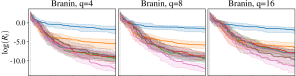
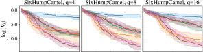
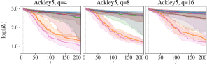
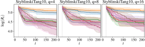
Figure 1: Illustrative convergence plots for four benchmark problems with $q\in\{4,8,16\}$ asynchronous workers. Each plot shows the median log simple regret, with shading representing the interquartile range over $51$ runs.

We compare AEGiS with four well-known asynchronous BO algorithms: two acquisition function-based penalisation methods, Local Penalisation (LP) [González et al., 2016] and the more recent PLAyBOOK [Alvi et al., 2019], as well as the Kriging Believer (KB) [Ginsbourger et al., 2010], all of which are based on the expected improvement acquisition function (3). We also include the standard Thompson sampling (TS) approach of Kandasamy et al. [2018] and a purely random approach using Latin hypercube sampling (Random). The optimisation pipeline was constructed using GPyTorch [Gardner et al., 2018] and BoTorch [Balandat et al., 2020], and we have made this available online.

A zero-mean Gaussian process surrogate model with an isotropic Matérn $5/2$ kernel, as recommended by Snoek et al. [2012] for modelling realistic functions, was used in all the experiments. Input variables were rescaled to reside in $[0,1]^{d}$ and observations were rescaled to have zero-mean and unit variance. The models were initially trained on $M=2d$ observations generated by maximin Latin hypercube sampling and then optimised for a further $200-2d$ function evaluations. Each optimisation run was repeated $51$ times from a different set of Latin hypercube samples. Sets of initial locations were common across all methods to enable statistical comparison. At each iteration, before new locations were selected, the hyperparameters of the GP were optimised by maximising the log likelihood using a multi-restart strategy [Shahriari et al., 2016] with L-BFGS-B [Byrd et al., 1995] and $10$ restarts (Algorithm 1, line 4).

All experiments were repeated for $q\in\{4,8,16\}$ asynchronous workers. We followed the procedure of Kandasamy et al. [2018] to sample an evaluation time for each task, thereby simulating the asynchronous setting. A half-normal distribution was used for this with a scale parameter of $\sqrt{\pi/2}$, giving a mean runtime of 1 [Alvi et al., 2019].

The KB, LP and PLAyBOOK methods all used the EI acquisition function, which was selected because of its popularity. The expected improvement, the sampled function from the GP posterior in both TS and AEGiS, and the posterior mean in AEGiS were all optimised using the typical strategy [Balandat et al., 2020] of uniformly sampling $1000d$ locations in $\mathcal{X}$, optimising the best $10$ of these using L-BFGS-B, and selecting the best as the optimal location. In AEGiS and TS, $2000$ Fourier features were used for the decoupled sampling method of Wilson et al. [2020]. The approximate Pareto set $\tilde{\mathcal{P}}$ in AEGiS was found using NSGA-II [Deb et al., 2002]; see supplementary material.

Here, we report performance in terms of the logarithm of the simple regret $R_{t}$, which is the difference between the true minimum value $f(\mathbf{x}^{*})$ and the best seen function evaluation up to iteration $t$: $\log(R_{t})=\log(\min\{f_{1},\dots,f_{t}\}-f(\mathbf{x}^{*}))$.

4.1 Synthetic Experiments

Table 1: Benchmark Functions and Dimensionality.

Name	$d$		Name	$d$
Branin	2		Ackley	5, 10
Eggholder	2		Michalewicz	5, 10
GoldsteinPrice	2		StyblinskiTang	5, 7, 10
SixHumpCamel	2		Hartmann6	6
Hartmann3	3		Rosenbrock	7, 10

The methods were evaluated on the $15$ synthetic benchmark functions listed in Table 1. Figure 1 shows four illustrative convergence plots for the Branin, SixHumpCamel, Ackley, and StyblinskiTang benchmark functions for $q\in\{4,8,16\}$ asynchronous workers. Convergence plots and tabulated results for all functions are available in the supplementary material. As can be seen from the four sets of convergence plots, AEGiS (pink) is almost always better than TS (orange) on all four problems and values of $q$. Contrastingly, TS is sometimes worse than random search (blue); this is particularly evident on the StyblinskiTang problem. This highlights the efficacy of both additional exploration and exploitation in AEGiS relative to the TS algorithm. The SixHumpCamel convergence plots show an interesting trend with respect to the penalisation-based methods, namely that they deteriorate at an accelerated rate in comparison to the TS-based methods. We suspect that this is because errors in estimating the correct degree of penalisation accumulate more noticeably as $q$ increases and therefore more function evaluations are placed in unpromising regions.

Figure 2 summarises the performance of each of the evaluated methods for different numbers of workers ($q$). It shows the number of times each method is the best, i.e. has the lowest median regret over the $51$ optimisation runs, or is statistically indistinguishable from the best method, according to a one-sided, paired Wilcoxon signed-rank test [Knowles et al., 2006] with Holm-Bonferroni correction [Holm, 1979] (${p\geq 0.05}$). As is clear from the figure, AEGiS achieves a strong level of performance, and is the best (or equivalent to the best) on $10$ out of the $15$ functions. AEGiS-RS, which samples exploratory locations from the entire feasible space, is at best equivalent to AEGIS and generally worse. This indicates that using a more informative random sampling scheme, such as selecting from approximate Pareto set of the trade-off between exploitation ($\mu(\mathbf{x})$) and exploration ($\sigma^{2}(\mathbf{x})$), provides a meaningful improvement to performance. In contrast to both AEGiS and TS, which barely decrease in performance as the batch size $q$ increases, the EI-based methods (PLAyBOOK, LP and KB) show a much larger reduction in relative performance.

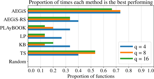
Figure 2: Synthetic function optimisation summary. Bar lengths correspond to the proportion of times that a method is best or statistically equivalent to the best method across the 15 synthetic functions, for $q\in\{4,8,16\}$ workers.

4.2 Hyperparameter Optimisation

Like Souza et al. [2020], we optimise the hyperparameters of three meta-surrogate optimisation tasks corresponding to a SVM, a fully connected neural network (FC-NET) and XGBoost. These are part of the Profet benchmark [Klein et al., 2019, Paleyes et al., 2019] and are drawn from generative models built using performance data on multiple datasets. They aim to mimic the landscape of expensive hyperparameter optimisation tasks, preserving the global landscape characteristics of the modelled methods and giving local variation between function draws from the generative model. This allows far more evaluations to be carried out than would be possible with the modelled problems.

Here, we optimise $51$ instances of each meta-surrogate, repeating the optimisation $N=20$ times per instance with different paired training data for each of the $N$ runs. Details of the construction of each problem are given in the supplementary material. The SVM problem had $2$ parameters; the FC-NET problem $6$; and the XGBoost problem $8$.

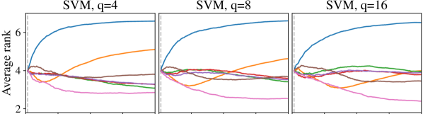
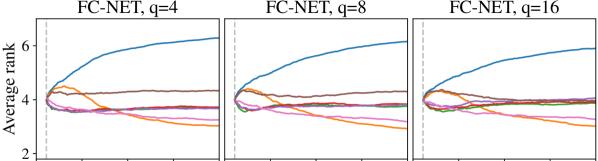
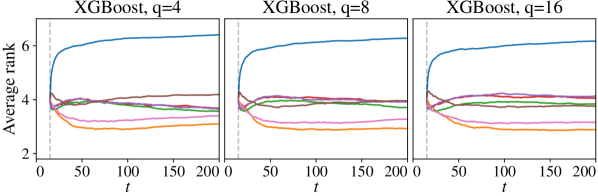
Figure 3: Average ranking scores for the three meta-surrogate benchmarks for $q\in\{4,8,16\}$.

We compare each evaluated method by computing the average ranking score in every iteration for each problem instance. We follow Feurer et al. [2015] and compute this by, for each problem instance, drawing a bootstrap sample of $1000$ runs out of the $7^{N}$ possible combinations and calculating the fractional ranking after each of the $200$ iterations. The ranks are then averaged over all $51$ problem instances.

Figure 3 shows the average ranks of the methods on all three problems for $q\in\{4,8,16\}$. Similarly to the synthetic functions, all three penalisation methods (KB, LB and PLAyBOOK) perform comparably and AEGiS is consistently superior to them after roughly 50 function evaluations. On the FC-NET and XGBoost problems TS performs similarly to AEGiS, and indeed is better on the XGBoost problem. However, AEGiS-RS performs consistently worse, supporting the contention that choosing random locations that lie in the Pareto set is beneficial.

4.3 Active Learning for Robot Pushing

Following Wang and Jegelka [2017] and De Ath et al. [2021], we optimise the control parameters for two instance-based active learning robot pushing problems [Wang et al., 2018]. In push4, a robot pushes an object towards an unknown target location. It receives the object-target distance once it has finished pushing. The location of the robot, the orientation of its pushing hand and for how long it pushes are the parameters to be optimised with the goal of minimising this distance. The push8 problem has two robots that receive the distance between their respective objects and targets after pushing — we minimise the sum of these distances. In both problems the target location(s) are chosen randomly, with the constraint that they cannot overlap. We note that the push8 problem is much more difficult because the robots can block each other, and so each problem instance may not be completely solvable. Further details of the problems are provided in the supplementary material.

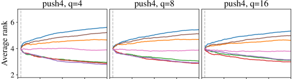
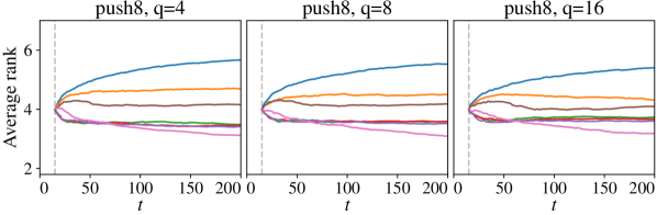
Figure 4: Average ranking scores for the two robot pushing problems for $q\in\{4,8,16\}$.

Average rank score plots, calculated in the same way as described in Section 4.2, are shown in Figure 4. The EI-based methods continue to have very similar performance to one another, and are the best methods on push4, and, even though it is not the best method, AEGiS still out-performs TS consistently. On push8, the EI-based methods initially improve on AEGiS in terms of average rank but then stagnate and are overtaken by AEGiS after roughly 75 function evaluations.

4.4 Additional Experiments

Lastly, we describe an ablation study, experiments on setting the degree of deliberate exploration ($\epsilon=\epsilon_{T}+\epsilon_{P}$), together with the optimal ratio $\epsilon_{T}:\epsilon_{P}$. Finally, we compare AEGiS, EI and TS in the sequential BO setting ($q=1$). See supplementary material for full results.

Ablation Study

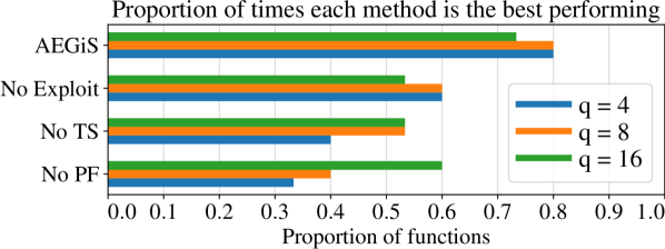
Figure 5: Ablation study summary. The bars correspond to the proportion of times that a method is best or statistically equivalent to the best method across the $15$ synthetic functions, for $q\in\{4,8,16\}$.

Here, we conduct an ablation study on AEGiS using the $15$ synthetic benchmark functions used in Section 4.1. Since AEGiS-RS is consistently outperformed by AEGiS, we omit it from this study. We compare to AEGiS in the following ways: No Exploit, without the exploitation ($\epsilon_{T}=\epsilon_{P}=1/2$); No TS, with no Thompson sampling ($\epsilon_{T}=0;\epsilon_{P}=\epsilon$); No PF, without Pareto set selection ($\epsilon_{T}=\epsilon,\epsilon_{P}=0$). In all cases $\epsilon=\min(2/\sqrt{d},1)$.

Figure 5 shows that all three components combine to give the best results and that removing any of the three results in an inferior algorithm. As can be seen, the removal of either TS or Pareto set selection considerably reduces the performance of the algorithm. Note that the results for No Exploit are inflated because the method is equivalent to AEGiS on the 5 out of the 15 benchmark functions that have $d\leq 4$ dimensions.

Setting $\epsilon$

We investigate the rate at which the degree of deliberate exploitation of the surrogate model’s posterior mean function should increase with problem dimensionality $d$. In AEGiS, exploitation is carried out $1-(\epsilon_{T}+\epsilon_{P})$ proportion of the time. As above we chose $\epsilon_{T}=\epsilon_{P}=\epsilon/2$ and $\epsilon$ was chosen a priori to decay like $1/\sqrt{d}$, i.e. $\epsilon=\min(2/\sqrt{d},1)$. Here, we bracket this decay rate with a quicker decay (more exploitation) and a slower decay (more exploration). Specifically, we evaluate AEGiS on the $15$ synthetic test functions using $\epsilon=\min(2/(d-2),1)$ and $\epsilon=\min(2/\log(d+3),1)$ labelled slower and faster respectively. These decay functions were chosen because they match AEGiS and provide no exploitation when $d\leq 4$, i.e. $\epsilon=0.5$. See the supplementary material for a visual comparison of the rates. Figure 6 summarises the results on the $15$ test functions. When using a smaller number of workers ($q\in\{4,8\}$) the $2/\sqrt{d}$ decay gives superior performance. However, when $q=16$ there is little to differentiate between the three rates. We note that when $d$ is large the faster rate of the decay (more exploitation for a given $d$) is superior; see the supplementary material for full details.

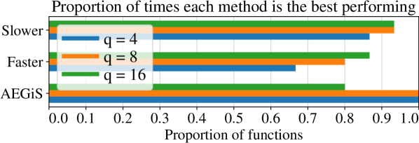
Figure 6: Selecting $\epsilon$: faster and slower correspond to quicker and slower rates of $\epsilon$ decay than AEGiS, resulting in more or less exploitation respectively.

Proportion of TS to PF selection

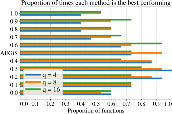
Figure 7: Proportion of TS to Pareto set selection for proportions $\gamma\in\{0,0.1,\dots,1\}$ (vertical axis). Note that the label AEGiS corresponds to $\gamma=0.5$.

In the above evaluations TS and PF were selected with equal probability $\epsilon_{T}=\epsilon_{P}$. Here, we investigate the proportion of times that TS should be chosen over Pareto set selection. Specifically we evaluate AEGiS on the synthetic benchmark functions for $q\in\{4,8,16\}$ with the split between exploitation, TS and Pareto set selection being $1-\epsilon$, $\epsilon_{T}=\gamma\epsilon$ and $\epsilon_{P}=(1-\gamma)\epsilon$ respectively and $\gamma\in\{0,0.1,\dots,1\}$. Note that two of the methods evaluated in the earlier ablation study, No TS and No PF, correspond to $\gamma=0$ and $\gamma=1$ respectively. Figure 7 summarises the results on the 15 synthetic benchmark functions. It shows that using more TS than Pareto set selection appears detrimental to AEGiS, whereas using less TS, i.e. a smaller value of $\gamma$ leads to slightly improved average performance over $0.5$. Interestingly, while AEGiS generally performed better with a smaller value of $\gamma$, for some test functions, e.g. Rosenbrock, larger values were preferred – see the supplementary material for all convergence plots and tabulated results. In general we recommend the standard setting $\epsilon_{T}=\epsilon_{P}=\epsilon/2$.

Sequential BO

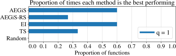
Figure 8: Synthetic function optimisation summary for the sequential setting ($q=1$). Bar lengths correspond to the proportion of times that a method is best or statistically equivalent to the best method across the 15 synthetic functions.

Finally, we evaluate AEGiS in the sequential setting, i.e. with $q=1$. In this setting KB, LP, and PLAyBOOK are equivalent because they all select the next (and only) location to be evaluated using EI. Therefore, we compare AEGiS and AEGiS-RS to TS, EI, and Latin hypercube sampling. As shown in Figure 8, AEGiS and EI had approximately equivalent performance, and they were both superior to AEGiS-RS and TS. This again emphasises the importance of sampling from $\tilde{\mathcal{P}}$. An ablation study was also carried out with similar findings: removing the sampling from $\tilde{\mathcal{P}}$ led to a large reduction in performance. This was a larger drop in performance in comparison to the ablation study using larger values of $q$. We suspect that this is because the model will naturally be of a higher quality at any iteration for $q=1$ and thus selection from $\tilde{\mathcal{P}}$ will be even more informative to the optimisation process. Different rates of $\epsilon$ decay were also investigated as before, and similar results were found: both decreasing and increasing the rate of decay led to worse performance, with the largest decrease coming from increasing the rate and thus increasing exploitation further.

5 Conclusion

Practical optimisation of expensive functions can often make use of parallel hardware to rapidly obtain results. The AEGiS method makes best use of hardware resources through asynchronous Bayesian optimisation by combining greedy exploitation of the surrogate mean prediction with Thompson sampling and exploratory moves from the approximate Pareto set that maximally trades off exploration and exploitation. The ablation study verifies the importance of each of these components. With only a single worker this simple algorithm is no worse than BO using expected improvement. As the problem dimension increases deliberate exploratory moves are less necessary because of the inadvertent exploration due to modelling inaccuracies. We showed empirically on a wide range of problems that setting $\epsilon\propto 2/\sqrt{d}$ is more efficient than faster or slower rates of reducing the amount of exploration carried out as the problem dimensionality $d$ increases.

Unlike other methods, such as PLAyBOOK and Thompson sampling, AEGiS cannot be trivially transformed into a synchronous batch BO method, and therefore it cannot be directly compared to a synchronous version of itself. The closest method in spirit is the $\epsilon$-shotgun method of De Ath et al. [2020]. It scatters $q-1$ samples around a central location, where the samples are distributed according the properties of the surrogate model’s landscape. The central location is chosen to be either the most exploitative location or a randomly selected location from the Pareto set. Interestingly the authors of both PLAyBOOK and Thompson sampling empirically found that, even though there is less information available for the selection of each asynchronous location, their methods outperformed their synchronous counterparts. We note that AEGiS is more effective than both PLAyBOOK and Thompson sampling and, therefore, also their synchronous equivalents.

Although AEGiS is robust to both the amount of exploration ($\epsilon_{T}+\epsilon_{P}$) and the ratio $\epsilon_{T}:\epsilon_{P}$, the combination of greedy exploitation, Thompson sampling and selection from the exploration-exploitation Pareto set is a challenge to obtaining non-trivial bounds on the convergence rate. While future work will concentrate on providing such theoretical guarantees, our extensive empirical evaluation shows that AEGiS is a simple, practical and robust method for asynchronous batch Bayesian optimisation.