1 Introduction
Consider the problem of parameter estimation by n 𝑛 n
independent observations X ( n ) = ( X 1 , … , X n ) superscript 𝑋 𝑛 subscript 𝑋 1 … subscript 𝑋 𝑛 X^{(n)}=\left(X_{1},\ldots,X_{n}\right) . If we suppose
that the density function f ( ϑ , x ) 𝑓 italic-ϑ 𝑥 f\left(\vartheta,x\right) of the observation
X j subscript 𝑋 𝑗 X_{j} is regular , i.e., is sufficiently smooth with respect to parameter
ϑ italic-ϑ \vartheta , then the well-know estimators (MLE, Bayesian estimator, method
of moments estimators) are consistent, asymptotically normal and we have the
convergence of polynomial moments ( p > 0 𝑝 0 p>0 ):
ϑ ¯ n ⟶ ϑ 0 , n ( ϑ ¯ n − ϑ 0 ) ⟹ ξ ∼ 𝒩 ( 0 , D ( ϑ 0 ) 2 ) , formulae-sequence ⟶ subscript ¯ italic-ϑ 𝑛 subscript italic-ϑ 0 ⟹ 𝑛 subscript ¯ italic-ϑ 𝑛 subscript italic-ϑ 0 𝜉 similar-to 𝒩 0 D superscript subscript italic-ϑ 0 2 \displaystyle\bar{\vartheta}_{n}\longrightarrow\vartheta_{0},\qquad\qquad\sqrt{n}\left(\bar{\vartheta}_{n}-\vartheta_{0}\right)\Longrightarrow\xi\sim{\cal N}\left(0,{\rm D}\left(\vartheta_{0}\right)^{2}\right),
lim n → ∞ n p / 2 𝐄 ϑ 0 | ϑ ¯ n − ϑ 0 | p ⟶ D ( ϑ 0 ) p 2 𝐄 | ζ | p , ζ ∼ 𝒩 ( 0 , 1 ) . formulae-sequence ⟶ subscript → 𝑛 superscript 𝑛 𝑝 2 subscript 𝐄 subscript italic-ϑ 0 superscript subscript ¯ italic-ϑ 𝑛 subscript italic-ϑ 0 𝑝 D superscript subscript italic-ϑ 0 𝑝 2 𝐄 superscript 𝜁 𝑝 similar-to 𝜁 𝒩 0 1 \displaystyle\lim_{n\rightarrow\infty}n^{p/2}\mathbf{E}_{\vartheta_{0}}\left|\bar{\vartheta}_{n}-\vartheta_{0}\right|^{p}\longrightarrow{\rm D}\left(\vartheta_{0}\right)^{\frac{p}{2}}\mathbf{E}\left|\zeta\right|^{p},\qquad\zeta\sim{\cal N}\left(0,1\right).
Here we denoted ϑ 0 subscript italic-ϑ 0 \vartheta_{0} the true value and D ( ϑ 0 ) 2 D superscript subscript italic-ϑ 0 2 {\rm D}\left(\vartheta_{0}\right)^{2} is the limit variance of the estimator
ϑ ¯ n subscript ¯ italic-ϑ 𝑛 \bar{\vartheta}_{n} . These relations can be written as follows
ϑ ¯ n − ϑ 0 = o ( 1 ) , subscript ¯ italic-ϑ 𝑛 subscript italic-ϑ 0 𝑜 1 \displaystyle\bar{\vartheta}_{n}-\vartheta_{0}=o\left(1\right),
ϑ ¯ n − ϑ 0 = φ n ξ ( 1 + o ( 1 ) ) , subscript ¯ italic-ϑ 𝑛 subscript italic-ϑ 0 subscript 𝜑 𝑛 𝜉 1 𝑜 1 \displaystyle\bar{\vartheta}_{n}-\vartheta_{0}=\varphi_{n}\xi\left(1+o\left(1\right)\right), (1)
𝐄 ϑ 0 | ϑ ¯ n − ϑ 0 | 2 = φ n 2 D ( ϑ 0 ) 2 ( 1 + o ( 1 ) ) , subscript 𝐄 subscript italic-ϑ 0 superscript subscript ¯ italic-ϑ 𝑛 subscript italic-ϑ 0 2 superscript subscript 𝜑 𝑛 2 D superscript subscript italic-ϑ 0 2 1 𝑜 1 \displaystyle\mathbf{E}_{\vartheta_{0}}\left|\bar{\vartheta}_{n}-\vartheta_{0}\right|^{2}=\varphi_{n}^{2}{\rm D}\left(\vartheta_{0}\right)^{2}\left(1+o\left(1\right)\right), (2)
𝐏 ϑ 0 ( D ( ϑ 0 ) − 1 φ n − 1 ( ϑ ¯ n − ϑ 0 ) < x ) = F ( x ) + o ( 1 ) . subscript 𝐏 subscript italic-ϑ 0 D superscript subscript italic-ϑ 0 1 superscript subscript 𝜑 𝑛 1 subscript ¯ italic-ϑ 𝑛 subscript italic-ϑ 0 𝑥 𝐹 𝑥 𝑜 1 \displaystyle\mathbf{P}_{\vartheta_{0}}\left({\rm D}\left(\vartheta_{0}\right)^{-1}\varphi_{n}^{-1}\left(\bar{\vartheta}_{n}-\vartheta_{0}\right)<x\right)=F\left(x\right)+o\left(1\right). (3)
Here φ n = n − 1 / 2 subscript 𝜑 𝑛 superscript 𝑛 1 2 \varphi_{n}=n^{-1/2} , we take p = 2 𝑝 2 p=2 and F ( x ) 𝐹 𝑥 F\left(x\right) is distribution
function of Gaussian law 𝒩 ( 0 , 1 ) 𝒩 0 1 {\cal N}\left(0,1\right) . Of course, the relation
in ( 1 ) is just a symbolique writing because the limit Gaussian variable
ξ 𝜉 \xi is not defined on the same probability space, we have convergence in
distribution only.
If the volume n 𝑛 n of observations is large, then the relations ( 1 )-( 3 ) describe well
the distribution of the error of estimation. For the
moderate values of n 𝑛 n the real distribution of ϑ ¯ n − ϑ 0 subscript ¯ italic-ϑ 𝑛 subscript italic-ϑ 0 \bar{\vartheta}_{n}-\vartheta_{0} and of the moments 𝐄 ϑ 0 | ϑ ¯ n − ϑ 0 | 2 subscript 𝐄 subscript italic-ϑ 0 superscript subscript ¯ italic-ϑ 𝑛 subscript italic-ϑ 0 2 \mathbf{E}_{\vartheta_{0}}\left|\bar{\vartheta}_{n}-\vartheta_{0}\right|^{2} can be quite far from the given here limit values. The better
approximations for the distribution function and the moments can be obtained
with the help of well-known asymptotic expansion theory. There are at
least three types of expansions:
Stochastic expansion
ϑ ¯ n − ϑ 0 = φ n ξ n , 1 + … + φ n k ξ n , k + o ( φ n k ) , subscript ¯ italic-ϑ 𝑛 subscript italic-ϑ 0 subscript 𝜑 𝑛 subscript 𝜉 𝑛 1
… superscript subscript 𝜑 𝑛 𝑘 subscript 𝜉 𝑛 𝑘
𝑜 superscript subscript 𝜑 𝑛 𝑘 \displaystyle\bar{\vartheta}_{n}-\vartheta_{0}=\varphi_{n}\xi_{n,1}+\ldots+\varphi_{n}^{k}\xi_{n,k}+o\left(\varphi_{n}^{k}\right), (4)
where ξ n , i subscript 𝜉 𝑛 𝑖
\xi_{n,i} are bounded in probability random variables,
Expansion of the moments
𝐄 ϑ | ϑ ¯ n − ϑ 0 | 2 = φ n 2 P n , 1 + … + φ n 2 k P n , k + o ( φ n k ) , subscript 𝐄 italic-ϑ superscript subscript ¯ italic-ϑ 𝑛 subscript italic-ϑ 0 2 superscript subscript 𝜑 𝑛 2 subscript 𝑃 𝑛 1
… superscript subscript 𝜑 𝑛 2 𝑘 subscript 𝑃 𝑛 𝑘
𝑜 superscript subscript 𝜑 𝑛 𝑘 \displaystyle\mathbf{E}_{\vartheta}\left|\bar{\vartheta}_{n}-\vartheta_{0}\right|^{2}=\varphi_{n}^{2}P_{n,1}+\ldots+\varphi_{n}^{2k}P_{n,k}+o\left(\varphi_{n}^{k}\right), (5)
where P n , i subscript 𝑃 𝑛 𝑖
P_{n,i} are some bounded real values,
Expansion of the distribution function
𝐏 ϑ 0 ( ϑ ¯ n − ϑ 0 D ( ϑ 0 ) n < x ) = F ( x ) + φ n p 1 ( x ) + … + φ n k p k ( x ) + o ( φ n k ) , subscript 𝐏 subscript italic-ϑ 0 subscript ¯ italic-ϑ 𝑛 subscript italic-ϑ 0 D subscript italic-ϑ 0 𝑛 𝑥 𝐹 𝑥 subscript 𝜑 𝑛 subscript 𝑝 1 𝑥 … superscript subscript 𝜑 𝑛 𝑘 subscript 𝑝 𝑘 𝑥 𝑜 superscript subscript 𝜑 𝑛 𝑘 \displaystyle\mathbf{P}_{\vartheta_{0}}\left(\frac{\bar{\vartheta}_{n}-\vartheta_{0}}{{\rm D}\left(\vartheta_{0}\right)\sqrt{n}}<x\right)=F\left(x\right)+\varphi_{n}p_{1}\left(x\right)+\ldots+\varphi_{n}^{k}p_{k}\left(x\right)+o\left(\varphi_{n}^{k}\right), (6)
where p i ( x ) subscript 𝑝 𝑖 𝑥 p_{i}\left(x\right) are some products of polynomials
and f ( x ) 𝑓 𝑥 f\left(x\right) (density function of 𝒩 ( 0 , 1 ) 𝒩 0 1 {\cal N}\left(0,1\right) ). The value of the parameter k 𝑘 k depends on the
smoothness of the model with respect to unknown paramater.
We can mention here the works devoted to asymptotic expansions of estimators
for independent identically distributed observations of the random variables
[ 2 ] , [ 6 ] , [ 7 ] , [ 8 ] , [ 10 ] , [ 11 ] ,
[ 16 ] , [ 17 ] , [ 18 ] . In the last book there is an extensive
list of references. Such asymptotic expansions are widely used in bootstrap
too [ 1 ] . The difference between these works is in the conditions
of regularity and in the estimates of the residuals o ( ⋅ ) 𝑜 ⋅ o\left(\cdot\right) in
( 4 )-( 6 ).
Note that in the majority of these works the results are asymptotic in
nature , i.e., the residuals in expansions ( 3 )-( 5 ) are of the type o ( φ n k ) 𝑜 superscript subscript 𝜑 𝑛 𝑘 o\left(\varphi_{n}^{k}\right) or φ n k + δ o ( 1 ) , δ ∈ ( 0 , 1 ) superscript subscript 𝜑 𝑛 𝑘 𝛿 𝑜 1 𝛿
0 1 \varphi_{n}^{k+\delta}o\left(1\right),\delta\in\left(0,1\right) , where o ( 1 ) → 0 → 𝑜 1 0 o\left(1\right)\rightarrow 0 as n → ∞ → 𝑛 n\rightarrow\infty and nothing can be said about the term
o ( 1 ) 𝑜 1 o\left(1\right) for finite n 𝑛 n .
The expansions of the errors of estimation by the powers of small parameters
in the case of observations of continuous time stochastic processes were
obtained in the works [ 4 ] (signal in white Gaussian noise),
[ 12 ] , [ 15 ] (inhomogeneous Poisson processes),
[ 13 ] , [ 19 ] , [ 20 ] , [ 14 ] , (diffusion processes),
[ 21 ] (martingales with jumps).
One of the goals of this work is to obtain such expansions (stochastic,
moments and distribution function) for the recently introduced class of
estimators: method of moments estimators (MME) in the case of
observations of inhomogeneous Poisson processes. The method of moments allowed
to have explicit expressions for many models with intensity functions non
linearly depending on the unknown parameters, where the traditional MLE have
no explicit expressions and therefore MME provides essential gain in the
calculation of the consistent and asymptotically normal estimators. Note that
the MME are used in One-step MLE construction to obtain the asymptotically
efficient estimators too [ 9 ] .
It is known that the publications
related with the asymptotic expansions ( 4 )-( 6 ) in statistics are
technically quite cumbersome (see, e.g., [ 18 ] and references
therein). In the considered in this work case the exposition is essentially
simplified because the random variables ξ n , i subscript 𝜉 𝑛 𝑖
\xi_{n,i} in ( 4 ) have the
form ξ n , i = η n i subscript 𝜉 𝑛 𝑖
superscript subscript 𝜂 𝑛 𝑖 \xi_{n,i}=\eta_{n}^{i} with the same η n subscript 𝜂 𝑛 \eta_{n} . Another advantage of this
work with respect to traditional asymptotic expansions is the using in
obtaining all expansions of the method of good sets , which in reality
allows to obtain non asymptotic expansions . This method was developed by
Burnashev in [ 4 ] and [ 6 ] . His approach allows to have
expansions ( 4 ) and ( 5 ) non asymptotic in nature . This means,
that the residuals in ( 4 ) and ( 5 ) for finite n 𝑛 n can be estimated
from above and from below with known rates and constants. Remark that this
method was already applied to obtain non asymptotic expansions in the works
[ 12 ] , [ 13 ] , [ 14 ] , [ 15 ] .
2 Method of Moments Estimator
Let us consider the following problem of parameter estimation. Suppose that we
have n 𝑛 n independent observations of inhomogeneous Poisson processes
X ( n ) = ( X 1 , … , X n ) superscript 𝑋 𝑛 subscript 𝑋 1 … subscript 𝑋 𝑛 X^{(n)}=\left(X_{1},\ldots,X_{n}\right) , where X j = { X j ( t ) , t ∈ 𝒯 } subscript 𝑋 𝑗 subscript 𝑋 𝑗 𝑡 𝑡
𝒯 X_{j}\!=\!\bigl{\{}X_{j}(t),\,t\in{\cal T}\bigr{\}} with intensity function
λ ( ϑ , t ) , t ∈ 𝒯 𝜆 italic-ϑ 𝑡 𝑡
𝒯 \lambda\left(\vartheta,t\right),t\in{\cal T} . Here 𝒯 ⊂ ℛ 𝒯 ℛ {\cal T}\subset{\cal R} is some interval. It can be 𝒯 = [ 0 , τ ] 𝒯 0 𝜏 {\cal T}=\left[0,\tau\right] , 𝒯 = [ 0 , + ∞ ) 𝒯 0 {\cal T}=[0,+\infty) , 𝒯 = ℛ 𝒯 ℛ {\cal T}={\cal R} or any other interval on the
line. As usual, X j ( ⋅ ) subscript 𝑋 𝑗 ⋅ X_{j}\left(\cdot\right) are counting processes (see details
in [ 15 ] ). We have to estimate the parameter ϑ ∈ Θ = ( α , β ) italic-ϑ Θ 𝛼 𝛽 \vartheta\in\Theta=\left(\alpha,\beta\right) by the observations X ( n ) superscript 𝑋 𝑛 X^{\left(n\right)} and
to describe the properties of estimators in the asymptotic of large samples
( n → ∞ → 𝑛 n\rightarrow\infty ).
For the study we take the method of moments estimator (MME) defined as
follows. Introduce the functions g ( t ) , t ∈ 𝒯 𝑔 𝑡 𝑡
𝒯 g(t),t\in{\cal T} and the functions
m ( ϑ ) = ∫ 𝒯 g ( t ) λ ( ϑ , t ) d t , ϑ ∈ Θ and m ¯ n = 1 n ∑ j = 1 n ∫ 𝒯 g ( t ) d X j ( t ) . formulae-sequence 𝑚 italic-ϑ subscript 𝒯 𝑔 𝑡 𝜆 italic-ϑ 𝑡 differential-d 𝑡 italic-ϑ Θ and subscript ¯ 𝑚 𝑛 1 𝑛 superscript subscript 𝑗 1 𝑛 subscript 𝒯 𝑔 𝑡 differential-d subscript 𝑋 𝑗 𝑡 m(\vartheta)=\int_{\cal T}g(t)\lambda(\vartheta,t){\rm d}t,\quad\vartheta\in\Theta\quad\mbox{and}\quad\bar{m}_{n}=\frac{1}{n}\sum_{j=1}^{n}\int_{\cal T}g(t){\rm d}X_{j}(t).
We suppose that we have such functions λ ( ϑ , t ) , ϑ ∈ Θ , t ∈ 𝒯 , formulae-sequence 𝜆 italic-ϑ 𝑡 italic-ϑ
Θ 𝑡 𝒯 \lambda\left(\vartheta,t\right),\vartheta\in\Theta,t\in{\cal T},
and g ( t ) 𝑔 𝑡 g\left(t\right) that the function m ( ϑ ) , α ≤ ϑ ≤ β 𝑚 italic-ϑ 𝛼
italic-ϑ 𝛽 m\left(\vartheta\right),\alpha\leq\vartheta\leq\beta is monotone. Without loss of generality we assume that
it is monotone increasing.
Let us introduce the following notations:
ℳ = { m ( ϑ ) : ϑ ∈ [ α , β ] } = [ m ( α ) , m ( β ) ] ℳ conditional-set 𝑚 italic-ϑ italic-ϑ 𝛼 𝛽 𝑚 𝛼 𝑚 𝛽 \displaystyle{\cal M}=\left\{m\left(\vartheta\right):\;\vartheta\in\left[\alpha,\beta\right]\right\}=\left[m\left(\alpha\right),m\left(\beta\right)\right]
For y ∈ ℳ 𝑦 ℳ y\in{\cal M} we write the solution of the equation m ( ϑ ) = y 𝑚 italic-ϑ 𝑦 m(\vartheta)=y as
ϑ = m − 1 ( y ) = G ( y ) italic-ϑ superscript 𝑚 1 𝑦 𝐺 𝑦 \vartheta=m^{-1}(y)=G(y) . Therefore the function G ( y ) 𝐺 𝑦 G(y) is inverse
for m ( ϑ ) 𝑚 italic-ϑ m(\vartheta) and G ( m ( ϑ ) ) = ϑ 𝐺 𝑚 italic-ϑ italic-ϑ G(m(\vartheta))=\vartheta .
We define the method of moments estimator (MME) ϑ ˇ n subscript ˇ italic-ϑ 𝑛 \check{\vartheta}_{n}
by the following equation
ϑ ˇ n = arg inf ϑ ∈ Θ ( m ( ϑ ) − m ¯ n ) 2 . subscript ˇ italic-ϑ 𝑛 subscript infimum italic-ϑ Θ superscript 𝑚 italic-ϑ subscript ¯ 𝑚 𝑛 2 \check{\vartheta}_{n}=\arg\inf_{\vartheta\in\Theta}\left(m(\vartheta)-\bar{m}_{n}\right)^{2}.
This estimator admits the representation
ϑ ˇ n = α 1I { m ¯ n ≤ m ( α ) } + ϑ ¯ n 1I { m ( α ) < m ¯ n < m ( β ) } + β 1I { m ¯ n ≥ m ( β ) } , subscript ˇ italic-ϑ 𝑛 𝛼 subscript 1I subscript ¯ 𝑚 𝑛 𝑚 𝛼 subscript ¯ italic-ϑ 𝑛 subscript 1I 𝑚 𝛼 subscript ¯ 𝑚 𝑛 𝑚 𝛽 𝛽 subscript 1I subscript ¯ 𝑚 𝑛 𝑚 𝛽 \displaystyle\check{\vartheta}_{n}=\alpha\mbox{1I}_{\left\{\bar{m}_{n}\leq m(\alpha)\right\}}+\bar{\vartheta}_{n}\mbox{1I}_{\left\{m(\alpha)<\bar{m}_{n}<m(\beta)\right\}}+\beta\mbox{1I}_{\left\{\bar{m}_{n}\geq m(\beta)\right\}}, (7)
where ϑ ¯ n subscript ¯ italic-ϑ 𝑛 \bar{\vartheta}_{n} is a solution of the equation m ( ϑ ¯ n ) = m ¯ n 𝑚 subscript ¯ italic-ϑ 𝑛 subscript ¯ 𝑚 𝑛 m(\bar{\vartheta}_{n})=\bar{m}_{n}
when m ¯ n ∈ ( m ( α ) , m ( β ) ) subscript ¯ 𝑚 𝑛 𝑚 𝛼 𝑚 𝛽 \bar{m}_{n}\in\left(m(\alpha),m(\beta)\right) . The value
ϑ ˇ n = α subscript ˇ italic-ϑ 𝑛 𝛼 \check{\vartheta}_{n}=\alpha (respectively
ϑ ˇ n = β subscript ˇ italic-ϑ 𝑛 𝛽 \check{\vartheta}_{n}=\beta ) corresponds to m ≤ m ( α ) 𝑚 𝑚 𝛼 m\leq m(\alpha) closest to
m ¯ n subscript ¯ 𝑚 𝑛 \bar{m}_{n} (respectively m ≥ m ( β ) 𝑚 𝑚 𝛽 m\geq m(\beta) closest to m ¯ n subscript ¯ 𝑚 𝑛 \bar{m}_{n} ). Recall
that with probability p n = exp ( − n Λ ( 𝒯 ) ) subscript 𝑝 𝑛 𝑛 Λ 𝒯 p_{n}=\exp\left(-n\Lambda\left({\cal T}\right)\right)
we have no events (jumps) in all observations. Here
Λ ( 𝒯 ) = ∫ 𝒯 λ ( ϑ , t ) d t . Λ 𝒯 subscript 𝒯 𝜆 italic-ϑ 𝑡 differential-d 𝑡 \Lambda\left({\cal T}\right)=\int_{{\cal T}}\lambda\left(\vartheta,t\right){\rm d}t.
This estimator was recently studied in [ 9 ] . It was shown that as
n → ∞ → 𝑛 n\rightarrow\infty and under mild regularity conditions this estimator is
consistent
ϑ ˇ n ⟶ ϑ 0 ⟶ subscript ˇ italic-ϑ 𝑛 subscript italic-ϑ 0 \displaystyle\check{\vartheta}_{n}\longrightarrow\vartheta_{0} (8)
(here and in the sequel ϑ 0 subscript italic-ϑ 0 \vartheta_{0} denotes the true value), asymptotically
normal
n ( ϑ ˇ n − ϑ 0 ) ⟹ 𝒩 ( 0 , D ( ϑ 0 ) 2 ) ⟹ 𝑛 subscript ˇ italic-ϑ 𝑛 subscript italic-ϑ 0 𝒩 0 D superscript subscript italic-ϑ 0 2 \displaystyle\sqrt{n}\left(\check{\vartheta}_{n}-\vartheta_{0}\right)\Longrightarrow{\cal N}\left(0,{\rm D}\left(\vartheta_{0}\right)^{2}\right) (9)
or, for any x ∈ ℛ 𝑥 ℛ x\in{\cal R}
𝐏 ϑ 0 ( D ( ϑ 0 ) − 1 n ( ϑ ˇ n − ϑ 0 ) < x ) ⟶ F ( x ) = 1 2 π ∫ − ∞ x e − y 2 2 d y . ⟶ subscript 𝐏 subscript italic-ϑ 0 D superscript subscript italic-ϑ 0 1 𝑛 subscript ˇ italic-ϑ 𝑛 subscript italic-ϑ 0 𝑥 𝐹 𝑥 1 2 𝜋 superscript subscript 𝑥 superscript 𝑒 superscript 𝑦 2 2 differential-d 𝑦 \displaystyle\mathbf{P}_{\vartheta_{0}}\left({\rm D}\left(\vartheta_{0}\right)^{-1}\sqrt{n}\left(\check{\vartheta}_{n}-\vartheta_{0}\right)<x\right)\longrightarrow F\left(x\right)=\frac{1}{\sqrt{2\pi}}\int_{-\infty}^{x}e^{-\frac{y^{2}}{2}}{\rm d}y.
We have as well the convergence of all polynomial moments: for any p > 0 𝑝 0 p>0
n p 2 𝐄 ϑ 0 | ϑ ˇ n − ϑ 0 | p ⟶ 𝐄 | ζ | p D ( ϑ 0 ) p 2 , ζ ∼ 𝒩 ( 0 , 1 ) . formulae-sequence ⟶ superscript 𝑛 𝑝 2 subscript 𝐄 subscript italic-ϑ 0 superscript subscript ˇ italic-ϑ 𝑛 subscript italic-ϑ 0 𝑝 𝐄 superscript 𝜁 𝑝 D superscript subscript italic-ϑ 0 𝑝 2 similar-to 𝜁 𝒩 0 1 \displaystyle n^{\frac{p}{2}}\mathbf{E}_{\vartheta_{0}}\left|\check{\vartheta}_{n}-\vartheta_{0}\right|^{p}\longrightarrow\mathbf{E}\left|\zeta\right|^{p}\;{\rm D}\left(\vartheta_{0}\right)^{\frac{p}{2}},\qquad\zeta\sim{\cal N}\left(0,1\right). (10)
The advantage of the MME can be illustrated with the help of the following examples.
Example 1
Suppose that we have an inhomogeneous Poisson process
X T = ( X t , 0 ≤ t ≤ T ) superscript 𝑋 𝑇 subscript 𝑋 𝑡 0
𝑡 𝑇 X^{T}=\left(X_{t},0\leq t\leq T\right) with τ 𝜏 \tau -periodic intensiy
function λ ( ϑ , t ) , 0 ≤ t ≤ T 𝜆 italic-ϑ 𝑡 0
𝑡 𝑇 \lambda\left(\vartheta,t\right),0\leq t\leq T , i.e., λ ( ϑ , t + k τ ) = λ ( ϑ , t ) 𝜆 italic-ϑ 𝑡 𝑘 𝜏 𝜆 italic-ϑ 𝑡 \lambda\left(\vartheta,t+k\tau\right)=\lambda\left(\vartheta,t\right) for
any k = 1 , 2 , … 𝑘 1 2 …
k=1,2,\ldots . Suppose that
T = n τ 𝑇 𝑛 𝜏 T=n\tau and introduce the independent Poisson processes
X j ( t ) = X ( j − 1 ) τ + t − X ( j − 1 ) τ , t ∈ 𝒯 = [ 0 , τ ] , j = 1 , … , n . formulae-sequence formulae-sequence subscript 𝑋 𝑗 𝑡 subscript 𝑋 𝑗 1 𝜏 𝑡 subscript 𝑋 𝑗 1 𝜏 𝑡 𝒯 0 𝜏 𝑗 1 … 𝑛
\displaystyle X_{j}\left(t\right)=X_{\left(j-1\right)\tau+t}-X_{\left(j-1\right)\tau},\quad t\in{\cal T}=\left[0,\tau\right],\quad j=1,\ldots,n.
Therefore we obtain the observations
X ( n ) = ( X 1 , … , X n ) superscript 𝑋 𝑛 subscript 𝑋 1 … subscript 𝑋 𝑛 X^{\left(n\right)}=\left(X_{1},\ldots,X_{n}\right) with intensity function
λ ( ϑ , t ) 𝜆 italic-ϑ 𝑡 \lambda\left(\vartheta,t\right) and can
construct the MME ϑ ˇ n subscript ˇ italic-ϑ 𝑛 \check{\vartheta}_{n} .
Suppose that we observe a τ 𝜏 \tau -periodic Poisson
signal of intensity function
S ( ϑ , t ) = ϑ h ( t ) 𝑆 italic-ϑ 𝑡 italic-ϑ ℎ 𝑡 S\left(\vartheta,t\right)=\vartheta h\left(t\right) (amplitude modulation)
in the presence of the Poisson noise
of intensity λ 0 > 0 subscript 𝜆 0 0 \lambda_{0}>0 , i.e., we have
λ ( ϑ , t ) = ϑ h ( t ) + λ 0 , 0 ≤ t ≤ τ . formulae-sequence 𝜆 italic-ϑ 𝑡 italic-ϑ ℎ 𝑡 subscript 𝜆 0 0 𝑡 𝜏 \displaystyle\lambda\left(\vartheta,t\right)=\vartheta h\left(t\right)+\lambda_{0},\qquad 0\leq t\leq\tau. (11)
Here h ( ⋅ ) ℎ ⋅ h\left(\cdot\right) is τ 𝜏 \tau -periodic known positive function and
λ 0 > 0 subscript 𝜆 0 0 \lambda_{0}>0 . Remind that the MLE ϑ ^ n subscript ^ italic-ϑ 𝑛 \hat{\vartheta}_{n} for this model has no
explicit representation and is given as solution of the following equation
∑ j = 1 n ∫ 0 τ h ( t ) ϑ ^ n h ( t ) + λ 0 d X j ( t ) = n ∫ 0 τ h ( t ) d t . superscript subscript 𝑗 1 𝑛 superscript subscript 0 𝜏 ℎ 𝑡 subscript ^ italic-ϑ 𝑛 ℎ 𝑡 subscript 𝜆 0 differential-d subscript 𝑋 𝑗 𝑡 𝑛 superscript subscript 0 𝜏 ℎ 𝑡 differential-d 𝑡 \displaystyle\sum_{j=1}^{n}\int_{0}^{\tau}\frac{h\left(t\right)}{\hat{\vartheta}_{n}h\left(t\right)+\lambda_{0}}{\rm d}X_{j}\left(t\right)=n\int_{0}^{\tau}h\left(t\right){\rm d}t.
Despite the numerical difficulties of its calculation there is as well the
problem of definition of this stochastic integral. The calculation of the MME
has no such difficulties and for the wide class of functions g ( ⋅ ) 𝑔 ⋅ g\left(\cdot\right) (say, positive) we have
m ( ϑ ) = ϑ H g + λ 0 G , H g = ∫ 0 τ g ( t ) h ( t ) d t , G = ∫ 0 τ g ( t ) d t formulae-sequence 𝑚 italic-ϑ italic-ϑ subscript 𝐻 𝑔 subscript 𝜆 0 𝐺 formulae-sequence subscript 𝐻 𝑔 superscript subscript 0 𝜏 𝑔 𝑡 ℎ 𝑡 differential-d 𝑡 𝐺 superscript subscript 0 𝜏 𝑔 𝑡 differential-d 𝑡 \displaystyle m\left(\vartheta\right)=\vartheta H_{g}+\lambda_{0}G,\qquad H_{g}=\int_{0}^{\tau}g\left(t\right)h\left(t\right){\rm d}t,\quad G=\int_{0}^{\tau}g\left(t\right){\rm d}t
and ϑ = H g − 1 [ m ( ϑ ) − λ 0 G ] italic-ϑ superscript subscript 𝐻 𝑔 1 delimited-[] 𝑚 italic-ϑ subscript 𝜆 0 𝐺 \vartheta=H_{g}^{-1}\left[m\left(\vartheta\right)-\lambda_{0}G\right] . Hence G ( y ) = H g − 1 [ y − λ 0 G ] 𝐺 𝑦 superscript subscript 𝐻 𝑔 1 delimited-[] 𝑦 subscript 𝜆 0 𝐺 G\left(y\right)=H_{g}^{-1}\left[y-\lambda_{0}G\right] .
The MME
ϑ ˇ n = ( ∫ 0 τ g ( t ) h ( t ) d t ) − 1 [ 1 n ∑ j = 1 n ∫ 0 τ g ( t ) d X j ( t ) − λ 0 ∫ 0 τ g ( t ) d t ] subscript ˇ italic-ϑ 𝑛 superscript superscript subscript 0 𝜏 𝑔 𝑡 ℎ 𝑡 differential-d 𝑡 1 delimited-[] 1 𝑛 superscript subscript 𝑗 1 𝑛 superscript subscript 0 𝜏 𝑔 𝑡 differential-d subscript 𝑋 𝑗 𝑡 subscript 𝜆 0 superscript subscript 0 𝜏 𝑔 𝑡 differential-d 𝑡 \displaystyle\check{\vartheta}_{n}=\left(\int_{0}^{\tau}g\left(t\right)h\left(t\right){\rm d}t\right)^{-1}\left[\frac{1}{n}\sum_{j=1}^{n}\int_{0}^{\tau}g\left(t\right){\rm d}X_{j}\left(t\right)-\lambda_{0}\int_{0}^{\tau}g\left(t\right){\rm d}t\right] (12)
This estimator has the mentioned above properties ( 8 )-( 10 ) (see
[ 9 ] ).
Example 2
. Suppose that the intensity function of the observed
Poisson processes X ( n ) = ( X 1 , … , X n ) superscript 𝑋 𝑛 subscript 𝑋 1 … subscript 𝑋 𝑛 X^{\left(n\right)}=\left(X_{1},\ldots,X_{n}\right) ,
X j = ( X j ( t ) , t ∈ 𝒯 = [ 0 , + ∞ ) ) subscript 𝑋 𝑗 subscript 𝑋 𝑗 𝑡 𝑡
𝒯 0 X_{j}=\left(X_{j}\left(t\right),t\in{\cal T}=[0,+\infty)\right) is
λ ( ϑ , t ) = f ( t ) e − ϑ h ( t ) + q ( t ) , t ≥ 0 . formulae-sequence 𝜆 italic-ϑ 𝑡 𝑓 𝑡 superscript 𝑒 italic-ϑ ℎ 𝑡 𝑞 𝑡 𝑡 0 \displaystyle\lambda\left(\vartheta,t\right)=f\left(t\right)\;e^{-\vartheta h\left(t\right)}+q\left(t\right),\quad t\geq 0. (13)
Here f ( ⋅ ) > 0 , h ( ⋅ ) ≥ 0 formulae-sequence 𝑓 ⋅ 0 ℎ ⋅ 0 f\left(\cdot\right)>0,h\left(\cdot\right)\geq 0 and q ( ⋅ ) ≥ 0 𝑞 ⋅ 0 q\left(\cdot\right)\geq 0
are known
functions, h ( 0 ) = 0 , h ( ∞ ) = ∞ formulae-sequence ℎ 0 0 ℎ h\left(0\right)=0,h\left(\infty\right)=\infty and h ( ⋅ ) ℎ ⋅ h\left(\cdot\right) has continuous derivative h ′ ( ⋅ ) superscript ℎ ′ ⋅ h^{\prime}\left(\cdot\right) . For example,
f ( t ) = 1 + t 4 , h ( t ) = t 2 , q ( t ) = 1 formulae-sequence 𝑓 𝑡 1 superscript 𝑡 4 formulae-sequence ℎ 𝑡 superscript 𝑡 2 𝑞 𝑡 1 f\left(t\right)=1+t^{4},h\left(t\right)=t^{2},q\left(t\right)=1 .
We have to estimate ϑ ∈ ( α , β ) italic-ϑ 𝛼 𝛽 \vartheta\in\left(\alpha,\beta\right) , 0 < α < β < ∞ 0 𝛼 𝛽 0<\alpha<\beta<\infty . Recall
that the MLE has no explicit expression. Let us put
g ( t ) = f ( t ) − 1 h ′ ( t ) 𝑔 𝑡 𝑓 superscript 𝑡 1 superscript ℎ ′ 𝑡 g\left(t\right)=f\left(t\right)^{-1}h^{\prime}\left(t\right) , then
we have
m ( ϑ ) = ∫ 0 ∞ g ( t ) λ ( ϑ , t ) d t = 1 ϑ + R , R = ∫ 0 ∞ h ′ ( t ) q ( t ) f ( t ) d t , formulae-sequence 𝑚 italic-ϑ superscript subscript 0 𝑔 𝑡 𝜆 italic-ϑ 𝑡 differential-d 𝑡 1 italic-ϑ 𝑅 𝑅 superscript subscript 0 superscript ℎ ′ 𝑡 𝑞 𝑡 𝑓 𝑡 differential-d 𝑡 \displaystyle m\left(\vartheta\right)=\int_{0}^{\infty}g\left(t\right)\lambda\left(\vartheta,t\right){\rm d}t=\frac{1}{\vartheta}+R,\quad R=\int_{0}^{\infty}\frac{h^{\prime}\left(t\right)q\left(t\right)}{f\left(t\right)}{\rm d}t,\quad
hence ϑ = ( m ( ϑ ) − R ) − 1 italic-ϑ superscript 𝑚 italic-ϑ 𝑅 1 \vartheta=\left(m\left(\vartheta\right)-R\right)^{-1} and the MME
ϑ ˇ n = ( 1 n ∑ j = 1 n ∫ 0 ∞ h ′ ( t ) f ( t ) d X j ( t ) − R ) − 1 . subscript ˇ italic-ϑ 𝑛 superscript 1 𝑛 superscript subscript 𝑗 1 𝑛 superscript subscript 0 superscript ℎ ′ 𝑡 𝑓 𝑡 differential-d subscript 𝑋 𝑗 𝑡 𝑅 1 \displaystyle\check{\vartheta}_{n}=\left(\frac{1}{n}\sum_{j=1}^{n}\int_{0}^{\infty}\frac{h^{\prime}\left(t\right)}{f\left(t\right)}{\rm d}X_{j}\left(t\right)-R\right)^{-1}.
If we suppose that the corresponding integrals are finite then once more this
estimator has the mentioned above properties ( 8 )-( 10 ) (see
[ 9 ] ).
The case h ( 0 ) ≠ 0 ℎ 0 0 h\left(0\right)\not=0 can be treated by a similar way, but to
define the MME we have to solve the equation
ϑ − 1 e − ϑ h ( 0 ) = y + R , ϑ ∈ Θ . formulae-sequence superscript italic-ϑ 1 superscript 𝑒 italic-ϑ ℎ 0 𝑦 𝑅 italic-ϑ Θ \displaystyle\vartheta^{-1}e^{-\vartheta h\left(0\right)}=y+R,\qquad\vartheta\in\Theta.
Of course, all derivatives of the solution ϑ = G ( y ) italic-ϑ 𝐺 𝑦 \vartheta=G\left(y\right) can be
calculated without problems.
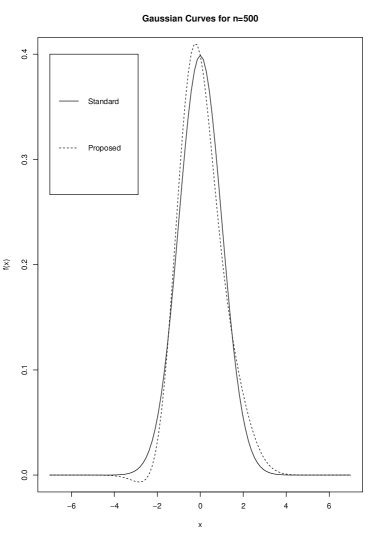
Example 3
Consider Poisson processes
X ( n ) = ( X 1 , … , X n ) superscript 𝑋 𝑛 subscript 𝑋 1 … subscript 𝑋 𝑛 X^{\left(n\right)}=\left(X_{1},\ldots,X_{n}\right) with “Gaussian” intensity
function
λ ( ϑ , t ) = a e − ( t − b ) 2 2 ϑ 2 , t ∈ ℛ . formulae-sequence 𝜆 italic-ϑ 𝑡 𝑎 superscript 𝑒 superscript 𝑡 𝑏 2 2 superscript italic-ϑ 2 𝑡 ℛ \displaystyle\lambda\left(\vartheta,t\right)=a\;e^{-\frac{\left(t-b\right)^{2}}{2\vartheta^{2}}},\quad t\in{\cal R}. (14)
Here a > 0 , b 𝑎 0 𝑏
a>0,b are supposed to be known and we have to estimate ϑ ∈ ( α , β ) italic-ϑ 𝛼 𝛽 \vartheta\in\left(\alpha,\beta\right) , α > 0 𝛼 0 \alpha>0 . Let us take
g 1 ( t ) = ( t − b ) 2 subscript 𝑔 1 𝑡 superscript 𝑡 𝑏 2 g_{1}\left(t\right)=\left(t-b\right)^{2} . Then
m 1 ( ϑ ) = ∫ ℛ ( t − b ) 2 λ ( ϑ , t ) d t = ϑ 3 a 2 π , ϑ = ( m ( ϑ ) a 2 π ) 1 / 3 formulae-sequence subscript 𝑚 1 italic-ϑ subscript ℛ superscript 𝑡 𝑏 2 𝜆 italic-ϑ 𝑡 differential-d 𝑡 superscript italic-ϑ 3 𝑎 2 𝜋 italic-ϑ superscript 𝑚 italic-ϑ 𝑎 2 𝜋 1 3 \displaystyle m_{1}\left(\vartheta\right)=\int_{\cal R}\left(t-b\right)^{2}\lambda\left(\vartheta,t\right){\rm d}t=\vartheta^{3}a\sqrt{2\pi},\qquad\vartheta=\left(\frac{m\left(\vartheta\right)}{a\sqrt{2\pi}}\right)^{1/3}
and
ϑ ˇ n = ( 1 a n 2 π ∑ j = 1 n ∫ ℛ ( t − b ) 2 d X j ( t ) ) 1 / 3 . subscript ˇ italic-ϑ 𝑛 superscript 1 𝑎 𝑛 2 𝜋 superscript subscript 𝑗 1 𝑛 subscript ℛ superscript 𝑡 𝑏 2 differential-d subscript 𝑋 𝑗 𝑡 1 3 \displaystyle\check{\vartheta}_{n}=\left(\frac{1}{an\sqrt{2\pi}}\sum_{j=1}^{n}\int_{\cal R}\left(t-b\right)^{2}{\rm d}X_{j}\left(t\right)\right)^{1/3}.
Another possibility is to take g 2 ( t ) = | t − b | subscript 𝑔 2 𝑡 𝑡 𝑏 g_{2}\left(t\right)=\left|t-b\right| . Then
we obtain m 2 ( ϑ ) = 2 a ϑ 2 subscript 𝑚 2 italic-ϑ 2 𝑎 superscript italic-ϑ 2 m_{2}\left(\vartheta\right)=2a\vartheta^{2} and
ϑ ˇ n = ( 1 2 a n ∑ j = 1 n ∫ ℛ | t − b | d X j ( t ) ) 1 / 2 . subscript ˇ italic-ϑ 𝑛 superscript 1 2 𝑎 𝑛 superscript subscript 𝑗 1 𝑛 subscript ℛ 𝑡 𝑏 differential-d subscript 𝑋 𝑗 𝑡 1 2 \displaystyle\check{\vartheta}_{n}=\left(\frac{1}{2an}\sum_{j=1}^{n}\int_{\cal R}\left|t-b\right|{\rm d}X_{j}\left(t\right)\right)^{1/2}.
The both estimators are consistent and asymptotically normal.
3 Stochastic expansion
The properties ( 9 ), ( 10 ) of the MME ϑ ˇ n subscript ˇ italic-ϑ 𝑛 \check{\vartheta}_{n} can
be written as ( 1 ), ( 2 ) and our goal is to obtain the expansions like
( 4 ) for these estimators too.
Recall, we have n 𝑛 n independent observations of inhomogeneous Poisson
processes X ( n ) superscript 𝑋 𝑛 X^{\left(n\right)} of the same intensity function λ ( ϑ , t ) , t ∈ 𝒯 𝜆 italic-ϑ 𝑡 𝑡
𝒯 \lambda\left(\vartheta,t\right),t\in{\cal T} , where ϑ ∈ Θ = ( α , β ) italic-ϑ Θ 𝛼 𝛽 \vartheta\in\Theta=\left(\alpha,\beta\right) . To estimate ϑ italic-ϑ \vartheta we use the MME
ϑ ˇ n subscript ˇ italic-ϑ 𝑛 \check{\vartheta}_{n} defined in ( 7 ) with some function
g ( ⋅ ) 𝑔 ⋅ g\left(\cdot\right) .
Introduce the notation:
ψ l ( ϑ 0 ) subscript 𝜓 𝑙 subscript italic-ϑ 0 \displaystyle\psi_{l}\left(\vartheta_{0}\right) = G ( l ) ( m ( ϑ 0 ) ) l ! , l = 1 , … , k , π n ( t ) = ∑ j = 1 n X j ( t ) − n ∫ s < t λ ( ϑ 0 , s ) d s , formulae-sequence absent superscript 𝐺 𝑙 𝑚 subscript italic-ϑ 0 𝑙 formulae-sequence 𝑙 1 … 𝑘
subscript 𝜋 𝑛 𝑡 superscript subscript 𝑗 1 𝑛 subscript 𝑋 𝑗 𝑡 𝑛 subscript 𝑠 𝑡 𝜆 subscript italic-ϑ 0 𝑠 differential-d 𝑠 \displaystyle=\frac{G^{(l)}(m(\vartheta_{0}))}{l!},l=1,\ldots,k,\quad\pi_{n}\left(t\right)=\sum_{j=1}^{n}X_{j}\left(t\right)-n\int_{s<t}\lambda\left(\vartheta_{0},s\right){\rm d}s,
η n ( ϑ 0 ) subscript 𝜂 𝑛 subscript italic-ϑ 0 \displaystyle\eta_{n}\left(\vartheta_{0}\right) = n ( m ¯ n − m ( ϑ 0 ) ) = 1 n ∫ 𝒯 g ( t ) d π n ( t ) . absent 𝑛 subscript ¯ 𝑚 𝑛 𝑚 subscript italic-ϑ 0 1 𝑛 subscript 𝒯 𝑔 𝑡 differential-d subscript 𝜋 𝑛 𝑡 \displaystyle=\sqrt{n}\left(\bar{m}_{n}-m\left(\vartheta_{0}\right)\right)=\frac{1}{\sqrt{n}}\int_{{\cal T}}g\left(t\right)\,{\rm d}\pi_{n}\left(t\right).
Remind that sufficient condition for the asymptotic normality of the
stochastic integrals η n ( ϑ ) , ϑ ∈ Θ subscript 𝜂 𝑛 italic-ϑ italic-ϑ
Θ \eta_{n}\left(\vartheta\right),\vartheta\in\Theta is
sup ϑ ∈ Θ ∫ 𝒯 g ( t ) 2 λ ( ϑ , t ) d t < ∞ . subscript supremum italic-ϑ Θ subscript 𝒯 𝑔 superscript 𝑡 2 𝜆 italic-ϑ 𝑡 differential-d 𝑡 \displaystyle\sup_{\vartheta\in\Theta}\int_{{\cal T}}g\left(t\right)^{2}\,\lambda\left(\vartheta,t\right){\rm d}t<\infty.
Below we introduce more strong condition ℒ 3 subscript ℒ 3 \mathcal{L}_{3} .
In this work we suppose that the functions λ ( ϑ , t ) 𝜆 italic-ϑ 𝑡 \lambda\left(\vartheta,t\right) and g ( t ) 𝑔 𝑡 g\left(t\right) are such that the following
conditions ℒ ℒ \mathcal{L} are fulfilled.
ℒ 1 . subscript ℒ 1 \mathcal{L}_{1}.
The function m ( ϑ ) , ϑ ∈ Θ 𝑚 italic-ϑ italic-ϑ
Θ m(\vartheta),\,\vartheta\in\Theta k + 2 𝑘 2 k+2
ℒ 2 . subscript ℒ 2 \mathcal{L}_{2}.
The function
m ( ϑ ) , ϑ ∈ Θ 𝑚 italic-ϑ italic-ϑ
Θ m(\vartheta),\,\vartheta\in\Theta is monotone and
inf ϑ ∈ Θ | m ˙ ( ϑ ) | > 0 . subscript infimum italic-ϑ Θ ˙ 𝑚 italic-ϑ 0 \inf_{\vartheta\in\Theta}|\dot{m}(\vartheta)|>0.
ℒ 3 . subscript ℒ 3 \mathcal{L}_{3}.
The function g ( ⋅ ) 𝑔 ⋅ g\left(\cdot\right) is such that for
any m > 0 𝑚 0 m>0
sup ϑ ∈ Θ ∫ 𝒯 | g ( t ) | m λ ( ϑ , t ) d t < ∞ . subscript supremum italic-ϑ Θ subscript 𝒯 superscript 𝑔 𝑡 𝑚 𝜆 italic-ϑ 𝑡 differential-d 𝑡 \displaystyle\sup_{\vartheta\in\Theta}\int_{{\cal T}}\left|g\left(t\right)\right|^{m}\,\lambda\left(\vartheta,t\right){\rm d}t<\infty. (15)
Without loss of generality, we suppose that the function m ( ϑ ) , ϑ ∈ Θ 𝑚 italic-ϑ italic-ϑ
Θ m(\vartheta),\vartheta\in\Theta is increasing. We have the following first result
concerning the stochastic expansion of the MME.
Theorem 1
Let the conditions ℒ ℒ \mathcal{L} k = 1 , 2 , … 𝑘 1 2 …
k=1,2,\ldots r n , k subscript 𝑟 𝑛 𝑘
r_{n,k} ϕ n , k subscript italic-ϕ 𝑛 𝑘
\phi_{n,k} 𝔹 𝔹 \mathbb{B} ϑ ˇ n subscript ˇ italic-ϑ 𝑛 \check{\vartheta}_{n}
ϑ ˇ n = ϑ 0 + { ∑ l = 1 k ψ l ( ϑ 0 ) η n l n − l 2 + r n n − k 2 − 1 4 } 1I { 𝔹 } + ϕ n 1I { 𝔹 c } , subscript ˇ italic-ϑ 𝑛 subscript italic-ϑ 0 superscript subscript 𝑙 1 𝑘 subscript 𝜓 𝑙 subscript italic-ϑ 0 superscript subscript 𝜂 𝑛 𝑙 superscript 𝑛 𝑙 2 subscript 𝑟 𝑛 superscript 𝑛 𝑘 2 1 4 subscript 1I 𝔹 subscript italic-ϕ 𝑛 subscript 1I superscript 𝔹 𝑐 \check{\vartheta}_{n}=\vartheta_{0}+\left\{\sum_{l=1}^{k}\psi_{l}\left(\vartheta_{0}\right)\,\eta_{n}^{l}\;n^{-\frac{l}{2}}+r_{n}n^{-\frac{k}{2}-\frac{1}{4}}\right\}\mbox{1I}_{\{\mathbb{B}\}}+\phi_{n}\mbox{1I}_{\{\mathbb{B}^{c}\}}, (16)
where η n = η n ( ϑ 0 ) , | r n | ≤ 1 formulae-sequence subscript 𝜂 𝑛 subscript 𝜂 𝑛 subscript italic-ϑ 0 subscript 𝑟 𝑛 1 \eta_{n}=\eta_{n}\left(\vartheta_{0}\right),|r_{n}|\leq 1 ϕ n ∈ ( α − ϑ 0 , β − ϑ 0 ) subscript italic-ϕ 𝑛 𝛼 subscript italic-ϑ 0 𝛽 subscript italic-ϑ 0 \phi_{n}\in\left(\alpha-\vartheta_{0},\beta-\vartheta_{0}\right) Q > 0 𝑄 0 Q>0 𝕂 ⊂ Θ 𝕂 Θ \mathbb{K}\subset\Theta C = C ( Q , 𝕂 ) > 0 𝐶 𝐶 𝑄 𝕂 0 C=C\left(Q,\mathbb{K}\right)>0
sup ϑ ∈ 𝕂 𝐏 ϑ 0 ( 𝔹 c ) ≤ C n Q . subscript supremum italic-ϑ 𝕂 subscript 𝐏 subscript italic-ϑ 0 superscript 𝔹 𝑐 𝐶 superscript 𝑛 𝑄 \displaystyle\sup_{\vartheta\in\mathbb{K}}\mathbf{P}_{\vartheta_{0}}\left(\mathbb{B}^{c}\right)\leq\frac{C}{n^{Q}}. (17)
Proof.
The proof of this theorem is based on the approach of good sets .
Introduce the first good set
𝔹 1 = { inf | ϑ − ϑ 0 | < δ | m ( ϑ ) − m ¯ n | < inf | ϑ − ϑ 0 | ≥ δ | m ( ϑ ) − m ¯ n | } , subscript 𝔹 1 conditional-set subscript infimum italic-ϑ subscript italic-ϑ 0 𝛿 𝑚 italic-ϑ subscript ¯ 𝑚 𝑛 bra subscript infimum italic-ϑ subscript italic-ϑ 0 𝛿 𝑚 italic-ϑ subscript ¯ 𝑚 𝑛 \mathbb{B}_{1}=\left\{\inf_{|\vartheta-\vartheta_{0}|<\delta}|m(\vartheta)-\bar{m}_{n}|<\inf_{|\vartheta-\vartheta_{0}|\geq\delta}|m(\vartheta)-\bar{m}_{n}|\right\},
where δ > 0 𝛿 0 \delta>0 is some small number satisfying the condition α + δ < ϑ 0 < β − δ 𝛼 𝛿 subscript italic-ϑ 0 𝛽 𝛿 \alpha+\delta<\vartheta_{0}<\beta-\delta .
Then the MME ( 7 ) on the set 𝔹 1 subscript 𝔹 1 \mathbb{B}_{1} satisfies the relations
m ( ϑ ˇ n ) = m ¯ n ϑ ˇ n = G ( m ¯ n ) = G ( m ( ϑ 0 ) + ε η n ) . formulae-sequence 𝑚 subscript ˇ italic-ϑ 𝑛 subscript ¯ 𝑚 𝑛 subscript ˇ italic-ϑ 𝑛 𝐺 subscript ¯ 𝑚 𝑛 𝐺 𝑚 subscript italic-ϑ 0 𝜀 subscript 𝜂 𝑛 m(\check{\vartheta}_{n})=\bar{m}_{n}\qquad\check{\vartheta}_{n}=G(\bar{m}_{n})=G\left(m(\vartheta_{0})+\varepsilon\eta_{n}\right).
Here ε = n − 1 / 2 𝜀 superscript 𝑛 1 2 \varepsilon=n^{-1/2} and m ¯ n = m ( ϑ 0 ) + n − 1 / 2 η n subscript ¯ 𝑚 𝑛 𝑚 subscript italic-ϑ 0 superscript 𝑛 1 2 subscript 𝜂 𝑛 \bar{m}_{n}=m(\vartheta_{0})+n^{-1/2}\eta_{n} .
The Taylor expansion of the function G ( ⋅ ) 𝐺 ⋅ G(\cdot) on the set 𝔹 1 subscript 𝔹 1 \mathbb{B}_{1} yields
ϑ ˇ n subscript ˇ italic-ϑ 𝑛 \displaystyle\check{\vartheta}_{n} = \displaystyle= G ( m ( ϑ 0 ) ) + ∑ l = 1 k G ( l ) ( m ( ϑ 0 ) ) l ! η n l ε l + G ( k + 1 ) ( m ~ n ) ( k + 1 ) η n k + 1 ε k + 1 𝐺 𝑚 subscript italic-ϑ 0 superscript subscript 𝑙 1 𝑘 superscript 𝐺 𝑙 𝑚 subscript italic-ϑ 0 𝑙 superscript subscript 𝜂 𝑛 𝑙 superscript 𝜀 𝑙 superscript 𝐺 𝑘 1 subscript ~ 𝑚 𝑛 𝑘 1 superscript subscript 𝜂 𝑛 𝑘 1 superscript 𝜀 𝑘 1 \displaystyle G\left(m(\vartheta_{0})\right)+\sum_{l=1}^{k}\frac{G^{(l)}\left(m(\vartheta_{0})\right)}{l!}\,\eta_{n}^{l}\,\varepsilon^{l}+\frac{G^{(k+1)}(\tilde{m}_{n})}{(k+1)}{\eta_{n}^{k+1}}\,\varepsilon^{k+1}
= \displaystyle= ϑ 0 + ∑ l = 1 k G ( l ) ( m ( ϑ 0 ) ) l ! η n l ( 1 n ) l + G ( k + 1 ) ( m ~ n ) ( k + 1 ) ! η n k + 1 n 1 4 ( 1 n ) k + 1 2 subscript italic-ϑ 0 superscript subscript 𝑙 1 𝑘 superscript 𝐺 𝑙 𝑚 subscript italic-ϑ 0 𝑙 superscript subscript 𝜂 𝑛 𝑙 superscript 1 𝑛 𝑙 superscript 𝐺 𝑘 1 subscript ~ 𝑚 𝑛 𝑘 1 superscript subscript 𝜂 𝑛 𝑘 1 superscript 𝑛 1 4 superscript 1 𝑛 𝑘 1 2 \displaystyle\vartheta_{0}+\sum_{l=1}^{k}\frac{G^{(l)}\left(m(\vartheta_{0})\right)}{l!}\eta_{n}^{l}\left(\frac{1}{\sqrt{n}}\right)^{l}+\frac{G^{(k+1)}(\tilde{m}_{n})}{(k+1)!}\frac{\eta_{n}^{k+1}}{n^{\frac{1}{4}}}\left(\frac{1}{\sqrt{n}}\right)^{k+\frac{1}{2}}
= \displaystyle= ϑ 0 + ∑ l = 1 k ψ l ( ϑ 0 ) η n l n − l 2 + r n , k n − k 2 − 1 4 , subscript italic-ϑ 0 superscript subscript 𝑙 1 𝑘 subscript 𝜓 𝑙 subscript italic-ϑ 0 superscript subscript 𝜂 𝑛 𝑙 superscript 𝑛 𝑙 2 subscript 𝑟 𝑛 𝑘
superscript 𝑛 𝑘 2 1 4 \displaystyle\vartheta_{0}+\sum_{l=1}^{k}\psi_{l}(\vartheta_{0})\;{\eta_{n}^{l}}\;n^{-\frac{l}{2}}+r_{n,k}\;n^{-\frac{k}{2}-\frac{1}{4}},
where m ~ n ∈ ( m ( ϑ 0 − δ ) , m ( ϑ 0 + δ ) ) subscript ~ 𝑚 𝑛 𝑚 subscript italic-ϑ 0 𝛿 𝑚 subscript italic-ϑ 0 𝛿 \tilde{m}_{n}\in\left(m(\vartheta_{0}-\delta),m(\vartheta_{0}+\delta)\right)
and we denoted
r n , k = G ( k + 1 ) ( m ~ n ) η n k + 1 ( k + 1 ) ! n 1 4 . subscript 𝑟 𝑛 𝑘
superscript 𝐺 𝑘 1 subscript ~ 𝑚 𝑛 superscript subscript 𝜂 𝑛 𝑘 1 𝑘 1 superscript 𝑛 1 4 r_{n,k}=\displaystyle\frac{G^{(k+1)}(\tilde{m}_{n})\;\eta_{n}^{k+1}}{(k+1)!\;n^{\frac{1}{4}}}.
Recall that the derivatives G ′ ( y ) superscript 𝐺 ′ 𝑦 G^{\prime}(y) , G ′′ ( y ) superscript 𝐺 ′′ 𝑦 G^{\prime\prime}(y) , G ′′′ ( y ) superscript 𝐺 ′′′ 𝑦 G^{\prime\prime\prime}(y) of the inverse
function G ( y ) 𝐺 𝑦 G(y) can be calculated using the equality G ( m ( ϑ ) ) = ϑ 𝐺 𝑚 italic-ϑ italic-ϑ G(m(\vartheta))=\vartheta
as follows
G ′ ( m ( ϑ ) ) m ˙ ( ϑ ) = 1 , G ′ ( m ( ϑ ) ) = 1 m ˙ ( ϑ ) , G ′ ( y ) = 1 m ˙ ( G ( y ) ) , G ′′ ( y ) = − m ¨ ( G ( y ) ) m ˙ ( G ( y ) ) 3 , G ′′′ ( y ) = 3 m ¨ ( G ( y ) ) 2 − m ˙ ( G ( y ) ) m … ( G ( y ) ) m ˙ ( G ( y ) ) 5 . G^{\prime}(m(\vartheta))\dot{m}(\vartheta)=1,\qquad G^{\prime}(m(\vartheta))=\frac{1}{\dot{m}(\vartheta)},\qquad G^{\prime}(y)=\frac{1}{\dot{m}(G(y))},\\
G^{\prime\prime}(y)=-\frac{\ddot{m}(G(y))}{\dot{m}(G(y))^{3}},\qquad G^{\prime\prime\prime}(y)=\frac{3\ddot{m}(G(y))^{2}-\dot{m}(G(y))\stackrel{{\scriptstyle...}}{{m}}(G(y))}{\dot{m}(G(y))^{5}}.
Here dot means derivation w.r.t. ϑ italic-ϑ \vartheta . The other derivatives can be calculated by the same rules. As it follows from
conditions ℒ ℒ {\cal L} all derivatives up to G ( k + 1 ) ( ⋅ ) superscript 𝐺 𝑘 1 ⋅ G^{(k+1)}(\cdot) are bounded
and we can write on the set 𝔹 1 subscript 𝔹 1 \mathbb{B}_{1}
(with probability 1)
| ∂ k + 1 G ( y ) ∂ y k + 1 | y = m ~ n | ≤ sup m ( ϑ 0 − δ ) ≤ y ≤ m ( ϑ 0 + δ ) | ∂ k + 1 G ( y ) ∂ y k + 1 | = C k + 1 , \displaystyle\left|\left.\frac{\partial^{k+1}G(y)}{\partial y^{k+1}}\right|_{y=\tilde{m}_{n}}\right|\leq\sup_{m\left(\vartheta_{0}-\delta\right)\leq y\leq m\left(\vartheta_{0}+\delta\right)}\left|\frac{\partial^{k+1}G(y)}{\partial y^{k+1}}\right|=C_{k+1},
where the constant C k + 1 = C k + 1 ( ϑ 0 , δ ) > 0 subscript 𝐶 𝑘 1 subscript 𝐶 𝑘 1 subscript italic-ϑ 0 𝛿 0 C_{k+1}=C_{k+1}\left(\vartheta_{0},\delta\right)>0 .
Introduce the second good set
𝔹 2 = { | η n | k + 1 < n 1 / 4 ( k + 1 ) ! C k + 1 } . subscript 𝔹 2 superscript subscript 𝜂 𝑛 𝑘 1 superscript 𝑛 1 4 𝑘 1 subscript 𝐶 𝑘 1 \mathbb{B}_{2}=\left\{\,|\eta_{n}|^{k+1}<n^{1/4}\frac{(k+1)!}{C_{k+1}}\right\}.
On the set 𝔹 = 𝔹 1 ∩ 𝔹 2 𝔹 subscript 𝔹 1 subscript 𝔹 2 \mathbb{B}=\mathbb{B}_{1}\cap\mathbb{B}_{2} we have the estimate | r n , k | ≤ 1 subscript 𝑟 𝑛 𝑘
1 \left|r_{n,k}\right|\leq 1 .
Therefore we obtain the stochastic expansion ( 16 ) on the set
𝔹 𝔹 \mathbb{B} . The probability of the
complement is estimated as follows
𝐏 ϑ 0 ( 𝔹 c ) ≤ 𝐏 ϑ 0 ( 𝔹 1 c ) + 𝐏 ϑ 0 ( 𝔹 2 c ) . subscript 𝐏 subscript italic-ϑ 0 superscript 𝔹 𝑐 subscript 𝐏 subscript italic-ϑ 0 superscript subscript 𝔹 1 𝑐 subscript 𝐏 subscript italic-ϑ 0 superscript subscript 𝔹 2 𝑐 \mathbf{P}_{\vartheta_{0}}\left(\mathbb{B}^{c}\right)\leq\mathbf{P}_{\vartheta_{0}}\left(\mathbb{B}_{1}^{c}\right)+\mathbf{P}_{\vartheta_{0}}\left(\mathbb{B}_{2}^{c}\right).
To estimate 𝐏 ϑ 0 ( 𝔹 1 c ) subscript 𝐏 subscript italic-ϑ 0 superscript subscript 𝔹 1 𝑐 \mathbf{P}_{\vartheta_{0}}\left(\mathbb{B}_{1}^{c}\right)
we remark that
𝐏 ϑ 0 ( 𝔹 1 c ) subscript 𝐏 subscript italic-ϑ 0 superscript subscript 𝔹 1 𝑐 \displaystyle\mathbf{P}_{\vartheta_{0}}\left(\mathbb{B}_{1}^{c}\right) = 𝐏 ϑ 0 ( | ϑ ˇ n − ϑ 0 | ≥ δ ) absent subscript 𝐏 subscript italic-ϑ 0 subscript ˇ italic-ϑ 𝑛 subscript italic-ϑ 0 𝛿 \displaystyle=\mathbf{P}_{\vartheta_{0}}\left(|\check{\vartheta}_{n}-\vartheta_{0}|\geq\delta\right)
= 𝐏 ϑ 0 ( inf | ϑ − ϑ 0 | < δ | m ( ϑ ) − m ¯ n | ≥ inf | ϑ − ϑ 0 | ≥ δ | m ( ϑ ) − m ¯ n | ) absent subscript 𝐏 subscript italic-ϑ 0 subscript infimum italic-ϑ subscript italic-ϑ 0 𝛿 𝑚 italic-ϑ subscript ¯ 𝑚 𝑛 subscript infimum italic-ϑ subscript italic-ϑ 0 𝛿 𝑚 italic-ϑ subscript ¯ 𝑚 𝑛 \displaystyle=\mathbf{P}_{\vartheta_{0}}\left(\inf_{|\vartheta-\vartheta_{0}|<\delta}|m(\vartheta)-\bar{m}_{n}|\geq\inf_{|\vartheta-\vartheta_{0}|\geq\delta}|m(\vartheta)-\bar{m}_{n}|\right)
= 𝐏 ϑ 0 ( inf | ϑ − ϑ 0 | < δ | m ( ϑ ) − m ( ϑ 0 ) + m ( ϑ 0 ) − m ¯ n | \displaystyle=\mathbf{P}_{\vartheta_{0}}\left(\inf_{|\vartheta-\vartheta_{0}|<\delta}|m(\vartheta)-m(\vartheta_{0})+m(\vartheta_{0})-\bar{m}_{n}|\right.
≥ inf | ϑ − ϑ 0 | ≥ δ | m ( ϑ ) − m ( ϑ 0 ) + m ( ϑ 0 ) − m ¯ n | ) \displaystyle\qquad\qquad\qquad\left.\geq\inf_{|\vartheta-\vartheta_{0}|\geq\delta}|m(\vartheta)-m(\vartheta_{0})+m(\vartheta_{0})-\bar{m}_{n}|\right)
≤ 𝐏 ϑ 0 ( 2 | m ¯ n − m ( ϑ 0 ) | ≥ inf | ϑ − ϑ 0 | ≥ δ | m ( ϑ ) − m ( ϑ 0 ) | ) absent subscript 𝐏 subscript italic-ϑ 0 2 subscript ¯ 𝑚 𝑛 𝑚 subscript italic-ϑ 0 subscript infimum italic-ϑ subscript italic-ϑ 0 𝛿 𝑚 italic-ϑ 𝑚 subscript italic-ϑ 0 \displaystyle\leq\mathbf{P}_{\vartheta_{0}}\left(2|\bar{m}_{n}-m(\vartheta_{0})|\geq\inf_{|\vartheta-\vartheta_{0}|\geq\delta}|m(\vartheta)-m(\vartheta_{0})|\right)
≤ 𝐏 ϑ 0 ( 2 | m ¯ n − m ( ϑ 0 ) | ≥ ρ ( δ ) ) , absent subscript 𝐏 subscript italic-ϑ 0 2 subscript ¯ 𝑚 𝑛 𝑚 subscript italic-ϑ 0 𝜌 𝛿 \displaystyle\leq\mathbf{P}_{\vartheta_{0}}\left(2|\bar{m}_{n}-m(\vartheta_{0})|\geq\rho\left(\delta\right)\right),
where we denoted ρ ( δ ) = inf | ϑ − ϑ 0 | ≥ δ | m ( ϑ ) − m ( ϑ 0 ) | 𝜌 𝛿 subscript infimum italic-ϑ subscript italic-ϑ 0 𝛿 𝑚 italic-ϑ 𝑚 subscript italic-ϑ 0 \rho\left(\delta\right)=\inf_{|\vartheta-\vartheta_{0}|\geq\delta}|m(\vartheta)-m(\vartheta_{0})| . Note that
for any δ > 0 𝛿 0 \delta>0 by condition ℒ 2 subscript ℒ 2 \mathcal{L}_{2} we can write
ρ ( δ ) = inf | ϑ − ϑ 0 | > δ | m ˙ ( ϑ ~ ) | | ϑ − ϑ 0 | ≥ κ δ > 0 . 𝜌 𝛿 subscript infimum italic-ϑ subscript italic-ϑ 0 𝛿 ˙ 𝑚 ~ italic-ϑ italic-ϑ subscript italic-ϑ 0 𝜅 𝛿 0 \rho(\delta)=\inf_{|\vartheta-\vartheta_{0}|>\delta}|\dot{m}(\tilde{\vartheta})||\vartheta-\vartheta_{0}|\geq\kappa\delta>0. (18)
Here
κ = inf ϑ ∈ Θ | m ˙ ( ϑ ) | 𝜅 subscript infimum italic-ϑ Θ ˙ 𝑚 italic-ϑ \kappa=\inf_{\vartheta\in\Theta}|\dot{m}(\vartheta)| .
Therefore we have
𝐏 ϑ 0 ( 𝔹 1 c ) subscript 𝐏 subscript italic-ϑ 0 superscript subscript 𝔹 1 𝑐 \displaystyle\mathbf{P}_{\vartheta_{0}}\left(\mathbb{B}_{1}^{c}\right) ≤ 𝐏 ϑ 0 ( | 2 n ∑ j = 1 n ∫ 𝒯 g ( t ) [ d X j ( t ) − λ ( ϑ 0 , t ) d t ] | ≥ κ δ ) absent subscript 𝐏 subscript italic-ϑ 0 2 𝑛 superscript subscript 𝑗 1 𝑛 subscript 𝒯 𝑔 𝑡 delimited-[] d subscript 𝑋 𝑗 𝑡 𝜆 subscript italic-ϑ 0 𝑡 d 𝑡 𝜅 𝛿 \displaystyle\leq\mathbf{P}_{\vartheta_{0}}\left(\left|\frac{2}{n}\sum_{j=1}^{n}\int_{{\cal T}}g\left(t\right)\left[{\rm d}X_{j}\left(t\right)-\lambda\left(\vartheta_{0},t\right){\rm d}t\right]\right|\geq\kappa\delta\right)
≤ 𝐏 ϑ 0 ( 2 n | ∫ 𝒯 g ( t ) d π n ( t ) | ≥ κ δ n ) , absent subscript 𝐏 subscript italic-ϑ 0 2 𝑛 subscript 𝒯 𝑔 𝑡 differential-d subscript 𝜋 𝑛 𝑡 𝜅 𝛿 𝑛 \displaystyle\leq\mathbf{P}_{\vartheta_{0}}\left(\frac{2}{\sqrt{n}}\left|\int_{{\cal T}}g\left(t\right){\rm d}\pi_{n}\left(t\right)\right|\geq\kappa\delta\sqrt{n}\right),
where
d π n ( t ) = d Y n ( t ) − n λ ( ϑ 0 , t ) d t , Y n ( t ) = ∑ j = 1 n X j ( t ) . formulae-sequence d subscript 𝜋 𝑛 𝑡 d subscript 𝑌 𝑛 𝑡 𝑛 𝜆 subscript italic-ϑ 0 𝑡 d 𝑡 subscript 𝑌 𝑛 𝑡 superscript subscript 𝑗 1 𝑛 subscript 𝑋 𝑗 𝑡 {\rm d}\pi_{n}\left(t\right)={\rm d}Y_{n}\left(t\right)-n\lambda\left(\vartheta_{0},t\right){\rm d}t,\qquad\quad Y_{n}\left(t\right)=\sum_{j=1}^{n}X_{j}\left(t\right).
Remark that Y n ( t ) , t ∈ 𝒯 subscript 𝑌 𝑛 𝑡 𝑡
𝒯 Y_{n}\left(t\right),t\in{\cal T} is inhomogeneous Poisson
process with intensity function n λ ( ϑ 0 , t ) , t ∈ 𝒯 𝑛 𝜆 subscript italic-ϑ 0 𝑡 𝑡
𝒯 n\lambda\left(\vartheta_{0},t\right),t\in{\cal T} .
Further, by Markov inequality we can write for any integer q ≥ 1 𝑞 1 q\geq 1
𝐏 ϑ 0 ( 2 n | ∫ 𝒯 g ( t ) d π n ( t ) | ≥ κ δ n ) subscript 𝐏 subscript italic-ϑ 0 2 𝑛 subscript 𝒯 𝑔 𝑡 differential-d subscript 𝜋 𝑛 𝑡 𝜅 𝛿 𝑛 \displaystyle\mathbf{P}_{\vartheta_{0}}\left({\frac{2}{\sqrt{n}}}\left|\int_{{\cal T}}g\left(t\right){\rm d}\pi_{n}\left(t\right)\right|\geq\kappa\delta\sqrt{{n}}\right)
≤ ( κ δ n ) − 2 q 𝐄 ϑ 0 | ∫ 𝒯 g ( t ) d π n ( t ) | 2 q absent superscript 𝜅 𝛿 𝑛 2 𝑞 subscript 𝐄 subscript italic-ϑ 0 superscript subscript 𝒯 𝑔 𝑡 differential-d subscript 𝜋 𝑛 𝑡 2 𝑞 \displaystyle\qquad\qquad\leq\left(\kappa\delta\sqrt{{n}}\right)^{-2q}\mathbf{E}_{\vartheta_{0}}\left|\int_{{\cal T}}g\left(t\right){\rm d}\pi_{n}\left(t\right)\right|^{2q}
≤ C 1 4 q ( κ δ n ) − 2 q n 1 − q ∫ 𝒯 | g ( t ) | 2 q λ ( ϑ 0 , t ) d t absent subscript 𝐶 1 superscript 4 𝑞 superscript 𝜅 𝛿 𝑛 2 𝑞 superscript 𝑛 1 𝑞 subscript 𝒯 superscript 𝑔 𝑡 2 𝑞 𝜆 subscript italic-ϑ 0 𝑡 differential-d 𝑡 \displaystyle\qquad\qquad\leq C_{1}4^{q}\left(\kappa\delta\sqrt{{n}}\right)^{-2q}n^{1-q}\int_{{\cal T}}\left|g\left(t\right)\right|^{2q}\lambda\left(\vartheta_{0},t\right){\rm d}t
+ C 2 4 q ( κ δ n ) − 2 q ( ∫ 𝒯 | g ( t ) | 2 λ ( ϑ 0 , t ) d t ) q ≤ C n q . subscript 𝐶 2 superscript 4 𝑞 superscript 𝜅 𝛿 𝑛 2 𝑞 superscript subscript 𝒯 superscript 𝑔 𝑡 2 𝜆 subscript italic-ϑ 0 𝑡 differential-d 𝑡 𝑞 𝐶 superscript 𝑛 𝑞 \displaystyle\qquad\qquad\qquad+C_{2}4^{q}\left(\kappa\delta\sqrt{{n}}\right)^{-2q}\left(\int_{{\cal T}}\left|g\left(t\right)\right|^{2}\lambda\left(\vartheta_{0},t\right){\rm d}t\right)^{q}\leq\frac{C}{n^{q}}. (19)
Here we used the property of stochastic integral
𝐄 | ∫ f ( t ) d π ( t ) | 2 q ≤ C 1 ∫ | f ( t ) | 2 q λ ( t ) d t + C 2 ( ∫ | f ( t ) | 2 λ ( t ) d t ) q 𝐄 superscript 𝑓 𝑡 differential-d 𝜋 𝑡 2 𝑞 subscript 𝐶 1 superscript 𝑓 𝑡 2 𝑞 𝜆 𝑡 differential-d 𝑡 subscript 𝐶 2 superscript superscript 𝑓 𝑡 2 𝜆 𝑡 differential-d 𝑡 𝑞 \displaystyle\mathbf{E}\left|\int f\left(t\right){\rm d}\pi\left(t\right)\right|^{2q}\leq C_{1}\int\left|f\left(t\right)\right|^{2q}\lambda\left(t\right){\rm d}t+C_{2}\left(\int\left|f\left(t\right)\right|^{2}\lambda\left(t\right){\rm d}t\right)^{q} (20)
with obvious notation. The proof can be found, for example, in [ 15 ] ,
Lemma 1.2.
Further, for the second probability we have
𝐏 ϑ 0 ( 𝔹 2 c ) subscript 𝐏 subscript italic-ϑ 0 superscript subscript 𝔹 2 𝑐 \displaystyle\mathbf{P}_{\vartheta_{0}}\left(\mathbb{B}_{2}^{c}\right) = 𝐏 ϑ 0 ( | η n | ≥ c n 1 4 k + 4 ) ≤ c − 2 q n − 2 q 4 k + 4 𝐄 ϑ 0 | η n | 2 q absent subscript 𝐏 subscript italic-ϑ 0 subscript 𝜂 𝑛 𝑐 superscript 𝑛 1 4 𝑘 4 superscript 𝑐 2 𝑞 superscript 𝑛 2 𝑞 4 𝑘 4 subscript 𝐄 subscript italic-ϑ 0 superscript subscript 𝜂 𝑛 2 𝑞 \displaystyle=\mathbf{P}_{\vartheta_{0}}\left(\left|\eta_{n}\right|\geq cn^{\frac{1}{4k+4}}\right)\leq c^{-2q}n^{-\frac{2q}{4k+4}}\mathbf{E}_{\vartheta_{0}}\left|\eta_{n}\right|^{2q}
≤ C 1 c − 2 q n − 2 q 4 k + 4 n 1 − q ∫ 𝒯 | g ( t ) | 2 q λ ( ϑ 0 , t ) d t absent subscript 𝐶 1 superscript 𝑐 2 𝑞 superscript 𝑛 2 𝑞 4 𝑘 4 superscript 𝑛 1 𝑞 subscript 𝒯 superscript 𝑔 𝑡 2 𝑞 𝜆 subscript italic-ϑ 0 𝑡 differential-d 𝑡 \displaystyle\leq C_{1}c^{-2q}n^{-\frac{2q}{4k+4}}n^{1-q}\int_{{\cal T}}\left|g\left(t\right)\right|^{2q}\lambda\left(\vartheta_{0},t\right){\rm d}t
+ C 2 c − 2 q n − 2 q 4 k + 4 ( ∫ 𝒯 | g ( t ) | 2 λ ( ϑ 0 , t ) d t ) q ≤ C n q 2 k + 2 subscript 𝐶 2 superscript 𝑐 2 𝑞 superscript 𝑛 2 𝑞 4 𝑘 4 superscript subscript 𝒯 superscript 𝑔 𝑡 2 𝜆 subscript italic-ϑ 0 𝑡 differential-d 𝑡 𝑞 𝐶 superscript 𝑛 𝑞 2 𝑘 2 \displaystyle\qquad\quad+C_{2}c^{-2q}n^{-\frac{2q}{4k+4}}\left(\int_{{\cal T}}\left|g\left(t\right)\right|^{2}\lambda\left(\vartheta_{0},t\right){\rm d}t\right)^{q}\leq\frac{C}{n^{\frac{q}{2k+2}}} (21)
with the corresponding constant C > 0 𝐶 0 C>0 . From the estimates ( 3 ) and
( 3 ) we obtain
𝐏 ϑ 0 ( 𝔹 c ) subscript 𝐏 subscript italic-ϑ 0 superscript 𝔹 𝑐 \displaystyle\mathbf{P}_{\vartheta_{0}}\left(\mathbb{B}^{c}\right) ≤ 𝐏 ϑ 0 ( 𝔹 1 c ) + 𝐏 ϑ 0 ( 𝔹 2 c ) ≤ C n q 2 k + 2 + C n q ≤ C ∗ n Q , absent subscript 𝐏 subscript italic-ϑ 0 superscript subscript 𝔹 1 𝑐 subscript 𝐏 subscript italic-ϑ 0 superscript subscript 𝔹 2 𝑐 𝐶 superscript 𝑛 𝑞 2 𝑘 2 𝐶 superscript 𝑛 𝑞 subscript 𝐶 superscript 𝑛 𝑄 \displaystyle\leq\mathbf{P}_{\vartheta_{0}}\left(\mathbb{B}_{1}^{c}\right)+\mathbf{P}_{\vartheta_{0}}\left(\mathbb{B}_{2}^{c}\right)\leq\frac{C}{n^{\frac{q}{2k+2}}}+\frac{C}{n^{q}}\leq\frac{C_{*}}{n^{Q}}, (22)
where for a given Q 𝑄 Q we put q = 2 Q ( k + 1 ) 𝑞 2 𝑄 𝑘 1 q=2Q\left(k+1\right) .
Note that having functions g ( t ) 𝑔 𝑡 g\left(t\right) and λ ( ϑ , t ) 𝜆 italic-ϑ 𝑡 \lambda\left(\vartheta,t\right) all mentioned constants can be calculated or
estimated from above.
Remark, that the random variable ϕ n , k subscript italic-ϕ 𝑛 𝑘
\phi_{n,k} can take any value on the intervals
[ α − ϑ 0 , − δ ] 𝛼 subscript italic-ϑ 0 𝛿 \left[\alpha-\vartheta_{0},-\delta\right] and [ β − ϑ 0 , δ , ] \left[\beta-\vartheta_{0},\delta,\right] . In any case we have the estimate | ϕ n | ≤ β − α subscript italic-ϕ 𝑛 𝛽 𝛼 \left|\phi_{n}\right|\leq\beta-\alpha . It is important to mention that the representation ( 16 ) is valid
for all n 𝑛 n .
4 Expansion of the moments
The stochastic expansion ( 16 ) we write as
ϑ ˇ n = ϑ 0 + Ψ n 1I { 𝔹 } + ϕ n , k 1I { 𝔹 c } , subscript ˇ italic-ϑ 𝑛 subscript italic-ϑ 0 subscript Ψ 𝑛 subscript 1I 𝔹 subscript italic-ϕ 𝑛 𝑘
subscript 1I superscript 𝔹 𝑐 \displaystyle\check{\vartheta}_{n}=\vartheta_{0}+\Psi_{n}\mbox{1I}_{\left\{\mathbb{B}\right\}}+\phi_{n,k}\mbox{1I}_{\left\{\mathbb{B}^{c}\right\}},
where Ψ n subscript Ψ 𝑛 \Psi_{n} can be written as follows
Ψ n = Ψ 0 , n + r n , k n − 2 k + 1 4 . subscript Ψ 𝑛 subscript Ψ 0 𝑛
subscript 𝑟 𝑛 𝑘
superscript 𝑛 2 𝑘 1 4 \displaystyle\Psi_{n}=\Psi_{0,n}+r_{n,k}\,n^{-\frac{2k+1}{4}}.
Here of course
Ψ 0 , n = ∑ l = 1 k ψ l ( ϑ 0 ) η n l n − l 2 . subscript Ψ 0 𝑛
superscript subscript 𝑙 1 𝑘 subscript 𝜓 𝑙 subscript italic-ϑ 0 superscript subscript 𝜂 𝑛 𝑙 superscript 𝑛 𝑙 2 \displaystyle\Psi_{0,n}=\sum_{l=1}^{k}\psi_{l}\left(\vartheta_{0}\right)\,\eta_{n}^{l}\;n^{-\frac{l}{2}}.
This presentation allows to write the expansion of the mean of the MME
𝐄 ϑ 0 ϑ ˇ n = ϑ 0 + ∑ l = 1 k ψ l ( ϑ 0 ) 𝐄 ϑ 0 η n l n − l 2 + O ( n − 2 k + 1 4 ) . subscript 𝐄 subscript italic-ϑ 0 subscript ˇ italic-ϑ 𝑛 subscript italic-ϑ 0 superscript subscript 𝑙 1 𝑘 subscript 𝜓 𝑙 subscript italic-ϑ 0 subscript 𝐄 subscript italic-ϑ 0 superscript subscript 𝜂 𝑛 𝑙 superscript 𝑛 𝑙 2 𝑂 superscript 𝑛 2 𝑘 1 4 \displaystyle\mathbf{E}_{\vartheta_{0}}\check{\vartheta}_{n}=\vartheta_{0}+\sum_{l=1}^{k}\psi_{l}\left(\vartheta_{0}\right)\,\mathbf{E}_{\vartheta_{0}}\eta_{n}^{l}\;n^{-\frac{l}{2}}+O\left(n^{-\frac{2k+1}{4}}\right).
The first terms are
𝐄 ϑ 0 ϑ ˇ n subscript 𝐄 subscript italic-ϑ 0 subscript ˇ italic-ϑ 𝑛 \displaystyle\mathbf{E}_{\vartheta_{0}}\check{\vartheta}_{n} = ϑ 0 + ψ 2 ( ϑ 0 ) 𝐄 ϑ 0 η n 2 n − 1 + ψ 3 ( ϑ 0 ) 𝐄 ϑ 0 η n 3 n − 3 / 2 + O ( n − 7 4 ) absent subscript italic-ϑ 0 subscript 𝜓 2 subscript italic-ϑ 0 subscript 𝐄 subscript italic-ϑ 0 superscript subscript 𝜂 𝑛 2 superscript 𝑛 1 subscript 𝜓 3 subscript italic-ϑ 0 subscript 𝐄 subscript italic-ϑ 0 superscript subscript 𝜂 𝑛 3 superscript 𝑛 3 2 𝑂 superscript 𝑛 7 4 \displaystyle=\vartheta_{0}+\psi_{2}\left(\vartheta_{0}\right)\mathbf{E}_{\vartheta_{0}}\eta_{n}^{2}n^{-1}+\psi_{3}\left(\vartheta_{0}\right)\mathbf{E}_{\vartheta_{0}}\eta_{n}^{3}n^{-3/2}+O\left(n^{-\frac{7}{4}}\right)
= ϑ 0 − m ¨ ( ϑ 0 ) 2 m ˙ ( ϑ 0 ) 3 ∫ 0 T g ( t ) 2 λ ( ϑ 0 , t ) d t 1 n + O ( n − 7 4 ) . absent subscript italic-ϑ 0 ¨ 𝑚 subscript italic-ϑ 0 2 ˙ 𝑚 superscript subscript italic-ϑ 0 3 superscript subscript 0 𝑇 𝑔 superscript 𝑡 2 𝜆 subscript italic-ϑ 0 𝑡 differential-d 𝑡 1 𝑛 𝑂 superscript 𝑛 7 4 \displaystyle=\vartheta_{0}-\frac{\ddot{m}\left(\vartheta_{0}\right)}{2\dot{m}\left(\vartheta_{0}\right)^{3}}\int_{0}^{T}g\left(t\right)^{2}\lambda\left(\vartheta_{0},t\right){\rm d}t\;\frac{1}{n}+O\left(n^{-\frac{7}{4}}\right).
We see that if k = 3 𝑘 3 k=3 then the terms with ψ 1 ( ϑ 0 ) subscript 𝜓 1 subscript italic-ϑ 0 \psi_{1}\left(\vartheta_{0}\right) and ψ 3 ( ϑ 0 ) subscript 𝜓 3 subscript italic-ϑ 0 \psi_{3}\left(\vartheta_{0}\right) are absent in this expansion. These
relations can be proved, but we will speak about more interesting problem of
the expansion of the moments of the error of estimation.
Theorem 2
Let conditions ℒ ℒ {\cal L} p > 1 𝑝 1 p>1 C ∗ > 0 superscript 𝐶 0 C^{*}>0
| 𝐄 ϑ 0 | ϑ ˇ n − ϑ 0 | p − 𝐄 ϑ 0 | Ψ 0 , n | p | ≤ C ∗ n − 2 k + 1 4 . subscript 𝐄 subscript italic-ϑ 0 superscript subscript ˇ italic-ϑ 𝑛 subscript italic-ϑ 0 𝑝 subscript 𝐄 subscript italic-ϑ 0 superscript subscript Ψ 0 𝑛
𝑝 superscript 𝐶 superscript 𝑛 2 𝑘 1 4 \displaystyle\Bigl{|}\mathbf{E}_{\vartheta_{0}}\left|\check{\vartheta}_{n}-\vartheta_{0}\right|^{p}-\mathbf{E}_{\vartheta_{0}}\left|\Psi_{0,n}\right|^{p}\Bigr{|}\leq C^{*}\,n^{-\frac{2k+1}{4}}. (23)
Proof.
Without loss of generality we put r n , k = 0 subscript 𝑟 𝑛 𝑘
0 r_{n,k}=0 on the set 𝔹 c superscript 𝔹 𝑐 \mathbb{B}^{c} .
Then for any p ≥ 1 𝑝 1 p\geq 1 we have
𝐄 ϑ 0 | ϑ ˇ n − ϑ 0 | p subscript 𝐄 subscript italic-ϑ 0 superscript subscript ˇ italic-ϑ 𝑛 subscript italic-ϑ 0 𝑝 \displaystyle\mathbf{E}_{\vartheta_{0}}\left|\check{\vartheta}_{n}-\vartheta_{0}\right|^{p} = 𝐄 ϑ 0 ( | Ψ n | p 1I { 𝔹 } ) + 𝐄 ϑ 0 ( | ϕ n , k | p 1I { 𝔹 c } ) absent subscript 𝐄 subscript italic-ϑ 0 superscript subscript Ψ 𝑛 𝑝 subscript 1I 𝔹 subscript 𝐄 subscript italic-ϑ 0 superscript subscript italic-ϕ 𝑛 𝑘
𝑝 subscript 1I superscript 𝔹 𝑐 \displaystyle=\mathbf{E}_{\vartheta_{0}}\left(\left|\Psi_{n}\right|^{p}\mbox{1I}_{\left\{\mathbb{B}\right\}}\right)+\mathbf{E}_{\vartheta_{0}}\left(\left|\phi_{n,k}\right|^{p}\mbox{1I}_{\left\{\mathbb{B}^{c}\right\}}\right)
= 𝐄 ϑ 0 | Ψ n | p + 𝐄 ϑ 0 ( | ϕ n , k | p − | Ψ n | p ) 1I { 𝔹 c } . absent subscript 𝐄 subscript italic-ϑ 0 superscript subscript Ψ 𝑛 𝑝 subscript 𝐄 subscript italic-ϑ 0 superscript subscript italic-ϕ 𝑛 𝑘
𝑝 superscript subscript Ψ 𝑛 𝑝 subscript 1I superscript 𝔹 𝑐 \displaystyle=\mathbf{E}_{\vartheta_{0}}\left|\Psi_{n}\right|^{p}+\mathbf{E}_{\vartheta_{0}}\left(\left|\phi_{n,k}\right|^{p}-\left|\Psi_{n}\right|^{p}\right)\mbox{1I}_{\left\{\mathbb{B}^{c}\right\}}.
Hence
𝐄 ϑ 0 | ϑ ˇ n − ϑ 0 | p subscript 𝐄 subscript italic-ϑ 0 superscript subscript ˇ italic-ϑ 𝑛 subscript italic-ϑ 0 𝑝 \displaystyle\mathbf{E}_{\vartheta_{0}}\left|\check{\vartheta}_{n}-\vartheta_{0}\right|^{p} ≤ 𝐄 ϑ 0 | Ψ n | p + 𝐄 ϑ 0 ( | ϕ n , k | p 1I { 𝔹 c } ) absent subscript 𝐄 subscript italic-ϑ 0 superscript subscript Ψ 𝑛 𝑝 subscript 𝐄 subscript italic-ϑ 0 superscript subscript italic-ϕ 𝑛 𝑘
𝑝 subscript 1I superscript 𝔹 𝑐 \displaystyle\leq\mathbf{E}_{\vartheta_{0}}\left|\Psi_{n}\right|^{p}+\mathbf{E}_{\vartheta_{0}}\left(\left|\phi_{n,k}\right|^{p}\mbox{1I}_{\left\{\mathbb{B}^{c}\right\}}\right)
and
𝐄 ϑ 0 | ϑ ˇ n − ϑ 0 | p subscript 𝐄 subscript italic-ϑ 0 superscript subscript ˇ italic-ϑ 𝑛 subscript italic-ϑ 0 𝑝 \displaystyle\mathbf{E}_{\vartheta_{0}}\left|\check{\vartheta}_{n}-\vartheta_{0}\right|^{p} ≥ 𝐄 ϑ 0 | Ψ n | p − 𝐄 ϑ 0 ( | Ψ n | p 1I { 𝔹 c } ) . absent subscript 𝐄 subscript italic-ϑ 0 superscript subscript Ψ 𝑛 𝑝 subscript 𝐄 subscript italic-ϑ 0 superscript subscript Ψ 𝑛 𝑝 subscript 1I superscript 𝔹 𝑐 \displaystyle\geq\mathbf{E}_{\vartheta_{0}}\left|\Psi_{n}\right|^{p}-\mathbf{E}_{\vartheta_{0}}\left(\left|\Psi_{n}\right|^{p}\mbox{1I}_{\left\{\mathbb{B}^{c}\right\}}\right).
We have
𝐄 ϑ 0 ( | ϕ n , k | p 1I { 𝔹 c } ) ≤ C ∗ ( β − α ) p n Q , subscript 𝐄 subscript italic-ϑ 0 superscript subscript italic-ϕ 𝑛 𝑘
𝑝 subscript 1I superscript 𝔹 𝑐 subscript 𝐶 superscript 𝛽 𝛼 𝑝 superscript 𝑛 𝑄 \displaystyle\mathbf{E}_{\vartheta_{0}}\left(\left|\phi_{n,k}\right|^{p}\mbox{1I}_{\left\{\mathbb{B}^{c}\right\}}\right)\leq\frac{C_{*}\left(\beta-\alpha\right)^{p}}{n^{Q}},
where we used the estimate ( 22 ).
Note that for any p > 0 𝑝 0 p>0 there exist constants A > 0 𝐴 0 A>0 and B > 0 𝐵 0 B>0 that
𝐄 ϑ 0 | η n | 2 p < A , 𝐄 ϑ 0 | Ψ n | 2 p < B . formulae-sequence subscript 𝐄 subscript italic-ϑ 0 superscript subscript 𝜂 𝑛 2 𝑝 𝐴 subscript 𝐄 subscript italic-ϑ 0 superscript subscript Ψ 𝑛 2 𝑝 𝐵 \displaystyle\mathbf{E}_{\vartheta_{0}}\left|\eta_{n}\right|^{2p}<A,\qquad\qquad\mathbf{E}_{\vartheta_{0}}\left|\Psi_{n}\right|^{2p}<B.
By Cauchy-Schwarz inequality we have the estimate
𝐄 ϑ 0 ( | Ψ n | p 1I { 𝔹 c } ) ≤ [ 𝐄 ϑ 0 | Ψ n | 2 p 𝐏 ϑ 0 ( 𝔹 c ) ] 1 2 ≤ C ∗ B n Q / 2 . subscript 𝐄 subscript italic-ϑ 0 superscript subscript Ψ 𝑛 𝑝 subscript 1I superscript 𝔹 𝑐 superscript delimited-[] subscript 𝐄 subscript italic-ϑ 0 superscript subscript Ψ 𝑛 2 𝑝 subscript 𝐏 subscript italic-ϑ 0 superscript 𝔹 𝑐 1 2 subscript 𝐶 𝐵 superscript 𝑛 𝑄 2 \displaystyle\mathbf{E}_{\vartheta_{0}}\left(\left|\Psi_{n}\right|^{p}\mbox{1I}_{\left\{\mathbb{B}^{c}\right\}}\right)\leq\left[\mathbf{E}_{\vartheta_{0}}\left|\Psi_{n}\right|^{2p}\mathbf{P}_{\vartheta_{0}}\left(\mathbb{B}^{c}\right)\right]^{\frac{1}{2}}\leq\frac{\sqrt{C_{*}B}}{n^{Q/2}}.
These two estimates allow us to write
− C ∗ B n Q / 2 ≤ 𝐄 ϑ 0 | ϑ ˇ n − ϑ 0 | p − 𝐄 ϑ 0 | Ψ n | p ≤ C ∗ ( β − α ) p n Q . subscript 𝐶 𝐵 superscript 𝑛 𝑄 2 subscript 𝐄 subscript italic-ϑ 0 superscript subscript ˇ italic-ϑ 𝑛 subscript italic-ϑ 0 𝑝 subscript 𝐄 subscript italic-ϑ 0 superscript subscript Ψ 𝑛 𝑝 subscript 𝐶 superscript 𝛽 𝛼 𝑝 superscript 𝑛 𝑄 -\frac{\sqrt{C_{*}B}}{n^{Q/2}}\leq\mathbf{E}_{\vartheta_{0}}\left|\check{\vartheta}_{n}-\vartheta_{0}\right|^{p}-\mathbf{E}_{\vartheta_{0}}\left|\Psi_{n}\right|^{p}\leq\frac{C_{*}\left(\beta-\alpha\right)^{p}}{n^{Q}}. (24)
For p > 1 𝑝 1 p>1 and small x 𝑥 x we have
| a + x | p = | a | p + p sgn ( a + x ~ ) | a + x ~ | p − 1 x , | x ~ | ≤ | x | . formulae-sequence superscript 𝑎 𝑥 𝑝 superscript 𝑎 𝑝 𝑝 sgn 𝑎 ~ 𝑥 superscript 𝑎 ~ 𝑥 𝑝 1 𝑥 ~ 𝑥 𝑥 \displaystyle\left|a+x\right|^{p}=\left|a\right|^{p}+p\;{\rm sgn}\left(a+\tilde{x}\right)\left|a+\tilde{x}\right|^{p-1}x,\qquad\left|\tilde{x}\right|\leq\left|x\right|.
Using this relation we can write
| 𝐄 ϑ 0 | Ψ n | p − 𝐄 ϑ 0 | Ψ 0 , n | p | subscript 𝐄 subscript italic-ϑ 0 superscript subscript Ψ 𝑛 𝑝 subscript 𝐄 subscript italic-ϑ 0 superscript subscript Ψ 0 𝑛
𝑝 \displaystyle\Bigl{|}\mathbf{E}_{\vartheta_{0}}\left|\Psi_{n}\right|^{p}-\mathbf{E}_{\vartheta_{0}}\left|\Psi_{0,n}\right|^{p}\Bigr{|} ≤ p 𝐄 ϑ 0 | Ψ 0 , n + r ~ n n − 2 k + 1 4 | p − 1 n − 2 k + 1 4 ≤ C n − 2 k + 1 4 . absent 𝑝 subscript 𝐄 subscript italic-ϑ 0 superscript subscript Ψ 0 𝑛
subscript ~ 𝑟 𝑛 superscript 𝑛 2 𝑘 1 4 𝑝 1 superscript 𝑛 2 𝑘 1 4 𝐶 superscript 𝑛 2 𝑘 1 4 \displaystyle\leq p\mathbf{E}_{\vartheta_{0}}\left|\Psi_{0,n}+\tilde{r}_{n}\,n^{-\frac{2k+1}{4}}\right|^{p-1}\,n^{-\frac{2k+1}{4}}\leq C\,n^{-\frac{2k+1}{4}}.
Hence
𝐄 ϑ 0 | ϑ ˇ n − ϑ 0 | p − 𝐄 ϑ 0 | Ψ 0 , n | p ≤ C ∗ ( β − α ) p n Q + C n − 2 k + 1 4 subscript 𝐄 subscript italic-ϑ 0 superscript subscript ˇ italic-ϑ 𝑛 subscript italic-ϑ 0 𝑝 subscript 𝐄 subscript italic-ϑ 0 superscript subscript Ψ 0 𝑛
𝑝 subscript 𝐶 superscript 𝛽 𝛼 𝑝 superscript 𝑛 𝑄 𝐶 superscript 𝑛 2 𝑘 1 4 \displaystyle\mathbf{E}_{\vartheta_{0}}\left|\check{\vartheta}_{n}-\vartheta_{0}\right|^{p}-\mathbf{E}_{\vartheta_{0}}\left|\Psi_{0,n}\right|^{p}\leq\frac{C_{*}\left(\beta-\alpha\right)^{p}}{n^{Q}}+C\,n^{-\frac{2k+1}{4}}
and
𝐄 ϑ 0 | ϑ ˇ n − ϑ 0 | p − 𝐄 ϑ 0 | Ψ 0 , n | p ≥ − C n − 2 k + 1 4 − C ∗ B n Q / 2 . subscript 𝐄 subscript italic-ϑ 0 superscript subscript ˇ italic-ϑ 𝑛 subscript italic-ϑ 0 𝑝 subscript 𝐄 subscript italic-ϑ 0 superscript subscript Ψ 0 𝑛
𝑝 𝐶 superscript 𝑛 2 𝑘 1 4 subscript 𝐶 𝐵 superscript 𝑛 𝑄 2 \displaystyle\mathbf{E}_{\vartheta_{0}}\left|\check{\vartheta}_{n}-\vartheta_{0}\right|^{p}-\mathbf{E}_{\vartheta_{0}}\left|\Psi_{0,n}\right|^{p}\geq-C\,n^{-\frac{2k+1}{4}}-\frac{\sqrt{C_{*}B}}{n^{Q/2}}.
Let us put Q = k + 1 2 𝑄 𝑘 1 2 Q=k+\frac{1}{2} , then we obtain ( 23 ) with some constant C ∗ . superscript 𝐶 C^{*}.
Case p = 2 𝑝 2 p=2 k = 3 𝑘 3 k=3 . To illustrate ( 23 ) we consider the
expansion of the moments in the case p = 2 𝑝 2 p=2 and k = 3 𝑘 3 k=3 . We can write
( ε = n − 1 / 2 𝜀 superscript 𝑛 1 2 \varepsilon=n^{-1/2} )
n 𝐄 ϑ 0 Ψ 0 , n 2 𝑛 subscript 𝐄 subscript italic-ϑ 0 superscript subscript Ψ 0 𝑛
2 \displaystyle n\mathbf{E}_{\vartheta_{0}}\Psi_{0,n}^{2} = 𝐄 ϑ 0 ( ψ 1 η n + ψ 2 η n 2 ε + ψ 3 η n 3 ε 2 ) 2 absent subscript 𝐄 subscript italic-ϑ 0 superscript subscript 𝜓 1 subscript 𝜂 𝑛 subscript 𝜓 2 superscript subscript 𝜂 𝑛 2 𝜀 subscript 𝜓 3 superscript subscript 𝜂 𝑛 3 superscript 𝜀 2 2 \displaystyle=\mathbf{E}_{\vartheta_{0}}\left(\psi_{1}\eta_{n}+\psi_{2}\eta_{n}^{2}\varepsilon+\psi_{3}\eta_{n}^{3}\varepsilon^{2}\right)^{2}
= ψ 1 2 𝐄 ϑ 0 η n 2 + 2 ψ 1 ψ 2 𝐄 ϑ 0 η n 3 ε + [ ψ 2 2 + 2 ψ 1 ψ 3 ] 𝐄 ϑ 0 η n 4 ε 2 + q n ε 3 + p n ε 4 , absent superscript subscript 𝜓 1 2 subscript 𝐄 subscript italic-ϑ 0 superscript subscript 𝜂 𝑛 2 2 subscript 𝜓 1 subscript 𝜓 2 subscript 𝐄 subscript italic-ϑ 0 superscript subscript 𝜂 𝑛 3 𝜀 delimited-[] superscript subscript 𝜓 2 2 2 subscript 𝜓 1 subscript 𝜓 3 subscript 𝐄 subscript italic-ϑ 0 superscript subscript 𝜂 𝑛 4 superscript 𝜀 2 subscript 𝑞 𝑛 superscript 𝜀 3 subscript 𝑝 𝑛 superscript 𝜀 4 \displaystyle=\psi_{1}^{2}\mathbf{E}_{\vartheta_{0}}\eta_{n}^{2}+2\psi_{1}\psi_{2}\mathbf{E}_{\vartheta_{0}}\eta_{n}^{3}\varepsilon+\left[\psi_{2}^{2}+2\psi_{1}\psi_{3}\right]\mathbf{E}_{\vartheta_{0}}\eta_{n}^{4}\varepsilon^{2}+q_{n}\varepsilon^{3}+p_{n}\varepsilon^{4},
where q n subscript 𝑞 𝑛 q_{n} and p n subscript 𝑝 𝑛 p_{n} are bounded sequences.
Remind that
𝐄 ϑ 0 η n 2 subscript 𝐄 subscript italic-ϑ 0 superscript subscript 𝜂 𝑛 2 \displaystyle\mathbf{E}_{\vartheta_{0}}\eta_{n}^{2} = ∫ 0 T g ( t ) 2 λ ( ϑ 0 , t ) d t ≡ a 2 , absent superscript subscript 0 𝑇 𝑔 superscript 𝑡 2 𝜆 subscript italic-ϑ 0 𝑡 differential-d 𝑡 subscript 𝑎 2 \displaystyle=\int_{0}^{T}g(t)^{2}\lambda(\vartheta_{0},t)\,{\rm d}t\equiv a_{2},
𝐄 ϑ 0 η n 3 subscript 𝐄 subscript italic-ϑ 0 superscript subscript 𝜂 𝑛 3 \displaystyle\mathbf{E}_{\vartheta_{0}}\eta_{n}^{3} = 1 n ∫ 0 T g ( t ) 3 λ ( ϑ 0 , t ) d t ≡ a 3 ε , absent 1 𝑛 superscript subscript 0 𝑇 𝑔 superscript 𝑡 3 𝜆 subscript italic-ϑ 0 𝑡 differential-d 𝑡 subscript 𝑎 3 𝜀 \displaystyle=\frac{1}{\sqrt{n}}\int_{0}^{T}g(t)^{3}\lambda(\vartheta_{0},t)\,{\rm d}t\equiv a_{3}\varepsilon,
𝐄 ϑ 0 η n 4 subscript 𝐄 subscript italic-ϑ 0 superscript subscript 𝜂 𝑛 4 \displaystyle\mathbf{E}_{\vartheta_{0}}\eta_{n}^{4} = 3 ( ∫ 0 T g ( t ) 2 λ ( ϑ 0 , t ) d t ) 2 + 1 n ∫ 0 T g ( t ) 4 λ ( ϑ 0 , t ) d t ≡ 3 a 2 2 + a 4 ε 2 , absent 3 superscript superscript subscript 0 𝑇 𝑔 superscript 𝑡 2 𝜆 subscript italic-ϑ 0 𝑡 differential-d 𝑡 2 1 𝑛 superscript subscript 0 𝑇 𝑔 superscript 𝑡 4 𝜆 subscript italic-ϑ 0 𝑡 differential-d 𝑡 3 superscript subscript 𝑎 2 2 subscript 𝑎 4 superscript 𝜀 2 \displaystyle=3\left(\int_{0}^{T}g(t)^{2}\lambda(\vartheta_{0},t){\rm d}t\right)^{2}+\frac{1}{n}\int_{0}^{T}g(t)^{4}\lambda(\vartheta_{0},t)\,{\rm d}t\equiv 3a_{2}^{2}+a_{4}\varepsilon^{2},
where we denoted
a m = ∫ 0 T g ( t ) m λ ( ϑ 0 , t ) d t , m = 2 , 3 , 4 . formulae-sequence subscript 𝑎 𝑚 superscript subscript 0 𝑇 𝑔 superscript 𝑡 𝑚 𝜆 subscript italic-ϑ 0 𝑡 differential-d 𝑡 𝑚 2 3 4
\displaystyle a_{m}=\int_{0}^{T}g(t)^{m}\lambda(\vartheta_{0},t){\rm d}t,\qquad m=2,3,4.
Therefore the first terms are
n 𝐄 ϑ 0 Ψ 0 , n 2 = a 2 ψ 1 2 + [ 2 a 3 ψ 1 ψ 2 + 3 a 2 2 ( ψ 2 2 + 2 ψ 1 ψ 3 ) ] ε 2 + q ~ n ε 3 + p ~ n ε 4 , 𝑛 subscript 𝐄 subscript italic-ϑ 0 superscript subscript Ψ 0 𝑛
2 subscript 𝑎 2 superscript subscript 𝜓 1 2 delimited-[] 2 subscript 𝑎 3 subscript 𝜓 1 subscript 𝜓 2 3 superscript subscript 𝑎 2 2 superscript subscript 𝜓 2 2 2 subscript 𝜓 1 subscript 𝜓 3 superscript 𝜀 2 subscript ~ 𝑞 𝑛 superscript 𝜀 3 subscript ~ 𝑝 𝑛 superscript 𝜀 4 \displaystyle n\mathbf{E}_{\vartheta_{0}}\Psi_{0,n}^{2}=a_{2}\psi_{1}^{2}+\left[2a_{3}\psi_{1}\psi_{2}+3a_{2}^{2}\left(\psi_{2}^{2}+2\psi_{1}\psi_{3}\right)\right]\varepsilon^{2}+\tilde{q}_{n}\varepsilon^{3}+\tilde{p}_{n}\varepsilon^{4},
and we can write
| n 𝐄 ϑ 0 ( ϑ ˇ n − ϑ 0 ) 2 − a 2 ψ 1 2 − [ 2 a 3 ψ 1 ψ 2 + 3 a 2 2 ( ψ 2 2 + 2 ψ 1 ψ 3 ) ] ε 2 | ≤ C ε 5 / 2 𝑛 subscript 𝐄 subscript italic-ϑ 0 superscript subscript ˇ italic-ϑ 𝑛 subscript italic-ϑ 0 2 subscript 𝑎 2 superscript subscript 𝜓 1 2 delimited-[] 2 subscript 𝑎 3 subscript 𝜓 1 subscript 𝜓 2 3 superscript subscript 𝑎 2 2 superscript subscript 𝜓 2 2 2 subscript 𝜓 1 subscript 𝜓 3 superscript 𝜀 2 𝐶 superscript 𝜀 5 2 \displaystyle\left|n\mathbf{E}_{\vartheta_{0}}\left(\check{\vartheta}_{n}-\vartheta_{0}\right)^{2}-a_{2}\psi_{1}^{2}-\left[2a_{3}\psi_{1}\psi_{2}+3a_{2}^{2}\left(\psi_{2}^{2}+2\psi_{1}\psi_{3}\right)\right]\varepsilon^{2}\right|\leq C\varepsilon^{5/2}
or
n ψ 1 2 a 2 𝐄 ϑ 0 ( ϑ ˇ n − ϑ 0 ) 2 = 1 + [ 2 ψ 2 a 3 ψ 1 a 2 + 3 ψ 2 2 a 2 ψ 1 2 + 6 ψ 3 a 2 ψ 1 ] 1 n + R n n 5 4 , 𝑛 superscript subscript 𝜓 1 2 subscript 𝑎 2 subscript 𝐄 subscript italic-ϑ 0 superscript subscript ˇ italic-ϑ 𝑛 subscript italic-ϑ 0 2 1 delimited-[] 2 subscript 𝜓 2 subscript 𝑎 3 subscript 𝜓 1 subscript 𝑎 2 3 superscript subscript 𝜓 2 2 subscript 𝑎 2 superscript subscript 𝜓 1 2 6 subscript 𝜓 3 subscript 𝑎 2 subscript 𝜓 1 1 𝑛 subscript 𝑅 𝑛 superscript 𝑛 5 4 \displaystyle\frac{n}{\psi_{1}^{2}a_{2}}\mathbf{E}_{\vartheta_{0}}\left(\check{\vartheta}_{n}-\vartheta_{0}\right)^{2}=1+\left[\frac{2\psi_{2}a_{3}}{\psi_{1}a_{2}}+\frac{3\psi_{2}^{2}a_{2}}{\psi_{1}^{2}}+\frac{6\psi_{3}a_{2}}{\psi_{1}}\right]\frac{1}{n}+\frac{R_{n}}{n^{\frac{5}{4}}}, (25)
where R n subscript 𝑅 𝑛 R_{n} is bounded sequence.
We see that the term of order n − 3 / 2 superscript 𝑛 3 2 n^{-3/2} is absent.
Example 4 . Consider the model of 1 1 1 -periodic Poisson process X t , 0 ≤ t ≤ T subscript 𝑋 𝑡 0
𝑡 𝑇 X_{t},0\leq t\leq T with intensity function
λ ( ϑ , t ) = 2 sin ( 2 π t + ϑ ) + 3 , 0 ≤ t ≤ T = n , formulae-sequence 𝜆 italic-ϑ 𝑡 2 2 𝜋 𝑡 italic-ϑ 3 0 𝑡 𝑇 𝑛 \displaystyle\lambda\left(\vartheta,t\right)=2\sin\left(2\pi t+\vartheta\right)+3,\qquad 0\leq t\leq T=n,
where ϑ ∈ ( α , β ) italic-ϑ 𝛼 𝛽 \vartheta\in\left(\alpha,\beta\right) , 0 < α < β < π 2 0 𝛼 𝛽 𝜋 2 0<\alpha<\beta<\frac{\pi}{2} . Hence we have n 𝑛 n independent observations X j = ( X j ( t ) , 0 ≤ t ≤ 1 ) subscript 𝑋 𝑗 subscript 𝑋 𝑗 𝑡 0
𝑡 1 X_{j}=\left(X_{j}\left(t\right),0\leq t\leq 1\right) , where X j ( t ) = X j − 1 + t − X j − 1 subscript 𝑋 𝑗 𝑡 subscript 𝑋 𝑗 1 𝑡 subscript 𝑋 𝑗 1 X_{j}\left(t\right)=X_{j-1+t}-X_{j-1} , j = 1 , … , n 𝑗 1 … 𝑛
j=1,\ldots,n .
Let us take g ( t ) = cos ( 2 π t ) 𝑔 𝑡 2 𝜋 𝑡 g\left(t\right)=\cos\left(2\pi t\right) . Then
m ( ϑ ) 𝑚 italic-ϑ \displaystyle m\left(\vartheta\right) = sin ϑ , ϑ ˇ n = arcsin ( 1 n ∑ j = 1 n ∫ 0 1 cos ( 2 π t ) d X j ( t ) ) , formulae-sequence absent italic-ϑ subscript ˇ italic-ϑ 𝑛 1 𝑛 superscript subscript 𝑗 1 𝑛 superscript subscript 0 1 2 𝜋 𝑡 differential-d subscript 𝑋 𝑗 𝑡 \displaystyle=\sin\vartheta,\quad\check{\vartheta}_{n}=\arcsin\left(\frac{1}{n}\sum_{j=1}^{n}\int_{0}^{1}\cos\left(2\pi t\right){\rm d}X_{j}\left(t\right)\right),
G ( y ) 𝐺 𝑦 \displaystyle G\left(y\right) = arcsin y , a 2 = 3 2 , a 3 = 3 4 sin ϑ , formulae-sequence absent 𝑦 formulae-sequence subscript 𝑎 2 3 2 subscript 𝑎 3 3 4 italic-ϑ \displaystyle=\arcsin y,\qquad a_{2}=\frac{3}{2},\qquad a_{3}=\frac{3}{4}\sin\vartheta,
ψ 1 subscript 𝜓 1 \displaystyle\psi_{1} = 1 cos ϑ , ψ 2 = sin ϑ 2 cos 3 ϑ , ψ 3 = 1 + 2 sin 2 ϑ 6 cos 5 ϑ . formulae-sequence absent 1 italic-ϑ formulae-sequence subscript 𝜓 2 italic-ϑ 2 superscript 3 italic-ϑ subscript 𝜓 3 1 2 superscript 2 italic-ϑ 6 superscript 5 italic-ϑ \displaystyle=\frac{1}{\cos\vartheta},\qquad\psi_{2}=\frac{\sin\vartheta}{2\cos^{3}\vartheta},\qquad\psi_{3}=\frac{1+2\sin^{2}\vartheta}{6\cos^{5}\vartheta}.
Suppose that the true value is ϑ 0 = π 3 subscript italic-ϑ 0 𝜋 3 \vartheta_{0}=\frac{\pi}{3} . Then
a 2 = 3 2 , a 3 = 3 3 8 , ψ 1 = 2 , ψ 2 = 2 3 , ψ 3 = 40 3 . formulae-sequence subscript 𝑎 2 3 2 formulae-sequence subscript 𝑎 3 3 3 8 formulae-sequence subscript 𝜓 1 2 formulae-sequence subscript 𝜓 2 2 3 subscript 𝜓 3 40 3 \displaystyle a_{2}=\frac{3}{2},\qquad a_{3}=\frac{3\sqrt{3}}{8},\qquad\psi_{1}=2,\qquad\psi_{2}=2\sqrt{3},\qquad\psi_{3}=\frac{40}{3}.
The expansion of the second moment is
n 𝐄 π 3 ( ϑ ˇ n − π 3 ) 2 = 6 + 450 n + R n n 5 4 𝑛 subscript 𝐄 𝜋 3 superscript subscript ˇ italic-ϑ 𝑛 𝜋 3 2 6 450 𝑛 subscript 𝑅 𝑛 superscript 𝑛 5 4 \displaystyle n\mathbf{E}_{\frac{\pi}{3}}\left(\check{\vartheta}_{n}-\frac{\pi}{3}\right)^{2}=6+\frac{450}{n}+\frac{R_{n}}{n^{\frac{5}{4}}}
Simulation. Let us check the last expansion by numerical
simulations. The limit value of the right-hand side is 6. Suppose that
n = 1000 𝑛 1000 n=1000 , then
1000 𝐄 π 3 ( ϑ ˇ 1000 − π 3 ) 2 = 6 + 450 1000 + R 1000 10 15 4 ≈ 6 , 5 . formulae-sequence 1000 subscript 𝐄 𝜋 3 superscript subscript ˇ italic-ϑ 1000 𝜋 3 2 6 450 1000 subscript 𝑅 1000 superscript 10 15 4 6 5 \displaystyle 1000\,\mathbf{E}_{\frac{\pi}{3}}\left(\check{\vartheta}_{1000}-\frac{\pi}{3}\right)^{2}=6+\frac{450}{1000}+\frac{R_{1000}}{10^{\frac{15}{4}}}\approx 6,5.
The estimator ϑ ˇ 1000 subscript ˇ italic-ϑ 1000 \check{\vartheta}_{1000} was simulated 10 000 times, ϑ ˇ m , 1000 , m = 1 , … , 10000 formulae-sequence subscript ˇ italic-ϑ 𝑚 1000
𝑚
1 … 10000
\check{\vartheta}_{m,1000},m=1,\ldots,10000 . The empirical error obtained by this simulation
1 N ∑ m = 1 N ( ϑ ˇ m , 1000 − π 3 ) 2 = 6 , 53 1 𝑁 superscript subscript 𝑚 1 𝑁 superscript subscript ˇ italic-ϑ 𝑚 1000
𝜋 3 2 6 53
\displaystyle\frac{1}{N}\sum_{m=1}^{N}\left(\check{\vartheta}_{m,1000}-\frac{\pi}{3}\right)^{2}=6,53
corresponds well to the value obtained by asymptotic expansion.
5 Expansion of the distribution function
We discuss below the non asymptotic expansions of the distribution function
of the MME ϑ ˇ n subscript ˇ italic-ϑ 𝑛 \check{\vartheta}_{n} . We consider the cases k = 1 𝑘 1 k=1 and k = 2 𝑘 2 k=2
only, which correspond to the representations
ϑ ˇ n subscript ˇ italic-ϑ 𝑛 \displaystyle\check{\vartheta}_{n} = ϑ 0 + ( ψ 1 η n ε + ψ 2 η n 2 ε 2 + r ¯ n ε 5 / 2 ) 1I { 𝔸 } + ϕ n 1I { 𝔸 c } , absent subscript italic-ϑ 0 subscript 𝜓 1 subscript 𝜂 𝑛 𝜀 subscript 𝜓 2 superscript subscript 𝜂 𝑛 2 superscript 𝜀 2 subscript ¯ 𝑟 𝑛 superscript 𝜀 5 2 subscript 1I 𝔸 subscript italic-ϕ 𝑛 subscript 1I superscript 𝔸 𝑐 \displaystyle=\vartheta_{0}+\left(\psi_{1}\eta_{n}\varepsilon+\psi_{2}\eta_{n}^{2}\varepsilon^{2}+\bar{r}_{n}\varepsilon^{5/2}\right)\mbox{1I}_{\left\{\mathbb{A}\right\}}+\phi_{n}\mbox{1I}_{\left\{\mathbb{A}^{c}\right\}}, (26)
ϑ ˇ n subscript ˇ italic-ϑ 𝑛 \displaystyle\check{\vartheta}_{n} = ϑ 0 + ( ψ 1 η n ε + ψ 2 η n 2 ε 2 + ψ 3 η n 3 ε 3 + r ¯ n ε 7 / 2 ) 1I { 𝔸 } + ϕ n 1I { 𝔸 c } , absent subscript italic-ϑ 0 subscript 𝜓 1 subscript 𝜂 𝑛 𝜀 subscript 𝜓 2 superscript subscript 𝜂 𝑛 2 superscript 𝜀 2 subscript 𝜓 3 superscript subscript 𝜂 𝑛 3 superscript 𝜀 3 subscript ¯ 𝑟 𝑛 superscript 𝜀 7 2 subscript 1I 𝔸 subscript italic-ϕ 𝑛 subscript 1I superscript 𝔸 𝑐 \displaystyle=\vartheta_{0}+\left(\psi_{1}\eta_{n}\varepsilon+\psi_{2}\eta_{n}^{2}\varepsilon^{2}+\psi_{3}\eta_{n}^{3}\varepsilon^{3}+\bar{r}_{n}\varepsilon^{7/2}\right)\mbox{1I}_{\left\{\mathbb{A}\right\}}+\phi_{n}\mbox{1I}_{\left\{\mathbb{A}^{c}\right\}}, (27)
where ε = n − 1 / 2 𝜀 superscript 𝑛 1 2 \varepsilon=n^{-1/2} , | r ¯ n | < 1 , | ϕ n | < β − α formulae-sequence subscript ¯ 𝑟 𝑛 1 subscript italic-ϕ 𝑛 𝛽 𝛼 \left|\bar{r}_{n}\right|<1,\left|\phi_{n}\right|<\beta-\alpha and we have estimates ( 17 ). Of course, ψ l = ψ l ( ϑ 0 ) , l = 1 , 2 , 3 formulae-sequence subscript 𝜓 𝑙 subscript 𝜓 𝑙 subscript italic-ϑ 0 𝑙 1 2 3
\psi_{l}=\psi_{l}\left(\vartheta_{0}\right),l=1,2,3 , η n = η n ( ϑ 0 ) subscript 𝜂 𝑛 subscript 𝜂 𝑛 subscript italic-ϑ 0 \eta_{n}=\eta_{n}\left(\vartheta_{0}\right) and r ¯ n = r ¯ n ( ϑ 0 ) subscript ¯ 𝑟 𝑛 subscript ¯ 𝑟 𝑛 subscript italic-ϑ 0 \bar{r}_{n}=\bar{r}_{n}\left(\vartheta_{0}\right) but we omit this
dependence to simplify the exposition. Moreover we keep the same notation for
the different random variables r ¯ n subscript ¯ 𝑟 𝑛 \bar{r}_{n} , ϕ n subscript italic-ϕ 𝑛 \phi_{n} and the sets 𝔸 𝔸 \mathbb{A} in
( 26 ) and ( 27 ). Our goal is to describe the first non
Gaussian terms of these expansions. The proof in the case k = 2 𝑘 2 k=2 we give in
details. The proof in the case k = 3 𝑘 3 k=3 is much more cumbersome that is why we
obtain just formally the first two terms after Gaussian and for detailed proofs
propose to read the section 3.4 in [ 15 ] , where the similar
expansions were studied.
Introduce the notation
ξ n subscript 𝜉 𝑛 \displaystyle\xi_{n} = 1 a 2 n ∑ j = 1 n ∫ 𝒯 g ( t ) d π j ( t ) = η n a 2 ⟹ 𝒩 ( 0 , 1 ) , absent 1 subscript 𝑎 2 𝑛 superscript subscript 𝑗 1 𝑛 subscript 𝒯 𝑔 𝑡 differential-d subscript 𝜋 𝑗 𝑡 subscript 𝜂 𝑛 subscript 𝑎 2 ⟹ 𝒩 0 1 \displaystyle=\frac{1}{\sqrt{a_{2}n}}\sum_{j=1}^{n}\int_{\cal T}g\left(t\right){\rm d}\pi_{j}\left(t\right)=\frac{\eta_{n}}{\sqrt{a_{2}}}\Longrightarrow{\cal N}\left(0,1\right),
b 2 subscript 𝑏 2 \displaystyle b_{2} = ψ 2 a 2 ψ 1 , b 3 = ψ 3 a 2 ψ 1 , r ~ n = r ¯ n ψ 1 a 2 , ϕ ~ n = ϕ n n ψ 1 a 2 . formulae-sequence absent subscript 𝜓 2 subscript 𝑎 2 subscript 𝜓 1 formulae-sequence subscript 𝑏 3 subscript 𝜓 3 subscript 𝑎 2 subscript 𝜓 1 formulae-sequence subscript ~ 𝑟 𝑛 subscript ¯ 𝑟 𝑛 subscript 𝜓 1 subscript 𝑎 2 subscript ~ italic-ϕ 𝑛 subscript italic-ϕ 𝑛 𝑛 subscript 𝜓 1 subscript 𝑎 2 \displaystyle=\frac{\psi_{2}\sqrt{a_{2}}}{\psi_{1}},\qquad b_{3}=\frac{\psi_{3}a_{2}}{\psi_{1}},\qquad\tilde{r}_{n}=\frac{\bar{r}_{n}}{\psi_{1}\sqrt{a_{2}}},\qquad\tilde{\phi}_{n}=\frac{\phi_{n}\sqrt{n}}{\psi_{1}\sqrt{a_{2}}}.
Then the stochastic expansion can be written as follows
n ψ 1 2 a 2 ( ϑ ˇ n − ϑ 0 ) = { ξ n + b 2 ξ n 2 ε + b 3 ξ n 3 ε 2 + r ~ n ε 5 / 2 } 1I { 𝔸 } + ϕ ~ n 1I { 𝔸 c } 𝑛 superscript subscript 𝜓 1 2 subscript 𝑎 2 subscript ˇ italic-ϑ 𝑛 subscript italic-ϑ 0 subscript 𝜉 𝑛 subscript 𝑏 2 superscript subscript 𝜉 𝑛 2 𝜀 subscript 𝑏 3 superscript subscript 𝜉 𝑛 3 superscript 𝜀 2 subscript ~ 𝑟 𝑛 superscript 𝜀 5 2 subscript 1I 𝔸 subscript ~ italic-ϕ 𝑛 subscript 1I superscript 𝔸 𝑐 \displaystyle\sqrt{\frac{n}{\psi_{1}^{2}a_{2}}}\left(\check{\vartheta}_{n}-\vartheta_{0}\right)=\left\{\xi_{n}+b_{2}\xi_{n}^{2}\varepsilon+b_{3}\xi_{n}^{3}\varepsilon^{2}+\tilde{r}_{n}\varepsilon^{5/2}\right\}\mbox{1I}_{\left\{\mathbb{A}\right\}}+\tilde{\phi}_{n}\mbox{1I}_{\left\{\mathbb{A}^{c}\right\}}
Our goal is to obtain the expansion of the probability
F n ( x ) subscript 𝐹 𝑛 𝑥 \displaystyle F_{n}\left(x\right) = 𝐏 ϑ 0 ( n ψ 1 2 a 2 ( ϑ ˇ n − ϑ 0 ) < x ) absent subscript 𝐏 subscript italic-ϑ 0 𝑛 superscript subscript 𝜓 1 2 subscript 𝑎 2 subscript ˇ italic-ϑ 𝑛 subscript italic-ϑ 0 𝑥 \displaystyle=\mathbf{P}_{\vartheta_{0}}\left(\sqrt{\frac{n}{\psi_{1}^{2}a_{2}}}\left(\check{\vartheta}_{n}-\vartheta_{0}\right)<x\right)
= 𝐏 ϑ 0 ( ξ n + b 2 ξ n 2 ε + b 3 ξ n 3 ε 2 + r ~ n ε 5 / 2 < x , 𝔸 ) + 𝐏 ϑ 0 ( ϕ ~ n < x , 𝔸 c ) absent subscript 𝐏 subscript italic-ϑ 0 subscript 𝜉 𝑛 subscript 𝑏 2 superscript subscript 𝜉 𝑛 2 𝜀 subscript 𝑏 3 superscript subscript 𝜉 𝑛 3 superscript 𝜀 2 subscript ~ 𝑟 𝑛 superscript 𝜀 5 2 𝑥 𝔸
subscript 𝐏 subscript italic-ϑ 0 subscript ~ italic-ϕ 𝑛 𝑥 superscript 𝔸 𝑐
\displaystyle=\mathbf{P}_{\vartheta_{0}}\left(\xi_{n}+b_{2}\xi_{n}^{2}\varepsilon+b_{3}\xi_{n}^{3}\varepsilon^{2}+\tilde{r}_{n}\varepsilon^{5/2}<x,\mathbb{A}\right)+\mathbf{P}_{\vartheta_{0}}(\tilde{\phi}_{n}<x,\mathbb{A}^{c})
by the powers of ε 𝜀 \varepsilon . Let us denote
Φ n , ε = ξ n + b 2 ξ n 2 ε + b 3 ξ n 3 ε 2 + r ~ n ε 5 / 2 , Φ 0 , ε = ξ n + b 2 ξ n 2 ε + b 3 ξ n 3 ε 2 . formulae-sequence subscript Φ 𝑛 𝜀
subscript 𝜉 𝑛 subscript 𝑏 2 superscript subscript 𝜉 𝑛 2 𝜀 subscript 𝑏 3 superscript subscript 𝜉 𝑛 3 superscript 𝜀 2 subscript ~ 𝑟 𝑛 superscript 𝜀 5 2 subscript Φ 0 𝜀
subscript 𝜉 𝑛 subscript 𝑏 2 superscript subscript 𝜉 𝑛 2 𝜀 subscript 𝑏 3 superscript subscript 𝜉 𝑛 3 superscript 𝜀 2 \displaystyle\Phi_{n,\varepsilon}=\xi_{n}+b_{2}\xi_{n}^{2}\varepsilon+b_{3}\xi_{n}^{3}\varepsilon^{2}+\tilde{r}_{n}\varepsilon^{5/2},\qquad\Phi_{0,\varepsilon}=\xi_{n}+b_{2}\xi_{n}^{2}\varepsilon+b_{3}\xi_{n}^{3}\varepsilon^{2}.
Then we can write
𝐏 ϑ 0 ( Φ n , ε < x , 𝔸 ) ≤ F n ( x ) ≤ 𝐏 ϑ 0 ( Φ n , ε < x , 𝔸 ) + 𝐏 ϑ 0 ( 𝔸 c ) . subscript 𝐏 subscript italic-ϑ 0 subscript Φ 𝑛 𝜀
𝑥 𝔸
subscript 𝐹 𝑛 𝑥 subscript 𝐏 subscript italic-ϑ 0 subscript Φ 𝑛 𝜀
𝑥 𝔸
subscript 𝐏 subscript italic-ϑ 0 superscript 𝔸 𝑐 \displaystyle\mathbf{P}_{\vartheta_{0}}\left(\Phi_{n,\varepsilon}<x,\mathbb{A}\right)\leq F_{n}\left(x\right)\leq\mathbf{P}_{\vartheta_{0}}\left(\Phi_{n,\varepsilon}<x,\mathbb{A}\right)+\mathbf{P}_{\vartheta_{0}}(\mathbb{A}^{c}).
Therefore, it is sufficient to study the probability 𝐏 ϑ 0 ( Φ n , ε < x , 𝔸 ) subscript 𝐏 subscript italic-ϑ 0 subscript Φ 𝑛 𝜀
𝑥 𝔸
\mathbf{P}_{\vartheta_{0}}\left(\Phi_{n,\varepsilon}<x,\mathbb{A}\right) . Recall that on the set 𝔸 𝔸 \mathbb{A}
we have
| r ~ n | ≤ K = ( ψ 1 a 2 ) − 1 subscript ~ 𝑟 𝑛 𝐾 superscript subscript 𝜓 1 subscript 𝑎 2 1 \left|\tilde{r}_{n}\right|\leq K=\left(\psi_{1}\sqrt{a_{2}}\right)^{-1} . Hence
𝐏 ϑ 0 ( Φ n , ε < x , 𝔸 ) subscript 𝐏 subscript italic-ϑ 0 subscript Φ 𝑛 𝜀
𝑥 𝔸
\displaystyle\mathbf{P}_{\vartheta_{0}}\left(\Phi_{n,\varepsilon}<x,\mathbb{A}\right) ≤ 𝐏 ϑ 0 ( ξ n + b 2 ξ n 2 ε + b 3 ξ n 3 ε 2 < x + K ε 5 / 2 , 𝔸 ) absent subscript 𝐏 subscript italic-ϑ 0 subscript 𝜉 𝑛 subscript 𝑏 2 superscript subscript 𝜉 𝑛 2 𝜀 subscript 𝑏 3 superscript subscript 𝜉 𝑛 3 superscript 𝜀 2 𝑥 𝐾 superscript 𝜀 5 2 𝔸
\displaystyle\leq\mathbf{P}_{\vartheta_{0}}\left(\xi_{n}+b_{2}\xi_{n}^{2}\varepsilon+b_{3}\xi_{n}^{3}\varepsilon^{2}<x+K\varepsilon^{5/2},\mathbb{A}\right)
= 𝐏 ϑ 0 ( Φ 0 , ε < x + K ε 5 / 2 , 𝔸 ) absent subscript 𝐏 subscript italic-ϑ 0 subscript Φ 0 𝜀
𝑥 𝐾 superscript 𝜀 5 2 𝔸
\displaystyle=\mathbf{P}_{\vartheta_{0}}\left(\Phi_{0,\varepsilon}<x+K\varepsilon^{5/2},\mathbb{A}\right)
and
𝐏 ϑ 0 ( Φ n , ε < x , 𝔸 ) subscript 𝐏 subscript italic-ϑ 0 subscript Φ 𝑛 𝜀
𝑥 𝔸
\displaystyle\mathbf{P}_{\vartheta_{0}}\left(\Phi_{n,\varepsilon}<x,\mathbb{A}\right) ≥ 𝐏 ϑ 0 ( ξ n + b 2 ξ n 2 ε + b 3 ξ n 3 ε 2 < x − K ε 5 / 2 , 𝔸 ) absent subscript 𝐏 subscript italic-ϑ 0 subscript 𝜉 𝑛 subscript 𝑏 2 superscript subscript 𝜉 𝑛 2 𝜀 subscript 𝑏 3 superscript subscript 𝜉 𝑛 3 superscript 𝜀 2 𝑥 𝐾 superscript 𝜀 5 2 𝔸
\displaystyle\geq\mathbf{P}_{\vartheta_{0}}\left(\xi_{n}+b_{2}\xi_{n}^{2}\varepsilon+b_{3}\xi_{n}^{3}\varepsilon^{2}<x-K\varepsilon^{5/2},\mathbb{A}\right)
= 𝐏 ϑ 0 ( Φ 0 , ε < x − K ε 5 / 2 , 𝔸 ) . absent subscript 𝐏 subscript italic-ϑ 0 subscript Φ 0 𝜀
𝑥 𝐾 superscript 𝜀 5 2 𝔸
\displaystyle=\mathbf{P}_{\vartheta_{0}}\left(\Phi_{0,\varepsilon}<x-K\varepsilon^{5/2},\mathbb{A}\right).
Further, we can write
𝐏 ϑ 0 ( Φ 0 , ε < y , 𝔸 ) ≤ 𝐏 ϑ 0 ( Φ 0 , ε < y ) , subscript 𝐏 subscript italic-ϑ 0 subscript Φ 0 𝜀
𝑦 𝔸
subscript 𝐏 subscript italic-ϑ 0 subscript Φ 0 𝜀
𝑦 \displaystyle\mathbf{P}_{\vartheta_{0}}\left(\Phi_{0,\varepsilon}<y,\mathbb{A}\right)\leq\mathbf{P}_{\vartheta_{0}}\left(\Phi_{0,\varepsilon}<y\right),
𝐏 ϑ 0 ( Φ 0 , ε < y , 𝔸 ) ≥ 𝐏 ϑ 0 ( Φ 0 , ε < y ) − 𝐏 ϑ 0 ( 𝔸 c ) . subscript 𝐏 subscript italic-ϑ 0 subscript Φ 0 𝜀
𝑦 𝔸
subscript 𝐏 subscript italic-ϑ 0 subscript Φ 0 𝜀
𝑦 subscript 𝐏 subscript italic-ϑ 0 superscript 𝔸 𝑐 \displaystyle\mathbf{P}_{\vartheta_{0}}\left(\Phi_{0,\varepsilon}<y,\mathbb{A}\right)\geq\mathbf{P}_{\vartheta_{0}}\left(\Phi_{0,\varepsilon}<y\right)-\mathbf{P}_{\vartheta_{0}}\left(\mathbb{A}^{c}\right).
Let us study the probabilities
P n ( 1 ) ( y ) superscript subscript 𝑃 𝑛 1 𝑦 \displaystyle P_{n}^{\left(1\right)}\left(y\right) = 𝐏 ϑ 0 ( ξ n + b 2 ξ n 2 ε < y ) , absent subscript 𝐏 subscript italic-ϑ 0 subscript 𝜉 𝑛 subscript 𝑏 2 superscript subscript 𝜉 𝑛 2 𝜀 𝑦 \displaystyle=\mathbf{P}_{\vartheta_{0}}\left(\xi_{n}+b_{2}\xi_{n}^{2}\varepsilon<y\right),
P n ( 2 ) ( y ) superscript subscript 𝑃 𝑛 2 𝑦 \displaystyle P_{n}^{\left(2\right)}\left(y\right) = 𝐏 ϑ 0 ( ξ n + b 2 ξ n 2 ε + b 3 ξ n 3 ε 2 < y ) absent subscript 𝐏 subscript italic-ϑ 0 subscript 𝜉 𝑛 subscript 𝑏 2 superscript subscript 𝜉 𝑛 2 𝜀 subscript 𝑏 3 superscript subscript 𝜉 𝑛 3 superscript 𝜀 2 𝑦 \displaystyle=\mathbf{P}_{\vartheta_{0}}\left(\xi_{n}+b_{2}\xi_{n}^{2}\varepsilon+b_{3}\xi_{n}^{3}\varepsilon^{2}<y\right)
separately.
The expansion of the probability
P n ( 1 ) ( ⋅ ) superscript subscript 𝑃 𝑛 1 ⋅ P_{n}^{\left(1\right)}\left(\cdot\right) we give with proof and for the
probability P n ( 2 ) ( ⋅ ) superscript subscript 𝑃 𝑛 2 ⋅ P_{n}^{\left(2\right)}\left(\cdot\right) we present a formal expansion
without detailed description of the reminder term.
5.1 Expansion of P n ( 1 ) ( y ) superscript subscript 𝑃 𝑛 1 𝑦 P_{n}^{\left(1\right)}\left(y\right)
Proposition 1
Suppose that the conditions ℒ ℒ {\cal L} ψ 1 > 0 subscript 𝜓 1 0 \psi_{1}>0
inf a 2 b | v | > 1 ∫ 0 τ sin 2 ( v g ( t ) ) λ ( ϑ 0 , t ) d t > 0 subscript infimum subscript 𝑎 2 𝑏 𝑣 1 superscript subscript 0 𝜏 superscript 2 𝑣 𝑔 𝑡 𝜆 subscript italic-ϑ 0 𝑡 differential-d 𝑡 0 \displaystyle\inf_{a_{2}b\left|v\right|>1}\int_{0}^{\tau}\sin^{2}\left(vg\left(t\right)\right)\lambda\left(\vartheta_{0},t\right){\rm d}t>0 (28)
hold. Then we have the expansion
𝐏 ϑ 0 ( n ( ϑ ˇ n − ϑ 0 ) ψ 1 a 2 < y ) subscript 𝐏 subscript italic-ϑ 0 𝑛 subscript ˇ italic-ϑ 𝑛 subscript italic-ϑ 0 subscript 𝜓 1 subscript 𝑎 2 𝑦 \displaystyle\mathbf{P}_{\vartheta_{0}}\left(\frac{\sqrt{n}\left(\check{\vartheta}_{n}-\vartheta_{0}\right)}{\psi_{1}\sqrt{a_{2}}}<y\right)
= F ( y ) + [ a 3 − ( a 3 + 8 a 2 3 / 2 b 2 ) y 2 ] 6 a 2 3 / 2 f ( y ) ε + o ( ε ) . absent 𝐹 𝑦 delimited-[] subscript 𝑎 3 subscript 𝑎 3 8 superscript subscript 𝑎 2 3 2 subscript 𝑏 2 superscript 𝑦 2 6 superscript subscript 𝑎 2 3 2 𝑓 𝑦 𝜀 𝑜 𝜀 \displaystyle\qquad\qquad\qquad\qquad=F\left(y\right)+\frac{\left[a_{3}-\left(a_{3}+8a_{2}^{{3/2}}\,b_{2}\right)y^{2}\right]}{6a_{2}^{3/2}}f\left(y\right)\varepsilon+o\left(\varepsilon\right). (29)
Proof. First we recall the expansion of the distribution function of
the stochastic integral (see [ 15 ] , Theorem 3.4). We
use the same notation as above
ξ n subscript 𝜉 𝑛 \displaystyle\xi_{n} = 1 a 2 n ∑ j = 1 n ∫ 0 τ g ( t ) d π j ( t ) , b 2 = ψ 2 a 2 ψ 1 , ε = 1 n , formulae-sequence absent 1 subscript 𝑎 2 𝑛 superscript subscript 𝑗 1 𝑛 superscript subscript 0 𝜏 𝑔 𝑡 differential-d subscript 𝜋 𝑗 𝑡 formulae-sequence subscript 𝑏 2 subscript 𝜓 2 subscript 𝑎 2 subscript 𝜓 1 𝜀 1 𝑛 \displaystyle=\frac{1}{\sqrt{a_{2}n}}\sum_{j=1}^{n}\int_{0}^{\tau}g\left(t\right){\rm d}\pi_{j}\left(t\right),\qquad b_{2}=\frac{\psi_{2}\sqrt{a_{2}}}{\psi_{1}},\quad\varepsilon=\frac{1}{\sqrt{n}},
a m subscript 𝑎 𝑚 \displaystyle a_{m} = ∫ 0 τ g ( t ) m λ ( ϑ 0 , t ) d t , m = 2 , 3 , 4 . formulae-sequence absent superscript subscript 0 𝜏 𝑔 superscript 𝑡 𝑚 𝜆 subscript italic-ϑ 0 𝑡 differential-d 𝑡 𝑚 2 3 4
\displaystyle=\int_{0}^{\tau}g\left(t\right)^{m}\lambda\left(\vartheta_{0},t\right){\rm d}t,\quad m=2,3,4.
Suppose that the function
g ( t ) 𝑔 𝑡 g\left(t\right) is non constant and satisfies ( 15 ).
Then
𝐏 ϑ 0 ( ξ n < x ) = F ( x ) + a 3 6 a 2 3 / 2 2 π ( 1 − x 2 ) e − x 2 / 2 ε + o ( ε ) . subscript 𝐏 subscript italic-ϑ 0 subscript 𝜉 𝑛 𝑥 𝐹 𝑥 subscript 𝑎 3 6 superscript subscript 𝑎 2 3 2 2 𝜋 1 superscript 𝑥 2 superscript 𝑒 superscript 𝑥 2 2 𝜀 𝑜 𝜀 \displaystyle\mathbf{P}_{\vartheta_{0}}\left(\xi_{n}<x\right)=F\left(x\right)+\frac{a_{3}}{6a_{2}^{3/2}\sqrt{2\pi}}\left(1-x^{2}\right)e^{-x^{2}/2}\varepsilon+o\left(\varepsilon\right).
We have
P n ( 1 ) ( y ) = ∫ x + b 2 x 2 ε < y d 𝐏 ϑ 0 ( ξ n < x ) . superscript subscript 𝑃 𝑛 1 𝑦 subscript 𝑥 subscript 𝑏 2 superscript 𝑥 2 𝜀 𝑦 differential-d subscript 𝐏 subscript italic-ϑ 0 subscript 𝜉 𝑛 𝑥 \displaystyle P_{n}^{\left(1\right)}\left(y\right)=\int_{x+b_{2}x^{2}\varepsilon<y}{\rm d}\mathbf{P}_{\vartheta_{0}}\left(\xi_{n}<x\right).
The condition x + b 2 x 2 ε < y 𝑥 subscript 𝑏 2 superscript 𝑥 2 𝜀 𝑦 x+b_{2}x^{2}\varepsilon<y is equivalent to b 2 ε ( x − x 1 ) ( x − x 2 ) < 0 subscript 𝑏 2 𝜀 𝑥 subscript 𝑥 1 𝑥 subscript 𝑥 2 0 b_{2}\varepsilon\left(x-x_{1}\right)\left(x-x_{2}\right)<0 , where the roots are
x 1 = − 1 − 1 + 4 b 2 ε y 2 b 2 ε , x 2 = − 1 + 1 + 4 b 2 ε y 2 b 2 ε . formulae-sequence subscript 𝑥 1 1 1 4 subscript 𝑏 2 𝜀 𝑦 2 subscript 𝑏 2 𝜀 subscript 𝑥 2 1 1 4 subscript 𝑏 2 𝜀 𝑦 2 subscript 𝑏 2 𝜀 \displaystyle x_{1}=\frac{-1-\sqrt{1+4b_{2}\varepsilon y}}{2b_{2}\varepsilon},\qquad x_{2}=\frac{-1+\sqrt{1+4b_{2}\varepsilon y}}{2b_{2}\varepsilon}.
Suppose that b 2 > 0 subscript 𝑏 2 0 b_{2}>0 and y ∈ 𝕐 𝑦 𝕐 y\in\mathbb{Y} , where 𝕐 𝕐 \mathbb{Y} is some compact. Then for
sufficiently small ε 𝜀 \varepsilon we have
x 1 = − 1 b 2 ε ( 1 + O ( ε 2 ) ) , x 2 = y − b 2 y 2 ε + O ( ε 2 ) , formulae-sequence subscript 𝑥 1 1 subscript 𝑏 2 𝜀 1 𝑂 superscript 𝜀 2 subscript 𝑥 2 𝑦 subscript 𝑏 2 superscript 𝑦 2 𝜀 𝑂 superscript 𝜀 2 \displaystyle x_{1}=-\frac{1}{b_{2}\varepsilon}\left(1+O\left(\varepsilon^{2}\right)\right),\qquad x_{2}=y-b_{2}y^{2}\varepsilon+O\left(\varepsilon^{2}\right),
and
P n ( 1 ) ( y ) superscript subscript 𝑃 𝑛 1 𝑦 \displaystyle P_{n}^{\left(1\right)}\left(y\right) = 𝐏 ϑ 0 ( ξ n < y − b 2 y 2 ε + O ( ε 2 ) ) absent subscript 𝐏 subscript italic-ϑ 0 subscript 𝜉 𝑛 𝑦 subscript 𝑏 2 superscript 𝑦 2 𝜀 𝑂 superscript 𝜀 2 \displaystyle=\mathbf{P}_{\vartheta_{0}}\left(\xi_{n}<y-b_{2}y^{2}\varepsilon+O\left(\varepsilon^{2}\right)\right)
− 𝐏 ϑ 0 ( ξ n < − ( b 2 ε ) − 1 ( 1 + O ( ε 2 ) ) ) subscript 𝐏 subscript italic-ϑ 0 subscript 𝜉 𝑛 superscript subscript 𝑏 2 𝜀 1 1 𝑂 superscript 𝜀 2 \displaystyle\qquad\qquad-\mathbf{P}_{\vartheta_{0}}\left(\xi_{n}<-\left(b_{2}\varepsilon\right)^{-1}\left(1+O\left(\varepsilon^{2}\right)\right)\right)
= 𝐏 ϑ 0 ( ξ n < y − b 2 y 2 ε ) + O ( ε 2 ) absent subscript 𝐏 subscript italic-ϑ 0 subscript 𝜉 𝑛 𝑦 subscript 𝑏 2 superscript 𝑦 2 𝜀 𝑂 superscript 𝜀 2 \displaystyle=\mathbf{P}_{\vartheta_{0}}\left(\xi_{n}<y-b_{2}y^{2}\varepsilon\right)+O\left(\varepsilon^{2}\right)
because 𝐏 ϑ 0 ( ξ n < − ( b 2 ε ) − 1 ( 1 + O ( ε 2 ) ) ) subscript 𝐏 subscript italic-ϑ 0 subscript 𝜉 𝑛 superscript subscript 𝑏 2 𝜀 1 1 𝑂 superscript 𝜀 2 \mathbf{P}_{\vartheta_{0}}\left(\xi_{n}<-\left(b_{2}\varepsilon\right)^{-1}\left(1+O\left(\varepsilon^{2}\right)\right)\right) is exponentially small.
Further
F ( y − b 2 y 2 ε ) = F ( y ) − b 2 y 2 f ( y ) ε + O ( ε 2 ) . 𝐹 𝑦 subscript 𝑏 2 superscript 𝑦 2 𝜀 𝐹 𝑦 subscript 𝑏 2 superscript 𝑦 2 𝑓 𝑦 𝜀 𝑂 superscript 𝜀 2 \displaystyle F\left(y-b_{2}y^{2}\varepsilon\right)=F\left(y\right)-b_{2}y^{2}f\left(y\right)\varepsilon+O\left(\varepsilon^{2}\right).
Hence for b 2 > 0 subscript 𝑏 2 0 b_{2}>0 we have
P n ( 1 ) ( y ) superscript subscript 𝑃 𝑛 1 𝑦 \displaystyle P_{n}^{\left(1\right)}\left(y\right) = F ( y ) + [ a 3 6 a 2 3 / 2 ( 1 − y 2 ) − b 2 y 2 ] f ( y ) ε + o ( ε ) . absent 𝐹 𝑦 delimited-[] subscript 𝑎 3 6 superscript subscript 𝑎 2 3 2 1 superscript 𝑦 2 subscript 𝑏 2 superscript 𝑦 2 𝑓 𝑦 𝜀 𝑜 𝜀 \displaystyle=F\left(y\right)+\left[\frac{a_{3}}{6a_{2}^{3/2}}\left(1-y^{2}\right)-b_{2}y^{2}\right]f\left(y\right)\varepsilon+o\left(\varepsilon\right). (30)
If b 2 < 0 subscript 𝑏 2 0 b_{2}<0 , then the condition x + b 2 x 2 ε < y 𝑥 subscript 𝑏 2 superscript 𝑥 2 𝜀 𝑦 x+b_{2}x^{2}\varepsilon<y is equivalent to two
conditions
x < x 2 = y − b 2 y 2 ε + O ( ε 2 ) and x > x 1 = − ( b 2 ε ) − 1 ( 1 + O ( ε 2 ) ) → + ∞ . 𝑥 subscript 𝑥 2 𝑦 subscript 𝑏 2 superscript 𝑦 2 𝜀 𝑂 superscript 𝜀 2 and 𝑥 subscript 𝑥 1 superscript subscript 𝑏 2 𝜀 1 1 𝑂 superscript 𝜀 2 → \displaystyle x<x_{2}=y-b_{2}y^{2}\varepsilon+O\left(\varepsilon^{2}\right)\;{\rm and}\quad x>x_{1}=-\left(b_{2}\varepsilon\right)^{-1}\left(1+O\left(\varepsilon^{2}\right)\right)\rightarrow+\infty.
Therefore
P n ( 1 ) ( y ) superscript subscript 𝑃 𝑛 1 𝑦 \displaystyle P_{n}^{\left(1\right)}\left(y\right) = 𝐏 ϑ 0 ( ξ n < y − b 2 y 2 ε + O ( ε 2 ) ) absent subscript 𝐏 subscript italic-ϑ 0 subscript 𝜉 𝑛 𝑦 subscript 𝑏 2 superscript 𝑦 2 𝜀 𝑂 superscript 𝜀 2 \displaystyle=\mathbf{P}_{\vartheta_{0}}\left(\xi_{n}<y-b_{2}y^{2}\varepsilon+O\left(\varepsilon^{2}\right)\right)
+ 𝐏 ϑ 0 ( ξ n > − ( b 2 ε ) − 1 ( 1 + O ( ε 2 ) ) ) subscript 𝐏 subscript italic-ϑ 0 subscript 𝜉 𝑛 superscript subscript 𝑏 2 𝜀 1 1 𝑂 superscript 𝜀 2 \displaystyle\qquad\qquad+\mathbf{P}_{\vartheta_{0}}\left(\xi_{n}>-\left(b_{2}\varepsilon\right)^{-1}\left(1+O\left(\varepsilon^{2}\right)\right)\right)
= 𝐏 ϑ 0 ( ξ n < y − b 2 y 2 ε ) + O ( ε 2 ) absent subscript 𝐏 subscript italic-ϑ 0 subscript 𝜉 𝑛 𝑦 subscript 𝑏 2 superscript 𝑦 2 𝜀 𝑂 superscript 𝜀 2 \displaystyle=\mathbf{P}_{\vartheta_{0}}\left(\xi_{n}<y-b_{2}y^{2}\varepsilon\right)+O\left(\varepsilon^{2}\right)
and we obtain the same expansion ( 30 ).
The expansion of the corresponding density function we
obtain by formal derivation of the first two terms of the right hand side of
( 1 )
f 0 , ε ( 1 ) ( y ) = f ( y ) + [ b 2 y + B 3 ( y 3 − 3 y ) ] f ( y ) ε + o ( ε ) , superscript subscript 𝑓 0 𝜀
1 𝑦 𝑓 𝑦 delimited-[] subscript 𝑏 2 𝑦 subscript 𝐵 3 superscript 𝑦 3 3 𝑦 𝑓 𝑦 𝜀 𝑜 𝜀 \displaystyle f_{0,\varepsilon}^{\left(1\right)}\left(y\right)=f\left(y\right)+\left[b_{2}y+B_{3}\left(y^{3}-3y\right)\right]f\left(y\right)\varepsilon+o\left(\varepsilon\right), (31)
where we denoted B 3 = a 3 a 2 − 3 / 2 6 − 1 + b 2 subscript 𝐵 3 subscript 𝑎 3 superscript subscript 𝑎 2 3 2 superscript 6 1 subscript 𝑏 2 B_{3}=a_{3}a_{2}^{-3/2}6^{-1}+b_{2} .
5.2 Expansion of P n ( 2 ) ( y ) superscript subscript 𝑃 𝑛 2 𝑦 P_{n}^{\left(2\right)}\left(y\right)
Now we consider the probability
𝐏 ϑ 0 ( n ( ϑ ˇ n − ϑ 0 ) ψ 1 a 2 < y ) = 𝐏 ϑ 0 ( Φ 0 , ε < y ) + o ( ε 2 ) , subscript 𝐏 subscript italic-ϑ 0 𝑛 subscript ˇ italic-ϑ 𝑛 subscript italic-ϑ 0 subscript 𝜓 1 subscript 𝑎 2 𝑦 subscript 𝐏 subscript italic-ϑ 0 subscript Φ 0 𝜀
𝑦 𝑜 superscript 𝜀 2 \displaystyle\mathbf{P}_{\vartheta_{0}}\left(\frac{\sqrt{n}\left(\check{\vartheta}_{n}-\vartheta_{0}\right)}{\psi_{1}\sqrt{a_{2}}}<y\right)=\mathbf{P}_{\vartheta_{0}}\left(\Phi_{0,\varepsilon}<y\right)+o\left(\varepsilon^{2}\right),
where 𝐏 ϑ 0 ( Φ 0 , ε < y ) = 𝐏 ϑ 0 ( ξ n + b 2 ξ n 2 ε + b 3 ξ n 3 ε 2 < y ) = P n ( 2 ) ( y ) subscript 𝐏 subscript italic-ϑ 0 subscript Φ 0 𝜀
𝑦 subscript 𝐏 subscript italic-ϑ 0 subscript 𝜉 𝑛 subscript 𝑏 2 superscript subscript 𝜉 𝑛 2 𝜀 subscript 𝑏 3 superscript subscript 𝜉 𝑛 3 superscript 𝜀 2 𝑦 superscript subscript 𝑃 𝑛 2 𝑦 \mathbf{P}_{\vartheta_{0}}\left(\Phi_{0,\varepsilon}<y\right)=\mathbf{P}_{\vartheta_{0}}\left(\xi_{n}+b_{2}\xi_{n}^{2}\varepsilon+b_{3}\xi_{n}^{3}\varepsilon^{2}<y\right)=P_{n}^{\left(2\right)}\left(y\right) .
The characteristic function M ε ( v ) = 𝐄 ϑ 0 exp ( i v Φ 0 , ε ) subscript 𝑀 𝜀 𝑣 subscript 𝐄 subscript italic-ϑ 0 i 𝑣 subscript Φ 0 𝜀
M_{\varepsilon}(v)=\mathbf{E}_{\vartheta_{0}}\exp({{\rm i}v\Phi_{0,\varepsilon}}) can be
expanded by the powers of ε 𝜀 \varepsilon as follows
M ε ( v ) subscript 𝑀 𝜀 𝑣 \displaystyle M_{\varepsilon}(v) = 𝐄 ϑ 0 e i v ξ n ( 1 + i v b 2 ξ n 2 ε + i v b 3 ξ n 3 ε 2 + ( i v ) 2 2 b 2 2 ξ n 4 ε 2 + h ( v , ξ n ) ε 3 ) absent subscript 𝐄 subscript italic-ϑ 0 superscript 𝑒 i 𝑣 subscript 𝜉 𝑛 1 i 𝑣 subscript 𝑏 2 superscript subscript 𝜉 𝑛 2 𝜀 i 𝑣 subscript 𝑏 3 superscript subscript 𝜉 𝑛 3 superscript 𝜀 2 superscript i 𝑣 2 2 superscript subscript 𝑏 2 2 superscript subscript 𝜉 𝑛 4 superscript 𝜀 2 ℎ 𝑣 subscript 𝜉 𝑛 superscript 𝜀 3 \displaystyle=\mathbf{E}_{\vartheta_{0}}e^{{\rm i}v\xi_{n}}\left(1+{\rm i}vb_{2}\xi_{n}^{2}\varepsilon+{\rm i}vb_{3}\xi_{n}^{3}\varepsilon^{2}+\frac{\left({\rm i}v\right)^{2}}{2}b_{2}^{2}\xi_{n}^{4}\varepsilon^{2}+h\left(v,\xi_{n}\right)\varepsilon^{3}\right)
= 𝐄 ϑ 0 e i v ξ n + i v b 2 𝐄 ϑ 0 ξ n 2 e i v ξ n ε + i v b 3 𝐄 ϑ 0 ξ n 3 e i v ξ n ε 2 absent subscript 𝐄 subscript italic-ϑ 0 superscript 𝑒 i 𝑣 subscript 𝜉 𝑛 i 𝑣 subscript 𝑏 2 subscript 𝐄 subscript italic-ϑ 0 superscript subscript 𝜉 𝑛 2 superscript 𝑒 i 𝑣 subscript 𝜉 𝑛 𝜀 i 𝑣 subscript 𝑏 3 subscript 𝐄 subscript italic-ϑ 0 superscript subscript 𝜉 𝑛 3 superscript 𝑒 i 𝑣 subscript 𝜉 𝑛 superscript 𝜀 2 \displaystyle=\mathbf{E}_{\vartheta_{0}}e^{{\rm i}v\xi_{n}}+{\rm i}vb_{2}\mathbf{E}_{\vartheta_{0}}\xi_{n}^{2}e^{{\rm i}v\xi_{n}}\,\varepsilon+{\rm i}vb_{3}\mathbf{E}_{\vartheta_{0}}\xi_{n}^{3}e^{{\rm i}v\xi_{n}}\,\varepsilon^{2}
+ ( i v ) 2 2 b 2 2 𝐄 ϑ 0 ξ n 4 e i v ξ n ε 2 + H n ( v ) ε 3 . superscript i 𝑣 2 2 superscript subscript 𝑏 2 2 subscript 𝐄 subscript italic-ϑ 0 superscript subscript 𝜉 𝑛 4 superscript 𝑒 i 𝑣 subscript 𝜉 𝑛 superscript 𝜀 2 subscript 𝐻 𝑛 𝑣 superscript 𝜀 3 \displaystyle\qquad\qquad+\frac{\left({\rm i}v\right)^{2}}{2}b_{2}^{2}\mathbf{E}_{\vartheta_{0}}\xi_{n}^{4}e^{{\rm i}v\xi_{n}}\varepsilon^{2}+H_{n}\left(v\right)\varepsilon^{3}. (32)
Here h ( ⋅ ) ℎ ⋅ h\left(\cdot\right) and H n ( ⋅ ) subscript 𝐻 𝑛 ⋅ H_{n}\left(\cdot\right) are the corresponding
resiudals.
By direct calculation we obtain the values (below
g t = a 2 − 1 / 2 g ( t ) subscript 𝑔 𝑡 superscript subscript 𝑎 2 1 2 𝑔 𝑡 g_{t}=a_{2}^{-1/2}g\left(t\right) and λ t = λ ( ϑ 0 , t ) subscript 𝜆 𝑡 𝜆 subscript italic-ϑ 0 𝑡 \lambda_{t}=\lambda\left(\vartheta_{0},t\right) )
𝐄 ϑ 0 e i v ξ n = exp { ε − 2 ∫ 𝒯 ( e i v g t ε − 1 − i v g t ε ) λ t d t } ≡ ℰ ( v , ε ) , subscript 𝐄 subscript italic-ϑ 0 superscript 𝑒 i 𝑣 subscript 𝜉 𝑛 superscript 𝜀 2 subscript 𝒯 superscript 𝑒 i 𝑣 subscript 𝑔 𝑡 𝜀 1 i 𝑣 subscript 𝑔 𝑡 𝜀 subscript 𝜆 𝑡 differential-d 𝑡 ℰ 𝑣 𝜀 \displaystyle\mathbf{E}_{\vartheta_{0}}e^{{\rm i}v\xi_{n}}=\exp\left\{\varepsilon^{-2}\int_{\cal T}\left(e^{{\rm i}vg_{t}\varepsilon}-1-{\rm i}vg_{t}\varepsilon\right)\lambda_{t}{\rm d}t\right\}\equiv{\cal E}\left(v,\varepsilon\right),
𝐄 ϑ 0 ξ n e i v ξ n = [ ε − 1 ∫ 𝒯 ( e i v g t ε − 1 ) g t λ t d t ] ℰ ( v , ε ) , subscript 𝐄 subscript italic-ϑ 0 subscript 𝜉 𝑛 superscript 𝑒 i 𝑣 subscript 𝜉 𝑛 delimited-[] superscript 𝜀 1 subscript 𝒯 superscript 𝑒 i 𝑣 subscript 𝑔 𝑡 𝜀 1 subscript 𝑔 𝑡 subscript 𝜆 𝑡 differential-d 𝑡 ℰ 𝑣 𝜀 \displaystyle\mathbf{E}_{\vartheta_{0}}\xi_{n}e^{{\rm i}v\xi_{n}}=\left[\varepsilon^{-1}\int_{\cal T}\left(e^{{\rm i}vg_{t}\varepsilon}-1\right)g_{t}\lambda_{t}{\rm d}t\right]{\cal E}\left(v,\varepsilon\right),
𝐄 ϑ 0 ξ n 2 e i v ξ n = [ J ε ( v ) 2 + ∫ 𝒯 e i v g t ε g t 2 λ t d t ] ℰ ( v , ε ) , subscript 𝐄 subscript italic-ϑ 0 superscript subscript 𝜉 𝑛 2 superscript 𝑒 i 𝑣 subscript 𝜉 𝑛 delimited-[] subscript 𝐽 𝜀 superscript 𝑣 2 subscript 𝒯 superscript 𝑒 i 𝑣 subscript 𝑔 𝑡 𝜀 superscript subscript 𝑔 𝑡 2 subscript 𝜆 𝑡 differential-d 𝑡 ℰ 𝑣 𝜀 \displaystyle\mathbf{E}_{\vartheta_{0}}\xi_{n}^{2}e^{{\rm i}v\xi_{n}}=\left[J_{\varepsilon}\left(v\right)^{2}+\int_{\cal T}e^{{\rm i}vg_{t}\varepsilon}g_{t}^{2}\lambda_{t}{\rm d}t\right]{\cal E}\left(v,\varepsilon\right),
where we denoted
J ε ( v ) = ε − 1 ∫ 𝒯 ( e i v g t ε − 1 ) g t λ t d t . subscript 𝐽 𝜀 𝑣 superscript 𝜀 1 subscript 𝒯 superscript 𝑒 i 𝑣 subscript 𝑔 𝑡 𝜀 1 subscript 𝑔 𝑡 subscript 𝜆 𝑡 differential-d 𝑡 \displaystyle J_{\varepsilon}\left(v\right)=\varepsilon^{-1}\int_{\cal T}\left(e^{{\rm i}vg_{t}\varepsilon}-1\right)g_{t}\lambda_{t}{\rm d}t.
The similar but cumbersome expressions we have for expectations 𝐄 ϑ 0 ξ n 3 e i v ξ n subscript 𝐄 subscript italic-ϑ 0 superscript subscript 𝜉 𝑛 3 superscript 𝑒 i 𝑣 subscript 𝜉 𝑛 \mathbf{E}_{\vartheta_{0}}\xi_{n}^{3}e^{{\rm i}v\xi_{n}} and 𝐄 ϑ 0 ξ n 4 e i v ξ n subscript 𝐄 subscript italic-ϑ 0 superscript subscript 𝜉 𝑛 4 superscript 𝑒 i 𝑣 subscript 𝜉 𝑛 \mathbf{E}_{\vartheta_{0}}\xi_{n}^{4}e^{{\rm i}v\xi_{n}} . As we need just the first terms corresponding
ε 0 superscript 𝜀 0 \varepsilon^{0} we do not give here these expressions.
According to the expression ( 5.2 ) we need expansion of 𝐄 ϑ 0 e i v ξ n subscript 𝐄 subscript italic-ϑ 0 superscript 𝑒 i 𝑣 subscript 𝜉 𝑛 \mathbf{E}_{\vartheta_{0}}e^{{\rm i}v\xi_{n}} up to ε 2 superscript 𝜀 2 \varepsilon^{2} , the expansion of
𝐄 ϑ 0 ξ n 2 e i v ξ n subscript 𝐄 subscript italic-ϑ 0 superscript subscript 𝜉 𝑛 2 superscript 𝑒 i 𝑣 subscript 𝜉 𝑛 \mathbf{E}_{\vartheta_{0}}\xi_{n}^{2}e^{{\rm i}v\xi_{n}} up to ε 𝜀 \varepsilon and
expansions of 𝐄 ϑ 0 ξ n 3 e i v ξ n subscript 𝐄 subscript italic-ϑ 0 superscript subscript 𝜉 𝑛 3 superscript 𝑒 i 𝑣 subscript 𝜉 𝑛 \mathbf{E}_{\vartheta_{0}}\xi_{n}^{3}e^{{\rm i}v\xi_{n}} and
𝐄 ϑ 0 ξ n 4 e i v ξ n subscript 𝐄 subscript italic-ϑ 0 superscript subscript 𝜉 𝑛 4 superscript 𝑒 i 𝑣 subscript 𝜉 𝑛 \mathbf{E}_{\vartheta_{0}}\xi_{n}^{4}e^{{\rm i}v\xi_{n}} up to the first term
ε 0 superscript 𝜀 0 \varepsilon^{0} only. Let us denote
a ^ m = a 2 − m / 2 ∫ 𝒯 g ( t ) m λ ( ϑ 0 , t ) d t , m = 3 , 4 , ( a ^ 2 = 1 ) formulae-sequence subscript ^ 𝑎 𝑚 superscript subscript 𝑎 2 𝑚 2 subscript 𝒯 𝑔 superscript 𝑡 𝑚 𝜆 subscript italic-ϑ 0 𝑡 differential-d 𝑡 𝑚 3 4 subscript ^ 𝑎 2 1
\displaystyle\hat{a}_{m}=a_{2}^{-m/2}\int_{\cal T}g\left(t\right)^{m}\lambda\left(\vartheta_{0},t\right){\rm d}t,\qquad m=3,4,\qquad\left(\hat{a}_{2}=1\right)
and remark, that J ε ( v ) = i v + ( i v ) 2 2 a ^ 3 ε + O ( ε 2 ) subscript 𝐽 𝜀 𝑣 i 𝑣 superscript i 𝑣 2 2 subscript ^ 𝑎 3 𝜀 𝑂 superscript 𝜀 2 J_{\varepsilon}\left(v\right)={\rm i}v+\frac{\left({\rm i}v\right)^{2}}{2}\hat{a}_{3}\varepsilon+O\left(\varepsilon^{2}\right) .
We have
𝐄 ϑ 0 e i v ξ n subscript 𝐄 subscript italic-ϑ 0 superscript 𝑒 i 𝑣 subscript 𝜉 𝑛 \displaystyle\mathbf{E}_{\vartheta_{0}}e^{{\rm i}v\xi_{n}} = e − v 2 2 ( 1 + ( i v ) 3 6 a ^ 3 ε + ( i v ) 4 24 a ^ 4 ε 2 + ( i v ) 6 72 a ^ 3 2 ε 2 + O ( ε 3 ) ) , absent superscript 𝑒 superscript 𝑣 2 2 1 superscript i 𝑣 3 6 subscript ^ 𝑎 3 𝜀 superscript i 𝑣 4 24 subscript ^ 𝑎 4 superscript 𝜀 2 superscript i 𝑣 6 72 superscript subscript ^ 𝑎 3 2 superscript 𝜀 2 𝑂 superscript 𝜀 3 \displaystyle=e^{-\frac{v^{2}}{2}}\left(1+\frac{\left({\rm i}v\right)^{3}}{6}\hat{a}_{3}\varepsilon+\frac{\left({\rm i}v\right)^{4}}{24}\hat{a}_{4}\varepsilon^{2}+\frac{\left({\rm i}v\right)^{6}}{72}\hat{a}_{3}^{2}\varepsilon^{2}+O\left(\varepsilon^{3}\right)\right),
𝐄 ϑ 0 ξ n 2 e i v ξ n subscript 𝐄 subscript italic-ϑ 0 superscript subscript 𝜉 𝑛 2 superscript 𝑒 i 𝑣 subscript 𝜉 𝑛 \displaystyle\mathbf{E}_{\vartheta_{0}}\xi_{n}^{2}e^{{\rm i}v\xi_{n}} = e − v 2 2 ( 1 + ( i v ) 2 + [ ( i v ) + 7 ( i v ) 3 6 + ( i v ) 5 6 ] a ^ 3 ε ) + O ( ε 2 ) , absent superscript 𝑒 superscript 𝑣 2 2 1 superscript i 𝑣 2 delimited-[] i 𝑣 7 superscript i 𝑣 3 6 superscript i 𝑣 5 6 subscript ^ 𝑎 3 𝜀 𝑂 superscript 𝜀 2 \displaystyle=e^{-\frac{v^{2}}{2}}\left(1+\left({\rm i}v\right)^{2}+\left[\left({\rm i}v\right)+\frac{7\left({\rm i}v\right)^{3}}{6}+\frac{\left({\rm i}v\right)^{5}}{6}\right]\hat{a}_{3}\varepsilon\right)+O\left(\varepsilon^{2}\right),
𝐄 ϑ 0 ξ n 3 e i v ξ n subscript 𝐄 subscript italic-ϑ 0 superscript subscript 𝜉 𝑛 3 superscript 𝑒 i 𝑣 subscript 𝜉 𝑛 \displaystyle\mathbf{E}_{\vartheta_{0}}\xi_{n}^{3}e^{{\rm i}v\xi_{n}} = e − v 2 2 [ ( i v ) 3 + 3 ( i v ) ] + O ( ε ) , absent superscript 𝑒 superscript 𝑣 2 2 delimited-[] superscript i 𝑣 3 3 i 𝑣 𝑂 𝜀 \displaystyle=e^{-\frac{v^{2}}{2}}\left[\left({\rm i}v\right)^{3}+3\left({\rm i}v\right)\right]+O\left(\varepsilon\right),
𝐄 ϑ 0 ξ n 4 e i v ξ n subscript 𝐄 subscript italic-ϑ 0 superscript subscript 𝜉 𝑛 4 superscript 𝑒 i 𝑣 subscript 𝜉 𝑛 \displaystyle\mathbf{E}_{\vartheta_{0}}\xi_{n}^{4}e^{{\rm i}v\xi_{n}} = e − v 2 2 [ ( i v ) 4 + 6 ( i v ) 2 + 3 ] + O ( ε ) . absent superscript 𝑒 superscript 𝑣 2 2 delimited-[] superscript i 𝑣 4 6 superscript i 𝑣 2 3 𝑂 𝜀 \displaystyle=e^{-\frac{v^{2}}{2}}\left[\left({\rm i}v\right)^{4}+6\left({\rm i}v\right)^{2}+3\right]+O\left(\varepsilon\right).
These expressions allow us to write the expansion of the characteristic
function ( 5.2 )
M ε ( v ) subscript 𝑀 𝜀 𝑣 \displaystyle M_{\varepsilon}(v) = e − v 2 2 + ( i v ) e − v 2 2 B 1 ε + ( i v ) 2 e − v 2 2 B 2 ε 2 + ( i v ) 3 e − v 2 2 B 3 ε absent superscript 𝑒 superscript 𝑣 2 2 i 𝑣 superscript 𝑒 superscript 𝑣 2 2 subscript 𝐵 1 𝜀 superscript i 𝑣 2 superscript 𝑒 superscript 𝑣 2 2 subscript 𝐵 2 superscript 𝜀 2 superscript i 𝑣 3 superscript 𝑒 superscript 𝑣 2 2 subscript 𝐵 3 𝜀 \displaystyle=e^{-\frac{v^{2}}{2}}+\left({\rm i}v\right)e^{-\frac{v^{2}}{2}}B_{1}\varepsilon+\left({\rm i}v\right)^{2}e^{-\frac{v^{2}}{2}}B_{2}\varepsilon^{2}+\left({\rm i}v\right)^{3}e^{-\frac{v^{2}}{2}}B_{3}\varepsilon
+ ( i v ) 4 e − v 2 2 B 4 ε 2 + ( i v ) 6 e − v 2 2 B 6 ε 2 + R ε ( v ) ε 3 , superscript i 𝑣 4 superscript 𝑒 superscript 𝑣 2 2 subscript 𝐵 4 superscript 𝜀 2 superscript i 𝑣 6 superscript 𝑒 superscript 𝑣 2 2 subscript 𝐵 6 superscript 𝜀 2 subscript 𝑅 𝜀 𝑣 superscript 𝜀 3 \displaystyle\qquad+\left({\rm i}v\right)^{4}e^{-\frac{v^{2}}{2}}B_{4}\varepsilon^{2}+\left({\rm i}v\right)^{6}e^{-\frac{v^{2}}{2}}B_{6}\varepsilon^{2}+R_{\varepsilon}\left(v\right)\varepsilon^{3},
where R ε ( v ) ε 3 subscript 𝑅 𝜀 𝑣 superscript 𝜀 3 R_{\varepsilon}\left(v\right)\varepsilon^{3} is the corresponding
resiudal and we used the notation
B 1 subscript 𝐵 1 \displaystyle B_{1} = b 2 , B 2 = b 2 a ^ 3 + 3 2 b 2 2 + 3 b 3 , B 3 = 1 6 a ^ 3 + b 2 , formulae-sequence absent subscript 𝑏 2 formulae-sequence subscript 𝐵 2 subscript 𝑏 2 subscript ^ 𝑎 3 3 2 superscript subscript 𝑏 2 2 3 subscript 𝑏 3 subscript 𝐵 3 1 6 subscript ^ 𝑎 3 subscript 𝑏 2 \displaystyle=b_{2},\qquad B_{2}=b_{2}\hat{a}_{3}+\frac{3}{2}b_{2}^{2}+3b_{3},\qquad B_{3}=\frac{1}{6}\hat{a}_{3}+b_{2},
B 4 subscript 𝐵 4 \displaystyle B_{4} = 1 24 a ^ 4 + 7 6 b 2 a ^ 3 + b 3 + 3 b 2 2 , B 6 = 1 72 a ^ 3 2 + 1 6 b 2 a ^ 3 + 1 2 b 2 2 . formulae-sequence absent 1 24 subscript ^ 𝑎 4 7 6 subscript 𝑏 2 subscript ^ 𝑎 3 subscript 𝑏 3 3 superscript subscript 𝑏 2 2 subscript 𝐵 6 1 72 superscript subscript ^ 𝑎 3 2 1 6 subscript 𝑏 2 subscript ^ 𝑎 3 1 2 superscript subscript 𝑏 2 2 \displaystyle=\frac{1}{24}\hat{a}_{4}+\frac{7}{6}b_{2}\hat{a}_{3}+b_{3}+3b_{2}^{2},\qquad B_{6}=\frac{1}{72}\hat{a}_{3}^{2}+\frac{1}{6}b_{2}\hat{a}_{3}+\frac{1}{2}b_{2}^{2}.
Recall the relation
1 2 π ∫ ℛ e − i v x ( i v ) m e − v 2 2 d v = H m ( x ) f ( x ) , m = 1 , 2 , … formulae-sequence 1 2 𝜋 subscript ℛ superscript 𝑒 i 𝑣 𝑥 superscript i 𝑣 𝑚 superscript 𝑒 superscript 𝑣 2 2 differential-d 𝑣 subscript 𝐻 𝑚 𝑥 𝑓 𝑥 𝑚 1 2 …
\displaystyle\frac{1}{2\pi}\int_{\cal R}e^{-{\rm i}vx}\left({\rm i}v\right)^{m}e^{-\frac{v^{2}}{2}}{\rm d}v=H_{m}\left(x\right)f\left(x\right),\quad m=1,2,\ldots (33)
where H m ( ⋅ ) subscript 𝐻 𝑚 ⋅ H_{m}\left(\cdot\right) are Hermite polynomials. We have
H 1 ( x ) subscript 𝐻 1 𝑥 \displaystyle H_{1}(x) = x , H 2 ( x ) = x 2 − 1 , H 3 ( x ) = x 3 − 3 x , formulae-sequence absent 𝑥 formulae-sequence subscript 𝐻 2 𝑥 superscript 𝑥 2 1 subscript 𝐻 3 𝑥 superscript 𝑥 3 3 𝑥 \displaystyle=x,\qquad H_{2}(x)=x^{2}-1,\qquad H_{3}(x)=x^{3}-3x,
H 4 ( x ) subscript 𝐻 4 𝑥 \displaystyle H_{4}(x) = x 4 − 6 x 2 + 3 , H 6 ( x ) = x 6 − 15 x 4 + 45 x 2 − 15 . formulae-sequence absent superscript 𝑥 4 6 superscript 𝑥 2 3 subscript 𝐻 6 𝑥 superscript 𝑥 6 15 superscript 𝑥 4 45 superscript 𝑥 2 15 \displaystyle=x^{4}-6x^{2}+3,\qquad H_{6}(x)=x^{6}-15x^{4}+45x^{2}-15. (34)
Let us denote
M 0 , ε ( v ) subscript 𝑀 0 𝜀
𝑣 \displaystyle M_{0,\varepsilon}(v) = e − v 2 2 + ( i v ) e − v 2 2 B 1 ε + ( i v ) 2 e − v 2 2 B 2 ε 2 + ( i v ) 3 e − v 2 2 B 3 ε absent superscript 𝑒 superscript 𝑣 2 2 i 𝑣 superscript 𝑒 superscript 𝑣 2 2 subscript 𝐵 1 𝜀 superscript i 𝑣 2 superscript 𝑒 superscript 𝑣 2 2 subscript 𝐵 2 superscript 𝜀 2 superscript i 𝑣 3 superscript 𝑒 superscript 𝑣 2 2 subscript 𝐵 3 𝜀 \displaystyle=e^{-\frac{v^{2}}{2}}+\left({\rm i}v\right)e^{-\frac{v^{2}}{2}}B_{1}\varepsilon+\left({\rm i}v\right)^{2}e^{-\frac{v^{2}}{2}}B_{2}\varepsilon^{2}+\left({\rm i}v\right)^{3}e^{-\frac{v^{2}}{2}}B_{3}\varepsilon
+ ( i v ) 4 e − v 2 2 B 4 ε 2 + ( i v ) 6 e − v 2 2 B 6 ε 2 . superscript i 𝑣 4 superscript 𝑒 superscript 𝑣 2 2 subscript 𝐵 4 superscript 𝜀 2 superscript i 𝑣 6 superscript 𝑒 superscript 𝑣 2 2 subscript 𝐵 6 superscript 𝜀 2 \displaystyle\qquad+\left({\rm i}v\right)^{4}e^{-\frac{v^{2}}{2}}B_{4}\varepsilon^{2}+\left({\rm i}v\right)^{6}e^{-\frac{v^{2}}{2}}B_{6}\varepsilon^{2}.
Using these relations we obtain the inverse Fourier transform of
M 0 , ε ( v ) subscript 𝑀 0 𝜀
𝑣 M_{0,\varepsilon}(v)
f 0 , ε ( x ) subscript 𝑓 0 𝜀
𝑥 \displaystyle f_{0,\varepsilon}\left(x\right) = 1 2 π ∫ ℛ e − i v x M 0 , ε ( v ) d v = f ( x ) + B 1 H 1 ( x ) f ( x ) ε absent 1 2 𝜋 subscript ℛ superscript 𝑒 i 𝑣 𝑥 subscript 𝑀 0 𝜀
𝑣 differential-d 𝑣 𝑓 𝑥 subscript 𝐵 1 subscript 𝐻 1 𝑥 𝑓 𝑥 𝜀 \displaystyle=\frac{1}{2\pi}\int_{\cal R}e^{-{\rm i}vx}M_{0,\varepsilon}(v){\rm d}v=f\left(x\right)+B_{1}H_{1}\left(x\right)f\left(x\right)\varepsilon
+ B 3 H 3 ( x ) f ( x ) ε + [ B 2 H 2 ( x ) + B 4 H 4 ( x ) + B 6 H 6 ( x ) ] f ( x ) ε 2 . subscript 𝐵 3 subscript 𝐻 3 𝑥 𝑓 𝑥 𝜀 delimited-[] subscript 𝐵 2 subscript 𝐻 2 𝑥 subscript 𝐵 4 subscript 𝐻 4 𝑥 subscript 𝐵 6 subscript 𝐻 6 𝑥 𝑓 𝑥 superscript 𝜀 2 \displaystyle\quad+B_{3}H_{3}\left(x\right)f\left(x\right)\varepsilon+\left[B_{2}H_{2}\left(x\right)+B_{4}H_{4}\left(x\right)+B_{6}H_{6}\left(x\right)\right]f\left(x\right)\varepsilon^{2}.
Introduce the function
F 0 , ε ( x ) subscript 𝐹 0 𝜀
𝑥 \displaystyle F_{0,\varepsilon}\left(x\right) = ∫ − ∞ x f 0 , ε ( y ) d y . absent superscript subscript 𝑥 subscript 𝑓 0 𝜀
𝑦 differential-d 𝑦 \displaystyle=\int_{-\infty}^{x}f_{0,\varepsilon}\left(y\right){\rm d}y.
It is possible to show that
F n , ε ( x ) = 𝐏 ϑ 0 ( n ψ 1 2 a 2 ( ϑ ˇ n − ϑ 0 ) < x ) = F 0 , ε ( x ) + O ( ε 5 2 ) . subscript 𝐹 𝑛 𝜀
𝑥 subscript 𝐏 subscript italic-ϑ 0 𝑛 superscript subscript 𝜓 1 2 subscript 𝑎 2 subscript ˇ italic-ϑ 𝑛 subscript italic-ϑ 0 𝑥 subscript 𝐹 0 𝜀
𝑥 𝑂 superscript 𝜀 5 2 \displaystyle F_{n,\varepsilon}\left(x\right)=\mathbf{P}_{\vartheta_{0}}\left(\sqrt{\frac{n}{\psi_{1}^{2}a_{2}}}\left(\check{\vartheta}_{n}-\vartheta_{0}\right)<x\right)=F_{0,\varepsilon}\left(x\right)+O\left(\varepsilon^{\frac{5}{2}}\right).
The proof of the convergence
O ( ε 5 2 ) 𝑂 superscript 𝜀 5 2 O\left(\varepsilon^{\frac{5}{2}}\right) follows the same steps as the proof
of the Theorem 3.4 in [ 15 ] .
Therefore the functions
F 0 , ε ( 1 ) ( x ) superscript subscript 𝐹 0 𝜀
1 𝑥 \displaystyle F_{0,\varepsilon}^{\left(1\right)}\left(x\right) = 1 2 π ∫ − ∞ x e − y 2 y d y + ∫ − ∞ x [ B 1 H 1 ( y ) + B 3 H 3 ( y ) ] f ( y ) d y 1 n absent 1 2 𝜋 superscript subscript 𝑥 superscript 𝑒 superscript 𝑦 2 𝑦 differential-d 𝑦 superscript subscript 𝑥 delimited-[] subscript 𝐵 1 subscript 𝐻 1 𝑦 subscript 𝐵 3 subscript 𝐻 3 𝑦 𝑓 𝑦 differential-d 𝑦 1 𝑛 \displaystyle=\frac{1}{\sqrt{2\pi}}\int_{-\infty}^{x}e^{-\frac{y^{2}}{y}}{\rm d}y+\int_{-\infty}^{x}\left[B_{1}H_{1}\left(y\right)+B_{3}H_{3}\left(y\right)\right]f\left(y\right){\rm d}y\,\frac{1}{\sqrt{n}} (35)
and
F 0 , ε ( 2 ) ( x ) superscript subscript 𝐹 0 𝜀
2 𝑥 \displaystyle F_{0,\varepsilon}^{\left(2\right)}\left(x\right) = 1 2 π ∫ − ∞ x e − y 2 y d y + ∫ − ∞ x [ B 1 H 1 ( y ) + B 3 H 3 ( y ) ] f ( y ) d y 1 n absent 1 2 𝜋 superscript subscript 𝑥 superscript 𝑒 superscript 𝑦 2 𝑦 differential-d 𝑦 superscript subscript 𝑥 delimited-[] subscript 𝐵 1 subscript 𝐻 1 𝑦 subscript 𝐵 3 subscript 𝐻 3 𝑦 𝑓 𝑦 differential-d 𝑦 1 𝑛 \displaystyle=\frac{1}{\sqrt{2\pi}}\int_{-\infty}^{x}e^{-\frac{y^{2}}{y}}{\rm d}y+\int_{-\infty}^{x}\left[B_{1}H_{1}\left(y\right)+B_{3}H_{3}\left(y\right)\right]f\left(y\right){\rm d}y\,\frac{1}{\sqrt{n}}
+ ∫ − ∞ x [ B 2 H 2 ( y ) + B 4 H 4 ( y ) + B 6 H 6 ( y ) ] f ( y ) d y 1 n superscript subscript 𝑥 delimited-[] subscript 𝐵 2 subscript 𝐻 2 𝑦 subscript 𝐵 4 subscript 𝐻 4 𝑦 subscript 𝐵 6 subscript 𝐻 6 𝑦 𝑓 𝑦 differential-d 𝑦 1 𝑛 \displaystyle\quad+\int_{-\infty}^{x}\left[B_{2}H_{2}\left(y\right)+B_{4}H_{4}\left(y\right)+B_{6}H_{6}\left(y\right)\right]f\left(y\right){\rm d}y\,\frac{1}{n}
can be considered as approximations of the distribution function of the MME
with the corresponding precisions respectively. Note that the expression
( 35 ) corresponds well to the expansion ( 31 ) obtained
before.
It is interesting to obtain the approximation of the second moment of the MME
n ψ 1 2 a 2 𝐄 ϑ 0 ( ϑ ˇ n − ϑ 0 ) 2 = ∫ ℛ x 2 d F 0 , ε ( x ) + O ( ε 5 2 ) 𝑛 superscript subscript 𝜓 1 2 subscript 𝑎 2 subscript 𝐄 subscript italic-ϑ 0 superscript subscript ˇ italic-ϑ 𝑛 subscript italic-ϑ 0 2 subscript ℛ superscript 𝑥 2 differential-d subscript 𝐹 0 𝜀
𝑥 𝑂 superscript 𝜀 5 2 \displaystyle\frac{n}{\psi_{1}^{2}a_{2}}\mathbf{E}_{\vartheta_{0}}\left(\check{\vartheta}_{n}-\vartheta_{0}\right)^{2}=\int_{\cal R}x^{2}{\rm d}F_{0,\varepsilon}\left(x\right)+O\left(\varepsilon^{\frac{5}{2}}\right)
with the help of the approximation of the distribution function. We have
∫ ℛ x 2 f 0 , ε ( x ) d x subscript ℛ superscript 𝑥 2 subscript 𝑓 0 𝜀
𝑥 differential-d 𝑥 \displaystyle\int_{\cal R}x^{2}f_{0,\varepsilon}\left(x\right){\rm d}x = 1 + B 2 ∫ ℛ x 2 H 2 ( x ) f ( x ) d x 1 n = 1 + 2 B 2 n absent 1 subscript 𝐵 2 subscript ℛ superscript 𝑥 2 subscript 𝐻 2 𝑥 𝑓 𝑥 differential-d 𝑥 1 𝑛 1 2 subscript 𝐵 2 𝑛 \displaystyle=1+B_{2}\int_{\cal R}x^{2}H_{2}\left(x\right)f\left(x\right){\rm d}x\,\frac{1}{n}=1+\frac{2B_{2}}{n}
= 1 + ( 2 b 2 a ^ 3 + 3 b 2 2 + 6 b 3 ) 1 n absent 1 2 subscript 𝑏 2 subscript ^ 𝑎 3 3 superscript subscript 𝑏 2 2 6 subscript 𝑏 3 1 𝑛 \displaystyle=1+\left(2b_{2}\hat{a}_{3}+3b_{2}^{2}+6b_{3}\right)\frac{1}{n}
= 1 + ( 2 ψ 2 a 3 ψ 1 a 2 + 3 ψ 2 2 a 2 ψ 1 2 + 6 ψ 3 a 2 ψ 1 ) 1 n . absent 1 2 subscript 𝜓 2 subscript 𝑎 3 subscript 𝜓 1 subscript 𝑎 2 3 superscript subscript 𝜓 2 2 subscript 𝑎 2 superscript subscript 𝜓 1 2 6 subscript 𝜓 3 subscript 𝑎 2 subscript 𝜓 1 1 𝑛 \displaystyle=1+\left(\frac{2\psi_{2}a_{3}}{\psi_{1}a_{2}}+\frac{3\psi_{2}^{2}a_{2}}{\psi_{1}^{2}}+\frac{6\psi_{3}a_{2}}{\psi_{1}}\right)\frac{1}{n}.
Here we used the properties of the Hermite polynomials
∫ ℛ x 2 H m ( x ) p 1 ( x ) d x = 0 , m = 1 , 3 , 4 , 6 . formulae-sequence subscript ℛ superscript 𝑥 2 subscript 𝐻 𝑚 𝑥 subscript 𝑝 1 𝑥 differential-d 𝑥 0 𝑚 1 3 4 6
\displaystyle\int_{\cal R}x^{2}H_{m}\left(x\right)p_{1}\left(x\right){\rm d}x=0,\qquad m=1,3,4,6.
Hence
n ψ 1 2 a 2 𝐄 ϑ 0 ( ϑ ˇ n − ϑ 0 ) 2 = 1 + ( 2 ψ 2 a 3 ψ 1 a 2 + 3 ψ 2 2 a 2 ψ 1 2 + 6 ψ 3 a 2 ψ 1 ) 1 n + O ( n − 5 4 ) . 𝑛 superscript subscript 𝜓 1 2 subscript 𝑎 2 subscript 𝐄 subscript italic-ϑ 0 superscript subscript ˇ italic-ϑ 𝑛 subscript italic-ϑ 0 2 1 2 subscript 𝜓 2 subscript 𝑎 3 subscript 𝜓 1 subscript 𝑎 2 3 superscript subscript 𝜓 2 2 subscript 𝑎 2 superscript subscript 𝜓 1 2 6 subscript 𝜓 3 subscript 𝑎 2 subscript 𝜓 1 1 𝑛 𝑂 superscript 𝑛 5 4 \displaystyle\frac{n}{\psi_{1}^{2}a_{2}}\mathbf{E}_{\vartheta_{0}}\left(\check{\vartheta}_{n}-\vartheta_{0}\right)^{2}=1+\left(\frac{2\psi_{2}a_{3}}{\psi_{1}a_{2}}+\frac{3\psi_{2}^{2}a_{2}}{\psi_{1}^{2}}+\frac{6\psi_{3}a_{2}}{\psi_{1}}\right)\frac{1}{n}+O\left(n^{-\frac{5}{4}}\right). (36)
We see that the expressions ( 25 ) and ( 36 ) coincide.
Example 4 Suppose that the observed Poisson process is from the Example
4 and the true value is ϑ 0 = π 3 subscript italic-ϑ 0 𝜋 3 \vartheta_{0}=\frac{\pi}{3} . Then
B 1 ( π 3 ) = 3 2 2 , B 3 ( π 3 ) = 11 2 6 formulae-sequence subscript 𝐵 1 𝜋 3 3 2 2 subscript 𝐵 3 𝜋 3 11 2 6 \displaystyle B_{1}\left(\frac{\pi}{3}\right)=\frac{3\sqrt{2}}{2},\qquad\quad B_{3}\left(\frac{\pi}{3}\right)=\frac{11\sqrt{2}}{6}
and we can write the approximation
𝐏 ϑ 0 ( 2 n cos ϑ 0 3 ( ϑ ˇ n − ϑ 0 ) < x ) subscript 𝐏 subscript italic-ϑ 0 2 𝑛 subscript italic-ϑ 0 3 subscript ˇ italic-ϑ 𝑛 subscript italic-ϑ 0 𝑥 \displaystyle\mathbf{P}_{\vartheta_{0}}\left(\sqrt{\frac{2n\cos\vartheta_{0}}{3}}\left(\check{\vartheta}_{n}-\vartheta_{0}\right)<x\right)
≈ 1 2 π ∫ − ∞ x e − y 2 2 d y + B 1 ( ϑ 0 ) 2 π ∫ − ∞ x y e − y 2 2 d y 1 n absent 1 2 𝜋 superscript subscript 𝑥 superscript 𝑒 superscript 𝑦 2 2 differential-d 𝑦 subscript 𝐵 1 subscript italic-ϑ 0 2 𝜋 superscript subscript 𝑥 𝑦 superscript 𝑒 superscript 𝑦 2 2 differential-d 𝑦 1 𝑛 \displaystyle\qquad\quad\approx\frac{1}{\sqrt{2\pi}}\int_{-\infty}^{x}e^{-\frac{y^{2}}{2}}{\rm d}y+\frac{B_{1}\left(\vartheta_{0}\right)}{\sqrt{2\pi}}\int_{-\infty}^{x}ye^{-\frac{y^{2}}{2}}{\rm d}y\;\frac{1}{\sqrt{n}}
+ B 3 ( ϑ 0 ) 2 π ∫ − ∞ x ( y 3 − 3 y ) e − y 2 2 d y 1 n subscript 𝐵 3 subscript italic-ϑ 0 2 𝜋 superscript subscript 𝑥 superscript 𝑦 3 3 𝑦 superscript 𝑒 superscript 𝑦 2 2 differential-d 𝑦 1 𝑛 \displaystyle\qquad\qquad\quad\qquad+\frac{B_{3}\left(\vartheta_{0}\right)}{\sqrt{2\pi}}\int_{-\infty}^{x}\left(y^{3}-3y\right)e^{-\frac{y^{2}}{2}}{\rm d}y\;\frac{1}{\sqrt{n}}
= 1 2 π ∫ − ∞ x e − y 2 2 d y + 3 2 π ∫ − ∞ x y e − y 2 2 d y 1 n absent 1 2 𝜋 superscript subscript 𝑥 superscript 𝑒 superscript 𝑦 2 2 differential-d 𝑦 3 2 𝜋 superscript subscript 𝑥 𝑦 superscript 𝑒 superscript 𝑦 2 2 differential-d 𝑦 1 𝑛 \displaystyle\qquad\quad=\frac{1}{\sqrt{2\pi}}\int_{-\infty}^{x}e^{-\frac{y^{2}}{2}}{\rm d}y+\frac{3}{2\sqrt{\pi}}\int_{-\infty}^{x}ye^{-\frac{y^{2}}{2}}{\rm d}y\;\frac{1}{\sqrt{n}}
+ 11 6 π ∫ − ∞ x ( y 3 − 3 y ) e − y 2 2 d y 1 n . 11 6 𝜋 superscript subscript 𝑥 superscript 𝑦 3 3 𝑦 superscript 𝑒 superscript 𝑦 2 2 differential-d 𝑦 1 𝑛 \displaystyle\qquad\qquad\quad\qquad+\frac{11}{6\sqrt{\pi}}\int_{-\infty}^{x}\left(y^{3}-3y\right)e^{-\frac{y^{2}}{2}}{\rm d}y\;\frac{1}{\sqrt{n}}.
We have no approximation of the density function but can write formally the
density of the approximating distribution function
f 0 , n ( x ) subscript 𝑓 0 𝑛
𝑥 \displaystyle f_{0,n}\left(x\right) = 1 2 π e − x 2 2 + [ 3 x 2 π e − x 2 2 + 11 ( x 3 − 3 x ) 6 π e − x 2 2 ] 1 n . absent 1 2 𝜋 superscript 𝑒 superscript 𝑥 2 2 delimited-[] 3 𝑥 2 𝜋 superscript 𝑒 superscript 𝑥 2 2 11 superscript 𝑥 3 3 𝑥 6 𝜋 superscript 𝑒 superscript 𝑥 2 2 1 𝑛 \displaystyle=\frac{1}{\sqrt{2\pi}}e^{-\frac{x^{2}}{2}}+\left[\frac{3x}{2\sqrt{\pi}}e^{-\frac{x^{2}}{2}}+\frac{11\left(x^{3}-3x\right)}{6\sqrt{\pi}}e^{-\frac{x^{2}}{2}}\right]\;\frac{1}{\sqrt{n}}.
Figure 1: Densities: standard Gaussian f ( ⋅ ) 𝑓 ⋅ f\left(\cdot\right) f 0 , 500 ( ⋅ ) subscript 𝑓 0 500
⋅ f_{0,500}\left(\cdot\right)