Interpretation of the power spectrum of the quiet Sun photospheric turbulence

Abstract

Observational power spectra of the photospheric magnetic field turbulence, of the quiet-sun, were presented in a recent paper by Abramenko & Yurchyshyn. Here I focus on the power spectrum derived from the observations of the Near InfraRed Imaging Spectrapolarimeter (NIRIS) operating at the Goode Solar Telescope. The latter exhibits a transition from a power law with index $-1.2$ to a steeper power law with index $-2.2$, for smaller spatial scales. The present paper presents an interpretation of this change. Furthermore, this interpretation provides an estimate for the effective width of the turbulent layer probed by the observations. The latter turns out to be practically equal to the depth of the photosphere.

1 Introduction

Quite recently, Abramenko & Yurchyshyn (2020) measured the line-of-sight magnetic fields and derived magnetic power spectra of the quiet sun photosphere. The data was obtained from magnetograms of the Helioseismic and Magnetic Imager (HMI) on-board the Solar Dynamic Observatory (SDO), and the Near Infrared Imaging Spectrapolarimeter (NIRIS) operating at the Goode Solar Telescope (GST) of the Big Bear Solar Observatory(BBSO). The authors computed 1-dimensional power spectra of the observed line-of-sight turbulent magnetic field. For data from both observatories, the power spectra inertial range were considerably shallower than the Kolmogorov spectrum characterized by an index of $-5/3$.(Kolmogorov (1941)).

An interesting feature is revealed in the NIRIS power spectrum (Abramenko & Yurchyshyn (2020), Fig. 6) derived from measurements using the Fe I 15650Å. While the inertial range on spatial scales larger than ($0.8\div 0.9$) Mm has a logarithmic slope of $-1.2$, the logarithmic slope on smaller scales is $-2.2$. The NIRIS data extends down to spatial scale of $\sim 0.3$ Mm. The above transition is not present in the HMI data, as the HMI resolution is about 2.4 Mm.

The magnetometer data originate from an integral along the line-of-sight of the emitted near infra-red radiation. The Zeeman splitting of emission lines is used to obtain the line-of-sight magnetic field. For more details on such measurements see Abramenko et al. (2001) and references therein. The focus of the present paper is on the two logarithmic slopes in the power spectrum of the NIRIS data.

It is worth noting that several authors addressed the issue of power spectra of quantities which are the result of integration along the line-of-sight (see e.g. Stutzki et al. (1998), Goldman (2000), Lazarian & Pogosyan (2000), Miville-Deschênes, Levrier, & Falgarone (2003)). They concluded that when the lateral spatial scale is much smaller than the depth of the layer, the logarithmic slope steepens exactly by $-1$ compared to its value when the lateral scale is much larger than the depth.

This behavior was indeed found in observational power spectra of Galactic and extra Galactic turbulence (e.g. Elmegreen, Kim, & Staveley-Smith (2001), Miville-Deschênes et al. (2003), Block et al. (2010) and Contini & Goldman (2011)).

Here, the same turbulence phenomenon is addressed in the context of the solar photosphere, where the measured magnetic field follows from the sum of the infra-red radiation emanating from various depths.

In section 2 the theoretical 1-D power spectrum of a, line-of-sight integrated data, is explicitly derived.

In section 3 the asymptotic behavior of the power spectrum in the small and large wavenumber limits is obtained analytically. In section 4., the numerical results for the specific case under consideration here, are obtained. One interesting implication is an estimate of effective width of the photosspheric turbulent layer that is probed by the detector. Conclusions are presented in section 5.

2 The 1-D power spectrum of line-of-sight integrated data

We are interested in the power spectrum of a quantity $n(x,D)$ (where x is straight line in a lateral direction) which is an integral along the line-of -sight $z$ of a underlying physical quantity, $f(x,z)$.

$$n(x,D)=\int_{0}^{D}f(x,z)dz$$$$ (1)

with $D$ denoting the effective width of the region that contributes to the observed $n(x,D)$. It is termed "effective" because it is tacitly assumed in equation (1) that the weight of $f(x,z)$ is independent of $z$ . An ideal case is when the observed quantity is some radiation intensity emanating from a optically thin slab of width $D$. It is also "effective" because in real situations $D$ can differ for different $x$ values.

We are interested in the 1-dimensional power spectrum of $n(x,D)$ which depends also on the value of the depth $D$.

$$E(k_{x},D)=\int_{-\infty}^{\infty}e^{ik_{x}x}C_{n}(x,D)dx$$ (2)

with $C_{n}(x,D)$ being the 2-point autocorrelation of the fluctuating $n(x,D)$ ( mean of $n(x,D)=0$).

$$C_{n}(x,D)=<n(x^{\prime},D)n(x^{\prime}+x,D)>=$$ (3)

$$\int_{0}^{D}\int_{0}^{D}<f(x^{\prime},z^{\prime})(f(x^{\prime}+x,z)>dzdz^{\prime}$$

with the $<>$ brackets denoting ensemble average. Assuming isotropy and homogeneity the 2-point autocorrelation of $f(x,z)$ is $C_{f}(x,z-z^{\prime})=<f(x^{\prime},z^{\prime})(f(x^{\prime}+x,z)>$.

So that

$$C_{n}(x,D)=\int_{0}^{D}\int_{0}^{D}C_{f}(x,z-z^{\prime})dzdz^{\prime}=$$ (4)

$$\int_{0}^{D}\int_{0}^{D}\left(\int_{-\infty}^{\infty}\int_{-\infty}^{\infty}P_{2}(k_{x},k_{z})e^{-ik_{x}x-ik_{z}(z-z^{\prime})}dk_{x}dk_{z}\right)dzdz^{\prime}$$

where $P_{2}(k_{x}.k_{y})$ is the 2-dimensional power spectrum. Interchanging the integration order yields,

$$C_{n}(x,D)=D^{2}\int_{-\infty}^{\infty}e^{-ik_{x}x}\int_{-\infty}^{\infty}\left(\frac{\sin(k_{z}D/2)}{k_{z}D/2}\right)^{2}P_{2}(k_{x},k_{z})$$ (5)

$$dk_{z}dk_{x}$$

Consider a 2-dimensional power spectrum that is isotropic, homogeneous and in the form of a power law

$$P_{2}(k_{x},k_{y})=A\left(k_{x}^{2}+k_{z}^{2}\right)^{-(m+1)/2}$$ (6)

where A is a constant and $m$ is the index of the 1-D power spectrum.

Combining equations  (2, 5, 6) one easily identifies

$$E(k_{x},D)=M\int_{0}^{\infty}\left(k_{x}^{2}+k_{z}^{2}\right)^{-(m+1)/2}\left(\frac{\sin(k_{z}D/2)}{k_{z}D/2}\right)^{2}dk_{z}$$ (7)

with M a constant. Using a variable $\eta=k_{z}D/2$, equation (7) takes the form

$$E(k_{x},D)=N\int_{0}^{\infty}\left((k_{x}D/2)^{2}+\eta^{2}\right)^{-(m+1)/2}\left(\frac{\sin(\eta}{\eta}\right)^{2}d\eta$$ (8)

with $N$ a constant.

3 analytical results

It follows from equation (8) that for given values of $m$ and $N$, $E(k_{x},D)$ is a function of the dimensionless product $k_{x}D/2$. We are interested in the shape of the power spectrum and not its absolute normalization so the actual value of $N$ does not matter. In what follows we show analytically that the asymptotic shapes of the power spectrum are

$$E(k_{x},D)\propto(k_{x}D/2)^{-m};\ \ k_{x}D/2<<1$$ (9)

$$E(k_{x},D)\propto(k_{x}D/2)^{-m-1};\ \ k_{x}D/2>>1$$

To that end note that the $(\sin(\eta)/\eta)^{2}$ term implies that the integration upper limit is $\sim\pi/2$. Therefore,

$$E(k_{x},D)\sim N\int_{0}^{\pi/2}\left((k_{x}D/2)^{2}+\eta^{2}\right)^{-(m+1)/2}d\eta$$ (10)

$$=N(k_{x}D/2)^{-m}\int_{0}^{\pi/(k_{x}D)}\left((1+\mu^{2}\right)^{-(m+1)/2}d\mu$$

with $\mu=\eta/(k_{x}D/2)$.

In the limit $k_{x}D/2<<1$ the upper integration limit tends to infinity and the integral is independent of $k_{x}D/2$. In the limit $k_{x}D/2>>1$ the integral is proportional to $(k_{x}D/2)^{-1}$.

The transition occurs at a transition wavenumber, $k_{t}$, such that $k_{t}D/2=O(1)$. The exact value of $k_{t}D/2$ depends on $m$ and is required in order to find the value of $D$. To get the exact value, for the present case, $m=1.2$, equation (8) is solved numerically, using WolframMathematica.

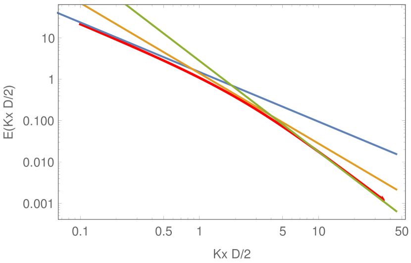
Figure 1: Thick red curve: $E(k_{x}D/2)$ in arbitrary units as function of $k_{x}D/2$. blue line : slope of -1.2. green line: slope of -2.2. yellow line : slope of -1.7.

4 numerical Results

The power spectrum $E(k_{x}D/2)$ for $m=1.2$, obtained by the numerical solution of equation (8), is displayed in Fig. 1.

It is seen that for $k_{x}D/2<<1$ the power spectrum has a logarithmic slope of $-1.2$ while for $k_{x}D/2>>1$ the logarithmic slope is $-2.2$, as expected from the analytical analysis presented above.

A line with a logarithmic slope of $-1.7$, the mean of the former two, which is tangent to the curve defines the "point of transition". One should note that the transition is a smooth one, and not a sharp break at a point.

From Fig. 1 it follows that the transition wavenumber, $k_{t}$, satisfies

$$k_{t}D/2=2.25\pm 0.05$$ (11)

So a given observational value of $k_{t}$ determines $D$. Expressing $k_{t}$by $x_{t}=2\pi/k_{t}$ , the observational transition spatial scale, leads to

$$D=(2.25\pm 0.05)\frac{x_{t}}{\pi}$$ (12)

Abramenko & Yurchyshyn (2020)found $x_{t}=0.85\pm 0.05$ Mm. Thus,

$$D=(0.57\pm 0.05){\rm\ Mm}$$

5 Concluding Remarks

The paper by Abramenko & Yurchyshyn (2020)provided a very neat power spectrum of the photosphere magnetic field of the quiet Sun. The high spatial resolution of the NIRIS data enabled a power spectrum down to spatial scales as small as $0.3$ Mm. This power spectrum exhibits what appears as two inertial ranges with logarithmic slopes of $-1.2$ and $-2.2$, for a spatial scale larger/smaller than $(0.85\pm 0.05)$ Mm, respectively.

The logarithmic slope of -1.2 corresponds to a 3- dimensional power spectrum with a logarithmic slope of -3.2. This is significantly shallower that the -3.67 value corresponding to Kolmogorov turbulence. The very interesting issue of the origin of such a power spectrum was not addressed here.

The present paper demonstrates that two inertial ranges actually correspond to a turbulence with a single inertial range with logarithmic slope equaling -1.2. The two ranges are manifestation of the fact that the observed infra-red emission is an integral along the line of sight. Since the value of $D$ is within the span of the lateral spatial scales probed, the transition shows up.

Interestingly, the value of the derived effective width is comparable to the width of the photosphere itself. This value of $D$ implied by the NIRIS power spectrum of Abramenko & Yurchyshyn (2020) is an observational constraint to be faced with theoretical models of near IR lines in the quiet solar photosphere.

In this context, a numerical model by Rueedi et al. (1998) yielded that the FeI15648 Å line is formed in the lower part of the photosphere and extends over a vertical span of about $0.1$ Mm. Their work refers to a sun spot and not to the quiet sun, and also assumes an absence of macro velocity turbulence. The situation here is different.

data availability

The article presents a theoretical research. It does apply the observational results of Abramenko & Yurchyshyn (2020) to the derived theoretical results.